chromgate v3.3.2 short guide - knauer - science …€¦ · the structure of the short guide is in...

ChromGate® V3.3.2

Short Guide

V7060-8 09/2012

Contents General Information............................................................................................................. 5

How to use this short guide ............................................................................................ 5

What ChromGate® is ...................................................................................................... 5

Supported Instruments ................................................................................................... 5

Installation of ChromGate® Software .................................................................................. 8

Administration ...................................................................................................................... 8

The Enterprise ................................................................................................................ 8

Creating and Configuring an Instrument ............................................................................. 8

Configuration – device communication port ................................................................... 8

Configuring the Interface ................................................................................................ 8

Configuring an Instrument .............................................................................................. 9

Auto Configuration ....................................................................................................... 10

Configuring Pumps ....................................................................................................... 10

Configuring Detectors .................................................................................................. 11

Configuring Assistant ASM 2.1L .................................................................................. 13

Configuring Autosamplers ............................................................................................ 14

Configuring Column Ovens .......................................................................................... 15

Configuring Switching Valves ...................................................................................... 15

Configuring a Manager 5000/5050 / IF2 ...................................................................... 15

Configuring a Flowmeter .............................................................................................. 15

Configuring a Fraction Collector .................................................................................. 15

Options – additional license options ............................................................................ 16

Generic Drivers ............................................................................................................ 16

Instrument Setup ............................................................................................................... 16

Instrument Setup of Pumps.......................................................................................... 17

Instrument Setup of Detectors ..................................................................................... 18

Instrument Setup of Assistant ASM 2.1L ..................................................................... 19

Instrument Setup of Autosamplers ............................................................................... 20

Instrument Setup of Switching Valves ......................................................................... 20

Instrument Setup of Column Ovens ............................................................................. 21

Instrument Setup of Flowmeters .................................................................................... 21

Instrument Setup of Aux Traces .................................................................................. 21

Instrument Setup of a Trigger ........................................................................................ 21

Instrument Setup of a Manager 5000/5050 / IF2 I/O ....................................................... 21

Instrument Setup of a Fraction Collector ..................................................................... 21

Instrument Setup Finishing ..................................................................................... 22

Instrument Status .............................................................................................................. 22

System Status .............................................................................................................. 22

Direct Control in Instrument Status .............................................................................. 22

Instrument Status of Pumps ......................................................................................... 23

Instrument Status of Detectors ..................................................................................... 24

Instrument Status of Assistant ASM 2.1L ..................................................................... 24

Instrument Status of Autosamplers ............................................................................... 25

Instrument Status of Column Ovens ............................................................................. 25

Instrument Status of Switching Valves ......................................................................... 25

Instrument Status of a Managers 5000/5050 / IF2 I/O ................................................. 25

Instrument Status of Flowmeters .................................................................................. 25

Instrument Status of Fraction Collectors....................................................................... 25

Knauer Instrument Control Method Option ........................................................................ 26

Conditioning the HPLC System ......................................................................................... 28

Direct Control ................................................................................................................ 28

Download Tab / Method ................................................................................................ 28

Starting a Preview .............................................................................................................. 28

Starting Single Runs .......................................................................................................... 28

Creating and starting a sequence ...................................................................................... 29

Sequence Table ............................................................................................................ 30

Chromatogram Evaluation ................................................................................................. 31

Loading Chromatograms .............................................................................................. 31

Working in the Chromatogram Window ........................................................................ 31

Changing the Integration parameters ........................................................................... 32

Calibration ..................................................................................................................... 33

PDA-Option ........................................................................................................................ 35

Performance Qualification .................................................................................................. 35

FRC Option (Fraction Collection) ....................................................................................... 35

FRC Installation ............................................................................................................ 36

Configuring Fraction Collectors .................................................................................... 36

Configuring a Virtual Fraction Collector ................................................................... 37

Instrument Setup with a Fraction Collector ................................................................... 38

Setup Fraction Collectors ............................................................................................. 38

Chromatogram Window ................................................................................................ 40

Instrument Status Fraction Collectors ........................................................................... 41

Displaying Fractions in the Instrument Setup during a Run ......................................... 42

Stacked Injection ........................................................................................................... 42

Evaluating Chromatograms ............................................................................................... 43

General Information 5

General Information

How to use this short guide

The user with basic chromatographic knowledge shall be enabled by help of this ChromGate

® Software short guide quickly to run a system. For an

example system (consisting of Smartline Pump 1000, Smartline Manager 5000, Smartline UV Detector 2600, Smartline Autosampler 3950 and a Smartline Valve Drive) the steps configuration, method creation, running an analysis, result evaluation and report are described. The basic control principles of all other supported instruments correspond to the described ones.

The structure of the short guide is in accordance with the main instrument control manual. Thus it becomes easy to find the there the detail descriptions as far as necessary.

What ChromGate® is

ChromGate® is a software package to control KNAUER HPLC

instruments as well as some other manufacturers including data acquisition and evaluation. Software licenses are necessary for unlimited use of ChromGate

®. Without license ChromGate

® starts in a demo mode.

This mode only allows the visualization and handling of demo data. Instruments cannot be controlled.

ChromGate® version 3.3.2 runs on computers with Windows XP

Professional (service pack 2 or higher) and Windows Vista Business or Ultimate, 32bit.The TCP/IP protocol and Microsoft framework .Net version 3 has to be installed.

For each HPLC system to be controlled one license is required. Different licenses for stand alone and for client server systems are available. For additional options like the 3D view of diode array detector (PDA) scans, the fraction collection (FRC), SEC, GPC, or the system suitability separate licenses must be ordered.

Supported Instruments

Following instruments are supported:

Pumps

AZURA Pump P 2.1L

AZURA Pumps P 2.1S / P 4.1S

Smartline Pump 1000 and 1050

Preparative Pump 1800 / WellChrom MacroStar K-1800

Smartline Pump 100 (RS-232 / LAN)

WellChrom MaxiStar K-1001 (LC 425, firmware 5.0 or higher)

WellChrom MaxiStar K-1000 (also K-1001 LC 410, firmware version below 5.0, a pressure trace cannot be acquired)

WellChrom K-501 (firmware version 1.23 and higher)

WellChrom MicroStar K-120

Kontron Pumps 320/322/325, 420/422/425, 520/522/525

Detectors

AZURA UV Detector UVD 2.1L

AZURA UV Detector UVD 2.1S

Smartline RI Detector 2300 / 2400

Smartline UV Detector 2500

Smartline UV Detector 2520 (RS-232 / LAN; limited data rate RS-232;

6 General Information

Smartline UV Detector 2550 (RS-232 / LAN; limited data rate RS-232; PDA option only for spectra required)

Smartline UV Detector 2600 (SCAN option for spectra required)

Smartline PDA Detector 2800 and 2850 (PDA option for spectra required)

Smartline UV Detector 200

WellChrom Mini-Detectors K-200, K-2000, K-2001, K-2300, K-2301, K-2400, K-2401, K-2500, K-2501

WellChrom Fast Scanning Spectral Photometer K-2600 (SCAN option for spectra required)

WellChrom Diode Array Detector K-2700 and K-2800 (PDA option for spectra required)

Shimadzu fluorescence detector RF-10 AxL (only 0.5 Hz data rate via RS-232, for higher data rates the 1 V integrator output with a KNAUER interface must be used)

Shimadzu fluorescence detector RF-20A/ AxL (FW version 0.9 only – must be installed from Knauer; 5 Hz data rate via RS-232, for higher data rates the 1 V integrator output with a KNAUER interface must be used)

Alltech conductivity detector model 650

Kontron Detectors 430/430A/432/435, 530/532/535

Kontron Diode Array Detector 540 (PDA option for spectra required)

Virtual detector

Since Kontron detectors do not have a digital data output, only detector control takes place over RS-232. Data acquisition is possible only with Kontron interface of KNAUER interface box.

Assistant

AZURA Assistant ASM 2.1L

Interface Modules

Smartline Manager 5000 / 5050 Interface Module

KNAUER Interface-Box IF2

KNAUER Interface-Box Model 96 (only integration version only recording and auto zero for the detector)

Kontron Interface Card

Autosamplers

Smartline autosamplers 3800, 3900, Knauer Optimas, 3950 (3950: RS-232 / LAN; LAN and 84+3 vials tray support firmware dependent)

WellChrom autosampler K-3800

Spark Autosamplers Marathon, Midas, Alias, Triathlon, Endurance

Kontron Autosamplers 360, 46X, 56X

Column Ovens

Smartline Column Oven 4050 (RS-232 / LAN)

JetStream Column Oven (from firmware b1.17)

Flow Meter

KNAUER Flowmeter

GJC Flowmeter

Bronkhorst Flowmeter

Electrical Valve Drives

AZURA valve V 2.1S

Electrical Valve Drives Smartline S 6, S 12 and S 16

Electrical Valve Drives WellChrom K-6, K-12 and K-16

Valco/VICI Switching Valves

General Information 7

Fraction Collectors (FRC-Option necessary)

KNAUER Smartline FC 3050

ISCO Foxy R1 / R2

ISCO Foxy Jr.

KNAUER MultiValve FC

Valco MultiValve FC

Buechi C660

Buechi C684

Vario 2000

Vario 4000

Virtual Fraction Collector

The ISCO Foxy 200 FC is discontinued due to different, not compatible firmware versions.

For details and possible control limitations refer to the instrument control manual.

For devices that supports RS-232 ASCII communicationKnauer can make a driver for basically functionality in ChromGate

® software via

Generic Drivers. Please ask for the conditions.

8 Creating and Configuring an Instrument

Installation of ChromGate® Software See Installation Guide / Instrument Control Manual

Administration

See administration manual

The Enterprise

Inside the Enterprise a directory structure like that of the windows level can be created. A Location/Group can be created and stored like a folder. At each hirarchy level you can create Instruments.

An Instrument is the description of a HPLC system. In these Instruments all single devices of the HPLC system are involved, which shall be controlled or used for date acquisition. Such an Instrument is later on the base for creation of methods.

The structure items „Location/Group“ and „Instrument“ are visible in the „Enterprise“ only. They will not be displayed within the Windows Explorer.

To create a new Instrument click in the ChromGate® start window on File – New – Instrument. New Folders can be created with the menu sequence File – New – Location/Group.

Creating and Configuring an Instrument Configuring the system involves the selection of the instruments and features that are to be used (during installation, each component of the HPLC system is registered on the network). Once an instrument configuration has been made it can be easily retrieved.

Any detector or sensor producing an analog signal which can be digitized with an A/D card or Interface Box can be used for data acquisition. You must configure your data acquisition interface before you can acquire analog data using the data system.

For more detailed information, please refer to the Instrument Control Manual.

Configuration – device communication port

Some of the devices have two communication ports on the rear panel for controlling the device by the computer. One is an RS-232 port, also called serial or COM port; the other is an Ethernet port, also called LAN (Local Area Network). Beside the Knauer valve drives, for all the devices the desired communication port must be defined in the device. Please pay attention to the corresponding notes in this manual and refer to the device’s manual for more information, how the desired communication port must be configured. Please note, that for some devices the functionality depends on the selected communication port.

Configuring the Interface

Click the Tools/Interface Configuration command from the ChromGate Main Menu. A window will appear displaying several possible interface devices. To configure a device, click on the icon to select it then click the Properties button or double click on the instrument icon (Fig. 1).

Creating and Configuring an Instrument 9

Fig. 1 Dialog box for configuring the Manager 5000

If you configure the interface newly the message like Fig. 2 will remind you to enter the serial number of the interface device.

Fig. 2 Error message for missing serial number

Configuring an Instrument

After creating a new Instrument (see page 8) it must be configured. The icon of any not configured Instrument is characterized by a question mark.

Right click on that instrument icon and than select Configure – Instrument. Click on the Configure button in the opened window without having changed the Instrument type „KNAUER HPLC System“.

Fig. 3 Instrument selection window

Several icons will be displayed in the Available Modules box on the left. Add modules to be configured by double-clicking on each, or by clicking

once on the icon, followed by the green arrow .

Now configure each module (detector, pump, autosampler, or event configuration) separately. If you try to exit the window with OK and one or more instruments are still not configured, an error message will appear.


It is recommended to configure any selected module before selecting the next one.

Not configured instruments are indicated by a question mark on the corresponding icons.

Auto Configuration

Using the <Auto Configuration> -button, all devices, connected via LAN and switched on, will be automatically added and configured in the instrument.

Fig. 4 Auto Configuration start window

All Knauer devices use a single IP port for LAN communication. Only devices with the same IP port as selected in the Auto Configuration window will be found. The default IP address is 10001. It can be changed manually in the device’s setup.

We recommend reviewing the configuration of all automatically added devices. Devices connected via RS-232 (serial connection) will not be found and must be added manually.

Configuring Pumps

For each pump to be configured double-click the icon in the Configured Modules window and complete the configuration dialog.

Fig. 5 Pump S 1000 configuration window

Please note


1. If a device is controlled vial LAN, from the connected device the

configuration can be read-out by software by using the -button (recommended). In this case the following steps must not be done manually, but it is reqcommended to review the read-out configuration.

2. Use a name which is unique within the instrument.

3. The selected Gradient Mode must correspond to the setting directly at the pump (see pump manual).

4. Select from the drop-down list Interface or Serial Port the serial port or network number for the communication port on your PC where the pump is connected.

5. Entering the Serial Number is necessary for pumps running via KNAUER network and all pumps running via LAN, if the option “Identify device by serial number” is enabled (recommended setting).

6. The selected Head must correspond to the setting directly at the pump (see pump manual).

7. Select from the Pressure units drop list the desired unit.

When complete, click OK to exit the dialog and to save the settings.

Configuring Detectors

For each detector to be configured double-click the icon in the Configured Modules window and complete the configuration dialog.

Fig. 6 UV Detector 2600 configuration window


Please note


configuration can be read-out by software by using the -button (recommended). In this case the following steps must not be done manually, but it is recommended to review the read-out configuration.


3. Select from the drop-down list Interface or Serial Port the serial port or network number for the communication port on your PC where the detector is connected.

4. Enter the Serial Number.

5. Select the number of used channels.

If a non-supported detector will be used, the 1V integrator output of this detector must be connected with the Analog In of the Interface Box (KNAUER Interface Box IF2, Manager 5000 interface module, KNAUER HPLC Interface Box. In the configuration dialog the User Defined Detector must be selected.

Fig. 7 User Defined Detector configuration window

Select the already configured interface in the Interface drop-down menu.

Click then on the button to open the channel configuration. Select the interface and the channel you want to use.

Fig. 8 User Defined Detector channel configuration window



Configuring Assistant ASM 2.1L

The Azura assistant ASM2.1L is a modular instrument, that allows to combine up to 3 devices. The follwing devices can be included:

- pumps P2.1S, P4.1S

- detector UVD2.1S

- Knauer valve drives with 2, 6, 12 and 16 positions

- Valco valve drives with 2, 6, 8, 10, 12 and 16 positions

Configuration rules:

- Two pumps are only supported as HPG, both pumps must have the same pump head, three pumps are not supported.

- Only one UV detector is allowed.

- One valve drive can be used as a fraction collector, if the Knauer Fraction Collector Control option is installed and the appropriate license option is used. Cascading fraction valves is not supported. This is also applicable, if the valves are installed in different ASM2.1L housings.

- All the devices will be controlled by only one LAN port, a serial control via RS-232 is not implemented.

- Pumps cannot run in a HPG, if they are installed in different ASM2.1L housings.

Fig. 9 Assistant ASM2.1L configuration window, tab General

The Assistant ASM2.1L supports LAN connection, only one LAN port for all 3 devices is required. The configuration window has four tabs, one for general settings and one for each of the three device positions, left, middle and right. While the General tab allows for settings for the whole assistant, the device tabs give the option to configure the included devices.

Please note

1. If the ASM has been added by Auto Configuration or the modules

have been read-out by using the -button (recommended), the following steps must not be done manually, but it is recommended to review the read-out configuration.


2. For the Assisitant as well as for the single modules use a name which is unique within the instrument.

3. If two pumps are configured, select “HPG A” and “HPG B” for the pumps.

4. Enter the Serial Number of the Assistant.

5. The selected Head (pumps only) must correspond to the setting directly at the pump (see pump manual).

6. Select from the Pressure units drop down list the desired unit (pumps only).

7. If a valve is selected as fractionation valve, the complete setup for a MultiVavle FC will become available. Please note, that a a fraction valve from the Assistant can not be cascade with other valves to expand the number of available fraction ports.


Configuring Autosamplers

For the autosampler to be configured double-click the icon in the Configured Modules window and complete the configuration dialog.

Fig. 10 Smartline Autosampler 3950 configuration window

Please note

1. If a S 3950 is controlled vial LAN, from the connected device the serial number (recommended). All other configuration settings must be done manually.


3. Entering the five digit Serial Number is optional for autosamplers.

4. The Device ID must correspond to the setting directly at the autosampler (see autosampler manual).

5. Select from the drop-down list Serial Port the serial port or network number for the communication port on your PC where the autosampler is connected.

6. The Tray configuration must correspond to the setting directly at the autosampler (see autosampler manual).


7. If you are using the oven and/or the tray cooling the Column oven and/or Tray cooling must be activated in the Options area.

8. If you are using a high capacity syringe the Prep mode must be activated.


Configuring Column Ovens

See Instrument Control Manual

Configuring Switching Valves

The switching valves icon refers to a group of the switching valves; each of them must be configured before using in an instrument method. Double-click the icon and complete the configuration dialog.

Fig. 11 Configuration window for the switching valves

Please note:


configuration can be read-out by software by using the -button (recommended). In this case the following steps must not be done manually, but it is recommended to review the read-out configuration.

2. Each valve must be selected and configured separately Fig. 11.


4. Each valve is connected to a separate Serial Port.


Configuring a Manager 5000/5050 / IF2

A Manager 5050 must be configured as a Manager 5000.


Configuring a Flowmeter


Configuring a Fraction Collector

See chapter FRC Option (Fraction Collection) on page 36

16 Instrument Setup

Options – additional license options

The use of additional optional licenses requires activating the corresponding options. Click in the Instrument selection window Fig. 3 on the Options button and activate the desired options. Please note, that ChromGate will check while opening an instrument, if the enabled license options are available. If not, the instrument will not open.

Generic Drivers

KNAUER develops on demand Generic Drivers for devices supporting RS-232 ASCII communication. For the programming we need the instrument manual and its communication protocol. Please ask you distributor for the conditions.

Instrument Setup After configuring a new Instrument open the Instrument Setup with a double click on instrument icon or make a right mouse click on the icon and select Open from the menu.

Fig. 12 ChromGate® start window

Alternatively you can right click on the instrument icon and than decide to open the Instrument Setup in online or offline mode.

Opening the method window starts automatically a wizard. Its use may be helpful but not all possible software functions are accessible within.

To program the method parameters in the Instrument Setup select

Method – Instrument Setup or click on .

The Instrument Setup includes method and device parameters which are executed during a Single Run) or a Sequence. Any configured module is shown on an own tab. The appearance depends as well on the module type as on its configuration.

In the lower part a graphic is displayed, unique for the whole HPLC system and showing the flow rates, gradients, wavelengths and possible other profiles (Fig. 13). For details refer to the ChromGate

® Reference

Manual.

Instrument Setup 17

Fig. 13 Instrument setup window (Smartline Pump 1000)

Instrument Setup of Pumps

In the Instrument Setup (Fig. 13) all parameters of the pump can be programmed.

Please note

1. The Working Mode cannot be changed here. It is part of the Configuration.

2. The Pump Program is a table, in which time, flow rate gradient composition, and signal outputs can be entered. The appearance of the table depends on the pump configuration.

3. Rows with identical time setting are not allowed. The minimum time difference between two lines is 0.02 minutes.

4. In the HPG-Modus all gradient changes are transferred automatically to the involved pumps. This is not valid for digital Events.

Fig. 14 Gradient table

5. The Pretreatment times must be entered as negative values, because they are relative to the zero injection time.

If a pretreatment is to define for more than one instrument (pump and/or valve drive) in a method, it is recommended to set for all of them the earliest time. All pretreatment procedures will start simultaneously.

18 Instrument Setup

Instrument Setup of Detectors

In the Instrument Setup all parameters of the detector can be programmed.

Fig. 15 Smartline UV Detector 2600 Instrument setup window

Please note

1. You must have activated as many channels in the detectors Configuration, as you want to use for data acquisition.

2. For calibrations and subsequent measurements the Time constant and the Sampling rate the same settings must be done.

3. The Wavelength Program (Fig. 16) is a table, in which time and the wavelengths for each channel can be entered. The appearance of the table depends on the detector configuration.


5. Do not change the Bandwidth setting. This would lead in future measurements with the method to deviating peak areas at same concentrations.

Fig. 16 Smartline UV Detector 2600 time table

Instrument Setup 19

Instrument Setup of Assistant ASM 2.1L

Due to the modular system, there are a lot of possible configurations for the ASM2.1L. The setup window will look different, depending on the configured modules. The settings for pumps, detector and valves correspond to the setup of the single devices.

Fig. 17 ASM 2.1L setup window for pump, valve, detector

Please note

1. The ASM has always an own run time.

2. The Time Program includes an own line for all modules + for the ASM to program the Events (Digital Outputs). If a new line must be added, it is only required to add the line for the module you want to change the setting.

3. If an HPG was configured, you can only program pump A directly.

4. Rows with identical time setting for the same module are not allowed. The minimum time difference between two lines is 0.02 minutes.

20 Instrument Setup

Instrument Setup of Autosamplers

In any system you can include only one autosampler. The control parameters for the autosampler become part of your method and sequence files.

Fig. 18 Smartline Autosampler 3950 setup window

Please note

1. In case of Full loop injections the loop will be flushed to ensure removing the previous sample completely.

2. Enter the Flush volume. In case of Full loop injections the volume is fixed at 30 µl.

3. The accuracy and reproducibility of the autosampler may decrease if headspace pressure is switched off.

4. If you are using the oven and/or the tray cooling the Column oven and/or Tray cooling must be activated in the Configuration.

5. Use Timed events to program Events which will be executed during a run at the set times.

6. With Mix methods you can program pretreatment methods to be executed prior the injection.

7. The Stacked Injections mainly is interesting for preparative applications. Please refer the FRC chapter of the instrument control manual.

Instrument Setup of Switching Valves

The setup procedure for injection valves and switching valves is identically. The valve type was selected within the configuration. In the Instrument Setup the switching times are programmed in a time table.

Instrument Setup 21

Fig. 19 Instrument Setup valves

Please note


2. The Pretreatment times must be entered as negative values, because they are relative to the zero injection time.

3. If a pretreatment is to define for more than one instrument (pump and/or valve drive) in a method, it is recommended to set for all of them the earliest time. All pretreatment procedures will start simultaneously.

Instrument Setup of Column Ovens


Instrument Setup of Flowmeters


Instrument Setup of Aux Traces


Instrument Setup of a Trigger

Any configured HPLC system with at least one detector acquisition channel will be completed by an additional tab for the trigger.

Click on the Trigger tab to designate the trigger type and to setup the synchronization. The trigger type determines how the data sampling and the gradient program(s) are started.

The default set trigger type External (Extern) is the most used one. If this option is selected no further settings are necessary.

Instrument Setup of a Manager 5000/5050 / IF2 I/O


Instrument Setup of a Fraction Collector

See FRC option, chapter Setup Fraction Collectors on page 38

22 Instrument Status

Instrument Setup Finishing

When all settings for all components are done save the method with File

– Method – Save, Save As or - Save Method.

Instrument Status Within the Instrument Status you will find to different types of status information, the System Status and the Instrument Status.

System Status

All configured devices are displayed together on one tab. During a run all actual parameters like flow rate, pressure, signal levels, switching positions, temperature will be red out and displayed. If no transferred data are available the parameter will be indicated by n/a.

Fig. 20 Instrument Status window, system status

Direct Control in Instrument Status

The single instrument tabs of this window provide more detailed information. They also enable Direct Control of the system. On these tabs you have the possibility of directly controlling the individual instruments. This is even possible while a method is running.

The active state of the communication with an instrument, necessary for

controlling it, is represented by the green LED symbol. The grey LED

symbol ( ) represents an inactive status.

Fig. 21 Instrument status tab, example: Smartline Pump 1000

To create a new method, open the Instrument Status by clicking on Control - Instrument Status. With any opening of the status window default values will appear which not correspond to the actual instrument parameters, for instance in case of a pump a flow rate of 1 ml/min.

The Direct Control enables as well to control the included instruments without starting the method as to change the programmed time table during a run. For this case the option Direct Control during a run inside the Runtime Settings (see page 26) must be activated. Select Method - Runtime Settings and activate the option field Enabled. Now you can decide with Save changes in time table if the changes shall be stored or not.

Activating „Direct Control“ is a global feature. It becomes valid for all runs with all methods until it will be deactivated again.

Instrument Status 23

Instrument Status of Pumps

For any pump the parameters set in the Configuration will be red out and displayed (Fig. 22).

Fig. 22 Instrument status tab, example: Smartline Pump 1000, LPG mode

The Monitor area displays the permanently actualized instrument and time table parameters.

The Direct Control area enables to change the flow rate (Flow Apply), the gradient composition (Gradient Apply), the pressure limits (Control Pressure limits) and the Digital Outs.

The option „Gradient Modify“ is accessible only during a run and exclusively for KNAUER pumps.

Fig. 23 Gradient modify window

The gradient spread sheet is a copy of that out of the Instrument Setup window. Here the elapsed lines are grayed. The red line shows the actual gradient status. The yellow ones are that which are open for modifying.

To change the gradient program, the desired values must be entered in the fields on the top of the window. A click on Commit Line inserts it into the gradient program. The change by one or more committed lines becomes active by a click on Send Gradient.

Please consider that the data acquisition time must be adjusted to the changes via „Control – Extend Run“ to ensure a complete chromatogram. For instance freezing the gradient for 3 minutes requires a prolonged run time by 3 min.

24 Instrument Status

Instrument Status of Detectors

For any detector the parameters set in the Configuration will be red out and displayed (Fig. 24).

Fig. 24 Instrument Status des Smartline UV Detectors 2600

The Monitor area displays the Run Status and for each detector channel, the output values and as far as available the wavelength.

The Direct Control area enables to switch the Lamp on/off, to perform an Autozero, to change the wavelength for the desired channel (Ch.#) via WL Apply and the Digital Outs via DO Apply.

Click this button to use the diagnostic features of the ChromGate®

software. The Diagnostics window appears which allows you to access information and to control important parameters and modules of the device.

Instrument Status of Assistant ASM 2.1L

The Assistant status window allows for checking the current status of all configured modules of the Assistant and the direct control.

The status and direct control options in this window depend on the configured modules. The options in the majority directly match with the options for the single devices.

Fig. 25 ASM2.1L status tab – valve, valve, pump

If an HPG is configured, the Flow and A(%) for the gradient can be enabled separatly. The <Apply> -button will send the values for the enabled option(s), either only Flow or A(%) or both.

Instrument Status 25

Instrument Status of Autosamplers

Fig. 26 Smartline Autosampler 3950 status tab

Again there are the areas Monitor to display the status parameters and Direct Control enabling to change/set the Oven Temperature, the Tray Temperature or to start a Needle Wash.

Instrument Status of Column Ovens


Instrument Status of Switching Valves

The Instrument Status displays for any valve the actual position, which can be changed via the drop down list and subsequent verifying with Set Position.

Fig. 27 Status tab, switching valves

Instrument Status of a Managers 5000/5050 / IF2 I/O


Instrument Status of Flowmeters


Instrument Status of Fraction Collectors

See FRC option, chapter Instrument Status Fraction Collectors on page 41.

26 Knauer Instrument Control Method Option

Knauer Instrument Control Method Option You can generally activate options, valid for all runs of all methods.

Fig 28 Instrument Setup Method menu

Runtime Settings

Fig 29 Knauer Instrument Control Method Option - Runtime Settings

Via Method – Runtime Settings (Fig 29) you can enable the change of methods in Direct Control during a run and to Save changes in time table. You also can define the handling of error situations (see Instrument Control Manual).

Clicking on the Advanced button will open the advanced runtime settings setup.

Knauer Instrument Control Method Option 27

Fig 30 Knauer Instrument Control Method Option - Advanced Runtime Settings

The Check run time when saving method option will check the programmed run times of all devices an gives a warning message if there are different.

Power all device up at: allows to switch on the detector lamps and will wake-up the AZURA, PLATINblue and newer Smartline devices (S 1050, S 2550, S 2520) from Standby. The Standby wake-up will not work for older Smartline devices as pump S 1000 or detector S 2600.

Trace name will add the wave length of the first line in the wave length table of all those detectors as a channel name for the detector trace. It will be shown in the chromatogram and also later on in the run report, but not in the channel selector.

Activated options in this window become valid for all instruments in the Enterprise.

Solvent Control

Via Method – Configure Solvent) you can configure the control of the eluent reservoirs (See Instrument Control Manual).

Custom Report

ChromGate®

provides standard reports for Area %, Baseline Check, System Check, Fraction Report, External Standard, Internal Standard and Normalization which can be printed out. With the option Custom Report you can multiple own reports.

Clicking on Method – Custom Report) will open the Custom Report editor to create the different designed reports (See Instrument Control Manual).

Advanced

Export, Custom Parameters, Column/Performance, Files, Advanced Report (See Instrument Control Manual).

Validation of Integration


Properties

Click on Method – Properties to select the desired method options or functions like the kind of calibration, the time of validation, or activation the Audit Trail. Details you will find in the Reference Manual.

28 Starting Single Runs

Conditioning the HPLC System You can start conditioning the HPLC system on different ways:

Direct Control

The direct control during a run option is a valuable tool for method development but can also lead to the possibility for unintended changes to the method. For this reason, it is recommended that this option not be enabled, especially for routine methods. For more information see chapter „Direct Control in Instrument Status“ on page 22.

Download Tab / Method

The actually set parameters (may be even not saved) of the current instrument setup tab as well as those of the whole method can be downloaded to the corresponding instruments. Select the menu

CONTROL – DOWNLOAD METHOD or

CONTROL – DOWNLOAD TAB

In case of Download Tab, only a single pump will be controlled even for an HPG system.

Starting a Preview

To collect data during the equilibration a Preview must be started by

clicking on Control – Preview or . The Preview starts immediately without injection even if a trigger is defined. The program remains in the first line. The preview must be stopped manually (maximum time 400 minutes). To start a Single Run the Preview must be stopped before.

Starting Single Runs After equilibration you can start a single via Control – Single Run or by

clicking on . The following dialog will appear.

Fig. 31 Single run start window

Enter the necessary items (See Reference Manual) and click on the Start button.

Creating and starting a sequence 29

Stopping a run

Each run can be stopped at any time by a click on the button. Confirm the run stop in the opened window.

Fig. 32 Run stop window

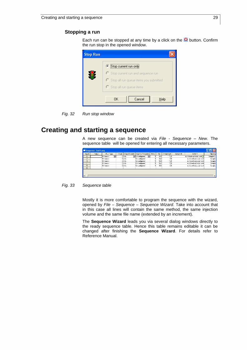
Creating and starting a sequence A new sequence can be created via File - Sequence – New. The sequence table will be opened for entering all necessary parameters.

Fig. 33 Sequence table

Mostly it is more comfortable to program the sequence with the wizard, opened by File – Sequence – Sequence Wizard. Take into account that in this case all lines will contain the same method, the same injection volume and the same file name (extended by an increment).

The Sequence Wizard leads you via several dialog windows directly to the ready sequence table. Hence this table remains editable it can be changed after finishing the Sequence Wizard. For details refer to Reference Manual.

30 Creating and starting a sequence

Sequence Table

Due to its length the sequence table as shown in Fig. 34 is split in three parts.

Fig. 34 Sequence table

After saving the sequence table the sequence can be started with a click

on or via Control - Sequence Run. Both will open the following window:

Fig. 35 Sequence start window

Enter the necessary items (See Reference Manual) and click on the Start button.

The run ort he sequence can be interrupted by clicking on the button. In the opened window (Fig. 32) the choice of interruption must be confirmed. For details refer to Reference Manual.

Submit

During any Single Run or running sequence you can enter details regarding the next runs. By a click on Submit it will be arranged in the queue and started when all previous runs are finished. For details again refer to Reference Manual.

Chromatogram Evaluation 31

Chromatogram Evaluation

Loading Chromatograms

To evaluate or to change a chromatogram it must be loaded. Click on

or select File – Data – Open, highlight the desired chromatogram and click on Open. Alternatively you can double click on the selected chromatogram.

Fig. 36 Chromatogram selection window

All saved chromatograms are stored with the method used for acquiring it. However, you can open chromatograms also with other methods, which will be defined via Options. Details you will find in the Reference Manual.

Working in the Chromatogram Window

After loading it the chromatogram can be treated in numerous ways. The possibilities will here only be listed to give an overview. Details are to be red in the Reference Manual.

Add Trace

Add Multiple Trace

Axis Setup Graph title

X-/Y-Axis Use this range General Options

Annotations

Appearance

Full Unzoom

Clear Overlays

Operations

Click on Operations, to select one of the following possibilities:

Move Trace Stack Traces

32 Chromatogram Evaluation

Align/Stretch/Normalize Smooth/1

st Derivative/

2nd

Derivative Add/Subtract/Multiply/Divide

Properties

Click on Properties, to select one of the following possibilities:

Trace Setup Annotations Hide Details Reset Scaling Axis Setup/Appearance

Graphical Programming

All parameters for chromatogram treatments are listed under Graphical Programming. They are also available as icons at the bottom of the chromatogram window.

Utilities

You have the choice to Print the loaded chromatogram or to Copy to Clipboard from where you can insert it for instance into a word file. The (treated) chromatogram can be stored with Save Trace.

Changing the Integration parameters

Integration Events

Various parameters like Width, Threshold, Baseline and more have to be defined for the evaluation of analytical results. The Integration

Events table is opened via Method – Integration Events or a click on .

Fig. 37 Integration Event Table

For details refer to Reference Manual.

Manual Integrations Fixes

This table, opened via Method Manual Integration Fixes or a click on , is comparable to the Integration Events table. However all parameters will be applied only to the actual opened Chromatogram and stored with it. Thus individual chromatograms can be optimized without changing the general method. For details again refer to Reference Manual

Using the Icon bar

For recalculations of chromatograms you can use the icon bar at the bottom of the chromatogram window. These icons correspond to the parameters (Events), which you find in the tables Integration Events and Manual Integration Fixes.

Fig. 38 Icon bar for chromatogram modifications

Chromatogram Evaluation 33

Width 0.2 and Threshold 50 are set as default in the Integration Events table. The start and stop times are set to 0.

In any case values for „Width“ and „Threshold“ must be entered into the table. Otherwise no integration is possible.

The changes according to the new settings can be seen after

recalculating the chromatogram by clicking on Analyze Now or .

Width

Threshold

Extremely large as well as extremely small values for „Width“ and „Threshold“ may cause that some peaks will not be integrated.

Shoulder Sens

Int Off

Valley

Horiz BL horizontal base line

Bk Horiz BL horizontal base line from a value to the peak end

LP Horiz BL horizontal base line at the lowest point of chromatogram

Tan tangent

Front Tan tangent at the peak front

Min Area

Neg Peak

Disable Peak End

Reassign Peak

Man BL manual base line

Man Peak manual peak

Split Peak

Force PK Start

Force PK Stop

Move Baseline

Reset Baseline

Reset BL at Valley

Calibration

For quantitative evaluations of chromatograms the used method must involve a calibration. This will correlate the measured peak areas or heights with the concentrations of interested components.

The calibration is a part of the method. As well one point calibrations (always leading through the point of origin) as multiple point calibrations are possible. For these you can decide whether the path the point of origin or not.

Two different calibration techniques are possible. However, any method can involve only one of them:

Calibration with external Standards

For this method you have to take separate chromatograms of different known concentrations of the standard substance always using the same

34 Chromatogram Evaluation

injection volume. To obtain the calibration curve the measured peak areas or heights are plotted versus the concentrations.

Calibration with internal Standards

For this method a defined amount of a known substance (internal standard) will be added to the sample and to the standard prior to the sample preparation. This substance cannot be one of those to be determined. The calibration curve is obtained in the same way as for the external standard method. For evaluations than the measured peak areas or heights are related to the internal standard.

The advantage of the method consists in the independence of the results on injection volumes and possible substance lost during sample preparations.

Generally the calibration can be performed for single substances as well as for substance groups. For details refer to the reference manual with following topics:

Calibration Setup.

Calibration Theory

Single Level and Multiple Level Calibrations

Replicates and Averaging Calibrations.

Steps for Creating a Calibration

Creating Calibrations Graphically

Define Single Peak

Peak Table

Calibrating Your Method (Running Calibration Samples

Single Level Calibration Using a Stored Data File

Reviewing Calibration Curves

Groups and Group Calibration.

Defining a Group

Group Table Properties

Uncalibrated Range

Group Calibration (Calibrated Range)

Group Table

Group Range Definition

FRC Option (Fraction Collection) 35

PDA-Option With a PDA detector you can evaluate the runs and their chromatograms additionally by help of spectra. However, you need an additional PDA license.

The PDA Option has to be activated in the „Configuration“ of the detector. To do this the additional PDA license is required.

Details for running PDA detectors you find in the Instrument Control Manual. The chapter ChromGate

® PDA Option includes the sections:

Method PDA Options

Library

Purity

Spectrum

Multi-Chromatogram

Ratio

PDA View

Working with 3D Data

Creating a Spectral Library

Adding Spectra to a Library

Searching Spectra

Overlay Spectra

Add Multi-Chromatogram to Table

Performance Qualification Details for performing system tests you find in the Instrument Control Manual. The chapter Performance Qualification includes the sections:

Conditions

Settings

Measurement

Test Report of the Performance Qualification

FRC Option (Fraction Collection) The FRC Option provides the possibility to collect fractions via detector signals and to indicate them in the chromatograms. Any programming of the included fraction collector is not necessary. The collection can be time programmed or controlled via the signal level, the slope at the ascending and descending flange of the peak and/or the spectrum of the peak.

The fraction collection is programmed in a time table. For any peak of the chromatogram you can define the conditions separately. For instance the collection of a fraction may start with a set slope at the ascending flange of the peak and stop by signal level falling below a threshold. The peak purity obtained by comparing spectra also can be used as a collection condition. This of course requires the use of a PDA detector and therefore the additional PDA option is necessary.

The FRC Option also includes a virtual fraction collector. By help of this tool you can optimize the fractionation on the base of only one chromatogram. No further real analysis are necessary.

36 FRC Option (Fraction Collection)

Additional applications are the peak and the solvent recycling abilities. The solvent recycling is practically limited to isocratic eluent flows, whereas the peak recycling can be applied in any method to lead back the collected fraction to a second path through the column for better purification. Normally additional valves are required for this task. They are not necessary if a MultiValve collector is in use because two defined switching positions here can be used.

FRC Installation


Configuring Fraction Collectors

The configuration of fraction collectors is to perform together with other the instruments as it was described in the chapter Inside the Enterprise a directory structure like that of the windows level can be created. A Location/Group can be created and stored like a folder. At each hirarchy level you can create Instruments.

An Instrument is the description of a HPLC system. In these Instruments all single devices of the HPLC system are involved, which shall be controlled or used for date acquisition. Such an INSTRUMENT is later on the base for creation of methods.

The structure items „Location/Group“ and „Instrument“ are visible in the „Enterprise“ only. They will not be displayed within the Windows Explorer.

To create a new Instrument click in the ChromGate® start window on File – New – Instrument. New Folders can be created with the menu sequence File – New – Location/Group.

Creating and Configuring an Instrument on page 9. Any HPLC system can include only one fraction collector.

For the fraction collector to be configured double-click the icon in the Configured Modules window and complete the configuration dialog.

The configuration window appears similar for all fraction collectors, except the KNAUER MultiValve fraction collector.

Fig. 39 FC Foxy Jr. configuration window


Please note:


2. Entering the five digit Serial Number is optional for fraction collectors.

3. The Vial Volume (ml) will be set automatically according to the selected rack. You can overwrite it with smaller values. If the fraction volume exceeds the setting the collection is continued in the next free position.

4. With the setting of Tubing Parameters you take into account the time delay for transporting the sample from the flow cell to the collector valve.

Fig. 40 Tubing parameters setup

5. To configure the Solvent/Peak Recycling an additional valve has to be configured. In case of the MultiValve the second last and the last but two switching positions will be defined.

Fig. 41 Solvent/Peak recycling setup MultiValve FC

6. For the MultiValve collector each of the included valves must be selected and configured with a separate Serial Port.


Configuring a Virtual Fraction Collector

The virtual fraction collector is a tool to optimize the fractionation without need for sample and eluent or to collect fractions while simulating an already taken chromatogram. The configuration procedure is the same as for normal collectors.


Instrument Setup with a Fraction Collector

In any system you can include only one fraction collector. However, the setup window is independent on the configured fraction collector.

This window differs in one respect from other setup windows. It is not only important for setting up the fraction collector. It is also used during the runs showing the taken chromatogram indicating the collected fraction areas and those of solvent and peak recycling. This view remains until the next run will be started.

As the proceeding chromatogram is displayed you can collect fractions with the Direct Control facilities.

Setup Fraction Collectors

All parameters of the fraction collector can be programmed in the Instrument Setup window (Fig. 42).

Fig. 42 Fraction Collector Instrument Setup window

Please note:

1. Always signals of the selected Detection Channel are responsible for the collection.

2. Enter the pump’s flow rate to allow the software to calculate the volumetric delay. If you press the Update Flow button if the pump’s setup is already finished, the software will escape the flow from the pump’s setup.

3. The collecting conditions and retention times are programmed in the time table Fraction Collector Program.

4. The time of the first row is fixed to zero (start time).

In the column Mode the collection algorithms can be set separately for each time window:

− Single Event to define the conditions for begin and end of the fraction. Therefore always two conditions have to be defined by selecting them from the Event drop down list.


− Peak Recognition to define the conditions for begin and end of all fractions within the time window or the whole chromatogram.

The Events are always programmed in combination with the Parameters and the retention time (Exp. Interv. Time).

Following conditions are available in the Single Event mode:

− Unconditional − Signal Level − Signal Slope − Signal Level/Slope − Local Maximum − Local Minimum − Spectral Similarity as far a PDA detector is used

Following conditions are available in the Peak Recognition mode:

− Signal Level − Signal Slope − Signal Level/Slope − Spectral Similarity as far a PDA detector is used

Exp. Interv. Displayed according to the settings in the Parameters field

Rel. time shift it cannot be defined in the first row (start time zero)

When the collection conditions are set the corresponding Parameters values are to define.

Fig. 43 Defining the fractionation parameters for Single Event

Define the Signal Level (Units) for the Ascending and Descending flange of the peak and than select the Action (Fig. 43).

In the field Action the handling of each fraction is to define:

Collect To select Next for using the next free position or select position followed by entering the desired position number.

Waste

Solvent Recycling

Peak Recycling The fraction is led back via the pump to the column.

None solely a marker is set at the defined time Collect Slices the fraction is collected in constant volume steps in

several vials.

Proceed in the same way if begin and/or end of collection shall be defined by a Local Maximum or a Local Minimum.

For collection according Spectral Similarity first define the Ascending or Descending peak flange before you select the Ref. Spectrum.


With the activated Fraction Check option the run will stop if the defined collection conditions do not fit the peaks of the actual taken chromatogram.

At last the rack has to be configured or loaded.

Stacked Injection

The option Stacked Injection allows to perform injection during a run. As an injection device the autosampler 3950 or the Injection Module can be used. Please refer the Instrument Control manual for the configuration and setup.

Chromatogram Window

In the lower part of the Setup window a Chromatogram Window is shown. If already chromatograms were taken with the actual loaded method the last loaded one will be displayed. Of course you can load any other stored chromatogram to use it for programming the time table.

Fig. 44 Programming the time table

Fig. 45 Example for a time table

The option Pretreatment can be used to avoid different retention times caused by different injection volumes. The Solvent Recycling can be applied to that period.

For the stacked Injections option, please refer the instrument control manual.


Instrument Status Fraction Collectors

The Instrument Status of fraction collectors consists of two tabs, the Monitor / Direct Control and the Rack View.

Monitor / Direct Control

The status of a fraction collector includes two tabs, Monitor/Direct Control and Rack View. The Monitor area displays the permanently actualized instrument and time table parameters.

The Direct Control area enables to change before or during a run the positions of the fraction collector or to select the positions Waste, Solvent- or Peak Recycling.

To use the direct control option during a run, the option „Direct Control during a run“ inside the „Runtime Settings“ (see page 26) must be activated.

According to the settings in the “Runtime Settings”, the changes made to the settings and applied during a run will either be automatically stored in the method or rejected after the run. The corresponding new lines in the spreadsheets are marked with the comment DC Operation (Direct Control Operation).

Rack View

Fig. 46 Rack View example

The displayed rack corresponds to the configured one. All already used vials will appear green highlighted. Moving the cursor across the rack will change the upper descriptive line. There the vial number, the begin and end of collection and the collected volume is displayed (see the arrows in Fig. 46).

For MultiValve fraction collectors the rack may show more fraction positions as available for the configured valve(s). The driver will ignore the not existing positions.


Displaying Fractions in the Instrument Setup during a Run

Start a Single Run or a Sequence as usual (see page 28 through 30). During any run the chromatogram is displayed in the Instrument Setup of the fraction collector. Collected fraction areas are highlighted green, Peak Recycling areas red and Solvent Recycling areas blue.

Fig. 47 Fraction collector instrument setup window (after a run)

Stacked Injection

The option Stacked Injection allows to perform injection during a run. As an injection device the autosampler 3950 or the Injection Module can be used. The injection module consists of a pump and a Knauer 2-position switching valve. Optional an injection loop can be used. As a pump a pump P 2.1L, P 2.1S, P 4.1S, S 100, S 1050 or 1800 can be selected.

Fig. 48 Injection module configuration window

Evaluating Chromatograms 43

In the instrument setup for the S 3950 as well as for the injection module a button <Stacked Injections> is available. This menu allows for defining the number of stacked injections, the injection volume and the time cycle for the stacked injections.

Fig. 49 Injection module Stacked injection table

In the fraction collector advanced setup the stacked injections options “Restart from first vial of current run” and “Adjust FRC table after stacked injection” are available. The first option will allow to collect the same fraction of the stacked injections in one vial, the second option will copy the already executed part of the FRC table if a stacked injection is made, which allows to have the same collection settings for all stacked injection without programming it manually for all the stacked injections

To show in the chromatogram, when a stacked injection is made, an auxiliary trace can be enabled.

Evaluating Chromatograms The evaluation and the processing of chromatograms are to carry out in the same way as without the FRC option (see page 31 and Reference Manual).

chromgate v3.3.2 short guide - knauer - science …€¦ · the structure of the short guide is in...

Documents