IOP PUBLISHING FLUID DYNAMICS RESEARCH

Fluid Dyn. Res. 41 (2009) 000000 (21pp) doi:10.1088/0169-5983/41/1/000000

CICLoPE—a response to the need for high Reynoldsnumber experiments

Alessandro Talamelli1, Franco Persiani1, Jens H M Fransson2,6, P HenrikAlfredsson2, Arne V Johansson2, Hassan M Nagib3, Jean-Daniel Rüedi4,Katepalli R Sreenivasan4 and Peter A Monkewitz5

1 II Facoltà di Ingegneria, Università di Bologna, I-47100 Forlí, Italy2 Linné FLOW Centre, KTH Mechanics, Royal Institute of Technology, S-100 44 Stockholm,Sweden3 IIT, Chicago, IL 60616, USA4 ICTP, I-34014 Trieste, Italy5 Fluid Mechanics Laboratory, EPFL, 1015 Lausanne, Switzerland

E-mail: xxx

Received 1 June 2007, in final form xxPublished xx January 2009Online at stacks.iop.org/FDR/41/000000

Communicated by Y Tsuji

AbstractAlthough the equations governing turbulent flow of fluids are well known,understanding the overwhelming richness of flow phenomena, especiallyin high Reynolds number turbulent flows, remains one of the grand challengesin physics and engineering. High Reynolds number turbulence is ubiquitous inaerospace engineering, ground transportation systems, flow machinery, energyproduction (from gas turbines to wind and water turbines), as well as innature, e.g. various processes occurring in the planetary boundary layer. HighReynolds number turbulence is not easily obtained in the laboratory, since inorder to have good spatial resolution for measurements, the size of the facilityitself has to be large. In this paper, we discuss limitations of various existingfacilities and propose a new facility that will allow good spatial resolutioneven at high Reynolds number. The work is carried out in the framework of theCenter for International Cooperation in Long Pipe Experiments (CICLoPE), aninternational collaboration that many in the turbulence community have shownan interest to participate in.

Q1

Q2

6 Part of this paper was presented by JHMF at the ‘Workshop on High Reynolds Experiments’, 10 September, 2006,Nagoya, Japan.

© 2009 The Japan Society of Fluid Mechanics and IOP Publishing Ltd Printed in the UK0169-5983/09/000000+21$30.00 1

Fluid Dyn. Res. 41 (2009) 000000 A Talamelli et al

1. Introduction

The possibility to probe and understand turbulence dynamics, in general, has taken a giantleap with the increase of computing power. However, even with the world’s largest computers,Reynolds numbers attainable remain moderate in fully resolved direct numerical simulations(DNS) of turbulent flows, and are not likely to reach the higher values of practical interest fordecades to come. Also, the computational time needed to obtain good statistical significance athigh Reynolds numbers of even the mean flow quantities is excessive, and for higher momentsand spectra the required convergence time is prohibitive.

High Reynolds numbers are critically important in order to draw conclusions regardingthe general nature of turbulence flow physics, the practical engineering situations inaeronautics, naval applications and energy conversion processes, as well as in manygeophysical situations. Turbulence dynamics at high Reynolds numbers are important inneutral and stratified atmospheric boundary layers, in associated processes of importance formixing and dilution of pollutants, and in aspects of climate modeling. The determination ofthe form of the mean velocity distribution in the overlap region is also a first step in thestudy of interaction between the large, essentially inviscid, outer scales and the viscouslyinfluenced, highly anisotropic, near-wall structures. DNS have recently advanced to the pointwhere we start to see a real-scale separation between inner and outer scales, and new findingsare emerging on the role of their interaction. The former becomes increasingly dominant withthe increasing Reynolds number, and although DNS is giving us valuable information, thereare a number of outstanding questions in turbulence research that can only be answered bystudying turbulence at high Reynolds numbers under well-controlled conditions.

The definition of the Reynolds number

Re =ρU L

µ

reveals that various possibilities exist to obtain high Re; i.e. the velocity (U ) may be increased(but not to such high levels that compressibility effects come into play), the density (ρ) canbe elevated (for instance, by pressurizing a gas flow facility), or the physical dimensions(L) could be made large. In addition to a high Reynolds number, it is necessary to have afacility where the spatial size of the smallest scales is sufficiently large to be resolvable byavailable measurement techniques. A measure of the smallest scale is the viscous length scale(`∗ = ν/uτ , where ν is the kinematic viscosity and uτ the friction velocity), and it can easilybe shown that for a pipe-flow experiment with radius R, the following relation holds:

`∗ =R

Reτ

, (1)

where Reτ = uτ R/ν and Reτ is nearly proportional to Re. Therefore, it is clear that in orderto have large scales at high Re, the overall dimension of the facility should be as large aspossible.

The Center for International Cooperation in Long Pipe Experiments (CICLoPE7) is aninitiative to establish a laboratory, where large-scale facilities can be installed, thereby, readilyallowing the high-resolution turbulent fluctuations and detailed flow-structure measurements.It will also become the ideal laboratory to develop new, and further enhance currentmeasurement techniques for turbulent flows. An existing excavated tunnel complex insidea hill in the town of Predappio, Italy, has been chosen for its location near the campus ofthe second faculty of engineering of the University of Bologna, and will ensure a stable7 www.ciclope.unibo.it

2

Fluid Dyn. Res. 41 (2009) 000000 A Talamelli et al

environment and small ambient disturbances. The laboratory belongs to the University ofBologna but its operation will be the concerns of the international consortium CICLoPE.

In the present paper, we are discussing a number of issues related to high Reynoldsnumber experiments in turbulence. In section 2, we try to establish criteria for what can beconsidered a ‘good’ high Reynolds number experiment of wall-bounded turbulence. Section 3reviews recent experiments in pipe, channel and boundary layer flows, whereas section 4outlines some research issues suitable for a high Reynolds number facility. The design featuresof the proposed CICLoPE pipe flow facility are described in section 5, whereas section 6raises some questions and comments on feasible measurements and related techniques forsuch a facility. The paper ends by giving our conclusions that can be summarized as: ‘Webelieve that it is time to establish an international cooperation around a large-scale facility forturbulence research’.

2. What is a ‘good’ high Reynolds number experiment?

In the present context, we are interested in wall-bounded turbulence at high Reynoldsnumbers. The first question is then: how large must the Reynolds number be in order to beconsidered high? The second question is: which velocity and length scales are appropriate todefine the Reynolds number?

In wall-bounded turbulence, the usual assumption is that the flow is governed byviscosity-influenced scales at the vicinity of the wall (for a smooth surface) that are usuallycalled inner scales, whereas far from the wall the so-called outer scales are dominant. A highReynolds number experiment should give a large enough separation between these two scales.In the following, we will look at length scales starting with the inner scale, which is usuallytaken as the viscous length scale

`∗ = ν/uτ

On the other hand, the outer scale may be taken as the boundary layer thickness (δ), thechannel half-width (h), or the pipe radius (R). The ratio between the scales then becomes

δ+= δ/`∗, h+

= h/`∗ and R+= R/`∗,

which may also be interpreted as the Reynolds number based on the friction velocity (uτ ) andthe length δ, h or R, respectively.

Hence, the answer to the above second question is that δ+, h+ or R+ should be a gooddefinition of the Reynolds number. The answer to the first question cannot be given rigorously,but at least two possible viewpoints can be considered. One is to ensure a sufficiently largeoverlap region, where it is known that the mean velocity profile is logarithmic. The otherviewpoint is that the Reynolds number should be high enough, so that a well-developed k−5/3

region (k is the wave number) should be developed in the wave number spectrum. We willdiscuss these two viewpoints next.

2.1. Well-developed overlap region

In wall-bounded flows, it is well known that there is an overlap region of the mean velocityprofile, where both the inner and the outer scales can be used. This region is well describedby a logarithmic relationship

U

uτ

=1

κln y+ + B,

3

Fluid Dyn. Res. 41 (2009) 000000 A Talamelli et al

between the mean streamwise velocity (U ) and the distance from the wall (y). The twoconstants in the logarithmic relationship are the von Kármán constant (κ) and the so-calledlogarithmic intercept (B). There is strong evidence that in boundary layers, this region startsaround y+

= 200 and stretches out to approximately 0.15δ+ (see Österlund et al 2000). In apipe flow, we would expect the logarithmic region to stretch even further out since the wakecomponent is known to be weaker in confined flows. If we accept that it starts at y+

= 200 andwant it to stretch over at least one decade of y+ in order to have sufficient scale separation, wewould like it to reach at least to y+

= 2000. This would then directly lead to the conclusionthat δ+, h+ or R+ should each be at least 13 300 (= 2000/0.15)8.

In order to have a sufficient range of the Reynolds numbers to be able to study scalingbehavior, one needs to have a range over at least a factor of three; i.e. a Reynolds numberranges from 13 300 to 40 000. Therefore, we may assume that for pipes R+

= 40 000 issufficient to provide a range of operations with adequate extent in the logarithmic overlapregion.

For a pipe flow, we can easily calculate the Reynolds number based on the diameter andbulk velocity as Reb = Ub D/ν = 2R+Ub/uτ . A value of R+

= 40 000 corresponds to a bulkReynolds number of more than 2 × 106. The corresponding Reynolds number based on thefree stream velocity and momentum thickness (θ ) for a zero pressure gradient (ZPG) turbulentboundary layer is around Reθ = 1.2 × 105; i.e. nearly twice the highest values achieved inthe experiments of Nagib et al (2007) and even larger than the highest Reθ reached in thelaboratory experiment by Knobloch and Fernholz (2002).

2.2. Well-developed k−5/3 region

The Kolmogorov length scale is defined as

η = (ν3/ε)1/4, (2)

where ε is the local dissipation rate. According to the Kolmogorov theory, and based onlocal isotropy, there should exist a wave number region in the energy spectrum where theenergy decays as k−5/3. Near the wall, DNS data from turbulent channel flow (see the database at http://www.murasun.me.noda.tus.ac.jp/turbulence/index.htm) show that there is onlysmall variation in εν/u4

τ with the Reynolds number, whereas on the centerline, the normalizeddissipation varies by

εν

u4τ

∼ Re−1τ . (3)

Combining equations (2) and (3), we find that the ratio between the outer length scale h andthe Kolmogorov scale η varies by

h

η∼ Re3/4

τ ,

whereas the ratio between the Kolmogorov scale and the viscous length scale becomesη

`∗

∼ Re1/4τ . (4)

8 On the other hand, McKeon et al (2004) claim that mean velocity data from the so-called ‘superpipe’ indicate thata logarithmic region is only found for y+ > 600 and y/R < 0.12. This would, with the same reasoning as above, givea minimum R+ of 50 000 in order to have a logarithmic extent that would span a decade in +-units. At present, wehave confidence in Österlund et al’s data, mainly because of the better spatial resolution of probes, however, this isan interesting discrepancy between the pipe and boundary layer observations that requires further investigation.

4

Fluid Dyn. Res. 41 (2009) 000000 A Talamelli et al

In order to have a fully developed k−5/3 region, we would expect it to end around one-tenth of the wave number corresponding to the Kolmogorov length, to stretch at least over oneorder of magnitude in wave number space, and to extend down to scales an order of magnitudesmaller than those for the energy containing eddies (∼h). If by using the symbol � we meanat least an order of magnitude smaller, then we could write this as

h−1� start of k−5/3 region � end of k−5/3 region � η−1.

From the numerical data base (which include the dissipation rate) it is possible to estimateη on the centerline and for Reτ = 1020, we find that ηCL = 5.5`∗. By increasing the Reynoldsnumber to 40 000 we would arrive at a value around ηCL = 13.7`∗ using equation (4). Hence,in order to have a fully developed k−5/3 region, it should end at 0.1 times the Kolmogorovscale, i.e. at around (140`∗)

−1, and stretch at least over one decade in wave number spacedown to (1400`∗)

−1. We would also expect the low wave number end of the k−5/3 region tobe an order of magnitude larger than the wave number corresponding to the (half-)height ofthe channel, which in this case is 40 000`∗. Hence the scale separation is fulfilled for this case.

In the case of a Reynolds number of Reτ = 14 000, η = 10.6`∗ and again the criteria arefulfilled, although for Reτ = 1020 they are not. Actually, we can estimate that a minimum Reτ

of 10 000 is needed for these criteria to be met. Closer to the wall the dissipation increases, andhence, the Kolmogorov scale becomes smaller. Numerical simulations show that the energycontaining scales also become smaller, and this may reduce the scale separation in this region.However, close to the wall the flow is far from isotropic so it may not be as important to satisfythe same criterion for the scale separation there.

In discussions related to CICLoPE, arguments similar to those presented above have beendiscussed based on the k−1 region of the spectra outlined in the work of Nickels et al (2005).The conclusions of these discussions are consistent with our estimates here that for a pipe flowreaching R+ near 40 000, we have an adequate range of high Reynolds number turbulence.

Both the criteria discussed above, i.e. a well-developed overlap region or a well-developed k−5/3-region lead to the conclusion that for pipe flow an R+ of at least 40 000is needed. If air is used as the flow medium, the Reynolds number can be increased by raisingthe density through pressurizing the gas, or by cooling the flow to very low temperatures as incryogenic facilities; or alternatively by increasing the velocity or the size of the experiment.Another approach is to use a fluid with lower viscosity, such as water. However, one crucialpoint is that in order to accurately measure the turbulence fluctuations, with sufficient spatialresolution, the viscous scale has to be large enough compared to the sensing element size.Standard single hot-wire probes can be manufactured with a sensing length as small as 120 µm(with a wire diameter of 0.6 µm that ensures a length-to-diameter ratio of the sensing elementof 200). It is also recognized that probe lengths larger than 10`∗, may lead to spatial averaging,which then sets a lower limit for the viscous length of about 12 µm. To reach a Reynoldsnumber of 40 000 we arrive at the required radius of the pipe from equation (1), which yieldsa radius of 0.48 m, or a diameter of 0.96 m. According to Zagarola and Smits (1998), a lengthof the pipe of at least 100D, or nearly 100 m, would be necessary to achieve a fully developedpipe flow for these Reynolds numbers.

3. Recent high Reynolds number experiments

Here, we discuss and briefly describe facilities used for some recent high Reynolds numberexperiments in wall-bounded flows that may be considered classical or canonical; i.e. circularpipe flow, two-dimensional (2D) channel flow and flat-plate boundary layer flows. To these

5

Fluid Dyn. Res. 41 (2009) 000000 A Talamelli et al

we also add atmospheric boundary layer flows from which recently new results have beenreported. We exclude the plane Couette flow, although clearly it is one of the canonical flows,since no high Reynolds number experimental data exist for that case.

3.1. Pipe-flow experiments

A unique advantage of the pipe flow compared with all the other canonical cases mentionedabove is that the wall shear stress can be determined directly from the pressure drop alongthe pipe, which usually can be measured quite accurately. One of the crucial design featuresof a pipe-flow experiment is the length-to-diameter ratio (L/D) of the pipe itself. This issuewas discussed by Zagarola and Smits (1998) who argue that there are two different processesthat have to take place: firstly, the length required for the boundary layer growth such that theboundary layers reach the center of the pipe; secondly, the length required for the turbulenceto become fully developed. Both lengths increase with the Reynolds number; i.e. the higherthe Re, the larger the pipe L/D has to be.

Over the years, there have been a number of pipe-flow experiments reported in theliterature, but they are mainly at low Reynolds numbers and do not fulfill the criteria discussedin section 2. A well-recognized high Reynolds number pipe-flow experimental facility hasbecome known as the Princeton superpipe (see Zagarola and Smits 1998). The pipe has adiameter of 129 mm and a length of 26 m. The corresponding L/D is hence more than 200and the flow is expected to be fully developed even at the highest Reynolds numbers of thefacility (ReD = 35 × 106). The high Reynolds number is obtained through pressurizing the airup to pressures of 187 bar. In this way Reynolds numbers (R+) of up to 500 000 have beenachieved. Although the Reynolds numbers that are achieved in the superpipe are extremelyhigh for a laboratory experiment, it is on the expense of a very small viscous length scale,i.e. for R+

= 500 000 the viscous length `∗ is only slightly above 0.1 µm. The scientificresults from the superpipe have been presented in a number of papers since 1998 and includemeasurements of the mean velocity distribution and new information on the skin frictionvariation for both the smooth and rough surfaces. However, due to the spatial resolutionlimitations, few reliable turbulence data have been published.

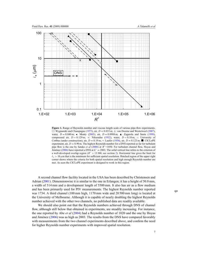
In figure 1, the range of various pipe experiments in terms of the viscous length scale(`∗) as a function of the Reynolds number (R+) is plotted. The experiments include air,compressed air and water as flow medium, but their interrelated relation is a line with theslope −1, according to the relation `∗ = R/R+ and this is independent of the flow medium.As can be seen, most experiments are for low Reynolds numbers. The superpipe covers a widerange of Reynolds numbers but does not pass through the range of interest that was defined insection 2.1; i.e. R+ > 13 300 and `∗ > 10 simultaneously. In the figure, we also plot the rangefor the planned CICLoPE pipe. Although this experiment will have a much smaller Reynoldsnumber range than the superpipe it is designed such that the scales within that range will belarge enough to be reasonably well resolved by present measurement techniques.

3.2. Channel flow experiments

There are two channel flow experiments, at low-to-moderate Reynolds numbers, from whichturbulence data have been reported recently. One is located at the Institute of Fluid Mechanics,Friedrich-Alexander-Universität Erlangen-Nürnberg and detailed specifications can be foundin Zanoun et al (2003). The channel height is 50 mm, its width 600 mm and its length6500 mm. The flow medium is air. Measurements have been reported for Reynolds numbersReτ up to 4783. The results from this facility have relied primarily on hot-wire and pitot probemeasurements, and oil-film interferometry data.

6

Fluid Dyn. Res. 41 (2009) 000000 A Talamelli et al

0.1

1

10

100

1.E+02 1.E+03 1.E+04 1.E+05 1.E+06

R+

* ( m

)

DNS

Figure 1. Range of Reynolds number and viscous length scale of various pipe-flow experiments.�: Wygnanski and Champagne (1973), air, D = 0.033 m; M: van Doorne and Westerweel (2007),water, D = 0.040 m; •: Monty (2005), air, D = 0.0988 m; N: Zagarola and Smits (1998),compressed air, D = 0.129 m; ×: Nikuradse (1932), water, D = 0.10 m; ◦: University ofCottbus (under construction), air, D = 0.19 m; +: Laufer (1954), air, D = 0.123 m; �: CICLoPEexperiment, air, D = 0.90 m. The highest Reynolds number for a DNS reported so far for turbulentpipe flow is the one by Satake et al (2000) at R+=1050. For turbulent channel flow, Hoyas andJiménez (2006) have reported a DNS at h+

= 2003. The solid vertical line refers to the criterion ofa well-developed overlap region (R+ > 13 300, see section 2). Horizontal line gives the limit for`∗ > 10 µm that is the minimum for sufficient spatial resolution. Hatched region of the upper rightcorner shows where the criteria for both spatial resolution and high enough Reynolds number aremet. As seen the CICLoPE experiment is designed to work in this region.

A second channel flow facility located in the USA has been described by Christensen andAdrian (2001). Dimensionwise it is similar to the one in Erlangen; it has a height of 50.8 mm,a width of 514 mm and a development length of 5500 mm. It also has air as a flow mediumand has been primarily used for PIV measurements. The highest Reynolds number reported

Q3was 1734. A third channel (100 mm high, 1170 mm wide and 20 500 mm long) is located atthe University of Melbourne. Although it is capable of nearly doubling the highest Reynoldsnumber achieved with the other two channels, no published data are readily available.

We should also point out that the Reynolds numbers achieved through DNS of channelflow, although still below that obtained in experiments, are steadily increasing. For instance,the one reported by Abe et al (2004) had a Reynolds number of 1020 and the one by Hoyasand Jiménez (2006) was as high as 2003. The results from the DNS have compared favorablywith measurements from the two channel experiments described above, and confirm the needfor higher Reynolds number experiments with improved spatial resolution.

7

Fluid Dyn. Res. 41 (2009) 000000 A Talamelli et al

3.3. Wind tunnel boundary layer experiments

Two closed-return wind tunnels, in which high quality, high Reynolds number boundary layerexperiments have been carried out during the last decade, are the MTL wind tunnel at KTH,

Q4Stockholm and the National Diagnostic Facility (NDF) wind tunnel at the Illinois Institute ofTechnology, Chicago. It is interesting to note that the principal investigators of the turbulentboundary layer studies in these two tunnels (Johansson and Nagib, respectively) have beencooperating, and in some of the resulting publications also used data from both tunnels tostrengthen the line of arguments (see, for instance, Nagib et al 2007, Österlund et al 2000).

The MTL wind tunnel has an overall length of 25 m and test section dimensions of1.2 × 0.8 × 7.0 m3 (width × height × length). The contraction ratio is 9 : 1, a heat exchangercontrols the temperature, and the maximum speed (with empty test section) is 69 m s−1. Forturbulent boundary layer experiments, a flat plate is mounted 20 cm above the tunnel floor,and measurements can be carried out along the full-length of the plate. The leading edge iselliptical and the boundary layer is tripped about 20 cm downstream the leading edge. For highReynolds numbers, the most useful measurement position is at a station 5.5 m downstreamthe leading edge with free stream velocities up to 50 m s−1. Under these conditions, Reθ isapproximately 27 000 and the corresponding δ+ is around 6000.

The NDF at the Illinois Institute of Technology has a 1.52 × 1.22 × 10.3 m3 testsection, and is capable of reaching a maximum free-stream velocity of 110 m s−1 (seealso http://fdrc.iit.edu/facilities/ndf.php). The flow quality is controlled by a honeycomb,six screens and a 6 : 1 contraction upstream of the test section. The resulting free-streamturbulence intensity is <0.05% at all velocities. Turning vanes in two turns of the tunnel areused as heat exchangers for regulating the free-stream temperature, and the turning vanes inone turn are lined with acoustically absorbent material to dampen acoustic disturbances. Thetest section itself is a modular design and its design and long length allow it to be modifiedto establish various pressure gradients (both adverse and favorable) by adjusting the height of17 ceiling panels over the length of the boundary layer plate. The flat plate, which spans thewidth of the test section, measures approximately 10.8 m from the leading edge to the end ofa flap. The plate is suspended 0.52 m above the tunnel floor. Transition triggers in the form of‘V’-notched strips are located between 8 and 25 cm from the leading edge.

Turbulent boundary layer experiments in the NDF have been performed for five differentpressure gradient cases over a flat plate, including the ZPG case (see Nagib et al 2006, 2007).The measurements for all pressure gradient cases were acquired at six streamwise locations;i.e. x = 3.8, 4.6, 5.5, 6.4, 7.3 and 9 m. For the ZPG measurements, the free-stream velocity atthe leading edge was kept at U0 = 30, 40, 50, 60, 70 and 85 m s−1, whereas for the pressuregradient cases upstream free-stream velocities of U0 = 40, 50 and 60 m s−1 were utilized. Thehighest achievable values for ZPG boundary layers in the NDF are Reθ of approximately70 000 and the corresponding δ+ of about 15 000.

In both MTL and NDF tunnels the oil-film interferometry method has been used toobtain an independent measurement of the wall shear stress, whereas various hot-wire andpressure probe measurements have been used for determining the mean and fluctuatingvelocity components.

3.4. Atmospheric boundary layer experiments

The use of the atmospheric boundary layer as a test facility is, of course, an interestingpossibility in order to reach high Reynolds numbers and still have good spatial resolution.Only a few types of terrain are useful if one wants to have a boundary layer over smooth-wall conditions. Measurements from two different types of sites have recently been used for

8

Fluid Dyn. Res. 41 (2009) 000000 A Talamelli et al

boundary layer studies: one site is located in the Utah Great Salt Lake Desert (Kunkel andMarusic 2006), the other measurements are from observations over sea ice in the Antarctic andArctic regions (Andreas et al 2006). There are many difficulties associated with these types ofmeasurements, however, they give access to boundary layers of unprecedented high Reynoldsnumbers. The boundary layer thickness is typically larger than 100 m, whereas free-streamvelocities are of the order of 10–20 m s−1. Hence, the Reynolds number based on boundarylayer thickness is of the order of 108 or larger.

In the experiments of Andreas et al (2006), the idea was to determine the Kármánconstant from measurements in the logarithmic layer. The velocity measurements were madewith propeller and sonic anemometers. In contrast to laboratory experiments, a large numberof profiles were measured under various conditions (wind speed, wind direction, thermalstability, etc) and velocity data from approximately 103 h of measurement time were available.The results show that individual profiles have a large scatter in the values of the Kármánconstant. However, the individual values of the Kármán constant can be averaged and a meanvalue has been reported by the authors. The variation among individual profiles may dependon various reasons; one is probably that the averaging times at each measuring location needto be large in order to achieve good statistical accuracy of the individual mean (see section 6for further discussion about this issue).

On the other hand, Kunkel and Marusic (2006) used hot wires for their measurementsand these experiments have a scope similar to what would be carried out in a wind-tunnelinvestigation. In the Utah desert site it seems harder to get a boundary layer under neutralconditions, and hence, the available measurement time is limited. They present turbulencedata of the streamwise and normal velocity components in the logarithmic layer, as well asspectra that show the −5/3 region over at least two decades in wave number.

4. Research issues for a high Reynolds number flow facility

In the following sections, we will outline a preliminary set of potential scientific objectivesto be investigated at the CICLoPE. The following sample objectives are based onthe outcome from a workshop held in Bertinoro, Italy, during September 2005. Thefull text for the objectives can be found at the homepage of the CICLoPE project(http:// www.ciclope.unibo.it), and the names of some of the key individuals who contributedideas to the objectives are mentioned in the acknowledgment section of this paper.

4.1. Large-scale structures and energy transfer in wall-bounded shear flows

Wall-bounded flows are characterized by a hierarchy of organized eddying motions occurringon different spatial and temporal scales. The near-wall region contains a multitude of quasi-streamwise vortices, which induce organized structures of slow and fast moving fluid. Thekind of structures that populate the outer region is less established. Basically, they aredescribed as packets of hairpin-like vortices, or alternatively as large-scale low-momentumregions, which manifest coherence on scales comparable with the external dimension of theflow. For a long time, there have been suggestions of a coupling between near-wall dynamicsand large structures, and recent numerical simulations seem to confirm this. In this case, near-wall regeneration events would be locked to the specific sites determined by the large-scalestructures and by their slow dynamics.

From a statistical point of view, it is not clear that which kind of mechanism may inducesuch inner–outer scale coupling, leaving open the issue of the origin of the large-scale features.A tool able to deal with this question is provided by the scale-by-scale balance of kinetic

9

Fluid Dyn. Res. 41 (2009) 000000 A Talamelli et al

energy (see e.g. Marati et al 2004). It would discern between the different mechanisms whichmay participate in feeding a given scale of flow motion; namely, local production by couplingwith the mean shear, spatial fluxes and direct/inverse energy cascade across scales.

To further investigate this issue an experiment that guarantees access to widely separatedscales of motion is needed. Various measurement techniques should be used, both standardmethods, such as multipoint hot-wire anemometry but also highly sophisticated measurementtechniques, as for example dual-plane stereo image velocimetry will be useful in this context.

Also the novel technique utilized by Tsuji et al (2007), where fluctuating pressurecan be measured inside the wall-bounded flow, may prove to be very effective here. Thistechnique, which currently is being further developed to increase spatial resolution, givesnew possibilities to study key elements of inner–outer scale interactions through pressureroot mean square (rms)-distributions and their scaling behavior. In addition, but perhapsnot as important, this technique can be used to examine the scaling behavior of two-pointpressure–velocity correlations.

4.2. Anisotropy and SO(3) decomposition

One of the basic aspects of turbulence theory concerns the recovery of isotropy in the small-scale range, which is a real challenge to theoreticians, especially for turbulent wall-boundedflows. Actually, boundary layers display a variety of different behaviors, ranging from theouter part of the logarithmic region, where a classical inertial range is well established,down to the inner part of the log-layer/outer part of the buffer region, where anisotropy maypenetrate within the dissipation scales. This issue has a large impact in all the applicationsthat require simulations of wall-bounded turbulent flows.

In this context, there are still several open questions:

• How is isotropy recovered as a classical inertial range is approached?• Are scaling laws preserved in some generalized sense even in conditions which are

relatively far from purely isotropic conditions?• What are the detailed mechanisms driving the isotropization of the small scales?• Are there aspects of the behavior of the anisotropic scales in the production range which

manifest universality?• Can we develop a theoretical framework to describe the statistics of fluctuations at

production scales?

Recently, the so-called SO(3) decomposition has been applied to gain someunderstanding of part of the issues raised above (see e.g. Jacob et al 2004 and referencestherein). It makes it possible to express structure functions as a sum of components arrangedinto a hierarchy of increasingly anisotropic contributions with the aim of understanding howturbulence changes from anisotropy-dominated fields on the large scales to the isotropy atsmall separations. Most available results deal with mild perturbations of isotropic statistics,but the same theoretical tools can be used to address strongly anisotropic flows as well. Inthis respect, the preliminary evidence from numerical simulations and experiments is stronglyencouraging, though suffering from the shortcoming of facilities unable to explore the finestructure of turbulence at high Reynolds numbers.

4.3. Inner/outer scaling of spectra, correlations and other high-order statistics in variousregions

The spectra of turbulent flows and the correlation functions are very important since they canbe used to separate the effect of different scales, or sizes, of motions that contribute to the

10

Fluid Dyn. Res. 41 (2009) 000000 A Talamelli et al

dispersion of contaminants, the surface friction and the heat transfer from the surface. Suchinformation is essential in developing a better understanding of the underlying physics of theflows and developing accurate predictive models, applicable to the high Reynolds numberflows typical of engineering applications and natural processes.

Measurements have been made of the spectra in a variety of laboratory experimentsand also in the atmospheric boundary layer. Unfortunately, although useful, measurementsfrom these two flows are limited for different reasons. The vast majority of laboratorymeasurements have been limited to moderate Reynolds numbers due to the limited size oftypical facilities. The spatial resolution of measurements at higher Reynolds numbers in thelaboratory is also limited, again due to the limited size of the facilities. One such scalingexperiment at moderately high Reynolds numbers was reported by Österlund et al (2003);however, for the scaling results to be conclusive a larger range of Reynolds numbers wouldbe desirable.

Measurements in the atmospheric boundary layer do not suffer from these limitations andit is possible to attain excellent spatial resolution at very high Reynolds numbers. However,atmospheric measurements are problematic as the experimentalist has no control over the flowconditions, and varying conditions make it difficult to obtain converged statistics.

Accurate scaling experiments hence need a controlled high Reynolds number laboratoryexperiment to eliminate several controversies presently related to the correct scaling of spectraand correlations. Also the scaling of other statistical features of wall-bounded turbulence maybe studied in such a facility, such as the scaling of the turbulence intensity in the bufferregion with Reynolds number (see e.g. Metzger and Klewicki 2001). A high Reynolds numberfacility would also be able to further verify the k−1 spectral law discussed by Davidsonet al (2006).

4.4. Evidence on non-universality of the Kármán constant, and other scaling anomalies

The separation in scale size between the inner, or wall scales, and the outer scales determinedby geometrical constraints increases with the increasing Reynolds number. This separationis what gives the characteristic two-layer feature of wall bounded flows, therefore, in orderto increase our understanding of turbulent flow physics it is essential to obtain accurate datafrom several well-established and documented high-Reynolds number flows. The asymptoticshape of the mean velocity distribution in the overlap region, that connects the inner and outerregions, is a key element in our understanding of wall-bounded turbulence.

Recently completed flat-plate boundary layer experiments at the high Reynolds numbers,Reθ > 10 000, in presence of adverse and favorable pressure gradients, have been used toevaluate the mean velocity profiles in the overlap region (Nagib et al 2006). The profilesexhibit the logarithmic behavior of the mean velocity in the overlap region in a similar wayto the well-documented case of ZPG. In contrast to the ZPG case, the pressure gradient casesexhibit systematic variations in the parameters describing the overlap region, namely, theKármán coefficient κ and the additive term B, which are believed to be constant based onclassical arguments.

The variations in κ and B are not only exhibited for the clearly non-equilibrium cases ofstrong favorable pressure gradient (SFPG; β ≈ −0.15) and complex pressure gradient (CPG),but also for the mild adverse and favorable pressure gradient cases, APG (β ≈ 0.1–0.3) andFPG (β ≈ −0.09–−0.15), respectively. The variations for APG and FPG are opposite innature when referred to the equilibrium state of a ZPG turbulent boundary layer. The resultsare also self consistent and in agreement with fully developed pipe and channel flows whereκ values higher than we find for ZPG are measured; κ ≈ 0.41 compared with 0.384.

11

Fluid Dyn. Res. 41 (2009) 000000 A Talamelli et al

The non-universality of Kármán coefficient κ is not only of scientific importance butalso has a major impact on the prediction of turbulence using various closure models. Allof the currently used models rely on the hypothesis that κ is a constant; often taken to beequal to its most popular value of 0.41. The use of a circular diverging test sections in a pipe-flow experiment, to include ZPG, or converging segments of a ‘pipe’ can be used for furtherconfirmation of these trends.

In addition, the recent high Reynolds number data revealed another limitation of theclassical theory at all finite Reθ values. Nagib et al (2007) suggested after careful assessmentof data over a very wide range of Reynolds numbers, that (at least) two outer length scalesare required to fully describe the mean velocity profile in a ZPG TBL. One can think of thesetwo outer scales as being associated with the boundary layer thickness and the streamwisegrowth of the boundary layer thickness. They suggest that it is only at infinite Reynoldsnumbers that the ZPG TBL reduces to a two-scale problem with one inner scale and oneouter scale as in the classical theory. In contrast, a fully developed pipe flow is homogeneousin the streamwise direction, and should therefore, insure a single outer scale and the uniqueopportunity to examine other asymptotic trends of the mean flow at finite but high Reynoldsnumbers.

4.5. Small deviation of canonical scaling laws using approximate symmetries/Lie groups

In recent years, it became clear that at least for ‘clean’ canonical turbulent flows, such aspipe, channel or boundary layers, the group theory provides the axiomatic building blockfor deriving turbulent scaling laws. The basis of the analysis is the infinite set of multipointcorrelation equations that solely originate from the Navier–Stokes equations. Applying grouptheory invariant solutions (scaling laws in turbulence) for wall-bounded shear flows havebeen obtained without any closure assumption. In fact, it turned out that the von Kármánlogarithmic law of the wall is by no means the only nontrivial self-similar mean velocityprofile which may be given explicitly. The set of mean velocity profiles obtained includesan algebraic law in the center of a channel flow, the linear mean velocity in the center ofa Couette flow, the linear mean velocity in the center of a rotating channel flow and anexponential mean velocity profile. The exponential law in particular has not been previouslyreported in the literature. Besides the original work of Oberlack (2001) it is shown by Lindgrenet al (2004), using the high Reynolds number KTH data base as well as DNS data in Khujadzeand Oberlack (2004), that such a law describes the outer part of a boundary layer flow over aflat plate and is, in fact, an explicit form of the velocity defect law.

All the latter classical and new scaling laws were, however, derived under idealized andrather ‘clean’ conditions. In particular, infinite Reynolds number and the absence of a pressuregradient was presumed. Further, a fully parallel flow in the mean sense was conjectured whichis not true for boundary layer flows.

For almost two decades Reynolds number dependence of turbulent scaling laws has beenunder intense debate and, in fact, recently also pressure-gradient dependence and non-paralleleffects have been observed (see Nagib et al 2006). Though these effects appear to be ofhigher order, i.e. they may not change the global functional behavior of the scaling laws theystill significantly influence the scaling parameter such as the von Kármán constant κ in thelogarithmic law of the wall.

A new development is to introduce approximate group theory to derive the turbulentscaling laws which may depend on a small parameter such as those mentioned above.Approximate groups provide a new mathematical methodology which unifies group theorywith regular asymptotics. Hence, it gives the ideal framework to tackle tasks, e.g. to derive the

12

Fluid Dyn. Res. 41 (2009) 000000 A Talamelli et al

Figure 2. Comparison between cross-section area of pipe and channel flow. A channel with anaspect ratio of 12 has a cross section which is 15 times larger than a corresponding pipe flow.

pressure-gradient dependence of the von Kármán constant κ . The key advantage of the newmethod is that certain physical parameters such as the pressure gradient, which are underidealized conditions are symmetry breaking, i.e. no exact scaling law exists, can now bemathematically handled at least in an asymptotic sense.

In order to thoroughly validate these types of scaling laws for both the effect of pressuregradient and Reynolds number dependence, high Reynolds number experimental data areneeded.

5. Design features of pipe-flow facility at CICLoPE

The idea of a collaboration between several researchers from different universities on a highReynolds number flow facility located in Predappio was conceived during a visit by HassanNagib and Alessandro Talamelli to KTH in 2004. As seen in section 3, many attempts havebeen made to create large-scale experiments but so far they have been limited in one wayor the other. The use of a pipe as compared with, for instance, a parallel-walls channel isadvantageous in two ways, both with respect to the cost of construction and the flow rateneeded. Recent channel flow experiments have used aspect ratios around 1:12 in order toensure a sufficiently wide central region without the influence from the side walls. Such achannel has a cross-stream area about 15 times larger than a pipe with a diameter of thesame dimension as the channel height. Hence, to obtain the same Reynolds number basedon diameter or height the flow rate would have to be some 15 times larger in the case of thechannel (see figure 2). Also, the construction costs and space requirements would increasenearly proportionally in case of the channel.

5.1. Special requirements for a long-pipe-flow experiment

The design of a long-pipe-flow facility is non-standard and a large number of requirementshas to be met. In the following, we describe various criteria and discuss the design featuresof the facility as they are known today (May 2007). In principle, a long pipe flow facilitycan be designed in a similar way as a wind tunnel. However, there are two main differences:the pressure drop is much larger in the test section and the pipe is in itself the test section.These characteristics put extra demands both on the fan, which has to provide the desiredflow rate against a higher pressure drop, and on the pipe itself which must satisfy some strictrequirements, e.g. geometric tolerances, surface finish and alignment.

5.2. The laboratory

The laboratory for CICLoPE is located in Predappio, Italy, besides the old factory of theCaproni Industry, which was one of the major sites of aircraft production during the period1930–1945. The site in Predappio was built after the First World War to improve theairplane production in Italy, and it became operative in 1935. After 1940, it was successivelyimproved in order to boost its productivity and fulfill the needs during the Second World

13

Fluid Dyn. Res. 41 (2009) 000000 A Talamelli et al

Figure 3. Outline of the long-pipe facility. Figures clockwise from upper left. a) Full-length of thepipe located in the tunnel, (b) close-up of the third and fourth corners and the contraction beforethe start of the pipe, (c) cross section of the pipe facility and the tunnel showing the third and fouthcorners and (d) the end of the pipe with the diffuser and test section.

War. It was during this period that a tunnel complex was excavated, in order to provideboth shelter for civilians, and make the plant operative even under bombing activities. After1944, the Predappio site was gradually vacated and all the equipments moved to sites locatedfarther north. The tunnels were subsequently occupied by Allied forces until 1946 and thenfinally transferred to the Italian Aeronautica Militare. In 2006, the tunnels were given to theUniversity of Bologna specifically for the CICLoPE laboratory.

The complex comprises two 130 m long tunnels with a diameter of about 9 m each. Thetwo tunnels are linked together and to the exterior by two perpendicular galleries of a smallersize. The space available in these tunnels is not restricted to the long-pipe experiment, butallows enough room for future developments and for other experiments. The section of thefirst tunnel is separated in two floors. The long-pipe facility will be set on the upper floor andthe return circuit will be located under the ground floor of the tunnel as shown in figure 3.This layout has been chosen as the best compromise in terms of cost, accessibility, securityand space for future developments.

5.3. The facility

The present configuration of the experimental set-up is the result of a preliminary designphase. Hence, some elements could still change in terms of dimensions and material until theend of the final construction. The facility is basically a closed-loop wind tunnel operatingwith air at atmospheric pressure. A closed loop has been chosen since it will allow the

14

Fluid Dyn. Res. 41 (2009) 000000 A Talamelli et al

flow characteristics to be accurately controlled. The layout resembles an ordinary windtunnel where the main difference is the long test section which gives most of the frictionlosses. However, many of the various aerodynamic components are the same as those foran ordinary wind tunnel (corners, diffusers, screens, contraction, etc), and for several ofthese components we relied on the recent experience gained when constructing the MTLand BL-wind tunnels at KTH Mechanics, Stockholm. In the following, we describe thefacility starting downstream of the test section and following the flow loop around the circuit(again see figure 3).

The expansion part linking the test section to the return flow section will have twoexpanding corners of rectangular cross section with an expansion ratio of 1.3 based on thedesign of Lindgren et al (1998). This will achieve a substantial part of the required totalexpansion of the flow already by the beginning of the lower return duct. After the secondcorner, a two-dimensional diffuser expands the flow laterally to the full width along a returnsection. At the end of this return section, a two-dimensional contraction followed by a squareto circular converter brings the air into the fan.

A heat exchanger located at the end of the return flow section just upstream of thecontraction, where the mean air velocity is the lowest, will accurately control the airtemperature in the pipe. The mixing produced by the fan will ensure a thermal homogeneityof the flow after the heat exchanger. The aim is to keep the flow temperature variation in thetest section less than 0.1 ◦C.

The fan is of the single-stage type, with a diameter of 1.8 m, and has 12 blades specificallydesigned for this experiment. The fan is designed to produce 3.5 kPa of pressure differencewith a volume flow rate of 38 m3 s−1. It will be powered by a 250 kW ac-motor controlledby a frequency converter for accurate velocity control. The section between the fan and thesettling chamber will have a circular cross section of constant area. A 11 m long straightpipe downstream of the fan will be coated with noise absorbing material to reduce the noiseproduced by the fan and to allow the wake of the fan to decay before the corner.

The two last corners are non-expanding with circular cross sections, and are separatedby a straight fiberglass tube. Finally, the settling chamber and contraction will be madeof fiberglass, and will incorporate a honeycomb and three screens to homogenize theflow before the settling chamber, and to reduce the turbulence intensity. The shape of thecontraction will be similar to the one used in the MTL wind tunnel, which was designed usinginviscid/boundary layer calculations to optimize the pressure gradient along the contractionwalls. The contraction will have a length of 2.6 m and a contraction ratio of four withdiameters of 1.8 and 0.9 m for the inlet and outlet, respectively.

The main part of the set up is the long pipe. It consists of a 115 m long tube with an innerdiameter of 0.9 m. The pipe will be made of 5 m long modules held on concrete blocks byprecision positioning elements. The pipe modules are made of carbon fiber with flanges atboth ends for precise junction of the elements. The main test section, at the end of the pipe,will have optical access for PIV and local density approximation (LDA) as well as varioustraversing systems for different sensor types.

5.4. Pressure drop

The distribution of the pressure drop along the circuit is shown in table 1 and thecorresponding power factor is shown in table 2. As it can be seen, 78% of the pressure dropis generated by the friction in the pipe, which also makes the power factor quite high ascompared to the value for a typical wind tunnel. The total pressure drop in the circuit is about3500 Pa at a mean velocity of 60 m s−1 in the pipe.

15

Fluid Dyn. Res. 41 (2009) 000000 A Talamelli et al

Table 1. Percentage of pressure losses at a 50 m s−1.

Element % losses

Main pipe 78.04Section converter 1.19Corner 1 (expanding) 2.25Vertical diffuser 1.93Corner 2 (expanding) 0.47Two-dimensional diffuser 1.09Return duct 1.62Cooling system 0.16Two-dimensional convergent 0.02Section converter 0.08Circular pipe 0.25Corner 3 0.18Vertical part 0.07Corner 4 0.18Honeycomb 0.25Screens 11.64Settling chamber 0.01Contraction 0.54

Table 2. Power factor.

U (m s−1) Power factor at various mean velocities

5 2.5215 1.9630 1.7545 1.6760 1.61

5.5. Critical requirements

5.5.1. Surface roughness. The mechanical requirements for the pipe are mainly fixed bythe demand to have a hydrodynamically smooth surface. In order to achieve this, the sandequivalent surface roughness of the pipe ks has to be lower than 3.5`∗ according to recentresults by Shockling et al (2006) for a honed finished surface. They also showed that for sucha surface ks/krms ' 3. As specified earlier the minimal scale for spatial resolution for the longpipe is `∗ = 10 µm, which translates into an rms surface roughness of maximum 12 µm. Withthe proposed carbon fiber pipe modules the surface roughness will be well below this value.

5.5.2. Diameter accuracy. The absolute accuracy of the pipe diameter is not very stringentas long as its variations are small along the pipe. High-flow-quality wind tunnels such as MTLat KTH in Stockholm or NDF at IIT Chicago have mean velocity variations 1U/U0 of theorder of 0.2%. For a pipe flow one can write

1U

U0=

1S

S= 2

1D

D, (5)

where S is the cross-section area of the pipe and D its diameter. To get similar flow quality,the diameter variation for a diameter of 0.9 m is

1D 61U

U0

D

2= 0.9 × 10−3 m. (6)

16

Fluid Dyn. Res. 41 (2009) 000000 A Talamelli et al

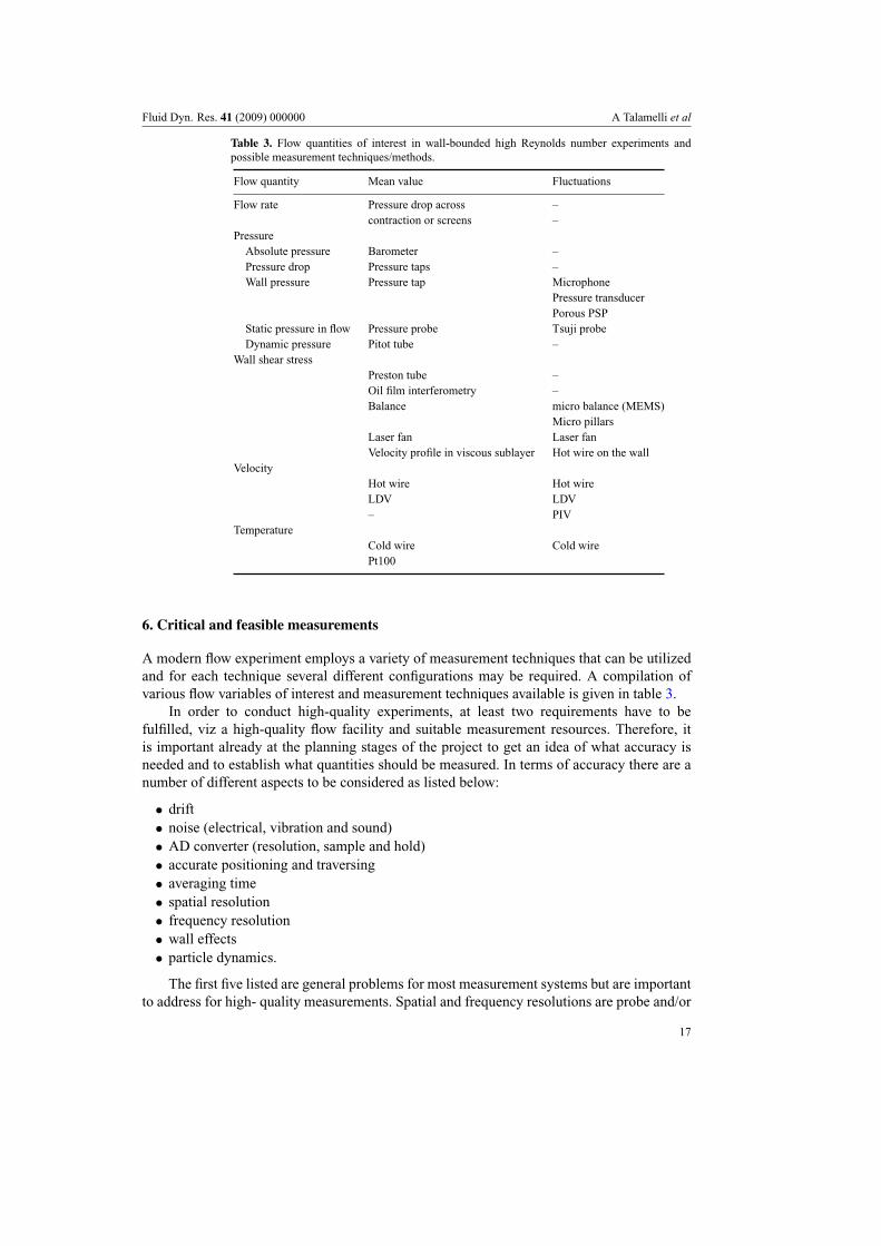
Table 3. Flow quantities of interest in wall-bounded high Reynolds number experiments andpossible measurement techniques/methods.

Flow quantity Mean value Fluctuations

Flow rate Pressure drop across –contraction or screens –

PressureAbsolute pressure Barometer –Pressure drop Pressure taps –Wall pressure Pressure tap Microphone

Pressure transducerPorous PSP

Static pressure in flow Pressure probe Tsuji probeDynamic pressure Pitot tube –

Wall shear stressPreston tube –Oil film interferometry –Balance micro balance (MEMS)

Micro pillarsLaser fan Laser fanVelocity profile in viscous sublayer Hot wire on the wall

VelocityHot wire Hot wireLDV LDV– PIV

TemperatureCold wire Cold wirePt100

6. Critical and feasible measurements

A modern flow experiment employs a variety of measurement techniques that can be utilizedand for each technique several different configurations may be required. A compilation ofvarious flow variables of interest and measurement techniques available is given in table 3.

In order to conduct high-quality experiments, at least two requirements have to befulfilled, viz a high-quality flow facility and suitable measurement resources. Therefore, itis important already at the planning stages of the project to get an idea of what accuracy isneeded and to establish what quantities should be measured. In terms of accuracy there are anumber of different aspects to be considered as listed below:

• drift• noise (electrical, vibration and sound)• AD converter (resolution, sample and hold)• accurate positioning and traversing• averaging time• spatial resolution• frequency resolution• wall effects• particle dynamics.

The first five listed are general problems for most measurement systems but are importantto address for high- quality measurements. Spatial and frequency resolutions are probe and/or

17

Fluid Dyn. Res. 41 (2009) 000000 A Talamelli et al

instrument dependent, whereas wall effects are problems arising from interference betweenthe wall and the probe. For intrusive methods (i.e. probe measurements), it is not only theprobe interference that may constitute an error source but also the blockage of the traversingsystem may also result in disturbances. The question whether particles follow the flowaccurately is, however, a question only for non-intrusive methods which use the particlesto determine the flow speed.

Earlier turbulence research has mostly relied on point measurements, i.e. measurements atone point at a time, whereas for many situations two or multipoint measurements are needed.With PIV also field measurements in a plane are possible and with stereoscopic PIV all threevelocity components can be measured simultaneously.

For measurements using indirect measurements, such as hot-wire anemometry, theaccuracy of the measurements cannot be higher than the accuracy of the calibration whichimplies that the calibration set-up is as important as the measurements themselves and has tobe designed accordingly.

The standard quantities that should be considered in a turbulence experiment shouldcomprise the following quantities and distributions of all three velocity components:

• mean velocity distribution

• turbulence intensity (rms) distribution

• distribution of higher moments

• probability density distributions (pdf)

• spectra (wave number and frequency)

• correlations (spatial and time).

To ensure the desired accuracy in the results, it will be essential to have and perhaps touse at the same time complementary means for measuring mean and turbulence quantities.

6.1. Spatial resolution issues

The accuracy and representation of all measurement techniques are dependent on what maygenerally be referred to as the probe size or volume. Velocity measurements using hot wires,LDV, PIV and other methods are particularly affected by such spatial averaging or resolution.

For single hot wires, it is the length of the hot-wire sensor which is the critical dimension,and the smallest probes which are convenient to use have a wire length of the order of 250 µmwith a sensor diameter of 1.2 µm. However, it is possible to use wires with a diameter of0.6 µm, thereby allowing us to reduce the length to 120 µm. Various studies have shown thatprobes with a spanwise length larger than about 10`∗ lead to spatial averaging effects, whichindicates that the smallest viscous length should be larger than about 10 µm in order to beable to resolve the turbulence without significant effects of spatial averaging.

Another approach to accurately measure averaged quantities relies on repeatedmeasurements with probes of different small sensing elements and extrapolation of the datadown to much smaller scales. i.e. the desired quantity can be measured with several probesof different but not too large sensing lengths and then the results are extrapolated to azero sensing element size. The extrapolation can become quite accurate if it is combinedwith theoretical knowledge about the effect of the spatial averaging. Even time-resolvedmeasurements can be corrected if such measurements are carried out simultaneously (invirtually the same position) with two probes of different spatial extent. This may be hardto achieve but could be tried with for instance two parallel hot wires.

18

Fluid Dyn. Res. 41 (2009) 000000 A Talamelli et al

6.2. Time-averaging issues

When averaging a stationary turbulent signal the accuracy of the average depends on theaveraging time (see, for instance, Sreenivasan et al 1978). It is possible to show that therelative error (ε) for the determination of the mean value becomes

ε =

(23

T

)1/2 urms

U, (7)

where 3 is the integral timescale of the turbulence. This result gives a useful estimate ofhow long we need to sample in order to get a specified accuracy. For instance if we want anaccuracy better than 1% we should sample for at least

T (ε < 1%) > 23

(urms

U

)2

× 104.

As an example, consider measurements of the streamwise velocity at various radii in aturbulent pipe flow experiment with air as the flowing medium and with UCL = 30 m s−1.The diameter (D = 2R) of the pipe is 0.9 m. The maximum local level of urms/U is 0.40,which occurs within the viscous sublayer close to the wall. The integral length scale is of theorder of the pipe radius and a typical propagation speed may be taken as half the centerlinevelocity. This gives an estimate of the integral timescale as 2R/UCL=0.03 s. For ε to becomesmaller than 1% everywhere, we find that T has to be larger than 100 s. On the other hand, ifthe mean velocity should only be determined at the centerline itself, the turbulence intensityis there only about 4%, and the required sampling time would be a factor hundred less!

Similar result for higher moments can also be obtained and for the second moment, i.e.u2

rms, we have

ε2(u2) = 23

T

[(u4)

(u2)2 − 1

]= 2

3

T(F − 1),

where F is the flatness factor. If u can be assumed Gaussian, then F = 3 and we obtain

ε2(u2) = 43

T.

The results show that to obtain urms with an error less than 1%, we need a samplingtime longer than 40 0003 which in the pipe-flow experiment with air mentioned above wouldrequire 1800 s or 30 min for measurements in the viscous sublayer. For higher moments, thesampling time will be even longer to obtain the similar accuracy.

These examples clearly show that in order to obtain high accuracy results in a largefacility it is of utmost importance to be able to have stationary and drift-free conditions bothfor the facility itself and the measurement equipment. When measurements are made at lowvelocities, this issue becomes even more critical since the averaging time must increase toobtain the same statistical accuracy, hence the time-averaging issue is opposite to that of theprobe resolution.

7. Conclusions

Simulations of turbulence are regularly moved to the largest and most expensive computersworldwide, but are still far from replicating the high Reynolds numbers found in nature andvarious critical technologies. Experiments, on the other hand, are still usually made under

19

Fluid Dyn. Res. 41 (2009) 000000 A Talamelli et al

rather primitive conditions and using fairly small-scale facilities, typically involving only onelaboratory or research group. The need for a large-scale collaborative experimental effortin order to address and resolve several critical research issues within the turbulence area ishopefully evidenced from the present paper. The fully developed turbulent pipe flow is anideal configuration to study high Reynolds number turbulence where homogeneous conditionscan be achieved experimentally with relative ease. The CICLoPE project may be a first steptoward a new approach on how to carry out experimental turbulence research in the future.

Acknowledgments

We acknowledge the input from Carlo Casciola and Renzo Piva (Università di Roma ‘LaSapenzia’), Martin Oberlack and Michael Frewer (TU Darmstadt), Ivan Marusic (Universityof Melbourne) and Timothy B Nickels (Cambridge University) who, in connection withthe workshop in Bertinoro in September 2005, formulated the research issues discussed insection 4. Dr Ines Fabbro from the University of Bologna and Dr Marina Flamigni fromProvincia di Forli for the invaluable work concerning the transfer of the properties of thetunnel complex and the project funding. Dr Gianluca Piraccini, Dr Maurizio Tappi, Mr PaoloProli and Alessandro Rossetti are also thanked for their contribution during the design phaseof the pipe. The KTH group thanks the Swedish foundation for international cooperation inresearch and higher education (STINT) for providing a grant for cooperation between KTHand the University of Bologna.

References

Abe H, Kawamura H and Matsuo Y 2004 Surface heat-flux fluctuations in a turbulent channel flow up to Reτ = 1020with Pr = 0.025 and 0.71 Int. J. Heat Fluid Flow 25 404–19

Andreas E L, Claffey K J, Jordan R E, Fairall C W, Guest P S, Persson P O G and Grachev A A 2006 Evaluations ofthe von Kármán constant in the atmospheric surface layer J. Fluid Mech. 559 117–49

Christensen K T and Adrian R J 2001 Statistical evidence of hairpin vortex packets in wall turbulence J. Fluid Mech.431 433–43

Coles D E and Hirst E A 1969 Computation of turbulent boundary layers —1968 AFOSR-IFP-Stanford Conferencevol 2 Stanford University

Q5Davidson P A, Nickels T B and Krogstad P-A 2006 The logarithmic structure function law in wall-layer turbulence

J. Fluid Mech. 550 51–60Hoyas S and Jiménez J 2006 Scaling of the velocity fluctuations in turbulent channels up to Re = 2003 Phys. Fluids

18 011702Jacob B, Biferale L, Iuso G and Casciola C M 2004 Anisotropic fluctuations in turbulent shear flows Phys. Fluids

16 4135–42Khujadze G and Oberlack M 2004 DNS and scaling laws from new symmetry groups of ZPG turbulent boundary

layer flow Theoret. Comput. Fluid Dyn. 18 391–411Knobloch K and Fernholz H 2004 Statistics, correlations, and scaling in a turbulent boundary layer at Reδ2 6

1.15 × 105 IUTAM Symp. Reynolds number scaling in turbulence, Princeton University, USA, 11–13 September(Dordrechr: Kluwer) p 11

Kunkel G J and Marusic I 2006 Study of the near-wall-turbulent region of the high-Reynolds-number boundary layerusing an atmospheric flow J. Fluid Mech. 548 375–402

Laufer J 1954 The structure of turbulence in fully developed pipe flow NACA Report 1174Lindgren B, Österlund J and Johansson A V 1998 Measurement and calculation of guide vane performance in

expanding bends for wind-tunnels Exp. Fluids 24 265–72Lindgren B and Johansson A V 2004 Evaluation of a new wind tunnel with expanding corners Exp. Fluids 36 197–203

Q5Lindgren B, Österlund J M and Johansson A V 2004 Evaluation of scaling laws derived from Lie group symmetry

methods in zero-pressure-gradient turbulent boundary layers J. Fluid Mech. 502 127–52Marati N, Casciola C M and Piva R 2004 Energy cascade and spatial fluxes in wall turbulence J. Fluid Mech.

521 191–215

20

Fluid Dyn. Res. 41 (2009) 000000 A Talamelli et al

McKeon B J, Li J, Jiang W, Morrison J F and Smits A J 2004 Further observations on the mean velocity distributionin fully developed pipe flow J. Fluid Mech. 501 135–47

Metzger M M and Klewicki J C 2001 A comparative study of near-wall turbulence in high and low Reynolds numberboundary layers Phys. Fluids 13 692–701

Monty J P 2005 Developments in smooth wall turbulent duct flows PhD Thesis Department of Mechanic andManufacturing Engineering, University of Melbourne

Nagib H M, Chauhan K A and Monkewitz P A 2005 Scaling of high Reynolds number turbulent boundary layersrevisited AIAA paper 2005–4810

Q5Nagib H M, Christophorou C and Monkewitz P A 2006 High Reynolds number turbulent boundary layers subjected to

various pressure-gradient conditions ‘IUTAM Symposium on One Hundred Years of Boundary Layer Research:Proc. IUTAM Symposium DLR-Göttingen, Germany, 12–14 August 2004’ (Berlin: Springer) pp 383–94

Nagib H M, Chauhan K A and Monkewitz P A 2007 Approach to an asymptotic state for ZPG turbulent boundarylayers Phil. Trans. R. Soc. A 365 755–70

Nickels T B, Maurusic I, Hafez S and Chong M S 2005 Evidence of the k−11 law in a high-Reynolds-number turbulent

boundary layer Phys. Rev. Lett. 95 074501Nikuradse J 1932 Gesetzmässigkeit der turbulenten Strömung in glatten Rohren Forschg. Arb. Ing.–Wes. 356Oberlack M 2001 A unified approach for symmetries in plane parallel turbulent shear flows J. Fluid Mech.

427 299–328Österlund J M, Lindgren B and Johansson A V 2003 Flow structures in zero pressure-gradient turbulent boundary

layers at high Reynolds numbers Eur. J. Mech. 22 379–90Österlund J M, Johansson A V, Nagib H M and Hites M H 2000 A note on the overlap region in turbulent boundary

layers Phys. Fluids 12 1–4Satake S, Kunugi T and Himeno R 2000 High Reynolds number computation for turbulent heat transfer in a pipe flow

High Performance Computing (Lecture Notes in Computer Science vol 1940) (Berlin: Springer) pp 514–23Shockling M A, Allen J J and Smits A J 2006 Roughness effects in turbulent pipe flow J. Fluid Mech. 564 267–85Sreenivasan K R, Chambers A J and Antonia R A 1978 Accuracy of moments of velocity and scalar fluctuations in

the atmospheric surface layer Bound. Layer Meteorol. 14 341–59Tsuji Y, Fransson J H M, Alfredsson P H and Johansson A V 2007 Pressure statistics in high Reynolds number

turbulent boundary layer J. Fluid Mech. 585 1–40van Doorne C W H and Westerweel J 2007 Measurement of laminar, transitional and turbulent pipe flow using

stereoscopic-PIV Exp. Fluids 42 259–79Wygnanski I J and Champagne F H 1973 On transition in a pipe. Part 1. The origin of puffs and slugs and the flow in

a turbulent slug J. Fluid Mech. 59 281–335Zagarola M V and Smits A J 1998 Mean-flow scaling of turbulent pipe flow J. Fluid Mech. 373 33–79Zanoun E-S, Durst F and Nagib H 2003 Evaluating the law of the wall in two-dimensional fully developed turbulent

channel flows Phys. Fluids 15 3079–89

21

QUERY FORM

Journal: fdr

Author: A Talamelli et al

Title: CICLoPE—a response to the need for high Reynolds number experiments

Article ID: fdr303072

Page 1

Q1.Please specify and provide the e-mail address of the corresponding author.

Q2.Please update.

Page 6

Q3.Please define PIV.

Page 7

Q4.Please define MTL.

Page 20

Q5.Please cite references Coles DE and Hirst E A 1969, Lindgren B and Johansson A V 2004and Nagid et al 2005 at appropriate places in the text.

Reference linking to the original articles

References with a volume and page number in blue have a clickable link to the original article created from datadeposited by its publisher at CrossRef. Any anomalously unlinked references should be checked for accuracy. Palepurple is used for links to e-prints at ArXiv.