Aid and Fertility

Dany Bahar

CID Graduate Student and Research Fellow Working Paper No. 38, May 2009

© Copyright 2009 Dany Bahar and the President and Fellows of Harvard College

at Harvard UniversityCenter for International DevelopmentWorking Papers

Aid and Fertility

Citation, Context and Program Acknowledgements

This paper may be cited as:

Bahar, Dany. “Aid and Fertility” CID Graduate Student Working Paper

Series No. 38, Center for International Development at Harvard University,

May 2009. Available at http://www.cid.harvard.edu/cidwp/grad/038.html.

Professor Ricardo Hausmann has approved this paper for inclusion in the

Graduate Student and Research Fellow Working Paper Series. Comments

are welcome and may be directed to the author.

Aid and Fertility ∗

Dany Bahar †

May 22, 2009

Abstract

This paper uses a panel data from developing countries to study

the relationship between foreign aid flows and fertility rates. By mak-

ing use of natural disasters in neighboring countries as an instrumental

variable to foreign aid receipts,I find that a percentage point increase

in the share of aid in the GDP increases on average fertility rates

among the population by 0.045 additional children. This can be trans-

lated to an additional child for about every 22 women of childbearing

age. The positive effect of foreign aid on fertility rates can contribute

to the current debate on foreign aid, and supply an additional expla-

nation for its limited efficacy historically. By making use of the same

instrumental variable, I also find no effect of foreign aid on other de-

terminants of economic growth and growth itself.

Keywords: Foreign Aid, Aid Flows, Fertility Rate, Growth, Economic

Growth, Economic Development

JEL Codes: O11, O16, F35, J13

∗I would like to thank Omer Moav and Eric Gould from the Economics Departmentat the Hebrew University of Jerusalem (HUJI) for their academic guidance and advise.Thanks to Roy Mill for fruitful discussions. The original version of this research waspresented as the thesis requirement for opting the M.A. degree in Economics at the HUJIin June 2008.

†Harvard University - Kennedy School of Government; Hebrew University - EconomicsDepartment. dany bahar@hks10.harvard.edu

1

1 Introduction

In recent years the world witnessed a public debate on whether foreign aid

is in fact contributing to ending poverty or speeding up economic growth

among developing countries. Jeffrey Sachs (2005) in his book “The End of

Poverty” presents an analysis of the low cost investments needed (i.e. foreign

aid) per individual in order to overcome malaria, hunger and other extreme

poverty factors mainly in Africa. Sachs argues that the goals presented in

the UN Millennium Assembly are fully achievable by increasing the financial

assistance of the west toward developing countries.

The other side of the coin is presented by William Easterly (2006) in his

book “The White Man’s Burden: Why the West’s Efforts to Aid the Rest

Have Done So Much Ill and So Little Good”. In Easterly’s views, the failure

in reaching these goals is not related to low foreign aid transfers, but to

bad planning. Moreover, Easterly raises the question: if indeed the costs of

ending poverty are so low, how come development agencies were not able to

significantly lower poverty rates after all the enormous amounts of financial

resources invested until now?

The debate on the effectiveness of foreign aid has been present among

economists for decades. Academic literature about foreign aid data back

to the mid fifties. Milton Friedman attacked foreign aid by arguing that

politicians will not allocate aid efficiently resulting in the political elite ben-

efiting from aid flows (Friedman, 1958). Later, several studies tried to study

the relationship between foreign aid and saving rates or economic growth

mainly ignoring endogeneity problems,1 still without reaching a single and

clear conclusion.

However, only during the past decade economists started to estimate

the causal effect of foreign aid on economic growth by dealing with endo-

geneity issues. Peter Boone (1996) reopened the debate by estimating the

1Papanek (1973), Mosley et. al. (1987)

2

effect of foreign aid on public and private consumption and investment. He

found that aid does not significantly increase investment, nor benefit the

poor (measured by lack of improvements in human capital indicators like in-

fant mortality). Also, the impact of aid does not vary according to whether

recipients are liberal-democratic governments or highly repressive regimes.

However, ceteris paribus, more democratic regimes have 30 percent lower in-

fant mortality. Hence, Boone suggests that short term aid should be targeted

to support new liberal regimes, which might be more successful in achieving

mid and long term economic goals.

A few years later, Burnside and Dollar (2000) showed that foreign aid has

a significant positive impact on growth whenever “good policies” are present.

They did this by finding a significant positive estimator of the interaction

term between aid and a “good policies” index in their empirical specifica-

tion. However, Easterly (2004) showed how the interaction term becomes

insignificant when expanding the sample used by Burnside and Dollar and

maintaining their same specification.

Hansen and Tarp (2001) found that by adding the aid parameter both

in its linear and quadratic form to the growth equation, aid has a positive

impact on growth showing with diminishing results. In their findings, the

square of aid drives out the good policies interaction term of Burnside and

Dollar. In addition, they found that when controlling for investment and

human capital, there is no effect of aid on growth, meaning that aid affects

growth through capital accumulation, both physical and human.

A number of other studies, motivated by Burnside and Dollar, changed

the latter specification, resulting again in inconclusive results.2 Roodman

(2007) makes a very complete review of the literature and explore the fragility

of several studies of aid and growth. He finds that the results in all these

empirical studies are not robust to slight changes in their specifications or

2Guillaumont and Chauvet (2001), Collier and Dehn (2001), Collier and Dollar (2002,2004),Collier and Hoeffler (2004) and Dalgaard, Hansen and Tarp (2004).

3

extensions of their datasets.

Nevertheless, the attention of most economists studying foreign aid has

been concentrated mostly on economic growth, ignoring other variables which

might have a direct impact on the latter. Analyzing the effect of aid on the

determinants of growth, separately, might help us to find complementary

explanations to the limited efficacy of foreign aid flows. This empirical paper

will focus on the fertility rates of the developing countries and how do they

respond to foreign aid.

Already in the early seventies, the ecologist and microbiologist Garret

Hardin wrote about possible consequences of foreign aid and linked it to

population growth. Hardin (1974) criticizes the idea of creating a “World

Food Bank” (i.e. food aid) by explaining that if poor countries know that

they will be provided with nourishment in times of emergency, they will not

have an incentive to manage properly their food reserves. It will also back

away their capacity to self-sustain themselves, thus staying poor forever. He

links aid to population growth as follows:

“If poor countries received no food from the outside, the rate

of their population growth would be periodically checked by crop

failures and famines. But if they can always draw on a world

food bank in time of need, their population can continue to grow

unchecked, and so will their “need” for aid. In the short run, a

world food bank may diminish that need, but in the long run it

actually increases the need without limit.”

In fact, Malthus (1978) already made a similar argument using income

in place of food. In times of economic prosperity, couples will tend to marry

earlier, have more children and thus countries will experience higher popula-

tion growth rates. More recent economic models can also be used to explain

this phenomenon and they may explain how aid can be translated to higher

fertility rates if it is perceived by household as non-wage income or even

subsidies in prices. These models are explored further in the next section.

4

Actually, many forms of foreign aid are actually distributed among the

poor population as cash transfers or subsidies on prices (like food aid) as

a short-term alleviating measure. In its official website3, the United States

Agency for Foreign Aid (USAID) specifies:

“The United States is the world’s largest food aid donor and pro-

vides approximately half of all food aid to populations throughout

the world. In recent years, the USG (US Government) has pro-

vided approximately $1 billion through the U.N. World Food Pro-

gram (WFP), or approximately 40 percent of all contributions to

the organization. The USG contributes significant international

food aid through non-governmental organizations. The USG also

looks to other donors to provide food aid to populations in need.”

A BBC press article titled “Ethiopia’s food aid addiction” (February,

2006) links food aid to the ineffectiveness of aid by arguing:

“Like a patient addicted to pain killers, Ethiopia seems hooked

on aid. For most of the past three decades, it has survived on

millions tonnes of donated food and millions of dollars in cash.

It has received more emergency support than any other African

nation in that time. Its population is increasing by 2m every

year, yet over the past 10 years, its net agricultural production

has steadily declined.”4

Similarly, a press article of the Associated Press on June 2008 titled “Food

aid saves millions but world hunger lingers”5 also testifies that, in spite of

food aid reaching millions of people in starvation during the last years, the

failure of the agriculture in poor regions is keeping developing countries from

ensuring enough food for their own people.

3http://www.usaid.gov/our work/humanitarian assistance/foodcrisis/4http://news.bbc.co.uk/2/hi/africa/4671690.stm5http://a.abcnews.com/International/wireStory?id=4976888

5

Economic literature on the possible link between foreign aid and fertility

rates is scarce.6 Nevertheless, for economists exists a strong motivation to

study this possible relationship. If in fact foreign aid is having a positive

impact on fertility rates and population growth, this could be diluting cap-

ital per capita, and hence inhibiting economic growth of the aid recipient

countries.

Using country-level panel data, I find a significant and positive effect of

foreign aid on fertility rates. On average, a percentage point increase in

foreign aid as a share of the GDP will increase the fertility rates on approxi-

mately 0.045 children per woman of childbearing age, meaning an additional

child for approximately every twenty two women. These results represent

a causal relation, computed using a two stages least squares estimator us-

ing natural disasters in neighboring countries as an instrumental variable to

foreign aid flows.

The results of this job can contribute to two controversial debates cur-

rently taking place. The first is related to find feasible explanations to the still

high fertility rates across poor countries, in particular, in the Sub-Saharan

Africa region. The second relates to the long-standing debate about the ef-

fectiveness of foreign aid, opening a new debate on studying the effect of

the latter not only on growth rates, but in other determinants of economic

prosperity.

The remainder of this paper is organized as follows. The next section

contains an overview on the determinants both of fertility and foreign aid,

which will help us to analyze properly the stated hypothesis. Section 3

present the empirical specification to be estimated, the data sources and

summary statistics. Section 4 shows some results using ordinary least squares

6Azarnert (2008) presents an overlapping generation model in which he decomposes aidin two parts: aid per adult and aid per children. While aid per child lowers the price ofchild quantity, aid per adult adversely affects the recipients’ incentive to invest in humancapital. These two components together can drive the economy to a low equilibriumstagnation in which foreign aid is a main cause for it.

6

and fixed effects estimators. Section 5 presents results for a two stages least

squares estimator making use of natural disasters in neighboring countries

as instrumental variable for foreign aid, thus establishing causality in the

relation. Section 6 expands the use of the instrumental variable to study the

effect of foreign aid on other economic outcomes. Section 7 concludes.

2 About Foreign Aid and Fertility

2.1 An Economic View on Fertility Rates

Population growth has been studied by economists for decades. Most of

the attributes of any economy - in particular all of the “per capita” ones

- are directly influenced by the local rate of population growth. Already

Malthus, in the late eighteenth century, tied population growth to per capita

income (Malthus, 1798). He claimed that in response to products (i.e. food)

being produced above the subsistence levels, couples will have more children,

increasing population; hence increasing also the supply of labor in the mid-

term run. This will cause a fall in the wages and rising food prices (due

to the increasing demand and the fixity of land). This in turn will cause

a drop in consumption, rising mortality rates and a drop in fertility rates,

completing the cycle. Under this theory, total economic output can increase

and decrease, but the population respond to these changes such that for

most families there is a long term equilibrium of the standard of living at

the subsistence level. However, the rising per capita income (i.e. standards

of living) and the declining population growth rates in the world since the

industrial revolution, has showed that Malthus was wrong, at least for recent

western history (Galor and Weil, 2000).

Although it is very difficult to establish empirically the direction of the

causality between fertility rates and economic growth, they are strongly neg-

ative correlated in the post World War II world. However, there have been

some empirical attempts to establish a causal relation between these two.

7

Barro (1991) finds a significant negative effect of fertility on gross domestic

product growth on a cross-section sample of countries. Similarly, Brander

and Dowrick (1993) present an empirical study using a 107 country panel

finding that high birth rates appear to reduce economic growth. From the

theoretical perspective, the well known Solow model shows how population

growth (treated as exogenous) causes capital dilution that in turns lowers

output per worker (Solow, 1956). Becker, Murphy and Tamura (1990) and

Moav (2005) show how fertility decisions can drive economies to poverty

traps. Birdsall (1988) presents a complete review of a number of other stud-

ies on the macroeconomic consequences of population growth.

All these studies are consistent with the idea that any incentive to increase

fertility rates (as might be foreign aid) will consequently have a negative

impact on economic growth. For our analysis, however, I will focus on the

determinants of fertility rates rather than it consequences.

2.1.1 The Determinants of Fertility

The determinants of fertility have been studied by economists for decades.

The main motivation behind it is to understand what are the incentives

involved in fertility decisions, and how are these decisions affected by changes

in other economic conditions of the individual such as wages, human capital

(and its rate of return), labor supply, consumption and so on.

The main theoretical approach for explaining the determinants of fer-

tility is based on a household utility optimization problem in which, aside

from goods consumption, both quantity and quality of children are part of

the utility function of individuals (Becker and Lewis, 1973). Moav (2005)

expanded this idea by developing an overlapping generations model in which

parent’s productivity as teachers increases with their own human capital.

Moav explains how this fact will generate a multiple equilibrium (between

and within countries) in which there is steady state of high human capital

and low fertility (inducing faster economic growth) and a second steady state

8

of larger families with low human capital rates. Each household converges

in the long run to its particular steady state depending on its initial level of

human capital.

For this model, the maximization of the utility function is subjected to

a budget constraint which contains time as a limited resource that can be

allocated to leisure, work and childrearing. Parents can use their income

to consume goods or invest in their children human capital (which measures

children quality). Following changes in the budget constraint of the individu-

als, they will reach new decisions on consumption, fertility and investment in

human capital. The final outcome of each household with respect to decisions

on fertility could be explained mainly through two mechanisms:

• Suppose a household receives a non-wage cash transfer, regardless of

its labor supply. This would generate a purely income effect resulting

in families demanding more quantity of children and more quality for

them (and of course more consumption for each of the other goods).

Although the income elasticities of quantity and quality are expected to

be positives, they do not necessarily have the same magnitude. Hence,

some households will be better-off by increasing quantity more than

quality or vice-versa.

• Suppose a household experience a subsidy on prices or services related

to children (like food, schooling or parent’s cost of time). This will

generate a substitution effect on the utility maximization problem of

the household. Subsidies in the cost of child quantity will generate an

incentive for increasing the number of offspring within households. On

the other hand, subsidies in child quality services or products will pro-

duce an incentive to invest in children’s human capital. Consequently,

a change in prices will also be followed by an income effect that might

act in the opposite direction of the substitution effect. For example, for

parents who experience a rise in their wages (i.e. opportunity cost of

9

time), the relative price of childrearing becomes higher. Thus, an in-

crease in wages will induce a substitution effect between child quantity

and other goods (including quality), in favor of the latter. Simultane-

ously, an income effect acts by making parents better off by demand-

ing more of every good, including more children. Therefore, it is not

possible to predict what the new equilibrium on quantity and quality

demand will be, and it will depend on the specific utility function and

initial budget constraint of the household.

In this theoretical framework, Moav (2005) explains how it is feasible

that uneducated (poor) families will be better off by increasing the optimal

quantity of children in response to marginal subsidies on costs related to

children quality. This might happen since the cost of quantity (i.e. the cost

of time) will probably stay cheaper in relation to the cost of quality. In other

words, following subsidies in schooling or other “quality” costs, parents will

be able to reallocate their resources to consume more of other goods, and

this may still induce an increase in fertility, specially among individuals with

low enough wages. Under the assumption that most of the foreign aid is

intended to the poor, the aggregate effect on fertility rates will be perceived

at the macro level in developing countries with high enough poverty rates.

Under an empirical framework, it is of our interest to identify the most

relevant and measurable determinants of fertility that can generate, at least

partially, the effects described above. For instance, it is important to identify

what are the main variables that can affect the cost of quantity and quality of

children within households. Behrman, Duryea and Skekely (1999) perform a

empirical study which decomposes the determinants of fertility rates between

countries and across time. The study shows that female schooling and health

attributes are the strongest explanatory determinants of fertility.

Birdsall (1988) and Behrman, Duryea and Szekely (1999) present a break-

down of the determinants of fertility, based on theoretical and empirical

frameworks. Next is a summary of such variables:

10

• Parents’ education and labor force participation: Education at-

tainment and work experience are strongly associated with wages. Ed-

ucation and work experience act in the utility function of individuals

through the cost of time, because of the rate of return to education and

experience. As explained before, higher wages will make opportunity

cost higher and consequently, will also cause cost of children quantity

to be more expensive. This in turn will be associated with a decrease

in the desired number of children per family. Furthermore, regarding

schooling - specially across women - educated women tend to have bet-

ter understanding of contraceptive methods and present higher success

in using them. Together with this, female education is associated with a

higher age at marriage, having an effect on family planning. According

to Birdsall (1988), “Female education (...) bears one of the strongest

and most consistent negative relationships to fertility”. Since the effect

of schooling on fertility may differ across male and female individuals

(Birdsall, 1988), the schooling measures in the empirical specifications

are separated by genre.

• Child Schooling and Health Services: These variables are related

mostly to the cost of children quality. Thus, changes in these determi-

nants are associated with the quantity-quality trade off. For instance, a

decline in the cost of children education or health services will possibly

generate an incentive to increase optimal quality and decrease optimal

quantity in the household utility maximization problem.

• Non-wage income: When controlling for parents’ wages, extra in-

come may generate an income effect inducing an increase both in the

optimal quantity and quality of children across households. Poor in-

dividuals, for whom the opportunity cost is low, will be better-off by

allocating most of this extra income to the children quantity. In the

long run, however, continuous extra income receipts might induce exter-

11

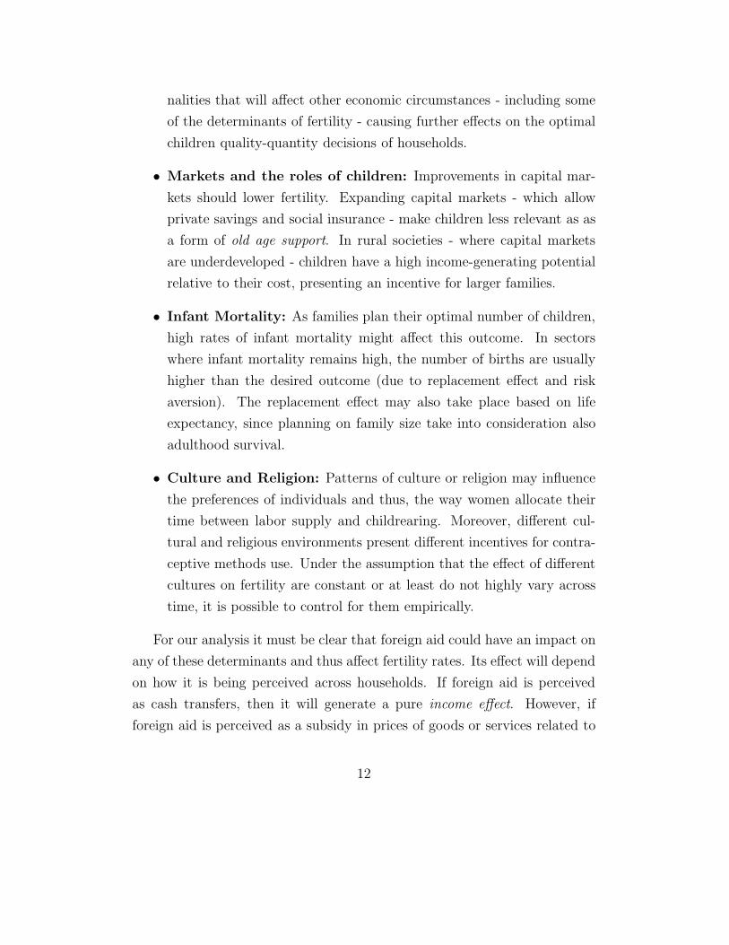
nalities that will affect other economic circumstances - including some

of the determinants of fertility - causing further effects on the optimal

children quality-quantity decisions of households.

• Markets and the roles of children: Improvements in capital mar-

kets should lower fertility. Expanding capital markets - which allow

private savings and social insurance - make children less relevant as as

a form of old age support. In rural societies - where capital markets

are underdeveloped - children have a high income-generating potential

relative to their cost, presenting an incentive for larger families.

• Infant Mortality: As families plan their optimal number of children,

high rates of infant mortality might affect this outcome. In sectors

where infant mortality remains high, the number of births are usually

higher than the desired outcome (due to replacement effect and risk

aversion). The replacement effect may also take place based on life

expectancy, since planning on family size take into consideration also

adulthood survival.

• Culture and Religion: Patterns of culture or religion may influence

the preferences of individuals and thus, the way women allocate their

time between labor supply and childrearing. Moreover, different cul-

tural and religious environments present different incentives for contra-

ceptive methods use. Under the assumption that the effect of different

cultures on fertility are constant or at least do not highly vary across

time, it is possible to control for them empirically.

For our analysis it must be clear that foreign aid could have an impact on

any of these determinants and thus affect fertility rates. Its effect will depend

on how it is being perceived across households. If foreign aid is perceived

as cash transfers, then it will generate a pure income effect. However, if

foreign aid is perceived as a subsidy in prices of goods or services related to

12

children, it sill generate both mechanisms (substitution and income effects),

and the final outcome it is very hard to predict. Moreover, goods or services

(such as schooling, food, health and others) are not exclusively related only

to quantity or to quality of children, but to both simultaneously, what makes

this prediction even harder. It is to be noticed that at the macro-empirical

level it is very difficult to identify what are the exact determinants of fertility

that are being affected by foreign aid. However, in this paper I give some

insights about this.7

In our empirical specification I carefully choose parameters which measure

directly or are proxy for most of these determinants. On one side, when us-

ing ordinary least squares, being able to do this represents a clear advantage,

since this will reduce the risk of omitted variable bias when adding foreign

aid to the regression. However, on the other side, every time the specifica-

tion is controlling for the determinants of fertility, it will be impossible to

estimate the overall effect of aid on fertility rates (including it effects on the

determinants themselves). Instead the estimate will represent the marginal

effect of foreign aid either directly on fertility or through a number of other

variables which are unobservable or not accounted for. It is to notice that

the risk of endogeneity is present only whenever any of the determinants of

fertility (both observables and unobservables) for which we do not control

for, presents some partial correlation with foreign aid.

2.2 About Foreign Aid and its determinants

Foreign aid as we know it today is a post World War II phenomenon. It is

not clear yet what are the main drivers of aid allocation. A Policy Research

Report of the World Bank explains foreign aid as follows (World Bank, 1998):

7Also notice that foreign aid may have externalities which might affect fertility throughother ways than just pure income or substitution effects, such as developing credit marketsor generating changes in institutions or fundamentals of the economy. In this paper Imean to estimate the overall effect of foreign aid on fertility which also includes theseexternalities.

13

“From the start, it had twin objectives, potentially in conflict.

The first objective was to promote long-term growth and poverty

reduction in developing countries; the underlying motivation of

donors was a combination of altruism and a more self-interested

concern that, in the long term, their economic and political se-

curity would benefit if poor countries were growing. The second

objective was to promote the short-term political and strategic in-

terests of donors. Aid went to regimes that were political allies

of major Western powers. Thus the strategic and developmental

objectives were potentially, but not necessarily, at odds.”

Many economist studied through cross country regressions the allocation

of foreign aid among recipients. All of them reached similar conclusions.

Foreign aid is not always allocated based on economic development goals.

Maizels and Nissanke (1984) found that bilateral aid flows fit best a model

in which aid serves donors interest, whereas a second model, in which aid

flows are meant to compensate for shortfalls in domestic resources fit multi-

lateral aid distribution. Boone (1996) finds that “(...)political factors largely

determine aid flows(...)” by finding significant estimators of political al-

liances dummies in his OLS and Fixed Effects regressions of foreign aid on

a number of other variables. Alesina and Dollar (2000) present a study in

which they found evidence that ”(...)factors such as colonial past and voting

patterns in the United Nations explain more of the distribution of aid than

the political institutions or economic policy of recipients.” These studies use

this fact as an explanation for the ineffectiveness of foreign aid (Alesina and

Dollar, 2000). On the other hand, GDP per capita still appears as one of

the strongest explanatory variables of foreign aid (Alesina and Dollar, 2000;

Boone 1996). However, there is no evidence that demographic variables such

as infant mortality and life expectancy measures have any explanation power

at all in foreign aid allocations (Boone, 1996).

14

Foreign aid from OECD countries increased significantly during the seven-

ties and eighties (see figure 1). Private aid flows have also started to increase

relative to official aid assistance. In the seventies and eighties, official aid

(bilateral and multilateral sources) represented about half of total aid flows.

As for 1996, official aid represents only a quarter of the total aid flows (World

Bank, 1998).

020

4060

80B

illio

ns o

f 200

0 P

PP

US

dol

lars

1960 1970 1980 1990 2000year

Europe Latin AmericaMiddle East East AsiaSub−Saharan Africa South Asia

Source: WDI 2005 and WDI 2007

Figure 1: Total ODA and Official Aid by World Region 1960-2000 (in Billionsof 2000 PPP US dollars)

However, following the review in the previous chapter, it is widely recog-

nized that foreign aid has barely proved itself as the solution to development

problems. As the World Bank report (1998) explains:

“Sadly, experience has long since undermined the rosy optimism

of aid financed, government led, accumulationist, strategies for

15

development. Suppose that development aid only financed invest-

ment and investment really played the crucial role projected by

early models. In that case, aid to Zambia should have financed

rapid growth that would have pushed per capita income above

$20,000, while in reality per capita income stagnated at around

$600.”

Some explanations for these failures are corruption or bad policies (Burn-

side and Dollar, 2000). Yet, in spite of the failure of foreign aid, it remains

as one of the primary solutions to economic stagnation and poverty across

developing countries (World Bank, 1998). Therefore, the debate on its direct

and indirect effects on other economic outputs, along with the way it should

be distributed, it is a highly relevant debate for economists and policy makers

nowadays.

3 Data Sources and Empirical Model

The main goal of this paper is to determine if foreign aid has any direct and

causal effect on fertility rates at macro levels. To do this, we estimate the

fertility equation with foreign aid being one of the covariates. The model to

estimate is:

fertit = β0 + aiditβa + yitβ+zitβ′z + σi + γt + δrt + εit (1)

Where i indexes countries, and t indexes time and r regions. fertit is

the fertility rate per woman, aidit is aid flows relative to GDP, yit represents

the logarithm of per capita GDP, zit is a Kx1 vector of exogenous variables

that affect fertility and might be correlated with aid, σi and γt correspond

to country specific fixed effects and time fixed-effects respectively, δrt is a

vector of regional linear time trends, and εit is a mean zero scalar.

Our variable of interest is βa, which measures (assuming strict exogeneity)

16

the marginal effect of one percentage point of aid as a share of the GDP on

the fertility rate per woman.

σi captures all the country fixed effects (such as colonial history or ge-

ographic conditions) affecting fertility which also might be correlated with

aid flows. Changes in the average level of fertility rates across time will be

absorbed by γt, the period fixed effects common to all countries. This in fact

will capture part of the common decline of the fertility rates across time. δrt

will control linearly for specific regional shocks on fertility across time.

The vector zit includes a number of exogenous variables which control for

most of the determinants of fertility reviewed in the previous chapter, such

as: infant mortality below one and five years, life expectancy at birth, share

of female workers in the labor force, rate of rural population and schooling

variables both across the female and male population.

The data was compiled mainly from the World Bank Development Indica-

tors (World Bank, 2005; World Bank, 2007), which includes data on foreign

aid, fertility rates and other macroeconomic variables used for the analysis

from 1960 to 2004, which will be the sample period. Consistent with the

literature, we constructed the main independent variable of interest by di-

viding Official Development Assistance (ODA) and Official Aid in current US

dollars by the GDP per capita in current US dollars, resulting in the share

of net ODA and Official Aid in the gross domestic product of each country

per year.8 ODA consists of net disbursements grants plus concessional loans

that have at least a 25 percent grant component (World Bank, 1998) to pro-

mote economic development and welfare in recipient economies. However, in

practice, ODA is virtually all grants (Boone, 1996). Official Aid refers to aid

flows from official donors to the transition economies of Eastern Europe and

the former Soviet Union and to certain advanced developing countries and

territories as determined by DAC. Both types of aid can be divided into bilat-

8Negative numbers of this measure indicate that the country was a net donor in thatspecific period.

17

eral and multilateral components. The former is assistance administrated by

agencies of the donor governments, while the latter is aid administrated by

international agencies such as the United Nations Development Programme

or the World Bank (World Bank, 1998). we use the ODA and Official Aid

share of the GDP variable without distinction of grants, loans, bilateral or

multilateral. If the variances across all these types of aid are similar, the

results will be robust to any subset of aid. Furthermore, the World Bank

report (1998) states regarding distinction between loans and grants: “The

macroeconomic effects of aid are the same regardless of which measure of aid

is used”. we restrict the dataset to countries which were never net donors of

ODA and Official Aid during the sample period (1960-2004).9

The dependent variable - total fertility rate per woman - is defined as the

number of children that would be born to a woman if she were to live to the

end of her childbearing years and bear children in accordance with prevailing

age-specific fertility rates. Fertility rates are documented in WDI on a yearly

basis for a partial set of countries, but it is included for most countries every

five years, starting in 1962 through 2002. Due the lack of availability of

fertility rates on a yearly basis, we averaged the variables in the dataset to

nine five-years periods starting from 1960-1964 through 2000-2004.

yit is measured making use of the Real GDP per capita (in 2000 US dollars

constant prices, Laspeyres) from the Penn World Tables 6.2 (Heston, Sum-

mer and Aten, 2006) . Additional macroeconomic variables include measures

on average schooling for women and men above age 25 per country and time

period as measured by Barro and Lee (2000). Since the number of obser-

vations for which the educational attainment variables are available is much

smaller than the base sample size, these covariates are inserted sequentially

in the regressions. In the rest of the paper, we refer to the sample which

includes the schooling variables as the reduced sample. The source of all the

other variables in the vector zit corresponds to the WDI.

9The results are robust to the inclusion of net donors (see Table A4 in the Appendix).

18

Finally, the data is merged with dataset on natural disasters from the

Emergency Events Dataset website. On a later chapter, this data will be

used to instrument foreign aid and thus establishing the causal effect of aid

on fertility rates.

The base panel data set consists of 96 countries across 9 five-years periods,

from 1960-1964 to 2000-2004. The countries in the sample respond to two

conditions: (1) they were always foreign aid net receivers during the sample

period (as measured by ODA and Official Aid) and (2) their population was

at least a million people during at least one period of time over the whole

sample period. The use of only “large countries” in the analysis is to avoid

an upward bias of the effect of the share of ODA in the GDP on fertility

rates. The small countries dropped from the sample tend to have a much

higher mean of ODA and Official Aid as a share of GDP (16.73% in constrast

to 7.79% of the rest of the sample), being many of them developing countries

with high fertility rates. In any case, the main results stays unaffected by

their inclusion.10 The list of all countries in the sample is covered in Table

A1. The number of observations, and therefore the number of countries, used

in the regressions will depend on the control variables availability.

Summary statistics for the key variables are presented in Table 1. The

mean fertility rate is 5.28 children per woman for the base dataset, being half

of the observations with a fertility rate below 5.84. ODA and Official Aid

represents in average 7.5% of the GDP, with half of the observations having

less than 4.45% of the GDP. In a typical low-income country, foreign aid is

the main external source of finance, averaging between 7 and 8 percent of

the GNP (World Bank, 1998).

The real gross domestic product, in 2000 US dollars, averages 3038 dollars

per capita in the sample. The maximum value of the real GDP is 21,348.12

real 2000 US dollars, which corresponds to Israel in the 2000-2004 period. 11

10See Table A5 in the Appendix.11Consistently with the literature, robustness test were made excluding Israel and Egypt

from the sample, which present an irregular aid trend since the Camp David accords. Their

19

However, 90% of the countries in the sample have a real GDP lesser than 7000

US dollars (in constant US dollars 2000 prices). As can be inferred from the

statistics, most of the countries in the sample are developing countries. Table

A2 provides some country-specific information about the main variables of

focus.

3.1 Explaining Fertility

The dependent variable of the study is the fertility rate per women. In order

to understand the behavior of the determinants of fertility using the sample

data, we estimate the model:

fertit = β0 + yitβ+zitβ′z + σi + γt + δrt + υit (2)

Table 2 presents results of the estimation of model (2) being zit the deter-

minants of fertility. In the first 8 columns, the data used is not limited to the

base dataset of the analysis, and they include also high income countries for

which data of the WDI is available.12 The variables in columns 1 through 5

can explain at most 84% of the variance in fertility rates accross countries and

time. Adding regional dummies and a regional linear time trend in the next

two columns explain slightly more, but when adding country specific fixed

effects the explanatory power of all the covariates together raises to 95%.

The signs of all the covariates are consistent with the theory and previous

literature (Birdsall, 1988; Behrman, Duryea and Szekely, 1999).

When reducing the sample to both the base and reduced dataset of this

analysis (columns 9 and 10 respectively), the explanatory power stays above

93%. Therefore, by making use of all the explanatory variables (including

the country specific fixed-effects, time dummies and the regional linear time

trend) it is possible to explain most of the cross-country change in the fertility

exclusion does not affect the results (see Table A5 in the Appendix).12All the data is collapsed to five-years periods as the base dataset.

20

rates in the period of time covered by the sample.

We can deduce from these results that the determinants of fertility that

were reviewed in the previous section account for most of the variation of

fertility rates in our sample.

4 The effect of Foreign Aid on Fertility

4.1 OLS Estimates

Table 3 presents OLS estimates for model (1) omitting the σi component.

There are two main disadvantages to this method. First, country specific

characteristics (i.e. colonial past, location, climate conditions and other fixed

attributes) are not controlled for, and the error term becomes σi +εit. Hence,

the estimates of βa possibly present omitted variable bias since aid alloca-

tions are associated with σi: colonial past and long term alliances between

countries (Boone, 1996; Alesina and Dollar, 2000). Second, the results of

βa will represent the effect of foreign aid either directly on fertility rates or

through unobservables or unmeasured covariates which are not present in

the regressions. Hence, through OLS it is not possible to study the overall

effect of aid on fertility, because omitting variables in the regressions would

possibly result in biased estimators for βa. This is because the allocation of

aid might be correlated with health and schooling outcomes like the ones we

are controlling for.

The first column presents a simple and naive specification which results in

a positive and significant estimate for βa. Column 2 to 4 include sequentially

most of the determinants of fertility (but schooling). All these regressions

present positive estimates for βa, and some of them significant, ranging from

0.010 to 0.014. However, the estimates could be biased since there is no

control for σi. Column 5 includes control for absolute latitude and regional

fixed effects, trying to reduce some of the bias caused by omitting σi. In

this specification the variable of interest losses significance. The last column

21

repeat the previous specification but including the schooling variables, and

thus using only the reduced sample. This last column shows positive and

significant estimates for βa standing at 0.024 additional children per woman

for every percentage point increase of aid as a share of the GDP. However,

the use of the reduced sample arises the possibility that the results suffer of

selection sample bias. This is covered in the next sub-section.

These estimates are unbiased only under the assumption that, once con-

trolling for all the determinants of fertility (not including country specific

fixed effects), foreign aid is not correlated with the error term. Being this as-

sumption hardly reliable, we turn to make the analysis through fixed effects

estimation.

4.2 Fixed Effects Estimates

Table 4 presents the results of estimating model (1) using the Fixed Effects

estimator. By using this method we overcome endogeneity problems that

arises due to the correlation between country fixed specific characteristics

and foreign aid allocations. The estimates of βa are unbiased only under the

strict exogeneity assumption:

E(εit|aidit, yit, zit, σi, γt, δrt) = 0 (3)

However, still it is not possible to study through this method the overall

effect of aid on foreign aid, since omitting variables could produce bias on the

estimates of βa. Hence, the results of this section may represent the effect

of aid on fertility through other variables which are not accounted for, such

as non-wage cash transfers to families - representing a pure income effect, or

subsidies in the cost of food, which in case of poor families might increase

their decision on the optimal number of children. Another disadvantage of

this method is that, even though it controls for countries’ fixed effects, the

strict exogeneity assumption does not necessarily hold.

22

The first column presents a naive specification controlling only for yit,

thus obtaining biased estimates for βa. Column 2 through 4 controls pro-

gressively for all the variables available for the base dataset of 95 countries.13

Based in the estimates in all these columns, there is no evidence that the

effect of foreign aid on fertility rates is statistically different from zero. How-

ever, columns 5 shows a positive and significant estimate for βa, and this

happens when controlling for the schooling variables. As explained before,

the availability of the schooling variables is restricted to observations for only

the 50 countries of the reduced dataset.14 From here arises the possibility

that the estimate of the variable of interest in column 5 is driven by sample

selection bias. Column 6 shows an informative regression identical as column

4 but only on the reduced sample. It can be seen that the estimate for βa,

although not statistically different from zero, is very similar in magnitude

than the one of column 5, making a strong case that the reduced sample

generates a sample selection bias.

It is of our interest to understand if the main variables of interest are cor-

related with the probability of being in the sample or not. The distributions

of fertility and foreign aid variables across both datasets are strongly similar.

In the reduced dataset ODA and Official Aid (as a share of GDP) averages

7.04 percentage, with a standard deviation of 7.57, and fertility averages 5.56

with a standard deviation of 1.52, which are close to the statistics of the base

dataset presented in Table 1. Figure 2 presents a scatter of the foreign aid

values against the fertility rates both in the base and reduced dataset. It

can be seen that there is virtually no difference in the distribution of these

variables across both datasets. Figure 3 also presents the Kernel Density

lines for fertility rates and foreign aid flows in both the base and reduced

samples. The lines are almost superimposed one against the other, meaning

13Libya was dropped from the sample since it consists of a single point of time observa-tion, lacking of within variation.

14Burundi and Mauritania were dropped out of the sample since each country had asingle point of time observation in the reduced dataset

23

that the distribution of both datasets are highly alike.

24

68

10F

ertil

ity R

ate,

tota

l birt

hs p

er w

oman

0 20 40 60Foreign Aid (share of GDP)

Base Dataset Reduced Dataset

Figure 2: Scatter of ODA and Official Aid (as a share of GDP) Vs. FertilityRates per woman in both the base and the reduced sample

A more analytical approach is presented in Table 5. This table presents

the results of a probit model which intends to measure the probability of

being in the reduced sample. The regression included as regressors aidit,

fertit, yit and Zit. As can be seen from the results, when controlling for

all the variables, neither specific levels of fertility rates or aid flows explain

the probability of being in the sample. However, in order to assure that

the results of column 5 in table 4 lack of sample selection bias, one must

assume that the error term of the selection equation is uncorrelated with

εit. Column 6 in table 4 presents a case against this assumption due to the

similarity in magnitude of βa estimate with column 5. Hence, the reliability

of this assumption cannot be fully proved. Any presence of unobservables

which are correlated both with fertility and foreign aid (violating the strict

exogeneity assumption), or correlated with the probability of being in the

reduced sample (generating sample selection bias) can be causing distortion

24

0.1

.2.3

Ker

nel D

ensi

ty (

Fer

tility

Rat

e)

2 4 6 8 10

Base Reduced

0.0

2.0

4.0

6.0

8.1

Ker

nel D

ensi

ty (

For

eign

Aid

, sha

re o

f GD

P)

0 20 40 60

Base Reduced

Figure 3: Kernel Densities of ODA and Official Aid (as a share of GDP) andFertility Rates per woman in both the base and reduced dataset

on the results. This possibility is covered in the next section.

5 Establishing a causal effect: how many for-

eign aid dollars produce another child?

Preceding sections demonstrate a positive correlation between foreign aid and

fertility. Yet, it cannot be proved that this correlation actually represents a

causal effect of foreign aid on fertility rates. In this section we instrument for

foreign aid making use of natural disasters data on neighboring countries.

The number of natural disasters in neighboring countries of X is a valid

instrument if (1) they have a direct impact on foreign aid flows to country

X and (2) they are not correlated with the children production of country

X (but only and exclusively though the effect of aid allocations). There

are several reasons why this claim is consistent. First, natural disasters

25

are exogenous. Moreover, the relevant claim is that natural disasters in

country Y are exogenous to the fertility decisions of households in country

X. However, given the case that natural disasters in neighboring countries

have any effect in the fertility rates, the impact will be translated in terms

of the determinants of fertility, or directly through regional shocks in the

specific point of time of the disaster (i.e. refugees, migration, etc). Hence,

we include in 2SLS sequentially the determinants of fertility. The robustness

of the results hints that this is not the case.

The new model to estimate becomes:

fertit = β0 + ˆaiditβa + yitβ+zitβ′z + σi + γt + δrt + εit (4)

In which ˆaidit is the first stage regression fitted values of foreign aid,

and the rest of the specification is identical to model (1). The instrumental

variable can be properly defined as the number of natural disasters that

occurred in neighboring countries (that belong to the same region)15 during

the same period of time. The data was acquired from the Emergency Events

Dataset, and summed up to five-years periods to suit the panel data sample.

we restricted the disasters dataset only to data on earthquakes, floods, wind

storms, volcanoes and slides, under the assumption that these disaster types

are exogenous and of sudden natural occurrence.16

There are two main advantages of instrumenting for foreign aid. First,

that the estimates of βa will be unbiased. Second, the exogeneity of foreign

aid flows in the estimation will allow us to omit certain determinants of

fertility without the risk of omitted variable bias, and thus being able to

study the overall effect of foreign aid. If foreign aid is having also effects on

15Regions as defined by the World Bank: North America, Latin America and theCaribbean, Europe, Sub-Saharan Africa, East Asia and the Pacific, Middle East andNorth Africa, and South Asia.

16Other disaster types in the dataset, such as epidemics, extreme temperature anddroughts, are more predictable and therefore could have an effect not only through changesin aid flows but directly on the fertility production function of the countries non-affectedby the disasters.

26

schooling or health outcomes and consequently any effect on fertility rates,

our estimate will capture this when omitting the relevant covariates from the

regression.

Table 6 presents summary statistics of the natural disasters merged in

the sample. There are 2993 natural disasters reported distributed over 3170

country-year observations of the base dataset.17 On average, there are 6.36

natural disasters in every country every year. The average number of killed

and injured people per disaster is around 400 and 800 respectively. However,

90 percent of the disasters had less than 226 killed victims and less than

200 injured, which in terms of total population can be classified as small

impact disasters. This suggests that most of the disasters are not expected

to have direct impact on the fertility rate of localities outside the limits of

the country in which they occurred. We do expect however changes in aid

allocations in response to natural disasters.

Government spending on humanitarian emergencies is dominated by the

United States (Cohen and Werker, 2007). The Congressional Budget Justi-

fication of the American USAID agency, an independent federal government

agency that manages foreign aid policy, specifies that foreign aid is budgeted

in advance by geographical regions (USAID, 2008). Each budget justification

has an specific clause for humanitarian assistance, which in 2007 was above

USD 10 billions. However, because of the unanticipated nature of many dis-

asters, humanitarian aid budget allocations often increase throughout the

year as demands arise (Nowels and Tarnoff, 2004). Hence, in the presence

of unexpected natural disasters, some countries will suffer from a decrease

in their aid allocations due to the need of give immediate assistance to the

affected countries. In general, it is possible for governments to adjust their

aid on short notice (Kuziemko and Werker, 2006).

This claim is consistent with the dataset: a larger number of natural

17The table is presented on terms of single years. Table A3 presents a breakdown of thedisasters per country over the 1960-2004 period that are part of the base dataset

27

disasters in neighboring countries of country X lowers significantly the foreign

aid flows to the latter. Evidence of this is the first stage regressions, which

are showed in Table 7A. For the different specifications, it can be seen that an

additional natural disaster in the neighbor countries will decrease the share

of foreign aid of the GDP in a range of 0.044 to 0.051 percentage points,

being this estimate statistically significant in all specifications with p-values

below 0.01. It can be seen that other variables are consistent with intuition

on the allocation of aid.

At the country-level, a graphical representation of what happens is pre-

sented in figures 4 and 5. Figure 4 reveals data from Congo across time (from

the period 1960-64 to 2000-2004). The left panel describes the behavior of

both the number of natural disasters among Congo’s neighbors, and foreign

aid flows received by Congo, while the right panel presents a version of these

two variables “cleaned” from their perceptible time trends (in order to take

into account the relativeness of each period). It is easily noticeable that in

the presence of a large amount of natural disasters in the region (excluding

Congo), the foreign aid receipts for Congo drop substantially.

Figure 5 shows how Haiti’s foreign aid receipts behave similarly to Congo’s

in response to natural disasters in Latin America and the Caribbean region

(excluding Haiti). Again, the right panel is a “detrended” version of the left

panel. This behavior is consistent mostly among all countries in the sample.18

The exogeneity of natural disasters in neighbor countries and its remark-

able impact on foreign aid of each country makes this a plausible instrument

to estimate the effect of foreign aid on fertility.

Table 7B shows 2SLS results using the number of natural disasters in

neighbor countries as an IV. This time, the naive specification of controlling

only for GDP per capita in the first column result in a positive and significant

coefficient for the effect of foreign aid on fertility per woman, standing on

18Figures A1 and A2 in the appendix compiles the “detrended” version of these graphsfor all countries in the sample.

28

050

100

150

200

Nei

ghbo

rs’ D

isas

ters

010

2030

For

eign

Aid

0 2 4 6 8 10period

Aid Disasters

−50

050

100

Det

rend

ed N

eigh

bors

’ Dis

aste

rs

−10

−5

05

1015

Det

rend

ed F

orei

gn A

id

0 2 4 6 8 10period

Aid Disasters

Figure 4: ODA and Official Aid in Congo in response to natural disasters inits neighbors

0.045 additional child per woman for every percentage point increase of aid as

a share of GDP. This effect includes the overall effect of aid flows, also through

its effects on schooling, health and other outcomes that explain fertility.

Columns 2 and 3, which control for labor market and health measures, also

present similar estimates of foreign aid on fertility, which are both positive

and statistically significant. The fourth column presents a slight smaller -

but still robust - estimate for βa in magnitude, not statistically significant,

even though its p-value stands at 0.109. The last column includes schooling

variables, which drop the sample by slightly less than half, and the estimate

for βa is 0.054, statistically significant at the 5% level. The results show

that the OLS and FE estimates were downward biased. This is consistent

with the intuition. Any unobservable measure of “development”, such as

human capital accumulation, that for sure affects fertility decisions across

households, will be negatively correlated with aid flows.19

19Similar regressions like the ones in Table 7 were also made using total fertility rate

29

5010

015

020

025

0N

eigh

bors

’ Dis

aste

rs

24

68

1012

For

eign

Aid

0 2 4 6 8 10period

Aid Disasters

−10

0−

500

5010

0D

etre

nded

Nei

ghbo

rs’ D

isas

ters

−6

−4

−2

02

4D

etre

nded

For

eign

Aid

0 2 4 6 8 10period

Aid Disasters

Figure 5: ODA and Official Aid in Haiti in response to natural disasters inits neighbors

The table also reports the first stage F test. The values suggest that

the we are not in the presence of a weak instrument. The robustness of

the results across all the specifications suggest that βa is unbiased, and the

results are consistent with the hypothesis that foreign aid is having a causal

and positive effect on the fertility rates of the developing countries.

Furthermore, the robustness of the results give some insights about the

mechanism that is working behind this relationship. The effect of aid on

fertility stays robust in the presence of other determinants. This allow us to

infer two claims. First, aid flows is having virtually no effect on health, labor,

market development and schooling outcomes which can account for variations

of fertility and are present in the regressions. Second, consequently, aid flows

are increasing fertility through other variables which are not being controlled

one period ahead as the dependent variable, since the effects of aid might not be seenimmediatly. The results are robust to the ones presented in the paper, being slightlyhigher and more significant in almost most of the specifications.

30

for, such as cash transfer to families, subsidies in food costs, unobservable

variables related to culture or institutions and others. Therefore, aid is being

perceived as non wage extra income that is inducing a purely income effect,

or perceived as a subsidy in children costs (aside from the ones that are

being controlled for), causing that the increase in the quantity of children

is the dominating effect in the household utility maximization problem. At

the macro level it is not possible to identify exactly what is the main driver

of this causal relationship. However, an empirical analysis at the household

level could give a better explanation to this phenomenon. This, however, is

out of the range of this research.

The estimated effect averages 0.045 additional child per woman for every

percentage point increase of ODA and Official Aid receipts as a share of

the GDP. In other words, this means an additional child for about every 22

women. If we take Tanzania as an example, this marginal effect could be

translated to over 300 thousand children per one percentage point increase

in the share of foreign aid in the GDP of Tanzania, or above 1.5 million new

children for one standard deviation increase of the same parameter (based

on 2000-2004 average population).20 Figure 6 presents rough estimations of

one percentage point increase and one country-specific standard deviation

increase of foreign aid as a percentage of GDP for a selected sample of the

countries in the base dataset for the period 2000-2004. The numbers suggest

that the impact on population growth is non negligible, providing another

possible explanation to the lack of efficacy of foreign aid.

20This was computed using as the childbearing population the share of female populationaged 15-50 (assuming a uniform distribution of ages between the group aged 15-64).

31

0

1,000,000

2,000,000

3,000,000

4,000,000

5,000,000

Algeria

Bangla

desh

Bosnia

and

Her

zego

vina

Burun

di

Cambo

dia

Democ

ratic

Rep

ublic

of t

he C

ongo

Ethiop

ia

Ghana

Indo

nesia

Kenya

Mad

agas

car

Mala

wi

Nepal

Niger

Nigeria

Pakist

an

Rwanda

Sri La

nka

Sudan

Ugand

a

United

Rep

ublic

of T

anza

nia

Viet N

am

Zambia

Additional Children due to 1% increase in Aid/GDP

Additional Children due to one local s.d. increase in Aid/GDP

Figure 6: Estimated number of additional children due to an increase in aidflows, per country (based on 2000-2004 average population)

6 Exploring Further the Effectiveness of For-

eign Aid

Having found a proper instrumental variable for foreign aid, we can extend

this specification to study its effect on other dependent variables.

The robustness of the results in table 6 allow us to assume strict exo-

geneity of the first stage fitted values of foreign aid flows. Therefore, it is

reasonable to assume strict exogeneity of following empirical model:

outcomeit = β0 + ˆaiditβa + yitβ+σi + γt + δrt + rit (5)

32

Similarly to model (1), i indexes country, t indexes time and r indexes

region. outcomeit is a vector of economic variables of interest which foreign

aid intents to influence. ˆaidit is the instrumented version of the foreign aid

variable (using natural disasters in neighboring countries), yit is real GDP per

capita, σi is a vector of country fixed effects, γt is a vector of time common

effects, δrt represents a regional linear time trend and rit is a mean zero

residual term.

By making use of this simplistic specification, it is possible to estimate

consistently the marginal effect of foreign aid flows on other variables such

as labor market outcomes, health outcomes, investment or economic growth.

Table 8 presents results of 2SLS regressions which estimate the effect of for-

eign aid flows on seven economic outcomes. Regarding most of the variables,

there is no evidence that foreign aid flows have any effect of them. The share

of the total labor force in the population and the share of female workers in

the labor force is not being improved by aid flows. Likewise, infant mortality

is not being affected by foreign aid flows. However, regarding life expectancy,

which is a proxy variable for general health determinants of the population,

the results show a positive and significant coefficient for foreign aid as a share

of GDP. Regarding schooling outcomes, there is no evidence of improvement

measured by average years of schooling in the population. It can be noticed

that the sign of the estimate appears negative, being consistent with the

theoretical framework.21 Regarding economic growth variables, there is no

evidence that investment shares are positively affected by foreign aid flows.

Lastly, column 7 shows results when using real GDP growth per capita as the

dependent variable, finding no evidence that it is being affected by foreign

aid flows.

From this analysis can be inferred that foreign aid is not having impact in

labor markets or schooling outcomes of developing countries. Similarly, there

is no evidence that aid is having any impact on the determinants of growth

21In this case the relevant sample is the reduced sample.

33

or economic growth itself. Regarding health outcomes the results are not

clear. Aid appears to be effective in increasing the life expectancy in devel-

oping countries, but is having no effect on infant mortality whatsoever. The

allocation of aid flows to distribute medicines to combat the HIV epidemics

in Africa could give a proper explanation to this phenomenon.

7 Concluding Remarks

Even thought foreign aid flows as we know them today started immediately

after World War II, only during the last decade or two economists started

to estimate its impact and effectiveness. This paper opens a new path of re-

search on the study of foreign aid. Most of the research until now was limited

mostly to the effect of aid on economic growth, ignoring other determinants

of economic prosperity, such as fertility rates.

The primary question of this research was whether foreign aid can explain

partially the high fertility rates in developing countries. By making use

of natural disasters in neighboring countries as an instrumental variable to

foreign aid, we have found that aid have a positive and significant effect

on fertility rates across countries, and found no evidence that aid flows are

improving other economic outcomes, except life expectancy.

There are two important contributions in this research. First, the empir-

ical strategy of instrumenting for foreign aid makes allow us to establish a

causal relationship between foreign aid and fertility. Recent literature on for-

eign aid flows lacks of proper instrumental variables to overcome endogeneity

issues in their specifications. Therefore, the results presented in them, not

only are not robust,22 but are not reliable enough.

Second, the sole idea of examining the effect of foreign aid on the de-

terminants of growth, and not growth itself, can lead us to conclude that

aid policies should be aimed to generate the proper incentives so that it will

22Roodman, 2007

34

impact the determinants of growth on the right direction, and therefore, in

the long run, aid flows would contribute to economic growth.

An important point is that this paper does not suggest that aid flows

should be eliminated, but that the allocation of aid both across countries and

projects should be done carefully enough. This in order to avoid undesired

incentives and creating a “medicine that worsens the illness”.

The fact that aid flows in the last decade have decreased might be a

consequence of the recent global debate on the effectiveness of foreign aid.

This is not necessarily a bad signal. It might also hint of a process in which

development agencies are improving efficiency on their aid allocations, dis-

tributing less aid on more efficient projects. If this claim happens to be true,

then we should expect aid to be much more effective in the near future, and

see the developing world enjoying its fruits.

35

Tab

le1

-Sum

mar

ySta

tist

ics

NM

ean

SDM

inM

edia

nP

75P

90M

axO

DA

and

Offi

cial

Aid

(as

perc

enta

geof

GD

P)

608

7.51

8.91

0.00

14.

4510

.04

18.3

254

.91

Fert

ility

rate

,tot

al(b

irth

spe

rw

oman

)60

85.

281.

871.

155.

846.

707.

2010

.13

Rea

lper

capi

taG

DP

(Con

stan

tP

rice

s:Las

pery

res)

608

3038

.05

3129

.22

294.

2219

41.6

037

48.3

269

68.9

221

348.

12M

orta

lity

rate

,inf

ant

(per

1,00

0liv

ebi

rths

)59

292

.86

49.0

44.

0094

.80

127.

0015

7.00

255.

00M

orta

lity

rate

,und

er-5

(per

1,00

0)59

214

5.20

85.9

14.

5014

4.00

204.

5025

5.00

450.

00R

ural

popu

lation

(%of

tota

lpop

ulat

ion)

608

65.7

818

.93

8.52

67.6

881

.35

88.5

897

.92

Lab

orfo

rce,

fem

ale

(%of

tota

lla

bor

forc

e)60

838

.71

9.55

6.21

41.0

846

.03

48.9

153

.16

Life

expe

ctan

cyat

birt

h,to

tal(

year

s)60

854

.75

10.8

134

.71

52.7

064

.63

70.6

679

.03

Ave

rage

scho

olin

gye

ars

inth

eto

talpo

pula

tion

(>25

)39

42.

831.

980.

042.

343.

955.

489.

90A

vera

gesc

hool

ing

year

sin

the

fem

ale

popu

lation

(>25

)39

32.

282.

050.

001.

543.

325.

169.

74A

vera

gesc

hool

ing

year

sin

the

mal

epo

pula

tion

(>25

)39

33.

412.

000.

083.

104.

595.

9710

.09

36

Table

2-

The

determ

inants

ofFertility

(1)

(2)

(3)

(4)

(5)

(6)

(7)

(8)

(9)

(10)

Log

RealPer

Capit

aG

DP

-1.2

72

***

-0.1

12

**

-0.2

05

***

-0.1

44

***

-0.2

67

***

-0.1

74

**

-0.2

69

***

-0.0

50

-0.0

966

-0.0

84

(Const

ant

Pri

ces:

Lasp

ery

res)

(0.0

36)

(0.0

51)

(0.0

70)

(0.0

51)

(0.0

73)

(0.0

75)

(0.0

80)

(0.1

10)

(0.1

10)

(0.1

10)

Labor

forc

e,fe

male

-0.0

62

***

-0.0

34

***

-0.0

59

***

-0.0

28

***

-0.0

13

***

-0.0

11

**

-0.0

10

0.0

0872

-0.0

03

(%ofto

talla

bor

forc

e)

(0.0

03)

(0.0

04)

(0.0

03)

(0.0

04)

(0.0

05)

(0.0

05)

(0.0

08)

(0.0

11)

(0.0

10)

Mort

ality

rate

,in

fant

0.0

01

-0.0

03

0.0

01

-0.0

04

-0.0

01

-0.0

01

0.0

07

0.0

0102

-0.0

05

(per

1,0

00

live

bir

ths)

(0.0

04)

(0.0

04)

(0.0

03)

(0.0

04)

(0.0

04)

(0.0

04)

(0.0

05)

(0.0

04)

(0.0

04)

Mort

ality

rate

,under-

50.0

03

0.0

06

**

0.0

03

0.0

05

**

0.0

04

0.0

03

0.0

03

0.0

0162

0.0

07

***

(per

1,0

00)

(0.0

02)

(0.0

03)

(0.0

02)

(0.0

03)

(0.0

03)

(0.0

03)

(0.0

03)

(0.0

02)

(0.0

03)

Life

expecta

ncy

at

bir

th,to

tal

-0.0

99

***

-0.0

73

***

-0.1

02

***

-0.0

78

***

-0.0

63

***

-0.0

59

***

0.0

162

0.0

21

**

0.0

07

(years

)(0

.009)

(0.0

11)

(0.0

08)

(0.0

10)

(0.0

11)

(0.0

11)

(0.0

12)

(0.0

10)

(0.0

11)

Rura

lpopula

tion

0.0

12

***

-0.0

01

0.0

10

***

-0.0

03

0.0

03

0.0

02

0.0

22

***

0.0

255

***

0.0

16

**

(%ofto

talpopula

tion)

(0.0

02)

(0.0

02)

(0.0

02)

(0.0

02)

(0.0

02)

(0.0

02)

(0.0

06)

(0.0

07)

(0.0

07)

Avera

ge

schooling,fe

male

-0.0

584

-0.0

64

*-0

.142

***

-0.1

24

***

-0.2

21

***

-0.2

72

***

(years

,popula

tion

age

>25)

(0.0

40)

(0.0

38)

(0.0

41)

(0.0

41)

(0.0

53)

(0.0

70)

Avera

ge

schooling,m

ale

-0.1

13

***

-0.0

95

***

0.0

24

-0.0

02

-0.0

33

-0.1

37

*(y

ears

,popula

tion

age

>25)

(0.0

37)

(0.0

35)

(0.0

37)

(0.0

37)

(0.0

63)

(0.0

76)

Sub

Sahara

nA

fric

a0.2

37

0.6

30

**

(0.2

10)

(0.2

70)

South

Asi

a(-

0.4

90)**

(0.0

00)

(0.2

10)

(0.0

00)

Nort

hA

meri

ca

0.0

00

-0.2

74

(0.0

00)

(0.4

10)

Mid

dle

East

and

Nort

hA

fric

a0.6

61

***

1.8

29

***

(0.2

00)

(0.3

50)

Lati

nA

meri

ca

and

the

Cari

bbean

0.2

64

0.9

99

***

(0.1

60)

(0.2

60)

Euro

pe

-0.5

76

***

-0.8

29

***

(0.1

50)

(0.2

90)

East

Asi

aand

the

Pacifi

c-0

.251

0.0

72

(0.1

70)

(0.3

30)

Const

ant

14.9

***

12.6

3***

12.2

6***

13.0

90

***

13.0

00

***

10.0

80

***

10.3

70

***

3.7

88

***

3.4

99

**

5.4

67

***

(0.2

90)

(0.7

00)

(0.8

10)

(0.6

60)

(0.7

80)

(0.9

40)

(0.9

80)

(1.3

90)

(1.3

80)

(1.3

90)

Tim

eFix

ed

Effects

No

No

No

Yes

Yes

Yes

Yes

Yes

Yes

Yes

Countr

yFix

ed

Effects

No

No

No

No

No

No

No

Yes

Yes

Yes

Lin

ear

Regio

nT

ime

Tre

nd

No

No

No

No

No

No

Yes

Yes

Yes

Yes

Rese

arc

hSam

ple

Only

No

No

No

No

No

No

No

No

Yes

Yes

Obse

rvati

ons

1,3

37

1,1

70

800

1,1

70

800

800

800

800

592

386

Adju

sted

R-s

quare

d0.5

10.8

10.8

30.8

20.8

40.8

60.8

70.9

50.9

50.9

3Legend:

***

p<

0.0

1,**

p<

0.0

5,*

p<

0.1

Note

s:R

obust

standard

err

ors

inpare

nth

ese

s,clu

stere

dby

countr

y.

37

Tab

le3

-O

rdin

ary

Lea

stSquar

esR

esult

s(1

)(2

)(3

)(4

)(5

)(6

)O

DA

and

Offi

cial

Aid

0.01

5*

0.01

4*

0.01

00.

012

*0.

009

0.02

4**

(%G

DP

)(0

.008

)(0

.008

)(0

.006

)(0

.006

)(0

.006

)(0

.011

)Log

Rea

lPer

Cap

ita

GD

P-0

.456

**-0

.544

***

-0.1

72-0

.004

-0.0

300.

151

(Con

stan

tP

rice

s:Las

pery

res)

(0.1

80)

(0.1

60)

(0.1

50)

(0.1

50)

(0.1

50)

(0.2

00)

Lab

orfo

rce,

fem

ale

-0.0

24*

-0.0

26**

-0.0

32**

*-0

.028

**-0

.004

(%of

tota

lla

bor

forc

e)(0

.012

)(0

.011

)(0

.011

)(0

.012

)(0

.014

)M

orta

lity

rate

,inf

ant

0.00

50.

003

0.00

7-0

.002

(per

1,00

0liv

ebi

rths

)(0

.006

)(0

.007

)(0

.006

)(0

.007

)M

orta

lity

rate

,und

er-5

0.00

10.

003

-0.0

000.

004

(per

1,00

0)(0

.004

)(0

.004

)(0

.004

)(0

.005

)Life

expe

ctan

cyat

birt

h,to

tal

-0.0

48**

-0.0

34*

-0.0

39**

-0.0

20(y

ears

)(0

.019

)(0

.019

)(0

.019

)(0

.022

)R

ural

popu

lation

0.01

9**

*0.

017

***

0.00

5(%

ofto

talpo

pula

tion

)(0

.007

)(0

.006

)(0

.010

)A

vera

gesc

hool

ing

for

fem

ale

-0.2

20(y

ears

,pop

ulat

ion

age

>25

)(0

.130

)A

vera

gesc

hool

ing

for

mal

e0.

001

(yea

rs,p

opul

atio

nag

e>

25)

(0.1

20)

Abs

olut

eLat

itud

e-0

.017

-0.0

08(0

.011

)(0

.014

)Su

bSa

hara

nA

fric

a0.

771

1.04

7(0

.530

)(0

.630

)So

uth

Asi

a0.

184

0.71

6(0

.540

)(0

.630

)M

iddl

eE

ast

and

Nor

thA

fric

a1.

642

***

1.56

5**

(0.4

90)

(0.6

20)

Lat

inA

mer

ica

and

the

Car

ibbe

an0.

923

*1.

452

**(0

.550

)(0

.670

)E

ast

Asi

aan

dth

ePac

ific

0.16

30.

595

(0.8

30)

(0.8

70)

Con

stan

t10

.230

***

11.7

00**

*10

.320

***

7.08

1**

*7.

046

***

5.09

1(1

.290

)(1

.220

)(1

.460

)(1

.830

)(1

.860

)(3

.120

)

Obs

erva

tion

s60

860

859

259

259

238

6A

djus

ted

R-s

quar

ed0.

790.

800.

840.

850.

860.

79Leg

end:

***

p<

0.0

1,**

p<

0.0

5,*

p<

0.1

Note

s:R

obust

standard

erro

rsin

pare

nth

eses

,cl

ust

ered

by

countr

y.A

llth

eco

lum

ns

contr

olfo

rti

me

fixed

effec

tsand

spec

ific

regio

nti

me

tren

d.

38

Tab

le4

-Fix

edEffec

tsEst

imat

ion

Res

ult

s(1

)(2

)(3

)(4

)(5

)(6

)O

DA

and

Offi

cial

Aid

0.00

60.

006

0.00

80.

005

0.01

3*

0.01

2(%

GD

P)

(0.0

05)

(0.0

05)

(0.0

06)

(0.0

06)

(0.0

07)

(0.0

08)

Log

Rea

lPer

Cap

ita

GD

P-0

.204

-0.2

05-0

.072

-0.0

470.

061

-0.0

73(C

onst

ant

Pri

ces:

Las

pery

res)

(0.1

80)

(0.1

80)

(0.1

90)

(0.1

90)

(0.2

10)

(0.2

20)

Lab

orfo

rce,

fem

ale

0.02

10.

012

0.00

9-0

.003

0.00

0(%

ofto

talla

bor

forc

e)(0

.022

)(0

.018

)(0

.017

)(0

.016

)(0

.019

)M

orta

lity

rate

,in

fant

0.00

10.

001

-0.0

05-0

.002

(per

1,00

0liv

ebi

rths

)(0

.006

)(0

.006

)(0

.005

)(0

.006

)M

orta

lity

rate

,un

der-

50.

002

0.00

20.

008

**0.

004

(per

1,00

0)(0

.004

)(0

.004

)(0

.003

)(0

.003

)Life

expe

ctan

cyat

birt

h,to

tal

0.01

70.

022

0.01

00.

018

(yea

rs)

(0.0

15)

(0.0

13)

(0.0

14)

(0.0

16)

Rur

alpo

pula

tion

0.02

5**

*0.

015

0.02

9**

(%of

tota

lpo

pula

tion

)(0

.008

)(0

.011

)(0

.012

)A

vera

gesc

hool

ing

for

fem

ale

-0.2

89**

*(y

ears

,po

pula

tion

age

>25

)(0

.098

)A

vera

gesc

hool

ing

for

mal

e-0

.121

(yea

rs,po

pula

tion

age

>25

)(0

.120

)C

onst

ant

8.07

0**

*7.

300

***

5.19

5**

3.10

74.

195

**3.

761

(1.2

90)

(1.5

70)

(2.0

80)

(2.1

40)

(1.9

80)

(2.7

70)

Obs

erva

tion

s60

760

759

159

138

438

4N

umbe

rof

Cou

ntri

es95

9595

9550

50A

djus

ted

R-s

quar

ed0.

800.

800.

820.

820.

850.

83Leg

end:

***

p<

0.0

1,**

p<

0.0

5,*

p<

0.1

Note

s:R

obust

standard

erro

rsin

pare

nth

eses

,cl

ust

ered

by

countr

y.A

llth

eco

lum

ns

contr

olfo

rco

untr

ies’

fixed

effec

ts,ti

me

fixed

effec

tsand

spec

ific

regio

nti

me

tren

d.

Lybia

was

dro

pped

out

ofth

esa

mple

inco

lum

ns

(1)

to(4

)si

nce

ithas

asi

ngle

poin

tofti

me

obse

rvati

on.

Buru

ndiand

Mauri

tania

wer

edro

pped

inco

lum

ns

(5)

to(6

)fo

rth

esa

me

reaso

n.

39

Table 5 - Probit test for Sample Selection

(1) (2)

ODA and Official Aid -0.003 0.000

(% of GDP) (0.016) (0.016)

Fertility Rate, total -0.206

(births per woman) (0.150)

Observations 468 468

Legend: *** p<0.01, ** p<0.05, * p<0.1

Notes: Robust standard errors in parentheses, clustered by

country. Both specifications includes all the other covari-

ates used in column (6) of table 4, including countries’ fixed

effects, time fixed effects and specific region time trend.

40

Table

6-

Natu

ralD

isast

ers

Sum

mary

Sta

tist

ics

NM

ean

SD

Min

Med

ian

P75

P90

Max

Tot

alN

atura

lD

isas

ters

(per

countr

yper

year

)31

706.

366.

210

4.00

1015

29Tot

alK

ille

dV

icti

ms

(per

dis

aste

r)29

9340

4.82

7564

.15

016

.00

6022

630

0000

Tot

alIn

jure

dV

icti

ms

(per

dis

aste

r)29

9380

2.50

9268

.51

00.

0017

200

2493

78Tot

alA

ffec

ted

Vic

tim

s(p

erdis

aste

r),in

thou

sands

2993

1075

.81

9079

.67

05.

7379

618

2390

00

41

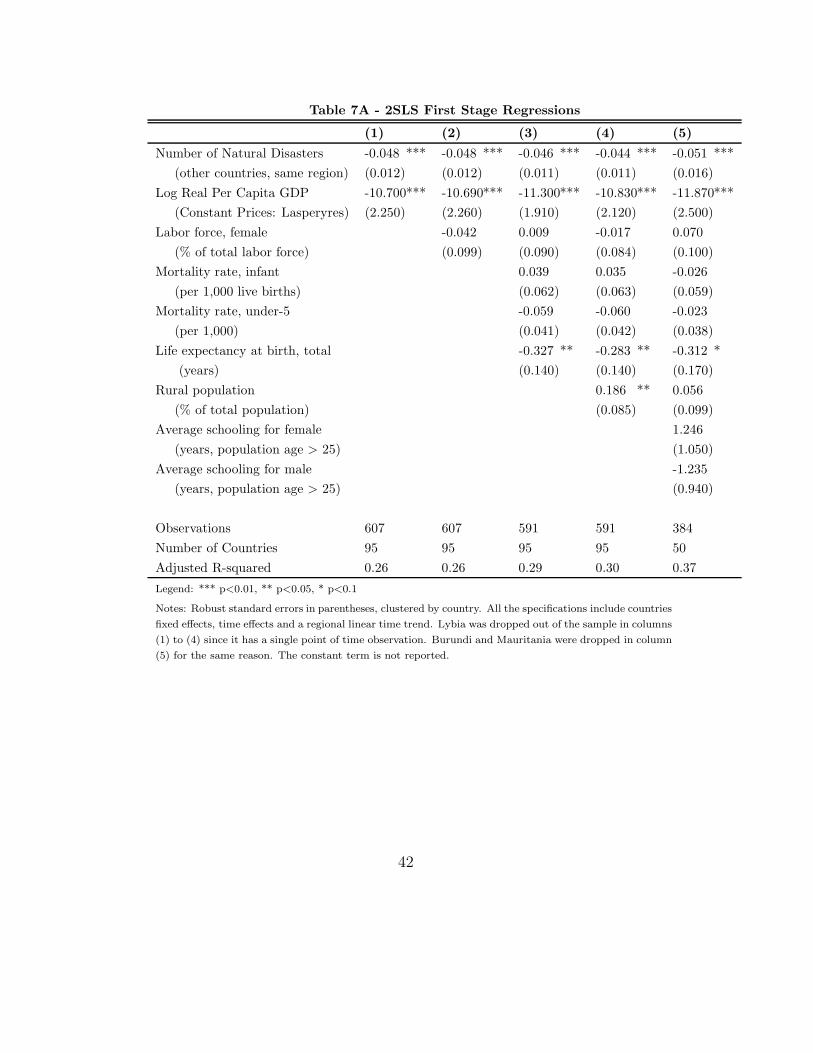
Table 7A - 2SLS First Stage Regressions

(1) (2) (3) (4) (5)

Number of Natural Disasters -0.048 *** -0.048 *** -0.046 *** -0.044 *** -0.051 ***(other countries, same region) (0.012) (0.012) (0.011) (0.011) (0.016)

Log Real Per Capita GDP -10.700*** -10.690*** -11.300*** -10.830*** -11.870***(Constant Prices: Lasperyres) (2.250) (2.260) (1.910) (2.120) (2.500)

Labor force, female -0.042 0.009 -0.017 0.070(% of total labor force) (0.099) (0.090) (0.084) (0.100)

Mortality rate, infant 0.039 0.035 -0.026(per 1,000 live births) (0.062) (0.063) (0.059)

Mortality rate, under-5 -0.059 -0.060 -0.023(per 1,000) (0.041) (0.042) (0.038)

Life expectancy at birth, total -0.327 ** -0.283 ** -0.312 *(years) (0.140) (0.140) (0.170)

Rural population 0.186 ** 0.056(% of total population) (0.085) (0.099)

Average schooling for female 1.246(years, population age > 25) (1.050)

Average schooling for male -1.235(years, population age > 25) (0.940)

Observations 607 607 591 591 384Number of Countries 95 95 95 95 50Adjusted R-squared 0.26 0.26 0.29 0.30 0.37

Legend: *** p<0.01, ** p<0.05, * p<0.1

Notes: Robust standard errors in parentheses, clustered by country. All the specifications include countries

fixed effects, time effects and a regional linear time trend. Lybia was dropped out of the sample in columns

(1) to (4) since it has a single point of time observation. Burundi and Mauritania were dropped in column

(5) for the same reason. The constant term is not reported.

42

Table 7B - 2SLS Results

(1) (2) (3) (4) (5)

ODA and Official Aid 0.045 * 0.044 * 0.045 * 0.040 0.054 **(% GDP) (0.024) (0.024) (0.024) (0.025) (0.025)

Log Real Per Capita GDP 0.208 0.194 0.331 0.329 0.533 *(Constant Prices: Lasperyres) (0.310) (0.310) (0.310) (0.310) (0.310)

Labor force, female 0.022 0.012 0.010 -0.005(% of total labor force) (0.021) (0.017) (0.017) (0.016)

Mortality rate, infant -0.000 -0.001 -0.003(per 1,000 live births) (0.006) (0.006) (0.006)

Mortality rate, under-5 0.004 0.004 0.008 ***(per 1,000) (0.004) (0.004) (0.003)

Life expectancy at birth, total 0.027 * 0.030 ** 0.021(years) (0.015) (0.014) (0.015)

Rural population 0.018 * 0.013(% of total population) (0.010) (0.011)

Average schooling for female -0.344 ***(years, population age > 25) (0.120)

Average schooling for male -0.068(years, population age > 25) (0.140)

Observations 607 607 591 591 384Number of Countries 95 95 95 95 50Adjusted R-squared 0.72 0.72 0.75 0.76 0.80First Stage F Test 16.74 16.56 18.38 15.71 10.09

Legend: *** p<0.01, ** p<0.05, * p<0.1

Notes: Robust standard errors in parentheses, clustered by country. All the specifications include countries

fixed effects, time effects and a regional linear time trend. Lybia was dropped out of the sample in columns

(1) to (4) since it has a single point of time observation. Burundi and Mauritania were dropped in column

(5) for the same reason. The constant term is not reported.

43

Table

8-

2SLS

Regressio

ns

on

the

Effect

ofForeig

nA

idon

severaleconom

icoutcom

es

(1)

(2)

(3)

(4)

(5)

(6)

(7)

Labor

Forc

e(%

Tota

lPopula

-ti

on)

Fem

ale

Labor

Forc

e(%

Tota

lLabor

Forc

e)

Infa

nt

Mort

ality

Rate

,In

fant

Life

Expecta

ncy

at

Bir

thA

vera

ge

School-

ing,Years

Share

of

Invest

-m

ent

ofth

eR

eal

GD

P

Real

GD

PG

row

thPer

Capit

aO

DA

and

Offi

cia

lA

id0.0

003

0.0

493

0.2

270

0.4

380**

-0.0

165

-0.0

920

0.0

02

(%G

DP),

Inst

rum

ente

d(0

.001)

(0.1

10)

(0.7

60)

(0.2

20)

(0.0

21)

(0.2

10)

(0.0

09)

Log

RealPer

Capit

aG

DP

0.0

124

0.6

680

-3.8

460

3.8

880

0.1

470

-2.8

620

0.0

95

(Const

ant

Pri

ces:

Lasp

ery

res)

(0.0

12)

(1.2

80)

(8.3

40)

(2.6

20)

(0.2

70)

(2.9

60)

(0.1

00)

Obse

rvati

ons

607

607

591

607

393

608

529

Num

ber

ofC

ountr

ies

95

95

95

95

50

95

93

Fir

stSta

ge

FTest

16.7

416.7

414.1

516.7

49.4

617.8

516.4

6Legend:

***

p<

0.0

1,**

p<

0.0

5,*

p<

0.1

Note

s:R

obust

standard

err

ors

inpare

nth

ese

s,clu

stere

dby

countr

y.

All

the

specifi

cati

ons

inclu

de

countr

ies

fixed

effects

,ti

me

effects

and

are

gio

nallinear

tim

etr

end.

InC

olu

mn

(7),

the

realG

DP

covari

ate

corr

esp

onds

toth

ein

itia

lLog

RealPer

Capit

aG

DP.

44

Appendix

−5051015Residuals

−.50.51Residuals

33.

54

4.5

5pe

riod

AF

G

−30−20−1001020Residuals

−4−202Residuals

77.

58

8.5

9pe

riod

ALB

−30−20−1001020Residuals

−1.00e−14 −5.00e−1505.00e−15 1.00e−14Residuals

88.

28.

48.

68.

89

perio

d

AR

M

−30−20−1001020Residuals

−.20.2.4.6Residuals

77.

58

8.5

9pe

riod

AZ

E

−40−200204060Residuals

−10−505Residuals

02

46

810

perio

d

BD

I

−40−200204060Residuals

−4−2024Residuals

02

46

810

perio

d

BE

N

−40−200204060Residuals

−4−2024Residuals

02

46

810

perio

d

BF

A

−20−15−10−505Residuals

−3−2−1012Residuals

24

68

10pe

riod

BG

D

−20−1001020Residuals

−.1−.050.05Residuals

77.

58

8.5

9pe

riod

BG

R

−20−1001020Residuals

−4−20246Residuals

77.

58

8.5

9pe

riod

BIH

−30−20−1001020Residuals

−11Residuals

88.

28.

48.

68.

89

perio

d

BLR

−40−2002040Residuals

−1012Residuals

02

46

810

perio

d

BO

L

−40−200204060Residuals

−1.5−1−.50.51Residuals

24

68

10pe

riod

BW

A

−40−200204060Residuals

−4−2024Residuals

24

68

10pe

riod

CA

F

−150−100−50050Residuals

−.2−.10.1.2.3Residuals

45

67

89

perio

d

CH

N

−40−200204060Residuals

−2024Residuals

02

46

810

perio

d

CIV

−40−200204060Residuals

−2−101Residuals

02

46

810

perio

d

CM

R

−40−200204060Residuals

−4−2024Residuals

02

46

810

perio

d

CO

G

−30−20−1001020Residuals

−.01−.0050.005Residuals

77.

58

8.5

9pe

riod

CZ

E

−10−50510Residuals

−202468Residuals

02

46

810

perio

d

DZ

A

−40−2002040Residuals

−.50.5Residuals

02

46

810

perio

d

EC

U

−10−5051015Residuals

−50510Residuals

02

46

810

perio

d

EG

Y

−40−200204060Residuals

−6−4−2024Residuals

77.

58

8.5

9pe

riod

ER

I

−20−1001020Residuals

−.10.1.2Residuals

77.

58

8.5

9pe

riod

ES

T

−50050Residuals

−3−2−101Residuals

56

78

9pe

riod

ET

H

−30−20−1001020Residuals

−1012Residuals

77.

58

8.5

9pe

riod

GE

O

−40−200204060Residuals

−2−1012Residuals

02

46

810

perio

d

GH

A

−40−200204060Residuals

−4−2024Residuals

56

78

9pe

riod

GIN

−40−200204060Residuals

−1001020Residuals

24

68

10pe

riod

GM

B

−40−200204060Residuals

−20−1001020Residuals

24

68

10pe

riod

GN

B

−40−2002040Residuals

−.50.51Residuals

02

46

810

perio

d

GT

M

−40−2002040Residuals

−2−10123Residuals

02

46

810

perio

d

HN

D

−20−1001020Residuals

−.06−.04−.020.02.04Residuals

77.

58

8.5

9pe

riod

HR

V

−40−2002040Residuals

−4−2024Residuals

24

68

10pe

riod

HT

I

−80−60−40−20020Residuals

−1−.50.51Residuals

24

68

10pe

riod

IDN

−30−20−100Residuals

−.4−.20.2.4.6Residuals

02

46

810

perio

d

IND

−1001020Residuals

−2−10123Residuals

02

46

810

perio

d

ISR

−1001020Residuals

−10−5051015Residuals

24

68

10pe

riod

JOR

−20−1001020Residuals

−.1−.050.05.1.15Residuals

77.

58

8.5

9pe

riod

KA

Z

−40−200204060Residuals

−4−20246Residuals

02

46

810

perio

d

KE

N

−20−1001020Residuals

−20246Residuals

77.

58

8.5

9pe

riod

KG

Z

−50050100Residuals

−10−505Residuals

24

68

10pe

riod

KH

M

−50050100Residuals

−4−2024Residuals

56

78

9pe

riod

LAO

−40−200204060Residuals

−20−1001020Residuals

24

68

10pe

riod

LBR

05101520Residuals

−4−2024Residuals

02

46

810

perio

d

LKA

−40−200204060Residuals

−10−50510Residuals

02

46

810

perio

d

LSO

−20−1001020Residuals

−.10.1.2.3Residuals

77.

58

8.5

9pe

riod

LTU

−20−1001020Residuals

−.10.1.2.3Residuals

77.

58

8.5

9pe

riod

LVA

Figure A1: Detrended changes in Foreign Aid and Natural Disasters in neigh-bor countries, Panel I

45

−10−5051015Residuals

−1−.50.511.5Residuals

02

46

810

perio

d

MA

R

−20−1001020Residuals

−.2−.10.1Residuals

77.

58

8.5

9pe

riod

MD

A

−50050Residuals

−3−2−1012Residuals

02

46

810

perio

d

MD

G

−20−1001020Residuals

−.4−.20.2Residuals

77.

58

8.5

9pe

riod

MK

D

−40−200204060Residuals

−50510Residuals

24

68

10pe

riod

MLI

−50050100Residuals

−4−2024Residuals

56

78

9pe

riod

MN

G

−40−200204060Residuals

−10−50510Residuals

24

68

10pe

riod

MR

T

−40−200204060Residuals

−50510Residuals

02

46

810

perio

d

MW

I

−40−200204060Residuals

−2−1012Residuals

56

78

9pe

riod

NA

M

−40−200204060Residuals

−4−2024Residuals

02

46

810

perio

d

NE

R

−40−2002040Residuals

−.50.5Residuals

02

46

810

perio

d

NG

A

−40−2002040Residuals

−5051015Residuals

02

46

810

perio

d

NIC

−100102030Residuals

−4−2024Residuals

02

46

810

perio

d

NP

L

−1001020Residuals

−1−.50.511.5Residuals

24

68

10pe

riod

OM

N

−505101520Residuals

−1012Residuals

02

46

810

perio

d

PA

K

−40−2002040Residuals

−.4−.20.2.4.6Residuals

02

46

810

perio

d

PA

N

−100−50050Residuals

−1−.50.51Residuals

02

46

810

perio

d

PH

L

−50050100Residuals

−2−1012Residuals

24

68

10pe

riod

PN

G

−30−20−1001020Residuals

−.2−.10.1Residuals

77.

58

8.5

9pe

riod

PO

L

−40−2002040Residuals

−1−.50.51Residuals

02

46

810

perio

d

PR

Y

−30−20−10010Residuals

−.1−.050.05Residuals

77.

58

8.5

9pe

riod

RO

M

−40−30−20−100Residuals

−.050.05.1Residuals

77.

58

8.5

9pe

riod

RU

S

−40−200204060Residuals

−10−50510Residuals

02

46

810

perio

d

RW

A

−40−200204060Residuals

−4−2024Residuals

24

68

10pe

riod

SD

N

−40−200204060Residuals

−4−2024Residuals

02

46

810

perio

d

SE

N

−40−200204060Residuals

−10−50510Residuals

24

68

10pe

riod

SLE

−40−2002040Residuals

−4−20246Residuals

02

46

810

perio

d

SLV

−50−40−30−20−100Residuals

−10−5051015Residuals

34

56

7pe

riod

SO

M

−30−20−1001020Residuals

−.050.05.1Residuals

77.

58

8.5

9pe

riod

SV

K

−20−1001020Residuals

−.020.02.04.06Residuals

77.

58

8.5

9pe

riod

SV

N

−40−200204060Residuals

−3−2−1012Residuals

24

68

10pe

riod

SW

Z

−40−200204060Residuals

−505Residuals

02

46

810

perio

d

TC

D

−40−200204060Residuals

−10−505Residuals

02

46

810

perio

d

TG

O

−30−20−10010Residuals

−.50.511.5Residuals

77.

58

8.5

9pe

riod

TJK

−20−1001020Residuals

−.010.01.02Residuals

77.

58

8.5

9pe

riod

TK

M

−1001020Residuals

−1.5−1−.50.51Residuals

02

46

810

perio

d

TU

N−100−50050

Residuals

−.4−.20.2.4Residuals

24

68

10pe

riod

TU

R

−50050Residuals

−4−20246Residuals

67

89

perio

d

TZ

A

−50050Residuals

−50510Residuals

02

46

810

perio

d

UG

A

−30−20−1001020Residuals

−.050.05.1.15Residuals

77.

58

8.5

9pe

riod

UK

R

−20−1001020Residuals

−.15−.1−.050.05.1Residuals

77.

58

8.5

9pe

riod

UZ

B

−100−50050Residuals

−1−.50.51Residuals

67

89

perio

d

VN

M

−10−5051015Residuals

−.10.1.2.3Residuals

77.

58

8.5

9pe

riod

YE

M

−50050Residuals

−.010.01.02.03Residuals

77.

58

8.5

9pe

riod

ZA

F

−50050Residuals

−10−5051015Residuals

24

68

10pe

riod

ZA

R

−40−200204060Residuals

−10−50510Residuals

02

46

810

perio

d

ZM

B

−40−200204060Residuals

−4−2024Residuals

02

46

810

perio

d

ZW

E

Figure A2: Detrended changes in Foreign Aid and Natural Disasters in neigh-bor countries, Panel II

46

Table

A1

-Lis

tofC

ountr

ies

inth

eB

ase

Sam

ple

Europe

Sub-S

aharan

Afr

ica

Alb

ania

Lit

huania

Ben

inM

adagasc

ar

Arm

enia

Mold

ova

Bots

wana

Mala

wi

Aze

rbaijan

Pola

nd

Burk

ina

Faso

Mali

Bel

aru

sR

om

ania

Buru

ndi**

Mauri

tania

**

Bosn

iaand

Her

zegov

ina

Russ

ian

Fed

erati

on

Cam

eroon

Nam

ibia

Bulg

ari

aSlo

vakia

Cen

tralA

fric

an

Rep

ublic

Nig

erC

roati

aSlo

ven

iaC

had

Nig

eria

Cze

chR

epublic

Tajikis

tan

Congo

Rw

anda

Est

onia

Mace

donia

(FY

R)

Cte

d’Ivoir

eSen

egal

Geo

rgia

Turk

eyD

em.

Rep

.ofth

eC

ongo

Sie

rra

Leo

ne

Kaza

khst

an

Turk

men

ista

nE

ritr

eaSom

alia

Kyrg

yzs

tan

Ukra

ine

Eth

iopia

South

Afr

ica

Latv

iaU

zbek

ista

nG

am

bia

Sudan

Ghana

Sw

azi

land

Guin

eaTogo

Guin

ea-B

issa

uU

ganda

Ken

ya

Unit

edR

ep.

ofTanza

nia

Les

oth

oZam

bia

Lib

eria

Zim

babw

e

Lati

nA

meric

a&

Carib

bean

East

Asi

aand

the

Pacifi

cM

iddle

East

and

North

Afr

ica

South

Asi

a

Bolivia

Cam

bodia

Alg

eria

Afg

hanis

tan

Ecu

ador

Chin

aE

gypt

Sri

Lanka

ElSalv

ador

Indones

iaIs

rael

Nep

al

Guate

mala

Lao

PD

RJord

an

Bangla

des

hH

ait

iM

ongolia

Lib

yan

Ara

bJam

ahir

iya*

Pakis

tan

Hondura

sPapua

New

Guin

eaM

oro

cco

India

Nic

ara

gua

Philip

pin

esO

man

Panam

aV

iet

Nam

Tunis

iaPara

guay

Yem

enN

ote

s:C

ountr

ies’

regio

ns

are

defi

ned

by

the

Worl

dB

ank.

All

countr

ies

wer

enev

ernet

donors

bet

wee

n1960-2

004.

All

countr

ies

hav

ea

popula

tion

of

at

least

am

illion

peo

ple

,bet

wee

n1960

and

2004.

*In

dic

ate

sa

countr

yw

ith

only

one

obse

rvati

on

inth

ebase

data

set.

**

Indic

ate

sa

countr

yw

ith

only

one

obse

rvati

on

inth

ere

duce

ddata

set

47

Table A2 - Summary Statistics, per Country

Country Name Periods Aid

(%GDP)

Real GDP Per

Capita (2000 USD)

Fertility

Rate per

Woman

Albania 3 13.18 3069.88 2.47

Algeria 9 2.44 4851.47 5.76

Armenia 2 11.38 3511.92 1.39

Azerbaijan 3 3.04 3173.67 2.29

Bangladesh 7 4.80 1544.91 4.83

Belarus 2 0.44 9672.00 1.28

Benin 9 8.13 1123.56 6.64

Bolivia 9 6.30 2764.76 5.44

Bosnia and Herzegovina 3 23.61 2361.50 1.50

Botswana 7 6.92 4483.15 5.31

Bulgaria 3 1.84 7492.41 1.33

Burkina Faso 9 10.18 785.91 7.03

Burundi 9 14.22 816.74 6.69

Cambodia 5 10.24 541.03 5.14

Cameroon 9 3.89 2357.19 5.91

Central African Republic 7 11.88 965.56 5.48

Chad 9 9.59 892.12 6.51

China 6 0.29 2124.82 2.26

Congo 9 5.86 1791.45 6.24

Croatia 3 0.38 8550.44 1.49

Czech Republic 3 0.40 13157.28 1.36

Cte d’Ivoire 9 3.75 2014.85 6.68

Democratic Republic of the Congo 7 7.41 891.16 6.62

Ecuador 9 1.19 3913.78 4.81

Egypt 9 5.38 2814.36 5.00

El Salvador 9 3.43 3962.55 4.92

Eritrea 3 28.00 601.67 5.73

Estonia 3 1.25 10312.29 1.44

Ethiopia 5 9.20 569.60 6.47

Gambia 8 17.90 908.53 6.04

Georgia 3 6.00 3710.00 1.46

Ghana 9 5.92 1058.52 5.99

Guatemala 9 1.32 3425.11 5.83

Guinea 5 7.75 2388.92 5.96

Guinea-Bissau 7 37.56 627.59 7.03

Haiti 7 7.73 2045.66 5.41

Honduras 9 5.70 2138.14 5.97

India 9 1.05 1614.61 4.73

Indonesia 8 1.85 2509.89 3.94

Israel 9 2.82 14829.25 3.30

Jordan 8 12.98 4189.36 6.06

Kazakhstan 3 0.57 7394.51 2.15

Kenya 9 5.93 1237.94 6.84

Kyrgyzstan 3 11.37 3189.12 2.92

Lao People’s Democratic Republic 5 11.71 1228.14 5.80

Notes: Period is the number of five-years periods for which the data of the is available.

48

Table A2 - Summary Statistics, per Country (Cont.)

Country Name Periods Aid

(%GDP)

Real GDP Per

Capita (2000 USD)

Fertility

Rate per

Woman

Latvia 3 1.10 8197.89 1.37

Lesotho 9 16.68 1166.84 5.29

Liberia 7 21.67 1131.51 6.69

Libyan Arab Jamahiriya 1 0.03 10334.85 3.27

Lithuania 3 1.12 8710.31 1.50

Madagascar 9 7.58 1069.44 6.30

Malawi 9 16.68 655.73 7.05

Mali 8 14.83 835.86 7.09

Mauritania 7 21.05 1328.56 6.00

Moldova 3 4.38 2586.60 1.71

Mongolia 5 10.41 1562.89 3.90

Morocco 9 2.80 2998.04 5.19

Namibia 5 3.09 5072.57 5.44

Nepal 9 6.39 1042.35 5.44

Nicaragua 9 10.76 4873.86 5.68

Niger 9 10.51 1036.58 7.83

Nigeria 9 0.60 1051.48 6.58

Oman 7 1.30 12933.36 7.27

Pakistan 9 3.91 1732.15 6.27

Panama 9 1.39 5484.65 3.97

Papua New Guinea 7 11.82 3676.63 5.36

Paraguay 9 1.89 4175.97 5.18

Philippines 9 1.29 2975.79 4.90

Poland 3 1.23 7541.47 1.57

Romania 3 0.92 5326.03 1.38

Russian Federation 3 0.39 9675.42 1.37

Rwanda 9 15.72 1048.66 7.54

Senegal 9 9.16 1480.80 6.46

Sierra Leone 7 13.44 1117.87 6.38

Slovakia 3 0.61 9213.72 1.53

Slovenia 3 0.25 16493.44 1.29

Somalia 5 38.79 1155.72 7.23

South Africa 3 0.30 7908.79 3.04

Sri Lanka 9 4.58 2242.28 3.38

Sudan 7 4.61 1074.06 5.69

Swaziland 7 5.07 6268.80 5.57

Tajikistan 3 8.17 1832.85 3.75

Macedonia (FRY) 3 3.81 5051.28 1.92

Togo 9 8.39 1033.27 6.39

Tunisia 9 3.93 4399.47 4.74

Turkey 8 0.48 4232.69 3.88

Turkmenistan 3 0.89 6989.42 3.23

Uganda 9 7.67 899.04 6.98

Ukraine 3 0.87 5687.46 1.38

United Republic of Tanzania 4 17.85 633.80 5.78

Uzbekistan 3 0.98 3575.10 3.14

Viet Nam 4 3.30 1825.19 2.96

Yemen 3 4.80 1007.28 6.65

Zambia 9 11.02 1082.16 6.53

Zimbabwe 9 2.38 2962.93 5.96

Notes: Period is the number of five-years periods for which the data of the is available.

49

Table A3 - Number of Natural Disasters per Country

Country Name Total Disasters (1960-2004)

Afghanistan 9

Albania 8

Algeria 50

Armenia 4

Azerbaijan 9

Bangladesh 173

Belarus 3

Benin 12

Bolivia 36

Bosnia and Herzegovina 5

Botswana 5

Bulgaria 6

Burkina Faso 7

Burundi 9

Cambodia 10

Cameroon 10

Central African Republic 10

Chad 9

China 392

Congo 5

Croatia 3

Czech Republic 6

Cte d’Ivoire 2

Democratic Republic of the Congo 17

Ecuador 49

Egypt 18

El Salvador 22

Eritrea 3

Estonia 0

Ethiopia 30

Gambia 5

Georgia 10

Ghana 8

Guatemala 38

Guinea 5

Guinea-Bissau 4

Haiti 40

Honduras 36

India 314

Indonesia 237

Israel 5

Jordan 8

Kazakhstan 6

Kenya 21

Kyrgyzstan 11

Lao People’s Democratic Republic 15

Latvia 1

50

Table A3 - Number of Natural Disasters per Country (Cont.)

Country Name Total Disasters (1960-2004)

Lesotho 8

Liberia 3

Libyan Arab Jamahiriya 0

Lithuania 2

Madagascar 34

Malawi 19

Mali 9

Mauritania 10

Moldova 6

Mongolia 13

Morocco 24

Namibia 4

Nepal 49

Nicaragua 34

Niger 10

Nigeria 29

Oman 5

Pakistan 85

Panama 28

Papua New Guinea 35

Paraguay 16

Philippines 329

Poland 8

Romania 29

Russian Federation 66

Rwanda 7

Senegal 13

Sierra Leone 5

Slovakia 7

Slovenia 2

Somalia 7

South Africa 33

Sri Lanka 44

Sudan 22

Swaziland 2

Tajikistan 28

Macedonia (FRY) 5

Togo 6

Tunisia 12

Turkey 83

Turkmenistan 2

Uganda 21

Ukraine 13

United Republic of Tanzania 23

Uzbekistan 2

Viet Nam 85

Yemen 16

Zambia 8

Zimbabwe 6

51

Table A5 - 2SLS Results Including Net Donors and Large Countries

(1) (2) (3) (4) (5)

ODA and Official Aid 0.059 * 0.058 * 0.049 * 0.046 0.054(% GDP) (0.033) (0.031) (0.028) (0.028) (0.034)Log Real Per Capita GDP 0.365 0.331 0.367 0.380 0.476(Constant Prices: Lasperyres) (0.290) (0.270) (0.240) (0.240) (0.300)Labor force, female 0.005 -0.003 -0.003 0.001(% of total labor force) (0.014) (0.013) (0.013) (0.016)Mortality rate, infant 0.001 0.002 -0.003(per 1,000 live births) (0.007) (0.007) (0.006)Mortality rate, under-5 0.006 0.005 0.010 ***(per 1,000) (0.004) (0.004) (0.004)Life expectancy at birth, total 0.027 * 0.030 ** 0.024(years) (0.015) (0.014) (0.016)Rural population 0.020 ** 0.021 **(% of total population) (0.008) (0.009)Average schooling for female -0.312 ***(years, population above age 25) (0.100)Average schooling for male 0.029(years, population above age 25) (0.120)

Observations 1,009 970 908 908 592Number of Countries 154 148 145 145 78Adjusted R-squared 0.63 0.65 0.73 0.74 0.78First Stage F Test 7.018 10.03 10.16 9.907 8.236

Legend: *** p<0.01, ** p<0.05, * p<0.1

Notes: Robust standard errors in parentheses, clustered by country. All the specifications include countries

fixed effects, time effects and a regional linear time trend.

52

Table A5 - 2SLS Results Including Large Countries

(1) (2) (3) (4) (5)

ODA and Official Aid 0.043 0.043 * 0.045 * 0.042 * 0.051 **(% GDP) (0.026) (0.025) (0.024) (0.025) (0.025)Log Real Per Capita GDP 0.352 0.291 0.393 0.400 0.474(Constant Prices: Lasperyres) (0.310) (0.280) (0.280) (0.280) (0.300)Labor force, female 0.020 0.011 0.009 0.007(% of total labor force) (0.015) (0.013) (0.012) (0.013)Mortality rate, infant 0.001 0.001 -0.004(per 1,000 live births) (0.007) (0.007) (0.005)Mortality rate, under-5 0.004 0.004 0.008 ***(per 1,000) (0.004) (0.004) (0.003)Life expectancy at birth, total 0.028 * 0.031 ** 0.020(years) (0.015) (0.014) (0.015)Rural population 0.019 ** 0.015(% of total population) (0.008) (0.011)Average schooling for female -0.328 ***(years, population above age 25) (0.120)Average schooling for male -0.056(years, population above age 25) (0.140)

Observations 727 697 669 669 396Number of Countries 117 112 111 111 52Adjusted R-squared 0.66 0.69 0.73 0.74 0.80First Stage F Test 6.651 10.31 10.27 9.707 9.361

Legend: *** p<0.01, ** p<0.05, * p<0.1

Notes: Robust standard errors in parentheses, clustered by country. All the specifications include countries

fixed effects, time effects and a regional linear time trend.

53

Table A5 - 2SLS Results Excluding Egypt and Israel

(1) (2) (3) (4) (5)

ODA and Official Aid 0.042 * 0.041 * 0.040 * 0.038 0.048 *(% GDP) (0.022) (0.022) (0.023) (0.024) (0.025)Log Real Per Capita GDP 0.123 0.118 0.218 0.227 0.366(Constant Prices: Lasperyres) (0.300) (0.300) (0.320) (0.310) (0.320)Labor force, female 0.006 0.002 -0.000 -0.007(% of total labor force) (0.015) (0.013) (0.014) (0.016)Mortality rate, infant 0.000 -0.000 -0.004(per 1,000 live births) (0.006) (0.006) (0.005)Mortality rate, under-5 0.002 0.002 0.007 **(per 1,000) (0.004) (0.004) (0.003)Life expectancy at birth, total 0.028 * 0.030 ** 0.019(years) (0.014) (0.014) (0.015)Rural population 0.011 0.007(% of total population) (0.011) (0.012)Average schooling for female -0.325 ***(years, population above age 25) (0.120)Average schooling for male -0.008(years, population above age 25) (0.130)

Observations 589 589 575 575 371Number of Countries 93 93 93 93 48Adjusted R-squared 0.75 0.75 0.78 0.78 0.82First Stage F Test 18.54 18.27 19.31 16.94 9.642

Legend: *** p<0.01, ** p<0.05, * p<0.1

Notes: Robust standard errors in parentheses, clustered by country. All the specifications include countries

fixed effects, time effects and a regional linear time trend.

54

References

[1] Alberto Alesina and David Dollar. Who gives foreign aid to whom and

why? Journal of Economic Growth, 5(1):33–63, March 2000.

[2] Leonid V. Azarnert. Foreign aid, fertility and human capital accumula-

tion. Economica, 2008.

[3] Robert J. Barro. Economic growth in a cross section of countries. The

Quarterly Journal of Economics, 106(2):407–443, 1991.

[4] Robert J. Barro and Jong-Wha Lee. International data on educational

attainment updates and implications. NBER Working Papers 7911,

National Bureau of Economic Research, Inc, September 2000.

[5] Gary S. Becker and H. Gregg Lewis. On the interaction between the

quantity and quality of children. The Journal of Political Economy,

81(2):S279–S288, 1973.

[6] Gary S. Becker, Kevin M. Murphy, and Robert Tamura. Human capi-

tal, fertility, and economic growth. The Journal of Political Economy,

98(5):S12–S37, 1990.

[7] J.R. Behrman, S. Duryea, and M. Szekely. Decomposing fertility dif-

ferences across world regions and over time: Is improved health more

important than women’s schooling? (406), 1999.

[8] Nancy Birdsall. Economic approaches to population growth. In Hollis

Chenery and T.N. Srinivasan, editors, Handbook of Development Eco-

nomics.

[9] Peter Boone. Politics and the effectiveness of foreign aid. European

Economic Review, 40(2):289–329, February 1996.

55

[10] James A. Brander and Steve Dowrick. The role of fertility and popula-

tion in economic growth: Empirical resultsfrom aggregate cross-national

data. NBER Working Papers 4270, National Bureau of Economic Re-

search, Inc, February 1993.

[11] Craig Burnside and David Dollar. Aid, policies, and growth. American

Economic Review, 90(4):847–868, September 2000.

[12] Charles Cohen and Eric Werker. The political economy of ”natural”

disasters. HBS Working Paper Series, (08-040), December 2007.

[13] Paul Collier and David Dollar. Aid allocation and poverty reduction.

European Economic Review, 46(8):1475–1500, September 2002.

[14] Paul Collier and David Dollar. Development effectiveness: what have

we learnt? Economic Journal, 114(496):F244–F271, 06 2004.

[15] Paul Collier and Anke Hoeffler. Aid, policy, and growth in post-conflict

societies. Policy Research Working Paper Series 2902, The World Bank,

October 2002.

[16] Carl-Johan Dalgaard, Henrik Hansen, and Finn Tarp. On the empirics

of foreign aid and growth. Economic Journal, 114(496):F191–F216, 06

2004.

[17] William Easterly. The White Man’s Burden: Why the West’s Efforts to

Aid the Rest Have Done So Much Ill and So Little Good. Penguin Press,

2006.

[18] William Easterly, Ross Levine, and David Roodman. Aid, policies, and

growth: Comment. American Economic Review, 94(3):774–780, June

2004.

[19] EM-DAT. Em-dat: The ofda/cred international disaster database -

www.emdat.net, 2008.

56

[20] Milton Friedman. Foreign economic aid: Means and objectives. Yale

Review, 47(4):500, 1958.

[21] Oded Galor and David N. Weil. Population, technology, and growth:

From malthusian stagnation to the demographic transition and beyond.

The American Economic Review, 90(4):806–828, 2000.

[22] P. Guillaumont and L. Chauvet. Aid and performance: A reassessment.

The Journal of Development Studies, 37(6):66–92, August 2001.

[23] Henrik Hansen and Finn Tarp. Aid and growth regressions. Journal of

Development Economics, 64(2):547–570, April 2001.

[24] Garrett Hardin. Lifeboat ethics: the case against helping the poor.

Psychology Today, pages 38–43, September 1974a.

[25] Garrett Hardin. Living on a lifeboat. Bioscience, 24(10):561–568, 1974b.

[26] Alan Heston, Robert Summers, and Bettina Aten. Penn world table

version 6.2, September 2006.

[27] Ilyana Kuziemko and Eric Werker. How much is a seat on the security

council worth? foreign aid and bribery at the united nations. Journal

of Political Economy, 114(5):905–930, October 2006.

[28] Alfred Maizels and Machiko K. Nissanke. Motivations for aid to devel-

oping countries. World Development, 12(9):879–900, September 1984.

[29] Thomas Robert Malthus. An Essay on the Principle of Population.

History of Economic Thought Books. McMaster University Archive for

the History of Economic Thought, 1798.

[30] Omer Moav. Cheap children and the persistence of poverty. Economic

Journal, 115(500):88–110, 01 2005.

57

[31] Paul Mosley, John Hudson, and Sara Horrell. Aid, the public sector and

the market in less developed countries. Economic Journal, 97(387):616–

41, September 1987.

[32] Larry Nowels and Curt Tarnoff. Foreign aid: An introductory overview

of u.s. programs and policy. Crs report for congress, US Congressional

Research Service, April 2004.

[33] Gustav F Papanek. Aid, foreign private investment, savings, and growth

in less developed countries. Journal of Political Economy, 81(1):120–30,

Jan.-Feb. 1973.

[34] David Roodman. The anarchy of numbers: Aid, development, and cross-

country empirics. (0412003), 2007.

[35] Jeffrey D. Sachs. The End of Poverty: Economic Possibilities for Our

Time. Penguin Press, 2005.

[36] Robert M. Solow. A contribution to the theory of economic growth. The

Quarterly Journal of Economics, 70(1):65–94, 1956.

[37] William N. Trumbull and Howard J. Wall. Estimating aid-allocation cri-

teria with panel data. The Economic Journal, 104(425):876–882, 1994.

[38] USAID. Congressional Budget Justification for Foreign Operations, Fis-

cal Year 2009. 2008.

[39] The World Bank. Assessing Aid: What Works, What Doesn’t and Why.

1998.

[40] The World Bank. World Development Indicators 2005. World Bank,

2005.

[41] The World Bank. World Development Indicators 2007. World Bank,

2007.

58