cigre 467 - economic framework for power quality
TRANSCRIPT

8/20/2019 CIGRE 467 - Economic Framework for Power Quality
http://slidepdf.com/reader/full/cigre-467-economic-framework-for-power-quality 1/151
467
Economic Framework For Power Quality
CIGRE/CIRED
Joint Working GroupC4.107
June 2011

8/20/2019 CIGRE 467 - Economic Framework for Power Quality
http://slidepdf.com/reader/full/cigre-467-economic-framework-for-power-quality 2/151
Economic Framework for Power Quality
JWG CIGRE-CIRED C4.107
Members
Jose Gutierrez Iglesias (ES) - (Convener), Detmar Arlt (DE), Gerhard Bartak (AT),Math Bollen (SE),Dave Byrne (EI), David Chapman (UK), Alice Delahunty (UK),
Philippe Eyrolles (FR), Elena Fumagalli (IT), Mats Hager (SE), Zbigniew Hanzelka (PL),Bill Howe (US), Rafaël Jahn (BE), Alex McEachern (US), Ian McMichael (AU),
Jovica V. Milanovic (UK), Patxi Pazos (ES), Roman Targosz (PL), MarioTremblay (CN),Jasper Van Casteren (NL), Mathieu Van Den Bergh (US),
Raghavan Venkatesh (IN), Paola Verde (IT)
Copyright © 2011
“Ownership of a CIGRE publication, whether in paper form or on electronic support only infers right ofuse for personal purposes. Are prohibited, except if explicitly agreed by CIGRE, total or partialreproduction of the publication for use other than personal and transfer to a third party; hencecirculation on any intranet or other company network is forbidden”.
Disclaimer notice“CIGRE gives no warranty or assurance about the contents of this publication, nor does it accept anyresponsibility, as to the accuracy or exhaustiveness of the information. All implied warranties andconditions are excluded to the maximum extent permitted by law”.
ISBN: 978- 2- 85873- 157-2
8/20/2019 CIGRE 467 - Economic Framework for Power Quality
http://slidepdf.com/reader/full/cigre-467-economic-framework-for-power-quality 3/151
2
EXECUTIVE SUMMARY
Electric power quality disturbances can have significant economic consequences for many different types
of facilities. Although power quality is widely recognized as an important issue, there is no consensus onits total economic impact. Indeed, there is not even consensus on how to measure the impact.
A wide range of potential solutions, with varying degrees of cost and effectiveness, are available tomitigate the consequences associated with poor power quality. Power quality solutions can be applied atdifferent levels or locations within the global electrical system.
The evaluation of power quality improvement alternatives is an exercise in economics. Facility managersand utility engineers must evaluate the economic impacts of the power quality variations against the costsof improving performance for the different alternatives. The best choice will depend on the costs of the
problem and the total operating costs of the various solutions.
In general, the costs of these solutions increase as the power level of the load that must be protectedincreases. This means that economies usually can be achieved if sensitive equipment or controls can beisolated and protected individually from equipment that does not need protection.
Each solution technology needs to be characterized in terms of cost and effectiveness. In broad terms, thesolution cost should include initial procurement and installation expenses, operating and maintenanceexpenses, and any disposal and/or compensation value considerations.
Improving facility performance during power quality variations can result in significant savings and can be a competitive advantage. Therefore, it is important for customers and suppliers to work together inidentifying the best alternative for achieving the required level of performance.
A methodology for performing a comparative economic analysis is featured in this report.
A joint working group, JWG C4.107, has been formed between CIGRE (electric power transmissionemphasis) and CIRED (electric power distribution emphasis) to develop a systematic approach to thisissue.
The JWG works to develop a framework for analysis of the economics of power quality, and has created a bibliography of existing references. However, gathering specific values and data to assess the economicsof power quality is beyond the scope of the Group; the work will be limited to developing a framework.
Different technologies are evaluated by estimating the improved performance that can be expected afterthe technology has been applied. The power quality cost savings are calculated for each technology alongwith the costs of applying the technology.
JWG C4.107 aimed to produce this report that summarizes available information about cost-benefitanalysis of power quality, and to propose a framework for how to assess costs, how to assess theeconomic impact of mitigation, and how to assess the economic impact of immunity.

8/20/2019 CIGRE 467 - Economic Framework for Power Quality
http://slidepdf.com/reader/full/cigre-467-economic-framework-for-power-quality 4/151
3
TABLE OF CONTENTS
EXECUTIVE SUMMARY........................................................................................................................2
1. Introduction to the Economics of Power Quality ................................................................. ............5
1.1. SCOPE OF THE REPORT ....................................................... .......................................................... ..5 1.1.1. The Economic Importance of Power Quality............................................................................5 1.2. ECONOMIC CONSEQUENCES OF POOR PQ FOR END USERS .................................................. 6 1.3. ECONOMICS OF POWER QUALITY FOR POWER NETWORKS ................................................. 7 1.4. ECONOMICS OF POWER QUALITY FOR SOCIETY .............................................................. .......8 1.5. ROLE OF REGULATION....................................................................................................................9 1.6. OVERVIEW OF THE DOCUMENT ......................................................... ........................................ 10
2. Overview of Methodologies for Assessment of Economic Impact – End User Perspective.........12 2.1. METHODOLOGY FOR QUANTIFYING THE ECONOMIC IMPACT OF VOLTAGE SAGS ANDSHORT INTERRUPTIONS.......................................................................................................................12
2.1.1. Introduction.............................................................................................................................12 2.1.2. Overview of Existing Methodologies ..................................................................... ................12 2.1.3. IEEE Guidelines......................................................................................................................14 2.1.4. Analytical Economic Analysis................................................................................................14 2.1.5. Indirect Economic Analysis....................................................................................................17 2.1.6. Reported PQ-Related Losses from Around the World............................................................19
2.2. METHODOLOGY FOR QUANTIFYING THE ECONOMIC IMPACT OF HARMONICS ...........23 2.2.1. Introduction.............................................................................................................................23 2.2.2. Overview of Existing Methodologies ..................................................................... ................24
2.3. METHODOLOGY FOR QUANTIFYING THE ECONOMIC IMPACT OF OTHER PQPHENOMENA...........................................................................................................................................29
2.3.1. Voltage and Current Unbalance..............................................................................................29 2.3.2. Surges and Transients ................................................................... .......................................... 34 2.3.3. Flicker .......................................................... ................................................................. ..........35
2.4. CONCLUSIONS.................................................................................................................................36
3. Overview of Existing Methodologies for Assessment of Economic Impact – Public Distribution
Network Perspective.................................................................................................................................37 3.1. INTRODUCTION...............................................................................................................................37 3.2. REVIEW OF LITERATURE AND DOCUMENTED METHODOLOGIES.....................................38 3.3. COSTS ASSOCIATED WITH PQ ....................................................... .............................................. 38
3.3.1. Costs Incurred by the Utility to Mitigate PQ Issues................................................................39 3.3.2. Costs Associated with Improving Reliability but not PQ ....................................................... 45 3.3.3. Costs for Responding to PQ Issues .......................................................... ............................... 46
3.4. SUMMARY ......................................................... ........................................................... ....................47 3.5. CONCLUSIONS.................................................................................................................................47
4. Methodology for Collecting Power Quality Economic Data.......................................................... 49 4.1. INTRODUCTION...............................................................................................................................49 4.2. IMPORTANCE AND MOTIVATION .............................................................. ................................. 49 4.3. END-USER PERSPECTIVE ........................................................... ................................................... 50
4.3.1. Technical Data .............................................................. ........................................................ ..50 4.3.2. Economic Data........................................................................................................................52
4.4. DNO PERSPECTIVE: DATA COLLECTION ............................................................. .....................60 4.5. CONCLUSIONS.................................................................................................................................62
5. Methodology for the Economic Assessment of Power Quality Solutions......................................63 5.1. INTRODUCTION...............................................................................................................................63 5.2. ECONOMIC ANALYSIS OF THE COSTS OF PQ...........................................................................63
5.2.1. Economic Impact of Power Quality Variations ..................................................................... .63 5.3. END-USE PQ SOLUTIONS...............................................................................................................71 5.4. CHOOSING THE OPTIMAL PQ SOLUTION..................................................................................79
5.5. CONCLUSION ........................................................ ........................................................ ...................80 APPENDIX 1 ................................................... ........................................................... .............................. 81

8/20/2019 CIGRE 467 - Economic Framework for Power Quality
http://slidepdf.com/reader/full/cigre-467-economic-framework-for-power-quality 5/151
4
A COMMON PQ PHENOMENA.......................................................................................................81 A.1 Categories of Power Quality Variations ............................................................... ..............81
B RESPONSE OF SENSITIVE EQUIPMENT TO PQ EVENTS......................................................87 B.1 Data Processing and Communications Equipment.............................................................87 B.2 Variable-Speed Drives........................................................................................................88 B.3 Lighting ............................................................ ................................................................. .88
B.4 Solenoid-Operated Contactors............................................................................................89 C ADDITIONAL LOSSES CAUSED BY POOR PQ........................................................................89 C.1 Cables ........................................................ ................................................................ .........89 C.2 Transformers.......................................................................................................................90 C.3 Motors ........................................................ ........................................................... .............90
APPENDIX 2 ................................................... ........................................................... .............................. 91 A OVERVIEW OF INTERRUPTION COST CALCULATION........................................................91 B PROBABILISTIC VOLTAGE DIP COSTS CALCULATION......................................................92 C OVERVIEW OF EQUIPMENT SENSITIVITY.............................................................................92 D UNCERTAINTY INVOLVED WITH EQUIPMENT SENSITIVITY..........................................93 E COUNTING OF PROCESS TRIPS .................................................................. .............................. 94 F COST ASSESSMENT.....................................................................................................................96 G NUMERICAL EXAMPLE............................ ................................................................ .................96
I TYPICAL LOSS VALUES...........................................................................................................102 J TYPICAL FINANCIAL LOSS VALUES - SUMMARY.............................................................108 K FORMULAE FOR COMPUTING HARMONIC LOSSES FOR THE MAIN ELECTRICALCOMPONENTS.......................................................................................................................................113 L METHODS FOR PROBABILISTIC EVALUATIONS................................................................116 APPENDIX 3 ................................................... ........................................................... ............................ 123 A COST ASPECTS...........................................................................................................................123 B HYDRO-QUEBEC-IREQ REPORT FOR ECONOMICAL ASPECT OF HARMONICS ONDISTRIBUTION AND TRANSMISSION SYSTEM ................................................................. ............128
B.1 Harmonics Power Losses Evaluation.......................................................................................128 B.2 Harmonics Losses Evaluation .................................................................. ................................ 128 B.3 Harmonic Losses Cost Evaluation............................................................................................129 B.4 Conclusion................................................................................................................................129
APPENDIX 4 ................................................... ........................................................... ............................ 131 A STRUCTURING THE DATA COLLECTION PROCESS .......................................................... 131 B EXECUTING DATA COLLECTION PROCESS – END USER PERSPECTIVE ...................... 133 C CONCLUSIONS .................................................... ........................................................... ............134 APPENDIX 5 ................................................... ........................................................... ............................ 136 A ILLUSTRATIVE CASE STUDY .............................................................. ................................... 136
A.1 Base Case: Facility Data and Base Case Calculations......................................................136 A.2 Case 1: Redundancy in the Utility Supply........................................................................137 A.3 Case 2: Applying a Battery UPS ........................................................... ........................... 138 A.4 Case 4: Using Distributed Energy Resources (DER) ....................................................... 140
B CASE COMPARISON AND SENSITIVITY...............................................................................141 REFERENCES........................................................ .............................................................. .................143 ACKNOWLEDGMENTS......................................................................................................................150

8/20/2019 CIGRE 467 - Economic Framework for Power Quality
http://slidepdf.com/reader/full/cigre-467-economic-framework-for-power-quality 6/151
5
1. Introduction to the Economics of Power Quality
1.1. Scope of the Report
Various independent studies have been undertaken by power companies, consultants, regulators, andresearch organizations to estimate the cost of power quality problems to the power companies and theircustomers. A good understanding of the basis for determining these costs is important in assessingappropriate interventions (either by the distribution network operator or by the customers themselves).
A joint working group has been launched with CIRED, where the question has been a subject of a 2001round-table discussion. This is supported by the convener of CIRED S2 (EMC & Power Quality).
The scope of the proposed JWG was to:
• Review and document the economic implications of the power quality parameters: voltage dips, short
interruptions, and voltage waveform quality. Long interruptions were not considered.
• Review and document methods of assessing these costs that have been used to date, including aspectssuch as:
I. Direct and indirect costs to customers (e.g. production losses and plant damage).II. Energy losses associated with poor power quality.
III. Cost of energy not supplied.IV. Methods of collecting customer costs.V. Actual customer costs collected to date for various industry sectors.
• Propose a standardized method of collecting the above information, based on the experience ofvarious international studies.
• Recommend a methodology of using this data to cost and motivate power quality interventions on the power system or within the customer plant.
• Provide indicative costs for specific industry sectors, where possible.
Many professionals, including industry regulators, consultants, system and installation designers,maintenance managers, production managers, and financial mangers, are concerned about the impact ofthe costs of poor power quality on businesses and how these costs can be managed. Techniques foravoiding or reducing the impact of power quality issues are well known and the cost of their deploymentrelatively easily determined. However, assessing the potential cost impact of power quality (PQ) issues isdifficult because, for example, the incidence of problems, the response of equipment, and the effect on
process continuity are statistical in nature and are difficult to quantify. Although there have beennumerous case studies, there has been, so far, no consensus on how the calculation or assessment of these
costs should be approached.
This report provides a methodology for examining the economic framework for PQ. It will enable allinterested parties to establish costs and benefits of PQ improvement and mitigation measures in aconsistent and open manner.
1.1.1. The Economic Importance of Power Quality
“Power quality” is the term generically used to describe the extent to which the electrical power availableat the point of use is compatible with the needs of the load equipment connected at that point. The effectsof a lack of compatibility are termed PQ problems or PQ issues. Compatibility is a two-sided equation
because both the characteristics of the electrical power supply AND the sensitivity of the load equipmentare important variables.
8/20/2019 CIGRE 467 - Economic Framework for Power Quality
http://slidepdf.com/reader/full/cigre-467-economic-framework-for-power-quality 7/151
6
There are many parameters for which compatibility is necessary, including supply voltage level, voltagestability, waveform distortion due to harmonics and interharmonics, voltage unbalance between the
phases, and long- and short-term availability of the supply.
When there is a lack of compatibility, end-user equipment may cease to function, may operate erraticallyor incorrectly, or may operate outside its normal envelope at reduced efficiency or in such a way that its
operating life is reduced. The situation is further complicated by the fact that many PQ issues are caused by the operation (or mis-operation) of end-use equipment that is connected to the network.
Electrical and electronic equipment rarely operate in isolation. Even the simplest of commercialoperations requires the interoperation of several items of equipment—the use of a personal computerusually requires the aid of some communications equipment, a network, and a printer, for example. Inother words, the failure of one piece of equipment usually results in the failure of a process that may ormay not affect other processes. Regardless, however, when process equipment ceases operation, the resultis a financial loss. Depending on factors such as the nature of the business, the organization of the workflow (whether continuous processing or batch production) and the value of the product, this loss mayrange from the trivially small to the extremely large.
There are two obvious approaches to ensuring 100% compatibility between electric power supply and
end-use loads: Either design and construct a perfect electric power delivery grid, or make all end-usedevices perfectly tolerant of common PQ issues. Unfortunately, for a number of reasons, neither of theseapproaches represents the economic optimum. Firstly, some loads are relatively insensitive to many PQ
phenomena while being rather sensitive to others. Incandescent lighting is insensitive to harmonicdistortion but overly sensitive—in combination with the human response—to flicker. On the other hand,electronic equipment is not disturbed by the scale of voltage instability that causes flicker; however, it isvery sensitive to voltage dips and to higher levels of harmonic voltage distortion. Making every supplysuitable for every load would be expensive and is unnecessary. Secondly, although the cost of designingand manufacturing any individual piece of equipment to be “immune” is not large, that cost is multiplied
by the total number of pieces of equipment in use and represents a very large economic burden onconsumers. Thirdly, the option of building a very robust, very clean power system would be extremely highand it would be very difficult, if not impossible, to guarantee a minimum performance level at all points ofcommon coupling. Increased penetration of distributed generation will make this even more difficult as
generation is added at medium and low voltage levels. Lastly, many PQ issues arise within theconsumer’s premises, due to the characteristics of the installed equipment, sub-optimal installation ofequipment and cabling, poor electromagnetic compatibility (EMC) performance of earthing systems, etc.,so perfection at the point of common coupling is no guarantee of adequacy at the point of use.
1.2. Economic Consequences of Poor PQ for End Users
From the descriptions of equipment responses, it is apparent that the economic consequences of poor PQfall into three broad categories:
• Complete or partial loss of one or more processes (e.g.
loss of control following a dip)• Poor long-term productivity or product quality (e.g. as aresult of operator fatigue due to flicker)
• Increased costs due to reduction of equipment lifetimeresulting in premature failure (e.g. overheating oftransformers due to harmonics)
These consequences take effect over very different timescales.
A process failure, triggered by a PQ event such as a dip, hasimmediate consequences followed by a period of recovery,during which further costs may be incurred. It is relatively
easy to identify the costs that result from a single event or to predict what the costs might be.

8/20/2019 CIGRE 467 - Economic Framework for Power Quality
http://slidepdf.com/reader/full/cigre-467-economic-framework-for-power-quality 8/151
7
Continuous or prolonged conditions, such as flicker, can reduce long-term productivity. If the problem is prolonged and widespread, the business may become uncompetitive and may require additional borrowing to sustain it.
Premature failure of equipment will usually result in process failure with similar consequences to thosecaused by single PQ events. The difference is that the causes are in the past and were unrecognized,
suggesting that predicting these costs is difficult unless a survey procedure is put in place.
Depending on the type of operation in question, the economic consequences may range from trivial tocatastrophic. The user can take several approaches:
• Do nothing, and suffer the consequences.• Take responsibility by adding mitigation equipment or hardening measures within the installation.• Work with a supplier to improve the level of PQ by local measures specifically for, but external to,
the installation.• Negotiate with a supplier for a guarantee of a defined level of PQ, along the lines of an insurance
policy.
“Doing nothing”—business as usual—is viable only for those enterprises that use batch processing for
manufacturing and data handling. Process interruptions are limited in their impact and are relatively easilymitigated by, for example, reorganizing work schedules. The economic consequences are not zero but areacceptable to the business.
In every other case, the first steps in analysis of the economic impact of PQ on a particular organizationor part of an organization include:
• Obtaining a thorough and continuing measurements of relevant PQ parameters• Logging of process failures and their costs and relating their occurrence to PQ events• Assessing the likely failure modes and failure rates of processes and items of equipment, bearing in
mind the different time scales involved• Considering options for redesigning processes to reduce interdependence and reduce the risk of
cascading failures• Investigate options for hardening process equipment against PQ events and conditions
1.3. Economics of Power Quality for Power Networks
Network operators are usually required to maintain a certain quality of service to end-users by locallegislation or regulation. Quality of service may be defined by a number of parameters, such asavailability and voltage stability. Achieving the required level requires that the operator invest in, forexample:
a. A monitoring program to identify potential failures (e.g. in transformers) so that repair ormaintenance work can be planned, and unplanned downtime can be avoided
b. Careful planning of maintenance to avoid excess unavailabilityc. Maintenance work to avoid damage to lines, such as tree cutting programs
Network operators need to ensure that consumers are connected appropriately (e.g. at a suitable voltagelevel) to avoid negative impacts on other local consumers from excessive harmonic currents or voltagedisturbances. This usually involves offering consumers pre-connection support so that such issues can beavoided.
Some of the measures taken by utilities and consumers to reduce the impact of power quality issuesrequire the installation of additional equipment. Apart from the obvious cost issue, this equipment hasenvironmental consequences; electrical energy efficiency is reduced. and the additional equipmentconsumes materials and energy for its manufacture. The so-called externalities need to be taken intoaccount.

8/20/2019 CIGRE 467 - Economic Framework for Power Quality
http://slidepdf.com/reader/full/cigre-467-economic-framework-for-power-quality 9/151
8
1.4. Economics of Power Quality for Society
While the economic impact of power quality for users and for utilities is readily identifiable, the impacton society in general is less tangible.
In the recent years, the thrust on sustainable development, clean development mechanisms, and variousother global (green) initiatives have necessitated extrapolating the local and short-term aspects to theglobe and long-term impacts to identify the true holistic impact of industrial activities.
Specific to energy, the focus is shifting from local short-term to global long-term and while computingthe impact of energy conservation it makes sense to consider the energy leverage.
Electrical energy is only an intermediate form of energy used only for bulk power transmission. Due tothis, the role of electrical energy is very critical, and due to the various transformations taking place rightfrom environment to end use, the impact of energy conservation at end use assumes a very highsignificance.
Considering a simple case of power quality improvement (such as power factor improvement or harmonicmitigation), the benefits to various players at different levels are as follows:
• End user – Reduction in utility bill, direct economic benefits• Utility – Reduction in T&D loss, better asset management, higher operational efficiencies• Power generator – Better asset management, higher operating efficiency• Society – Lower carbon foot print, reduced global warming, sustainable development
The investment to improve the power quality could have been made at any level, by any player, but if theholistic benefit is considered, the investment decision is expected to appear better, which is more realisticconsidering the societal benefits.
The need is to drive decision making based on long-term global impacts rather than local short-term benefits. This is expected to influence decision making, and in most cases, the benefit of PQ improvement
is expected to be more than what is being considered at present. This is expected to help in selection of anoptimal/appropriate solution for a specific PQ issue and in general to make power quality improvementsmore attractive.
While methodologies can be developed to factor the long-term societal impact of power quality anddeployment of power conditioning solutions, it is also important to develop a framework that will ensure
proper application of the methodology.
Players in the arena:• Utility• Users• Manufacturers of equipment• Regulators
The roles are:• Good voltage quality at the customer bus is the utility’s responsibility.• Good quality for load current drawn from the bus in the customer’s responsibility.• Developing and supplying cost-effective power conditioning devices and equipment with adequate
tolerance to power quality with appropriate technology are the manufacturers’ responsibility.• Ensuring an efficient balance of responsibilities is the role of the regulator.
In short, the responsibility of considering long-term societal impact has to be with the regulator, and thisframework can be used to:• Drive investment decisions considering long-term societal impact rather than short-term local
benefits. This is mainly applicable for what a utility spends on improving power quality.
• Drive government policies and investment decisions.• Formulate tariff guidelines as to capture the true cost of power quality, and this indirectly influences power quality improvement initiatives.

8/20/2019 CIGRE 467 - Economic Framework for Power Quality
http://slidepdf.com/reader/full/cigre-467-economic-framework-for-power-quality 10/151
9
• Formulate standards and guidelines, policies, and power quality norms and ensure compliance basedon global impact of power quality.
• Influence equipment standards as to enhance the compatibility and performance of equipment.
1.5. Role of Regulation
Because of the sensitivity of end-user equipment, voltage quality is of primary concern to industrial users,service providers, and especially for parameters such as supply voltage variations, even householdconsumers. In particular, productivity and competitiveness of the manufacturing and service sectorsdepend highly on the quality of the electricity supply. Indeed, even after the liberalization of theelectricity market, the quality of electricity mainly relies upon transmission and distribution networks, i.e.upon investments and operation practices of regulated firms. As a consequence, voltage disturbances are acrucial issue not only for distribution network operators, transmission system operators, manufacturers ofelectric appliances, and designers of electrical installations, but also for energy regulators.
For example, after years of work devoted primarily to commercial quality and continuity of supply, Europeanenergy r egulators are becoming increasingly involved with the regulation of voltage quality. However, regulation
in this area encounters a main difficulty. Because power quality results from the interaction between thenetwork and the customers’ equipment, a tradeoff exists between investments in the network and higherimmunity levels for end-user equipment. From a regulatory perspective, performance standards onequipment immunity are to be defined in close relationship with voltage quality requirements for powernetworks.
In this sense, the proposed introduction of the concept of “responsibility sharing” in technical standards(and in particular in the EN 50160) is fundamental to enable energy regulators to define enforceablerequirements for all stakeholders [1]. This idea is easily explained with an example: in South Africa,according to the National Standard NRS 048-2:2003, customer installations are expected to toleratevoltage dips with residual voltage over 70% with duration up to 150 ms, over 80% up to 600 ms, and over85% for longer durations. For all other dips, the allowed number of events is limited by the NationalStandards [1,2].
In defining a responsibility-sharing curve, duties and rights of all parties should be taken into account. Inother words, the choice of a responsibility-sharing curve should be the result of an agreement betweennetwork operators, final customers, equipment manufacturers, and energy regulators. As a result,
performance requirements given by regulators will not be in conflict with other technical standards, forinstance product, emission, and immunity standards. Moreover, these requirements will not imposeunsustainable costs on any stakeholders.
European energy regulators have begun to work in this direction, under the aegis of the EuropeanRegulatory Group for Electricity and Gas (ERGEG). In fact, ERGEG has already suggested to introduceseveral revisions to the EN 50160, among which is the introduction of a responsibility-sharing curve [3].Although the existence of international standards is important, to design a workable regulatoryframework, regulators need information on both consumer costs for voltage disturbances as well as the
level of voltage quality provided on distribution networks and the cost of providing that quality. Indeed,regulatory standards, for instance on the number of events, should be developed at the national level andallow for differentiations according to network structures, protection schemes, and characteristics ofwithdrawal. Several European regulators are already engaged in monitoring power quality levels andassessing customer cost.
Others, such as the energy regulators of Norway, Hungary, and France, already enforce voltage qualitystandards, which, in a number of cases, are more demanding than the values given in the EN 50160. Thework of European energy regulators on voltage quality is thoroughly described in CEER (Council ofEuropean Energy Regulators) Benchmarking Reports on Electricity Supply [4,5,6,7]. Altogether,significant developments are expected in this area of regulation in the incoming years.

8/20/2019 CIGRE 467 - Economic Framework for Power Quality
http://slidepdf.com/reader/full/cigre-467-economic-framework-for-power-quality 11/151
10
EMC COORDINATION
EMISSION IMMUNITY
1.6. Overview of the Document
Chapter 2 provides a general overview of established and new methodologies used to assess the financiallosses incurred to industries by power quality (PQ) disturbances, in particular voltage dips, shortinterruptions, and harmonics. The first part focuses on quantifying the economical damage suffered byindustrial customers due to nuisance process trips induced by voltage dips and short interruptions. For this
purpose, guidelines provided by IEEE standards are discussed and critically assessed to reveal their majorstrengths and weaknesses. Next, methodologies recently proposed by researchers for financial lossassessment of voltage dips and short interruptions are gathered and discussed. It is generally found thataccurate assessment involves careful consideration of three major factors: voltage dip profile at the
busbars involved, customer load susceptibility, and calculation of the losses induced by processinterruption. Finally, representative studies conducted in Europe, U.S., and Asia are investigated, withtheir findings and reported losses presented, to demonstrate the scale of the losses.
The second part of the chapter deals with methods and techniques used to economically quantify theeffects of harmonics on electrical systems. The economic evaluation includes the increased losses, the
premature ageing and the malfunction of the equipment present in the system. The economical value ofthe losses and premature aging versus the harmonic pollution level can give indications of the amount ofcosts for equipment to be met/saved for a given increase/decrease of harmonics. Regarding themalfunction, its economical value requires computing the effects of the malfunction on the process inwhich the equipment is inserted. The analysis in most cases can be conducted adopting the methods validin the same case as of other disturbances, like micro-interruptions or voltage dips.
Finally, the economic consequences of unbalanced voltages and flicker are discussed.
Chapter 3 examines the economics of PQ from the network operator’s point of view. It identifies thecosts involved in three categories: providing a response to customer issues; mitigation of PQ issues bynetwork design, asset management, and maintenance; and the measures to ensure reliability. Indicativecosts of measures are given where appropriate and existing methods of collecting data are reviewed.
There is not a great experience from PQ-projects, methods and experiences with the assessment offinancial losses due inadequate quality of electricity supply.
Faults within an industry supply, or other installation, will cause voltage dips in the local supply system, but in most cases these will not propagate upstream and affect other customers supplied from the sameHV- system. When immunity requirements and equipment immunity are discussed for a specific
installation and/or process, both sources of dips (faults in the HV supply and “internal” faults within aspecific industry) must be considered and equipment performance must be chosen with respect to theactual electrical environment. It is quite obvious that the reduction of faults within the customer’s own

8/20/2019 CIGRE 467 - Economic Framework for Power Quality
http://slidepdf.com/reader/full/cigre-467-economic-framework-for-power-quality 12/151
11
plant is the owner’s responsibility, and so is the interest to minimize economical losses due toconsequences of all faults.
Chapter 3 discusses how to find the total cost contribution of dips due to faults in the distribution andtransmission systems affecting several customers. If such “total socioeconomic cost” can be provided (orat least a method of how to calculate it), identifying the most cost-effective mitigation can include actions
in the distribution and transmission systems, and perhaps open a wider perspective to the “economics” ofvoltage-dip immunity and emission.
Chapter 4 discusses the methodology for the collection of cost data in four parts: the cost of processinterruptions resulting from discrete PQ events, the cost of operation and maintenance of mitigationequipment and of reduced energy efficiency of equipment, the cost of reduced equipment lifetimes, andthe capital and installation cost of mitigation equipment.
To perform a PQ events cost analysis, information is needed regarding improving/mitigating cost at:• Customer (equipment/installation) level• Utilities (network) level
Measurement of power quality can be focused on:
• The total number of disturbances in networks, for benchmarking purposes. Thus not all disturbancesaffect equipment.
• Only on the number of disturbances affecting equipment/processes.
It is necessary to limit the scope for PQ measurements to perform. Are costs accurate and well founded?Are costs based mainly on broad assumptions and only backed up by sparse data?
It is also important to understand to whom data information will be presented. Readers could be:customers, utilities, regulators, manufacturers, and also standardization bodies and governmentinstitutions.
Chapter 5 provides a methodology for the economic assessment of PQ solutions. It proposes calculationof the net present value of PQ investments, which is calculated using a nominal ten-year lifetime. A case
study is described that illustrates practical application on the method.
The costs to industrial and commercial electric power end users from unmitigated PQ and reliability phenomena are significant and have been well documented by detailed studies These studies havefocused principally on quantifying the actual or reported cost to businesses of PQ and reliability
phenomena that result in unplanned businesses losses brought about by such factors as processinterruptions, equipment damage, extra labor costs, and increased scrap. Although many of these studiesalso inquire about mitigation equipment employed by end users to try to minimize the business impact ofPQ and reliability phenomena, in general, the numbers given for the “cost of PQ and reliability” focusonly on the impact of unmitigated phenomena and exclude the cost of preventing unplanned businesslosses. As such, an unprotected facility might be said to suffer significant PQ and reliability costs, while afacility protected with, say, a double-redundant uninterruptible power supply (UPS) and N+1 backupgeneration might be said to suffer no PQ or reliability costs whatsoever—a circumstance that does not
reflect true business decision-making wherein the costs of outages are balanced against the costs ofmitigation. Because of this, a comprehensive strategy to evaluate optimization of overall PQ-related costis needed, including:
• Costs to industry and electric power providers based on unmitigated PQ phenomena
• Costs to industry and electric power providers based on prevention and mitigation of the impacts ofPQ phenomena
The key challenge is to balance both of these broad cost categories. Although any number of economicanalysis approaches may be employed to arrive at an optimum, this chapter emphasizes a simple 10-yearnet present value (NPV) approach whereby all costs and benefits may be combined to determine themitigation scenario that optimizes today’s economic performance.

8/20/2019 CIGRE 467 - Economic Framework for Power Quality
http://slidepdf.com/reader/full/cigre-467-economic-framework-for-power-quality 13/151
12
2. Overview of Methodologies for Assessment of Economic
Impact – End User Perspective
2.1. Methodology for Quantifying the Economic Impact of Voltage Sags
and Short Interruptions
2.1.1. Introduction
Voltage dips and short interruptions are major contributors to economic losses incurred by end users interms of power quality (PQ)-related costs. Although they are not as detrimental as long-duration outages,voltage dips and short interruptions (up to 3 minutes) occur much more frequently. Generally, economiclosses are incurred when the supply voltage disturbances cause nuisance trips or malfunction of sensitiveequipment, which in turns affects (or completely interrupts) the production processes or service. In caseof large industrial and commercial customers, the cost of process disruption can be very high.
Reliable information regarding the economic losses incurred because of voltage dips and shortinterruptions is essential to both customers and the utility. It provides the very basis for cost-benefitanalysis for all potential investments in mitigating solutions. The actual incurred economic losses,however, are customer-specific and depend on many factors including customer category (industrial,commercial, etc.), type and nature of activities interrupted, the extent of the interruption (both durationand number of activities interrupted or affected), etc. Therefore, estimating the economic impact ofvoltage dips and short interruptions is a daunting task that requires careful consideration of manytechnical and non-technical aspects and usually requires significant deployment of personnel andresources.
Over the years, numerous studies have been performed to address the problem of economic lossesincurred by end users by supply voltage disturbances. This chapter presents a general overview ofexisting methodologies to assess the economic losses caused by voltage dips and short interruptions. It
also presents a summary of the results of cost estimates from various projects carried out around theworld.
2.1.2. Overview of Existing Methodologies
Assessing the cost of voltage dips and interruptions is a cumbersome task. Over the years, a number of projects attempted to establish the value of economic consequences of voltage dips. Some proposedmethods to obtain network level [8, 9] losses due to voltage dips, while others concentrated on customer
plant-level losses [10-14]. Regardless of the level (network or individual plant) that the studies werefocused on, precise information about the cost of a single process failure/malfunction is essential for theoverall accurate assessment of economic losses.Generally, to accurately assess the economic losses due to these disturbances, a thorough understandingof customer plant and processes involved is essential. Therefore, a good methodology has to take into
account all the aspects involved, from in the supply voltage profile at the point of connection of anindustrial plant, to equipment and process sensitivity to voltage dips and to all direct and indirect costsassociated with process disruption.
A voltage-dip profile at the customer busbar provides the information regarding the frequency andcharacteristics of voltage dips and short interruptions. Normally, this information is obtained fromhistorical data or from site monitoring. However, when there are no records available, or when themonitoring period is too short to draw sufficient conclusions, a voltage-dip profile has to be predicted.The fault positions method [8, 9, 15, 16] is a common method used to determine the expectedcharacteristics of voltage dips resulting from for the short-circuit faults in the network. Statistical
processing of existing (limited-duration) monitoring records [12], e.g. extrapolation of data, can also beused to predict future dip performance.
The sensitivity/resilience of equipment used in industrial processes to voltage dips and short interruptionsdirectly influences the response of the industrial process to incoming voltage dips and interruptions, andtherefore has direct impact on the resulting financial losses. The sensitivity of equipment is normally

8/20/2019 CIGRE 467 - Economic Framework for Power Quality
http://slidepdf.com/reader/full/cigre-467-economic-framework-for-power-quality 14/151
13
expressed in terms of the magnitude and duration of the voltage dip. The voltage-tolerance curve for anindividual device (equipment) can be obtained either from the equipment manufacturer, from laboratoryor field measurements, or if none of the previous is available, a voltage-tolerance curve from existingstandards could be used (at least as a guidance). The commonly used standards for characterizingequipment sensitivity are the Computer Business Equipment Manufacturers Association (CBEMA) curve,Information Technology Industry Council (ITIC) curve, and the “semiconductor processing” (SEMIF47)
curve [17].
Because different types of equipment exhibit different sensitivities to voltage dips and short interruptions,equipment-specific voltage-tolerance curves [15, 18-20] have been and are being developed fromlaboratory tests.
According to the IEEE Standard 1346-1998 [19], there is a range of uncertainty in the magnitude– duration plane associated with voltage-tolerance curves. To account for this uncertainty, various methodshave been developed in the past and used in assessments of equipment sensitivity to voltage dips,including probabilistic methods [15, 16, 21], fuzzy logic [22], and voltage-dip severity indices [23].
On a higher level, process sensitivity depends on many factors, including but not limited to equipmentinterconnections, composition ratio of equipment, function and significance of each equipment type, and
the relationship between equipment failure modes and process operation. To address these factors, variousapproaches have been attempted by researchers around the world. The approaches include probabilisticmethods [15, 16, 20, 21], fault tree analysis [24, 25], fuzzy logic [25], loss of voltage during dip [26], lossof energy during dip [26], and one-parameter characterization method [26].
Once the information about the voltage-dip profile and customer process sensitivity is available, thenumber of process failures or malfunctions can be determined. Following the estimation of expectednumber of process failures, the next step is to determine the economic losses associated with each of themand to add up losses associated with individual events in order to come up with the annual plant exposure.
Detailed methodologies for calculation of the costs associated with voltage dips have been proposed in[27, 28]. Cost calculation involves careful investigation of all direct and indirect costs caused by voltagedips. Theoretical and mathematical formulae are derived to represent various causes of losses. The cost
functions of equipment, sub-processes, and processes are then incorporated into the technical states of the processes to determine the costs of each process and the plant.
Determining the cost of voltage dips and interruptions based on previously described calculations wouldgenerate a very accurate cost estimation for every dip providing that reliable input data is available. Thedrawback is that one would require a significant amount of information regarding all direct and indirectcosts for every individual sub-process in the plant. These cost figures, however, are very difficult toobtain without a time-consuming detailed investigation, which often involves confidentiality issues.
Alternatively, some studies relate the economic losses incurred by voltage dips with customer interruptioncost (CIC). CIC is the economic damage to customers caused by power interruptions (outages) of aspecified duration. Customer damage functions due to power interruptions are well studied andreasonably well documented, and thus provide a convenient reference for voltage dip-related cost
analysis.
Basically, CIC can be obtained from survey results obtained from a large number of customers of variousindustrial sectors. This information is then analyzed, aggregated per sector, and averaged to give plant-level costs per voltage dip or cost per kW of power per voltage dip (normalized cost) [10] for variousindustrial sectors. Studies that use cost per event for voltage-dip economic analysis include [8, 9, 15, 16,29], while [10, 18, 29] use cost per kW power per voltage dip. A PQ index that uses CIC/kWh forfinancial loss assessment is proposed in [30].
Weighted cost per dip method is used [7, 21, 24, 31-33] where different weighting factors are assigned todifferent magnitudes of voltage dips. In this way, the cost of severe dips are equal to the cost ofinterruptions, while less-severe dips incur a fraction of the cost of interruption.
There are also indirect ways to estimate the economic impact of voltage dips and short interruptions.Some studies [14] use the power of a customer plant as basis for cost evaluation. The losses incurred

8/20/2019 CIGRE 467 - Economic Framework for Power Quality
http://slidepdf.com/reader/full/cigre-467-economic-framework-for-power-quality 15/151
14
because of voltage dips and short interruptions are estimated as a percentage of the annual cost of powerconsumption. Other common methods of indirect economic analysis are the willingness to pay (WTP) andwillingness to accept compensation (WTA) methods [34].
2.1.3. IEEE Guidelines
The IEEE Standard 1346-1998 [19] provides guidelines to assess economic losses at customer facilitiesdue to voltage dips. The aspects considered there include the voltage-dip performance at the utility andthe industrial plant level, the equipment susceptibility to voltage dips, and economic evaluation of thelosses incurred because of process-disruptive dips. A method of representing a voltage-dip profile at thecustomer facility using contour lines and comparing it with equipment voltage-tolerance curves to obtainthe number of disruptive dips is presented. In terms of financial aspect, a list of all direct and indirectcosts was given in a standard cost of disruption evaluation form [19] to aid economic assessment of thelosses incurred.
Initially, a voltage-dip profile of the facility concerned is acquired from either utility data, measurements,monitoring, or prediction. Using this dip data, the supply dip performance contours are drawn, where eachcontour represents the number of voltage dips per year. Next, equipment sensitivities (voltage-tolerancecurves) are overlaid on the supply dip performance contours to form dip-coordination charts. Thesensitivity of the process is defined by the most sensitive component, with the knee point located at theupper most left hand portion of the chart. The subsequent step involves cost estimation of processdisruption. All losses involved are listed in a cost of disruption evaluation form, which should becompleted by those who are familiar with the operational impact of process stoppage (frontline workers,supervisors), finance, accounting, sales, and marketing personnel to ensure that all aspects of economiclosses are considered. Briefly, the costs of disruption in industrial processes are made up of downtime-related costs (lost production, idled labor, equipment damage, recovery cost), product quality-relatedcosts (scrap and rework costs), and other indirect costs (customer dissatisfaction, employee and customersafety, fines and penalties). Finally, the total financial losses of the facility are obtained by multiplyingthe cost of process disruption and the number of disruptive dips per year.
The method proposed by this standard is useful for estimation of economic losses due to voltage dips.However, there are a few important issues yet to be addressed. These issues include:
• The sensitivity of the entire industrial process is determined by the most sensitive equipment in the process. This assumption may not be appropriate because the process sensitivity also depends on thefunction and significance of the equipment involved. Tripping of the most sensitive equipment doesnot necessarily disrupt the entire process.
• The interconnections between equipment and sub-processes could have significant impact on processoperation, but these are not considered in this standard.
• It is shown that all equipment types have a range of voltage-tolerance curves. This range (ofuncertainty) is not considered in the method when evaluating the number of disruptive dips.
• The cost values used for economic assessment are based on historical data or experience; this maynot be useful for evaluation of new industries at the planning stage.
2.1.4. Analytical Economic Analysis
In the past decade, new methodologies have been continually developed with the promise of improvedaccuracy in assessment. In analytical economic analysis, losses due to PQ disturbances are oftencalculated or estimated through detailed assessment processes. These assessment processes may considerthe probability of PQ events occurring, characteristics of events, equipment and process sensitivities toevents, cost of process disruption, cost and benefit of mitigations, and other indirect costs subsequent tothe event.
2.1.4.1. Assessment of Equipment and Process Sensitivity
For most PQ disturbances, economic losses are incurred when equipment or industrial processes aretripped or disrupted. Hence, equipment and process response to PQ disturbances directly influence themagnitude of economic losses. However, predicting equipment and process response to disturbances isnot entirely straightforward due to various uncertainties involved in equipment sensitivity. Therefore,
properly representing these uncertainties helps reduce assessment error.

8/20/2019 CIGRE 467 - Economic Framework for Power Quality
http://slidepdf.com/reader/full/cigre-467-economic-framework-for-power-quality 16/151
15
Probabilistic Assessment of Financial Losses due to Interruptions and Voltage Dips
This methodology [15, 16] uses a probabilistic approach to assess the economic losses due tointerruptions and voltage dips. The cost of interruptions and voltage dips are assessed separately and thencombined to estimate the total economic losses in the network. This methodology can be used to assess
both customer-level losses and network level losses. It takes into account the uncertainties associated withvoltage-dip calculation, equipment sensitivity, interconnection of equipment within an industrial process,and customer type and location of the process in the network.
The fault positions method is used to obtain voltage-dip performance of the system. Process equipment isgrouped into four categories of equipment types, and the voltage-tolerance curves of these equipmenttypes are obtained through a series of laboratory tests. The main equipment types tested are personalcomputer (PC), programmable logic controllers (PLCs), adjustable-speed drives (ASDs), and ACcontactors. The impact of voltage dips at a particular site in the network is estimated through three basicsteps. They include fault analysis, voltage-dip analysis, and economic analysis. Fault analysis is typically
performed using the fault positions method to simulate various types of faults at various locationsthroughout the system network. The corresponding voltage magnitude and duration during of each fault isdetermined.
Voltage-dip analysis is performed at the point of common coupling (PCC) between the network and the buses of interest. The historical fault performance (fault per kilometre per year) of all network buses,overhead lines, and underground cables is then used to determine frequency of dips of specifiedmagnitude and duration over a period of interest. Dip durations depend on fault-clearing times of
protection devices used in the network.
The economic analysis is performed in two stages. First, sensitive equipment is classified into variouscategories based on device type. The voltage tolerance characteristic of four main equipment types,namely personal computer (PC), PLC, ASD, and AC contactors are determined through a series oflaboratory tests. General voltage-tolerance characteristic is used to represent each equipment type. Next,dip performance charts of the network buses of interest are prepared using the results from voltage-dipanalysis (Step 2). The dip-performance charts are compared with the equipment voltage-tolerance curvesto determine equipment response (failure probability of equipment) to voltage dips. After obtaining thefailure probabilities of equipment, the probability of a process trip is calculated. Finally, the totaleconomic losses can be determined using (2.1).
Total financial loss Total process trips Cost per trip= × (2.1)
A major advantage of this method is that the uncertainties regarding equipment sensitivity are representedusing probability density functions. Probabilistic representation is more realistic and efficient ascompared to the deterministic approach, especially when a large number of equipment is to be evaluated.Furthermore, this methodology provides the flexibility for different equipment sensitivity levels to berepresented using different probability density functions.
This methodology is probably one of the most comprehensive methodologies developed so far that takesinto account many aspects of the system. An example of its application is given in Appendix 2-A.
However, there are still some problems that were not fully resolved even with this relativelycomprehensive methodology. They include the choice of appropriate probability distribution functions forequipment sensitivity evaluation (which are yet to be determined) and interdependence betweenequipment controlling a process or sub-process.
Prob-A-Dip Method
The Prob-A-Dip method [21] manipulates two-dimensional arrays to represent all parameters foreconomic loss management. This method allows equipment sensitivity to be represented using bothdiscrete states (on or off state) and probabilistic values. Different cost values can be assigned to voltagedips of different characteristics, which enables more realistic evaluation of losses as costs such asequipment damage that occurs only for a certain characteristic of voltage dip. The method also takes intoaccount the interconnections between equipment in a probabilistic manner and the effect of mitigation
devices.

8/20/2019 CIGRE 467 - Economic Framework for Power Quality
http://slidepdf.com/reader/full/cigre-467-economic-framework-for-power-quality 17/151
16
It is worth noting that Prob-A-Dip is more of a management tool rather than an assessment tool. All inputvalues have to be acquired through other means before they can be processed by this Prob-A-Dip.Basically, the user has to acquire information regarding equipment sensitivity, annual dip frequency,
process-related information, and the consequential economic loss associated with different voltage dips.With this information, the Prob-A-Dip method can be used to determine sensitivity of the industrial
process, the frequency of dip-induced plant interruptions, and the total economic losses incurred due to
voltage dips and short interruptions. The main advantages of this method include the following [21]:
• All quantities are presented in a uniform format.• It is applicable to all environments from a single customer to a complete power distribution system.• It delivers flexible accuracy, from a rough estimate to exact values.• It allows probabilistic processing of data.• It can be implemented in power system software platforms.• It enables assessment of the effectiveness of mitigating solutions to a certain degree.
Estimating the Economic Impact of Voltage Dips
The methodology for estimating the economic impact of voltage dips proposed in [24] was built on theassumption that different voltage dips have different impacts on customer process. It is postulated that the
behavior of process equipment varies with the severity of voltage dips, thus causing different failuremodes of the customer plant.
First, in order to characterize process equipment behavior when exposed to a voltage dip, the voltage-tolerance curves of different equipment are obtained and converted into a component behavior function.The function represents the state (On or Off) of the equipment when subjected to a voltage dip withspecific dip magnitude and duration. Next, the behavior of the customer load is categorized into differentfailure modes, where certain combinations of equipment behaviors and dip conditions (causes) will leadto certain failure modes (consequence). The “cause” and “consequence” are related using fault trees. Acost function is assigned to each failure mode. The economic impact of a voltage dip is estimated bycombining the cost function with information regarding voltage-dip frequency.
The use of fault tree analysis provides more space for subjective judgement in process sensitivity
evaluation. The user would not need to deal with complex equipment interconnections to determine theconsequences of equipment failure. Using different failure modes for different voltage-dip levels wouldalso yield more realistic results. However, it is worth noting that the equipment, even of the same typeand brand, exhibit very different responses to a voltage dip. So, it is virtually impossible to generalizeequipment behavior into a common working state. Also, the number of failure modes increases rapidlywith size of customer plant, and hence increases the complexity of evaluation.
PQ Index Based on Equipment Sensitivity, Cost, and Network Vulnerability
The ideas of load drop index (LDI) and load drop cost (LDC) [18] are proposed with the objective ofcapturing load vulnerability and the cost impact of voltage dips. These indices are calculated usingcustomer equipment composition data, load information, equipment sensitivity curves, and historical-derived cost data.
Basically, voltage dips are first categorized into various duration classes (instantaneous, momentary,temporary, and sustained interruption) consistent with the classification of interruption events given inIEEE Standard 1159 [35]. For each duration class, various regions of voltage dip class areas are defined
based on the voltage-tolerance curves of sensitive equipment involved. Next, the historical voltage-dip profile of the bus of interest is processed to obtain the number of events that fall in each defined area.With this information, the load drop index for each duration class k is calculated using (2.2) [18].
( )1
, 1, 2,...r
kj kj
j
LDI k N L j r =
= =∑ (2.2)
Where Lkj represents load composition ratio and N kj represents the number of events that falls in the areadefined by duration class k and sensitivity curve of load type j. r is the number of load type.

8/20/2019 CIGRE 467 - Economic Framework for Power Quality
http://slidepdf.com/reader/full/cigre-467-economic-framework-for-power-quality 18/151
17
Different cost indices are derived for different duration classes based on average cost of interruption ineach duration class. These cost indices are multiplied by the corresponding LDI of each duration class toobtain LDC [18].
( )4
1k
k
LDC C LDI k =
=∑ (2.3)
Where C k is the cost index reflecting the average cost of interruption in a given duration class. Theaverage cost of power interruptions reported in [18] are given in Table I-1 of Appendix 2-I.
LDC is particularly useful for assessment of economic losses due to voltage dips and interruption events.As a PQ index, it can be easily translated into cost figures for evaluation of all general industrial plants.The merits of using LDI and LDC also include:
• Instead of using the most sensitive equipment to define process sensitivity, the impact of a voltagedip on all equipment types is considered.
• Composition ratios of equipment are considered.• Capable of processing probabilistic values of equipment sensitivity.• Different economic impacts of different voltage-dip severities (dip duration) are considered.• Only involves data processing and does not require additional instrumentation.
It is worth noting that the effects of equipment interconnections and the importance level of individualequipment in process operation are not modeled in LDI and LDC. This might prevent accurate assessment
because equipment interconnections and importance are significant factors that affect processvulnerability to voltage dips.
Unified Reliability and PQ Index
The unified reliability and PQ index method proposed in [36] combines the costs incurred by interruption,voltage dip, voltage deviation, and harmonics into a unified reliability and PQ index. In terms on voltage-dip cost, the factors considered include voltage dip rate, the load size at customer busbar, and sectorcustomer damage function for voltage dips (SCDF(dip)) at customer busbar.
The dip rate is calculated utilizing sustained interruption rate and momentary interruption rate at thecustomer busbar. Two types of system configuration are considered (loop and radial), both protected by areclosing system. SCDF(dip) depends on the sector where the cost is to be assessed. Seven sectors areclassified, namely large user, industrial, commercial, agricultural, residential, government installation,and office buildings. This methodology is suitable for fast estimation of economic losses at network level.Due to the fact that many important factors are not considered, the accuracy of estimation is not too high.
2.1.4.2. The Cost of Process Interruption
Regardless of the type of disturbance in an industrial process (voltage dip, transients, short interruption,or long interruption), economic losses are incurred every time the process trips. The cost per trip shouldinclude only those costs that are above and beyond the normal production costs, net of potential savings.An example of how economic losses for an industrial customer can be determined is suggested in [37]
and elaborated on in more detail in Appendix 2.
2.1.5. Indirect Economic Analysis
When the information required for analytical economic analysis is not available, indirect economicanalysis is the only option to estimate the financial losses due to PQ disturbances. Common ways ofanalysis include the customer willingness to pay method [34], customer willingness to accept method[34], and cost estimation from the size and value of mitigating solutions.
2.1.5.1. Customer’s Willingness to Pay
The customer’s willingness to pay (WTP) method has been used in several studies [34, 38, 39] to obtainthe costs of power supply interruptions. Usually, customers are given several hypothetical outagescenarios and asked to express the amount of money that they are willing to pay in order to avoid each
outage scenarios. In terms of PQ, customers are asked to express their willingness to pay for differentlevels of PQ improvements. Though the WTP method may not be as technical as the analyticalapproaches, it reflects the value customers place on electricity supply and PQ.

8/20/2019 CIGRE 467 - Economic Framework for Power Quality
http://slidepdf.com/reader/full/cigre-467-economic-framework-for-power-quality 19/151
18
However, one should anticipate the amount a customer is willing to pay to be lower than the actualfinancial damage caused by a PQ disturbance [34]. This is because economic benefit could only beachieved if the financial damage due to power interruption is more than the amount paid to avoid thedamage. Therefore, from the customers’ point of view, the WTP amount will always be less than theactual damage due to PQ disturbances.
Besides, the WTP method makes sense only when customers understand the damaging effects of powersupply interruptions on their processes. Usually, the effects of a total power interruption are moreapparent and well known. However, the effects of other PQ disturbances such as voltage dips that cause
partial disruption of processes are not straightforward. In most cases, customers do not know the financialdamages due to PQ disturbances, and therefore cannot place an accurate WTP value on them.
In the customer’s willingness to accept (WTA) method, electricity users are given various imaginaryoutage scenarios and asked to estimate the amount of compensation that they are willing to accept foreach outage scenario. The WTA is similar to the WTP method because they both require customers to
place a monetary value on hypothetical outage scenarios. However, in most cases, the WTA method givessubstantially larger values compared to the WTP method. According to [34], the reason behind this is thatcustomers consider electricity supply as a social right rather than a market commodity. It is alsorecommended in [34] that the two methods can be used together to produce upper and lower limits for
power interruption costs.
Both WTP and WTA methods are heavily dependent upon the customer’s subjectivity in placing a valueon PQ costs, and may be influenced by other considerations, such as the customer’s perception of theelectricity supply, their knowledge on PQ disturbances, and their ability to pay.
2.1.5.2. Cost Estimation from Historical Events
Over the years, numerous surveys have been carried out around the world to gather information regardingeconomic losses of various industrial, agricultural, commercial, and even residential customers. Byreviewing the past studies, the financial loss information can be gathered and aggregated to representdifferent customer types and sizes. This information can be conveniently used to estimate PQ-relatedcosts of a particular customer.
To obtain a realistic cost estimation from historical events, one would have to use historical values fromthe customer type that best resemble the customer of concern. Ideally, the historical values used should beobtained from customers of similar type and size, and within the same geographical region as thecustomer of concern. Unfortunately, information gathered from historical events available today is stillinsufficient to meet the abovementioned requirements. Most studies produced cost values for total powerinterruption, not considering the impact of other PQ disturbances. Some studies managed to produce costvalues of voltage dips but have yet to obtain cost values for different severity levels of voltage dips.Overall, cost estimates from historical events without considering sensitive equipment in a customer’s
plant and process sensitivities will not produce accurate financial loss values.
In [29] an original approach was used to estimate economic losses for industrial users. The authorsdesigned a questionnaire, in the form of a journal. The main innovative aspects of this instrument are:
1. The questionnaire was not of the usual scenario type. Instead, it entailed the registration, for aspecified time period (at least three months), of the consequences experienced by the end-user during
process disruptions caused by very short interruptions and voltage dips;2. The questionnaire required the end-users to provide a structured description of “what happened” at
the production site during the voltage disturbance (see below), together with per-unit economic data(for instance, hourly wages). It did not request direct cost estimations from the respondents.
3. The questionnaire did not demand to identify precisely what type of voltage disturbance brought the process to a halt. This information was extracted, at a later stage, from the data recorded by a powerquality recorder, installed at the customer’s connection point.
The questionnaire included a technical section, to be filled in by personnel working on the productionline(s). The description requested was structured in a time sequence:
• At the occurrence of the event: damaged equipment and defective WIP (and its destination: recycling,second-hand goods, etc.).

8/20/2019 CIGRE 467 - Economic Framework for Power Quality
http://slidepdf.com/reader/full/cigre-467-economic-framework-for-power-quality 20/151
19
• During downtime: duration and number of workers inactive (or engaged in restarting the process).• During the restarting of the process: defective WIP and lost production (if the process requires time
to return to the nominal production quality and speed).• After the event: time and number of workers necessary to recover lost production (or other means to
recover it).
The questionnaire included also an economic section, to be filled in by a manager or by an accountant.This section investigated the per-unit costs of several production inputs, such as raw material, labor, andenergy (but also the cost of repairing the damaged equipment).
With this approach, the authors were able to retain full control over the cost assessment: they did not askindustrial users to estimate their costs, because it is normally done in surveys, but to provide a structureddescription of the process disruptions, together with “per-unit” economic information. The calculation ofcosts was performed by the authors according to a standardized methodology. Overall, the approachresulted in an improvement in terms of feasibility and robustness with respect to previous surveys.
2.1.6. Reported PQ-Related Losses from Around the World
In the past decade, many studies have been conducted around the world to determine the cost of voltage
dips and short interruptions.The experience gained fromthese studies is very valuableand can be used for carryingout similar studies in thefuture. This sectionsummarizes the majorfindings of those studies. Afew studies that focused onobtaining the cost ofinterruptions (outages) onlyare also included in thissummary as the information
gathered can be further post- processed and used for theassessment of cost of voltage dips and short interruptions.
Numerical data from the surveys is reported in Appendix 2. The surveys confirm high sensitivity to shortinterruptions and voltage dips in many processes, with particularly high losses in the production ofelectrical and electronic equipment, chemical products, food products, and motor vehicles. Generally,survey results are presented in the following ways:
• Direct cost per kW of plant per disturbance (Table -J-1)
• Direct cost per kVA of plant per disturbance (Table J-2)
• Direct cost per disturbance event (Table J-3) • Annual cost of disturbance (Table J-4)
• Cost per hour of process interruption (Table J-5)
Though high losses, processes are commonly identified in most surveys, the magnitude of the losses israther inconsistent. For example, huge differences in losses can be seen in different surveys reported forchemical products and electrical products manufacturing. This disparity is due to the difference incircumstances while conducting the surveys. In particular, there are differences in the country in whichthe surveys are conducted, the categorization of industries, the type of disturbances included, the year ofsurvey, the size of the industries involved, and the base currency used for loss representation. Thesedifferences prevent the surveys from being compared effectively and meaningfully.
With increasing need for accurate loss estimation for the industrial sector, a common standard inconducting surveys is crucial to ensure a consistent outcome in future surveys. In the meantime, amethodology capable of grouping and analyzing the surveys is urgently required.

8/20/2019 CIGRE 467 - Economic Framework for Power Quality
http://slidepdf.com/reader/full/cigre-467-economic-framework-for-power-quality 21/151
20
2.1.6.1. Studies in Europe
In 2007, the Leonardo PQ Initiative (LPQI) team published results of a pan-European PQ survey [40]comprised of 62 face-to-face interviews across eight European countries. A total of 16 industrial andservices sectors were covered in the survey, which essentially represents 38% of the EU-25 turnover and70% of the region’s final electricity consumption. The costs of all major PQ disturbances (dips, swells,short and long interruptions, harmonics, flicker, surges, transients, unbalance earthing, and EMC
problems) were obtained considering direct and indirect cost components. It was found that dips and shortinterruptions account for 60% of the overall cost for industrial samples and 57% for the total sample.Further regression analysis concluded that PQ cost is directly correlated to the annual turnover of theaffected customer, with industrial and services customers wasting around 4% and 0.142% of their annualturnover respectively to PQ disturbances. Major findings of this study are summarized in Fig. I-1 and I-2of Appendix 2-I.
Indeed, it is considered a good practice to put PQ costs in context. Moreover, it is a necessary step whenone is interested in understanding the significance of the problem over the economy of a country (relevantinformation, for instance, for regulators) or society in general. Several studies compare PQ-related costswith the costs of long interruptions (e.g., [41]), others with other economical parameters such as theannual electricity expenses (e.g., [14]), or the cost of annual sales or value added (e.g., [29]). Themethodology for projecting plant-level costs (the usual outcome of a survey) to the national economy
should be addressed with care. Normally the sample of respondents in a survey is neither large norstratified for any relevant dimension so as to be representative of the universe. It follows that a greatcaution should be used in reading the results of the analysis.
A survey [42] conducted by UMIST, UK since October 1992 assessed the outage cost of variouscustomer categories due to electricity supply interruption. The survey covered three regional electricalcompany areas, and customer sectors are categorized as residential, commercial, industrial, and largeuser. A customer interruption cost (CIC) was defined as the perceived individual customer or averagesector customer costs resulting from electricity interruption [33]. The survey provided CIC values foreach customer sectors for various duration of interruption, as given in Table I-2 of Appendix 2-I.
A separate study by researchers of UMIST investigated the influence of process equipment compositionon economic losses due to voltage dips [28]. Detailed formulas were proposed to calculate the direct and
indirect damage costs associated with industrial process disruption due to voltage dips. The study wassimulated on a generic distribution system consisting of 295 buses. Four types of sensitive equipment areconsidered, namely personal computers (PC), PLCs, ASDs, and AC contactors. It was observed thatdifferent load compositions at customer plant sites result in significant variation in dip costs.
In year 2000, researchers from Helsinki University of Technology, Finland conducted studies [8, 9] toestimate the annual frequency and cost of voltage dips for customers of five Finnish distributioncompanies (three rural and two urban networks). Customers were divided into five categories ofdomestic, agricultural, industrial, commercial services, and public services. The method of fault
positioning [8] was applied for the calculation of voltage-dip frequency. Economic consequences wereobtained by multiplying the dip frequency, the cost of a single voltage dip, and the number of customers.The cost of a single voltage dip was taken from a survey in the mid-1990s in three Nordic countries.Different cost values were used for different customer categories. Results obtained indicated much higher
losses than expected. It was also suggested that more accurate results can be obtained by more preciserepresentation of customers’ dip-related inconvenience and actual economic losses. Results of the studyare given in Fig. I-3 of Appendix 2-I Aggregated data is given in [41], as the results of a new Norwegiansurvey carried out in the years 2001-2003.
A report by STRI AB, Sweden [43] presented a structural way to investigate voltage dip immunity ofindustrial processes and their related costs. Basically, a cost index and a fault index are assigned to eachindustrial process. A cost index indicates process contribution to the overall cost due to voltage dips,while a fault index represents the fault frequency of the process. A process box is used to represent the
process, with information regarding cost index and fault index clearly stated in the box. The economiclosses of a process due to voltage dips can then be evaluated using (2.4) [34].
( )i i i k i
k S C F C F = ⋅ + ⋅∑ (2.4)

8/20/2019 CIGRE 467 - Economic Framework for Power Quality
http://slidepdf.com/reader/full/cigre-467-economic-framework-for-power-quality 22/151
21
Where C i is the cost index (€/voltage dip) of process i, F i is the fault index of process i, and k is the processes affected by tripping of process i.
This method can be effectively used to determine the economic losses of processes due to voltage dipsand identify the most sensitive or the most expensive process. It can be further used to include theinterconnections of sub-processes inside a process. Besides presenting methods to calculate costs, the
report also summarized general voltage dip-related cost for different industries, as presented in Fig. I-4 ofthe Appendix 2-I.
In year 2000, Italian researchers [14] published estimates of the costs associated with poor PQ. Theseestimates were built on a survey conducted by a semiconductor and pharmaceutical facilities constructioncompany. The survey included around 30 production plants located in Europe, the USA, and the Far Eastthat do not have any measures in place to mitigate against PQ disturbances. Having analyzed the resultsof the survey, three categories of voltage-dip profiles were determined as the most meaningful forestimation of costs. The categories are:
• Category A – includes 10 or fewer voltage dips per year with residual voltage less than 40% ofnominal and dip duration shorter than 100 ms.
• Category B - includes 10 or fewer voltage dips per year with residual voltage less than 40% of
nominal and dip duration shorter than 100 ms, and five or fewer voltage dips per year with residualvoltage less than 70% of nominal and duration ranging from 100 ms to 300 ms.
• Category C – includes one interruption with duration of three minutes or more.
Estimated costs for the industrial sectors considered in the survey are given in percentage of the totalyearly power cost, as can be seen in Table I-3, Appendix 2-I.
As for Italy, researchers performed a survey in different areas of the North-East part of the country between year 1999 and 2002 [10]. The survey focused on 200 small industrial customers of varioussectors. The costs due to voltage dips are presented in normalized cost per voltage dip per kW power toease comparison between industrial sectors and sizes. It was found that most sensitive plants havenormalized cost per dip in the range of 0.25-1.5 Euro/kW. Detailed results of this survey are given in Fig.I-5 of the Appendix 2-I. Based on this survey, the same group of researchers proposed a method for
computation of the interruption costs caused by supply voltage dips and interruptions in small industrial plants [27]. The assumptions made were that industrial plants have only one shut-down model, and thateach voltage dip or interruption that trips the process requires equal restart time. This further implies thatsevere voltage dips and momentary interruptions cause equal interruption costs. The error introduced bythese assumptions is thought to be reasonably low. A large portion of the paper focuses on producingequations for cost calculation. The costs considered include cost of lost production during supplydisruption and restart time, cost of wasted materials, imperfect product, damaged equipment, and extramaintenance resulting from the disturbance. The savings on raw material, energy not consumed, andrecovery of lost production were also considered. Using this method, a production plant in the plasticsector was investigated [10, 27]. It was found that the cost of a nuisance voltage dip is 517.5 Euro. Thisvalue is about 66% of the losses due to a one-hour unplanned interruption.
In 2007, Politecnico di Milano of Italy [29] conducted a field survey on 50-MV industrial customers in 13
(potentially sensitive) manufacturing sectors, to determine the direct costs due to voltage dips andmomentary interruptions (less than 1 second). The first objective of the work was to obtain cost indicatorsfor sensitive manufacturing sectors. Results are presented in terms of plant-level cost indicators that arenormally found in the literature: annual direct costs per kW, direct cost per event per kW, annual directcost per production plant, and direct cost per event per production plant. Table I-4 in Appendix 2-I gives asub-sample that excludes responses with zero costs.
A second objective was to estimate the weight of these costs on the Italian economy. Country-level directcosts were estimated by projecting plant-level cost indicators to the Italian economy. Indirect costs (i.e.,costs for protecting the production plant) were assessed through market-based analysis, whereby theannual amortization costs for mitigation (UPS) were used as an indicator of cost. The total annual costssustained by the Italian production system was estimated to be comprised between a minimum of 449 anda maximum of 809 million Euros. The impact of direct costs on the economy of sensitive sectors is
certainly not negligible. The incidence of direct costs on the level of sales of these sectors is 1.5-1.7 € forevery 1,000 € of sales (6.8-8.1 € for every 1,000 € of value added). Note that these costs are more than

8/20/2019 CIGRE 467 - Economic Framework for Power Quality
http://slidepdf.com/reader/full/cigre-467-economic-framework-for-power-quality 23/151
22
four times higher than those in a generic sector. Finally, it emerges that direct costs are a very specific andconcentrated problem. In other words, very short interruptions and voltage dips result in important directcosts only for a portion of the whole Italian production system. Sensitive sectors account for 16.97% ofnational sales (and 14.98% of value added).
Based on the report published by the Copper Development Association and sponsored by the copper
producers and fabricators, [44], a 10-month study carried out by a major generator in Europe on 12 sitesof low-technology manufacturing operations logged a total financial loss of €600,000. Some of thefindings of this report are summarized in Table I-5 in the Appendix 2-I.
2.1.6.2. Studies in the USA
An on-site survey of 299 U.S. large commercial and industrial customers was carried out in 1992 todetermine the financial losses incurred by interruption and voltage dips [45]. Interruption costs for thefollowing scenarios were investigated:
• A 1-hour interruption starting at 3 p.m. on a summerafternoon without advance notice.
• A 1-hour interruption starting at 3 p.m. on a summerafternoon with 1 hour advance notice.
• A 4-hour interruption starting at 3 p.m. on a summerafternoon without advance notice.
• A 2-hour interruption starting at 7 a.m on a winter morningwithout advance notice.
• A 1- to 2-second momentary interruption on a summerafternoon in clear weather.
• A 10% to 20% voltage dip for 15 cycles.
Summary of the survey results is given in Table I-6 in the Appendix 2-I.
In year 1993, Clemmensen [46] provided the first-ever PQ cost estimate for U.S. manufacturing sector.The estimate derived that annual spending on industrial equipment due to PQ problems could sum up to
$26 billion dollars for the U.S. manufacturing sector. It was estimated that for every manufacturing salesdollar, 1.5 to 3 U.S. cents (i.e., 1.5% - 3%) are spent to mitigate PQ problems.
A few years later in 1998, Swaminathan and Sen [46], in a Sandia National Laboratory report, estimatedthat U.S. annual power interruption cost reaches $150 billion. This estimate was based on a 1992 DukePower outage cost survey in the U.S. that manipulated industrial electricity sales as the basis for theestimate.
Later in year 2001, EPRI’s Consortium for Electric Infrastructure to Support a Digital Society (CIEDS)[47] produced a report based on a Primen survey in the United States. The report identified three sectorsof the U.S. economy that are particularly sensitive to power disturbances:
• The Digital Economy (DE): telecommunications, data storage and retrieval services, biotechnology,
electronics manufacturing, and the financial industry.• Continuous Process Manufacturing (CPM): paper, chemicals, petroleum, rubber and plastic, stone,clay and glass, and primary metals.
• Fabrication and Essential Services (F&ES): all other manufacturing industries, plus utilities andtransportation facilities.
These three sectors collectively lose $45.7 billion a year due to outages and another $6.7 billion a yeardue to other PQ phenomena. It is estimated that the U.S. economy losses between $104 billion to $164
billion due to outages and another $15 billion to $24 billion due to PQ phenomena.
In the meantime, EPRI Solutions (formerly EPRI PEAC) [48] conducted PQ investigations on thecontinuous process manufacturing (CPM) sector of U.S. industries to identify industry-specific cost dataresulting from PQ disturbances. CPM involves manufacturing facilities that continuously feed raw
material at high temperature. Results of this investigation are summarized in Fig. I-6 in the Appendix 2-I.According to [49], a consulting firm specializing in evaluating technology markets, estimated over $20

8/20/2019 CIGRE 467 - Economic Framework for Power Quality
http://slidepdf.com/reader/full/cigre-467-economic-framework-for-power-quality 24/151
23
billion of annual voltage disturbance cost by U.S. industries. Estimated losses for various industries pervoltage dip are also provided in the study, as shown in Table I-7 in the Appendix 2-I.
A comprehensive summary of the outage cost is given in an EnerNex Corporation report [50] in year2004. It includes outage costs obtained from different surveys. Detailed results are given in Table I-8 inAppendix 2-I.
2.1.6.3. Studies in Asia
Survey results of interruption costs for 284 high-tech industries in Taiwan were published in [51] in year2001. Six categories of high-tech industries were studied. They included semiconductor (SC), computerand peripherals (CP), telecommunications (TC), optoelectronics (OE), precision machinery (PM), and
biotechnology (BT). The report also compares the obtained interruption costs with the interruption costsfrom other countries. Summary of the results is given in Table I-9 in Appendix 2-I.
The results of this survey were also presented in a separate paper published in 2006 [32]. The cost ofinterruptions was represented as a customer damage function, which gives interruption costs as a functionof interruption duration. These customer damage functions are given in Fig. I-7 in the Appendix 2-I. Thesame paper also presented results of a PQ survey conducted on the same industries. Financial analysis forvoltage dips used weighting factors for different voltage-dip magnitudes. Besides, voltage-dip sensitivity
factors were derived based on the survey results. It is concluded that high-tech industries are sensitive tosupply quality, and that the semiconductor industry suffers the highest losses for interruptions of less thanthree seconds. The dip-sensitivity factors are given in Table I-10 in Appendix 2-I.
In South Korea, the Korea Electrotechnology Institute in cooperation with Gallup Korea conducted aninterviews-based survey on 660 industrial customers [52] of various sizes and sectors. The survey resultedin successful estimation of interruption costs for the industries surveyed.
2.1.6.4. Other Reported Losses
A case study on two industrial plants in Egypt was published in 2004 [11]. It was reported that for eachvoltage dip costs manufacturing plant (size of 1MVA) a cost of $5,800 and $8,060 a 200kVA polyesterfactory. The data gathered by the ABB [53] related to different industries and sensitive loads shows thatthe financial consequences of voltage disturbances can range between 3 and 120 $/kVA per event. Moredetails are shown in Table I-13 in the Appendix 2-I. The results of the similar assessment provided inEPRI’s PQ Applications Guide for Architects and Engineers are summarized in Table I-14 and thosefrom U.S. Department of Energy [37] in Table I-15 and Table I-16 in Appendix 2-I.
2.2. Methodology for Quantifying the Economic Impact of Harmonics
2.2.1. Introduction
Economically quantifying the effects of the harmonics in an electrical system requires the computation ofall the consequences that the harmonics of current and of voltage have on all the equipment andcomponents. The effects of the voltage and current distortion on any equipment or component fall in three
classes: additional energy losses, premature aging, and malfunction . The term “additional” means thatthese losses are superimposed to the ones at the fundamental; the term “premature” refers to the possibility of aging rate accelerated by the rise of stress level with respect to the nominal service
conditions. The term “malfunction” pertains to the loss ofthe equipment performance in respect to the nominalconditions.
For each class, the methods to be followed can be of twotypes: deterministic or probabilistic. Deterministicmethods are adequate when all the items of the analysis,from the operating conditions of the system to the discountrate value, are known without uncertainty. This can be thecase of ex post analyses performed on existing systems
whose operating conditions are repetitive and well stated.Some real cases can refer to industrial systems.Probabilistic methods are instead needed when some of the problem variables are affected by

8/20/2019 CIGRE 467 - Economic Framework for Power Quality
http://slidepdf.com/reader/full/cigre-467-economic-framework-for-power-quality 25/151
24
uncertainties. This clearly happens for non-existing systems or also for existing systems where someexpansions have to be planned. However, technicians are often involved in estimating the costs to face forthe future operation of existing systems when both cash flows and operating conditions of the system varyover a range and thus introduce a degree of uncertainty.
First proposals of methods to economically quantify the harmonics in a system [50-52] dealt with the
deterministic evaluation of the cost to the electric utility to contend with the harmonic pollution. The costsinclude the total active power losses value as well as the capital invested in the design and construction offiltering systems. Even if these first studies recognize the premature aging of the equipment can lead to
potential additional costs, it was not included. Several successive studies [53-55] proposed probabilisticmethods, also extending the costs due to harmonics, to take into account the premature aging of theequipment. Unfortunately, few contributions can be found regarding the economics of malfunction [56,57] that recently [58] has been addressed, approaching it like reliability costs.
2.2.2. Overview of Existing Methodologies
The effects of the voltage and current distortion on the equipment that can be economically quantified theenergy losses, premature aging, and malfunction. The related economic value represents the searchedquantities. Sections 2.2.2.1 to 2.2.2.3 give an overview of deterministic approach, while section 2.2.2.4discusses the main steps involved in probabilistic analysis of economic losses due to harmonics.
2.2.2.1. Deterministic Methodologies
Economical Values of Energy Losses
To compute the economic value of the additional energy losses arising for an operating period inquestion, it is required to have the information on the following:
• System operating conditions in the study period, i.e. network configurations, typical duration ofsystem states, and so on.
• Type, operating conditions, and absorbed power level of linear and nonlinear loads.• The rate of variation of the electric energy unit cost and present value of discount rate.
As aforementioned, when uncertainties affect some of the variables involved in the economical analysis, a probabilistic approach is needed. In the following, we firstly recall deterministic methods because theyoffer the frame of study also useful for probabilistic methods, outlined in paragraph 2.2.2.4.
Let us initially refer to the case of a single electrical component continuously subject to hmax harmonics
of voltage or currentmaxh1h G ,...,G in the time interval T ∆ . The operating costs
k Dw are:
( T )G ,..,G( P KwG ,..,G Dw Dw maxh1hk
maxh1hk k
∆== (2-5)
Where Kw is the unit cost of electrical energy and )G ,..,G( P maxhhk
1
represents the losses due to the
harmonicsmaxh1h G ,...,G on the k th component. Appendix 2-K reports the formula useful to compute
such losses for the main electrical components
The operating costs in T ∆ for the whole system, in which m components and equipment operate, can becomputed as the sum of each one:
∑=
=m
1k k
Dw Dw (2-6)
To evaluate the operating costs of the system components with reference to more years—usually the
electrical system life—it is then necessary to take into account both the variation of the unit cost of the

8/20/2019 CIGRE 467 - Economic Framework for Power Quality
http://slidepdf.com/reader/full/cigre-467-economic-framework-for-power-quality 26/151
25
electric energy in the years and the present worth of the costs taking place in every year of the system life.The following relationships can be assumed for the variation of the electric energy unit cost:
1n1n 1 Kw Kw −)+()(=)( β (2-7)
and for the present worth value:
( )1)1( −+
=n
nn
pw
Dw Dw
α (2-8)
Where β is the variation rate of the electric energy unit cost and α is the present worth discount rate.
Finally, the present worth expected value of the operating costs of harmonic losses, referred to the wholeelectrical system period of NT years, is:
( ) ∑∑ −=
T T N
nn
n N
n
n
pw
Dw Dw Dw
1=1
1= )+1(
=α
, (2-9)
Where Dwn is the sum of the operating costs for the whole system in all the time intervals ∆T j thatoccurred in the generic year n.
The present worth expected value of the operating costs of harmonic losses, referred to the wholeelectrical system period of NT years, is:
( )∑=
−+=
Nr
nn
n Dw Dw
11
1 α , (2.10)
Where Dwn is the sum of the operating costs for the whole system in all the time intervals ∆T j thatoccurred in the generic year n and α is the present worth discount rate..
The recalled relations evidence that computing the economical values of losses due to harmonics imposesthe knowledge of several quantities; among them, the harmonics
maxh1h G ,...,G on each component
are the currents and/or voltages. For most real cases, the main contributions to the total economical valueof harmonics are due to the current harmonics flowing into series components of the system like cables oroverhead lines. However, dielectric losses linked to voltage harmonics can play a not negligible role, forexample in transformers or also in medium-voltage (MV) cables when the thickness of insulation materialis particularly large [59, 62, 63, 86].
2.2.2.2. Economical Value of Premature Aging
To compute the economic value of substituting damaged components due to their premature aging, it isrequired to know:
• The system operating conditions in the study period, i.e., network configurations, typical duration ofsystem states, and so on.
• The type, operating conditions, and absorbed power level of linear and nonlinear loads.
• The appropriate “life models” of equipment and components in order to estimate the failure times oftheir electrical insulation.
• The costs of the replacement (new) components together with the cost variation rate.
The premature aging caused by the harmonic pollution involves incremental investment costs to faceduring the observation period. Also for this analysis, it is useful to firstly recall deterministic methods,assuming all problem data is known without uncertainty.
Referring initially to a single component, let these incremental costs be defined as the aging costs k Da :
s ,k ns ,k k C C Da −= (2.11)

8/20/2019 CIGRE 467 - Economic Framework for Power Quality
http://slidepdf.com/reader/full/cigre-467-economic-framework-for-power-quality 27/151
26
In (2.11), C k,s and C k,n s are the present worth value of the total investment costs for buying the k th
component during the system life in sinusoidal and non-sinusoidal operating conditions, respectively. Thevalues of C k,s and C k,ns can be at once evaluated when the useful lives L s and Lns are known. In fact, once
they are known, both the number of times that the component has to be bought in the system life and theyears in which the purchases have to be done are fully estimated.
The useful lives L s and Lns of an insulated electrical apparatus can be estimated summing the relative life
losses ∆ L, which come in succession until reaching the unity. It is important to highlight that electrical power system components are subjected to different service stresses (electrical, thermal, mechanical, andso on), which can lead to degradation of electrical insulation. The degradation (aging) of solid-typeinsulation, like it is for MV/LV distribution system components, is an irreversible process, involvingfailure and, thus, breakdown or outage of the whole component.
However, electrical and thermal stresses (i.e., voltage and temperature) are, in general, the mostsignificant for insulation in MV/LV power systems. Moreover, the interaction between electrical andthermal stresses can lead to a further increase of electrothermal aging rate with respect to the effect ofthese stresses applied separately; such a phenomenon is called stress synergism [59]. Aging rate can beaccelerated by the rise of the stress level with respect to the nominal service conditions. This can be due
just to voltage and current harmonics, which may lead to an increase of electrical and thermal stresses onthe insulation, thus shortening insulation time-to-failure, i.e., component useful life.
In a distorted regime, the life models of equipment and components can take into account only thermalstress, leading to Arrhenius law-based models, or can take into account also electrical stresses, leading tomore complex life model.Let us first assume that the useful life of an insulated device is only linked to the thermal degradation ofthe insulation materials. Thermal degradation can be represented by the well-known reaction rateequation of Arrhenius [58, 59] when the absolute temperature of the materials is constant. From theArrhenius relationship, in [62, 63] it has been demonstrated that the thermal loss of life of the k
-th
componentt k L∆ in a time period T c characterized by different operating conditions, each at given
temperature and of given duration, can be expressed as the summation of relative losses of life:
( ) =
=∑
q
1i k ,i
k ,it k
t L
θ Λ∆ (2.12)
Where q is the number of operating conditions in T c; t ik is the duration of operating condition of the k -th
component at constant temperature θ i,k ; and finally ( )k ,iθ Λ is the useful life of the k-th component at
temperature θ ik , obtained from the Arrhenius model. The temperature of each insulated components θ i,k
can be determined considering the heat balance relationships, in which the losses at the fundamental andat the harmonics are the forcing terms.The present worth value of the additional aging costs arising in the whole system for N components, is
computed as the sum of the cost of each component:
∑=
= N
1k k Da Da (2.13)
Where the value of Dak is calculated, via (2.6), starting from the knowledge of the useful lives of the
various components.
When both thermal and electrical stresses have to be accounted for, the procedure does not modify, butthe life models to be used in relation (2.12) change in electrothermal model. In such a condition, the
relative loss of life of the MV/LV power system component in the time period Tc,et
k
L∆ , can be again
expressed as the summation of fractional losses of life:

8/20/2019 CIGRE 467 - Economic Framework for Power Quality
http://slidepdf.com/reader/full/cigre-467-economic-framework-for-power-quality 28/151
27
( )∑
q
1i ii
ik
et
, E L
t L
= =
θ ∆ (2.14)
Where ( )ii , E L θ is the life that the component would experience if constant values of electric and
thermal stresses i E and iθ were continuously applied until failure.
In the literature, the electrothermal models of the most common equipment and components of MV andLV systems can be found; in particular, the electrothermal models that explicitly account for voltage andcurrent harmonics are in [53, 64-66].
2.2.2.3. Economic Value of Misoperation
The economical evaluation of the misoperation is the most complex subject and, maybe, the leastexplored one. The complexity of the cost estimation is strongly linked to the absence of exact knowledgeof the cause-effect linkage between harmonics and degradation of performance of equipment for the realdifficulty of the concrete discrimination of harmonics as the only cause of the disturbance. The harmonicsas the origin of several degradations of the equipment performance remain obscure for all the equipment
life. Indeed, in [67, 68] there are reported some categories for which the performance degradation due toharmonics can be more easily discriminated: electronic equipment operating with voltage zero crossing,meters, lighting devices.
Generally, the economical impact of misoperation involves financial analysis of all the effects thatmisoperation has on the process/activity where the equipment is inserted. Typically, the misoperationcosts can be estimated for existing systems whose duty cycle is well known. Unexpected tripping of
protections, for example, can result in stopping a whole industrial process. The cost of such an eventincludes several items, like cost of downtime, cost of restoring/repairing, cost for replacing theequipment, where applicable. Some interesting values can be found in [68], which mostly referred toexisting systems in Spain, where extensive investigation was carried out among a wide range ofcommercial and industrial sectors. The findings of the research confirm that to estimate the misoperationcost requires deep knowledge of:
• The equipment malfunctioning in presence of harmonics.• The process/activity where the equipment is inserted.• The economical value of all the items involved in lower productivity.
Looking at the problem of evaluating the misoperation costs with this point of view, it is evident thatseveral analogies arise with the problem of evaluating the economical effects of micro-interruptions or ofvoltage dips. At least for all the cases where the lower productivity is due to partial or complete stoppageof the process, the methods and the components of the financial analysis are the same.
Recently [67] proposed to include the supply unreliability costs into the category of misoperation. Thisinteresting proposal is based on the concept of sector customer damage and allows estimating the
misoperation cost in function of well-stated figures in reliability studies, like sustained failure rate andmomentary failure rate. The model is particularly suitable for distributors that, in the planning stage, canuse the economical metrics to choose the best solution among future alternatives.
2.2.2.4. Main Steps Involved in Probabilistic Evaluations
When faced with uncertainty, it often unavoidably affects the input data in real systems for changes oflinear load demands, of network configurations, and of operating modes of nonlinear load. It is needed totranslate the economical models on a probabilistic ground. This implies the introduction of randomvariables and application of probabilistic techniques of analysis, as well as other terms to introduce
probabilistic methods.
The first step in a probabilistic approach is to recognize that output economic figures to be computed arestatistical quantities. In the most general cases, their probability density functions (PDFs) completely
describe their statistical features. However, for the sake of estimating the economic value of losses and premature aging due to harmonics, it is adequate referring to the total expected value as:

8/20/2019 CIGRE 467 - Economic Framework for Power Quality
http://slidepdf.com/reader/full/cigre-467-economic-framework-for-power-quality 29/151
28
)(+)(=)( Da E Dw E D E (2.15)
Where symbol E(.) indicates the expected value of the quantities already introduced in the paragraphs2.2.2.1 and 2.2.2.2. When estimating expected values for a period of time, it is needed to consider their
present worth values as:
pw pw pw )(+)(=)( Da E Dw E D E (2.16)
The present worth expected economical value of losses due to harmonics losses, pw)( Dw E , referred to
the whole electrical system life of N T years, is:
( ) ∑∑ −=T T N
nn
n
N
n
pw
n
Dw E Dw E Dw E
1=1
1=
pw
)+1(
)(=)(
α (2.17)
Where ( ) pwn Dw E is the present worth expected value of the harmonic losses in the nth year, and
n Dw E )( is computed summing the economical value of harmonic losses of each component in each jth
combination characterized by m j components operating in the same time period ∆T j:
( ) ( )∑=
= jm
1k j ,k j Dw E Dw E . (2.18)
For the g ncombinations taking place in year n, it is:
( ) ∑ ∑ ∑= = =
==n n j g
1 j
g
1 j
m
1k j ,k jn ) Dw( E ) Dw( E Dw E (2.19)
It is clear from relation (2.19) that it is necessary to compute the expected value of harmonic losses for
each component of the system, that is j ,k ) Dw( E . Considering each single electrical component
continuously subject to an hmax harmonics of voltage or current harmonicmaxh2h1h G ,..,G ,G
characterized in the time interval T ∆ by the joint PDF maxh1h G ,..,G f , j ,k ) Dw( E .
For the most common components of industrial energy systems, the harmonic losses
)G ,..,G( P maxh1h
j ,k , with their expressions reported in Appendix 2 - L (L-7), can be obtained bysumming up the losses due to each harmonic.
The present worth economical value of premature aging in (2.16), pw)( Da E , is evaluated summing the
present worth expected value of the aging costs of each of the N components of the system:
∑=
= N
1k
pwk
pw ) Da( E ) Da( E (2.20)
Where the value of pwk
) Da( E is calculated starting from the knowledge of the useful lives of the
various components by the relation:

8/20/2019 CIGRE 467 - Economic Framework for Power Quality
http://slidepdf.com/reader/full/cigre-467-economic-framework-for-power-quality 30/151
29
pwk )(-)(=)( s
pwk ns
pwk
C E C E Da E (2.21)
Where )( pwk sC E and
pwk )( nsC E are the present worth expected value of the costs for buying the
component during the system life in sinusoidal and non-sinusoidal operating conditions, respectively.The actualization of the costs can be effected in a similar way as in the previous equations (L-11) and (L-12) of Appendix 2 - L. considering both the discount rate and the cost variation for buying thecomponent; the expected value of cost to be met for buying each component at year n in sinusoidal andnon-sinusoidal regimes is linked to the expected value of the component life in these conditions,respectively. To estimate these figures again, the cumulative damage theory can be applied, as in the caseof deterministic methods. In such a case, we have to refer to the expected value of relative loss of life inthe study period, E[ ∆ R L ]. A more complete analytical formulation is reported in Appendix 2-L.
2.3. Methodology for Quantifying the Economic Impact of Other PQ
Phenomena2.3.1. Voltage and Current Unbalance
The sensitivity of electrical equipment to unbalance differs from one appliance to another. A shortoverview of the most common problems is given below:
Induction machines: The magnitude of the internally induced rotating magnetic field in inductionmachines (IMs) is proportional to the amplitude of the direct and/or inverse components. The rotationalsense of the field of the inverse component is opposite to the field of the direct component. Hence, in thecase of an unbalanced supply, the total rotating magnetic field becomes “elliptical” instead of circular andconsequently could lead to three types of problems in IM operation. First, the machine cannot produce itsfull torque as the inversely rotating magnetic field of the negative-sequence system causes a negative
braking torque that has to be subtracted from the base torque linked to the normal rotating magnetic field.
Secondly, the bearings may suffer mechanical damage because of induced torque components at doublesystem frequency. Finally, the stator and, especially, the rotor are heated excessively, possibly leading tofaster thermal aging. This heat is caused by induction of significant currents by the fast rotating (in therelative sense) inverse magnetic field, as seen by the rotor, and is also accompanied by vibrations. To beable to deal with this extra heating, the motor must be derated, which may require a machine of a larger
power rating to be installed. In general, if voltage unbalance is permanently higher than 2%, the losses offully loaded IM are likely to cause damage.
Synchronous generators: Synchronous generators are exposed to similar stress as IM when subjected tounbalance. However, they mainly suffer from excess heating. Special care must therefore be devoted tothe design of stabilizing damper windings on the rotor, where the currents are induced by the indirect andhomopolar components.
Capacity of transformers, cables, and lines: The capacity of transformers, cables, and lines is reduced dueto negative-sequence components. The operational limit is in fact determined by the RMS rating of thetotal current, being partially made up of “useless” non-direct-sequence currents as well. This has to beconsidered when setting trigger points of protection devices, operating on the total current. The maximumcapacity can be expressed by a derating factor, to be supplied by the manufacturer, which can be used toselect a larger system, capable of handling the load.
Transformers: Transformers subject to negative-sequence voltages transform them in the same way as positive-sequence voltages. The behavior with respect to homopolar voltages depends on the primary andsecondary connections and, more particularly, the presence of a neutral conductor. If, for instance, oneside has a three-phase four-wire connection, neutral currents can flow. If at the other side the winding isdelta-connected, the homopolar current is transformed into a circulating (and heat-causing) current in thedelta winding. The associated homopolar magnetic flux passes through constructional parts of thetransformer, causing parasitic losses in parts such as the tank, sometimes requiring an additional derating.

8/20/2019 CIGRE 467 - Economic Framework for Power Quality
http://slidepdf.com/reader/full/cigre-467-economic-framework-for-power-quality 31/151
30
Electronic power converters: These are present in many modern devices such as adjustable-speed drives,PC power supplies, efficient lighting, etc., and the amount of power electronic converters is bound toincrease further in the future. As a consequence of unbalanced supply, they can be faced with additionaluncharacteristic harmonics, although, in general, the total harmonic distortion remains more or lessconstant. The design of passive filter banks dealing with these harmonics must take this phenomenon intoaccount.
The table below specifies percent of extra losses from load unbalance as a function of neutral currentresulting from unbalance to average phase current.
Table 2-1 Extra losses due to unbalance% of additional losses from load unbalanceRatio of neutral current to
average phase current Transformers Low-voltage lines0,5 6-8 40-501,0 15-20 70-1401,5 35-50 140-2602,0 70-90 200-5003,0 150-200
2.3.1.1. Classification of Unbalance Costs
Economic losses due to voltage and current unbalance, i.e., the economic costs of unbalance ( as K ), can
be divided into two categories, namely technological losses (' '
as K ) and electromagnetic losses ('
as K ).
The technological losses include losses resulting mostly from changes in the slip and torque of inductionmotors and consequential decrease in the output of motor-driven production equipment, a decrease in theinduction motor’s maximum torque, reduced efficiency of single-phase electrical heating equipment, andreduced efficiency and lower quality of production due to changes in electric lighting. They also dependon the load type and should be calculated taking into account specific features of production processes.
The electromagnetic losses associated with voltage unbalance result mainly from an increase inactive power losses, as well as increase in the active and reactive power demand, reduction of capacitorsand synchronous machines’ reactive power with respect to the required value, accelerated aging ofinsulation, and reduced in-service time of light sources.
The annual costs of losses'
as K due to unbalance can be expressed as the sum:
∑ ∑ ∑= = =
+++∆+∆=m
j
m
j
m
j
Q Rj Aj Pj
'
as K K K K K K 1 1 1
0 (2.22)
Where Pj
K ∆ = additional cost of power losses in the j element (equipment, load) in the considered
facility due to voltage and current unbalance
Aj K ∆ = additional cost of energy losses in the j element due to voltage and current unbalance
Rj K = costs of restoration of the j element caused by aging of its insulation due to voltage
and current unbalance
Q K = cost of the reactive power reduction due to unbalance
0 K = cost of light sources replenishment due to detrimental effects of voltage unbalance
The overall unbalance costs ( as K ) include costs of the negative-sequence unbalance ( 2as K ='
as K 2 +
' '
as
K 2
) and zero-sequence unbalance.

8/20/2019 CIGRE 467 - Economic Framework for Power Quality
http://slidepdf.com/reader/full/cigre-467-economic-framework-for-power-quality 32/151
31
2.3.1.2. Additional Costs of Power Losses and Electric Energy Losses
Annual cost of additional losses in the j element (loads, the series and shunt transmission, and distributionequipment) is:
j pj Pj P k K 2∆=∆ (2.23)
Where: j P 2∆ = maximum additional losses in a year, caused by voltage unbalance (loads, shunt
equipment, no-load losses in transformers, etc.) or current unbalance (transmission anddistribution series equipment)
pjk = unit cost of power losses at the level of the power system in which the j1 element is
connected
Annual costs of additional energy losses in the j element are:
j Aj Aj Ak K 2∆=∆ (2.24)
Where: j A2∆ = annual additional cost of energy losses in the j element caused by the voltage or
current unbalance
Ajk = unit cost of energy losses at the level of the power system in which the j element is
connected
For practical purposes, 2 A∆ is often calculated from the formula:
j j j P A 22 ∆=∆ τ (2.25)
Where jτ is the annual duration of maximum losses
j P
2∆ .
The relative power losses 10022
N
*
P
P P
∆∆
=∆ , where N P ∆ is the nominal losses, under permissible
voltage unbalance conditions (i.e., the measured negative-sequence unbalance factor 2%) are negligible.
For example, according to [100] these losses are: (a) 6-kV and 10-kV induction motors with rated powers
above 100 kW %4.2*2 =∆ P ; (b) synchronous motors with rated powers above 100 kW ― 4.2%; (c)
transformers in industrial networks 1 to 4%.
2.3.1.3. Costs of Equipment RestorationThe voltage or current unbalance causes additional heating of electrical equipment components that
results in shortened in-service time of the equipment insulation. The equipment in-service life will also be
shortened because of the intensification of ionizing processes caused by the voltage increase due to
unbalance.
Under balanced supply conditions, the equipment in-service time equals S T (in years). The operability
costs of this equipment during time S T , i.e., total annual costs of expanded reproduction and operating
1 The method of determining the losses 2 P ∆ for various types of loads and transmission and distribution
equipment is outside the scope of this report.

8/20/2019 CIGRE 467 - Economic Framework for Power Quality
http://slidepdf.com/reader/full/cigre-467-economic-framework-for-power-quality 33/151
32
costs, are us K , and discounted costs (constant over time) are uar K . Under unbalanced conditions, the
equipment in-service time equals aT < S T , total annual costs are ua K , and annual discounted costs are
uar K :
iS S usr S us K pT K T K == (2.26a)iaauar aua K pT K T K == (2.26b)
Where: i K = investment expenditures associated with the equipment installation
S p and a p = coefficients of the equipment reproduction (fixed operating costs taken into
account); S p ≠ a p because of different depreciation periods in each case.
After elapse of time aT , the equipment should be repaired or new identical equipment should be installed.
The expected cost of repair or installation of new equipment is m K . Total annual costs incurred during
the period ( aT - S T ) are:
( ) ninaS R K pT T K −=∆ (2.27)
Where: n p = expanded reproduction coefficient as S p and a p but related to the new or restored
equipment.
Total discounted costs associated with premature replacement or necessary repair of equipment, the so-called annual costs of equipment restoration, are:
nin
S
aS
S
R R K p
T
T T
T
K K
−=
∆= (2.28)
In practical calculations, n p ≈ S p ≈ a p can be assumed. As evident from the formula (2.28), the relative
time of shortening the equipment life due to voltage and current unbalance has considerable influence on
the costs R K 2:
S
aS
S
*
T
T T
T
T T
−=
∆=∆ (2.29)
As follows from research [69], under voltage unbalance conditions and the voltage unbalance factor of
2%, the average values of time *T ∆ are: (a) induction motors – 9.1%; (b) synchronous motors – 10.2%;
(c) distribution transformers – 2.3%; transmission transformers – 3.4%; converters – 3.4%; power
capacitors – 20 to 25%.
2.3.1.4. Cost of Reduction of the Reactive Power Value
The reactive power of a capacitor bank is changing as a result of the voltage unbalance. Compared to the
reactive power under the balanced supply voltage conditions, this power often decreases by K Q∆ . The
unbalance of currents in synchronous machines reduces their inductive reactive power by GQ∆ .
2 The method of determining the time T ∆ or *T ∆ for various types of loads is outside the scope of thisreport.

8/20/2019 CIGRE 467 - Economic Framework for Power Quality
http://slidepdf.com/reader/full/cigre-467-economic-framework-for-power-quality 34/151
33
The deficit in reactive power G K QQQ ∆+∆=∆ should be replenished by means of additional
compensation equipment, e.g. installation of additional capacitor banks. Total annual discounted costs
associated with the installation and operation of additional capacitor banks are:
RQ pQ ZQ PAQiQQ K K K K K p K ++++= (2.30)
where: Qi K = investment expenditures for the equipment to compensate the reactive power Q∆
Q p = the expanded reproduction installment, including fixed operating costs
PA K = cost of power losses and energy losses in the compensation equipment
ZQ K = costs of undependability caused by the compensation equipment unreliability
pQ K = other costs associated with installation of the compensation equipment (positive or
negative) concerning e.g. consequences of changes in the PQ parameters
RQ K = costs of restoration of the compensation equipment resulting from the voltage unbalanceeffects
The costs Qi K are essentially dependent on the compensation equipment, i.e. , )Q( f K Qi ∆= .
Under the voltage unbalance conditions, the reactive power of a capacitor bank ( K Q ) can be larger or
smaller than its rated power ( KN Q ) or the power under the balanced supply voltage conditions ( KsQ ).
The value of Ks KN K QQQ −=∆ can therefore be positive or negative. Consequently, the costs Q K can
also be positive (additional loss) or negative (an extra profit).
For a synchronous machine operated under 2% voltage unbalance and the system p.u. negative-sequence
reactance equal 0.24, the negative-sequence symmetrical component of machine currents is 8% [69],
which for some types of machines (turbogenerators) is intolerable. This problem occurs particularly in
industrial cogeneration plants with unbalanced load. In such cases, it is necessary to reduce the reactive
power generated by synchronous machines. With voltage unbalance exceeding 3% at the terminals of a
synchronous motor, both the motor current and the generated reactive power shall be reduced. Under
voltage unbalance equal to 2%, the reduction of reactive power generated by a synchronous motor is 5 to
23% [69].
2.3.1.5. Costs of Replenishment of Light Sources
Voltage unbalance in lighting installations causes the voltage rise in one or sometimes in two phases. It
results in shorter in-service time of lamps, increased active power demand, and in the case of discharge
lamps, increased reactive power. A reduced voltage (in one or two phases) results in reduction of the
luminous flux, reduction of power, and losses in lighting installation.
Total luminous flux ( nsΦ ) of all light sources, supplied from different phases under the voltage
unbalance conditions, may differ or differ insignificantly from the luminous flux ( sΦ ) in the case of
balanced voltages. If the flux under unbalanced conditions is lower, additional light sources with power
0d P ∆ and luminous flux output nsS Φ−Φ=∆Φ shall be installed in order to provide a luminous flux
8/20/2019 CIGRE 467 - Economic Framework for Power Quality
http://slidepdf.com/reader/full/cigre-467-economic-framework-for-power-quality 35/151
34
required by standards. The annual discounted costs associated with this installation, i.e., annual costs of
additional light sources, are:
( ) ( ) inneid d d pd K K p f P f K +=∆Φ=∆= Φ 0000 (2.31)
Where: id K 0 = the cost of installation of additional light sources
0d p = coefficient of expanded reproduction (operating costs taken into account)
inne K = other costs components (the cost of power and electric energy, the cost of power and
electric energy losses, etc.)
The costs of replacement of light sources ( 0w K )3 are the cost incurred in connection with premature
replacement of incandescent or fluorescent lamps, or even entire luminaries, due to shortened in-service
time. The number of light sources (lamps) to be prematurely replaced ( L∆ ) is associated with the
considered facility and depends essentially on the form of voltage unbalance.
The annual discounted costs of replacement of lamps can be calculated in a similar way as costs of
compensation equipment (capacitor bank) restoration because of their premature wear-out due to voltage
unbalance, i.e.:
iww
s
w K pT
T K 00
0
00
∆= (2.32)
Where: sT 0 - in-service time of lamps supplied with balanced phase voltages
iw K 0 - costs of replacement of lamps (light sources)
0w p - coefficient of expanded reproduction (operating costs taken into account)
The costs of replenishment of light sources ( 0 K ) are the sum of additional light sources ( 0d K ) and costs
of replacement of light sources ( 0w K ):
000 wd K K K += (2.33)
The issue of economic losses due to voltage and current unbalance still remains an open issue thatrequires analyses and experimental research.
2.3.2. Surges and Transients
Most transients arise from the effects of lightning strikes or switching ofheavy or reactive loads. Because of the high frequencies involved, theyare considerably attenuated as they propagate through the network sothat those occurring close to the point of interest will be much largerthan those originating further away. Protective devices in the networkensure that transients are generally kept to a safe level, and most
problems arise because the source of the transient is close to or withinthe installation.
3 The method of determining the shortening of in-service time ( 0T ∆ ) for various light sources under
voltage unbalance conditions is outside the scope of this report.

8/20/2019 CIGRE 467 - Economic Framework for Power Quality
http://slidepdf.com/reader/full/cigre-467-economic-framework-for-power-quality 36/151
35
The damage that results may be instantaneous, such as the catastrophic failure of electrical plant orappliances, or the corruption of data within computers or in network cabling, or it may be progressivewith each event doing a little more damage to insulation materials until catastrophic failure occurs. Thecost of replacing the failed equipment and the cost of the downtime involved must be considered.
If a surge or transient does not pause the process, still it could create dielectric stress in cables, which
accumulate in the form of extra insulation aging. Similarly, the same could happen to capacitors. Sucheffects are, however, difficult to assess. The approach described in [18] can be used.
Surges and transients even if not halting the production process may cause some process and equipmentcost. Surge arresters need maintenance and replacement of activated parts, production equipment and also
protection and controls need checks or resets and sometimes additional maintenance. This can beaddressed by process and equipment costs approach as discussed above.
2.3.3. Flicker
The voltage of an electrical network varies all the time under the influence of various switchingoperations of electrical equipment connected to the supply network. It can be slow or fast, depending onwhether it is a progressive variation of the total load supplied by the grid or it is an abrupt variation of alarge load. The level of voltage variations emitted by connected electrical equipment into the supplynetwork depends on the network impedance. With increasing impedance, the level of voltage variationswill increase.
The variations of the voltage creates flicker, a perturbation which affects the lighting equipment andcreates an impression of unsteadiness of the visual sensation. Voltage fluctuations in the power systemscause a number of harmful effects of technical and ergonomic nature. Both types of effects may involveadditional costs in the production process. Several selected adverse effects of voltage fluctuation areshortly described. Also, frequently occurring, irregular operation of contactors and relays should bementioned, as their economic effects could be damaging.
Electric machines: Voltage fluctuations at the induction motor terminals cause changes in torque and slip;as a consequence, they influence technical processes. In the worst of cases they may lead to excessivevibrations and therefore to a reduction of mechanical strength and shortening the motor service life.Voltage fluctuations at the terminals of synchronous motors and generators give rise to hunting and
premature wear of rotors; they also cause additional torque, changes in power, and increase in losses.
Static rectifiers: A change of supply voltage in phase-controlled rectifiers with DC side parameterscontrol usually results in a lower power factor and generation of non-characteristic harmonics andinterharmonics. In the case of a drive braking in an inverter mode, it can result in a switching failure, withconsequent damage to the system components.
Electrolysers: Here the equipment useful life can be shortened and the efficiency of technical processescan decrease. Elements of the high-current line become significantly degraded, and there exists a real riskof increased maintenance and/or repair costs.
Electroheat equipment: In this case the efficiency is lessened—for example, with the arc furnace due to alonger melt time—but it is noticeable only when the magnitude of a voltage fluctuation is significant.
Light sources: A change in the supply voltage magnitude results in change of the luminous flux of a lightsource, known as flicker. It is a subjective visual impression of unsteadiness of a light flux, whoseluminescence or spectral distribution fluctuates with time. Excessive flicker can cause migraines and isresponsible in some instances of the so-called “sick building syndrome.”
One has to mention though that the complaints due to flicker are usually a localized problem. As aconsequence, routine measurement campaigns are not carried out often. On the other hand, the availabledata confirms that the long-term and short-term flicker levels are commonly below those levels that mightgive rise to complaints. Values in excess of those prescribed in standard EN 50160 do occur, however. In
remote areas in particular (weak networks), flicker levels might increase up to critical values, asdemonstrated by many measurement results.

8/20/2019 CIGRE 467 - Economic Framework for Power Quality
http://slidepdf.com/reader/full/cigre-467-economic-framework-for-power-quality 37/151
36
Due to the localized nature of complaints arising from flicker, excessive flicker values tend to be found inthe framework of measurements that are targeted specifically at areas of complaint. Given the immediatevisibility of the phenomenon and the severe human discomfort that can be caused, each case of complaintmust be taken very seriously. In order to prevent flicker becoming a widespread problem, appropriateemission limitation is essential, with due allowance for the cumulative effect across the network levels(different from the harmonic cumulative effect) .
2.4. ConclusionsMajor studies around the world concluded that voltage dips and short interruptions cause significantfinancial losses to customers of various sectors. Over the years, customer surveys have been the mostcommon method used to economically quantify the losses incurred by voltage dips and shortinterruptions. New methodologies are being continually developed to consider more and more factors thatcontribute to financial losses. Although theoretically, these methods promise better process/systemrepresentation and improved accuracy, their effectiveness is yet to be proven due to the fact that none ofthem are being tested in actual processes/network.
The harmonics can increase operating and investment costs of a power system. In dependence on data and
system information availability, deterministic or probabilistic methods allow the cost quantification. Thereported methods fall in the category of analytical methods that need deep knowledge of the systemstructure, electrical components, electrical devices characteristics, and functions.

8/20/2019 CIGRE 467 - Economic Framework for Power Quality
http://slidepdf.com/reader/full/cigre-467-economic-framework-for-power-quality 38/151
37
3. Overview of Existing Methodologies for Assessment of
Economic Impact – Public Distribution Network Perspective
3.1. Introduction
The cost of power quality to consumers is well documented, and a range of techniques for calculating thecosts exist, as detailed in Chapter 2. Utilities, however, do not generally collect the costs associated withdifferent PQ phenomena. Instead, they are accounted for in routine operation and maintenance figures. Inthis chapter, utility costs associated with PQ are identified and their relevance defined. A review ofexisting methods for collecting economic data is also provided.
The term “utility” can mean many things; it is therefore necessary to define what the term “utility” meansin the context of this chapter. A definition of a utility is “an organization responsible for maintaining theinfrastructure of a public service.” A public services could include gas, electricity, water, sewage,telephone, and Internet. In the electricity industry alone, “utility” could be interpreted in many different
ways, i.e. a vertically integrated energy company, an electricity supplier, a network operator, or agenerator. All are affected by PQ in different ways, as illustrated in Table 3.1.
Table 3.1 Effect of power qualityUtility Type Economic impact of voltage dipsGenerator (Wholesale) Generators tend to sell less electricity in the hours following a voltage
dip while the industrial processes restart.Transmission NetworkOperator (TNO)
TNOs incur costs associated with mitigating faults, which may lead to problems further down the system.
Supplier (Retail) Suppliers are generally the first point of contact for consumers andtherefore suffer additional strain on call centers.
Distribution NetworkOperator (DNO)
In most countries, the DNO is responsible for PQ and incurs high costsassociated with mitigation, resolution, and investigations.
Vertically Integrated A vertically integrated company will be affected in all of the waysdescribed above.
This chapter is concerned only with the cost of PQ to the DNO, i.e. the owner and operator of the networkof towers, cables, substations, etc. that bring electricity from the National Transmission Network tohomes and businesses in a particular region, i.e. the medium-voltage (MV) and low-voltage (LV)networks. They are neither the organizations that sell electricity to the end consumer nor the companyresponsible for generating electricity. In the UK, where the industry is privatized, they are alsoresponsible for allocating meter point administration numbers (MPANs), providing new electricityconnections and resolving power outages in their area. The UK is split into 14 distribution networkregions, and they each distribute electricity at following voltage levels: 132 kV to 33 kV, 33 kV to 11 kV,and 11 kV to 400 V.
In France, transmission operates at voltages greater than 63 kV, while the distribution system operates atvoltages of 20 kV or less.
According to ANSI C84.1 [167], Chapter 3 System voltage classes and Table 1, in the USA, transmissionis described as high voltage (HV) and is considered to be voltages above 100 kV, and distribution ismedium voltage (MV) with voltages between 1 kV and 100 kV or low voltage (LV) which is anythingless than 1 kV..
In Ireland, the transmission system operator (TSO) is responsible for the planning operation and controlof the transmission network, while the transmission asset owner (TAO) is responsible for the constructionand maintenance of the transmission assets in accordance with the development plans and maintenance
policies issued by the TSO. The transmission network consists of the 400 kV, 220 kV, and the vastmajority of the 110 kV network. There is only one distribution system operator (DSO), which isresponsible for the planning, development construction, operation, and maintenance of the distribution

8/20/2019 CIGRE 467 - Economic Framework for Power Quality
http://slidepdf.com/reader/full/cigre-467-economic-framework-for-power-quality 39/151
38
network, which consists of the 38-kV, MV (20 kV and 10 kV) and LV networks and the non-interconnected 110-kV circuits.
In Italy the distribution system operates at low (equal to or less then 1 kV) and medium voltages (above 1kV and equal to or less than 35 kV). Part of the distribution system operates also at high voltage (above35 kV and equal to or less than 150 kV).
In Spain, transmission operates at voltages greater than 132 kV (namely at 230 kV and 400 kV), while thedistribution system operates at voltages of 132 kV or less. I.e., HV from 45 kV to 132 kV and MV lessthan 36 kV.
According to European Standard EN 50160 [101], the limit between medium voltage and high voltage public networks is established at 35 kV. Nevertheless in a recent new edition 2010 it has been changedsuch limit up to 36 kV.
3.2. Review of Literature and Documented Methodologies
Although the cost of PQ to customers is well documented and understood, very little has been publishedin relation to the cost of PQ to a DNO. The literature relates to determining pricing schemes for delivering power of higher quality and reliability to specific customers or to calculating the insurance policiesrelating to these supply contracts.
In [102], an economic analysis has been carried out using the cost-benefit ratio as a basis of comparisonto determine the mitigating equipment with best economic benefits. The process involves determining thetotal annual cost for each alternative, including both the costs associated with the power quality variationsand the costs of implementing the solution. The cost per interruption is known, so the financial savingscan be calculated using the net present value (NPV). Comparing the annual costs of different powerquality solution alternatives identifies the solution with the lowest cost that warrants more detailedinvestigation. The costs associated with purchasing and installing various solution technologies are one-time, up-front costs that can be annualized using an appropriate interest rate and assumed lifetime or
evaluation period. The paper concludes that the two parameters that have the greatest influence on thecost-benefit ratio of the mitigating equipment are the equipment costs and the cost of an interruption dueto voltage dips.
Reference [103] looks at a power quality service pricing approach considering treatment expenses andstop-loss insurance. The paper goes through the theory of stop-loss insurance before looking at the pricingof PQ. The pricing of PQ service is based on the correct understanding of PQ level, which is evaluated bya feasible method. A formula is defined to work out the fee of PQ service:
F = C(s) + P(s)
Where F is the fee of PQ service, s is the parameter of PQ level, C is the treatment expense charged byPSCOM (power supply company) for fulfilling the customer’s demand PQ level of s, and P is the
premium charged for the stop-loss insurance related to s.
3.3. Costs Associated with PQ
In this section, the costs incurred by a DNO in relation to PQ are listed. For each cost, the relevance to PQis explained, indicative figures are provided, and an indication of how the costs could be established isgiven. The costs are split into two categories, depending on whether they are incurred as a result of a PQincident or are associated with activities that mitigate the occurrence of PQ events. The costs associatedwith responding to and investigating complaints are the most easily quantified and attributed to PQ.Resolving PQ issues can vary hugely in nature and are therefore difficult to attribute an indicative cost to.Costs associated with mitigating PQ incidents are rarely separated from those associated with improvingreliability and general network maintenance. There are, however, some activities that improve reliability
but not PQ, and these are specifically noted because they should not be included in any attempt toquantify the cost of PQ to a DNO. Power quality is an inherent element of the basic electricity

8/20/2019 CIGRE 467 - Economic Framework for Power Quality
http://slidepdf.com/reader/full/cigre-467-economic-framework-for-power-quality 40/151
39
connection. Increasing voltage quality or regulation above the basic design level cannot be done inisolation for particular customers because the unreliability of other network sections would simply betagged on to more reliable circuits.
3.3.1. Costs Incurred by the Utility to Mitigate PQ Issues
For utilities, quality of supply generally covers continuity and low voltage, and it is for these cases thatinvestments are made, rather than for harmonics/dips/swells etc. It is also the case that networkinvestment for the purposes of providing increases in capacity will also (as a byproduct) improvecontinuity and voltage regulation.
The types of network reinforcement possible can be assembled into different groupings with their maindrivers, which will also dictate where their costs are allocated; e.g. surge arresters are installed with all
pole-mounted transformers to protect the transformer and may also result in an improvement in voltageswells/dips, but they are not installed for power quality improvement, and their costs will be allocated tonew supplies or network refurbishment rather than power quality.
Harmonics
Harmonic limits are set on the system by national standards, and in order that these are not breached,lower limits are imposed on customer connections. If the customer’s connection is likely to result in aharmonic limit breach, then the method of connection is either changed or the customer installs mitigationmeasures at their own expense.
Harmonic filters would usually be installed by customers rather than the utility. If background harmonicswere excessive, the utility might be required to install harmonic filters. Zig-zag transformers can be usedto cancel out harmonics. However, on an HV system, a delta winding is installed on transformers givingthe same or similar effect. The extra cost of providing the delta winding is minimal when compared to thetotal cost of the transformer.
The neutral in a balanced three-phase system should be lightly loaded, but with increased amounts ofloads such as office fluorescent lighting and switched-mode power supplies, the harmonic currents in theneutral become much larger. Neutral currents can be up to 170% higher than the phase currents [102].The utilities that had undersized their neutral might be forced to up-rate it to the same size as the phaseconductor, except where it can be shown that a smaller conductor will suffice. This extra cost wouldamount to about €2 per meter on a main incoming LV cable.
Direct Cost Calculation
The presence of harmonics on a network can have a detrimental effect on assets in the medium and longterm; these include but are not limited to:
• Equipment is subjected to voltages and currents at frequencies that it was not designed to withstand.
• Derating of network equipment, such as cables and overhead lines, due to the additional harmonicload.• Derating and overheating of transformers, particularly due to saturation effects in the iron core.• Premature aging of network equipment, e.g. insulation materials and electronic components.• Neutral conductor overload.• Additional losses in the conductors and transformers.
Joule losses in aerial and underground power networks can be calculated according to the followingsimplified method:
E t L I R P n
nnCU ·····32
2∑∞
=
= (euros) (3-2)
where:

8/20/2019 CIGRE 467 - Economic Framework for Power Quality
http://slidepdf.com/reader/full/cigre-467-economic-framework-for-power-quality 41/151
40
PCU = power losses (quantified in euros/year)Rn = impedance at harmonic n (Ω/km)In = averaged current at harmonic n (A)L = total lengths of line (km)t = hoursE = price energy (euros/kWh)
The power losses can be determined for different areas of the network and added together to get anindication of the system losses due to harmonics. For DNOs that are regulated, the value of these losses tothe company will be determined by the regulatory framework. In the UK, DNOs are not penalized forlosses, but they are rewarded for reducing them. The cost of reducing harmonics would therefore need to
be less than the reward available for a DNO. The costs associated with premature aging and derating ofassets are not easily quantified because DNOs do not generally maintain records of operatingtemperatures and harmonic levels at their assets. The effect on the asset is therefore unknown.
More detailed calculation methods of are described in detail in Appendix 2-K.
Flicker
Voltage fluctuations in the power systems cause a number of harmful effects of technical and ergonomicnature. Both kinds of effects may involve additional costs in the production process. Several selectedadverse effects of voltage fluctuation are shortly described. Also, frequently occurring, irregular operationof contactors and relays should be mentioned, because their economic effects could be damaging.
• Electric machines: Voltage fluctuations at the induction motor terminals cause changes in torque andslip; as a consequence, they influence technical processes. In the worst of cases, they may lead toexcessive vibrations and therefore to a reduction of mechanical strength and shortening the motorservice life. Voltage fluctuations at the terminals of synchronous motors and generators give rise tohunting and premature wear of rotors; they also cause additional torque, changes in power, andincrease in losses.
• Static rectifiers: A change of supply voltage in phase-controlled rectifiers with DC side parameters
control usually results in a lower power factor and generation of non-characteristic harmonics andinterharmonics. In the case of a drive braking in an inverter mode, it can result in a switching failure,with consequent damage to the system components.
• Electrolysers: Here the equipment useful life can be shortened, and the efficiency of technical processes can decrease. Elements of the high-current line become significantly degraded, and thereexists a real risk of increased maintenance and/or repair costs.
• Electroheat equipment: In this case, the efficiency is lessened—for example, with the arc furnace,due to a longer melt time—but it is noticeable onlywhen the magnitude of a voltage fluctuation issignificant.
• Light sources: A change in the supply voltagemagnitude results in change of the luminous flux of alight source, known as flicker. It is a subjective visualimpression of unsteadiness of a light flux, whoseluminescence or spectral distribution fluctuates withtime. Excessive flicker can cause migraines and isresponsible in some instances for the so-called “sick
building syndrome.”
The voltage of an electrical network varies all the timeunder the influence of various switching on-and-offoperations of electrical equipment connected to the supplynetwork. The voltage variation can be slow or fast,depending on whether it is a progressive variation of the
total load supplied by the grid, or it is an abrupt variation of a large load. The level of voltage variations

8/20/2019 CIGRE 467 - Economic Framework for Power Quality
http://slidepdf.com/reader/full/cigre-467-economic-framework-for-power-quality 42/151
41
emitted by an electrical equipment into the supply network to which it is connected depends on thenetwork impedance. With increasing impedance, the level of voltage variations will increase. Thevariations of the voltage create flicker, a perturbation that affects the lighting equipment and creates aimpression of unsteadiness of the visual sensation.
Complaints due to flicker are usually a localized problem. As a consequence, routine measurement
campaigns are not carried out often. On the other hand, the available data confirm that the long-term andshort-term flicker levels are commonly below those levels that might give rise to complaints. Values inexcess of the EN 50160 value do occur, however.
Especially in remote areas, flicker levels might increase up to critical values, as demonstrated by othermeasurement results. Given the localized nature of complaints arising from flicker, excessive flickervalues tend to be found in the framework of measurements that are targeted specifically at areas ofcomplaint.
Given the immediate visibility of the phenomenon and the severe human discomfort that can be caused,each case of complaint must be taken very seriously. In order to prevent flicker from becoming awidespread problem, appropriate emission limitation is essential, with due allowance for the cumulativeeffect across the network levels (different from the harmonic cumulative effect) .
SDRO Ln Li
iiiex
×+×=∑ )(
Underground Cables
Underground cables are less prone to transient faults than overhead, but it would not be effective unlessthe remainder of the network was also underground. UG cables are installed in areas where it is notfeasible to install overhead lines, or where it is more economic to do so because it is a site that has not
previously been developed and the ground is already open. However, it is worth noting that in caseswhere the underground cable is old and fault-prone, it can give rise to a significant impact on continuityas it is usually located in urban areas feeding large numbers of customers. Usually the proportion of faultycable is low (depending on life cycle stage) and may be deemed poor enough to warrant replacement
because of its condition.
It is not possible to give an indicative cost for replacing overhead lines with underground cable, but it islikely to be prohibitively expensive in the vast majority of cases given the need to bury the entire networkfor transient faults to be reduced. According to some reports, 100% of underground cable would reducethe occurrences of dips by 67%, but due to higher losses of supply the end costs would be reduced byonly 1%.
Increased Sectionalizing
Increased sectionalizing reduces the number of customers impacted by a fault and thereby increasesoverall reliability. Where networks are in close proximity and can be interconnected and sectionalized,this is done as a matter of design to improve continuity. There is also the spin-off benefit in reducing theimpact of dips. Dividing a network into two halves would result into a reduction of voltage dips by 50%each. However, this would also result in reduced redundancy, increased restrictions on switching ofnetwork parts, and therefore reduced security of supply [113]. Indicative costs for (statistically) avoidingone voltage dip by splitting a network is given in the following example:
MV networkLength: 4539 km
Number of customers: 616,000
Measurements conducted in 30 substations on this network showed an average of 21.2 voltage dips persubstation per year and a statistical occurrence of 0.14 disturbances per km.
Two-busbar operation enables a reduction of occurring voltage dips to half, i.e. 10.1 per substation a year.This modification would cost around €15.5million for 30 Peterson coils and 8 transformers. This would

8/20/2019 CIGRE 467 - Economic Framework for Power Quality
http://slidepdf.com/reader/full/cigre-467-economic-framework-for-power-quality 43/151
42
result in (statistically 10.1 x 30) 318 voltage dips per year being avoided. Therefore, the cost per voltagedip avoided would be approximately €50,000.
Insulate Overhead Lines
Insulation of an overhead line can provide protection against transient earth faults caused by
trees/branches rubbing against the line. In isolated neutral circuits, the line will not trip and the dip will beminor, but in directly earthed circuits there will be a much more significant impact on continuity.
There are four ways in which this can be addressed:1. Vegetation management2. Installation of an arc-suppressed system3. Installation of faulty phase earthing on current direct earthed 20-kV system4. Insulation of covered conductors
Vegetation management has low yearly costs even when very extensive work is required and is effectiveat reducing dips and outages caused by trees.
Installation of an arc-suppressed system would depend on the suitability of the network to accommodate
it.
Use of insulated conductors on new lines is expensive and unnecessary where the line is clear ofvegetation. However, most lines are not new, just extensions of existing circuits, so there is often little
point in insulating one area when another is left open. Restringing (reconductoring) lines incovered/insulated conductors would be a major exercise, and to be effective in improving continuitywould have to be done for the full circuit, assuming that the dip on the busbar feeding station for a faulton adjoining lines was not severe enough to offset the benefits.
Conductor Spacing Modification/Animal Guards
A network is normally designed in such a way that conductor clashing does not occur and thereby avoidsunnecessary outages. Typically, in order to have faults due to conductor spacing, the line spacing must be
such that it can be bridged by a bird’s wingspan, or in the case of bushings on pole mounted equipment,that they are close enough for vermin to bridge the gap between bushings.
These possibilities are usually foreseen in the design, so that conductor spacing is adequate, and wherethe line is in the path of migrating birds with large wing spans, bird guards can be fitted on the erection orat a later date at low cost, because they simply clip onto the line and can be installed from the groundusing a hotstick.
For equipment such as transformers or reclosers mounted on poles, guards are placed over the bushingswhere the clearances are close. The installation of bird guards is a relatively low-cost solution that isadopted to reduce faults, which are normally sever in that they result in fuse blowing and power cuts.
Lightning Protection
Lightning causes problems either by hitting a line, in which case permanent damage is caused and cannot be prevented, or striking near the line, causing induced currents, whose effects can be mitigated to someextent. The probability of lightning strikes depends on location, but within location is strongly dependenton the structure’s height—the higher the structure the greater the likelihood of being affected by lightningstrikes.
High-voltage lines are much taller than LV or MV lines, so there is a higher probability of such lines being affected. There are a number of mitigation measures that can be taken, the most common being theinstallation of ground wires above the phase conductors, which results in the lightning strike beingearthed via numerous towers so that the rise in voltage at each tower is insufficient to backflash onto the
phase conductor and cause a dip in voltage.
For lines held by wood pole construction, accommodating a ground wire costs about 20% more, as wellas resulting in a structure that is visually intrusive and less acceptable to the local population. An

8/20/2019 CIGRE 467 - Economic Framework for Power Quality
http://slidepdf.com/reader/full/cigre-467-economic-framework-for-power-quality 44/151
43
alternative solution that can be used is to place surge arresters on each phase so that a lightning strikecauses a short dip in voltage but is less likely to damage equipment, meaning that the circuit will still beavailable after the strike. Pole and tower grounding are important in order to avoid tower voltage rise andrisk of flashover, which would cause a voltage dip in ground-wire-protected lines.
For an HV network, the precautions against
lightning strikes arise from the need to protectequipment from damage and have the spin-offeffect of reducing the impact of voltage dips. HVnetworks are optimized at design so that usuallythere is little improvement that can be made ifthe line has been properly designed from thestart.
MV lines tend not to have ground wires due toexcessive cost and the lesser impact and
probability of a lightning strike. Using surgearrestors on MV lines is standard practice at eachtransformer and at other pole-mounted
equipment such as reclosers, as well as at single- phase tee off’s and cable line interconnections. Ifa lightning strike occurs, the surge arrestorwould conduct, resulting in a voltage dip. In suchcases, there is no method to prevent against dipsfrom lightning strikes because the mechanism isthere to protect against equipment damage.
Fast Switching with Instantaneous Protection
Fast switching requires sophisticated relays andcircuit breakers that can also operate quickly. Italso requires a meshed system or else the fast switching would result in an outage. On transmission
networks, fast switching would be normal, but not at lower voltages, where the network is usually radial.Typical costs for the equipment involved are:
Static switch with backup feeder $100/kVA for low-voltage applications.$60/kVA for medium-voltage applications
Static switches $600k-$700k for very fast TS: within 0.25 cycles (11 kV, 10 MW)$125k for fast TS: within 2 cycles$75k for regular TS: within 6-7 s (10 MVA)
Solid-state transfer switch (SSTS) From $75k (several seconds) to $700k (1/4 cycle)
Fuse Replacements
Correctly sizing fuses so that faults are confined to the section with the fault is good design. However, thecloseness to which fuses can be coordinated with each other can be limited by the network. There are newintelligent fuses that are actually single-phase reclosers that can be more correctly set so that they trip inthe event of a fault before the recloser on the main line trips. These cost around €2,000 per installation.
Fault-Current Limiting
These are reactors that are installed so as to limit the fault current and hence reduce voltage dips. In newinstallations, there is little difficulty in accommodating them, but in existing installations, it would often
be difficult to find room for them and to make the necessary connections, particularly if compact metal-clad switchgear is used.
Reactors can be installed in the coupler bay between two transformers; they have little current throughthem and so low losses. They do not come into play unless there is a fault on either transformer,

8/20/2019 CIGRE 467 - Economic Framework for Power Quality
http://slidepdf.com/reader/full/cigre-467-economic-framework-for-power-quality 45/151
44
whereupon the fault current from the second is limited. Reactors can also be placed on individual lines soas to limit the fault current so that the voltage dip on other lines is limited. It does mean, however, that thevoltage dip on the line with the reactor will be greater, although the dip on adjoining lines will be less.
The cost of a 10% impedance reactor on the MV side of a 20-MVA transformer would be about €50,000installed in a new build situation.
Capacitors for Voltage Regulation
Voltage regulating transformers rather than capacitors are used for voltage regulation because they areactive and can either reduce or boost the voltage around a given set point. They cost around €25,000 perset and two sets are used in open delta for regulation on MV.
Improving the power factor of the line by supply Vars is one way in which shunt capacitors can be used, but suitable tariffs that require the customer power factor to be between 0.95 and 1 are more effective, asthese are spread over the network and the Vars supplied locally. Placing capacitors in series with the lineto reduce inductance is not done at MV because overvoltages can arise, which damage the capacitor.
Protection Coordination Modifications
Regular reviews of protection settings take place toensure that proper protection coordination is achieved toensure that downstream devices (circuit breakers/fuses)operate before upstream devices to ensure that the sectionof network effected by the fault is minimized. At themain feeding substations, the individual feeder breakersshould trip before the transformer breakers and similarlythe protection devices on the network should trip beforethe upstream protection on the feeder trips. However, it isalso recognized that protection systems are complex andattempts to optimize too closely could result in reducingthe impact of the protection.
Replacement of Old Feeders/Transformers
Transformers normally operate correctly (excluding tapchanger) until they fail; i.e., they do not malfunction— they catastrophically fail. So unless there is an on load tapchanger issue, the only reason to change a transformer isto avoid the risk of it failing unexpectedly. It will operate
correctly up to the time it fails, without giving rise to dips/poor voltage.
Replacement of old overhead feeders can be effective as problems due to cracked insulators areeliminated and usually the line capacity will be increased, improving voltage regulation. Replacing an oldoverhead conductor is the same as building a new line along the same route, as the poles and line
headgear will also have deteriorated.
LV or MV lines cost between €14,000 and €20,000 per km but can increase due to terrain. Reliability will be improved because a new line will be less likely to be damaged in storm conditions, but in terms ofdips, there should be little difference unless cracked insulators were the cause. In such cases, replacementof the insulators concerned would be a more effective way of eliminating dips.
For poor voltage where the cause is an overloaded line, a rebuild in a larger construction is one option anda booster/sectionalizing another.
FACTS devices
FACTS (Flexible AC Transmission System) devices such as dynamic and static Var compensators and D-
SMES (Distributed Superconducting Magnetic Energy Storage) are capable of reducing the number ofvoltage dips or reducing the severity of dips experienced by end users. They are also used to mitigate

8/20/2019 CIGRE 467 - Economic Framework for Power Quality
http://slidepdf.com/reader/full/cigre-467-economic-framework-for-power-quality 46/151
45
harmonics. FACTS devices are expensive mitigation devices with the main cost being capital andmaintenance costs incurred every year of their life time. Maintenance and operation costs can be assumedto be anywhere between 5% and 15% of the capital cost. [104]
Load Rebalancing
Unbalance voltages are responsible for polyphase motor heating and torque pulsations. This implies premature aging of the winding insulation material and the mechanical degradation of the ball bearing.Extra-heating is also responsible for the derating of the motor nominal load capacity. This problem isapparent mainly in multi-grounded distribution systems as in North America and is caused by unevenlydistributed single-phase load along feeders. The problem could come also from defective switch gear ofvoltage regulators or from blown fuses of a capacitor bank.
The most common solution for voltage unbalance is to rebalance the load along the feeder. This implies arelocation of some of the single-phase loads to a less loaded phase or a phase permutation along thefeeder.
The increase of short-circuit capacity of the feeder could reduce the voltage unbalance. This is possible inchanging substation transformer or in changing conductor size.
Maintenance Costs
Other regular maintenance costs such as insulator washing and equipment inspections can have a positiveimpact on PQ but cannot be separated from routine network management.
3.3.2. Costs Associated with Improving Reliability but Not PQ
Reclosing Schemes
The use of reclosing schemes on three-phase overhead lines improves reliability by isolating the fault.However, it also imposes voltage dips on other customers on the line, so there is a tradeoff betweenincreased numbers of voltage dips for all customers but decreased outages for all and particularly thosecustomers on fused spurs who would otherwise be shed during a transient fault. Reclosing schemesimprove reliability at the expense of PQ, and hence the cost associated with them should not be attributedto improving power quality.
Redundant Feeders and Loop Schemes
Redundant feeders would have no effect on voltage dips but would allow a standby feed in the event ofloss of the primary feeder. Generally, redundant feeders would not be used for standby except where acustomer paid specifically for a dual radial feed whereby half the load was fed from one feeder and halffrom the other, in which case only half would receive a dip in the event of a fault. Loop schemes will
provide greater reliability whether they are in a closed mesh or in a standby arrangement.
Where the network is dense, the most effective use of the capacity in the network requires looping of newconnections, which also reduces losses and maximizes loading between feeders. It also provides standbysupply in the event of a fault, but this is a byproduct, and a looped feeder in a less dense network wouldnormally be provided. Redundant feeders improve reliability but not PQ; therefore, their cost should not
be attributed to improving PQ.
Feeder Design Modification to Improve Reliability
This is done to a certain extent in that on a cable network, separation will be maintained between circuitsso that accidental damage to one will not affect the other cable, providing standby (i.e. avoiding common-mode failure mechanisms).

8/20/2019 CIGRE 467 - Economic Framework for Power Quality
http://slidepdf.com/reader/full/cigre-467-economic-framework-for-power-quality 47/151
46
3.3.3. Costs for Responding to PQ Issues
The previous sections outlined the costs associated with mitigating or preventing PQ incidents. In thissection, the costs incurred after a PQ event are presented, as well as the ongoing costs associated withfacilities, which will be required should an event occur, for example call centers.
Call Centers
PQ enquires cover a wide range of power problems from large-scale outages due to storms down tonuisance dips in voltage lasting a few cycles. Most of a call centre’s costs are related to the need to planfor responses to large-scale outages, so the cost of responding to less serious and less frequent complaintsis a marginal cost of the operator’s time and equipment.
The cost of a call centre operator in dealing with a voltage complaint will be the cost of their time, whichdepends on the duration of the call, which will be low (estimated at €10 for a typical complaint). The costof the operator’s equipment (telephone, headset, computer, database for logging calls) is a business needand is not directly attributed to the cost of one PQ inquiry nor are operating service costs of the call centresuch as gas, water, electricity, and telephone.
Responding Crew
Not all complaints are valid and some may be resolved over the phone. However, those that can’t be willrequire a responding crew to investigate. A responding crew will normally install a voltage recorder for a
period of time at the problem site. The cost of the crew’s time will depend on how much time is spenttravelling to the site, installing recorders, and returning to their office. There are also the overhead costsof the crew’s vehicle and fuel.
An estimate would be 1.5 hours for travel and installation, which would double if a return journey wasneeded to collect the device(s). So an average response would cost €170, including overheads. A voltagerecorder does not always need to be installed by a responding crew; it could be posted with setupinstructions, thus saving cost.
Consultation
Once the voltage recorders have been retrieved, the data that they have collected needs analyzing. Thecosts involved with this process can vary depending on the time needed to establish the reason for a PQ
problem. If the PQ problem is intermittent, then it is likely the analysis process would take longer. Onaverage, a PQ problem will be allocated 20 hours for collecting data, analyzing, and report follow-up.
Resolution
When the reason for the PQ problem has been established, recommendations of work to be carried outwould be made to resolve the problem. In many cases, work is required because of the condition of theconnection itself, which due to its age would have required changing anyway. Hence while the work may
be triggered by a voltage complaint, it would probably have been required in any case under plannedmaintenance. The cost of resolutions can range from hundreds of Euros to millions. Whether or not allthese costs are attributed purely to PQ can only be decided by the DNO on a case-by-case basis.Occasionally, PQ issues are introduced to the network by a consumer; for example, equipment with ahigh startup current (outside normal limits) can cause voltage dips, large nonlinear loads can injectunacceptable high levels of harmonics into the network, arc-furnaces, arc-welders, and similar facilitiescan cause voltage flicker, etc. In these cases, the customers would be asked to disconnect the equipmentor to pay for network reinforcements. Typically, voltage complaints requiring upgrade have been resolved
by replacing the existing transformer with a larger, low-impedance module, which would cost around €2,000 to €3,000 per customer, although other customers sharing this connection would also benefit.
Compensation
Financial compensation for poor PQ is rare; it is therefore not possible to give a typical cost. However, aDNO seeking to quantify the cost of PQ to their business should include the full costs associated with anycases resulting in compensation, including legal fees.

8/20/2019 CIGRE 467 - Economic Framework for Power Quality
http://slidepdf.com/reader/full/cigre-467-economic-framework-for-power-quality 48/151
47
3.4. SummaryFacility managers and utility engineers must evaluate the economic impacts of the power quality variationagainst the cost of improving performance. It is desirable for utilities to optimize equipment maintenancesubject to limited budgets.
Investment and economic losses depend on numerous parameters, and this is itself an ambiguity andcomplexity factor in comparison issues regarding power quality improvement projects. Calculation offinancial damages related to system quality problems widely various from customers and facilitymanagers prospective. Meanwhile, the rate of estimated damage depends on the quality problems at therelated region.
In general, the main power quality issue can be identified as:- Voltage dips- Harmonic distortion- Voltage variation- Voltage unbalance
- Voltage fluctuation- Transients
This is why from an economic perspective, voltage variations, harmonics and, particularly, voltage dipsare counted as the most important power quality problems in a system.
ACCUMULATIVE EFFECT OF DISTURBANCES
3.5. ConclusionsConsumers of electrical energy are always interested in having access to a reliable source of energy. Onthe other hand, facility managers manifest high attraction to this issue based upon many reasons.However, this desire varies for different customers such that demand for electrical energy quality is notcomparable between residential customers and an industrial plant.
One of the main tasks of any electricity utility is to provide a reliable electricity supply to its customers at
reasonable prices. The more reliable the electricity supply, the higher the price. However, if system

8/20/2019 CIGRE 467 - Economic Framework for Power Quality
http://slidepdf.com/reader/full/cigre-467-economic-framework-for-power-quality 49/151
48
reliability is low, power interruptions and voltage dips tend to occur more often and will result in costimpacts to the utility and to the end customers.
The balance between economical and technical considerations is therefore necessary for the utility’soperation. The optimal reliability level will be at the balanced point between the total cost of supply andthe benefits to the customers.
The DNO managers attempt to solve PQ problems for two main reasons. First, they are bound undercurrent laws and standards to maintain power supply quality for customers within an appropriate range[101]. Second, DNO managers are interested in maintaining connected load, , and thus disturbances thatinterrupt end use processes are a hindrance.
In the event that the network operator is not made aware of a customer’s load that is causing a breach ofthe power quality limits until after the load has been installed, the network operator will require that thecustomer take steps to bring the power quality parameter(s) back within acceptable limits. This can beachieved either by paying for the network operator to upgrade his network or by the customer takingmitigation measures within his installation. The latter option is most often the most cost effective since itcan be focused on the offending item(s) of equipment, rather than the network as a whole.
The principle that the action of one customer should not unduly interfere with the supply to anothercustomer(s) is actually enshrined in national legislation of some EU members. Therefore the networkoperators have a statutory duty to ensure that the provision of a service to a particular customer will notcause the quality of other services to fall outside of recognized limits.
In a small number of EU countries energy regulators set standards that are different from those indicatedin the EN 50160. Moreover, EU energy regulators also impose standards for potentially disturbingcustomers, as well as for requests by customers of individual voltage quality verifications. For details,refer to CEER Benchmarking Reports (2005, 2008) [4, 5].
Electricity utilities are investing regularly on refurbishment and improvement projects on the powernetwork to reduce voltage dips. For each of these investments, a detailed cost justification and businesscase is needed. For this to be done, it is essential that the benefits of improved power quality to both
utilities and the end customer be quantified.

8/20/2019 CIGRE 467 - Economic Framework for Power Quality
http://slidepdf.com/reader/full/cigre-467-economic-framework-for-power-quality 50/151
49
4. Methodology for Collecting Power Quality Economic Data
4.1. Introduction
This chapter deals with methods for collecting economical data, separating end user perspective fromdistribution network operator (DNO). For both of them, the type of economical data and the methodologyto collect them vary in dependence of multiple factors, like activity sector, type of disturbance, PQ
phenomena under consideration, and required level of assessment accuracy.
4.2. Importance and Motivation
The knowledge of economic data is at the basis of the economical analyses on different aspects of powerquality (PQ). Any method used for estimating the economical costs, for deciding solutions for improvingPQ levels, for investing in reinforcement of the network starts from economical data that has to be
properly collected. Both end users and DNO are affected.
For both these categories the first question to answer should be: Why do we need information on PQeconomic data? Answering this question allows focusing on the type of data to collect, the most adequateformat, the time horizon of the collection, and the most efficient way for collecting them. This last aspectis generally neglected assuming that, as in other economical investigations, the mode to obtain theinformation has no effect on the results. Instead, in the specific case of PQ economical analysis, the waycan strongly affect the activity success. For example, sending by mail a questionnaire to an industrialfacility that has not yet experienced a major PQ event can fail. In fact, the PQ costs can remain hiddenuntil a disruptive incident, and the industry management does not perceive the importance of the analysis.This frequently happens for quasi-stationary disturbances like harmonics or low-frequency voltagevariations. Moreover, also in the case of customers conscious of the importance of the investigation, thequestionnaire must reach the right persons of that facility to obtain the right information.
The most common economical analysis related to PQ is the quantification of the costs of disturbanceeffects. Economical quantification of the effects of PQ events that have already happened or estimation offuture effects of PQ events that have not yet occurred are more and more frequent for both users andDNO. Further economical analyses can be based on the following reasons:
• Becoming conscious of the magnitude of PQ costs, which practically may or practically may notaffect productivity of a company.• Statistics and previous experiences may be helpful, but a very well known principle is that twocompanies operating in the same sector will hardly be equally vulnerable to PQ disturbances, and thus acost survey is needed.• More and more often, PQ becomes a subject to contract between a user and a supplier. Costs ofPQ are needed to quantify so-called willingness to pay, which is a measure of a value of improved PQ forwhich the user is going to pay a premium price.• In case of a failure caused by a PQ event that lays responsibility at the supplier according tocontract for electric power supply, the supplier should compensate for the losses incurred. These losseswill be calculated ex post, but an earlier cost survey may help in preparation to this calculation and its
precision.• Finally, the knowledge on the cost of PQ will help to minimize these costs and optimize PQ costwith the cost of mitigation. Efforts to minimize PQ cost are always welcome, and sometimes they do notrequire any substantial investment. However, to start these efforts, the knowledge is needed where tofocus exploration. While increasing the immunity of a single relay, which may be responsible for costly
process interruptions, is not really an investment, sometimes costly efforts are needed to secureuninterrupted production processes. The methodology leading to unmitigated PQ cost and mitigation costoptimization is usually called investment analysis into PQ solutions.

8/20/2019 CIGRE 467 - Economic Framework for Power Quality
http://slidepdf.com/reader/full/cigre-467-economic-framework-for-power-quality 51/151
50
Collecting PQ cost data is not trivial process. The process can be either retrospective or planned for thefuture. Planning this process depends on the activity sector that the company represents and other factorsdescribed in this chapter.
4.3. End-User Perspective
As far as end users are concerned, the activity sector plays an important role in preparation for datacollection because it requires understanding of the production or activity process and particular focus oncertain cost categories and the data-collection method. The economic data that should be collected is notlimited to financial consequences of PQ problems but includes also “savings,” which are a side effect ofno use of electricity, other raw material, or staff resources during process interruptions. More economicdata refers to the cost of PQ mitigation/prevention, e.g. maintenance cost of existing UPS, disposal costs,etc.
Moreover, an appropriate long-term analysis should include indirect consequences such as contractual penalties, loss of reputation / brand, loss of traditional strategic customers, etc.
Historical information on a site turnover, profitability, assets value, capital cost, electricity bills, electricalsystem maintenance cost, and past investments in PQ mitigation cost will be helpful to extend practicaluse of data and data analysis. Also, other than monetary data like employment, working time system,electrical system configurations, power and energy quantities, and loading, data is necessary to completesome calculations but also to analyze and benchmark the PQ impact on site activity.
Data can be collected either on certain time interval basis, most practically annually (or pro rata annual basis when the frequency of disturbances is less than once per year), or on cost-per-event basis, mainlydepending on the type of disturbance.
For all PQ consequences, the methods to be followed can be of two types: deterministic or probabilistic.Deterministic methods are adequate when all the items of the analysis, from the operating conditions ofthe system to the discount rate value, are known without uncertainty. This can be the case of ex post
analyses performed on existing systems whose operating conditions are repetitive and well-stated. Somereal cases can refer to industrial systems. Probabilistic methods are instead needed when some of the problem variables are affected by uncertainties. This clearly happens for non-existing systems or also forexisting systems where some expansions have to be planned. However, technicians are often involved inestimating the costs for the future operation of existing systems when both cash flows and operatingconditions of the system vary over a range and thus introduce a degree of uncertainty.
In the following the main technical and economic data to collect are summarized, the reader can behelped also by the Appendix 4 that indicates a way for structuring the data collection process.
4.3.1. Technical Data
The collection of the technical data depends on the method used for estimating the costs due to PQdisturbances. Following the approach shown in Chapter 2, it is suggested to separate the methods infunction of the type of disturbance. In the following, events from variations are distinguished, and in
particular we’ll refer to the technical data needed for the following PQ disturbances:
• Voltage dips and short interruptions• Harmonics• Current and voltage unbalances
With reference to voltage dips and short interruptions, all the methods shown in Chapter 2 involve theestimation of the voltage-dip performance of the supply system and the evaluation of the effects ofvoltage dips on components and equipment. The performance of the supply system in terms of voltagedips can be assessed by measurements and by simulation.
Regarding the measurements, the actual standards IEC 61000-4-30 [117] and IEC 61000-4-7 [116] definethe class of instruments and the methods to detect, measure, and post-process the data. The most

8/20/2019 CIGRE 467 - Economic Framework for Power Quality
http://slidepdf.com/reader/full/cigre-467-economic-framework-for-power-quality 52/151
51
important output of such an analysis is in the form of a voltage-dip performance chart (Fig. 4.1), tablesthat furnish the number of voltage dips in function of duration and amplitude (Fig. 4.2), voltage-dip
pattern with time of the day (Fig. 4.3), and plots of daily variation in number of voltage dips (Fig. 4.4).
Fig.4.1: Voltage-dip performance chart [122]
Fig 4.2 reports the national average number of voltage dips measured per Voltage Quality Recorder(VQR) in Italy in 2007, by the QUEEN monitoring system [118].
Duration (ms)Residual
voltage u (%)10 - 200 200 - 500 500 - 5000 5000 - 60000 Total
90 > u ≥ 80 37,7 5,5 2 0,1 45,3
80 > u ≥ 70 19,9 4,1 0,7 0 24,770 > u ≥ 40 38,8 6,6 0,8 0,1 46,3
40 > u ≥ 5 12,5 2,6 0,4 0 15,5
5 > u ≥1 0,3 0 0 0 0,3Total 109,2 18,8 3,9 0,2 132,1
Year 2007, around MV 400 measuring pointsFig.4.2: Voltage-dip performance chart [118]
Fig. 4.3: Voltage-dip pattern with time of the day [119]

8/20/2019 CIGRE 467 - Economic Framework for Power Quality
http://slidepdf.com/reader/full/cigre-467-economic-framework-for-power-quality 53/151
52
Fig. 4.4: Daily variation in number of voltage dips [119]
When measurements are not available, simulation methods can be used to obtain the needed technicaldata. The two main methods are the Critical Distance method and the Fault Position method. Bothmethods are based on the simulation of the system in short-circuit conditions for the assigned position of
fault. Consequently, to apply any of these methods, all the technical data for short circuit analysis isneeded.
Regarding the effects of voltage dips and short interruptions on the equipment and on the process, twomain types of information are needed: the voltage-tolerance curve of the equipment and the connection ofthe equipment inside the process. This information allows someone to ascertain the most criticalequipment with respect to the stopping of the process that is the most important effect of voltage dipsinside an industrial premise.
Regarding the effects of harmonics, again, the technical data can be obtained by measurements or bysimulations. Measurements have to be done with respect of EN 61000-4-30 [117] and 61000-4-7 [116];simulations can be performed in deterministic scenarios (usually selecting the worst condition) or in
probabilistic scenarios. In the latter case, the probabilistic description of voltage and current harmonics in
terms of probability density functions is needed. As evidenced in Chapter 2, usually severalsimplifications can be introduced to avoid excessive complexity of the study.
The main information is: current and voltage harmonics (amplitude of each single harmonic component)applied at all the equipment of the system, the type of equipment exposed to harmonics (cable line,capacitor, transformer, electrical motor), and all the characteristics of the component needed to useformulas reported in Chapter 2 (see details in the Appendix 2.J).
Regarding the effects of current and voltage unbalances, the following data are needed:
• Power losses in the j element (equipment, load) in the considered facility due to voltage and currentunbalance.
• Energy losses in the j element due to voltage and current unbalance.• Aging of element insulation due to voltage and current unbalance.• Reactive power reduction due to unbalance.
4.3.2. Economic Data
The economical data that has to be collected to estimate the costs of PQ disturbances can be divided intotwo main categories with respect to the final effects of the PQ disturbance:
i) cases when the PQ disturbance does not cause the stop of a process;ii) cases when the PQ disturbance causes the stop of a process..
If the PQ disturbance does not cause the stop of a process, then only the costs of additional losses and the
premature replacement of damaged components have to be computed. These computations are straight
8/20/2019 CIGRE 467 - Economic Framework for Power Quality
http://slidepdf.com/reader/full/cigre-467-economic-framework-for-power-quality 54/151
53
forward and can be deduced from formulas in Chapter 2. Mainly the economic data needed in this lastcase are:
- for the additional losses: price of energy, variation rate of energy price, discount rate;- for the premature ageing: price of damaged component to substitute; variation rate of the
component price; discount rate.
If the PQ disturbance causes the stop of a process, then the corresponding cost has to be computed. Thisquantity can be named in different ways ; for example in [123] it is called COD that is Cost of Downtime; in the IEEE Std 1346 [124] it is called Cost of disruption, in [57] it is called Economical Damage.In the following two main models, called in the following as model A and model B, are presented thatevidence all the economic data to collect. The first model is more general and can be applied tocontinuous and non continuous processes; the second method is more adequate for continuous process.
Model A
The process interruption cost, namely PIC, for each event is expressed as:
7654321 A A A A A A A PIC −+++++= (4.1)
with the following meaning of the symbols :A1 = cost of work in progress;A2 = cost of the labor;A3 = cost of process slow down;A4 = cost of process restart;A5 = cost of equipment;A6 = other cost;A7 = savings.
In the following each cost component in (4.1) is described to evidence which are the economic data tocollect.
A1 Work in progress
Work in progress (WIP) represents the lost or wasted work due to a process disruption; the correspondingcost CW is given by:
21 W W CW += (4.2)
where:
W1 is the cost of unrecoverable WIP;W2 is the cost of reworking recoverable WIP to a usable standard.
When production and services in progress are partially wasted, W1 describes only that part which cannot be recovered; irrecoverable means that the (semi-finished) product of an interrupted process will not berepaired, used in a further process or sold as a lower quality product.
The model to use for computing W1 is:
L E M W ++=1 WIP1 (4.3)
where: M: unrecoverable material lost, consisting of purchase price cost plus overhead cost of purchase plus
site transportation, less scrap or residual value; E: energy cost unrecoverably lost in WIP in €/kWh;
LWIP1: labor cost defined as

8/20/2019 CIGRE 467 - Economic Framework for Power Quality
http://slidepdf.com/reader/full/cigre-467-economic-framework-for-power-quality 55/151
54
∑=
+×= P
i
iiiWIP O Ln L1
1 )( (4.4)
where:P: number of the i different processes/operations affected by unrecoverable lost;
ni : hours of wasted labor consumed in each ith
process;Li: hourly depreciation rates of fixed assets;Oi: hourly overheads which express rental cost of equipment owned or used by the company.
With reference to the item Oi, it is important to evidence that, in the simplest case or where differentiationinto processes makes only negligible calculation difference, this will be the number of wasted labor hoursmultiplied by the cost of labor, including overhead costs.
Both M and Li are expressed in monetary value.
For that part of the WIP that can be recovered, W2 represents the cost of labor required to complete the product to normal standard.
∑Π=
+×=12
222 )(2i
iii O LnW (4.5)
where:Π: number of the i2 different processes/operations affected by recoverable lost;ni2 : hours of labor needed in each i2th process to complete the product;Li2: hourly depreciation rates of fixed assets;Oi2: hourly overheads which express rental cost of equipment owned or used by the company.
It is crucial to assess how much of WIP can be recovered; during surveys staff may underestimate bothW1 and W2.
In reality there is often enough spare capacity to allow production to return to normal levels within areasonably short time, but this may not be the case for time-sensitive or seasonal goods or where fresh or perishable produce is being processed.
Establishing W1 and W2 requires an in depth analysis of cost elements. One practical approach would beto monitor production costs for a period following an outage and compare them with costs for a similar
period with no outages. The balance between W1 and W2 is sometimes difficult to assess because thedecision to reuse or scrap WIP is subjective and may depend on conditions at the time; for example, ifraw material were in short supply or on long lead times, WIP would be more likely to be reused.
A2 Labor
The cost of lost or idle labor is the cost of staff who are unable to work due to a process interruption,starting from the moment of interruption and ending when normal process activity resumes. It isindicated with the symbol LOUT as:
))''(')(( 3
3
33333 i
i
iiiiiOUT O LnO Ln L ∑ +×±+×= (4.6)
The meaning of symbols in (4.6) is analogous to the one of the formula (4.5).
Symbols marked with a prime (′) indicate terms which account for the redeployment of labor to othertasks (not related to the stoppage) or the employment of additional labor to aid recovery of the process.If the staff responsible for the i3th operation or process is completely idle and no additional labor cost will
be required to compensate for lost time, the prime value will be zero.
If the staff is redeployed to other tasks which are necessary but are not stoppage related, the difference inthe working time, labor and overhead rates are accounted for in the prime terms which would be

8/20/2019 CIGRE 467 - Economic Framework for Power Quality
http://slidepdf.com/reader/full/cigre-467-economic-framework-for-power-quality 56/151
55
subtracted from the non-prime elements. If additional labor was required to recover from the stoppage,the prime terms would be added to the non-prime terms.
A3 Process slow down
This cost subcategory can be used either as a supplementary element to process interruption costs or as aspecific alternative approach for some sectors. It is a supplementary element, for example, when a
process is restrained by the failure of another. In the case of this cost component is used as an alternativeapproach to the cost of interruption, care must be taken to avoid overlap with other process interruptioncosts.
If equipment or a process is affected by a power quality disturbance, activity may be reduced, e.g. because only a fraction of parallel processes are operating, operate at a slower rate or some fraction of the product is out of specification. The value of the related economic cost, P, is estimated per single event as:
21 P P P += . (4.7)
In the equation (4.7), P1 is the consequential loss caused by the reduction in efficiency below normal dueto reduced production due to limitations on capacity or speed, temporarily loss of synchronization,additional restarts and resets, re-calibration, repair and maintenance and increased defect rate;
P2 is the
cost of dealing with out-of-specification product by, e.g., repair, rework, recycling or scrapping.
The component P1 is given by:
ff
T
E nW
T P ∆= 1 (4.8)
where:
T: the annual cost of sales (i.e. turnover minus profit). In cases where no raw materials (includingenergy) are lost, the annual ‘added value’ should be used. If the effect is simply to reduce theefficiency of labor, the annual cost of labor should be used;
W T : normal annual working time of organization. This is average time in a year when company isworking, taking account of shift patterns, holidays, etc.
n: number of hours for which efficiency is reduced
ff E ∆ : percentage reduction of level of activity. This is the best assessment of the reduction in
performance (as a sole result of PQ disturbance) compared to normal activity from the broadest possible perspective.
A4 Process restart
When a process is interrupted, other ancillary processes, such as heating, cooling, ventilation andfiltration, may also trip. These processes must be re-established and verified before the main process canrestart, requiring additional time and labor. Some checking procedures, such as cleaning in paper or food
production, may also be required. The corresponding process restart cost, namely PR, typically takes intoaccount different cost items like materials, consumables (calculated directly in monetary units) and laborcalculated using equation (4.4).
In cases where the interrupted process is restarted from an independent power supply until normal powersupply conditions are restored, all the operating costs of the generating equipment form part of the PR.
A5 Equipment
When a process is interrupted the shutdown occurs in a disorderly manner and it is possible thatequipment will be damaged as a result. Damage may be instantaneous (e.g. damage by mechanicalcollision) or incremental (e.g. by overheating due to loss of coolant) leading to shorter equipment life,increased maintenance, etc.
The value of the equipment damage. Namely E , is estimated per single event as:

8/20/2019 CIGRE 467 - Economic Framework for Power Quality
http://slidepdf.com/reader/full/cigre-467-economic-framework-for-power-quality 57/151
56
21 E E E += (4.9)
Where E1 is the main equipment damage cost, and E2 account for additional maintenance, repair,material and consumables costs as
E1 consists of:
• cost of equipment and tools damaged beyond repair and scrapped. Scrap or recovered value should be deducted
• cost of repair, adjustment and calibration of damaged equipment and tools• cost of installation of new equipment, parts and tools• cost of hiring replacement equipment• other indirect costs of equipment damage, e.g. additional costs for backup equipment, extra
(compared to normal scenario) cost of additional overhaul in future.
This category typically includes transformers, capacitors, motors, cables, contactors, relays, protectionand control, computers, lights, tools.
E2 account for all the additional costs as a consequence of the process interruption. Examples are bearings, pads, fuses, compressed air, water, oil. Value of this cost should be expressed directly inmonetary units.
A6 Other cost
Other process interruption related, usually indirect, costs, include:
• penalties due to contract non-delivery or late delivery• environmental fines / penalties• cost of evacuation of personnel and equipment (also external)• costs of personnel injury (additional inability to work)• increased insurance rates (equipment, personnel health, liability)• compensation paid out
• hidden costs from loss of:o competitivenesso reputationo customer satisfaction and, as a consequence, lost opportunity of subsequent revenueso employee tolerance
• Other non-specified indirect or direct costs.
A7 Savings
It is likely that interrupted operations can save money or defer expenditure. This usually is defined interms of ‘unused raw materials’, ‘unpaid wages for contracted/temporary staff’ or ‘savings due to reducedenergy usage’.
Because of idle time resulting from PQ related disruption, some ‘savings’ might be generated. The valueof these savings as a consequence of the particular PQ disturbance can be:
• savings from unused materials or inventory• savings from wages that were not paid• savings on energy bill• other specific savings.
Model B
The cost of disturbance, namely COD, that causes the stop of a process can be computed using thefollowing generalized formula:
HC RC DC COD ++= (4.10)

8/20/2019 CIGRE 467 - Economic Framework for Power Quality
http://slidepdf.com/reader/full/cigre-467-economic-framework-for-power-quality 58/151
57
COD is the cost of downtime time as a result of a disturbance, DC is the direct cost, RC is the restart cost,and HC is the hidden cost. The tool presented here builds on the work reported in [123] and experiencegained through discussions with pharmaceutical manufacturing plant personnel. The proposed CODestimation tool is strictly applicable to aseptic manufacturing processes. However, general principles ofthe developed methodology are applicable to any continuous manufacturing process.
DC component in a COD context refers to production cost accrual at a given instance of disturbance, andthus is a function of time and process activity. Most manufacturing sectors involve the following directcost components: raw material, energy, labor overheads, outage savings, and profit lost. A briefdiscussion on each of these cost components is presented below.
Raw Material. Manufacturing process disruption, either partial or complete, involves a significantamount of raw material wastage (usually referred as scrap), some cost savings of the material that would
be otherwise added to achieve a finished product, and cost of recycling of the affected product. Thedamage to the product is not always observable. In the case when this happens though, product damagecan be costly if the damage is subtle and the effects take time to surface [123]. Additionally, highdisturbance frequency increases the burden on manufacturers to store excess raw material, leading to anincrease in warehouse use, space, storage, and maintenance cost.
Energy. Although electrical energy is most commonly used among industrial sectors to power/run processes, other forms of energy consumption such as steam, gas, and coal are also widely used. Theenergy cost of product damage is a sum of a plant’s base energy use (e.g. lighting, PCs, etc.) and
progressive energy consumption cost until the instance of plant disruption leading to product damage[123].
Labor. The labor cost in context of direct cost is the money paid for the labor to work on the productuntil the instance of process disruption. Labor contracts, usually annual or seasonal contracts, aregenerally inclusive of reserve hours that may be required to make up for downtime scenarios. In the eventwhen there is little or no use (due to fewer process disruptions or problem mitigation) of reserve hours,the company can claim back monies paid for unused hours.
Overheads. Overhead includes marketing and sales cost, administrative cost, annual plant maintenancecost (e.g. equipment repair due to wear and tear, consultants, electrical contractors, etc.), and site servicecost. Overhead cost is part of the direct cost and does not include the disturbance-related repair ordamage, or restart costs, which are treated as a separate cost in this study.
Lost Opportunity. Process disruption leads to interrupted sales or severely impacted revenue flow,resulting in delayed production schedules [123, 125]. This is usually an identifiable or observable cost.
Penalties. Occasionally, damaged product due to PQ disturbances can cause companies to be penalizedfor not delivering the order on time, because it might affect the customer’s production line. And in somecases, this might even upset company shares and reputation. Memory chip-maker Samsung Electronic Co.in August 2001 reported that it could have incurred a total loss of $54.19 million in damage as a result ofa power outage [126, 127]. As a consequence, the company shares dropped more than 2% in value from
previous closing price [127].
The computation of the DC component for n process activities,th j failure and uth
product variant
processed at each i th process activity is described in the following. For sake of generality, the costs are
here expressed in Unity Money (UM); the same quantities are expressed in pound (£) in the originalversion [6].
• phui : Amount of product handled in % at i th process.
• r ui : Cumulative raw material cost in UM atthi process.
• osui : Outage savings accrued for product handled in UM at i th process, following a
complete/partial process disruption.• eui : Cumulative energy cost in UM at i th
process.

8/20/2019 CIGRE 467 - Economic Framework for Power Quality
http://slidepdf.com/reader/full/cigre-467-economic-framework-for-power-quality 59/151
58
• l ui : Cumulative labor cost in UM at i th process.
• oui : Cumulative overhead cost in UM at i th process.
• pr ui : Profits lost for product handled in UM at i th process, following a complete/partial
process disruption.
•
peui
: Penalties accrued for product handled in UM ati th
process.• prmui : Progressive raw material cost in UM at i th
process ( phui × r ui ).
• sui : Progressive outage savings accrued for product handled in UM at i th process, following
a complete/partial process disruption.
• pecui : Progressive energy cost in UM at i th process ( uiui e ph × ).
• plcui : Progressive labor cost in UM at i th process ( uiui l ph × ).
• pocui : Progressive overhead cost in UM at i th process ( phui × oui ).
• ppl ui : Progressive profits lost for product handled in UM at i th process, following a
complete/partial process disruption ( uiui pr ph × ).
• ppaui : Progressive penalties accrued for product handled in UM at i th process ( uiui pe ph × ).
Direct cost in UM atthi process is given as,
dcui = phui r ui + eui + l ui + oui + pr ui + peui( )− sui (4.11)
Total direct cost is given as,
∑∑= =
= y
u
n
i
uidc DC 1 1
(4.12)
For the RC component, the costs include damage assessment cost accrued as a result of hiring either internal or external consultants or contractors, equipment and production material and consumables lost,damage, repair and replacement cost, wasted energy, and finally idle, restart, and overtime labor cost torecover for lost production time. Each of these costs is discussed briefly in the following subsections.
Expert Damage Assessment. Occasionally, internal or external expert damage assessment is requiredthrough consultants, contractors, etc.
Lost, Damage, Repair, and Replace. This category includes costs due to loss, damage, repair, andreplacement of manufacturing equipment, consumables (e.g. radiated sterile packs of pens, etc.), or
production material (e.g. plastic containers holding materials).
Restart Energy. This is the energy consumed by all or part of the plant from the moment of failure untilthe system is brought back to normal operation.
Idle and Restart Labor. Labor hire can be hourly, seasonal, or annual, depending on the nature ofindustrial sector, product, and the individual manufacturing plant’s labor hire practices. Seasonal andannual hire contracts usually take into account certain number of lost hours in account, which is eitherclaimed back or left unclaimed. Either claimed or unclaimed, this is still an additional cost of downtime,which is not clearly observable. However, when the hire is usually hourly or in scenarios where the plantneeds labor in addition at an hourly rate to restart or regain normal operation, the cost of this additionallabor is clearly observable.
The computation of RC component can be effected as follows.
uijeda : Expert damage assessment cost in UM for th j failure at i th process activity.

8/20/2019 CIGRE 467 - Economic Framework for Power Quality
http://slidepdf.com/reader/full/cigre-467-economic-framework-for-power-quality 60/151
59
uijldrr : Lost ( lo), damage ( da), repair ( re) and replace ( rp ) of parts, production material etc, forth j
failure at i th process activity, in UM ( uijuijuijuij rpredalo +++ ).
qijen : Energy cost in UM consumed from instance of failure to restart forth j failure at
thi process
activity.
qijrlc : Idle labor cost (il ), restart labor cost ( rl ), labor overtime to recover at later date ( rlo) in UM
forth j failure at i th
process activity (uijuijuij rlorl il ++ ).
Cost of restart for th j failure at
thi process activity is given as,
uijuijuijuijuij rlcenldrr edarc +++= (4.13)
Total restart cost at any given instance forth j failure selected/assessed at each
thi process activity is
given as,
∑∑∑= = =
=q
u
m
j
n
i
uijrc RC 1 1 1
(4.14)
For the HC component, the costs usually result from damage, or losses, not immediately or readilyobserved [6]. One method of quantifying this factor is through surveys conducted among plant personneland customers, and comparing availability score among competitors.
Decreased Competitiveness, Reputation, and Customer Dissatisfaction. High frequency of processdisruption leads to poor product quality and reduced availability (usually quantified using OverallEquipment Effectiveness index, which is a product of equipment availability, performance, and yield),
which in some cases can lead to delayed production schedules. These shortcomings certainly decreasecompetitiveness, reputation, customer satisfaction, and loss of customer loyalty that can prove very costly[123] and difficult to quantify.
Employee Annoyance as a Result of Stoppages. PQ damages occasionally cause annoyance amongemployees, especially disruptions leading to significant personnel involvement, cleaning, overtime workschedules to recover lost time, etc. This factor is not readily quantifiable in terms of reduced efficiency.
The computation of HC component is as follows.
• rct ui : Retained competitiveness in p.u. from nominal as a result of lost product at i th process
activity.
•rrt
ui : Retained reputation in p.u. from nominal as a result of lost product at i
th
processactivity.
• rcsui : Retained customer satisfaction in p.u. from nominal as a result of lost product at i th
process activity.
• ret ui : Retained employee tolerance in p.u. from nominal as a result of lost product at i th
process activity.
Hidden cost factor forth j failure at i th
process activity is given as,
hcf uij = rct uij × rrt uij × rcsuij × ret uij (4.15)
Total hidden cost at any give failure instance is given as,

8/20/2019 CIGRE 467 - Economic Framework for Power Quality
http://slidepdf.com/reader/full/cigre-467-economic-framework-for-power-quality 61/151
60
∏∏∏= = =
=q
u
m
j
n
i
uijhcf HC 1 1 1
Other factors can influence the COD estimation, as listed in the following:
Hit Rate and Miss Rate. The typical definitions for “hit rate” and “miss rate” are not readily available inmanufacturing literature. The following definitions were adopted following correspondence with typicalcontinuous manufacturing plant personnel.
Hit rate is the ratio of intended use of resources used and sum of intended and un-intended (e.g. processfailures) use of resources. Miss rate is the ratio of unintended use of resources used and sum of intendedand unintended use of resources. Thus miss rate is given as,
Miss rate = 1 – Hit rate
Pass Rate and Fail Rate. As before, typical definition of “pass rate” and “fail rate” is not readily availablein manufacturing literature. However, use in various research publications [128, 129] suggests thefollowing definitions of these terms.
Pass rate is the ratio of product number or batches that passed a set criterion and total number of productnumber or batches initiated. Fail rate is the ratio of product number or batches that did not pass a setcriterion and total number of product number or batches initiated. Thus fail rate is given as,
Fail rate = 1 – Pass rate
4.4. DNO Perspective: Data Collection
As far as DNOs are concerned, the first economic aspects linked to PQ are the consequences of non-compliance to certain PQ levels defined by a contract with an end user. The costs can be directlyidentified in the contract as a penalty to be recognized to the customer but also include further elements.For solving the customer complaints, the utilities must face several costly activities that include personnelfor communication, measurement campaign, data analysis, and so on.
Despite these, they also suffer from losses of unsupplied energy when end users are not using electricityfor their activities because of interrupted power supply as a consequence of inadequate PQ. The capitaland operating expenses of mitigation equipment and systems improving PQ are further elements of costthat have to be properly collected.
The objectives for data-collection for DNO are:
• Quantify the existing level of power quality.• Identify potential power quality issues.
• Identify potential improvement opportunities.• Quantify costs of poor power quality.
The data to be collected are very copious and different. Appropriate forms help to collect these data. Inthe following several tables are shown examples of possible forms.
Some preliminary information on the DNO are useful; some of the most important are:
Costs incurred while answering/responding to customer PQ enquiries/complaints, including costs
of:
- Call centers- Responding crew- Inspection
- Monitoring- Consultation- Mitigation

8/20/2019 CIGRE 467 - Economic Framework for Power Quality
http://slidepdf.com/reader/full/cigre-467-economic-framework-for-power-quality 62/151
61
- Follow-ups
Costs incurred to maintain/improve quality of supply- Fuse replacements (reliability)- Reclosing schemes (reliability)- Fast switching with instantaneous protection (voltage sags)
- Pole and tower grounding improvements (voltage sag)- Increased sectionalizing (reliability and voltage sags)- Surge arrestors and transient voltage surge suppressors (transients)- Lightning protection – shield wires (transients, voltage sags and reliability)- Conductor spacing modification (reduce faults)- Insulate/cover overhead conductors (reduce faults)- Underground cables (reduce faults)- Harmonic filters (harmonics)- Increase size of neutral conductor (harmonics)- Zigzag transformer (harmonics)- Redundant feeders (voltage sags, reliability)- Fault current limiting (voltage sags)- Capacitors for voltage regulation (voltage regulation)
- FACTS devices (voltage regulation and other)- Animal guards (reduce faults)- Arc suppression coil earthing with time grading protection- Feeder design modification to increase reliability- Protection co-ordination modification to increase reliability- Loop schemes- New/replacement of old feeders/transformers to improve reliability and power quality: .
Maintenance costs
- Tree trimming- Insulator washing- Cable and transformer maintenance- Switchgear maintenance:
Costs to provide standard quality of supply to customer. All costs involved in order to provide acertain/standard quality of supply to a particular customer, which could be avoided if the customer wasnot connected to the network.
- Switchgear (circuit breakers, ring main units, auto reclosers, switch disconnectors,sectionalizers, expulsion fuses)- Transformer- Cable- Overhead conductors (insulated, uninsulated, and covered)- Steel tower and wood pole structures (struktura dalekvodnih stubova I bandera)
Other data to evaluate
• number of individual consumers (revenue meters);
• annual revenues;• size of population served (or similar information like concentration areas);• number and type of employees.
Regarding the last point (number and type of employees), it can be useful to adopt a table like thefollowing.
Function EmployeesManagementCorporate servicesFinance
Management Information System (MIS)OperationsEngineering

8/20/2019 CIGRE 467 - Economic Framework for Power Quality
http://slidepdf.com/reader/full/cigre-467-economic-framework-for-power-quality 63/151
62
ProcurementDesignMaintenanceHuman resourcesCustomer supportResearch & development
Total
Assets
• Total circuit length (if possible give details for each voltage level)• Number of distribution transformers (< 1600 kVA)• Number of medium-power transformers (1600 - 5000 kVA)• Number of large power transformers (> 5000 kVA)
4.5. Conclusions
The approach presented in this chapter facilitates the collection of technical and economical data for theeconomical evaluation of costs both for end-users and for DNO. In both cases it is necessary to know thecharacteristics not only of the disturbances but also the characteristics of the electrical system sufferingfor PQ degradation. The chapter gives all the terms to be collected for the cost evaluation of a processstop due to disturbances. Two approaches are described in this chapter; the first one is more general andthe second one is more tied for continuous process. Both the presented approaches are useful to clarify allthe economic items to collect for computing the overall costs.

8/20/2019 CIGRE 467 - Economic Framework for Power Quality
http://slidepdf.com/reader/full/cigre-467-economic-framework-for-power-quality 64/151
63
5. Methodology for the Economic Assessment of Power
Quality Solutions
5.1. Introduction
The costs to industrial and commercial electric power end users from unmitigated power quality (PQ) andreliability phenomena are significant and have been well documented by detailed studies [131]. Thesestudies have focused principally on quantifying the actual or reported cost to businesses of PQ andreliability phenomena that result in unplanned businesses losses brought about by such factors as processinterruptions, equipment damage, extra labor costs, and increased scrap.
Although many of these studies also inquire about mitigation equipment employed by end users to try tominimize the business impact of PQ and reliability phenomena, in general, the numbers given for the“cost of PQ and reliability” focus only on the impact of unmitigated phenomena and exclude the cost of
preventing unplanned business losses.
As such, an unprotected facility might be said to suffer significant PQ and reliability costs, while a facility protected with, say, a double-redundant uninterrupted power supply (UPS) and N+1 backup generationmight be said to suffer no PQ or reliability costs whatsoever—a circumstance that does not reflect true
business decision-making wherein the costs of outages are balanced against the costs of mitigation.Because of this, a comprehensive strategy to evaluate optimization of overall PQ-related cost is needed,including:
• Costs to industry and electric power providers of unmitigated PQ phenomena• Costs to industry and electric power providers of prevention and mitigation of the impacts of PQ
phenomena
The key challenge is to balance both of these broad cost categories. Although any number of economicanalysis approaches may be employed to arrive at an optimum, this chapter emphasizes a simple 10-year
Net Present Value (NPV) approach, whereby all costs and benefits may be combined to determine themitigation scenario that optimizes today’s economic performance.
5.2. Economic Analysis of the Costs of PQ
Power quality and reliability continue to grow in importance with deregulation of the electric powerindustry. The factory automation and wide-spread use of electronic goods has put the electric utilitiesunder severe stress to improve the quality of supply and service to customers. As plant operations and
processes are becoming more and more automated, the need to keep the equipment operating is of utmostimportance. Any downtime can be directly correlated to lost production, revenue, and profits.
5.2.1. Economic Impact of Power Quality Variations
Out of various power quality disturbances, voltage dips are the most frequent [131] and cause the greatestloss of revenue because they result in frequent malfunction of equipment. Therefore, the ability of modernindustrial process equipment to ride through voltage dips is becoming more important than never before.Especially, the equipment used in modern industrial processes, e.g. programmable logic controllers(PLCs), adjustable-speed drives (ASDs), computers, and motor-contactors, are highly sensitive to voltagedips [132].
Another useful data point is an analysis conducted by EPRI based on the company’s more than 500
investigations of PQ and reliability-related problems at end-user facilities. These were prompted primarily by utilities responding to customer complaints, and the investigations have spanned the spectrum ofstandard industry classifications (SIC) codes ranging from commercial buildings to transportation to food

8/20/2019 CIGRE 467 - Economic Framework for Power Quality
http://slidepdf.com/reader/full/cigre-467-economic-framework-for-power-quality 65/151
64
processing to plastics, printing, and chemical processing. Figure 5.1 shows a snapshot of the types of PQ phenomena that have, upon investigation, turned out to be the culprit in these investigations.
In EPRI’s experience, the single most potent cause of end-user PQ problems is voltage dips or swells.Given the number of these sorts of events documented by the EPRI DPQ study, this should come as nosurprise. The second most frequent contributor is harmonics (unwanted frequencies in a facility’s voltage
or current waveforms). The next largest contributor is grounding and other wiring issues. Collectively,these three PQ phenomena account for more than 85% of PQ investigations conducted by ERPI over theyears.
Root Causes From 500 EPRI PEAC
Investigations
48%
22%
15%
6%5%
2%
2%
0% 10% 20% 30% 40% 50% 60%
Voltage Sags & Swells
Harmonics
Grounding
Cap. Switching Transients
Load Interaction
Other
Electromagnetic Interference
Percent of Total
Figure 5.1 Breakdown of the power quality phenomena found in more than 500 EPRI investigations
Figure 5.2 illustrates a compilation of the sources of PQ-related complaints from customers. It isinteresting to note that only 5% of complaints were the result of complete interruptions of power, with95% precipitated by the combined effects of voltage dips and surges.
The Most Common End User PQ Problems
87%
7%
5%
1%
0% 20% 40% 60% 80% 100%
Voltage Sags
Transient Over-voltages
Interruptions
Voltage Swells
Percent of Reported Events
Figure 5.2 Common PQ problems as reported by a large North American utility4
4 “Basics of Power Quality and Surge Protection,” Florida Power Corp., 1998.

8/20/2019 CIGRE 467 - Economic Framework for Power Quality
http://slidepdf.com/reader/full/cigre-467-economic-framework-for-power-quality 66/151
65
5.2.1.1. Assessment and Prediction of Voltage Dips
Clearly the monitoring of voltages at power system buses is the best way to assess voltage-dip performance. If high accuracy of the monitoring data is required, however, it may take quite a long time,typically several years [149]. In practice, fault location and the type of fault may vary with timedepending on weather conditions and geographical location. Furthermore, power system networks,
distribution networks in particular, are changing (e.g., changing network topology, different maintenance practice, aging of equipment). Therefore, conclusions based on historical monitoring results could yieldunreliable assessment of voltage dip performance [150].
The other possibility to assess voltage-dip performance is by using a stochastic approach based oncomputer simulations. This is generally the most suitable way to assess voltage dips during the powersystem planning stage when the actual system (or part of it) may not exist yet or to assess system dip
performance for different operating scenarios and loading conditions. Moreover, it does not take manyyears of monitoring to obtain the required accuracy of the dip-performance data. These are clearlyadvantages over the monitoring approach.
Along with the stochastic approach, the method of fault positions and the concept of the area ofvulnerability are generally used to assess and understand the system voltage-dip performance. The
method of fault positions is a simple way to determine the expected number of dips and theircharacteristics at power system buses. In this method, system fault analysis including symmetrical andasymmetrical faults is initially performed at each fault position. Each fault position represents faults in aspecific part of the system. Remaining voltages and phase angles at each bus in the system during thefault are determined; and the related phase angle jumps are computed. After taking into accountcorresponding fault rate at each fault position and fault clearing time, the expected number of dips as afunction of magnitude, duration, and phase shift is calculated [151, 152]. Accuracy of this methoddepends on modelled fault positions in the system. Different fault positions will result in differentmagnitudes of dips according to system impedance, fault impedance, and type of fault. For the higheraccuracy of the results, more fault positions need to be used [153]. The network model and the reliabilityof the historical fault statistics data used in the analysis are the other factors that will govern accuracy ofthe results.
The methodology used is based on the guidelines recommended by the IEEE Std 493-1997 (Gold Book).Two different approaches are used to calculate the total expected number of dips due to the faults insidethe area of vulnerability and due to the faults along the boundary crossing lines. Dip performance withinthe area is assessed by using equations (5-3) to (5-5). A combination of the method of fault positions andexponential fault distribution pattern along the boundary crossing lines is used in determining the numberof voltage dips following the faults. The fault rates at each location along the boundary crossing lines arecalculated using the exponential distribution pattern and then applied to the corresponding fault positions.After taking into account calculated fault rates, the expected number of dips due to the faults along the
boundary crossing lines is calculated.
NSBF =∑=
4
1i ∑=
n
j 1 B × BFR (5.1)
NSLF =∑=
4
1i ∑=
n
j 1 L × LL × LFR (5.2)With probabilistic occurrence of a fault included, equations (5.1) and (5.2) become:
NSBF =∑=
4
1i ∑=
n
j 1∑=
3
1k B × PO × BFR (5.3)
NSLF =∑=
4
1i
∑=
n
j 1∑=
3
1k L × LL × PO × LFR (5.4)CNS = NSBF + NSLF (5.5)
Where B = Bus inside the area of vulnerabilityL = Line inside the area of vulnerability

8/20/2019 CIGRE 467 - Economic Framework for Power Quality
http://slidepdf.com/reader/full/cigre-467-economic-framework-for-power-quality 67/151
66
LL = Length of the line inside the area of vulnerabilityPO = Probabilistic occurrence of fault
(1 for symmetrical fault and 1/3 for asymmetrical faults)BFR = Bus fault rateLFR = Line fault rateCNS = Cumulative number of dips
NSBF = Number of dips due to the bus faults NSLF = Number of dips due to the line faultsi = Type of faultn = Total number of buses or lines inside the area of vulnerability
j = Bus or line inside the area of vulnerabilityk = Number of phases
5.2.1.2 Overview of Equipment Sensitivity
In order to establish the consequences of voltage dips at a given point of common coupling (PCC),voltage-dip characteristics are compared with the equipment voltage-tolerance (sensitivity) curves toassess its performance (i.e., whether the equipment would trip/malfunction or ride-through the dip ofspecified characteristics). This analysis consists of preparing a dip-performance chart (i.e., magnitude-
duration chart) for a particular bus in the system and superimposing it on the equipment voltage-tolerancecurves and thereby obtaining a single graphic display [134-139] from which equipment ride-throughcapabilities could be determined.
The information about the sensitivity of individual equipment can be obtained either from the equipmentmanufacturer, available standards, or through laboratory tests. In case of non-availability of priorinformation, testing is the most reliable and efficient way to identify equipment sensitivity to voltage dips.However, determining equipment sensitivity is the most difficult task when assessing voltage-dipconsequences because different categories of industrial equipment have different sensitivities to voltagedips [136]. Furthermore, different devices, even belonging to the same equipment category, do not exhibitthe same sensitivity to voltage dips [131, 136-147]. On the other hand, it is not reasonable to test all thesensitive devices in customer facilities. Therefore, devices are classified into various categories based ondevice type. Testing of an adequate number of devices representing one equipment category justifies
generalization of the acquired results. Because different brands of the same equipment type and evendifferent models of the same brand often have different sensitivity, typical sensitivity data withappropriate statistical deviation and error parameters can be determined for a particular equipment type.The sensitivity information so obtained needs to be updated continuously as and when more test resultsare made available.
The evaluation of the impact of voltage dips at particular site in the network involves three basic steps - fault analysis, voltage-dip analysis, and economic analysis.
In fault analysis, the method of fault-positions [148] is used in which various types of faults (symmetricaland asymmetrical) are simulated at numerous locations throughout the system network and correspondingexpected voltage magnitudes and durations (assuming 100% reliable primary protection, i.e., the durationof voltage dips is determined by the primary protection settings) are determined at various network buses.
In subsequent voltage-dip analysis performed at a point of common coupling (PCC), the frequency ofdips of specified dip magnitude and duration over a period of interest is determined by associating it withthe historical fault performance (fault per km per year) of all network buses, overhead lines, andunderground cables. This information is generally available from historic data obtained through long-termmonitoring at respective locations in the network. The corresponding duration of voltage dips depends onfault-clearing times of protective devices used in the power system network. (In this analysis, it isassumed that the primary protection is 100% reliable and that all the faults are cleared by the primary
protection.)
The final and the most crucial step for the economic assessment of power quality requires the informationabout the consequences of expected voltage dips on the performance of industrial processes. In order todetermine whether the equipment will trip/malfunction or ride-through the dip of specified magnitude and
duration, expected voltage dips are compared with the sensitivity of process equipment connected at agiven bus. This procedure requires preparing a dip-performance chart for a particular bus in the system

8/20/2019 CIGRE 467 - Economic Framework for Power Quality
http://slidepdf.com/reader/full/cigre-467-economic-framework-for-power-quality 68/151
67
and coordination of the customer equipment responses with these voltage dips on a single graphic display[135]. For this purpose, the precise information about the equipment sensitivity is required for theaccurate quantification of their nuisance trips due to voltage dips. The information about the equipmentsensitivity may be gathered from the equipment manufacturer or by testing. The testing of each and every
piece of equipment is neither justifiable nor possible. Therefore, sensitive industrial equipments areclassified into various equipment categories based on equipment types, and then the testing is performed
on a suitable number of equipment picked up randomly from each category. However, even though theequipment may belong to the same equipment category, it might not exhibit the same sensitivity tovoltage dips [132]. This makes it difficult to develop a single standard that defines the sensitivity of
process equipment. In addition to this, it is also possible that a process may get disrupted due to trippingof individual equipment or it may require the tripping of a group of equipment depending upon theirinterconnections. Therefore, for any assessment of financial losses incurred in a customer facility due tovoltage dips, the precise counting of process (not individual equipment) trips is essential. The
probabilistic assessment of the number of process trips incorporates the uncertainty coupled with theequipment sensitivity as well as the uncertainty associated with possible connections of variousequipment involved in an industrial process.
The equipment sensitivity to voltage dips is usually expressed only in terms of the magnitude andduration of the voltage dip. For this purpose, the rectangular voltage-tolerance curve (as shown in Fig.
5.3) can be used. It indicates that a voltage dip deeper than the specified voltage magnitude threshold(Vmin) and longer than the specified duration threshold (Tcrit) will cause malfunction (or trip) of theequipment. However, in practice, most of the equipment, e.g., motor-contactors and household electronicsitems, would have non-rectangular voltage-tolerance characteristics [144-146]. Other two parameters,which may be detrimental to sensitivity of some of the industrial equipment (though to a lesser extentthan voltage-dip magnitude and duration) such as motor contactors, are point-on-wave of dip initiationand phase-shift during the dip [135, 144-146].
V1.0
Normal operationVmin
Malfunction / Trip
0 Tcrit t (ms)
Figure 5.3 Equipment voltage-tolerance curve
5.2.1.3 Uncertainty Involved with Equipment Sensitivity
After laboratory tests, when the voltage-tolerance characteristics of all the equipment from the sameequipment type are drawn on a two-dimensional (magnitude/duration) chart, it is found that all theequipment belonging to a particular equipment category do not exhibit the same sensitivity againstvoltage dips [144-147]. Even the same equipment acquires different sensitivities depending on powersystem conditions and loading of the equipment. However, most of the equipment exhibit, more or less,
perfect rectangular characteristics as a first approximation. Voltage magnitude-threshold and duration-threshold may vary between Vmin and Vmax and between Tmin and Tmax, respectively. Therefore, thevoltage-tolerance curves of these equipment may occur anywhere inside the shaded region on a voltage-dip magnitude v/s duration chart shown in Fig. 5.4, such that the knee point of curve always remainsinside sub-region C.

8/20/2019 CIGRE 467 - Economic Framework for Power Quality
http://slidepdf.com/reader/full/cigre-467-economic-framework-for-power-quality 69/151
68
C
A
B
0 Tm in Tm a x
Vm in
Vm a x
Dura t ion (ms . )
V o l t a g e ( % )
C
A
B
0 Tm in Tm a x
Vm in
Vm a x
Dura t ion (ms . )
V o l t a g e ( % )
C
A
B
0 Tm in Tm a x
Vm in
Vm a x
Dura t ion (ms . )
V o l t a g e ( % )
C
A
B
0 Tm in Tm a x
Vm in
Vm a x
Dura t ion (ms . )
V o l t a g e ( % )
C
A
B
0 Tm in Tm a x
Vm in
Vm a x
Dura t ion (ms . )
V o l t a g e ( % )
C
A
B
0 Tm in Tm a x
Vm in
Vm a x
Dura t ion (ms . )
V o l t a g e ( % )
C
A
B
0 Tm in Tm a x
Vm in
Vm a x
Dura t ion (ms . )
V o l t a g e ( % )
C
A
B
0 Tm in Tm a x
Vm in
Vm a x
Dura t ion (ms . )
V o l t a g e ( % )
Figure 5.4 The region of uncertainty for voltage tolerance curves of sensitive equipment
5.2.1.4 Counting of Equipment Trips
In counting the number of equipment trips/malfunctions, the number of dips occurring at the customersite below the voltage-tolerance characteristic of the equipment should be taken into account. The random
behavior of the equipment (represented by the shaded area in Fig. 5.4) poses a problem; i.e., whichvoltage-tolerance characteristic should one consider as the equipment may not have a single sensitivitycurve but a family of curves inside the associated (shaded) region of uncertainty? This uncertainty ofvoltage-tolerance curve location inside the region can be taken care of by knowing the likelihood (i.e.,assigning certain probability to each possible curve) of the individual sensitivity curve location inside the
possible range.
Method 1: Ordinary Probability Approach
The equipment sensitivity is a bivariate random variable (T,V) where T and V are two statisticallyindependent discrete random variables. (Note: In calculating voltage dips at different buses, the operationof protection system was typically not modeled. It is assumed that all faults are cleared by primary
protection, and that fault clearing times are fixed for specific voltage levels, i.e., 80 ms at 132 kV, 150 msat 33 kV, and 300 ms at 11 kV. Based on this, one can assume that T and V are independent). T is thevoltage duration-threshold varying between Tmin and Tmax, and V is the voltage magnitude-thresholdvarying between Vmin and Vmax. Therefore, if fX(T) and fY(V) are the probability density functions forrandom variable T and V respectively, then the joint probability density function for the bivariate randomvariable (T, V) is given by Bayes rule [154] as:
fXY (T, V) = fX(T) fY(V) (5-6)
For the equipment having rectangular voltage-tolerance characteristic, the knee of all characteristicsresides inside the sub-region C (see Fig. 5.4). This means that the total sum of probabilities (fXY (T, V))of occurrence of the knee of the equipment characteristics being inside the sub-region C is unity. Thegeneral trend, i.e., the location of the voltage-tolerance curve inside the shaded region for particularequipment or equipment-type (i.e., whether the equipment has high, low, moderate, or uniformsensitivity), can be represented by various types of probability density functions [155] for the two randomvariables V and T as follows:
a) Uniform sensitivity: If there is equal probability that the equipment voltage tolerance curve mayassume any location within the region of uncertainty, it can be represented by assuming fX(T) and fY(V)to be uniform probability density functions for V and T within their respective ranges.
b) Moderate sensitivity: This type of sensitivity can be expressed by assuming fX(T) and fY(V) to benormal probability density functions so that there is higher probability that knee of the equipment’ssensitivity curve will occur in the centre of the region of uncertainty, i.e., sub-region C.
c) High sensitivity: If probabilities are assumed in exponentially decreasing order from high voltage-threshold to low voltage-threshold and from low duration-threshold to high duration-threshold, it willrepresent highly sensitive equipment having very poor ride-through capabilities against voltage dips.
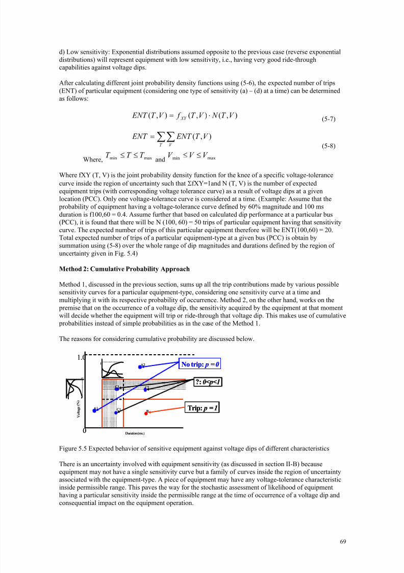
8/20/2019 CIGRE 467 - Economic Framework for Power Quality
http://slidepdf.com/reader/full/cigre-467-economic-framework-for-power-quality 70/151
69
d) Low sensitivity: Exponential distributions assumed opposite to the previous case (reverse exponentialdistributions) will represent equipment with low sensitivity, i.e., having very good ride-throughcapabilities against voltage dips.
After calculating different joint probability density functions using (5-6), the expected number of trips(ENT) of particular equipment (considering one type of sensitivity (a) – (d) at a time) can be determined
as follows:
),(),(),( V T N V T f V T ENT XY ⋅= (5-7)
∑∑=T V
V T ENT ENT ),( (5-8)
Where, maxmin T T T ≤≤ and maxmin V V V ≤≤
Where fXY (T, V) is the joint probability density function for the knee of a specific voltage-tolerancecurve inside the region of uncertainty such that ΣfXY=1and N (T, V) is the number of expectedequipment trips (with corresponding voltage tolerance curve) as a result of voltage dips at a given
location (PCC). Only one voltage-tolerance curve is considered at a time. (Example: Assume that the probability of equipment having a voltage-tolerance curve defined by 60% magnitude and 100 msduration is f100,60 = 0.4. Assume further that based on calculated dip performance at a particular bus(PCC), it is found that there will be N (100, 60) = 50 trips of particular equipment having that sensitivitycurve. The expected number of trips of this particular equipment therefore will be ENT(100,60) = 20.Total expected number of trips of a particular equipment-type at a given bus (PCC) is obtain bysummation using (5-8) over the whole range of dip magnitudes and durations defined by the region ofuncertainty given in Fig. 5.4)
Method 2: Cumulative Probability Approach
Method 1, discussed in the previous section, sums up all the trip contributions made by various possiblesensitivity curves for a particular equipment-type, considering one sensitivity curve at a time and
multiplying it with its respective probability of occurrence. Method 2, on the other hand, works on the premise that on the occurrence of a voltage dip, the sensitivity acquired by the equipment at that momentwill decide whether the equipment will trip or ride-through that voltage dip. This makes use of cumulative
probabilities instead of simple probabilities as in the case of the Method 1.
The reasons for considering cumulative probability are discussed below.
Figure 5.5 Expected behavior of sensitive equipment against voltage dips of different characteristics
There is an uncertainty involved with equipment sensitivity (as discussed in section II-B) becauseequipment may not have a single sensitivity curve but a family of curves inside the region of uncertaintyassociated with the equipment-type. A piece of equipment may have any voltage-tolerance characteristicinside permissible range. This paves the way for the stochastic assessment of likelihood of equipmenthaving a particular sensitivity inside the permissible range at the time of occurrence of a voltage dip and
consequential impact on the equipment operation.
0 Duration (ms.)
V o l t a g e ( % )
1.0
01
1 No trip: p = 0
Trip: p = 1
?: 0<p<1
A2
A1B
C2
C1
C3
0 Duration (ms.)
V o l t a g e ( % )
1.0
01
11 No trip: p = 0
Trip: p = 1
?: 0<p<1
A2
A1B
C2
C1
C3

8/20/2019 CIGRE 467 - Economic Framework for Power Quality
http://slidepdf.com/reader/full/cigre-467-economic-framework-for-power-quality 71/151
70
Let us consider six different voltage-dip events namely, A1, A2, B, C1, C2, and C3 on the voltage-dipchart as depicted in Fig. 5.5. It is obvious from the figure that voltage dips A1 and A2 will never causeany malfunction or trip of the equipment, and therefore the probability of equipment trip is zero.Similarly, voltage dip event B will certainly cause the tripping of the equipment and hence the probabilityof the equipment trip is unity. However, the behavior of the equipment for voltage dips C1-C3 willdepend on the actual sensitivity characteristics of the equipment at the time of these voltage dips. It
implies that there is a certain probability of equipment either surviving these voltage dips or trippingwhen exposed to them. In the case of voltage dip C1, any sensitivity characteristics occurring on the leftof voltage dip C1 will result in equipment trips. Therefore, one has to consider the probability of all thesesensitivity characteristics. This can be taken care of by considering the cumulative probability in such away that its value increases gradually from zero (for the left-most characteristic, i.e., left hand side thicksolid line) to one (corresponding to the right-most characteristic, i.e., right hand side thick solid line).Similarly, all the sensitivity characteristics occurring above the voltage dip C2 will lead to tripping of theequipment, and thus, one has to consider cumulative probability (instead of probability) of occurrence ofthese characteristics such that its value increases from zero (corresponding to top-most characteristic) tounity (corresponding to bottom-most characteristic). In the case of voltage dip C3, all the characteristicsfalling on the left, and above C3 will cause the tripping of the equipment.
Having in mind this discussion, the variation in equipment sensitivity can be represented in terms of uni-
variate random variable (T) in sub-region A, uni-variate random variable (V) in sub-region B, and bivariate random variable (T, V) in sub-region C (see Fig. 5.4) where T and V are assumed to be twostatistically independent discrete random variables. T is the voltage duration-threshold varying betweenTmin and Tmax (determined by the protection settings) and V is the voltage magnitude-threshold varying
between Vmin and Vmax. Therefore, if pX(T) and pY(V) are the probability distribution functions forrandom variable T and V, respectively, then the joint probability distribution function for the bivariaterandom variable (T, V) in sub-region C is given by Bayes rule [156] as follows:
pXY (T, V) = pX(T) pY(V) (5-9)
maxmin T T T ≤≤, maxmin V V V ≤≤
The general trend of sensitivity (e.g. high, moderate, uniform, or good ride-through) of a particularequipment or equipment type can be represented by assuming various types of probability densityfunctions [155] in the sub-regions of uncertainty for one/two random variable(s), i.e., voltage threshold Vand/or duration threshold T as discussed in Method 1. For example, two types of sensitive behavior— highly sensitive and moderately sensitive—are considered in this study with the help of exponential andnormal probability density function, respectively, as depicted in Fig. 5.5.
After calculating probability distribution functions as discussed above, the expected number of equipmenttrips, considering one type of equipment sensitivity at a time, can be determined as follows:
Total equipment trips =∑∑ ⋅T V
XY V T N V T p ),(),( (5-10)
Where ( )V T p XY , is the trip probability of the equipment as defined in (5-9) against the voltage dipswith dip magnitude V and dip duration T, and N (T, V) is the number of such voltage dips expected at thespecified site over specified period of time.
By comparing equations (5-7) and (5-8) with equation (5-10), it is to be noticed that both formulationslook almost identical, but equation (5-7) and (5-8) uses probability density function fXY (T, V), whereasequation (5-10) uses probability distribution function pXY (T, V). Similarly, N(T,V) in equation (5-7)stands for the number of expected equipment trips (with corresponding voltage tolerance curve) as aresult of voltage dips at a given location (PCC), whereas in equation 10, N(T,V) represents the number ofvoltage dips expected (with dip magnitude V and dip duration T) at the specified site over a specified
period of time.
In the absence of any proper information about the type and the nature of operation of the sensitivecustomers connected at the selected network buses, several assumptions can be made. The buses can beranked in the decreasing order of their total connected load and then classified into several different

8/20/2019 CIGRE 467 - Economic Framework for Power Quality
http://slidepdf.com/reader/full/cigre-467-economic-framework-for-power-quality 72/151
71
groups, e.g., Group-I consisting of buses with high loads (>2MW); Group-II consisting of buses withmedium loads (between 1MW and 2MW); and Group-III consisting of buses with loads up to 1 MW.Then, the distribution of total connected load at respective buses among different categories of customersand the corresponding cost per dip can be assumed, e.g., for Group-I buses, 70% of the total loadconnected can be assumed to be large customer loads that run continuous automated industrial processeslike chip-manufacturing plants etc. and remaining 30% comprised of general industrial loads. Group-II
buses mainly supply general industrial loads (70%), some large user load, representing steel plants, packaging plants, bottling plants, dairies, etc. (20%), and a small amount (10%) of commercial load out ofwhich 5% represent large users (e.g., banks), who report huge financial losses due to voltage dips. ForGroup-III buses, it can be assumed that 50% of the total load connected is residential load whose financiallosses due to voltage dips are generally small, and therefore they were not counted in the economicassessment of the total incurred costs. Further, 20% of the connected load comprised of the industrialload, whereas the remaining 30% is commercial load, out of which 5% represent large users (e.g., banks)who report huge financial losses due to voltage dips, etc. To improve further the accuracy of theeconomic assessment, the general trends of various customer types are also considered (see Table 5.1).
The total number of process trips after comparing their sensitivities against voltage dips experienced at aspecific location was therefore multiplied by a suitable correction factor to get the actual number of
process trips attributed to each customer category at a given bus over a year. For example, the commercial
establishments generally remain closed at least for one day in a week—either on Sundays or on Fridaysand are open only for 10 hours a day, from 10 a.m. to 8 p.m. Therefore, a correction factor of [(365-52)/365*10/24]= 0.3573 is used to get actual number of process trips affecting commercial activities(i.e., a voltage dip occurrence when the commercial establishment is closed is not going to disrupt any
process). Similarly, to prevent frequent process disruption and consequential huge financial losses, largeindustries (like chip-manufacturing companies or financial organizations) generally install mitigationdevices (e.g., UPS etc.), which provide ride-through for over 95% of the voltage dips. Therefore, onlyabout 5% of the total voltage dips per year at such customer’s location will still be able to disrupt their
processes.
Finally, the upper limit of maximum one trip per day is enforced on the actual number of process tripsattributed to a particular customer type (i.e. maximum number of process trips per year experienced by acustomer type is 365), whereas the initial assumption was that each trip causes 24 hours of disruption of a
production process.
Table 5.1: Consideration of customer activitiesCustomer type Working trend of customer Correction
factorResidential - -Commercial • One day off per week
• 10 hr/day N = NT*0.3573
Industrial • Two days off• 8 hr/day
N = NT*0.2384
Large users Continuous processInstalled mitigation devicescorrect 95% of PQdisturbances.
N = NT*0.05
(NT – Total number of process trips at the customer site before correction N – Actual number of process trips at the customer site before correction)
After the above-mentioned corrections for the process trips and cost criteria, total voltage dip costs for thesystem considering processes with different sensitive equipment can be calculated.
5.3. End-Use PQ Solutions
A wide range of technologies are available for the mitigation of PQ phenomena. The most common
power quality mitigating technologies in use today are chemical-battery-based uninterruptible power

8/20/2019 CIGRE 467 - Economic Framework for Power Quality
http://slidepdf.com/reader/full/cigre-467-economic-framework-for-power-quality 73/151
72
supplies (UPSs) and transient voltage surge suppression (TVSS), but a great many other types exist andare widely used today.
Uninterruptible Power Supplies
Uninterruptible power supplies (UPS) contain stored energy (usually in the form of conventional
chemical batteries) that can provide replacement power in the event that utility power is interrupted.Some newer UPS topologies use alternative energy storage such as flywheels, ultracapacitors, oradvanced chemical batteries. The annual U.S. market for small (<100 kVA) UPSs is generally estimatedat about $2 billion per year, and growing. There are basically three different types of devices that arecommonly referred to as UPSs: offline (standby), line-interactive, and online. Figure 5.6 provides aschematic view of these three common UPS topologies.
Figure 5.6 The three principal UPS topologies5
1. Offline or Standby UPS
This UPS topology refers to a supply where, under normal circumstances, power is derived directly from
the utility without conditioning. When utility power fails, a battery-powered inverter turns on andsupplies power. The batteries are then charged when utility power is again available.
The pricing on this type of UPS is generally less than other topologies. Disadvantages include theswitchover time—the time required for the inverter to come online. This time can vary from one model ofstandby UPS to another. Because loads are normally connected directly to utility power, this type of UPS
provides relatively poor protection from line noise, surges, frequency variations, and brownouts.
2. Line-Interactive UPS
This form of UPS conditions utility power by employing a ferroresonant transformer. It is thistransformer that acts as an automatic voltage regulator (AVR) standing between the AC input and ACoutput. The AVR maintains a constant output voltage regardless of input voltage, drawing energy from its
internal battery when utility voltage is interrupted or drops too low.5 PQTN Brief #26: UPS Mitigation of Capacitor-Switching Transients, EPRI, Palo Alto, CA: September 1995, PB-105575.
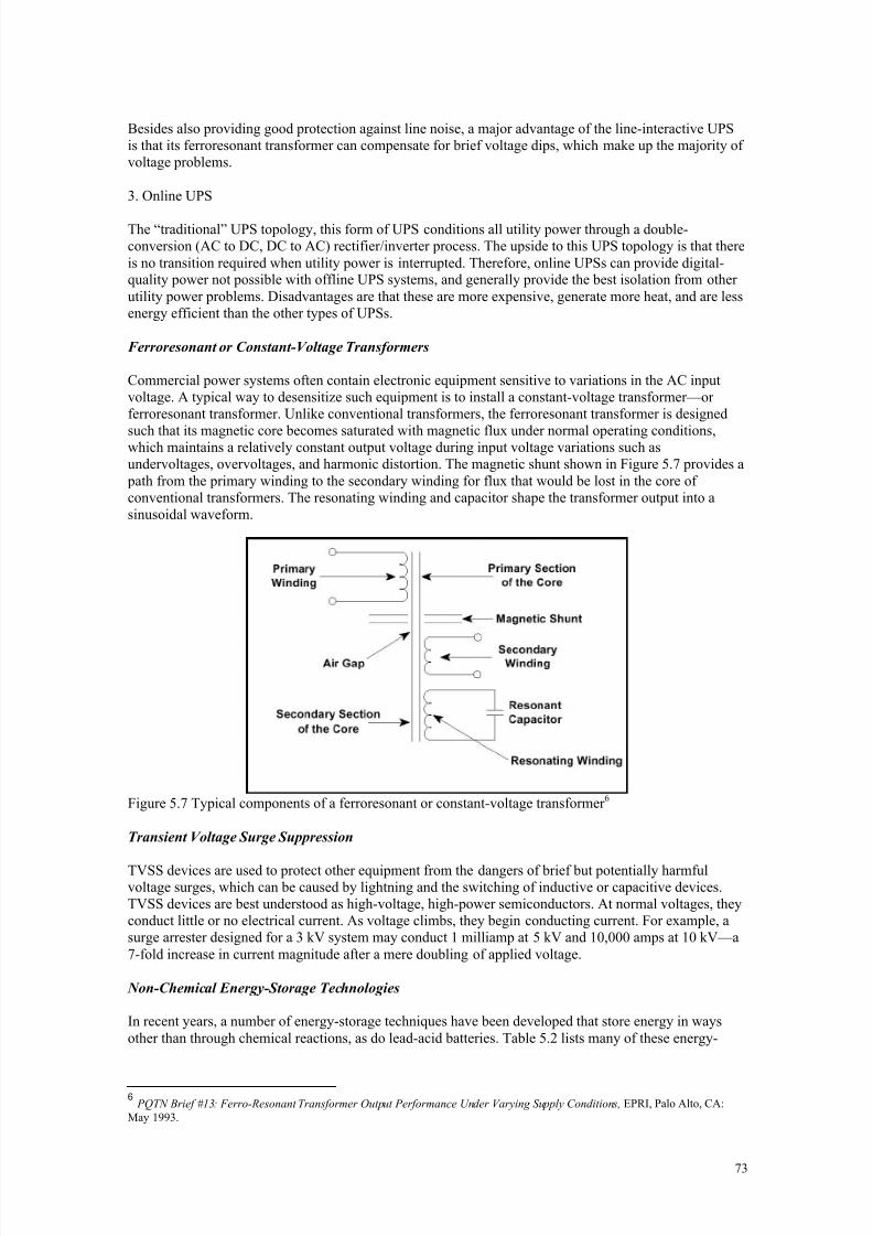
8/20/2019 CIGRE 467 - Economic Framework for Power Quality
http://slidepdf.com/reader/full/cigre-467-economic-framework-for-power-quality 74/151
73
Besides also providing good protection against line noise, a major advantage of the line-interactive UPSis that its ferroresonant transformer can compensate for brief voltage dips, which make up the majority ofvoltage problems.
3. Online UPS
The “traditional” UPS topology, this form of UPS conditions all utility power through a double-conversion (AC to DC, DC to AC) rectifier/inverter process. The upside to this UPS topology is that thereis no transition required when utility power is interrupted. Therefore, online UPSs can provide digital-quality power not possible with offline UPS systems, and generally provide the best isolation from otherutility power problems. Disadvantages are that these are more expensive, generate more heat, and are lessenergy efficient than the other types of UPSs.
Ferroresonant or Constant-Voltage Transformers
Commercial power systems often contain electronic equipment sensitive to variations in the AC inputvoltage. A typical way to desensitize such equipment is to install a constant-voltage transformer—orferroresonant transformer. Unlike conventional transformers, the ferroresonant transformer is designed
such that its magnetic core becomes saturated with magnetic flux under normal operating conditions,which maintains a relatively constant output voltage during input voltage variations such asundervoltages, overvoltages, and harmonic distortion. The magnetic shunt shown in Figure 5.7 provides a
path from the primary winding to the secondary winding for flux that would be lost in the core ofconventional transformers. The resonating winding and capacitor shape the transformer output into asinusoidal waveform.
Figure 5.7 Typical components of a ferroresonant or constant-voltage transformer 6
Transient Voltage Surge Suppression
TVSS devices are used to protect other equipment from the dangers of brief but potentially harmfulvoltage surges, which can be caused by lightning and the switching of inductive or capacitive devices.TVSS devices are best understood as high-voltage, high-power semiconductors. At normal voltages, theyconduct little or no electrical current. As voltage climbs, they begin conducting current. For example, asurge arrester designed for a 3 kV system may conduct 1 milliamp at 5 kV and 10,000 amps at 10 kV—a7-fold increase in current magnitude after a mere doubling of applied voltage.
Non-Chemical Energy-Storage Technologies
In recent years, a number of energy-storage techniques have been developed that store energy in waysother than through chemical reactions, as do lead-acid batteries. Table 5.2 lists many of these energy-
6 PQTN Brief #13: Ferro-Resonant Transformer Output Performance Under Varying Supply Conditions, EPRI, Palo Alto, CA:
May 1993.

8/20/2019 CIGRE 467 - Economic Framework for Power Quality
http://slidepdf.com/reader/full/cigre-467-economic-framework-for-power-quality 75/151
74
storage technologies, their general sizing, and ride-through time (at rated load), as well as some of theirmost attractive applications.
Table 5.2 Capabilities of emerging PQ technologies7 Mitigation Device Power Time ApplicationLarge-scale motor generator
sets (500 KVA)
500 KVA
4160/480
12 seconds Service entry units can be
paralleled bearing maintenance.Low-speed flywheel - DCoutput
250 kW500V DC
12 seconds Support for ASDs, UPSs, andcomputer systems and 4-wiresystem plant-wide support forsections of large installation.
Low-speed flywheel - ACoutput
250 kW480 VAC
12 seconds Support for ASDs, UPSs, andcomputer systems and 4-wiresystem plant-wide support forsections of bearing maintenance.
High-speed flywheel - DCoutput
200 kW600V DC
20 seconds Support for ASDs, UPSs, andcomputer systems. No bearingissues.
Rotating voltage restorer 2000 kW
12,470/12,470
3 seconds Service entry for whole plant
protection. Bearing maintenance.Ultracapacitor -DC output
100 kW100 kW600 V DC
10 seconds5 seconds
Support for ASDs, UPS, andcomputers systems.
Fuel cells - AC output 200 kW480 VAC
Continuous – Noshort-term rating
Sections of load that requirescontinuous power.
Micro turbines AC output 35 kVA Continuous – noshort-term rating
Sub-sections of an industrial plant requiring ultimate securityof supply units can be paralleled.Regular maintenance.
Dynamic dip corrector ACoutput
30 kVA 1∅ 300 kVA 3∅
2 seconds in 1minute3 second firstevent
4-wire system critical sub-sections of industrial plant.
PQ 2000 battery UPS - ACoutput
1 MW2 MW4160 VAC
10 seconds10 seconds
Service entry for whole plant protection. Battery life inquestion.
Micro SMES - AC output 1 MVA2 MVA4160/12,470
1 second1 second
Service entry for whole plant protection.
UPS (single conversion)AC output
Fraction kVA1∅ to 1 MVA3∅ 230 / 480V
15 minutes battery10 secondsflywheel
Single loads through to completesystem. Battery life in question.
Table 5.3 Field evaluation and price of emerging technologiesMitigation Device Field Evaluation Price $/KVAWhere Applicable
Large scale motorgenerators (500 KVA)
Product in manufacture 350
Low-speed flywheel -DC output
Successful application atBG&E with UPS
160
Low-speed flywheel -AC output
Successful application 320
High-speed flywheel -DC output
Successful application -17year life predicted
200
Rotating voltage restorer Successful application 250Ultracapacitor - Successful application 200
7 Combined by EPRI PEAC from Myriad Internal and Industry Sources

8/20/2019 CIGRE 467 - Economic Framework for Power Quality
http://slidepdf.com/reader/full/cigre-467-economic-framework-for-power-quality 76/151
75
DC OutputFuel cells - AC output Successful application 400Micro turbines - ACoutput
Successful application
Dynamic dip corrector -AC output
Successful applicationfor both single and 3-
phase
160
PQ 2000 Battery UPS -AC output
Successful application 400
Micro SMES - ACoutput
Successful application 600
UPS single conversion -AC output
Many successfulapplications
300
Rotary UPS
A rotary UPS uses a rotating mass—most often a heavy flywheel or other form of weighted shaft—tohelp stabilize and maintain rotation of an output generation, similar in concept to how a pottery wheelworks. These systems tend to be large and heavy. The rotating mass often shares a shaft with a hot
standby generator that is started the instant that utility power is lost. One example of a rotary UPS is theHolec/HiTec system.8 Other versions of this concept include rotating AC restorers and some forms ofmotor-generator sets.
Flywheel Energy Storage
Flywheels have been in common use for many years, but only recently were they coupled to electronicsfor electrical energy storage and retrieval. Low-speed flywheels (such as Active Power 9) usually containheavy steel flywheels rotating at 10,000 rpm or less when fully charged and can provide a few seconds ofride-through power at rated load. High-speed flywheels (such as Beacon Power 10 or AFS Trinity11) are theemerging high-tech versions, with composite rotors operating at 50,000 to 100,000 rpm when fullycharged.
Superconducting Magnetic Energy Storage (SMES)
In a SMES system (such as American Superconductor 12), energy is stored within a cryogenically cooledsuperconducting magnet that is capable of releasing megawatts of power within a fraction of a cycle toreplace a sudden loss in line power. In standby mode, the current continually circulates. A power supply
provides a small trickle charge to replace the power lost in the non-superconducting part of the circuit.When a voltage disturbance is sensed, the controller directs real and reactive power from the inverter tothe load, while automatically opening the solid-state isolation switch within two milliseconds. When thevoltage across the capacitor bank reaches a pre-set level, the switch closes. This sequence repeats untilnormal voltage from the utility feeder is restored.
Dynamic Voltage Correction or Restoration (DVC, DVR)
Dynamic voltage restorers (such as S&C Purewave13 and SST DySC14) focus on augmenting voltageduring voltage dips by adding missing voltage at critical times. The theory is that because end users suffermany more voltage dips than outages, having a device that mitigates only dips can do so more cost-effectively than conventional technologies.
Ultracapacitors
8 http://www.hitecups.com/, June 7, 2002
9 http://www.activepower.com/10 http://www.beaconpower.com11
http://www.trinityflywheel.com/12 http://www.amsuper.com13 http://www.sandc.com/products/powerquality.asp14 http://www.softswitch.com/dysc.htm

8/20/2019 CIGRE 467 - Economic Framework for Power Quality
http://slidepdf.com/reader/full/cigre-467-economic-framework-for-power-quality 77/151
76
Capacitors store energy in the form of a voltage field created by electric charge on two large and closelyseparated surfaces. Ultracapacitors (such as Maxwell Technologies15) employ materials that allow anextraordinary amount of stored electrical charge (and therefore energy) in a very small space.
Other PQ-Enhancing Technologies
There are a handful of other PQ-enhancing technologies that bear mention.
Transfer Switches
Power transfer switches allow an end user to switch between alternate sources of power, whether they areonsite generation or a second utility distribution feeder. These technologies are generally grouped into“slow” switches (such as ASCO16), which aren’t capable of protecting the load from interruptions, and“fast” switches (such as Mitsubishi17), which attempt to switch quickly enough so that loads are notinterrupted.
Extent of Use of PQ Mitigation Technologies
A number of studies have asked end users what sorts of PQ mitigation technologies they have purchased.
In all cases, the chemical-battery-based UPS has been the dominant player, usually followed by TVSStechnologies. A recent survey conducted by EPRI PEAC Corporation in the California market bears thisout (see Figure 5.8). A conventional UPS is almost universally applied in commercial and industrialsettings. Surge suppression (TVSS) is the second most common, used at roughly 1/3 of all sites.Currently, the use of DG for PQ purposes is quite limited, but as costs for DG technologies drop, the
potential PQ benefits of DG will likely cause them to be more popular.
The rates of use in Figure 5.8 have been generally mirrored in other studies covering both broad andnarrow geographic areas in the United States.
Use of PQ Mitigation Technologies
92%
30%
20%
20%
12%
8%
0% 20% 40% 60% 80% 100%
Battery-based UPS
Surge protection / TVSS
Capacitors
Transfer switches
Generators
Harmonic filters
Percent of Respondents
Figure 5.8 Survey results: Use of PQ mitigation technologies18
The cost-analysis approach proposed in this chapter is intended to facilitate a balancing of the costs ofunmitigated PQ and reliability phenomena with the costs of preventive measures, with the goal ofachieving the highest net present value (NPV) of overall benefits and costs. Although complete
prevention of all business costs due to PQ and reliability phenomena would be a happy outcome for any
15 http://www.maxwell.com/ultracapacitors/index.html16 http://www.asco.com/home.htm17 http://www.meppi.com/eng_analysis.html18
EPRI PEAC Corporation, Unpublished survey, May 2002

8/20/2019 CIGRE 467 - Economic Framework for Power Quality
http://slidepdf.com/reader/full/cigre-467-economic-framework-for-power-quality 78/151
77
end user, it is seldom economically feasible—only a few highly specialized industries commonly take thisapproach, with data centers, financial facilities, and military facilities being perhaps the best known.Facility planners would like to know how the improved reliability translates into more savings (or lessexpenditure). Therefore, QRA methodology incorporates the NPV technique for engineering costanalysis.
There are many benefits for using an NPV approach for evaluating PQ solutions and, from the perspectiveof the authors, no significant detriments. Any element that results in a cost or profit, revenue in-flow orout-flow, can be considered in the NPV analysis. The resulting combination of mitigation techniquesemployed (including the “do nothing” option of no mitigation) can be weighed and the best alternativeselected or at least identified. The key to the success of the NPV approach is that all scenarios be treatedequally, with the same set of costs or benefits used for each scenario.
The number and type of cost and benefit categories that can be considered for inclusion in the NPVanalysis are virtually limitless. Some likely categories of costs that should be considered include:
• Cost in lost productivity etc. of unmitigated PQ events• Capital cost of PQ solutions• Maintenance costs for PQ solutions
Some likely categories of benefits that should be considered include:
• Reduced maintenance costs• Reduced scrap and material replacement costs• Reduced loss of “good will,” contract defaults, etc.
The number of configurations for possible PQ solutions is almost limitless. Table 5.4 illustrates someexamples compiled by EPRI.
Table 5.4 Examples of power quality problems, costs, and solutions in various industriesCustomerSegment
Type ofEquipmentProblem
Type ofPower-LineDisturbance
Solution Cost of PQ Problem Source ofInformation
Losses (Number/Cost)Equip 1987 1989Lamps 33,45
2$8,363
8,5702143
Motor s
83 2
Boards
563 2
Commercial –AmusementPark
Excessivelamps (81,255lamps on site),electric motors(149 motors onsite), computernetwork boards(1,540 boardson site) failures
Transientovervoltagesdue tolightning
InstalledTVSSs onelectrical
panels in 1989
Total installedcost of TVSSs:$0.14 per parkoperating hour
Electr ical
Maintenance
92.33 per
hour
57.45 per
hour
PreventativeMaintenanceSurvey:TransientElectricalVoltage andLightningSuppression forHBJ ParksOrlando, FL
Healthcare –ResearchCentre
Failure of pressuretransducer onautoclave
Transientovervoltage
InstalledTVSS on panel
poweringautoclave
Cost of PressureTransducer replacement:$1,000 + Labor
Utility,HealthcareCustomer, andAutoclaveServiceCompany
Commercial –OfficeBuilding
Failure of faxmachines
Transientovervoltage
Installed point-of-use TVSS
Over $100 repair foreach fax machine
Utility
Healthcare –
Hospital
X-ray tube
failures
Conducted
emissionsinternal to X-
Installed
tunable filtersto dampen
$80,000 for replacement
cost of one X-ray tube
Utility and
HealthcareCustomer

8/20/2019 CIGRE 467 - Economic Framework for Power Quality
http://slidepdf.com/reader/full/cigre-467-economic-framework-for-power-quality 79/151
78
ray equipment emissionsIndustrial –Chemical Plant
Equipmentshutdowns
Power-linedisturbances
Informationnot available
Loss =$1,000,000/minute
Utility
Industrial –Cement Plant
Computer and programmablelogic controller
failures
Voltage dips UPSs, higher-quality relayswith better
ride-through
Loss = $1,000,000/plantshutdown
Utility andIndustrialCustomer
Commercial –OfficeBuilding
Failure of faxmachine powersupplies
Transientovervoltages
Installed point-of-use TVSS
Power Supply Repair:$127Cost of off-site faxing:$25Loss of time due torepair: $250 – Total:$402 per fax machinefailure
Utility andCommercialCustomer
Healthcare –Hospital
Control systemfailures, circuit
board failures
Voltage dipsand transientovervoltages
CustomizedUPS systemfor imagingsystem
Loss: $10,000/hourCost of UPS: $84,500Cost of circuit boardreplacement:
$20,000/board
ProvidingFluoroscopy InThe CCL DuringElectrical Power
Interruptions,BiomedicalInstrumentation& Technology,1995
Commercial –OfficeBuilding
Fluorescentlighting ballastfailures
Transientovervoltages
Correctedgrounding
problem
Loss: $45.00/ballast +cost of electrician toremove and install new
ballast X 80 ballasts:$8,000
Customer –EPRI/PEACStudy
Picture-TubeManufacturer -Industrial
Downtime, lossof productiondue to processinterruption
Voltage dipsandmomentaryinterruptions
Protectingsensitivecontrol circuitsthroughout the
plant
$100,000/momentaryinterruption,$40,000/dip
Customer –EPRI/PEACStudy
ElectronicsParts forAutomotive -Industrial
Downtime, lossof productiondue to processinterruption
Voltage dips MV staticswitch/DVR
$25,000 per processinterruption
Customer –EPRI/PEACStudy
AircraftEngineManufacturer -Industrial
Downtime, lossof productiondue to processinterruption
Voltage dips Dip- proofing/CVTand Coil Lockcircuit forsensitivecontrols
$100,000 per processinterruption
Customer –EPRI/PEACStudy
Paper & Pulp -Industrial Loss of productivity +equipmentdamage +startup time
Voltage dips Dip- proofing/CVTfor sensitivecontrols
$492,750 for 7 processinterruptions in 1996,includes $100,000equipment damage
Customer –EPRI/PEACStudy
Paper & Pulp -Industrial
Turnover losses Voltage dipsandmomentaryinterruptions
Large-scalereactive powercompensation/UPS,CVT/dip-
proofing/co-generation/islanding
Total $2,740,000turnover losses at 8
paper and pulp mill inSouth Africa in one year
Customer –South AfricanPower QualityConference
Fish Product
Factory-Industrial
Downtime due
to computerlosing track of
Wiring/Groun-
ding inside plant
Isolation
transformer
$4000-7500 lost of
production
Paper, PQ’89,
page 90

8/20/2019 CIGRE 467 - Economic Framework for Power Quality
http://slidepdf.com/reader/full/cigre-467-economic-framework-for-power-quality 80/151
79
batch statusSouth AfricaAll CustomerSegment
Impact of PQon all SouthAfricancustomers
Total impact estimatedto be $300 million peryear; largest portionrelated to voltage dips
Detail Studyconducted byESKOM
Electronics
manufacturing- Industrial
Component
damage + lossof production
Voltage dips
andmomentaryinterruptions
$50,000/year for board
replacement and$50,000/year in loss of
productivity
EPRI PQ
Database
SemiconductorFab processing- Industrial
Wafer losses Voltage dipsandmomentaryinterruptions
Holec ride-through Units
Annual wafer losses$3.1 million
From Customer – SiliconSystems Inc.
5.4. Choosing the Optimal PQ Solution
The basic approach for application of the NPV cost analysis method for evaluation of PQ mitigationoptions is straightforward:
1. The annual cost of unmitigated PQ events for a facility is identified through application of themethods detailed in Chapter 4.
2. The capital and, where appropriate, ongoing operations and maintenance costs for different PQmitigation approaches are identified.
3. A duration (t) for the NPV analysis is identified (the authors recommend 10 years, althoughmore or less may be appropriate for specific industries).
4. A discount rate (r) and inflation rate (i) to reflect the time value of money are identified,5. These parameters are combined in the NPV equation provided below for each mitigation
scenario.6. The scenario producing the highest (or least negative) NPV is identified for final analysis and,
one hopes, implementation at the facility.
The costs and benefits associated with the NPV approach are spread over the entire life span of theequipment used. However, there is a time value associated with money. In order to make a decision, it isimportant to alter the values of costs and benefits over the years to reflect at a common point in time. Inalmost all engineering cost analyses, the common point in time is “the present,” i.e., the planning year [3].Present worth analysis is used to determine the present value of future money receipts and disbursements.The following equation (5-11) converts a stream of annual benefits and costs (annuities) to a presentmonetary value reflective of assumptions for rates for inflation, discount, and escalation:
∑+×++
=
×++=
n
t t
t
tctb
ir
eC C CI NPV
0 )]1()1[(
)1()( (5-11)
Where: NPV = Net present value of a series of cost or benefit
components, CtCI = Initial capital investment (usually expressed as a
negative amount)Ctb = Benefit component occurring at the beginning of
time period tCtc = Cost component occurring at beginning of time
period t (usually expressed as a negative amount)n = Number of time periods, usually in yearse = Escalation rate of C (normally same value as
inflation)
r = Discount rate adjusted for inflationi = Inflation rate

8/20/2019 CIGRE 467 - Economic Framework for Power Quality
http://slidepdf.com/reader/full/cigre-467-economic-framework-for-power-quality 81/151
80
NPV can be compared for different PQ mitigation options. In general, the mitigation option with thehighest (or least negative) NPV would be the most beneficial choice.
5.5. Conclusion
This chapter presents a Net Present Value (NPV) approach as recommended for evaluating differentapproaches for mitigation of power quality. Although a 10-year interval for this evaluation isrecommended and used in the examples provided, it will be incumbent upon each enterprise ororganization applying this method to determine what time interval is most appropriate. Regardless,however, the longer the interval, the more factors other than initial capital cost (such as maintenance, etc.)will figure into the economic evaluation—an approach generally encouraged by the authors.

8/20/2019 CIGRE 467 - Economic Framework for Power Quality
http://slidepdf.com/reader/full/cigre-467-economic-framework-for-power-quality 82/151
81
APPENDIX 1
A Common PQ Phenomena
PQ phenomena are well documented elsewhere; the following paragraphs give a brief description of themost economically disruptive phenomena.
A.1 Categories of Power Quality Variations
The recent proliferation of electronic equipment and microprocessor-based controls has caused electricutilities to redefine PQ in terms of the quality of voltage supply rather than availability of power. In thisregard, the Institute of IEEE Std. 1159-1995, Recommended Practice for Monitoring Electric PowerQuality, has defined a set of terminologies and their characteristics to describe the electrical environmentin terms of voltage quality. A description of the PQ categories as defined by IEEE Std.1159-1995 is
provided in the following subsections.
A.1.1 Voltage Dips and Swells
A voltage dip is a short-duration decrease of the RMS voltage lasting from 0.5 cycle to two minutes induration. These events are caused by faults on the power system or by the starting current of a relativelylarge motor or other large load. A voltage swell may accompany a voltage dip. A voltage swell occurswhen a single line-to-ground fault on the system results in a temporary voltage rise on the unfaulted
phases. Removing a large load or adding a large capacitor bank can also cause voltage swells, but theseevents tend to cause longer-duration changes in the voltage magnitude and will usually be classified aslong-duration variations.
A voltage dip is a short-term reduction in voltage. It is specified in terms of duration and magnitude ofretained voltage. Voltage dips are the result of increased voltage drop in the system caused by increased
current flow either as the result of the addition of a large load, for example the starting current of a largemotor, or due to a fault current. Those caused by large loads are generally localized, often within the sameinstallation, while those due to network fault currents can be widely distributed and affect a large numberof consumers. The characteristics of network dips—magnitude and duration—depend many factors,including the voltage level at which the fault is located, the response time of the protective devices, thedegree of network meshing, the number and configuration of transformers, etc. Most fault-induced dipsare caused by single-phase or two-phase (phase-to-phase) faults. Because three-phase faults are lesscommon than single- and two-phase faults, so too are three-phase dips less likely.
Figure A-1 Classification of Voltage Variations
A.1.2 Momentary Voltage Interruption
A voltage interruption is the complete loss of electric voltage. Interruptions can be short-duration (lastingless than 2 minutes) or long-duration. A disconnection of electricity causes an interruption—usually by

8/20/2019 CIGRE 467 - Economic Framework for Power Quality
http://slidepdf.com/reader/full/cigre-467-economic-framework-for-power-quality 83/151
82
the opening of a circuit breaker, line recloser, or fuse. For example, if a tree comes into contact with anoverhead electricity line, a circuit breaker will clear the fault (short circuit) and the customers who receivetheir power from the faulted line will lose power and experience an interruption. The causes ofinterruptions are generally the same as the causes of voltage dips and swells.
Figure A-2 Examples of Voltage Waveforms for Short-Duration Voltage Variations
System Faults
Customers located on a faulted feeder will experience one or more interruptions, depending on the type offault and the reclosing practices of the utility. For a temporary fault, one or two reclosing operations may
be required before normal power is restored. For a permanent fault, a number of reclosing operations(usually no more than three) will occur before the breaker “locks out” because of the permanent faultcondition. In this case, the customers will experience a sustained interruption. Note that the interruptionsassociated with successive operations of the breaker may be of varying duration, depending on relaycharacteristics. This gives the fault multiple opportunities to clear. The multiple operations also givesectionalizers the opportunity to operate. These devices typically open during the dead time after countinga certain number of consecutive incidents of fault current within a short time period. The number of faultcurrents is typically two, although it could be one if the sectionalizer is at the head of an undergroundcable where all faults are assumed to be permanent.
Reclosing practices vary from utility to utility and, perhaps, from circuit to circuit. Feeders that are mostlyunderground will typically not have any reclosing operations because most faults are permanent. Someutilities are experimenting with faster reclosing times (0.3 to 0.5 seconds) for the first reclosing operationto solve residential customer problems with momentary interruptions. (Residential electronic equipmentsuch as clock radios, VCRs, microwaves, and televisions can often ride through 0.5-second interruptions
but cannot ride through longer-duration interruptions.) At medium voltage levels, it usually takes aminimum of 10 to 12 cycles of dead time to ensure that the ionized gases from faults are dispersed.
Customers located on parallel feeders (that is, feeders that are supplied from the same bus as the faultedfeeder) will experience a voltage dip for the duration that the fault remains on the line. On medium-voltage systems, nearly all faults are cleared within one second and can be cleared in as short as threecycles, depending on the relay settings and the magnitude of the fault current. This means that customerson parallel feeders will experience at least one voltage dip lasting from three cycles to approximately onesecond and possibly additional voltage dips if reclosing operations are required. Voltage dips are muchless severe than interruptions, and the duration of interest is only the period of time that the fault is on theline.
If there are more than two feeders supplied from a common distribution bus, voltage dips will occur morefrequently than actual interruptions because a fault on any one feeder will cause voltage dips on all of theother feeders.
Customers fed directly from the high-voltage system (that is, transmission-fed or large industrialcustomers) usually have more than one line supplying the facility, and actual interruptions should be veryinfrequent for these customers. However, these customers will experience voltage dips during faultconditions over a wide range of the transmission system. Voltage dips caused by faults on a high-voltagesystem generally have more consistent characteristics. The faults that originate in the medium- and low-
voltage systems tend to have more variation.
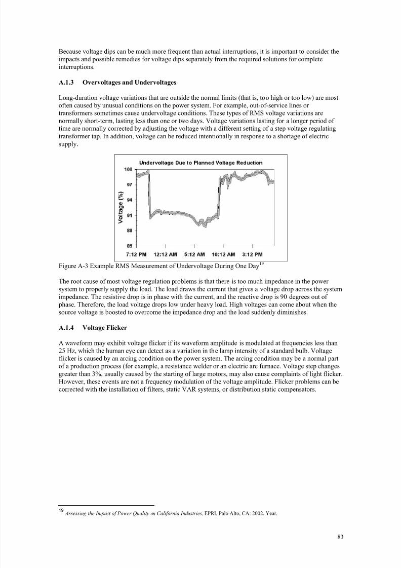
8/20/2019 CIGRE 467 - Economic Framework for Power Quality
http://slidepdf.com/reader/full/cigre-467-economic-framework-for-power-quality 84/151
83
Because voltage dips can be much more frequent than actual interruptions, it is important to consider theimpacts and possible remedies for voltage dips separately from the required solutions for completeinterruptions.
A.1.3 Overvoltages and Undervoltages
Long-duration voltage variations that are outside the normal limits (that is, too high or too low) are mostoften caused by unusual conditions on the power system. For example, out-of-service lines ortransformers sometimes cause undervoltage conditions. These types of RMS voltage variations arenormally short-term, lasting less than one or two days. Voltage variations lasting for a longer period oftime are normally corrected by adjusting the voltage with a different setting of a step voltage regulatingtransformer tap. In addition, voltage can be reduced intentionally in response to a shortage of electricsupply.
Figure A-3 Example RMS Measurement of Undervoltage During One Day19
The root cause of most voltage regulation problems is that there is too much impedance in the powersystem to properly supply the load. The load draws the current that gives a voltage drop across the system
impedance. The resistive drop is in phase with the current, and the reactive drop is 90 degrees out of phase. Therefore, the load voltage drops low under heavy load. High voltages can come about when thesource voltage is boosted to overcome the impedance drop and the load suddenly diminishes.
A.1.4 Voltage Flicker
A waveform may exhibit voltage flicker if its waveform amplitude is modulated at frequencies less than25 Hz, which the human eye can detect as a variation in the lamp intensity of a standard bulb. Voltageflicker is caused by an arcing condition on the power system. The arcing condition may be a normal partof a production process (for example, a resistance welder or an electric arc furnace. Voltage step changesgreater than 3%, usually caused by the starting of large motors, may also cause complaints of light flicker.However, these events are not a frequency modulation of the voltage amplitude. Flicker problems can becorrected with the installation of filters, static VAR systems, or distribution static compensators.
19 Assessing the Impact of Power Quality on California Industries, EPRI, Palo Alto, CA: 2002. Year.

8/20/2019 CIGRE 467 - Economic Framework for Power Quality
http://slidepdf.com/reader/full/cigre-467-economic-framework-for-power-quality 85/151
84
Figure A-4 Example Voltage Waveform Showing Flicker Created by an Arc Furnace20
Voltage Fluctuations
The primary cause of voltage fluctuations is the time variability of the reactive power component offluctuating loads such as, for example, arc furnaces, rolling mill drives, main winders, etc. In general,these loads have a high rate of change of power with respect to the short-circuit capacity at the point ofconnection to the supply.
The magnitude of the fluctuations is usually such that the supply voltage remains within the permittedvoltage tolerance band, but the cyclic nature of the variation, combined with the characteristics of lampsand the response of the human eye and brain, lead to a sensation of flicker. Flicker is an impression ofunsteadiness of illumination that can cause loss of concentration, headaches, and, in some cases, epilepticfits.
A.1.5 Harmonic Distortion
Harmonic distortion is the presence of frequencies at integer multiples of the fundamental systemfrequency, which is 50 Hz in Europe and 60 Hz for the North American power system. Electronic loadsand saturable devices generate harmonic distortion. In commercial facilities, computers, lighting, andelectronic office equipment generate harmonic distortion. In industrial facilities, adjustable-speed drivesand other power electronic loads can generate significant amounts of harmonics.
It is generally safe to assume that the sine wave voltage generated in central power stations is very good.In most areas, the voltage found on transmission systems typically has much less than 1% percentdistortion. However, the distortion may reach 5 to 8% as we move closer to the load. At some loads, thecurrent waveforms will barely resemble a sine wave. Electronic power converters can chop the currentinto a variety of waveforms. Most distortion is periodic, or harmonic. That is, it is nearly the same cycleafter cycle, changing very slowly, if at all. This has given rise to the widespread use of the term“harmonics” to describe perturbations in the waveform. This term must be carefully qualified to makesense.
Figure A-5 Example Voltage Waveform with 3rd Harmonics and 17.42% Total Harmonic Distortion21
20 Assessing the Impact of Power Quality on California Industries, EPRI, Palo Alto, CA: 2002. Year.21
Assessing the Impact of Power Quality on California Industries, EPRI, Palo Alto, CA: 2002. Year.

8/20/2019 CIGRE 467 - Economic Framework for Power Quality
http://slidepdf.com/reader/full/cigre-467-economic-framework-for-power-quality 86/151
85
Solutions to problems caused by harmonic distortion include installing active or passive filters at the loador bus, or taking advantage of transformer connections that enable cancellation of zero-sequencecomponents.
Harmonic frequencies are integral multiples of the fundamental supply frequency. Current harmonics are
generated within the system and in consumer loads by the nonlinear behavior of magnetic materials,rectifiers, and electronic converters. Although harmonic frequencies have always been present in theelectricity system, the increase in the number of equipment using electronic power control in recent yearshas lead to increased levels. Voltage harmonics are created by harmonic currents as they flow throughsystem impedances. Nonlinear loads draw harmonic currents from the supply, thereby producing acorresponding harmonic voltage drop in the impedance of the supply network. As a result, all consumerssee harmonic voltage distortion on the supply voltage. Standards have been introduced to limit theemission of harmonic current by individual items of equipment and by installations in an attempt to limitthe overall level of harmonic distortion on supply networks. Fortunately, the design of networks tends tomitigate some of the effects of harmonic load current—delta transformer windings sink the third andninth harmonic currents emitted by single-phase loads, for example.
Electronic converters also introduce other frequencies into the supply, known as interharmonics. So far,
the magnitude of interharmonic voltages is small.
A.1.6 Unbalance
A three-phase supply system is said to be balanced if the three-phase voltages and currents have the sameamplitude and are separated by 120 degrees with respect to each other. If either of these conditions is notmet, the system is said to be unbalanced. Unbalanced supply voltage usually arises because of unequalloading of the phases at the low voltage level, where most of the loads are single phase. Other causes arethe asymmetry of the distribution system and the connection of large non-three-phase loads, such asrailway connections and arc furnaces.
A.1.7 Voltage Notching
Voltage notching is caused by the commutation of power electronic rectifiers. It is an effect that can raisePQ issues in any facility where solid-state rectifiers (for example, variable-speed drives) are used. Theeffect is caused by the switching action of the drive’s input rectifier. When the drive DC link current iscommutated from one rectifier thyristor to the next, a line-to-line short circuit occurs at the inputterminals to the rectifier. With this disturbance, any given phase voltage waveform will typically containfour notches per cycle caused by a six-pulse electronic rectifier .
Figure A-6 Example Waveform with Notching22
A.1.8 Transient Disturbances
Transient disturbances are caused by the injection of energy by switching or by lightning. The disturbancemay either be unidirectional or oscillatory. Lightning, electrostatic discharge, load switching, or capacitor switching may cause a unidirectional transient. It is characterized by its peak value and rise time. An
22 Assessing the Impact of Power Quality on California Industries, EPRI, Palo Alto, CA: 2002. Year.

8/20/2019 CIGRE 467 - Economic Framework for Power Quality
http://slidepdf.com/reader/full/cigre-467-economic-framework-for-power-quality 87/151
86
oscillatory transient is characterized by its frequency content and may be caused by a switching operationsuch as the energizing of a capacitor bank, distribution line or cable, or interruption of current to aninductive load. The switching of a load may cause high-frequency oscillations with principal frequenciesgreater than 2 kHz. Common solutions to problems caused by transients include the application of surgearresters, passive and active filters, and isolation transformers.
Figure A-7 Example Oscillatory Transient Waveform Caused by Energizing a Capacitor 23
Figure A-8 Example Impulsive Transient Waveform24
23 Assessing the Impact of Power Quality on California Industries, EPRI, Palo Alto, CA: 2002. Year.
24 Assessing the Impact of Power Quality on California Industries, EPRI, Palo Alto, CA: 2002. Year.

8/20/2019 CIGRE 467 - Economic Framework for Power Quality
http://slidepdf.com/reader/full/cigre-467-economic-framework-for-power-quality 88/151
87
Table A-1 Categories of Power Quality Variation—Institute of Electrical and Electronics Engineers(IEEE) 1159-1995
CategoriesSpectralContent
TypicalDuration
TypicalMagnitudes
1.0 Transients1.1 Impulsive
1.1.1 Voltage
1.1.2 Current1.2 Oscillatory1.2.1 Low Frequency1.2.2 Medium Frequency1.2.3 High Frequency
2.0 Short-Duration Variations2.1 Sags
2.1.1 Instantaneous2.1.2 Momentary2.1.3 Temporary
2.2 Swells2.1.1 Instantaneous2.1.2 Momentary2.1.3 Temporary
3.0 Long-Duration Variations3.1 Overvoltages
3.2 Undervoltages4.0 Interruptions4.1 Momentary4.2 Temporary4.3 Long-Term
5.0 Waveform Distortion5.2 Voltage5.3 Current
6.0 Waveform Notching7.0 Flicker8.0 Noise
> 5 kHz
> 5 kHz
< 500 kHz300–2 kHz> 2 kHz
0–100th Harmonic0–100th Harmonic0–200 kHz< 30 Hz0–200 kHz
< 200 µs
< 200 µs
< 30 cycles< 3 cycles< 0.5 cycle
0.5–30 cycles30–120 cycles2 sec–2 min
0.5–30 cycles30–120 cycles2 sec–2 min
> 2 min
> 2 min< 2 sec2 sec–2 min> 2 min
steady-statesteady-statesteady-stateintermittentintermittent
0.1–1.0 pu0.1–1.0 pu0.1–1.0 pu
0.1–1.8 pu0.1–1.8 pu0.1–1.8 pu
0.1–1.2 pu
0.8–1.0 pu000
0–20%0–100%
0.1–7%
Transient disturbances are high-frequency events with durations much less than one cycle of the supply.Causes include switching or lightning strikes on the network and switching of reactive loads on the
consumer’s site or nearby sites. Transients can have magnitudes of several thousand volts and so cancause serious damage to both the installation and the equipment connected to it. Non-damaging transientscan cause severe disruption due to data corruption.
B Response of Sensitive Equipment to PQ Events
B.1 Data Processing and Communications Equipment
This type of equipment operates internally from a low voltage DC supply derived from the AC supply bya rectifier and electronic converter. It is insensitive to moderate levels of harmonic distortion and can bemade immune to most transients, but it is sensitive to voltage dips.
When the supply voltage drops during a dip, the amount of energy delivered to the load is reduced. Theability of the equipment to “ride through” the dip depends on the amount of stored energy available fromthe internal power supply capacitor and the instantaneous energy requirement of the device. A personalcomputer (PC) will have a better ride-through capability while processing than it would have whilewriting to an optical drive, for example.
IT equipment dip performance is described by curves such as the Computer and Business EquipmentManufacturers Association (CBEMA) curve and its more modern Information Technology IndustryCouncil (ITIC) replacement. These curves show the safe operational envelope of the equipment on anominal voltage/time plot. If the duration and retained voltage during a dip lie above the boundary, the
equipment is likely to continue to operate normally.

8/20/2019 CIGRE 467 - Economic Framework for Power Quality
http://slidepdf.com/reader/full/cigre-467-economic-framework-for-power-quality 89/151
88
0
20
40
60
80
10 0
12 0
14 0
16 0
18 0
20 0
0,0001 0,001 0,01 0,1 1 10 100seconds
% n
o m i n a l v o l t a g e
Di p
Interruption
Immunity area
Figure B.1 ITIC Curve
In reality, these curves simply specify typical equipment performance; they do not imply that theequipment will survive the dips that typically occur on the network.
B.2 Variable-Speed Drives
Variable-speed drives (VSDs) use an electronic converter to produce a variable-frequency motor drivevoltage from the fixed supply frequency. Using VSDs is much more energy-efficient than using belts andgearboxes to change speed or using throttle valves to control fluid flows. They are used extensively in
industrial processing, materials handling, and building management.During a dip, the amount of energy supplied by the electrical system is reduced and may be below thatrequired by the process, resulting in loss of control. Because motor-controlled processes rarely operate inisolation, this can result in loss of synchronization with other parts of the process and uncoordinated shutdown.
VSDs usually include a number of measures in order to protect the electronics and the motor fromabnormal conditions, such as undervoltage or loss of a phase voltage, that may trigger shutdown in theevent of a dip.
VSDs draw harmonic currents from the supply. Many drives are designed to minimize or eliminate thesecurrents. VSDs are not affected by normal levels of harmonic distortion.
B.3 Lighting
Any change in supply voltage magnitude may cause a change in the luminous flux or spectral distributionof a light source. Incandescent light sources are particularly sensitive, as the luminous flux isapproximately proportional to the cube of the applied voltage. They are susceptible to “flicker,” which isa subjective visual impression of unsteadiness of a light’s flux, when its luminance or spectral distributionfluctuates with time. The human eye-brain response to variation of luminous flux produces fatigue andloss of concentration for relatively small variations in light intensity at frequencies of about 2 to 20 Hz.

8/20/2019 CIGRE 467 - Economic Framework for Power Quality
http://slidepdf.com/reader/full/cigre-467-economic-framework-for-power-quality 90/151
89
Gas discharge lighting is less sensitive to traditional flicker, partly because it is often electronicallycontrolled, but is affected by a flicker effect due to jitter caused by voltage variation due to interharmonicvoltage distortion. Gas discharge lighting is sensitive to dips: if a dip is deep enough to extinguish thedischarge, a hot lamp may not re-strike when the voltage returns to normal.
B.4 Solenoid-Operated Contactors
Solenoid-operated contactors and relays are used in large numbers in process control systems, and theyare particularly sensitive to voltage dips. “Hardened” devices are available but are relatively rarely used.
C Additional Losses Caused by Poor PQ
Additional losses may be the result of harmonic currents. Load-generated harmonic currents flow ininstallations and in the distributionsystem; they do not transfer energy butdo cause additional loss in cables,transformers, and in motors.
C.1 Cables
In the presence of harmonic currents,the RMS current is higher than thatrequired to energize the load becauseharmonic currents do not transferenergy. This has to be taken intoaccount in sizing conductors.
Zero-sequence harmonics, i.e., those with a harmonic number that is a multiple of three, do not cancel inthe neutral of a three-phase supply. This is important in three-phase cables, which provide supplies tosingle-phase nonlinear equipment where the combined neutral current can exceed the phase currents.
8/20/2019 CIGRE 467 - Economic Framework for Power Quality
http://slidepdf.com/reader/full/cigre-467-economic-framework-for-power-quality 91/151
90
C.2 Transformers
Transformers are affected by harmonic currents. Part of the load loss of a transformer is due to eddycurrent losses in the windings; usually around 5 to 8% of the loss is due to eddy currents and theremainder due to conductor resistance. Eddy current losses are proportional to the square of frequency, soharmonic currents have a serious effect on the heat generated within the transformer, leading to higheroperating temperatures and significant reduction in transformer lifetime.
C.3 Motors
Directly connected motors (i.e., those without a VSD) are affected by harmonic voltage, due to the presence of zero-, positive-, and negative-sequence harmonics. The result is excess heating, increasedmechanical stress, and reduced lifetime.

8/20/2019 CIGRE 467 - Economic Framework for Power Quality
http://slidepdf.com/reader/full/cigre-467-economic-framework-for-power-quality 92/151
91
APPENDIX 2
A Overview of Interruption Cost Calculation
The evaluation of customer outage costs (COC) for a particular service area utilizes three models [36] -System model, which describes the performance of the power system serving the area, Load model, whichdescribes the load connected in the service area at various load points, and Cost model, which representsthe costs due to supply interruptions as a function of interruption duration for a particular customer mix.
The method of Failure Modes and Effect Analysis (FMEA) [70] is normally used for preparing thesystem model. A system model is obtained in terms of a failure rate, average outage duration, and annualoutage time at each load point in the system. Table A-1 illustrates the system model parameters of for two
buses in a general test system.
TABLE A-1: SYSTEM MODEL
Index Bus “n” Bus “k”
λ λ ((f f aauullttss//yyr r )) 0.48 0.46
r (hours) 0.95 0.99
U (hours/ yr) 0.46 0.46
The load model used can be in the form of either average load or actual time-dependant load curves ateach load point. This is used to obtain the annual energy consumed and peak demands for a customer orsector at a given load point. A typical load model is as shown in Table A-2 [42, 71].
TABLE A-2: LOAD MODEL
Sector y E(MWh)
Pmax (MW)
LoadFactor
Residential 8700 2.43 0.409Commercial 14600 3.97 0.420
Industrial 9800 2.00 0.559Total 33100 8.40 0.450
The preparation of the cost model requires the customer survey of the service area to collect perceivedcosts of interruptions of various durations for the customer mix supplied. The cost model is then preparedfor each load point in the area as the normalized costs due to supply interruptions as a function ofinterruption duration. A typical cost model is shown in Table A-3 [42, 71].
TABLE A-3: COST MODEL Duration (r i) C(r i) (£/MWh)
Mom. 0.501 min. 0.52
20 min. 1.341h 2.844h 9.328h 17.2
24h 22.91
Using the above models, the COC at a load point j supplying ny sectors can be calculated as follows:
1
( )ny
j jy j j j
y
COC E C r λ =
= × × ∑ (in £) (A-1)

8/20/2019 CIGRE 467 - Economic Framework for Power Quality
http://slidepdf.com/reader/full/cigre-467-economic-framework-for-power-quality 93/151
92
Where E jy is the annual energy consumed by sector y.
A summation of the COC at all the relevant load points b of a sector gives the annual COC due to supplyinterruptions SCOC as follows:
b
j j bSCOC COC ∈=∑ (in £) (A-2)
B Probabilistic Voltage Dip Costs CalculationThe evaluation of the impact of voltage dips at a particular site in the network involves three basic steps: fault-analysis, voltage dip analysis, and economic analysis. In fault analysis, the method of fault-positions[100] is often used in which various types of faults (symmetrical and asymmetrical) are simulated atnumerous locations throughout the system network, and corresponding expected voltage magnitudes anddurations are determined at various network buses.In a subsequent voltage dip analysis performed at a point of common coupling (PCC), the frequency ofdips of specified dip magnitude and duration over a period of interest is determined by associating it withthe historical fault performance (fault per km per year) of all network buses, overhead lines, and
underground cables. This information is generally available from historic data obtained through long-termmonitoring at respective locations in the network. The corresponding duration of voltage dips depends onfault-clearing times of protective devices used in the power system network.
The final and the most crucial step for the economic assessment of PQ requires the information about theconsequences of expected voltage dips on the performance of industrial processes. This procedurerequires preparing a dip-performance chart for a particular bus in the system and coordination of thecustomer equipment responses with these voltage dips on a single graphic display [72]. The informationabout the equipment sensitivity may be gathered from the equipment manufacturer or by testing. Sensitiveindustrial equipment are classified into various equipment categories based on equipment-types, and thenthe testing is performed on a suitable number of equipment picked randomly from each category.However, even though the equipment may belong to the same equipment category, it might not exhibitthe same sensitivity to voltage dips [73]. This makes it difficult to develop a single standard that defines
the sensitivity of process equipment. In addition to this, it is also possible that a process may be disrupteddue to tripping of individual equipment or it may require the tripping of a group of equipment dependingupon their interconnections. The only way to deal with those uncertainties is to apply probabilisticcalculations relying on expert advice and limited number of field/laboratory tests related toequipment/process sensitivity to voltage dips.The main emphasis of this example, therefore, is to illustrate a probabilistic approach for quantification of
process trips incorporating the uncertainty involved with equipment sensitivity and consequently with the process sensitivity.
C Overview of Equipment SensitivityEquipment sensitivity to voltage dips is usually expressed only in terms of the magnitude and duration ofthe voltage dip. For this purpose, the rectangular voltage-tolerance curve (as shown in Fig. C-1) is used. Itindicates that voltage dips deeper than the specified voltage magnitude threshold (Vmin) and longer thanthe specified duration threshold (Tmax) will cause malfunction (or trip) of the equipment. However, in
practice, some equipment like motor contactors and household electronics items has non-rectangularvoltage-tolerance characteristics [74-77]. Other two parameters, which may be detrimental to sensitivityof some of the industrial equipment such as motor contactors, are point-on-wave of dip initiation and
phase-shift during the dip [75-78].

8/20/2019 CIGRE 467 - Economic Framework for Power Quality
http://slidepdf.com/reader/full/cigre-467-economic-framework-for-power-quality 94/151
93
Fig C-1. Equipment Voltage-Tolerance Curve
Equipment is therefore classified into various categories based on device type, and testing of an adequatenumber of devices representing one equipment category justifies generalization of the acquired results.Because different brands of the same equipment type and even different models of the same brand oftenhave different sensitivities, a typical sensitivity data with appropriate statistical deviation and error
parameters can be determined for the equipment type. The sensitivity information so obtained needs to beupdated continuously as and when more test results become available.
D Uncertainty Involved with Equipment SensitivityIt is found that all the equipment belonging to a particular equipment category do not exhibit samesensitivity against voltage dips [74-79]. However, all equipment types except motor contactors exhibit,more or less, perfect rectangular characteristics. Voltage magnitude-threshold and duration-threshold ofthree equipment types, namely PLCs, ASDs, and PCs, may vary between Vmin and Vmax and between Tmin and Tmax, respectively. The values of these parameters (obtained in tests) are different for differentcategories of equipment. The Vmin and Vmax are 30% and 90%, respectively, for PLCs [78, 80], 46% and63%, respectively, for PCs [79], and 59% and 71%, respectively, for ASDs [86], and corresponding Tmin and Tmax are 20 ms and 400 ms for PLCs, 40 ms and 205 ms for PCs, and 15 ms and 175 ms for ASDs,respectively.
Therefore, the voltage-tolerance curves of these equipment may occur anywhere inside the shaded regionon Voltage dip magnitude v/s duration chart shown in Fig. D-1, such that the knee point of curve alwaysremains inside sub-region C.
Fig. D-1. The region of uncertainty for sensitivity curves of PCs, PLCs, and ASDs
Similarly, the area of uncertainty related to the AC contactors’ sensitivity can be represented by theshaded region shown in Fig. D-2. Their voltage-tolerance curves may appear anywhere in the shadedregion acquiring non-rectangular form for 00 point-on-wave of dip initiation and rectangular form for 900
point-on-wave of dip initiation [ 87-89].

8/20/2019 CIGRE 467 - Economic Framework for Power Quality
http://slidepdf.com/reader/full/cigre-467-economic-framework-for-power-quality 95/151
94
Fig D-2. Probable regions for voltage-tolerance curve of contactors
E Counting of Process TripsThe quantification of expected process trips due to voltage dips over a specified period of time requiresthe knowledge about the mutual connection of sensitive equipment that control the process. Sometimes,tripping of a single equipment may disrupt a complete industrial process, i.e., all the participatingequipment are assumed to be connected in series. On the other hand, the process might be disrupted onlywhen more than one equipment mal-function/trip, i.e., parallel connection of participating equipment. Theoverall probability of process trip can be determined by knowing the probability of trip of individualequipment and their mutual connections. For example, consider a simple process consisting of foursensitive devices having mutual connections as shown in Fig. E-1.
Fig. E-1 Typical connections of sensitive equipment participating in a process
The overall probability of process trip is given by
( ) ( ) ( )4321 1111 p p p p P trip −⋅−⋅−−= (E-1)
Where pi, (i = 1, 2, 3, 4) is the cumulative probability of tripping of ith device. In general, the probabilityof a process trip can be written as
−−= ∏ ∏= =
m
i
n
j
jitrip p P 1 1
,11 (E-2)
Where m is the number of series-connected equipment/equipment groups and n is the number of parallel-
connected equipment in ith equipment group. ji p , is the cumulative probability of tripping of j th
equipment of the ith serially connected equipment group.

8/20/2019 CIGRE 467 - Economic Framework for Power Quality
http://slidepdf.com/reader/full/cigre-467-economic-framework-for-power-quality 96/151
95
Fig. E-2. Expected behavior of sensitive equipment against voltage dips of different
characteristics
A piece of equipment may have any voltage-tolerance characteristic inside permissible range. This pavesway for the stochastic assessment of likelihood of equipment having a particular sensitivity inside the
permissible range at the time of occurrence of a voltage dip and consequential impact on the equipmentoperation. Consider six different voltage dips, namely A1, A2, B, C1, C2, and C3 on the voltage-dip chartas depicted in Fig. E-2. It is obvious from the figure that voltage dips A1 and A2 will not cause anymalfunction or trip of the equipment, and therefore the probability of equipment trip is zero. Similarly,voltage dip B will certainly cause the tripping of the equipment and hence the probability of theequipment trip is unity. However, the behavior of the equipment for voltage dips C1-C3 will depend onthe actual sensitivity characteristics of the equipment at the time of these voltage dips. It implies that thereis a certain probability of equipment either surviving these voltage dips or tripping when exposed to them.
The variation in equipment sensitivity can be represented in terms of uni-variate random variable (T) insub-region A, uni-variate random variable (V) in sub-region B, and bivariate random variable (T, V) insub-region C (see Fig. D-1), where T and V are assumed to be two statistically independent discreterandom variables. T is the voltage duration-threshold varying between Tmin and Tmax (determined by the
protection settings) and V is the voltage magnitude-threshold varying between Vmin and Vmax. Therefore if pX(T) and pY(V) are the probability distribution functions for random variable T and V respectively, andthen the joint probability distribution function for the bivariate random variable (T, V) in sub-region C isgiven by Bayes rule [81] as follows:
pXY (T, V) = pX(T) pY(V); (E-3)
maxmin T T T ≤≤ , maxmin V V V ≤≤
The general trend of sensitivity (e.g. high, moderate, uniform, or good ride-through) of a particularequipment or equipment type can be represented by assuming various types of probability densityfunctions [82] in the sub-regions of uncertainty for one/two random variable(s), i.e., voltage threshold V
and/or duration threshold T.

8/20/2019 CIGRE 467 - Economic Framework for Power Quality
http://slidepdf.com/reader/full/cigre-467-economic-framework-for-power-quality 97/151
96
Fig. E-3. Representation of contactors’ sensitivity with the combinations of uniform and/or normal
probability distributions in various sub-regions of uncertainty
After calculating probability distribution functions as discussed above, the expected number of processtrips, considering one type of equipment sensitivity at a time, can be determined as follows:
Total process trips =∑∑ ⋅T V
trip V T N V T P ),(),( (E-4)
Where ( )V T P trip , is the trip probability of the process as defined in (E-2) against the voltage dips with
dip magnitude V and dip duration T, and N (T, V) is the number of such voltage dips expected at thespecified site over specified period of time.
F Cost AssessmentAs evident from equation (E-4), total number of trips of a given industrial process is dependent on thelocation of the process in the system network and the overall sensitivity of the process against voltagedips. For economic assessment of financial losses due to voltages dips, it is pre-requisite to have theinformation about the type of industrial/commercial process, customer type, mitigation devices installedand the associated damage cost per dip. The total costs incurred due to voltage dips and interruptionsshould be added together in order to come up with total network financial losses for a given networktopology. The implementation aspects of the Bayesian methodology for the assessment of financial lossesdue to voltage dips described above are given in the sequel.
G Numerical Example
The results presented here are based on calculations performed on a generic distribution system (GDS)comprising four 275-kV transmission infeeds, 132-kV and 33-kV sub-transmission networks(predominantly meshed), and 11 kV distribution network (predominantly radial) [83, 99]. The GDSconsists of 295 buses, 296 overhead lines, and underground cables and a large number of switches andcircuit breakers in order to alter the network topology for preventive control and better reliability of thesystem. A large number of transformers having different (Yd, Yy, etc.) winding connections (generally
present in the UK distribution networks) are also modeled.
The base case topology consists of 18 switches in their open position. Additional 40 topologies werederived more or less arbitrarily from the base case topology by opening/closing of some of the open
switches for the purpose of PQ-cost comparison. Some of the actions taken to generate different networktopologies are illustrated in Table G-1. For all these topologies, both interruption and voltage dip costs are

8/20/2019 CIGRE 467 - Economic Framework for Power Quality
http://slidepdf.com/reader/full/cigre-467-economic-framework-for-power-quality 98/151
97
determined. Different network designs/topologies are considered in order to compare and minimize thetotal financial losses in the system.
TABLE G-I: VARIOUS NETWORK TOPOLOGIES CONSIDERED Topology Switching action performed1 Base case
2 All switches closed3 Line 75-231 closed. .40 Lines 3-74, 51-52, 85-87, 75-231, 79-223,
123-129 closed41 Lines 60-64, 61-62, 61-55, 65-55, 66-67,
3-74, 179-26, 25-26, 27-28, 44-222, 36-37, 10-12,51-52, 85-87, 123-129, 215-225 closed; Lines 249-235, 250-236 open.
The input data about the customer interruption costs for different categories of customers is adopted from[42] and shown in Table G-2. For the interruption cost calculation as previously described, the Monte-
Carlo simulation is used. The total system costs due to supply interruptions experienced by customersover a period of one year for the various topologies considered are shown in Table A-VI in the decreasingorder.
TABLE G-2: CUSTOMER INTERRUPTION COSTS (£) VALUES CIC(£) for an interruption duration of :Customer
Type Mom. 1 min. 20 min. 1h 4h 8h 24hRes. - - 0.19 0.70 4.78 - -Com. 11.47 11.74 49.12 106 345 719 1.0kInd. 1.2k 1.5k 2.9k 4.3k 7.6k 12.0k 16.3kL. user 216k 216k 219k 233k 329k 413k 581k
TABLE G-3: TOTAL INTERRUPTION COSTS FOR DIFFERENT TOPOLOGIES Rank
Cost(M£)
Topology No.
RankCost
(M£)Topology
No.1 685.40 2 39 316.17 62 649.67 38 40 311.87 33 630.75 37 41 309.01 1
…
On the basis of the interruption costs only, it is clear from Table G-3 that topology 2 results in hugefinancial losses, whereas the topology 1 is the most economic one. All other topologies result in theinterruption costs in between these two extremes.
For the voltage-dip assessment, the method of fault positions is used considering fault positions onnetwork buses and transmission lines (one fault position per bus and six fault positions per line) [83].Voltage-dip magnitudes at the network buses are calculated for symmetrical and asymmetrical faults atthese fault positions. A conservative approach is adopted for counting process trips due to voltage dips;i.e., the lowest of all phase voltages is considered as the dip magnitude, and it was assumed that thesensitive equipment is connected to the phase experiencing the lowest dip magnitude. The duration ofvoltage dips is determined by the protection fault-clearing time assuming that all faults are cleared by the
primary protection (i.e., 100% reliable primary protection system). The adopted fault rates and durationsare given in [84, 85]. Ten network buses are selected arbitrarily as the buses of interest at which sensitiveindustrial processes are running. Out of these ten buses, the first eight are 11-kV buses, whereas the lasttwo are 33-kV buses.
For the stochastic assessment of process trips taking into account the voltage-dip performance at the site
and the sensitivity of individual equipment participating in the industrial process, six different generic process configurations, as shown in Fig. G-1, comprising of series/parallel connections of four pieces ofcommonly used industrial equipment—PLCs, ASDs, PCs, and AC contactors—are considered. From

8/20/2019 CIGRE 467 - Economic Framework for Power Quality
http://slidepdf.com/reader/full/cigre-467-economic-framework-for-power-quality 99/151
98
these six basic process configurations, 37 distinct processes are derived with two additional assumptions:1) four sensitive devices participating in a process belong to the same equipment-type; 2) all foursensitive devices participating in a process belong to different equipment types. The tripping probabilitiesfor these individual devices are as shown [15].
Fig. G-1: Six typical configurations considered for industrial processes
Because these four sensitive devices are connected in series/parallel combinations, the overall sensitivityof a particular process depends on the equipment type(s), expected range of variation of the sensitivity ofindividual equipment type, and their mutual connections.
In order to get a realistic cost assessment (in the absence of exact information about process distributionamong network buses), it is decided to allocate any ten randomly selected processes (out of 37 available)among ten network buses of interest such that one process is connected to each bus. (Note: Thisassumption allows for the same process to be connected to more than one bus at the same time.) Toachieve this, Monte Carlo simulation is used.
About 10,000 trials were made for the random allocation of processes among ten network buses to get themaximum and minimum range for the system-wide nuisance process trips, once assuming high sensitivityof participating equipment and then assuming moderate sensitivity. After the random allocation of
processes, their nuisance trips are determined and used for the evaluation of financial losses, assumingdifferent categories of customers connected at respective network buses. For the economic assessment ofcustomer losses due to voltage dips, it is assumed (conservatively again) that every nuisance trip of anindustrial process requires 24 hours of restoration time. The damage costs reported by various categoriesof customers for 24 hours long interruption [42] are taken as the damage costs for process trips due tovoltage dips. These costs for different categories of customers are shown in Table G-7.
In the absence of the proper information about the type and the nature of operation of the sensitivecustomers connected at the selected network buses, several assumptions are made in order to account forthose in the most realistic way. The selected ten buses of the network are ranked in the decreasing orderof their total connected load and then classified into three different groups: Group-I consisting of buseswith high loads (>2MW); Group-II consisting of buses with medium loads (between approximately 1MWand 2MW); and Group-III consisting of buses with loads up to approximately 1 MW as shown in Table
G-8. Then, the distribution of the total connected load at respective buses among different categories ofcustomers and the corresponding costs per dip are assumed as shown in Table G-9. For Group-I buses,70% of the total load connected is assumed to be large customer loads, which runs continuous automatedindustrial processes like chip manufacturing plants, glass manufacturing, etc., and remaining 30%comprised of general industrial load. Group-II buses mainly supply general industrial load (70%), somelarge user load, e.g., packaging plants, bottling plants, dairies (20%), and a small amount (10%) ofcommercial load out of which 5% represents users (e.g., banks, data centers) who report huge financiallosses due to voltage dips (see Table G-9). For Group-III buses it was assumed that 50% of the total loadconnected is residential load whose financial losses due to voltage dips are generally small and thereforethey were not counted in the economic assessment of the total incurred costs. Further, 20% of theconnected load comprised of the industrial load whereas the remaining 30% is commercial load out ofwhich 5% represents users who report huge financial losses (as above) due to voltage dips (see Table G-9).
To improve further the accuracy of the economic assessment, the general working trends of variouscustomer types also are considered (see Table G-10). The total number of process trips after comparing
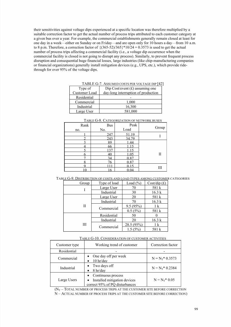
8/20/2019 CIGRE 467 - Economic Framework for Power Quality
http://slidepdf.com/reader/full/cigre-467-economic-framework-for-power-quality 100/151
99
their sensitivities against voltage dips experienced at a specific location was therefore multiplied by asuitable correction factor to get the actual number of process trips attributed to each customer category ata given bus over a year. For example, the commercial establishments generally remain closed at least forone day in a week—either on Sunday or on Friday—and are open only for 10 hours a day—from 10 a.m.to 8 p.m. Therefore, a correction factor of (365-52)/365*10/24 = 0.3573 is used to get the actualnumber of process trips affecting a commercial facility (i.e., a voltage dip occurrence when the
commercial facility is closed is not going to disrupt any process). Similarly, to prevent frequent processdisruption and consequential huge financial losses, large industries (like chip-manufacturing companiesor financial organizations) generally install mitigation devices (e.g., UPS, etc.), which provide ride-through for over 95% of the voltage dips.
TABLE G-7. ASSUMED COSTS PER VOLTAGE DIP [42]Type of
Customer LoadDip Cost/event (£) assuming one
day-long interruption of productionResidential -Commercial 1,000
Industrial 16,300Large User 581,000
TABLE G-8. CATEGORIZATION OF NETWORK BUSES Rank
no.Bus
No.Peak
Load Group
1 247 51.192 243 34.79
I
3 89 1.444 66 1.155 137 1.156 40 1.057 34 0.878 76 0.87
II
9 111 0.15
10 16 0.04
III
TABLE G-9. DISTRIBUTION OF COSTS AND LOAD TYPES AMONG CUSTOMER CATEGORIES Group Type of load Load (%) Cost/dip (£)
Large User 70 581 kI
Industrial 30 16.3 kLarge User 20 581 kIndustrial 70 16.3 k
9.5 (95%) 1 kIICommercial
0.5 (5%) 581 kResidential 50 0Industrial 20 16.3 k
28.5 (95%) 1 kIIICommercial
1.5 (5%) 581 k
TABLE G-10. CONSIDERATION OF CUSTOMER ACTIVITIES
Customer type Working trend of customer Correction factor
Residential - -
Commercial• One day off per week• 10 hr/day
N = NT* 0.3573
Industrial• Two days off• 8 hr/day
N = NT* 0.2384
Large Users• Continuous process• Installed mitigation devices
correct 95% of PQ disturbances
N = NT* 0.05
(NT – TOTAL NUMBER OF PROCESS TRIPS AT THE CUSTOMER SITE BEFORE CORRECTION N – ACTUAL NUMBER OF PROCESS TRIPS AT THE CUSTOMER SITE BEFORE CORRECTION)

8/20/2019 CIGRE 467 - Economic Framework for Power Quality
http://slidepdf.com/reader/full/cigre-467-economic-framework-for-power-quality 101/151
100
Therefore, only about 5% of the total voltage dips per year at such a customer’s location will still be ableto disrupt their processes. Finally, the upper limit of the maximum one trip per day is enforced on theactual number of process trips attributed to a particular customer type (i.e., the maximum number of
process trips per year experienced by a customer type is 365), because the initial assumption was thateach trip causes a 24-hour disruption of a production process.
After the above-mentioned corrections for the process trips and cost criteria, total voltage dip costs for thesystem considering a processes with highly sensitive equipment and then with moderately sensitiveequipment are calculated. The variation in voltage-dip costs for the system obtained in first 12 trials withhighly sensitive and moderately sensitive equipment is shown in Fig. G-3.
The variation in the voltage dip costs for one selected topology (topology 20) is shown in Fig. G-4. It can be seen that the variation in costs due to voltage dips can be very high (between £0.14M and approx.£61M in case of moderately sensitive equipment) depending on the allocation of processes to differentsystem buses. The figure also shows that the sensitivity of the equipment involved in process can increasethe costs up to 50% (e.g. total costs with moderately sensitive equipment for trial 1 are about £61M andwith highly sensitive equipment about £88M).
Finally, the interruption costs and voltage dip costs for 10 different network topologies are addedtogether, and the results are shown in Fig. G-3. It can be seen that the voltage dip costs, when added to theinterruption costs, may alter the total financial losses in the system and in some cases alter the ranking ofthe topologies based initially on interruption costs only. (e.g., topology 20 with dip costs included
becomes “more expensive” than topology 39 for about £3.3M per year). The numerical results areillustrated in Fig. G-5. By comparing the total network losses due to voltage dips with those ofinterruptions it was found that voltage dip costs account for up to about 23% of the total network lossesdue to interruptions.
0
10
20
30
40
50
60
0 1 2 3 4 5 6 7 8 9 10 11
Trial
C o s t ( M £ / y r . )
HS
MS
Fig G-3. Variation in dip costs due to process trips for the whole system (HS – highly sensitive
equipment; MS – medium-sensitive equipment)

8/20/2019 CIGRE 467 - Economic Framework for Power Quality
http://slidepdf.com/reader/full/cigre-467-economic-framework-for-power-quality 102/151
101
0 10 20 30 40 50
60 70 80 90
100
1 5 9 13 17 21 25 29 33 37 41 45 49 53 57 61 65 69 73 77 81 85 89 93 97
Trial
Cost (M£)
HS
MS
Fig. G-4. Variation in total voltage dip cost for network topology
The example illustrated the methodology for comprehensive assessment of financial losses incurred toindividual customers and the whole network over a specified period of time due to two main PQdisturbances: interruptions and voltage dips. The study performed considers modeling of uncertainties
involved with the equipment and process sensitivity and their influence on the quantification of processtrips due to voltage dips. In the absence of the accurate data related to equipment and process sensitivityand corresponding trip/failure costs, which is a common and wide-spread occurrence in this type of study,a probabilistic approach is applied that leads to an estimate of the expected number (range) of processtrips and consequential financial losses. The estimated range of financial losses due to voltage dipscompared to the losses due to outages is in agreement with the reported results based on field surveys.The example further compares total financial losses in the network incurred by interruptions and voltagedips for various network topologies. It is observed that the costs to individual customers and the wholenetwork due to voltage dips alone could be quite substantial (depending on the equipment and processsensitivity) and therefore could have great influence on the total PQ costs.
666.55
472.56 475.9
430.6413.75
398.84365.1
329.69
778.04
736.77
0
100
200
300
400
500
600
700
800
900
2 3 7 3 5 3 2 3 1 2 8 3 6 2 6 3 0 2 4 1 9 2 3 1 3 1 8 1 4 2 7 1 0 4 7 6 1
Topology
C o s t ( M £ / Y r . )
Int. cost
Int. + Min. sag cost
Int. + Max sag cost
Fig. G-5. Comparison of interruption and voltage dip costs for the system: Influence of dip costson total financial losses for the system with various topologies considered

8/20/2019 CIGRE 467 - Economic Framework for Power Quality
http://slidepdf.com/reader/full/cigre-467-economic-framework-for-power-quality 103/151
102
I Typical Loss ValuesTable I-1 Average cost of power interruption. Adopted from [18].
K IEEE 1159 class Average cost(US$/kW)
Cost indexCk
1 Instantaneous 0.078 12 Momentary 0.176 23 Temporary 1.22 154 Sustained 3.63 47
Table I-2 CIC (£) values. Adopted from [42].
CIC (£) for an interruption of durationSector
Momentary 1 min 20 min 1 hour 4 hour 8 hour 24 hour
Residential - - 0.19 0.7 4.78 - -Commercial 11.47 11.47 49.12 106 345 719 1.0k
Industrial 1.2k 1.5k 2.9k 4.3k 7.6k 12.0k 16.3kLarge user 216k 216k 219k 233k 329k 413k 581k
Table I-3 Estimated costs for industrial sectors. Adopted from [14].Voltage Dip Cost (% of total yearly power cost)
Industrial ProcessCategory A Category B Category C
Semiconductor 0 to 2 2 to 10 5 to 6Pharmaceutical 0 to 0.8 1 to 5 2 to 4
Chemical 0 to 1 1 to 3 2 to 4Petrochemical 0 to 1 2 to 5 1.5 to 3.5Manufacturing 0 to 0.2 0 to 1 0.8 to 1
Metallurgy 0 to 0.2 0 to 1.5 1 to 1.5Food 0 to 0.5 0 to 1.5 0 to 2
Table I-4 Direct cost per event per kW. Politecnico di Milano. Adopted from [29].
[€/kW-event] Entire sample (sub-sample)
Median Mean Interval
All sectors 0.8 (1.1) 2.8 (3.3) 0 (0.1) - 30
Per NACE codes
DA – Food products 0.6 5.9 0.2 – 30DB – Textiles 3.2 3.2 3.2DE – Paper 0.8 (0.9) 0.9 (1.0) 0.1 – 2.2
DF – Refined petroleum products 13.3 13.3 13.3DG – Chemicals and man-made fibers 0.6 (0.7) 0.5 (0.7) 0 (0.6) – 0.8DH – Plastic products 1.8 2.2 0.1 – 4.2DI – Glass and ceramic products 0.8 0.9 0.1 – 2.3DJ – Metals products 1.1 (4.9) 3.3 (4.9) 0 (1.1) – 8.7DL – Electrical equipment 9.3 10.6 0.1 – 22.4DM – Auto and auto components 2.9 2.9 0.7 – 5.0
Table I-5 Financial losses due to voltage dips. Adopted from [44].
Industry Typical financial loss per event (€)
Semiconductor production 3,800,000Financial trading 6,000,000 per hour
Computer centre 750,000Telecommunications 30,000 per minute

8/20/2019 CIGRE 467 - Economic Framework for Power Quality
http://slidepdf.com/reader/full/cigre-467-economic-framework-for-power-quality 104/151
103
Steel works 350,000Glass industry 250,000
Table I-6 Financial losses of large commercial and industrial customer for various disturbances. Adopted from [45].
Scenario Financial Losses ($)
4 hour outage without notice 74,8351 hour outage without notice 39,459
1 hour outage with notice 22,973Voltage dip 7,694
Momentary outage 11,027
Table I-7 Impact of voltage dip on industry. Adopted from [49].
Industry Loss per voltage dip ($)
Paper manufacturing 30,000Chemical industry (plastic, glass, etc.) 50,000
Automobile industry 75,000
Equipment manufacturing 100,000Credit card processing 250,000
Semiconductor industry 2.5 million
Table I-8 Summary of all outage cost studies. Adopted from [50].
Study Average cost per hourCost per interrupted kW
or kWhCost per event
Population ResearchSystems
$61,949 for large industrialand commercialAll regions - $59,983
Northwest - $28,609Southwest - $51,908Southeast - $86,477
West - $52,734Midwest - $28,735
ASCO Cellular – $41kTelephone – $72kAirline reservation – $90k
EDF $0.67/kW$8/kWh up to 30MWh$17.4/kWh from 30 to 50MWh
ESOURCE $583k over 800commercial andindustrial customerover 1 year
IEEE 493-1997 Industrial - $6.43/kW +$9.11/kWhCommercial – $21.77/kWh
CEIDS EPRI $7795 for digitalestablishments$14,746 for continuous process manufacturing
Primen Mass Survey $21,688 for 19 businessessurveyed
ICF Consulting 80 to 100 times thecost of retailelectricity
Table I-9 Comparison of interruption costs of industrial customers (in year 2000 US$/kW). Adopted from[51].

8/20/2019 CIGRE 467 - Economic Framework for Power Quality
http://slidepdf.com/reader/full/cigre-467-economic-framework-for-power-quality 105/151
104
Study/Duration 2 second 1 min 20 min 1 hour 2 hour 4 hour 8 hour 24 hour Canada
(small
industrial) 1.07 2.55 3.65 7.71 13.68 28.13 52.06 82.87
England
(industrial) 14.49 15.24 33.62 59.5 - 170.1 283 354.3
USA(industrial)
- - - 9.64 - - - -
Nepal
(industrial - 0.11 0.23 0.42 0.58 1.50 3.00 10.99
Greece
(industrial) 2.10 2.55 7.35 12 16.75 21.80 - 46.86
Taiwan
(high-tech) 37.03 55.15 60.90 87.6 118.1 167.1 242.4 425.2
Table I-10 Voltage-dip sensitivity factors for different industries. Adopted from [32].Category Dip sensitive factor
Semiconductor (SC) 1Computer and peripherals (CP) 0.4Telecommunications (TC), and 0.4
Optoelectronics (OE) 0.6Precision machinery (PM) 0
Biotechnology (BT) 0
Table I-11 Industries surveyed. Adopted from [52].Industry Number of samples Ratio (%)
Food and beverages 49 7.4Textile and apparel 55 8.3
Pulp and paper products 36 5.8Chemical and products 127 19.2Basic/fabricated metal 52 7.9
Other machinery andequipment
49 7.4
Electric and electronicequipment
82 12.4
Electric machinery 53 8.0Audio visual equipment 48 7.3
Motor vehicles 51 7.7Other transport equipment 56 8.5
Table I-12 Interruption cost by duration (unit: Won). Adopted from [52].Interruption cost per average kW ($/kW)
Industry typeBelow 3 seconds Below 1 minutes Below 5 minutes Below 30 minutes
Food and beverages 22.783 44.747 78.020 128.504Textile and apparel 8.421 8.724 9.500 13.935
Pulp and paper products
1.660 1.678 1.781 2.100
Chemical and products
39.805 50.284 52.042 61.505
Basic/Fabricatedmetal
12.886 18.706 33.359 63.288
Other machineryand equipment
11.594 15.950 26.605 59.443
Electric andelectronicequipment
80.335 120.718 174.493 230.076
Electric machinery 7.700 13.634 21.470 45.794Audio visualequipment
9.547 12.709 23.045 53.517

8/20/2019 CIGRE 467 - Economic Framework for Power Quality
http://slidepdf.com/reader/full/cigre-467-economic-framework-for-power-quality 106/151
105
Motor vehicles 23.699 36.683 49.706 83.612Other transport
equipment9.316 12.862 15.782 39.420
Table I-13 Expected losses due to voltage disturbance. Adopted from [53].
IndustryLosses due to voltage disturbance
($/kVA per event)Semiconductors 80 - 120
Glass 10 - 15Automotive 6 - 10
Plastics 4 - 7Textile 3 - 8
Table I-14 Cost per event of interruption
Industry Cost per Event of Interruption
Paper industry $10,000 - $30,000Textile industry $10,000 - $40,000Data processing $10,000 - $40,000Plastic industry $10,000 - $50,000
Semiconductor industry $10,000 - $50,000Automotive manufacturing $15000Source: EPRI – PQ Applications Guide for Architects and Engineers
Table I-15 Average cost of outages. Adopted from [37].
IndustryAverage
cost of downtime ($/hour)
Mobile communications 41,000Telephone ticket sales 72,000
Airline reservation 90,000Credit card operations 2,580,000
Brokerage operations 6,480,000Source: U.S. Department of Energy’s Strategic Plan for Distributed Energy Resources (2000)
Table I-16 Estimated voltage dip costs. Adopted from [37].
Industry Duration Cost/dip
UK steel work 30% for 3.5 cycles £250kUS glass plant Less than 1 second $200kUS computer centre 2 second $600kUS car plant Annual exposure $10MSouth Africa Annual exposure $3B

8/20/2019 CIGRE 467 - Economic Framework for Power Quality
http://slidepdf.com/reader/full/cigre-467-economic-framework-for-power-quality 107/151
106
Fig. I-1 Annual costs due to power quality disturbances for the industrial sector in EU-25 [40]
Fig. I-2 Annual costs due to power quality disturbances for the services sector in EU-25 [40]

8/20/2019 CIGRE 467 - Economic Framework for Power Quality
http://slidepdf.com/reader/full/cigre-467-economic-framework-for-power-quality 108/151
107
Fig. I-3 Annual costs due to voltage dips for five Finnish distribution companies [8]
Fig. I-4 Voltage dip-related cost in different industries. Adopted from [43].
Fig. I-5 Normalized cost per dip as a function of plant power. Adopted from [10]

8/20/2019 CIGRE 467 - Economic Framework for Power Quality
http://slidepdf.com/reader/full/cigre-467-economic-framework-for-power-quality 109/151
108
Fig. I-6 Industry-specific costs of PQ. Adopted from [48].
Fig. I-7 Customer damage functions for different high-tech industry categories. Adopted from [32].
J Typical Financial Loss Values - Summary
TABLE J-1 DIRECT COST PER K W PER EVENT
Section Division ActivitiesFinancial
LossCurrency
DisturbanceType
Small Industrial(Canada)
2.55 US$1-minute power
interruption
Industrial (England) 15.24 US$1-minute power
interruption
Industrial (Nepal) 0.11 US$1-minute power
interruption
Manufacturing General
Industrial (Greece) 2.55 US$ 1-minute powerinterruption

8/20/2019 CIGRE 467 - Economic Framework for Power Quality
http://slidepdf.com/reader/full/cigre-467-economic-framework-for-power-quality 110/151
109
High-tech industry(Taiwan)
55.15 US$1-minute power
interruption
Food products(Italy)
5.9 EuroVery short
interruptionsand voltage dips
Food 8 US$General cost of power quality
Food products and beverages (17, 18)
Food and Beverages(South Korea)
44.75 US$1-minute power
interruption
Textiles (Italy) 3.2 EuroVery short
interruptionsand voltage dips
Textiles 11.7 US$General cost of power quality
Textiles (20)
Textiles (SouthKorea)
8.72 US$1-minute power
interruption
Paper (Italy) 0.9 EuroVery short
interruption andvoltage dips
Paper 1.7 US$General cost of power quality
Paper and paper products (24)
Paper (SouthKorea)
1.67 US$1-minute power
interruption
Coke and refined petroleum products
(26)
Refined petroleum products (Italy)
13.3 EuroVery short
interruptionsand voltage dips
Chemicals andman-made fibers
(Italy)0.5 Euro
Very shortinterruptions
and voltage dips
Chemical 20.6 US$General cost of power quality
Chemical andchemical products
(27)
Chemical and petrochemical(South Korea)
50.28 US$1-minute power
interruption
Plastic products(Italy)
2.2 EuroVery short
interruptionsand voltage dips
Rubber and plastic products (29)
Plastic products 3 US$General cost of power quality
Non-metallicmineral products
(30)
Glass and ceramic products (Italy)
0.9 EuroVery short
interruptionsand voltage dips

8/20/2019 CIGRE 467 - Economic Framework for Power Quality
http://slidepdf.com/reader/full/cigre-467-economic-framework-for-power-quality 111/151
110
Glass products 8 US$General cost of power quality
Primary metal 15.5 US$ General cost of power quality
Basic/ fabricatedMetal (South
Korea)18.71 US$
1 minute powerinterruption
Basic/fabricatedmetals (31, 32)
Metal products(Italy)
3.3 EuroVery short
interruptionsand voltage dips
Electronic 58.3 US$General cost of power quality
Audio and VisualEquipment (South
Korea)12.71 US$
1-minute powerinterruption
Computer,electronic and
optical products(33)
Electrical andElectronic
Equipment (SouthKorea)
120.72 US$1-minute power
interruption
Electric Machinery(South Korea)
13.63 US$1-minute power
interruptionElectrical
equipment (34) Electricalequipment (Italy)
10.6 EuroVery short
interruptions
and voltage dipsMachinery andequipment (35)
Other Machineryand Equipment(South Korea)
15.95 US$1-minute power
interruption
Auto and autocomponents (Italy)
2.9 EuroVery short
interruptionsand voltage dips
Motor vehicles,trailers and semi-
trailers (36) Motor Vehicles(South Korea)
36.68 US$1-minute power
interruption
Other transportequipment (37)
Other TransportEquipment (South
Korea)12.86 US$
1-minute powerinterruption
Transport andstorage
Transportation (55-57)
All transportation 10 US$General cost of power quality
Information andcommunication
Communications(62-66, 86)
Communications 28.6 US$General cost of power quality
Financial andinsuranceactivities
Financial serviceactivities (87)
Business services 3.7 US$General cost of power quality
TABLE J-2 DIRECT COST PER KVA PER EVENT Section Division (NACE code) Activities
FinancialLoss
Currency

8/20/2019 CIGRE 467 - Economic Framework for Power Quality
http://slidepdf.com/reader/full/cigre-467-economic-framework-for-power-quality 112/151
111
Textiles (20) Textile 3 - 8 US$
Rubber and plastic products (29) Plastics 4 - 7 US$
Non-metallic mineral products (30) Glass 10 - 15 US$
Computer, electronic and optical products(336)
Semiconductors 80 - 120 US$
Manufacturing
Motor vehicles, trailers and semi-trailers(36)
Automotive 6 - 10 US$
TABLE J-3 DIRECT COST PER EVENT
Section Division Activities Financial Loss CurrencyDisturbance
type
Large User (UK) 216,000 £
1-minute power
interruption
Large industrial andcommercial (US) 7694 US$ Voltage dip
General Industrial (UK) 1200 £
1-minute power
interruption
Textiles (20) Textile Industry 10,000-40,000 US$Process
interruption
Paper manufacturing (US) 30,000 US$ Voltage dip
Paper and paper products (24) Paper industry 10000 - 30000 US$ ProcessinterruptionChemical and
chemical products(27) Chemical industry (US) 50,000 US$ Voltage dip
Rubber and plastic products (29) Plastic Industry 10,000-50,000 US$
Processinterruption
Glass industry (Europe) 250,000 Euro Voltage dip Non-metallic mineral products (30) Glass plant (US) 200,000 US$ Voltage dip
Steel works (Europe) 350,000 Euro Voltage dipBasic metals (31) Steel works (UK) 250,000 US$ Voltage dip
Semiconductor (Europe) 3,800,000 Euro Voltage dip
Semiconductor (US,Europe and Far East) 2,500,000 US$ Voltage dipComputer, electronic
and optical products(33) Semiconductor 10,000-50,000 US$
Processinterruption
Machinery andequipment (35)
Equipment manufacturing(US) 100,000 US$ Voltage dip
Automobile industry (US) 75,000 US$ Voltage dip
Manufacturing
Motor vehicles,trailers and semi-
trailers (36) Automotive 15,000 US$Process
interruption
Wholesale andretail trade (51-53) Commercial (UK) 11.7 £
1-minute power

8/20/2019 CIGRE 467 - Economic Framework for Power Quality
http://slidepdf.com/reader/full/cigre-467-economic-framework-for-power-quality 113/151
112
interruption
Telecommunications(64)
Telecommunications(Europe) 30,000 Euro Voltage dip
Computer centre (Europe) 750,000 Euro Voltage dip
US computer centre (US) 600,000 US$ Voltage dipInformation andcommunication
Information serviceactivities (66) Data processing 10,000-40,000 US$
Processinterruption
Financial andinsuranceactivities
Activities auxiliary tofinancial services andinsurance activities
(88)Credit card processing
(US) 250,000 US$ Voltage dip
TABLE J-4 A NNUAL COST
Section Division (NACE code) Activities Financial Loss Currency
General Manufacturing 0 - 1 % of total yearly power cost
Food products and beverages (17, 18) Food 0 - 2% of total yearly
power cost
Coke and refined petroleum products(26)
Petrochemical 0 - 5% of total yearly
power cost
Chemical and chemical products (27) Chemical 0 - 4% of total yearly
power cost
Basic pharmaceutical products and pharmaceutical preparations (28)
Pharmaceutical 0 - 5% of total yearly
power cost
Basic metals (31) Metallurgy 0 - 1.5 % of total yearly power cost
Computer, electronic and optical products (33)
Semiconductor 0 - 10% of total yearly
power cost
Manufacturing
Motor vehicles, trailers and semi-trailers (36)
U.S. car plant 10,000,000 US$
Other GeneralSouth Africa
total3,000,000,000 US$
TABLE J-5 COST PER HOUR OF I NTERRUPTION
Section Division (NACE code) Activities Financial Loss Currency
Brokerageoperations
6,480,000 US$
Credit cardoperations
2,580,000 US$Financial and
insurance activities
Activities auxiliary tofinancial services and
insurance activities (88)Financial trading
(Europe)6,000,000 Euro
Information andcommunication
Telecommunications (64)Mobile
communications41,000 US$
Airline reservation 90,000 US$Wholesale and
retail trade
Retail trade, except of motorvehicles and motorcycles
(53)
Telephone ticket
sales 72,000 US$

8/20/2019 CIGRE 467 - Economic Framework for Power Quality
http://slidepdf.com/reader/full/cigre-467-economic-framework-for-power-quality 114/151
113
K Formulae for Computing Harmonic Losses for the Main Electrical
Components
The harmonic losses P T for the transformers (joule and core losses) can be computed as [57-59] :
( ) 1
+3max
1=6.21
1max
1
2
∑∑
=
=
h
hh
mh
co
h
T
h
hh
h
T hV
V P R I P
T
, (K-1)
Where:
I h = current harmonic of order h RT
h = equivalent resistance of the transformer at the harmonic of order h
V h = voltage harmonic of order h
P co
1 = core losses at the fundamental frequency
mT = numerical coefficient
The harmonic losses P M for the induction motors (joule and core losses) can be computed as [57-
59]:
∑∑
=
=
maxh
1h=h6.0
m
1
h1co
hM
maxh
1hh
2
hM
h
Mh
1
V
V P+R
Z
V 3P
M
(K-2)
Where:
Z h = equivalent impedance of the motor at the harmonic of order h
Rh = equivalent resistance of the motor at the harmonic of order hm M = numerical coefficient
Harmonic losses P C for the condensers can be computed as [57-59]:
( ) h2hmaxh
1hhC tgVhC3P δω= ∑
= (K-3)
Where:
ω = angular frequency of system at the fundamentalC = capacitance of the condensertg hδ = loss factor at the harmonic of order h
The harmonic losses P Ca of three-conductors cables (joule and dielectric losses) can be computed as [57-
59]:
( ) ( )∑∑ δω==
hmax
h1=h
2hhCa
hCa
maxh
1hh
2hCa VtghC3+R I3P (K-4)
Where:
RCah = alternating current resistance of one conductor of the cable

8/20/2019 CIGRE 467 - Economic Framework for Power Quality
http://slidepdf.com/reader/full/cigre-467-economic-framework-for-power-quality 115/151
114
C Ca
= capacitance per core;
ω = angular frequency of system at the fundamental.
Other formulas are proposed for a precise evaluation of the equipment loss of life. It is necessary toconsider the operating condition instead of the nominal one.
The operating temperature rise of the hottest point ( OT ∆ ) at operating condition is evaluated by the
following formula.
N
N
O
O T P
P T ∆⋅=∆ (K-5)
Where :
OT ∆ = Expecting temperature rise of the hottest point under operating condition
N T ∆ = Temperature rise of the hottest point under nominal operating condition
O P = Operating power
N P = Nominal power
This formula considers that the equipment is at operating condition since enough time to reach theequilibrium temperature.
The temperature of the hottest point is given by adding the ambient temperature ( AT ) to the temperature
rise.
AOO T T T +∆= (K-6)
And
A N N T T T +∆= (K-7)
The evaluation of the ambient temperature could be problematic. We should consider the cooling systemused. The equipment is inside or outside? Is it in a temperature control environment?
The expecting life under operating power condition ( Ot ) could be evaluated with Arrhenius function [58,
59, 166] knowing the nominal temperature the hottest point and the lifespan of the equipment from themanufacturer.
( )
∆+∆
−⋅= T T T
T
K
E
N O N N et t (K-8)
Where :
N t = Expecting life span under nominal condition
Ot = Expecting life span under operating condition
N T = Expecting temperature of the hottest point under nominal condition (ºK)
N O T T T −=∆ (most of time negative)
The formula presented in chapter 2.2.2.2 will be modified in the following form:

8/20/2019 CIGRE 467 - Economic Framework for Power Quality
http://slidepdf.com/reader/full/cigre-467-economic-framework-for-power-quality 116/151
115
O
O
h
h T P
P T ∆⋅≈∆ (K-9)
( )
∆+∆
−
⋅= hOO
h
T T T
T
K
E
Oh et t (K-10)
Where:
hT ∆ = temperature rise of the hottest point cause by harmonics content
h P = harmonics content
ht = Expecting life span under polluted harmonics condition
There could be more loss of life at operating condition than at rated condition because the life
expectancy Ot will be greater than N t . Utilities could loss more money in reduction of equipment useful
life in harmonics condition when their equipments are operating below their nominal rating.
To do the economic we should find the actual cost for the replacement, in the future, of the equipment.The time used will be modulated by the lifespan of the equipment. This implies the use of the presentvalue formula as presented in chapter 2:
∑++
+×−=
=
n
t t
t
tctb
ir
eC C PV
0 )]1)(1[(
)1()(
(K-11)
This is modified in the following form:
O
O
t
t
E E
ir
eC PV
)]1)(1[(
)1(
++
+×= (K-12)
Where:
E PV = Present value of future equipment replaced in sinusoidal condition
E C = Actual cost for replacing the equipment
Ot = Expecting life span of the actual equipment
This formula gives the actual cost for a future
The same formula is used to calculate the present cost for buying new equipment in ht years representing
the expected lifespan under harmonics condition.
h
h
t
t
E
Eh ir
eC PV
)]1)(1[(
)1(
++
+×= (K-13)
Where:
Eh PV = present cost for buying new equipment in ht years representing the expected lifespan under
harmonic condition
ht = Expecting life span of the actual equipment under harmonics condition
The extra cost for the lifespan reduction due to harmonics will be given by the following formula:
Eh E ELR PV PV C −= (K-14)
This procedure is generic and could be apply for the cost of lifespan reduction for any kind of perturbation.

8/20/2019 CIGRE 467 - Economic Framework for Power Quality
http://slidepdf.com/reader/full/cigre-467-economic-framework-for-power-quality 117/151
116
A global cost evaluation for loss life for distribution system equipment could be perform by orderingequipment in categories representing the kind of equipment and the nominal power in order to reduce theamount of calculation. Time of the day and date of the year could be used to evaluate different load level(operating condition) and fluctuating ambient temperature.
L Methods for Probabilistic EvaluationsThe first step in a probabilistic approach is to recognize that output economical figures to be computedare statistical quantities. In the most general cases, their probability density functions (PDFs) completelydescribe their statistical features. However, for the sake of estimating the economical value of losses and
premature aging due to harmonics, it is adequate referring to the total expected value as:
)(+)(=)( Da E Dw E D E (L-1)
where symbol E(.) indicates the expected value of the quantities already introduced. When estimatingexpected values for a period of time, it is needed to consider their present worth values as:
pw pw pw )(+)(=)( Da E Dw E D E (L-2)
The present worth expected economical value of losses due to harmonics losses, pw)( Dw E , referred to
the whole electrical system life of NT years, is:
( ) ∑∑ −=
T T N
1n1n
n N
1n
pwn
1
Dw E Dw E Dw E
==
pw
)+(
)(=)(
α (L-3)
Where ( ) pwn Dw E is the present worth expected value of the harmonic losses in the nth year, and
n Dw E )( is computed by summing the economical value of harmonic losses of each component in each
jth combination characterized by m j components operating in the same time period ∆T j:
( ) ( )∑=
= jm
1k j ,k j Dw E Dw E . (L-4)
For the g ncombinations taking place in year n, it is:
( ) ∑ ∑ ∑= = =
== n n j g
1 j
g
1 j
m
1k j ,k jn ) Dw( E ) Dw( E Dw E (L-5)
It is clear from relation (L-5) that it is necessary to compute the expected value of harmonic losses for
each component of the system, that is j ,k ) Dw( E . Considering each single electrical component
continuously subject to an hmax harmonics of voltage or current harmonicmaxh2h1h G ,..,G ,G
characterized in the time interval T ∆ by the joint pdf maxh1h G ,..,G f , j ,k ) Dw( E is computed as :
( ) maxh1hG ,..,G0 maxh1h j ,k 0 0 j ,k dG..dG f GG( Dw.. Dw E maxh1h ),..,∫∫ ∫ ∞∞ ∞= (L-6)
with

8/20/2019 CIGRE 467 - Economic Framework for Power Quality
http://slidepdf.com/reader/full/cigre-467-economic-framework-for-power-quality 118/151
117
( T )G ,..,G( P KwG ,..,G Dw Dw maxh1h j ,k
maxh1h j ,k j ,k ∆== (L-7)
For the most common components of industrial energy systems, the harmonic losses
)G ,..,G( P maxh1h
j ,k in (L-7) can be obtained by summing up the losses due to each harmonic so that
the integral in (L-6) can be strongly simplified as:
( ) ∑ ∫=
∞=maxh
1hh
h0 G
h j ,k dG f G Dw Dw E h)( (L-8)
In spite of the apparent complexity of models from (L-3) to (L-8), it is necessary to evidence that themethods practically require the estimation of losses due to harmonics for each component of the system,
paying attention to preliminarily ascertain definite states of operating conditions.
The computation of losses, )( hG Dw in (L-8), does not present particular difficulties; several studies in
literature addressed this subject for the most common components and equipment like transformers, cableline, capacitors, and so on [89-92]; also the formulas shown in Appendix 2-L are valid.
Main difficulties can arise for deriving in each state the PDFs of voltage and current harmonics. Forexisting systems, this can be obtained both from measurements and from simulations adopting well-stated
probabilistic methods of harmonic analysis [92-98].
The present worth economic value of premature aging in (L-2), pw)( Da E , is evaluated by summing the
present worth expected value of the aging costs of each of the N components of the system:
∑=
= N
1k
pwk
pw ) Da( E ) Da( E (L-9)
Where the value of pwk
) Da( E is calculated starting from the knowledge of the useful lives of the
various components by the relation:
pwk )(-)(=)( s
pwk ns
pwk
C E C E Da E (L-10)
where )( pwk sC E and
pwk )( nsC E are the present worth expected value of the costs for buying the
component during the system life in sinusoidal and non-sinusoidal operating conditions, respectively.
The actualization of the costs can be effected in a similar way considering both the discount rate and thecost variation for buying the component; the expected value of cost to be met for buying each componentat year n in a sinusoidal and non-sinusoidal regime is linked to the expected value of the component lifein these conditions, respectively. To estimate these figures, again the cumulative damage theory can beapplied, as in the case of deterministic methods. In such a case, we have to refer to the expected value ofrelative loss of life in the study period; E[ ∆ R L ] computes as:
∏∫∫∞∞
=n
1i
0 n21
x.. x x
0c L dx
) x ,.., x , x( L
f ...T ] R[ E n21∆ (L-11)

8/20/2019 CIGRE 467 - Economic Framework for Power Quality
http://slidepdf.com/reader/full/cigre-467-economic-framework-for-power-quality 119/151
118
wheren x x x f ..21
is the joint PDF of the n random variables on which the component life L depends. The
successive estimation of the useful life can be carried out, as previously mentioned, by summing theexpected values of the relative losses of life until reaching the unity.
The main critical point of this method is linked to the complexity of computing the N dimensional
integral of (L-11) and, overall, to assign the joint PDF n x x x f ..21 . Indeed, some simplificationsintroduced by life models of actual insulated components can greatly help. First of all, in most cases it isadequate to consider electrothermal stress models. Moreover, it is demonstrated that they can be reducedto an even simpler model like:
)(-B cexp K ' L L pn p0 θ −
= (L-12)
Where L0' is life at nominal sinusoidal voltage and reference temperature; cθ =1/θ 0 - 1/θ is the so-called
conventional thermal stress, θ is absolute temperature, θ 0 is a reference temperature (generally the room
temperature); n p and C are model parameters. In particular, n p is the coefficient related to the effect of the
peak of the distorted voltage waveform on life (thus, the larger this coefficient, the stronger the influenceof peak voltage).
Using model (L-12), the general equation (L-11) becomes:
θ θ
∆θ
d dK ) , K ( L
f T ] R[ E
p K T
pc
D D p
p
K
L ∫∫=
(L-13)
Where θ p K f is the joint PDF of the peak factor K p and of the equipment temperature θ , defined in the
time interval T c, p K
D and Dθ are the variation domains of K p and θ , respectively, and L(K p , θ ) represents
the equipment life model expressed by (L-12).
Equation (L-13) still can present some difficulties in deriving the joint PDF of the random variables K p and θ . This joint PDF is generally not directly available. Even in the case in which the statisticalcharacterization of the variables is known, the computation of (L-13) is not immediate, mainly due to thefact that K p cannot be expressed in closed form as a function of voltage harmonics and fundamentalcomponent (infinite different combinations of harmonic vectors can provide a given value of K p). Then,the application of (L-13) in real cases requires the use of Monte Carlo simulation procedures.
Some simplifications can be pursued only in particular cases:
1. As an example, having the aim to highlight only the influence of voltage and current harmonics on
component life, the voltage and current at fundamental frequency, the ambient temperature and theelements of the system admittance matrices at the fundamental, and at harmonic frequencies can beassumed deterministic quantities. Under this assumption, the voltage harmonics are directly linked to thecurrent harmonics injected by nonlinear loads via the elements of the system harmonic admittance matrix.In such a case, the expected value E[ ∆ R L ] of all the MV/LV power system components are a function ofonly the PDF of the magnitude and phase of the current harmonics injected by nonlinear loads, thusreducing the number of random variables to be accounted for.
2. Further simplifications can be achieved computing the life reduction in the worst condition, i.e., thatoccurring when the peak voltage is the arithmetic sum of the voltage harmonic peaks. Applying thissimplification, there is no need to know the PDF of the phase of harmonic currents injected by thenonlinear loads; moreover, in the presence of only one group of nonlinear loads as the main cause ofharmonic pollution, the useful life can be evaluated also with closed form relations, with the simplified
procedure proposed in [54].

8/20/2019 CIGRE 467 - Economic Framework for Power Quality
http://slidepdf.com/reader/full/cigre-467-economic-framework-for-power-quality 120/151
119
In conclusion, to estimate the economical damage due to harmonic losses for each component of thesystem in the study, the following procedure can be observed.
A) Evaluate the expected value of the operating costs due to harmonic losses E[Dw] as follows:
i. Let n1,...,NT be the years of the system study. Let year n1 be assigned to the annual count NN .ii. Let h1,..., H be the harmonics present in the NN th year. Let harmonic h1 be assigned to the harmoniccount NH .
iii. Evaluate the expected value of the operating cost due to the actual NHth harmonic, [Dw(G NH
)] NN ,computing each integral in (L-8) for known f GNH .
iv. Update the harmonic count NH . If NN > NT, go to step v; otherwise go to step iii.v. Sum the integrals obtained in step iii to estimate the operating costs due to harmonic losses E[Dw] NN
in NN th year.vi. Update the annual count NN . If NN > NT, go to step vii; otherwise go to step ii.
vii. Calculate the expected value of the total operating costs, E[Dw], summing the actualized values ofeach considered year E[Dw] NN .
A flow-chart of this procedure is shown in Fig. L-1.

8/20/2019 CIGRE 467 - Economic Framework for Power Quality
http://slidepdf.com/reader/full/cigre-467-economic-framework-for-power-quality 121/151
120
Start
n1 ... N
h1 ... H
[Dw(G NH
)] N
NH= NH+1
yes
NH > H no
E[Dw] NN
NN= NN+1
NN > NT
yes
no
E[Dw]
Stop
Fig. L-1. Flow-chart of the procedure to evaluate the expected value of the operating costs due to harmonic losses
B) Evaluate the expected value of the aging costs due to harmonic losses E[Da], as follows:
i. Evaluate the expected value of the thermal loss of life E[ ∆ RL] in sinusoidal operating conditions bythe integral in (L-13).
ii. Sum the E[ ∆ RL] coming in succession until their sum reaches the unity, so establishing the i-th yearin which the component must be substituted.
iii. Evaluate the purchase cost of the component at the i-th year, taking into account the cost variation to buy it.

8/20/2019 CIGRE 467 - Economic Framework for Power Quality
http://slidepdf.com/reader/full/cigre-467-economic-framework-for-power-quality 122/151
121
iv. Evaluate the expected value of the aging costs in sinusoidal operating condition, E[Cs], summing the purchase costs obtained in step iii, taking into account the present worth discount rate.
v. Repeat steps i. to iv. in non sinusoidal operating conditions to evaluate E[Cns].vi. Calculate the difference between E[Cns] and E[Cs].
A flow-chart of this procedure is shown in Fig.L-2.

8/20/2019 CIGRE 467 - Economic Framework for Power Quality
http://slidepdf.com/reader/full/cigre-467-economic-framework-for-power-quality 123/151
122
Start
E [∆ R L]
yes
Σ E[ ∆ R L ]=1no
purchase cost of the
component
E[C s ]
Stop
Σ E [∆ R L]
E[ ∆ R L ]ns
es
Σ E [∆ R L]ns=1no
purchase cost of
the component
E[C ns ]
Σ E[ ∆ R L ]ns
E [C ns]- E [C s]
Fig. L-2. Flow-chart of the procedure to evaluate the expected value of the aging costs due to harmonic losses

8/20/2019 CIGRE 467 - Economic Framework for Power Quality
http://slidepdf.com/reader/full/cigre-467-economic-framework-for-power-quality 124/151
123
APPENDIX 3
A Cost Aspects
The economic effect of voltage dips and short supply interruptions may differ depending on the time ofoccurrence related to a specific process [120]. It may be without any difference to a control systemwhether a loss of supply is lasting for 100 ms or for one or more hours; depending on the kind ofmanufacturing process and its vulnerability, regarding the before-mentioned consequences and/or servicecosts for re-establishing a related manufacturing process, one case of data loss may result in efforts of upto several thousands of Euros. Depending on the branch, voltage dips or supply interruptions result intocosts in a range from 10.000,-- € (paper, plastic, glass manufacturing) to 700.000,-- € (semiconductormanufacturing) per event [121].
Mathematical Model [106]
Mathematic modeling of costs of loss caused by supply interruptions and voltage dips can be done by
considering these costs consisting of two components: a fix component, that one independent from theduration of voltage loss/reduction; another component proportionate to the duration of voltageloss/reduction [109], what leads to the related specific costs kA affecting the customers:
P W A k t k k +⋅= (A-1)
Where
Ak specific costs of voltage loss/reduction [€/kW]
W k energy-specific, constant-cost component,
independent from the duration [€/kWh]t duration of supply interruption/voltage dip [h]
P k power-specific costs for voltage dips [€/kW]
Some figures on mean cost componentsBased on study results in different European countries, mean values for related costs/kW have beencalculated [106], resulting into the following mean cost components dependent on the duration of supplyinterruption/voltage dip:
Table A-1 Mean cost componentsDuration
“0” 1 15 1 4 8
min min min h h h
Household 0,11 2,28 8,2 25,4Agriculture 0,006 0,03 0,16 16,8 62 96,2
Commerce 1,59 1,92 3,99 13 46,5 80,1
Costs(meanvalues)[€/kW] Industry 2,6 3,5 8,7 17 49,7 80,3
Applying these values to a diagram and, based on linear interpolation, adding trend lines results into thefollowing functions for the mean values for costs of supply interruptions:

8/20/2019 CIGRE 467 - Economic Framework for Power Quality
http://slidepdf.com/reader/full/cigre-467-economic-framework-for-power-quality 125/151
124
Fig. A-1 - Diagram of mean cost components
While the gradient of the trend lines is characteristic for the specific costs of interruptions, the startingvalues at “0” h give the specific costs for voltage dips (and short interruptions).From the results, the following Table A-2 shows the specific voltage dip costs:
Table A-2 Voltage dip costs Specific voltage dips costs kp
/kW
Household 0,29
Agriculture 0,35 (1,53)
Commerce 2,47
Industry 5,49
Some other results from research in other countries are as follows.
A Norwegian research project [108, 112] was undertaken during 2002, aiming besides others to evaluatecustomers’ costs associated with voltage dips and short supply interruptions. The results showed the
following:
Approximate numbers of occurrence per delivery point:
Short supply interruptions, distribution network 13
Voltage dips, distribution network 13
Voltage dips, regional network 63
Overall customers’ costs:
Associated with voltage dips of 23 – 44 M€/year, considering only business customers and voltage dips
with voltage levels reduced by 50% for a maximum of 1 s.
Associated with short supply interruptions of 80 M€/year, considering only business customers.
0
20
40
60
80
100
0 1 2 3 4 5 6 7 8
Agriculture
Industry
Household
Commercial
y = 12 ,51 x + 1 ,5 3
y = 9 ,72 x + 5,49
y = 9 ,97 x + 2,47
y = 2 ,94 x
€/kW
Duration [h]

8/20/2019 CIGRE 467 - Economic Framework for Power Quality
http://slidepdf.com/reader/full/cigre-467-economic-framework-for-power-quality 126/151
125
The average sum of both being in the order of magnitude of the overall customers’ costs associated withlong supply interruptions: (> 3 min) of ~ 113 M€/year
Average specific interruption costs:
• For voltage dips: € 0,67/kW• For short supply interruptions: € 0,93/kW
Investigations by EdF [113] resulted in specific costs of short supply interruptions < 1 min of 0,76 €/kW,while for such shorter supply interruption the Norwegian study resulted in specific costs of 0,85 – 1,25
€/kW [121].
The following example describes the economic effect of losses of supply in the case of a manufacturer intextile (threads):
Consequences:
• Increased piling up of unsalable bobbins, due to malfunction of the manufacturing process.
• Need for 8 hours time until the entire manufacturing system is regularly working again.• Costs for production loss: € 6.300,--, to be completed by staff costs resulting from staff not being
able to do any work (manufacturing process, telephone, PCs), in the considered case to be calculatedwith € 2.000,--/h.
• Other considerations on remedial measures and cost aspects [114].• On principle, remedial measures can be taken on different supply network voltage levels, within the
customer’s installation as well as on equipment design stage (considering modifications of the supplynetwork (HV, MV) design).
• On an LV level, within the customer’s installation to reduce the effects of voltage dips or shortsupply interruptions, targeted at particularly important devices or processes.
• At design and construction of the (more or less) susceptible device
Voltage dips generally imply a solution that provides some means of supporting voltage, whileinterruptions usually require a source of energy to replace the lacking one from the electricity supplynetwork.
Economic considerations play an important part in balancing the cost of the remedial measures with thegravity of the possible disturbance arising from voltage dips or short supply interruptions.
In HV-/MV-network oriented, voltage dips and short supply interruptions are mainly caused by events inthe MV networks, the related percentage being reported by more than 80%. On the network side, the mosteffective method for reduction of ARCs appears to be increased realization of MV lines as buried cables.According to some scientific investigations, 100% cabling would reduce the number of dips by 67%, butdue to longer durations of loss of supply, the end costs would be reduced only by 1%. Huge financialefforts for reaching comprehensively cabled MV networks would be facing a quite modest success related
to the supply interruption costs.Another option is given by dividing given networks. Dividing a network into two halves results in areduction of voltage dips by 50% each. This measure is followed by a decrease of redundancy, a freedomof switching of network parts, as well as a freedom of power plant use and therefore of security of supply[113]. Based on the measure of dividing a given network, a calculation example may highlight the costrelation for statistically avoiding one voltage dip. The example is based on an MV network with a lengthof 4.539 km, this one supplying 616.000 customers. Measurements conducted in the 30 substations of thisnetwork show a mean value of 21,2 voltage dips per substation and year to be expected and a statisticaloccurrence of 0,14 disturbances per km.
Two-busbar operation enables a reduction of occurring voltage dips to half, i.e., 10,1/substation, year. Forenabling this kind of operation, costs of around 15,5 M€ are to be afforded, for 30 Peterson coils and 8
transformers. By this measure, over the entire MV network, statistically 10,1 x 30 = 318 voltage dips peryear are avoided.

8/20/2019 CIGRE 467 - Economic Framework for Power Quality
http://slidepdf.com/reader/full/cigre-467-economic-framework-for-power-quality 127/151
126
Starting from this point and considering the overall effort of 15,5 M€, the costs for avoiding one voltagedip/year for every customer in the considered MV network would statistically amount to around15.500.000 : 318 = ~ 49.000,-- €. Without considering the costs for the transformers, this cost wouldamount to around € 25.000,--.
Taking into account the overall costs of 15,5 M€ for the statistical avoidance of the reduction of the
expectable number of voltage dips to half, these costs were equal to e.g. providing flywheel energystorage (1 MW, € 50.000,--/piece) for 320 enterprises or of flywheel energy storage for 160 enterprises (8M€) + 1.500 smaller UPS (à € 300,--) during 50 years.
Further options are given by the application of voltage stabilizers (dynamic voltage restorers, DVRs),with or without using energy storage units. These devices, normally expected to support the load for ashort period, using heavy-duty batteries, super capacitors, or other forms of energy storage such as high-speed flywheels, generate the missing part of the supply [105].
For shallow dips, where there is considerable retained voltage, so that energy is still available, but at toolow of a voltage to be useful to the load, there are several established automatic voltage regulatortechnologies (automatic voltage stabilizers) [105]. They rely on generating full voltage from the energystill available at reduced voltage during a dip. Because there is no need for any stored energy mechanism,
these devices can be used for long-duration events.
Attention is to be drawn to the selection of an automatic voltage stabilizer in a way to solve the particular problem without creating additional ones. For example, an inappropriate connection of a ferroresonantstabilizer to the output of an inferior generator aiming at a reduction of voltage variations would result inthe affection by frequency fluctuations of the inferior generator, which would produce an AC voltagechange of 1.5% for each 1% change of frequency.
Opposite to the options for voltage stabilizing at MV network level, a well-proven measure to reduce theeffect of voltage dips or short supply interruptions is the application of a UPS to retain the supply of theconsidered system at least for a time to arrange an orderly shutdown, thereby protecting the data, andtherefore enabling the immediate restart of the process after return of the supply. Such UPSs cover arange from very small home user systems to huge systems for the protection of industrial processes.
UPSs for the home or small commercial applications (for example, for the protection of PCs or smallerservers) cost about € 300,--/piece. When considering cost aspects related to the protection of PCs, smallerEDP systems, for 2003, a number of PC shipments for Western Europe of 31,076,639 units is reported,and for 2004, a number of such shipments of 33,720,772 units was forecasted [105].
For a much larger 230/400 VAC UPS used in a customer’s installation, the following data may serve asan example for the features/costs:
• Max. storable energy: 2,7 MJ• Bridgeable time at 100% loss of supply: 1.4 s at 1.400 kVA, 2,8 s at 800 kVA• Purchase costs 1999: ~ 840.000 USD, operating costs per year: ~ 50.000,-- €• Effect: 126 successful carryovers within 55 months
The effect of application of this UPS is to be evaluated by comparing the overall costs for purchasing andoperation with the costs to be expected due losses resulting from 126 events over the time, i. e.:
Expected costs = # Events x $/Event
Alternatively, a buffering unit with electrolytic capacitor can be applied. Compared with a UPS, bufferingunits are smaller, don’t need any maintenance, and are cheaper. Operating without any battery, bufferingunits cause fewer problems at operation and disposal in general.
DC-UPS or buffering unit should ensure
• Bridging of a voltage dip/supply interruption by delivery of Ersatz-current.• Notifying of the occurrence of a voltage dip/supply interruption to the supplied control unit for
starting data storage for the case that the reserve energy would be used up.

8/20/2019 CIGRE 467 - Economic Framework for Power Quality
http://slidepdf.com/reader/full/cigre-467-economic-framework-for-power-quality 128/151
127
• Device oriented.
It is possible to cope with voltage dips/short supply interruptions by enhancing the immunity of electricalequipment and systems from these phenomena, an option that most economically were to be used atdesigning equipment/systems. Sometimes the replacement of older existing equipment, systems or controlunits, may be the most economic solution.
See Brauner study, typical supply dip characteristic and ITIC curve [115].
Fig. A-2 Typical supply dip characteristic and ITIC curve
As conclusions on PQ solutions cost, it appears as very costly to try to cope with the phenomena ofvoltage dips and short supply interruptions by improving the network performance. Through this type ofsolution, elimination of dips may be recognized as probably impossible. In some special cases, where the
need justifies the expense, it may be possible to arrange for dual supplies that are derived fromsufficiently separated parts of the grid as to be considered independent.
Considering the different options for coping with voltage dips and short supply interruptions, Fig. A-3[105] shows the given cost situations, being characterized by a steady increase of costs when movingfrom equipment through the plant to the infrastructure.
The cheapest solution appears to be consideration of dips and short supply interruptions at equipmentdesign, with small effort per piece to make it resilient to the effects of dips and short interruptions. Inmost cases, some form of mitigation equipment is applied within the customer’s installation, due to thekind of equipment/system to be protected.
Figure A-3 Cost mitigation increases as the power level of the load that must be protected increases

8/20/2019 CIGRE 467 - Economic Framework for Power Quality
http://slidepdf.com/reader/full/cigre-467-economic-framework-for-power-quality 129/151
128
B - Hydro-Quebec-Ireq Report for Economical Aspect of Harmonics on
Distribution and Transmission System
In 1998, Hydro-Quebec finalized a technical and economical study on the impact of voltage and currentharmonics on distribution network. Previous studies have been done earlier at a smaller scale covering
only a few lines. The 1998 study was one of the first to cover an entire distribution network and theresults were published in 1999 [165]. An interesting estimation of worldwide harmonic cost was then presented, based on a gross national product extrapolation of countries.
Systematic methodologies were developed for the study considering the literature and know-how of thattime. Formulas representing every aspect of harmonic losses were analyzed. Those formulas cover
power losses (heating) and equipment loss of life. The study includes analysis of distribution and enduser equipments.
Three level of voltage harmonic were considered corresponding to 50%, 100% and 150% of the planninglevel fixed by IEC 61000-3-6 [130]. This approach gives a good figure of the projected economic lossesin term of harmonic level and the results can be used to evaluate the impact of harmonic emission limitchanges, which is mainly ruled by the network regulator.
B.1 Harmonics Power Losses Evaluation
The evaluation of harmonic losses requires the knowledge of voltage and current harmonic level at PCC.For this reason, a typical Hydro-Québec distribution line was used to evaluate the harmonic current fromthe voltage harmonic planning level of the IEC 61000-3-6 [130]. The harmonics losses of this typical linewere then used to extrapolate the results to Hydro-Québec overall distribution network.
B.2 Harmonics Losses Evaluation
The following table gives the overall evaluation of power losses for the distribution network. Theequipments and lines were considered as loaded at nominal capacity.
Table B.1 - Distribution system power losses produced by harmonics at rated load (kW)Harmonics level of 50%IEC
Harmonics level of 100%IEC
Harmonics level of 150%IEC
LV Line 9109 36424 81957MV Line 6894 27575 62043Transformer 2679 10713 24105Capacitor 141 565 1271Total 18823 75277 169376
A similar evaluation was done for the industrial load, which is presented in the following table.Table B.2 - Industrial power losses produced by harmonics at rated power (kW)
Harmonics level of 50%IEC
Harmonics level of 100%IEC
Harmonics level of 150%IEC
Motors 18286 73145 164575Capacitors 111 443 997
In the following tables, factors were applied to present a more realistic figure for the lines and theequipments loading (Lines = 33.8% ; Transformers = 36.4% ; Capacitors = 97% ; Motors = 36.7%).Those factors were determined by Direction Distribution, Hydro-Québec based upon the 1998 operatingcosts and use factor as a function of the annual fluctuation of network load.
Table B.3 - Estimated distribution system power losses produced by harmonics (kW)Harmonics level of 50%IEC
Harmonics level of 100%IEC
Harmonics level of 150%IEC

8/20/2019 CIGRE 467 - Economic Framework for Power Quality
http://slidepdf.com/reader/full/cigre-467-economic-framework-for-power-quality 130/151
129
LV Line 3078 12311 27701MV Line 2330 9320 20970Transformer 975 3899 8774Capacitor 137 548 1233Total 6491 26078 58678
Table B.4- Estimated industrial power losses produced by harmonics (kW)Harmonics level of 50%IEC
Harmonics level of 100%IEC
Harmonics level of 150%IEC
Motors 6711 26844 60399Capacitors 108 430 967
B.3 Harmonic Losses Cost Evaluation
A cost of 0.085$US for each kWh of energy sold was used to produce the annual cost shown in the nexttable. This rate is based upon the projected production cost of a kWh in a thermal plan for year 2000.
Table B.5- Estimated annual cost for distribution system power losses produced by harmonics (k$US)Harmonics level of 50%IEC
Harmonics level of 100%IEC
Harmonics level of 150%IEC
LV Line 2290 9167 20626MV Line 1733 6940 15614Transformer 726 2903 6533Capacitor 102 408 918Total 4833 19418 43692
Table B.6- Estimated annual cost for industrial power losses produced by harmonics (k$US)Harmonics level of 50%IEC
Harmonics level of 100%IEC
Harmonics level of 150%IEC
Motors 4997 19988 44973Capacitors 80 320 720
B.4 Conclusion
Considering that in 2000 the total annual Hydro-Québec distribution electrical consumption was150TWh, the following table presents the percentage of energy losses caused by harmonics.
Table B.7- Estimated distribution system power losses produced by harmonics in percent of total energyused
Harmonics level of 50%IEC
Harmonics level of 100%IEC
Harmonics level of 150%IEC
LV Line 0.018 0.072 0.162MV Line 0.014 0.054 0.122Transformer 0.006 0.023 0.051Capacitor 0.001 0.003 0.007Total 0.038 0.152 0.343
At the time of the study, the harmonics level of Hydro-Quebec’s distribution network was evaluated atnear the 50% IEC planning level. This represents a 0.038 percent of losses caused by harmonics. Forcomparison, a similar study [166], done over the Greek MV and LV distribution network, gives values inthe range of 0.15% to 0.20%, which is more like a harmonics level of 100% IEC level of the Hydro-Québec study. In Greek publication, simplifications and assumptions were made in order to obtain anover estimation of the economical impact of harmonics in the distribution network. The aim was toconclude that it is useless to put effort in network harmonics improvement. Both results could not bedirectly compared in term of network configuration, equipment characteristics, harmonics level,technique used and assumptions made, but they are quite similar.
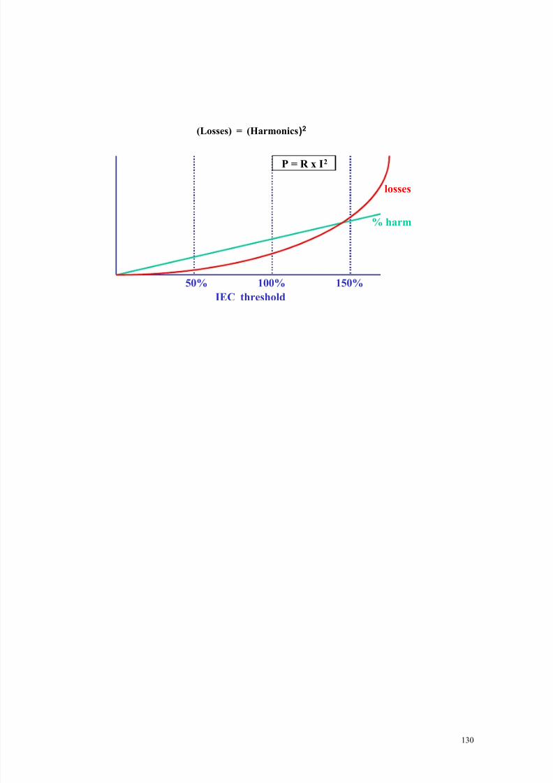
8/20/2019 CIGRE 467 - Economic Framework for Power Quality
http://slidepdf.com/reader/full/cigre-467-economic-framework-for-power-quality 131/151
130
(Losses) = (Harmonics)2
50% 100% 150%
IEC threshold
losses
% harm
P = R x I2

8/20/2019 CIGRE 467 - Economic Framework for Power Quality
http://slidepdf.com/reader/full/cigre-467-economic-framework-for-power-quality 132/151
131
APPENDIX 4
A Structuring the Data Collection ProcessFor the purpose of structuring the data collection process, a proper taxonomy can be useful; in thefollowing the most important items are recalled and described.
Critical sectors
They are in general PQ critical and demonstrate similar PQ sector sensitivity, for which the methodologycan be potentially targeted.
CS1. Industrial sectors type uni-product / uni-process (continuous manufacturing)
1. Food / Beverage (production processing and preserving, NACE25 15)2. Glass, ceramics, cement, lime and stone (NACE 26)
3. Metallurgy (NACE 27)4. Pharmaceutical ( NACE 24.4)5. Plastic and rubber (NACE 25)6. Publishing, printing and reproduction of recorded media (NACE 22)7. Pulp and Paper industry ( NACE 21)8. Refineries, chemical industry (NACE 23.2, 24 except 24.4)9. Semiconductor industry (NACE 32.1)10. Textile (particularly preparation, spinning and manufacture NACE 17.1 and 17.5)11. Wood and wood products (particularly production of sheets, boards and panels NACE 20.2)
CS2. Industrial sectors type multi-product / multi-process
1. Automotive industry (NACE 34)
2. Continuous or highly automated or precision manufacturing – not defined in other sectors -metal products (NACE: 28 fabricate metal products - except structure work 28.1 , 30 - officeequipment, 31- electrical equipment, 32 – except 32.1 – RTV and telephony electronics, 33 –medical equipment)
3. Manufacture of machinery (NACE 29 and 31)
CS3 Services sectors
1. Air transport (NACE2 62)2. Database activities e.g. hosting services (NACE 72.4)3. Financial intermediation (particularly central banking, but also other general transactions, section
J; NACE 65-67)4. Hospitals (NACE 85.1)5. Hotels (NACE 55.1)6. Railways (NACE 60.1)7. Telecommunications (NACE 64.2)
Cost categories
1. Process interruptions2. Process slowdown3. Equipment damage4. Reduced lifetime and mis-operation (postponed costs)5. Reduced energy efficiency - increased energy loss
25 The NACE Code is a pan-European classification system which groups organisations according to their business activities;http://ec.europa.eu/comm/competition/mergers/cases/index/nace_all.html

8/20/2019 CIGRE 467 - Economic Framework for Power Quality
http://slidepdf.com/reader/full/cigre-467-economic-framework-for-power-quality 133/151
132
6. Product quality7. Worker productivity8. Other indirect costs
Cost types - Operating consequences
1. WIP loss, often referred to as production loss or production damage. This category includes this part of labor and material costs which has been inevitably lost. This category has two majorcomponents - labor and material cost.
2. Working capacity loss – basically quantifies efforts to make up this part of production which canstill be repaired or reused – WIP recovery
3. Labor cost resulting from production outage – lost or extra paid4. Other related costs when quantification using above mentioned categories is not easily possible.
These could be a process slow down when it cannot reach its nominal efficiency including process restart cost and additional maintenance costs. These include process and process restartcost.
5. Equipment related costs, including equipment damage and replacement costs, hire of temporaryequipment, and running costs of back up equipment
6. Indirect costs, e.g. consequences of late delivery such as penalties to clients, extra compensation
to personnel, cost of personnel or equipment evacuation, extra insurance cost7. Savings from unused resources (labor, energy, material).
PQ phenomena
1. Voltage dips and short interruptions2. Harmonics (current and voltage)3. Surges and transients4. Flicker5. Unbalance6. Earthing and EMC
Equipment:
as a PQ source and affected by PQ
1. Capacitors2. Contacts and relays3. Electric motors4. Electronic equipment5. Lighting equipment6. Processing equipment7. UPS uninterruptible power supplies8. VSD and other static converters9. Welding and smelting equipment
PQ consequences
1. Circuit breakers (including protective devices) nuisance tripping2. Capacitor damage3. Capacitors – dielectric loss4. Computer lock up5. Computers / other electronics damaged6. Data loss7. Electric shock8. Lights flicker or dim9. Loss of synchronization of processing equipment10. Motors / process equipment - malfunction or damage11. Motors overheating – energy losses
12. Noise interference to telecom lines13. Relays /contactors nuisance tripping

8/20/2019 CIGRE 467 - Economic Framework for Power Quality
http://slidepdf.com/reader/full/cigre-467-economic-framework-for-power-quality 134/151
133
14. Transformers / cables overheating with related energy losses15. Premature ageing and loss of reliability of electrical equipment16. Overheating of neutral conductor in lines and transformers and related problems (e.g. transient
overvoltage, tripping of RCDs, losses)
Solutions
1. Equipment immunity2. Backup generator3. Dynamic voltage restorers4. Harmonic filter5. Isolation transformers6. Line conditioners or active filters7. Multiple independent feeder8. Oversizing equipment9. Shielding and grounding10. Site generation capable of substituting supply11. Static transfer switches12. Static VAR compensator
13. Surge protectors on key pieces of equipment14. Uninterruptible power supply (UPS) devices15. Voltage stabilizers
B Executing Data Collection Process – End User Perspective
With reference to the Model A presented in Chapter 4, the following step-by-step procedure can berecommended to estimate the process interruption cost, PIC:
• Step 1: Based on the assumptions mentioned above, evaluate the total number of productvariants, the total number of process activities at any given instant and the maximum number of
potential failures among all process activities.
• Step 2: For each product variant, determine the associated progressive cost components fromA1 to A726 for each process activity. Note: If for a particular process activity the maximum numberof failure scenarios is less than the maximum number of failure scenarios in all process activities,then the cost components A2, A3, A4 and A5 associated with failure scenarios assumes zero value.Establish the cost related to component A6, particularly employees tolerance for each failure instanceof process activity. Establish customer satisfaction and reputation retained level for instance of non-delivery of a product variant in time. Finally calculate savings A7 due to failure scenarios.
• Step 3: Prepare a work schedule highlighting the active process activities for a typical day forwhich process interruption cost profile has to be established. This work schedule should include
process activities for various product variants and their simultaneous.
The proposed specification and division of sectors by Taxonomy A may help an end user to focuseconomic data collection on certain aspects.
The proposed methodology suits the collection of cost data in ‘industrial - uni-process’ sectors. Most of processes are organized in a series topology as indicated in the Figure B.1. With reference to Fig.B.1, thestream I is the simple extreme. In such a case, close attention should be paid to the calculation of processinterruption costs as all the processes are closely interdependent. In a ‘Just in time’ scenario, where thereare no buffers in the process, one process failure may stop the whole production line.
These sectors are particularly vulnerable to voltage dips and related process interruptionsFor sectors classified as ‘Industrial - multi-process’, the production process is less often performed incontinuous stream – Figure B.1 – stream VI, as an extreme. In such case one process interruption may not
26 Chapter 4 clause 4.3.2

8/20/2019 CIGRE 467 - Economic Framework for Power Quality
http://slidepdf.com/reader/full/cigre-467-economic-framework-for-power-quality 135/151
134
necessarily stop other processes. The consequences are limited to the critical processes which are neededto make up for lost lead time of the final product. The focus is therefore on extra cost (e.g. bonus extratime labor cost) to recover lost or partly lost WIP (A127).
These sectors are vulnerable to voltage dips but also other phenomena like harmonics and unbalance,transient and surges.
Figure B.1: Six typical configurations considered for industrial processes
In the ‘Services’ sectors it can be difficult to distinguish the root cause of process interruption, particularly in a commercial environment where software, hardware or a PQ issue maybe responsible.
Once the root cause has been attributed to PQ, the consequences could be:
• Loss of transactions in progress requiring data recovery, reprocessing and repeated transmission. Thestandard data collection process described here should be modified either using a mix of A1, A2 andA5 cost components.
• Process restart cost using A4 cost calculation• Other costs, particularly lost revenues (missed opportunities) as result of customer dissatisfaction and
loss of reputation, but also such consequences as penalties and other elements of A5 cost component.• Potential savings from A7 are usually negligible.
The alternative to the procedure described above is to use A3, the process slow down method, to simplycalculate business slow down rate.
In addition, due to lack of clear differentiation whether a process was interrupted or not, all phenomenarelated cost components should be used to check that nothing has been omitted. It also should be checked
whether any items have been double counted, particularly A5 (equipment damage due to processinterruption) and equipment damage due to occurrence of PQ disturbance.
Service sectors are relatively more vulnerable to the consequences of long interruptions but PQ may still be the root cause of substantial economic losses.
C ConclusionsDeregulation and industry restructuring are placing utilities under increasing pressure to both improvecustomer reliability and decrease cost. To remain competitive, it is critical to prioritize maintenance tasksso that the best possible reliability is achieved with increasingly constrained maintenance budgets.
27 Chapter 4, clause 4.3.2
I
II
III
IV
V
VI

8/20/2019 CIGRE 467 - Economic Framework for Power Quality
http://slidepdf.com/reader/full/cigre-467-economic-framework-for-power-quality 136/151
135
The purpose of maintenance is to extend equipment lifetime and/or reduce the probability of failure.Corrective maintenance replaces or repairs failed components, while preventive maintenance is a
proactive effort to improve the condition of an unfailed component that may be deteriorated to somedegree.
Power quality can be surveyed for three major purposes:
1. Technical reasons (which are more important in industrial centers and to facility managers)2. Economic reasons (including all sectors linked with the electrical system)3. Social reasons (in which the governmental system is bound to offer desirable services)
Appropriate quality of electrical energy can greatly reduce expenses arising from losses or systemdisturbances. Improvement of power quality can overcome these problems as well as increase equipmentlongevity and system reliability.
In poor power quality, financial damages imposing upon residential, industrial, and trade consumptionwould be very different. Therefore, it must not be neglected that some huge portion of electrical energy isconsumed in residential utilization. Losses of power, decline in useful life of power system equipment, aswell as non-purchased energies due to power quality deficit are counted as parts of financial damages
imposed upon facility managers. Furthermore, governments fulfill community satisfaction and demandswith legislation for facility managers. All the above-mentioned instances appear as positive pressure in promotion of power quality in a power system.
The scientific response is that they are only due to economic limitations, which of course the alternativeimplication may be suffering from poor initiatives in establishment of state laws in this respect and alsolacking practical scientific capability necessitated in supplying those wants.
In this report, attempts have been made toward implicating economic damages resulting from quality problems encountered with shape of consumption. Requirement investment for power quality promotioncounts as main criteria for comparison.

8/20/2019 CIGRE 467 - Economic Framework for Power Quality
http://slidepdf.com/reader/full/cigre-467-economic-framework-for-power-quality 137/151
136
APPENDIX 5
A Illustrative Case Study
This section illustrates the application of the NPV approach to a hypothetical high-tech facility based onan actual facility. The example considers a semiconductor wafer-fabrication factory located in the UnitedStates. Wafer fabrication requires a high level of power quality and reliability due to the sensitivity of theequipment and process controls and therefore is a strong candidate for applying the NPV analysis.
A.1 Base Case: Facility Data and Base Case Calculations
For purposes of this case study, each process interruption resulting from an unmitigated voltage dip isassumed to cause an overall business loss of $500,000 from various factors, including lost production,extra labor, and scrap. Losses due to unmitigated protracted power interruptions are expressed as a
constant $/hr rate of $750,000/hour. The actual measured rates for PQ and reliability phenomena for thiscase study, shown in Table A.1, were obtained from power quality monitoring and/or statistical analysisof historical data. Although this facility was subjected to 73 voltage dips during the course of the year,only 12 dips were sufficiently low to cause a process interruption (see Figure A.1). Only those voltagedips resulting in process interruptions (i.e. costs to the facility) are useful for the NPV analysis. This data,including assumptions for other sources of PQ-related costs, is shown in Table A.1. A combined discountand inflation rate of 5% was assumed for this analysis.
Table A.1 Assumed Rates and Costs of PQ and Reliability PhenomenaFailure Type Failure
Rate
Repair Time Costs
Long-term utility interruption(feeder)
2/year 4hours/interruption
$750K per hour
Voltage dips (producinginterruptions)
12/year 1 hour/dip $500K per event
Transformer and local equipmentfailure
0.1/year 3 hours/interruption $750K per hour
Total Events: 73Events Violating ITIC Lower Curve: 12Events Violating ITIC Upper Curve: 0
0.00
0.25
0.50
0.75
1.00
1.25
1.50
1.75
2.00
10-3 10-2 10-1 100 101 102 103
RMS Variation Magnitude-Duration Scatter PlotSensitivity of Facility Equipment to Voltage Sags
Electrotek/EPRI PQView®
V o l t a g e M a g
n i t u d e ( p u )
Seconds
Figure A.1. Process Susceptibility to Voltage Dips at the Fabrication Facility
Having identified the cost of unmitigated PQ events and a discount/inflation rate, we now turn ourattention to the impact that different mitigation approaches will have. The analysis below employsdifferent scenarios, or cases, to allow a comparison of facility benefits/costs with different combinationsof mitigation.
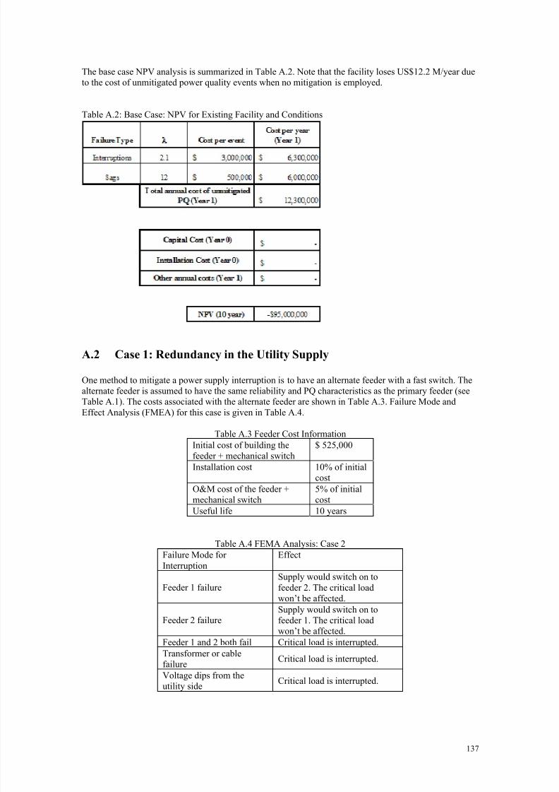
8/20/2019 CIGRE 467 - Economic Framework for Power Quality
http://slidepdf.com/reader/full/cigre-467-economic-framework-for-power-quality 138/151
137
The base case NPV analysis is summarized in Table A.2. Note that the facility loses US$12.2 M/year dueto the cost of unmitigated power quality events when no mitigation is employed.
Table A.2: Base Case: NPV for Existing Facility and Conditions
A.2 Case 1: Redundancy in the Utility Supply
One method to mitigate a power supply interruption is to have an alternate feeder with a fast switch. Thealternate feeder is assumed to have the same reliability and PQ characteristics as the primary feeder (seeTable A.1). The costs associated with the alternate feeder are shown in Table A.3. Failure Mode and
Effect Analysis (FMEA) for this case is given in Table A.4.
Table A.3 Feeder Cost InformationInitial cost of building thefeeder + mechanical switch
$ 525,000
Installation cost 10% of initialcost
O&M cost of the feeder +mechanical switch
5% of initialcost
Useful life 10 years
Table A.4 FEMA Analysis: Case 2
Failure Mode forInterruption
Effect
Feeder 1 failureSupply would switch on tofeeder 2. The critical loadwon’t be affected.
Feeder 2 failureSupply would switch on tofeeder 1. The critical loadwon’t be affected.
Feeder 1 and 2 both fail Critical load is interrupted.Transformer or cablefailure
Critical load is interrupted.
Voltage dips from theutility side
Critical load is interrupted.

8/20/2019 CIGRE 467 - Economic Framework for Power Quality
http://slidepdf.com/reader/full/cigre-467-economic-framework-for-power-quality 139/151
138
The two-feeder system introduces redundancy in the power supply. A reliability block diagram (RBD) forinterruption failure is shown in Figure A.2. For the reliability calculations, a common-mode factor of 0.05is assumed. The QRA analysis results are shown in Table A.5. For the cost analysis, an equipment life often years is assumed.
Feeder 1
Feeder 2
Local
switchgear
Figure A.2. Adding a Redundant Utility Feeder
Table A.5 Ten-year NPV results for a Redundant Feeder
Adding a redundant feeder to this facility does nothing to mitigate voltage dips, but significantly reducesthe impact of protracted interruptions, thereby improving the NPV of unmitigated PQ by approximately$40M.
A.3 Case 2: Applying a Battery UPS
Case 1 examined the benefit of reducing the impact of long outages. However, the cost impact of voltagedips is considerably greater, making it likely that the most beneficial mitigation option will likely includea dip-mitigation solution. This case considers a battery UPS for dip ride-through. Details of the UPS
configuration and cost are given in Table A.6.
Table A.6 UPS InformationFailure rate of each unit 1 failure/yrRepair time per unit 6 hours/yrRedundancy 2 out of 3Common-mode factor for 2-out-of-3 and 3-out-of-3failure mode
0.01
Initial cost of three units $1,000,000Installation cost $100,000O&M cost/yr $100,000UPS life span 10 years

8/20/2019 CIGRE 467 - Economic Framework for Power Quality
http://slidepdf.com/reader/full/cigre-467-economic-framework-for-power-quality 140/151
139
FEMA analysis for this case is shown in Table A.7. N-1 redundancy is assumed. Therefore, the UPSsystem would protect the load even if one unit (out of three) fails. A common-mode failure factor of 0.01is assumed for the redundancy calculations. The RBD for the UPS configuration is shown in Figure A.3.
Table A.7 FEMA Analysis: Case 3Failure Mode for Voltage
Dips
Effect
1 out of 3 UPS units fails. Critical load will still be protected.
2 out of 3 units fail. Critical load would beexposed to dips.
3 out of 3 units fail. Critical load would beexposed to dips.
UPS 2
UPS 3
Critical Load
UPS 1
By-pass switch
2 out of 3 UPS system
Fig. A.3 NPV Calculation for Adding Redundant UPS
As shown in Table A.8, adding redundant UPSs to protect critical loads reduces the average number of
unmitigated voltage dips from 12 to 0.0135 per year, resulting in substantial savings and a positive net present value.
Table A.8 10-year NPV Results: Redundant UPS
Because of its impact on voltage dips, a redundant UPS has a profound impact on reduction ofunmitigated PQ—all but eliminating these costs while adding capital and ongoing maintenance costs. Theoverall improvement in NPV with this option is over $90M (i.e., -$2M – (-$95M) = $93M).
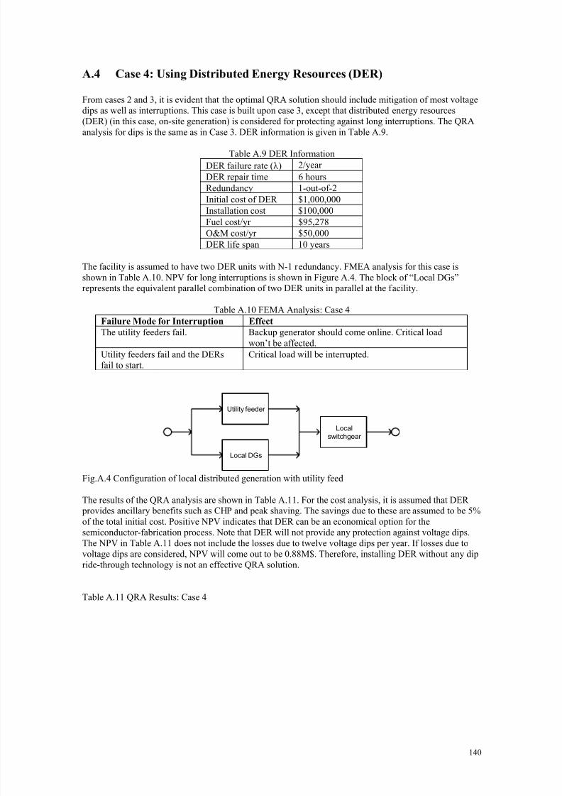
8/20/2019 CIGRE 467 - Economic Framework for Power Quality
http://slidepdf.com/reader/full/cigre-467-economic-framework-for-power-quality 141/151
140
A.4 Case 4: Using Distributed Energy Resources (DER)
From cases 2 and 3, it is evident that the optimal QRA solution should include mitigation of most voltagedips as well as interruptions. This case is built upon case 3, except that distributed energy resources(DER) (in this case, on-site generation) is considered for protecting against long interruptions. The QRAanalysis for dips is the same as in Case 3. DER information is given in Table A.9.
Table A.9 DER InformationDER failure rate (λ) 2/yearDER repair time 6 hoursRedundancy 1-out-of-2Initial cost of DER $1,000,000Installation cost $100,000Fuel cost/yr $95,278O&M cost/yr $50,000DER life span 10 years
The facility is assumed to have two DER units with N-1 redundancy. FMEA analysis for this case is
shown in Table A.10. NPV for long interruptions is shown in Figure A.4. The block of “Local DGs”represents the equivalent parallel combination of two DER units in parallel at the facility.
Table A.10 FEMA Analysis: Case 4Failure Mode for Interruption Effect
The utility feeders fail. Backup generator should come online. Critical loadwon’t be affected.
Utility feeders fail and the DERsfail to start.
Critical load will be interrupted.
Utility feeder
Local DGs
Localswitchgear
Fig.A.4 Configuration of local distributed generation with utility feed
The results of the QRA analysis are shown in Table A.11. For the cost analysis, it is assumed that DER provides ancillary benefits such as CHP and peak shaving. The savings due to these are assumed to be 5%of the total initial cost. Positive NPV indicates that DER can be an economical option for thesemiconductor-fabrication process. Note that DER will not provide any protection against voltage dips.The NPV in Table A.11 does not include the losses due to twelve voltage dips per year. If losses due to
voltage dips are considered, NPV will come out to be 0.88M$. Therefore, installing DER without any dipride-through technology is not an effective QRA solution.
Table A.11 QRA Results: Case 4

8/20/2019 CIGRE 467 - Economic Framework for Power Quality
http://slidepdf.com/reader/full/cigre-467-economic-framework-for-power-quality 142/151
141
Distributed generation is able to mitigate the duration of power outages; however, it’s lack of impact onvoltage dips is a strong disadvantage in this particular analysis. At $44M, the overall improvement in
NPV of this option is roughly comparable to that of a redundant power feed (-$51M – (-$95M) = $44M).
B Case Comparison and Sensitivity
The results of the Base Case and three alternative cases are illustrated in Figure B.1. Although a myriadof other options can be considered, among the three cases, Case 2: Battery UPS offers the best 10-year
NPV and should be seriously considered, along with other solutions that mitigate the impact of voltagedips.
It is also important to note, however, that the other options may offer benefits not taken into account inthis analysis, such as improved safety, environmental issues, or options for combined heat and power
(CHP) or cogeneration. These and many other issues can be considered in the NPV analysis depending onthe sophistication of the application and those designing it. The key is that all cases considered be treatedequivalently.
Comparison of NPV Cases
-$100,000,000
-$80,000,000
-$60,000,000
-$40,000,000
-$20,000,000
$0
Base Case Case 1: Redundant
Feeder
Case 2: Battery
UPS
Case 3: On-Site
Generation
Cases
N P V
( 1 0 - y r )
Figure B.1 NPV Values for Mitigation Cases
It is also important to consider the sensitivity of such an analysis to variations in the input parameters
used—in particular, the number of voltage dips assumed per year can have a profound impact on theresults of the NPV calculations. For example, if the true cost of voltage dips to this facility were actually

8/20/2019 CIGRE 467 - Economic Framework for Power Quality
http://slidepdf.com/reader/full/cigre-467-economic-framework-for-power-quality 143/151
142
$250,000 per event rather than $500,000, the economic analysis would be impacted as illustrated inFigure B.2 below. Although the relative rankings of the various solutions considered here are notchanged, the disparity in their impact on 10-year NPV is considerably reduced. For PQ solutions thataddress only voltage dips (such as dynamic voltage restorers, etc.), reassessment of the cost of individualdips would likely have a profound impact on economic performance.
Comparison of NPV Cases
-$80,000,000
-$60,000,000
-$40,000,000
-$20,000,000
$0
Base Case Case 1: Redundant
Feeder
Case 2: Battery
UPS
Case 3: On-Site
Generation
Cases
N P V
( 1 0 - y r )
Figure B.2 NPV Values for Mitigation Cases with reduced impact of voltage dips
8/20/2019 CIGRE 467 - Economic Framework for Power Quality
http://slidepdf.com/reader/full/cigre-467-economic-framework-for-power-quality 144/151
143
REFERENCES
[1] Bollen, M., Verde, P., 2008. A framework for regulation of rms voltage and short-duration under
and overvoltages. IEEE Transactions on Power Delivery. Vol. 23, Issue 4, Oct. 2008, pages: 2105 –2112.[2] NRS, 2004. Electricity Supply - Quality of supply - Part 2: Voltage characteristics, compatibilitylevels, limits, and assessment methods. NRS 048-2:2003. NRS, Pretoria, South Africa.[3] ERGEG, 2007. Towards voltage quality regulation in Europe. Conclusion paper E07-EQS-15-03. Available from: [www.ergeg.org].[4] CEER, 2005. Third Benchmarking Report on Quality of Electricity Supply. Available fromwww.energy-regulators.eu.[5] CEER, 2008. Fourth Benchmarking Report on Quality of Electricity Supply. Available fromwww.energy-regulators.eu.[6] ERD, 2000. Contrat d'accès au réseau public de distribution d'électricité pour un siteconsommateur éligible raccordé en moyenne tension. Available (in French) from:[www.edfdistribution.fr].
[7] Seljeseth, H., Sand, K., Samdal, K., 2005. Quality of supply regulation in Norway: going beyondEN 50160. In: CIRED 2005, International conference on electricity distribution, Turin, Italy].[8] P. Heine, P. Pohjanheimo, M. Lehtonen, and E. Lakervi, “A method for estimating the frequencyand cost of voltage dips,” IEEE Transactions on Power Systems, vol. 17, pp. 290 – 296, 2002.[9] P. Heine, P. Pohjanheimo, M. Lehtonen, and E. Lakervi, “Estimating the annual frequency andcost of voltage dips for customers of five Finnish distribution companies,” presented at ElectricityDistribution, 2001. Part 1: Contributions. CIRED. 16th International Conference and Exhibition on (IEEConf. Publ No. 482), 2001.[10] S. Quaia and F. Tosato, “Interruption costs caused by supply voltage dips and outages in smallindustrial plants: A case study and survey results,” in The IEEE Region 8 EUROCON. Computer as aTool , vol. 2, 2003, pp. 258 – 262, vol.2.[11] M. M. A. Aziz, G. A. A. Salam, and S. M. Kozman, “Cost and mitigation of voltage dip forindustrial plants,” presented at Electrical, Electronic and Computer Engineering, 2004. ICEEC ’04. 2004
International Conference on.[12] H. Arango, E. G. Domingues, J. P. G. Abreu, and D. M. Camposilvan, “Applying real optionsmethodology to value electrical PQ projects,” presented at Harmonics and Quality of Power, 2002. 10thInternational Conference on, 2002.[13] S. Quaia and F. Tosato, “A method for the computation of the interruption costs caused bysupply voltage dips and outages in small industrial plants,” presented at EUROCON 2003. Computer as aTool. The IEEE Region 8, 2003.[14] R. Lamedica, A. Patrizio, A. Prudenzi, E. Tironi, and D. Zaninelli, “PQ costs and upgradingsolutions: The energy centre,” presented at Harmonics and Quality of Power, 2000. Proceedings. NinthInternational Conference on, 2000.[15] J. V. Milanovic and C. P. Gupta, “Probabilistic assessment of financial losses due tointerruptions and voltage dips – Part I: The methodology,” IEEE Transactions on Power Delivery, vol.21, pp. 918 – 924, 2006.
[16] J. V. Milanovic and C. P. Gupta, “Probabilistic assessment of financial losses due tointerruptions and voltage dips – Part II: Practical implementation,” IEEE Transactions on Power
Delivery, vol. 21, pp. 925 – 932, 2006.[17] M. McGranaghan and B. Roettger, “Economic evaluation of PQ,” IEEE Power Engineering Review, vol. 22, pp. 8 – 12, 2002.[18] G. J. Lee, M. M. Albu, and G. T. Heydt, “A PQ index based on equipment sensitivity, cost, andnetwork vulnerability,” IEEE Transactions on Power Delivery, vol. 19, pp. 1504 – 1510, 2004.[19] IEEE recommended practice for evaluating electric power system compatibility with electronic
process equipment. IEEE Standard 1346-1998, 1998.[20] J. Y. Chan, J. V. Milanovic, and A. Delahunty, “Generic failure risk assessment of industrial
processes due to voltage dips,” IEEE Transactions on Power Delivery, to be published.[21] P. Pohjanheimo and M. Lehtonen, “Introducing Prob-A-Dip - A probabilistic method for voltagedip management,” in 11th International Conference on Harmonics and Quality of Power , 2004, pp. 250-
254.
8/20/2019 CIGRE 467 - Economic Framework for Power Quality
http://slidepdf.com/reader/full/cigre-467-economic-framework-for-power-quality 145/151
144
[22] J. Y. Chan and J. V. Milanovic, “Methodology for assessment of financial losses due to voltagedips and short interruptions,” in 9th International Conference on Electrical PQ and Utilisation.Barcelona, 2007.[23] J. Y. Chan and J. V. Milanovic, “Severity indices for assessment of equipment sensitivity tovoltage dips and short interruptions,” in IEEE PES General Meeting 2007 . Tampa, Florida, 2007.[24] J. Wang, S. Chen, and T. T. Lie, “Estimating economic impact of voltage dips,” vol. 1, 2004
International Conference on Power System Technology, POWERCON 2004. Singapore: Institute ofElectrical and Electronics Engineers Inc., New York, NY 10016 – 5997, United States, 2004, pp. 350 –355.[25] S. Y. Yun and J. C. Kim, “An evaluation method of voltage dip using a risk assessment model in
power distribution systems,” International Journal of Electrical Power and Energy Systems , vol. 25, pp.829 – 839, 2003.[26] R. C. Leborgne, J. M. C. Filho, J. P. G. d. Abreu, T. C. Oliveira, A. A. Postal, and L. H.Zaparoli, “Alternative methodology for characterization of industrial process sensitivity to voltage dips,”in IEEE Bologna PowerTech Conference Proceedings, vol. 3. Bologna, Italy, 2003, pp. 6.[27] F.Tosato and S.Quaia, “A method for the computation of the interruption costs caused by supplyvoltage dips and outages in small industrial plants,” in The IEEE Region 8 EUROCON 2003. Computer
as a Tool , vol. 2, 2003, pp. 249 – 253.[28] C. P. Gupta, J. V. Milanovic, and M. T. Aung, “The influence of process equipment composition
on financial losses due to voltage dips,” in 11th International Conference on Harmonics and Quality of Power , Lake Placid, NY, United States, 2004, pp. 28 – 34.[29] M. Delfanti, E. Fumagalli, P. Garrone, L. Grilli, and L. L. Schiavo, “Towards voltage qualityregulation in Italy”. Submitted to IEEE Transactions on Power Delivery.[30] J. T. Crozier and W. N. Wisdom, “A PQ and reliability index based on customer interruptioncosts,” IEEE Power Engineering Review, vol. 19, pp. 59 – 61, 1999.[31] R. Ghandehari and A. Jalilian, “Economical impacts of PQ in power systems,” Bristol, UnitedKingdom, 2004.[32] Y. Shih-An, S. Chun-Lien, and C. Rung-Fang, “Assessment of PQ cost for high-tech industry,”
presented at Power India Conference, 2006 IEEE, 2006.[33] M. F. McGranaghan and W. C. Roettger, “The economics of custom power,” presented atTransmission and Distribution Conference and Exposition, 2003 IEEE PES, 2003.[34] M. Lehtonen and B. Lemstrom, “Comparison of the methods for assessing the customers outage
costs,” in International Conference on Energy Management and Power Delivery, vol. 1, 1995, pp. 1 – 6.[35] IEEE recommended practice for monitoring electric PQ. IEEE Standard 1159-1995, 1995.[36] B. Lee, G. K. Stefopoulos, and A. P. S. Meliopoulos, “Unified reliability and PQ index,” in 12th International Conference on Harmonics and PQ, Portugal, 2006.[37] J. V. Milanovic and N. Jenkins, “PQ cost for manufacturing industries,” Paris, 2003.[38] F. Carlsson and P. Martinsson, “Does it matter when a power outage occurs? – A choiceexperiment study on the willingness to pay to avoid power outages,” Department of Economics,Gothengurg University, 2004.[39] F. Carlsson and P. Martinsson, “Willingness to pay among Swedish households to avoid poweroutages – A random parameter Tobit model approach,” Department of Economics, GothenburgUniversity, 2004.[40] R. Targosz and J. Manson, “Pan European LPQI PQ survey,” in CIRED 19th InternationalConference on Electricity Distribution, Vienna, 2007.
[41] K. Samdal, G. Kjølle, B. Singh, and F. Trengereid,. Customers’ interruption costs: What’s the problem? In: CIRED 2003, International Conference on Electricity Distribution, Barcelona, Spain.[42] K. K. Kariuki and R. N. Allan, “Evaluation of reliability worth and value of lost load,” IEE Proceedings: Generation, Transmission and Distribution, vol. 143, pp. 171 – 180, 1996.[43] T. Andersson and D. Nilsson, “Test and evaluation of voltage dip immunity,” STRI AB andVatenfall AB, 27 Nov. 2002.[44] D. Chapman, “The cost of poor PQ,” Copper Development Association, November 2001.[45] M. J. Sullivan, T. Vardell, and M. Johnson, “Power interruption costs to industrial andcommercial consumers of electricity,” IEEE Transactions on Industry Applications, vol. 33, pp. 1448 –1457, 1997.[46] K. H. LaCommare and J. H. Eto, “Understanding the cost of power interruption to U.S.electricity consumers,” Ernest Orlondo Lawrence Berkeley National Laboratory, LBNL-55718, 2004.[47] Primen, “The cost of power disturbances to industrial & digital economy companies,” EPRI
CEIDS, June 2001.

8/20/2019 CIGRE 467 - Economic Framework for Power Quality
http://slidepdf.com/reader/full/cigre-467-economic-framework-for-power-quality 146/151
145
[48] EPRI, “Incentives and penalties for electrical PQ under performance based regulations,” CEATechnologies Inc. (CEATI) T044700-5124, November 2005.[49] B. H. Chowdhury, “PQ,” in IEEE Potentials: The Magazine for Up-and-Coming Engineers,2001, pp. 5 – 11.[50] J. D. Lamoree, “Cost of Outages,” Enernex Corporation, October 2004.[51] Y. Shih-An, L. Chan-Nan, E. Liu, H. Yu-Chang, and H. Chinug-Yi, “Assessment of interruption
cost to high tech industry in Taiwan,” presented at Transmission and Distribution Conference andExposition, 2001 IEEE/PES, 2001.[52] S. B. Choi, K. Y. Nam, D. K. Kim, S. H. Jeong, H. S. Ryoo, J. D. Lee, “Evaluation ofinterruption costs for industrial customers in Korea,” presented at Power System Conference andExposition, 2006. PSCE’06.[53] G. Linhofer, P. Maibach, and F. Wong, “PQ devices for short term and continuous voltagecompensation,” in International PQ Conference 2002, Singapore, 2002.[54] E. Emanuel, M. Yang, and D. J. Pileggi, “The engineering economics of power systemharmonics in subdistribution feeders: A preliminary study”, IEEE Transactions on Power Systems, Vol. 6,
No. 3, August 1991, pp. 1092 – 1098.[55] A. E. Emanuel, J. Pileggi, T. J. Gentile, E. M. Gulachenski, D. Sorensen, and J. Janczak,“Distribution feeders with nonlinear loads in the Northeast U.S.A.: Part I – Voltage distortion forecast”,IEEE/PES Winter Meeting, Jan. 1994, New York (USA), 94 WM 089-3 PWRD.
[56] J. Pileggi, T. J. Gentile, A. E. Emanuel, E. M. Gulachenski, M. Breen, D. Sorensen, and J.Janczak, “Distribution feeders with nonlinear loads in the Northeast U.S.A.: Part II – Economicevaluation of harmonic effects”, IEEE/PES Winter Meeting, Jan. 1994, New York (USA), 94 WM 090-1 PWRD.[57] P. Caramia, G. Carpinelli, E. Di Vito, A. Losi, and P. Verde, “Probabilistic evaluation of theeconomical damage due to harmonic losses in industrial energy systems”, IEEE Transactions on Power Delivery, vol. 11, no. 2, April 1996, pp. 1021 – 1031.[58] P. Caramia, G. Carpinelli, A. Losi, A. Russo, and P. Verde, “A simplified method for the
probabilistic evaluation of the economical damage due to harmonic losses”, 8th Int. Conference onHarmonics and Quality of Power, October 1998, Athens (GR), pp. 767 – 776.[59] G. Mazzanti, A. Cavallini, G.C. Montanari, P. Caramia, G. Carpinelli, and P. Verde, “Anapproach to life estimation of electrical plant components in the presence of harmonic distortion,”
presented at ICHQP 2004, Lake Placid (NY), USA.
[60] P. Verde, “Cost of harmonic effects as meaning of standard limits,” Proceedings. Ninth International Conference on Harmonics and Quality of Power, 2000, Volume 1, 1 – 4 Oct. 2000 pp. 257 – 259, vol.1.[61] P. Caramia and P. Verde, “Cost-related harmonic limits,” Power Engineering Society WinterMeeting, 2000. IEEE Volume 4, 23 – 27 Jan. 2000, pp. 2846 – 2851.[62] A. Cavallini, D. Fabiani, G. Mazzanti, G.C. Montanari, and A. Contin, “Voltage endurance ofelectrical components supplied by distorted voltage waveforms,” Proc. 2000 International Symposium onElectrical Insulation, pp. 73 – 76, Anaheim, California (USA), April 2000.[63] D.Gallo, R. Langella, and A. Testa, “Predicting voltage stress effects on MV/LV components,”2003 IEEE Bologna PowerTech Conference, June 23 – 26, Bologna, Italy. Volume 2.[64] IEEE Task Force, “The effects of power system harmonics on power system equipment andloads,” IEEE Transactions Power Apparatus and Systems, Vol. PAS-104, Sept 1985, pp. 2555 – 2563.[65] IEEE Task Force, “Effects of harmonics on equipment,” IEEE Transactions on Power Delivery,
Vol. 8, April 1993, pp. 672 – 680.[66] M. A. Miner, “Cumulative damage in fatigue,” Journal of Applied Mechanics, September 1945,
pp. A159 – A163.[67] G. J. Anders, Rating of electric power cables, Mc Graw hill, IEEEE Press, Piscataway, NJ, 1997.[68] L. Simoni, “Fundamentals of endurance of electrical insulating materials,” CLUEB Publ., 1st issue 1985, 2nd issue 1993.[69] Z. Kowalski, Unbalance in Power Systems [in Polish], PWN 1987.[70] Y. Baghzouz et al., “Time-varying harmonics. II. Harmonic summation and propagation,” IEEETransactions on Power Delivery, Volume 17, Issue 1, Jan. 2002, pp. 279 – 285.[71] R. Billinton and R. N. Allan, Reliability Evaluation of Power Systems, Plenum Press, New York,1994.[72] Math H. J. Bollen, Under PQ problems: Voltage dips and interruptions, IEEE PowerEngineering Series, 2000.
[73] L. E. Conrad and M. H. J. Bollen, “Voltage dip coordination for reliable plant operation,” IEEETransactions on Industry Applications, Vol. 33, No. 6, Nov./Dec. 1997, pp. 1459 – 1463.

8/20/2019 CIGRE 467 - Economic Framework for Power Quality
http://slidepdf.com/reader/full/cigre-467-economic-framework-for-power-quality 147/151
146
[74] M. F. McGranaghan, D. R. Mueller, and M. J. Samotyj, “Voltage dips in industrial systems,” IEEE Transactions on Industry Applications, Vol. 29, No. 2, March/April 1993, pp. 397 – 402.[75] S. Z. Djokic, K. Stockman, J.V. Milanovic, J. J. M. Desmet, and R. Belmans, “Sensitivity of ACadjustable speed drives to voltage dips, short interruptions and under-voltage transients,” IEEETransactions on Power Delivery (in press). (Manuscript no. TPWRD- 00380-2003 accepted for
publication in November 2003).
[76] EPRI Brief Report No. 46, “Performance of a hold-in device for relays, contactors and motor-starters,” October 1998. (http://www.portlandgeneral.com/business/products/business power problems/PQschool/brief46.pdf ).[77] E. Collins and M. Bridgwood, “The impact of power system disturbances on AC-coilcontactors,” Proc. IEEE Textile, Fiber and Film Industry Technical Annual Conference, Greenville, USA,6-8 May 1997.[78] S. Z. Djokic, J. V. Milanovic, and D. S. Kirschen, “Sensitivity of AC coil contactors to voltagedips, short interruptions and under-voltage transients,” IEEE Transactions on Power Delivery, Vol 19,
No. 3, 2004, pp. 1299 – 1307.[79] R. Caldon, M. Fauri, and L. Fellin, “Voltage dip effects on continuous industrial processes:Desensitizing study for textile manufacture,” Proc. of Second Int. Conf. on PQ: End-Use Applicationsand Perspectives, Atlanta, USA, Sept. 28 – 20, 1992, pp. D – 13: 1-6.[80] S. Z. Djokic, J. Desmet, G. Vanalme, J.V. Milanovic, and K. Stockman, “Sensitivity of personal
computers to voltage dips, short interruptions,” IEEE Transactions on Power Delivery (in press). (Manuscript no. TPWRD- 00159-2003 accepted for publication in November 2003 ).[81] J. Lamoree, D. Mueller, P. Vinett, W. Jones, and M. Samotyj, “Voltage dip analysis casestudies,” IEEE Transactions on Industry Applications, Vol. 30, No. 4, July/August 1994, pp. 1083 –1089.[82] R. G. Brown and P. Y. C. Hwang, Introduction to random signals and applied Kalman filtering ,John Wiley and Sons, New York, 1997.[83] R. Billinton and R. N. Allan, Reliability evaluation of engineering systems, Plenum Press, NewYork, 1992.[84] M. T. Aung, J. V. Milanović, and P. A. Simmons, “Automated comprehensive assessment andvisualization of voltage dip performance,” CD Rom of the 11
th IEEE International Conference on Harmonics and Quality of Power, ICHQP 2004, Lake Placid, NY, USA, September 12 – 15, 2004.[85] G. Olguin and M. H. J. Bollen, “The method of fault positions for stochastic prediction of
voltage dips: A case study,” CD-ROM of the International Conference on Probabilistic Methods Appliedto Power Systems, Naples, Italy, September 22 – 26, 2002.[86] G. Mazzanti, G. Passarelli, A. Russo, and P. Verde, “The effects of voltage waveform factors oncable life estimation using measured distorted voltages,” Power Engineering Society General Meeting,2006. IEEE, 18 – 22 June 2006, p. 8.[87] P. H. Allen, and A. Tustin, “The aging process in electrical insulation: A tutorial summary,”IEEE Transactions on Electr. Insul., vol. EI-7, 1972, pp. 153 – 161.[88] A. Cavallini, G. Mazzanti, G. C. Montanari, and D. Fabiani, “The effect of power systemharmonics on cable endurance. A critical review to IEEE std. 519 voltage distortion limits,” Proc. IASAnnual Meeting, Roma (Italy), October 2000.[89] G. C. Montanari and G. Pattini, “Thermal endurance of insulating materials,” IEEE Transactions
on Electrical Insulation, Vol. 21, No. 1, February 1986, pp. 66 – 75.[90] J. Manson, Business model for investing in PQ solutions, PQ application guide background
notes, Chapter 2 – “Costs,” www.lpqi.org.[91] A. H. Eltom and N. S. Moharari, “Motor temperature estimation incorporating dynamic rotorimpedance,” IEEE Transactions on Energy Conversion, vol. 6, 1991, pp. 107 – 113.[92] J. Aubin, R. Bergeron, and R. Morin, “Distribution transformer overloading capability undercold-load pickup conditions,” IEEE Transactions on Power Delivery, vol. 4, 1990, pp. 1883 – 1890.[93] IEC Standard, Calculation of the continuous current rating of cables. Part I: 100% load factor, Pub. n. 287, 1982.[94] R. Gretsch and G. Krost, “Moglichkeiten zur bestimmung der frequenzabhangigennetzimpedanzen,” EtzArchiv, 1979, H2, pp. 45 – 52.[95] R. Gretsch and G. Krost, “Messung der oberschwingungs-impedanzen von verbrauchern,”EtzArchiv, 1981, H1, pp. 13 – 22.[96] V. Isastia, M. Perez de Vera, and M. Scarano, “Distribuzione delle perdite nel rame nelle gabbiedei motori asincroni a barra alta alimentati con tensioni deformate,” Italian Research Council, n. 49,
Naples (Italy), 1983.

8/20/2019 CIGRE 467 - Economic Framework for Power Quality
http://slidepdf.com/reader/full/cigre-467-economic-framework-for-power-quality 148/151
147
[97] Verde Paola, Carpinelli Guido, and F. Gagliardi, “Probabilistic modelings for harmonic penetration studies in power systems,” 5th IEEE International Conference on Harmonics in PowerSystems, Atlanta (USA), September 1992, pp. 35 – 40.[98] P. Caramia, G. Carpinelli, F. Rossi, and P. Verde, “Probabilistic iterative harmonic analysis of
power systems,” Generation, Transmission and Distribution, IEE Proceedings, Volume 141, Issue 4, July1994, pp. 329 – 338.
[99] M. Munasinghe and M. Gellerson, "Economic criteria for optimizing power system reliabilitylevels", The Bell Journal of Economics, vol. 10, pp. 353-365, 1979.[100] K. K. Kariuki and R. N. Allan, “Application of customer outage costs in system planning, designand operation,” IEE Proceedings on Generation, Transmission and Distribution, Vol. 143, No. 4, July1996, pp. 305 – 312.[101] EN 50160:2007 Ed.3 "Voltage characteristics of electricity supplied by public distributionnetworks".[102] S..L Lau and M.R. Tamjis “The economics of power quality,” IET Power Engineer, pp. 38-41December/January 2006/07.[103] Ming Su, Gengyin Li, Ming Zhou , and Jin Yang, “A power quality service pricing approachconsidering treatment expenses and stop loss insurance,” Power Tech 2007, Paper no 626.[104] D. M. Didden, “Voltage disturbances – considerations for choosing the appropriate dip mitigationdevice,” in Power Quality Application Guide, Copper Development Association, 2005.
[105] European Information Technology Observatory (EITO), Press release 2004.[106] EURELECTRIC NE Standardisation / N-EMC & Harmonics. For PQ costs study.Considerations on voltage dips and short supply interruptions. Gerhard Bartak.[107] „Auftretenswahrscheinlichkeit von Spannungseinbrüchen verschiedener Restspannung undDauer für Kundenanlagen in Mittelspannungsnetzen“, Diplomarbeit am Institut für Elektrische Anlagender TU Graz, 2000.[108] A. Haber: „Analyse von Spannungseinbrüchen und mögliche Abhilfemassnahmen in einemIndustriebetrieb“, Diploma thesis, TU Graz/Prof. Fickert, June 2001.[109] M. Schmidt: „Minimierung der Kundenausfallskosten unter Berücksichtigung der automatischenWiedereinschaltung“, Diploma thesis, TU Graz/Prof. Fickert, April 2003.[111] Knut Samdal et al.: “Customers’ interruption costs – what’s the problem ?”, 17th CIREDConference, Barcelona, 12 – 15 May 2003, Session 6, Paper No 31.[112] Norwegian water resources and energy directorate (NVE). Energy and regulation department.
[113] Renner, H.; Fickert, L.: “Costs and Responsibility of Power Quality in the Deregulated ElectricityMarket”, TU Graz, Institut für Elektrische Anlagen und Hochspannungstechnik, Abteilung ElektrischeAnlagen, 2000.[114] Copper Development Association: Power Quality Application Guide, March 2001.[115] G. Brauner, CH. Hennerbichler: “Empfindlichkeit von elektrischen Geräten gegenüberSpannungseinbrüchen und Kurzzeitunterbrechungen“, Study on behalf of VEÖ-EFG, 2001.[116] IEC 61000-4-7: Electromagnetic compatibility (EMC) - Part 4-7: Testing and measurementtechniques - General guide on harmonics and interharmonics measurements and instrumentation, for
power supply systems and equipment connected thereto.[117] IEC 61000-4-30: Electromagnetic compatibility (EMC) - Part 4-30: Testing and measurementtechniques - Power quality measurement methods.[118] F., Porrino, A., Chiumeo, R., Malgarotti, S., 2007. The power quality monitoring of the MVnetwork promoted by the Italian regulator. Objectives, organisation issues, 2006 statistics. In: CIRED
2007, International conference on electricity distribution, Vienna, Austria.[119] S. C. Vegunta and J. V. Milanović, Estimation of costs of Downtime of Industrial Process Dueto Voltage Sags.[120] PQ measurement campaign in Austria, 2000 – 2004, VEÖ-Journal: Part I, H.11/2000; Part II,H.7/2001; Part III, H.8/2001; Part IV, H.8/2002; Part V, H.2-3/2003; Part VI, H.10/2003, Part VII, H.1-2/2004, Part VIII, H. 10/2004.[121] EURELECTRIC Report “Power Quality in European Electricity Supply Networks” – 2ndedition, November 2003.[122] Qualita’ del servizio di trasmissione - Rapporto annuale per l’anno 2006, 30 april 2007, www.Terna.it.[123] Power quality: Customer financial impact/risk assessment tool, BC Hydro, A04-587b, 2005.[124] IEEE recommended practice for evaluating electric power system compatibility with electronic
process equipment, IEEE Std 1346-1998, 1998.
[125] M. M. Izhwan, M. Norman, and M. A. M. Radzi, The effects of power quality to the industries,,5th Student Conference on Research and Development, SCOReD, 2007.
8/20/2019 CIGRE 467 - Economic Framework for Power Quality
http://slidepdf.com/reader/full/cigre-467-economic-framework-for-power-quality 149/151
148
[126] M. F. Han and K. Yeon-hee, Samsung Elec says outage loss not to top $54 mln, in Reuters,2007.[127] Samsung shares lower on concerns over power outage-production loss, in AsiaPulse News, 2007.[128] R. B. Chandler, M. J. Jellison, J. W. Skogsberg, and T. Moore, NACE 02056 advanced drillstring metallurgy provides enabling technology for critical sour drilling, 2002.[129]Y. Levendel, “The manufacturization of the software quality improvement process, IEEE Region 10
International Conference on EC3-Energy, Computer, Communication and Control Systems (TENCON),1991.[130] IEC/TR 61000-3-6 (2008). Electromagnetic compatibility (EMC) - Part 3-6: Limits - Assessmentof emission limits for the connection of distorting installations to MV, HV and EHV power systems[131] Applying QRA Methodology in Power System Applications, EPRI, Palo Alto, CA, 2004.[132] Analysis of Extremely Reliable Power Delivery System, EPRI, Palo Alto, CA, 2002.[133] A. G. Maitra and T. Short, “Assessing financial feasibility of PQ improvement devices usingmonte carlo simulations,” presented at Probabilistic Methods Applied to Power Systems, 8th InternationalConference, September 2004.[134] L. Conrad, K. Little, and C. Grigg, “Predicting and preventing problems associated with remotefault-clearing voltage dips,” IEEE Transactions on Industry Applications, Vol. 27, No. 1, Jan./Feb. 1991,
pp.167-172.[135] L. E. Conrad and M. H. J. Bollen, “Voltage dip coordination for reliable plant operation,” IEEE
Transactions on Industry Applications, Vol. 33, No. 6, Nov./Dec. 1997, pp. 1459-1463.[136] J. Lamoree, D. Mueller, P. Vinett, W. Jones, and M. Samotyj, “Voltage dip analysis casestudies,” IEEE Transactions on Industry Applications, Vol. 30, No. 4, July/August 1994, pp. 1083-1089.[137] IEEE recommended practice for emergency and standby power systems for industrial andcommercial applications (IEEE orange book), New York, IEEE Std. 446-1995.[138] Information Technology Industry Council: “ITI (CBEMA) curve and application note,”Washington, 1998, revised 2000, (http://www.itic.org/technical/iticurv.pdf).[139] Semiconductor Equipment and Materials International: “SEMIF47-0200, specification forsemiconductor processing equipment voltage dip immunity,” SanJose, USA, 2000.(http://www.semi.org/pubs/semipubs.nsf).[140] S. Z. Djokic, J. Desmet, G. Vanalme, J.V. Milanović, and K. Stockman, “Sensitivity of personalcomputers to voltage dips, short interruptions,” IEEE Transactions on Power Delivery, Vol 20, No. 1,2005, pp. 375-383.
[141] R. Caldon, M. Fauri, and L. Fellin, “Voltage dip effects on continuous industrial processes:Desensitizing study for textile manufacture,” Proc. of second Int. Conf. on power quality: end-useapplications and perspectives, Atlanta, USA, Sept. 28-20, 1992, pp. D-13: 1-6.[142] S. Z. Djokic, K. Stockman, J.V. Milanović, J. J. M. Desmet, and R. Belmans, “Sensitivity of ACadjustable speed drives to voltage dips, short interruptions and under-voltage transients,” IEEETransactions on Power Delivery , Vol 20, No. 1, 2005, pp. 494-505.[143] EPRI Brief Report No. 46, “Performance of a hold-in device for relays, contactors and motor-starters,” October 1998. (http://www.portlandgeneral.com/business/products/businesspower
problems/power quality school/brief46.pdf).[144] E. Collins and M. Bridgwood, “The impact of power system disturbances on AC-coilcontactors,” Proc. IEEE Textile, Fiber and Film Industry Technical Annual Conference, Greenville, USA,6-8 May 1997.[145] S. Z. Djokic, J.V. Milanović, and D.S. Kirschen, “Sensitivity of AC coil contactors to voltage
dips, short interruptions and under-voltage transients,” IEEE Transactions on Power Delivery, Vol 19, No. 3, 2004, pp. 1299-1307.[146] P. Pohjanheimo, A probabilistic method for comprehensive voltage dip management in powerdistribution systems, PhD Thesis, Helsinki University of Technology, Espoo, Finland, November 2003.[147] S. Z. Djokic, Generalized methodology for the assessment of voltage dip performance indicesand equipment sensitivity, PhD Thesis, UMIST, Manchester, UK, April 2004.(http://www.umist.ac.uk/departments/mcee/research/publications.htm)[148] M. H. J. Bollen, Under power quality problems: voltage dips and interruptions, IEEE PowerEngineering Series, 2000.[149] M. R. A. Qader, Stochastic assessments of voltage dips due to short circuits in electrical networks, PhD thesis, Department of Electrical Power Engineering, Manchester Centre for ElectricalEnergy, UMIST, Manchester, UK. 1997.[150] IEEE Recommended Practice for Evaluating Electric Power System Compatibility with
Electronic Process Equipment, IEEE Std 1346-1998.

8/20/2019 CIGRE 467 - Economic Framework for Power Quality
http://slidepdf.com/reader/full/cigre-467-economic-framework-for-power-quality 150/151
149
[151] M. R. A. Qader, M. H. J. Bollen, and R. N. Allen, “Stochastic prediction of voltage dips in alarge transmission system,” IEEE Transactions on Industry Applications, January/February 1999. Vol. 35,
No. 1: pp. 152-162.[152] G. Olguin and M. H. J. Bollen, “The method of fault positions for stochastic prediction of voltagedips: A case study,” Probabilistic Methods Applied to Power Systems Conference, Naples, Italy,September 22-26, 2002.
[153] M. H. J. Bollen, M. R. Qader, and R. N. Allen, “Stochastic assessment of voltage dips in largetransmission networks theory and case study,” International Conference on Large Electric Networks(CIGRE), August 1998.[154] R. Grover Brown and P. Y. C. Hwang, Introduction to random signals and applied Kalman filtering,John Wiley and Sons, New York, 1997.[155] R. Billinton and R. N. Allan, Reliability evaluation of engineering systems, Plenum Press, NewYork, 1992.[156] J.M.C. Filho, et al., “Analysis of power system performance under voltage dips,” Electrical PowerSystem Research, December, 1999. Vol. 55, No. 3: pp. 211-218.[157] R. Grunbaum, R. Sharma, and J. P. Charpentier, “Improving the efficiency and quality of ACtransmission systems (Draft 3),” Joint World Bank / ABB Power Systems Paper, 24 March, 2000.[158] D. M. Didden, “Voltage disturbances: Considerations for choosing the appropriate dip mitigationdevice,” in Power Quality Application Guide, Copper Development Association, 2005.
[159] A. Baggini and F. Bua, “Investment analysis for PQ solutions,” in Power Quality ApplicationGuide, Copper Development Association: online available: http://www.cda.org.uk/pqp/pqag.htm, May,2007.[160] A. Anderton, ECONOMICS, 4th edition: Harlow: Causeway, 2000.[161] T. L. Minnie, E. G. Gaylon, and T. Phillip, Investment analysis for real estate decisions, DearbornReal Estate Education, 2003.[162] H. D. Keulenaer, “Power quality self-assessment guide,” in Power Quality Application Guide,Copper Development Association: online available: http://www.cda.org.uk/pqp/pqag.htm, May, 2007.[163] A. A. Groppelli and E. Nikbakht, Finance, Barrons Educational Series, Inc., 2000.[164] H. Gregersen and A. Contreras. “Economic assessment of forestry project impacts,” World BankUnited Nations Environment Programme Food and Agriculture Organization of the United Nations, 1995.[165] Oury BA, Roger Bergeron, « Harmonic cost on distribution power system », EPQU, September1999, p5-12
[166] Stavros Papathanassiou, Nikos Drossos, Dimitris Stravaopoulos, « A practical evaluation ofdistribution network losses due to harmonics », CIRED, Vienna 2007[167] ANSI C84.1-2006, American National Standard for Electric Power Systems and Equipment— Voltage Ratings (60 Hertz)

8/20/2019 CIGRE 467 - Economic Framework for Power Quality
http://slidepdf.com/reader/full/cigre-467-economic-framework-for-power-quality 151/151
ACKNOWLEDGMENTS
Members C4.107 - Economic Framework for Voltage Quality
Jose GUTIERREZ IGLESIAS Spain Utility Chairman C4.107 & Coord. Ch. 3Detmar ARLT Germany AcademiaGerhard BARTAK Austria UtilityMath BOLLEN Sweden ResearchDave BYRNE Ireland UtilityDavid CHAPMAN UK Institution Coordinator Chapter 1Alice DELAHUNTY UK Utility Coordinator Chapter 3Philippe EYROLLES France UtilityElena FUMAGALLI Italy AcademiaMats HAGER Sweden IndustryZbigniew HANZELKA Poland AcademiaBill HOWE USA Research Coordinator Chapter 5Rafaël JAHN Belgium Research
Alex McEACHERN USA ManufacturerIan McMICHAEL Australia ResearchJovica V. MILANOVIC UK Academia Coordinator Chapter 2Patxi PAZOS Spain UtilityRoman TARGOSZ Poland Institution Coordinator Chapter 4Mario TREMBLAY Canada ResearchJasper Van CASTEREN Netherlands InstitutionMathieu VAN DEN BERGH USA ManufacturerRaghavan VENKATESH India ManufacturerPaola VERDE Italy Academia Coordinator Chapter 2 and 4
Other former C4.107 members or that collaborate by correspondence:
H i lt d S BRONZEADOB il Utilit