cinquiemes doctoriales de macrofi et seminaire...

CINQUIEMES DOCTORIALES DE MACROFI

ET

SEMINAIRE

DIVERSITE DES SYSTEMES FINANCIERS ET CROISSANCE

22-23 mai 2008

Oil prices and inflation in the euro area: A nonlinear and unstable relationship

Guillaume L'œillet

CREM, Université de Rennes I

Amphi René CASSIN Institut d’Etudes Politiques d’Aix-en-Provence 25, Rue Gaston de Saporta, AIX-EN-PROVENCE

Oil prices and in�ation in the euro area:

A nonlinear and unstable relationship

Guillaume L'oeillet∗ & Julien Licheron

UNIVERSITY OF RENNES 1 - CREM

Preliminary draft - May 2008

Abstract

This paper investigates the relationship between oil prices and headline in�ation in

the euro area. This link has widely evolved since the two big oil shocks of the seventies,

and in�ation nowadays does not reach high levels despite the large oil prices upsurge. We

empirically assess those shifts by estimating a backward Phillips curve on European data

between 1970 and 2007. The results draw two features for the relationship: a diminished

pass-through of oil prices to in�ation and a nonlinear pattern. The declining energy

intensity in the countries belonging to the euro area seems to account for a large part

in the reduction of the in�ationary e�ects of oil prices. The nature of current oil price

increases (mainly driven by world demand), which widely di�er from the oil shocks of the

seventies (caused by disruptions in oil supply), may also provide an explanation for the

smaller impact on in�ation developments.

J.E.L. classi�cation: E31, F41, Q43.

Keywords: In�ation; Phillips curve; Oil prices; Nonlinearity.

∗Corresponding author. Faculté des Sciences Economiques, Université de Rennes 1, 7 place Hoche - CS 86514,35065 Rennes Cedex, France. Tel.: +33.(0)2.23.23.35.60. E-mail address: [email protected]

1

1 Introduction

Since 2001, we have observed a long-lasting and large increase in oil prices, with nominal prices

rising by over 100 percent. Nevertheless, this increase does not translate into much higher

in�ation rates in the euro area. Indeed, headline in�ation in the European Monetary Union

(EMU) remains rather low (with HICP in�ation �uctuating slightly above 2%) in spite of the

revival of a energy price "shock". This situation contrasts with the events following the two

big oil shocks of the seventies, which generated two-digit in�ation rates.

In this paper, we assess the role of oil prices in the dynamics of in�ation and explore the

reasons for the structural shifts in the relationship. We especially search for the existence of a

nonlinearity in the transmission of oil prices into headline in�ation. We also want to test for

the structural stability in the long-term relationship.

Mork (1989), Mory (1993) and Mork, Olsen & Mysen (1994) highlight the existence of

an asymmetric relationship between oil prices and activity by estimating separate coe�cients

for oil prices decreases and increases. According to them, an increase in oil prices reduces

the activity to a larger extent than decreasing oil prices boost the output. Several papers

report the same kind of asymmetry in the oil price-in�ation relationship. Most notably, Hooker

(2002) and LeBlanc & Chinn (2004) use asymmetric oil prices indicators in a Phillips curve

framework and conclude to a signi�cant and immediate e�ect of crude oil prices on headline

in�ation, for the United States and the G-5 countries respectively. Both papers also explore

the structural stability of the relationship. LeBlanc & Chinn (2004) apply recursive estimates

of the coe�cients associated to oil prices, and conclude to a clear decline, especially from 1999.

Hooker (2002) uses a wide set of stability tests, namely the tests from Andrews (1993), Andrews

& Ploberger (1994) and Bai & Perron (1998), and reports a single break in the U.S. oil prices-

in�ation relationship, which seems to be located around 1981 (after the second oil shock). More

recently, Van den Noord & André (2007) and De Gregorio, Landerretche & Neilson (2007) also

work out on this relationship and look for structural shifts in several countries. The �rst paper

bends on the relationship between oil prices and core in�ation for the U.S. and the euro area,

within an augmented Phillips curve framework on two precise sub-samples (1971-1985 and

1986-2006), separated by the large energy prices downturn. As for De Gregorio et al. (2007),

they detect multiple breakpoints for a large sample of countries (34 including less-developed

2

countries) and calculate for each of them a long term pass-through statistic from oil prices to

in�ation. In addition to the methodology, Van den Noord & André (2007) and De Gregorio,

Landerretche & Neilson (2007) share the same conclusions regarding the potential explanations

for the declining relationship between oil prices and in�ation. They point out the reduction

of the energy intensity and consequently the more energy-e�cient use of capital. De Gregorio

et al. (2007) thus distinguish between developed economies and emerging countries regarding

the di�erent degree of the pass-trough from oil prices to in�ation.

In our paper, we also use a traditional Phillips curve extended with oil prices to assess this

relationship in the euro area, while most of the papers cited above focus on the U.S., except

Van den Noord & André (2007) and De Gregorio et al. (2007). In a �rst time, the estimation

of the Phillips curve on a rather large sample (1970-2007) allows for an evaluation of potential

nonlinearity. We thus introduce oil prices under asymmetric speci�cations, as suggested by

Mork (1989) and Hamilton (1996). Then, we search for structural breaks in the relationship

with a Bai-Perron stability test. We estimate the Phillips curve on the sub-samples induced

by the test, and perform rolling estimates for aggregate oil prices. We also face our results

to robustness checks with alternative indicators for in�ation and activity. At last, we provide

several potential explanations to our results.

The results demonstrate a nonlinear pattern in the relationship between crude oil prices

and headline in�ation. The stability tests show that the relationship has also largely evolved

during the last thirty years, and oil prices enter scarcely signi�cant in the second sub-sample.

Concerning potential explanations, the declining oil intensity appears as a relevant argument.

The nature of the current oil price shock, which appears as a demand-driven shock, may also

matter for the smaller implications on in�ation, when compared with previous oil shocks (that

were mainly disruptions in oil supply).

The rest of the paper is organized as follows. The next Section explains in details the

expected implications of oil price increases on in�ation, and displays some stylised facts. Section

3 deals with the speci�cation of our Phillips curve. Then, Section 4 reports the estimation

results for the whole sample and two sub-samples, and presents some robustness checks. Section

5 discusses potential explanations. Finally, the last Section concludes and provides the insights

for future researches.

3

2 Theoretical aspects and some stylised facts

Rising oil prices are expected to translate into higher in�ation rates through at least three

mechanisms, that are closely related and interdependent. Firstly, a direct impact occurs by

the transmission from crude oil prices to the prices of re�ned products (such as heating oil and

fuels for transport) that are directly included in the Consumer Price Index (CPI). Energy is

indeed part of the households' consumer basket. Secondly, oil price increases have an indirect

impact on consumer prices via producer prices. Since oil is an input for �rms, they may adjust

the prices of �nal goods and services to shifts in energy prices, which would �nally a�ect CPI

in�ation. Thirdly, there may be further medium-term repercussions for headline in�ation if

oil price increases translate into higher in�ation expectations and higher wages. Oil prices

increases may therefore generate "second-round" e�ects and a wage-price spiral: households

would take into account the direct and indirect e�ects of oil prices on in�ation (�rst-round

e�ects) in the subsequent wage-bargaining process, so as to compensate for the decline in real

income. A strong downward rigidity of wages and a high negotiation power of labour unions

should at least prevent wage adjustments intended to compensate the rise in production cost

due to higher oil prices1.

In�ation would thus be the unavoidable aftermath of an oil price increase. However, the

stylised facts reported in Figures 1 and 2 reveal that the oil prices-in�ation relationship is not as

clear-cut as expected in the euro area. The two big oil shocks of the seventies (1973 and 1979)

were indeed followed by stronger in�ation rates. But the smaller oil shock arising in 1991 had

more limited e�ects on the GDP de�ator in the euro area. Above all, the large and continuous

increase in crude oil prices since the beginning of the 2000's has not translated into a renewal

of in�ation, as measured by the GDP de�ator (Figure 1), and even less into core in�ation,

excluding energy prices (Figure 2). This observation suggests that oil prices have a smaller

in�uence on the dynamics of in�ation nowadays, and that other factors should play a greater

role. Most notably, the process of globalisation may have slowed down the in�ationary pressures

with the expansion of "low-cost" goods in international trade, as emphasized by Borio & Filardo

(2007). The improvement in monetary policy and the anchoring of in�ation expectations may

also have limited in�ation upsurges, especially by lowering second-round e�ects. The recent

1Blanchard & Gali (2007) show, within a New-Keynesian model, that the reduction in real rigidities and agreater �exibility on labour markets may partly explain the lower impact of oil prices on in�ation and outputnowadays compared to the seventies.

4

appreciation of the euro versus the U.S. dollar has also alleviated the cost of imported goods

bought in dollars, such as oil. Finally, industrial innovations lead euro area countries to reach

a lower energy intensity, with more energy-e�cient capital goods.

Figure 1: Oil prices and headline in�ation in the euro area (1970:I - 2007:III)

Sources: OECD Economic Outlook, EIA and IMF.

Figure 2: Oil prices and core in�ation in the euro area (1990:II - 2007:III)

Sources: OECD Economic Outlook, EIA and IMF.

5

3 The framework: An augmented backward Phillips curve

We follow Hooker (2002), LeBlanc & Chinn (2004), Van den Noord & André (2007) and De Gre-

gorio et al. (2007) by estimating a general reduced-form of an extended Phillips curve, which

can be written as:

πt = α+4∑

i=1

βiπt−i +4∑

i=1

γiyt−i +4∑

i=1

ψioilt−i + εt (1)

where πt is the in�ation rate computed as the quarterly growth rate of the GDP de�ator, yt

the output gap designed as the di�erence between real GDP and a trend extracted using a

Hodrick-Prescott �lter, and oilt an indicator for the quarterly growth rate of crude oil prices

(expressed in domestic currency)2.

The speci�cation of our Phillips curve is thus very close to the one used by De Gregorio

et al. (2007), since we also use an output gap indicator unlike Hooker (2002), LeBlanc & Chinn

(2004) and Van den Noord & André (2007) who take the unemployment gap to deal with real

activity. As for the in�ation indicator, we retain the GDP de�ator since we do not have enough

observations for the Index of Consumer Prices (ICP) or a core in�ation measure3. Regarding

oil prices, we want to compare three alternative indicators which provide tests for a nonlinear

and/or asymmetric transmission of oil prices to in�ation. Our baseline indicator (DOPDOM)

is simply the quarterly growth rate of crude oil prices, while the POS and NEG indicators

are intended to separate increases from decreases in the oil price, as suggested by Mork (1989).

Finally, we use an indicator for Net Oil Price Increases (NOPI), as de�ned by Hamilton (1996),

which only keeps the biggest oil price increases (i.e. "true" oil shocks). This speci�cation is

designed to disentangle simple increases in oil prices that only compensate previous downturns

from real upsurges in energy prices that can be considered as "shocks".

The choice of the number of lags included in the speci�cation di�ers among the papers

cited above. For example, Hooker (2002), following Fuhrer (1995) and Brayton et al. (1999),

uses twelve lags of the in�ation rate on the right-hand side of Equation (1). In our case, we

2We also include a dummy variable to control for the German reuni�cation in 1991: this dummy is equal toone for the four quarters of year 1991, and 0 otherwise.

3The use of the unemployment gap instead of our baseline output gap indicator, as well as the use of the ICPto compute the in�ation rate (on a smaller time sample) instead of the GDP de�ator, will provide interestingrobustness checks in the next Section.

6

select four lags for each explanatory variable (in�ation, output gap and oil prices) as done by

De Gregorio et al. (2007)4.

We use quarterly data over the full sample (1970:I - 2007:III). Appendix A provides more

details on the data sources and the construction of our variables, with a special emphasis on

oil prices indicators.

4 The estimation results

4.1 A nonlinear relationship?

Table 1 reports the estimation results for the augmented Phillips curve with three alternative

indicators for oil prices: the �rst column displays the results reached with the baseline variable

DOPDOM , while the next columns use the asymmetric indicators POS/NEG and NOPI5.

At the bottom of Table 1, we report the sum of the lagged oil price coe�cients. We also calculate

the statistic φ accounting for the long-term pass-through of energy prices into headline in�ation:

φ =

∑4i=1 ψi

1−∑4i=1 βi

(2)

The �rst observation that comes up is related to the lagged output gap variables whose

coe�cients are never signi�cant. On the other hand, it must be noted that the second and

third lags of oil prices coe�cients are highly signi�cant. Those coe�cients are lower (around

0.002 and 0.003) than in Hooker (2002) and LeBlanc & Chinn (2004), who reach coe�cients

ranging from 0.05 to 0.15 for the U.S. economy. This rather large di�erence between the results

is not really surprising given the much lower oil intensity in European countries compared to

the United States.

Columns 2 and 3 of Table 1 also suggest an asymmetric feature of the relationship between

oil prices and headline in�ation. When looking at the sum of oil prices coe�cients, it appears

to be highly statistically signi�cant and economically relevant for oil price increases (POS) and

4The Akaike criterion statistic also suggested those lag lengths.5The Ljung-Box Q-statistic as well as the ARCH Lagrange Multiplier test indicate that the regressions do

not su�er from serial correlation or autoregressive conditional heteroskedastic residuals.

7

the biggest increases (NOPI), but not for oil price decreases (NEG). The pass-through of oil

prices into in�ation (about 0.08) is in line with the �ndings of De Gregorio et al. (2007) for

euro area member countries.

Table 1: Augmented Phillips curve - Full sample estimates(1970:I - 2007:III)a

[Dopdom] [Pos/Neg] [Nopi]

Constant 0.2118 0.2377 0.1578

(0.2153) (0.2981) (0.2251)

πt−1 0.2428 0.2286 0.2459

(0.1287)* (0.1289)* (0.1308)*

πt−2 0.2268 0.2287 0.2282

(0.1092)** (0.11)** (0.1125)**

πt−3 0.1664 0.1706 0.1628

(0.1003) (0.1034) (0.1011)

πt−4 0.2787 0.2854 0.2813

(0.1196)** (0.1193)** (0.1193)**

yt−1 0.2553 0.3435 0.3089

(0.5134) (0.5166) (0.524)

yt−2 -0.1121 -0.1207 -0.1488

(0.5739) (0.5855) (0.599)

yt−3 -0.2959 -0.4268 -0.2637

(0.4527) (0.5152) (0.4637)

yt−4 0.0317 0.1237 -0.0062

(0.3129) (0.3421) (0.314)

oilt−1 0.0019 0.0027 0.0019

(0.0013) (0.0009)*** (0.0013)

oilt−2 0.0029 0.0019 0.0021

(0.0008)*** (0.0009)** (0.0009)**

oilt−3 0.0031 0.0021 0.0023

(0.0009)*** (0.0022)** (0.0008)***

oilt−4 -0.0003 0.0011 0.0001

(0.0014) (0.0013) (0.0008)

negt−1 -0.0028

(0.0054)

negt−2 0.0079

(0.0036)**

negt−3 0.0102

(0.0051)**

negt−4 -0.0057

(0.0149)

oil aggregate 0.0075 0.0078 0.0064

(0.003)** (0.0026)*** (0.0028)**

neg aggregate 0.0099

(0.0161)

φ 0.0881 0.09b 0.0783

(0.0412)** (0.0406)** (0.0384)**

Number of observations 146 146 146

Adjusted R2 0.7129 0.7139 0.7044

Durbin-Watson statistic 1.9117 1.9265 1.9043

a We report the results reached using Least Squares with heteroskedasticity-robust stan-dard errors. Standard errors are in brackets. ***, ** and * denote signi�cance at the1%, 5%, and 10% level respectively.

b It strictly refers to the pass-through for the POS indicator. The estimate of the pass-through for NEG is not signi�cant.

8

Finally, it appears that headline in�ation is rather strongly a�ected by oil prices changes,

and especially by oil price increases. The asymmetric nature of the relationship is suggested

by our results. Nevertheless, since many papers such as Hooker (2002) or De Gregorio et al.

(2007) highlight a structural change of the relationship over time, we have to examine the

structural stability of our results by searching for potential breakpoints and performing the

same regressions on several sub-samples.

4.2 Tests for structural stability

Firstly, we perform a Bai & Perron (1998) test to identify potential breakpoints in the relation-

ship. This test determines endogenously the number of breakpoints and their corresponding

dates. Its implementation �nds two breaks for each speci�cation. However, the two dates are

so close that the intermediate sample (between 1989 and 1992) is too small to convey relevant

information6. We thus decide to keep only one breakpoint date designed by the test. This date

is 1991:III for the baseline speci�cation with DOPDOM , 1991:I for the asymmetric speci�ca-

tion with POS and NEG, and �nally 1991:III for the regression with NOPI. This breakpoint

refers to the start of the European convergence process and the beginning of a low-in�ation

period among most of the future euro area members. It also coincides with the last "true"

sudden oil shock during Iraqi war. We also check the robustness of those breakpoint dates with

the Andrews & Ploberger (1994) structural stability test. The results are globally in line with

those reached with the Bai/Perron test for one break7.

We thus decide to divide our full sample into two sub-samples (around 1970-1991 and 1992-

2007, depending on the speci�cation) according to the results reached using the tests with one

potential break. Table 2 reports the estimates, and shows that the relationship between oil

prices and in�ation has largely faded over time.

Indeed, the estimations display very di�erent results between the sub-samples. We note

that output gap coe�cients enter signi�cant over the �rst sub-sample, while it is often not the

case over the most recent one. In the same way, oil price variations appear highly signi�cant

in the �rst sub-sample, as in the full sample estimation, even though the sum of lagged oil

6The breakpoint dates identi�ed are respectively 1989:I and 1992:III for the baseline speci�cation withDOPDOM , 1988:III and 1993:I for the asymmetric speci�cation with POS and NEG, and �nally 1989:IV and1992:I for the regression with NOPI.

7The dates given by the Andrews/Ploberger test are respectively 1991:III, 1991:III and 1981:III.

9

prices coe�cients (slightly above 0.005) is somewhat weaker than in the full sample. The

results reached over the second sub-sample totally contrast with the �rst one, since oil prices

indicators do not appear signi�cant any more.

Table 2: Augmented Phillips curve - Sub-sample estimatesa

[Dopdom] [Pos/Neg] [Nopi] [Dopdom] [Pos/Neg] [Nopi]

Sub-sample 1970:1-1991:4 1970:1-1991:2 1970:1-1991:4 1992:1-2007:3 1991:3-2007:3 1992:1-2007:3

Constant 0.4358 0.8045 0.2636 0.6983 0.1408 0.7593

(0.4609) (0.5302) (0.4919) (0.7403) (0.1974) (1.099)

πt−1 0.3015 0.2955 0.3233 0.1482 0.0628 0.0279

(0.0961)*** (0.1097)*** (0.0987)*** (0.2422) (1.6093) (0.1688)

πt−2 0.2461 0.2289 0.2523 0.1474 0.1175 0.1924

(0.0866)*** (0.0955)** (0.0849)*** (0.2516) (0.1907) (0.1692)

πt−3 -0.0923 -0.1013 -0.0964 0.3754 0.4205 0.4528

(0.0801) (0.0888) (0.0792) (0.2479) (0.2389)* (0.3364)

πt−4 0.4533 0.4653 0.2813 0.0209 0.0615 0.0408

(0.0846)*** (0.091)*** (0.0864)*** (0.1196) (0.0955) (0.0857)

yt−1 1.4253 1.3267 1.4734 -0.2104 0.0432 0.0712

(0.3162)*** (0.3549) (0.3146)*** (0.8394) (0.7169) (0.6538)

yt−2 -0.3345 -0.2426 -0.3520 0.1168 -0.0458 -0.4349

(0.3138) (0.3428) (0.3091) (1.0844) (0.7329) (0.5153)

yt−3 -0.9579 -0.9526 -0.9602 -1.1076 -1.4431 -0.9012

(0.3221)*** (0.3479)*** (0.3285)*** (1.0529) (1.0324)* (0.7542)

yt−4 0.2836 0.3460 0.2851 1.0289 1.2169 0.9962

(0.221) (0.2229) (0.2354) (0.7003)* (0.6404) (0.6372)

oilt−1 0.0018 0.0014 0.0013 -0.0046 -0.0065 -0.0066

(0.0006)*** (0.0006)** (0.0007)* (0.0051) (0.0068) (0.0029)**

oilt−2 0.0012 0.0014 0.0009 0.0045 -0.0015 -0.0011

(0.0006)** (0.0007)** (0.0006) (0.0051) (0.0062) (0.0034)

oilt−3 0.0025 0.0019 0.0021 0.0055 -0.0013 0.0019

(0.0007)*** (0.0006)*** (0.0006)*** (0.0053) (0.0062) (0.0029)

oilt−4 0.0012 0.0009 0.0007 -0.0067 0.0105 -0.0005

(0.0007)* (0.0008) (0.0006) (0.0051) (0.009) (0.004)

negt−1 0.0054 -0.0003

(0.0046) (0.0164)

negt−2 -0.0011 0.0023

(0.0032) (0.0063)

negt−3 0.0090 0.0063

(0.0033)*** (0.008)

negt−4 0.0059 -0.0360

(0.006) (0.029)

oil aggregate 0.0067 0.0056 0.0050 -0.0013 0.0012 -0.0062

(0.002)*** (0.0022)** (0.002)** (0.0064) (0.0098) (0.0049)

neg aggregate 0.0192 -0.0277

(0.0073)** (0.0343)

φ 0.0734 0.0498b 0.0723 -0.0042 0.0035b -0.0218

(0.0465) (0.0299) (0.0642) (0.0195) (0.0325) (0.0422)

Number of observations 83 81 83 63 65 63

Adjusted R2 0.8223 0.8161 0.8146 0.1108 0.1829 0.0384

Durbin-Watson statistic 1.7954 1.7445 1.7971 1.2847 1.8580 1.1434

a We report the results reached using Least Squares with heteroskedasticity-robust standard errors. Standard errors are inbrackets. ***, ** and * denote signi�cance at the 1%, 5%, and 10% level respectively.


10

Those contrasting results attest for a pronounced structural modi�cation in the relationship

between oil prices and headline in�ation. They suggest that, while European in�ation dynamics

was widely in�uenced by oil prices and the domestic output gap until 1992, this has not been

the case any more since then. The adjusted R2 associated to the Phillips curve thus largely

di�ers across the two sub-samples (around 0.82 in the �rst one, against less than 0.20 in the

most recent sub-sample).

We also perform rolling estimates for each speci�cation in order to assess the evolution over

time of the coe�cients associated with oil prices. We set a constant window of 60 observations

(15 years), and thus get 92 regressions beginning in 1970:I until 1992:IV. Figure 3 plots the

sum of the lagged coe�cients of DOPDOM , POS and NOPI, embraced by their con�dence

interval of ± 1.96 standard deviation.

Figure 3: Rolling estimates of the sum of the coe�cients associated with oil prices

(a) For the DOPDOM speci�cation

(b) For the POS speci�cation

(c) For the NOPI speci�cation

11

We note for the three indicators a slight declining trend in the scope of the coe�cients after

the revivals of the link in 1973 and 1979, especially in the case of DOPDOM . The con�dence

intervals often exhibit a low signi�cance level of the coe�cients all over the period. However, we

should note that the rolling estimates are in line with previous �ndings related to sub-sample

estimations, and suggest that the role of oil prices in the dynamics of European in�ation has

declined since the seventies.

4.3 Robustness checks

The robustness of our results is tested with alternative indicators for output and in�ation.

Firstly, we introduce the unemployment gap, often used in Phillips curve estimations, as in

Hooker (2002), LeBlanc & Chinn (2004) and Van den Noord & André (2007). The results are

reported in Table 3. Unlike the output gap, the unemployment gap enters signi�cant in the

regressions, but has an ambiguous net e�ect regarding the �rst and second lags. Oil prices

appear slightly less in�uent in in�ation dynamics, since the coe�cients are lower than with the

output gap, and the pass-trough is smaller in this context. The asymmetric feature of the oil

prices-in�ation linkage is however still indicated8.

Secondly, we use an in�ation rate calculated with the Consumer Price Index (CPI) instead

of the GDP de�ator9. Table 4 reveals that the adjusted R2 declines dramatically (falling

around 0.5). However, the output gap indicators turn out to be signi�cant, and the coe�cients

associated with oil prices tend to increase. The asymmetric feature of the relationship still

seems to hold, as indicated in Columns 2 and 310.

8It must be noted that the implementation of stability test �nds very close dates compared with thoseobtained using the output gap. Sub-sample estimates, not reported here, also display very similar results tothose discussed in the previous Sub-section.

9The sample is lower with CPI in�ation, since data are only available since 1990:II.10Structural stability tests would be meaningless regarding the very short sample available for CPI in�ation.

12

Table 3: Augmented Phillips curve - Full sample estimateswith the unemployment gap (1970:I-2007:III)a


Constant 0.2950 0.4312 0.2569

(0.341) (0.2562) (0.3607)

πt−1 0.3011 0.2959 0.3094

(0.1322)* (0.1291)** (0.1332)**

πt−2 0.2098 0.2150 0.2090

(0.1497) (0.1433) (0.1545)

πt−3 0.1022 0.0941 0.1010

(0.1088) (0.1109) (0.1082)

πt−4 0.2960 0.2998 0.2942

(0.1162)** (0.1164)** (0.1155)**

ugapt−1 -5.6431 -5.5746 -5.8987

(2.2099)** (2.2484)* (2.3205)*

ugapt−2 6.4340 6.2971 6.6200

(3.2369)** (3.2922)* (3.3131)**

ugapt−3 -0.2363 -0.1902 -0.1622

(2.1062) (2.1807) (2.066)

ugapt−4 -1.3980 -1.4128 -1.4213

(1.4397) (1.5445) (1.5739)

oilt−1 0.0013 0.0018 0.0012

(0.0014) (0.001)* (0.0014)

oilt−2 0.0020 0.0009 0.0010

(0.0008)** (0.0008) (0.0008)

oilt−3 0.0027 0.0019 0.0021

(0.0007)*** (0.001)* (0.0007)**

oilt−4 -0.0007 0.0003 -0.0003

(0.0014) (0.001) (0.0008)

negt−1 -0.0013

(0.0045)

negt−2 0.0080

(0.0042)*

negt−3 0.0092

(0.0047)*

negt−4 -0.0039

(0.0123)

oil aggregate 0.0052 0.0050 0.0041

(0.089)* (0.0023)** (0.0028)


(0.0122)

φ 0.0577 0.0523b 0.0470

(0.0461) (0.0257)** (0.0413)


Adjusted R2 0.7341 0.7338 0.7277




13

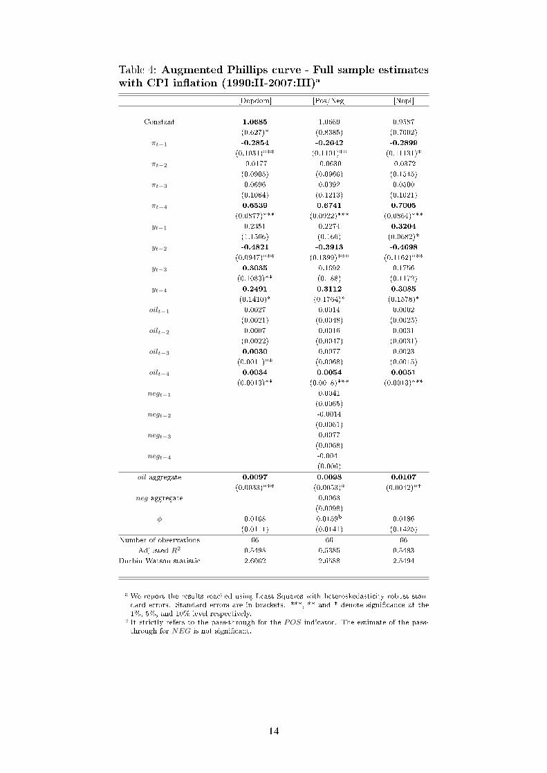
Table 4: Augmented Phillips curve - Full sample estimateswith CPI in�ation (1990:II-2007:III)a


Constant 1.0685 1.0669 0.9587

(0.627)* (0.8385) (0.7002)

πt−1 -0.2854 -0.2642 -0.2899

(0.1031)*** (0.1101)** (0.11131)*

πt−2 -0.0177 -0.0630 -0.0372

(0.0905) (0.0966) (0.1545)

πt−3 0.0696 0.0392 0.0500

(0.1064) (0.1213) (0.1021)

πt−4 0.6539 0.6741 0.7005

(0.0877)*** (0.0922)*** (0.0864)***

yt−1 0.2351 0.2274 0.3204

(1.1566) (0.166) (0.0682)*

yt−2 -0.4821 -0.3913 -0.4698

(0.0947)*** (0.1399)*** (0.1162)***

yt−3 0.3035 0.1692 0.1756

(0.1083)** (0.188) (0.1172)

yt−4 0.2491 0.3112 0.3085

(0.1410)* (0.1764)* (0.1578)*

oilt−1 0.0027 0.0014 0.0002

(0.0021) (0.0048) (0.0025)

oilt−2 0.0007 0.0016 0.0031

(0.0022) (0.0047) (0.0031)

oilt−3 0.0030 0.0077 0.0023

(0.0011)** (0.0068) (0.0015)

oilt−4 0.0034 0.0054 0.0051

(0.0013)** (0.0018)*** (0.0013)***

negt−1 0.0041

(0.0065)

negt−2 -0.0014

(0.0061)

negt−3 0.0077

(0.0068)

negt−4 -0.0041

(0.006)

oil aggregate 0.0097 0.0098 0.0107

(0.0033)*** (0.0053)* (0.0042)**


(0.0098)

φ 0.0168 0.0159b 0.0186

(0.0111) (0.0141) (0.1425)


Adjusted R2 0.5498 0.5385 0.5483




14

5 Potential explanations

How can we explain the decreasing trend in the oil prices-in�ation relationship within the euro

area? Several explanations have been put forward recently, notably by De Gregorio et al.

(2007) and Van den Noord & André (2007). The �rst hypothesis is related to the evolution of

in�ation and the conduct of monetary policy in the euro area. Since the 1970s, it appears that

monetary policy has regained credibility in the pursuit of price stability objectives, thus helping

to anchor in�ation expectations. The fact that interest rates are more responsive to in�ation

nowadays than they were before 1980 may contribute to temper the second-round e�ects from

oil shocks, thereby reducing their in�ationary e�ects and consequently reducing the reaction

from monetary policy.

Other potential explanations for the decline in the oil pass-through are more closely related

to oil. One of the mainstream explanations is the decline in energy intensity of countries

belonging to the euro area. Figure 4 below indeed indicates a declining trend in oil intensity,

i.e. in the ratio of oil consumption over total production (GDP). On the left panel, we report

the evolution since 1981 of a weighted average of oil intensities for several countries belonging

to the EMU: Finland, France, Greece, Italy, the Netherlands, Portugal and Spain11. On the

right panel, we compare the oil intensity in 1981 and 2005 for each of those seven countries.

Oil intensity is expressed in Btu (British thermal unit)12. Those two charts display a lower

dependency to oil in the euro area nowadays, which may explain that EMU members could

face more easily an oil price increase. The weighted average in the euro area indicates that

energy intensity has decreased by 20%, from 8987 barrels in 1980 to 7186 barrels in 2005.

However, this evolution hides a strong degree of heterogeneity between countries, since oil

dependency has fallen by 30% in Finland while it has risen by 36% in Portugal simultaneously.

As Hooker (2002), we investigate this hypothesis empirically by using an alternative indica-

tor for the variation of oil prices (denoted as intoil) in our Phillips curve framework, which is the

quarterly growth rate of the crude oil price weighted by oil intensity. The results are reported in

Table 5, for our two alternative indicators for cyclical positioning, namely the output gap and

the unemployment gap. It appears that the weighted measure of oil prices enters signi�cantly

11See appendix A for further details on the computation of this weighted average.12A British thermal unit is the quantity of heat required to raise the temperature of 1 pound of liquid water

by 1 degree Fahrenheit at the temperature at which water has its greatest density.

15

in the regressions when using the output gap, but it is not the case with the unemployment

gap.

Obviously, the decline in oil intensity mitigates the consequences of oil price shocks on

in�ation. The less capital goods are oil-intensive, the lower production costs and prices of �nal

products will be a�ected by oil price increases. The less consumers buy gasoline, the lower

their purchasing power will be diminished. Moreover, a service-oriented economy (which is

mostly the case of European countries) should be less oil-dependent, and a shock would only

impact a minor component of its production. De Gregorio et al. (2007) highlight that in�ation

in developing countries is more sensitive to oil price shocks mainly because of an old-fashioned

productive structure.

Figure 4: Evolution of oil intensity in the Euro area since 1981

Another explanation refers to the new de�nition of an "oil shock" for the current large and

long-lasting oil price upsurge. The nature of this shock is indeed very di�erent from the two

big oil shocks of the seventies. De Gregorio et al. (2007) and Peterson et al. (2006) point out

this explanation, and Kilian (2006) investigates it empirically using a VAR methodology.

Historical shocks a�ecting oil prices (1974, 1979, 1980) were caused by abrupt oil supply

disruptions on the oil market: the average gross supply shortfalls reached respectively 2.6, 3.5

and 3.3 millions barrels per day13. The left panel of Figure 5 illustrates those collapses for the

world and OPEC oil supplies. On the right panel, we notice that world oil demand follows

closely the direction of the disruption. These shocks were purely exogenous and assimilated as

supply shocks, whereas the current one can be viewed as a demand-driven shock.

13These shocks were often linked and triggered by political events: the Kippour war (1974), the Iranianrevolution (1979) or the Iran-Iraq war (1980), as emphasized by Hamilton (2003).

16

Table 5: Augmented Phillips curve - Oilprices weighted by oil intensity (1990:II-2007:III)a

[Output gap] [Unemployment gap]

Constant 0.2353 0.5504

(0.2663) (0.4250)

πt−1 0.2289 0.3006

(0.1)*** (0.1851)*

πt−2 0.1962 0.07549

(0.0985)*** (0.1851)

πt−3 0.3987 0.2001

(0.1487) (0.1841)

πt−4 -0.0003 0.2652

(0.1142) (0.151)

outputt−1 -0.5090 -7.069

(0.3662) (3.9296)*

outputt−2 0.0290 10.6156

(0.3755) (5.6724)*

outputt−3 -0.8866 -4.6843

(0.5115)* (3.4529)

outputt−4 1.0428 -0.1028

(0.4756)** (2.1627)

intoilt−1 -1.48E-05 -3.97E-05

(0.00003) (0.00004)

intoilt−2 4.69E-05 2.41E-05

(0.00002)** (0.00002)

intoilt−3 6.74E-05 2.00E-05

(0.00002)*** (0.00002)

intoilt−4 -9.00E-07 -1.46E-05

(0.00005) (0.00005)

oil aggregate 9.85E-05 -1.02E-05

(0.00006) (0.000001)

φ 8.47E-04

(0.000717)

Number of observations 97 97

Adjusted R2 0.5800 0.5733

Durbin-Watson statistic 1.8976 1.9789

a We report the results reached using Least Squares withheteroskedasticity-robust standard errors. Standard errors arein brackets. ***, ** and * denote signi�cance at the 1%, 5%,and 10% level respectively. The output variable refers to theoutput gap in the �rst column and to the unemployment gapin the second column.

No major oil supply disruption has occurred since 2001, but world oil demand (widely

in�uenced by the demand coming from emerging countries) has steadily risen. The high oil

prices thus re�ect a disequilibrium between oil supply and oil demand, since the growth rhythm

of supply is insu�cient regarding the evolution of oil demand. OPEC production quotas and

speculative schemes only have impacted marginally the evolution of prices, but have probably

increased their volatility.

17

The implications for in�ation dynamics are speci�c to each oil shock. The smooth current

rise in oil prices may allow agents to adapt their purchases and substitute oil or oil-intensive

production methods with other energy sources and more oil-e�cient capital goods. The rhythm

at which oil prices increase is also rather slow, so that in�ation expectations remain fairly stable,

contributing to price stability. Claims for higher wages have not been very strong since 2001

in the euro area. On the other hand, an abrupt fall in oil supply would generate higher oil

prices and deeply modify relative prices. The perception of in�ation would be disturbed and

may conduct to shifts in consumption habits and pressures for higher wages. Firms would also

translate higher production costs into the price of �nal products.

Figure 5: Evolution of the world oil supply and demand

Finally, several authors provide other explanations for the declining pass-through from oil

prices to headline in�ation. De Gregorio et al. (2007) suggest that the appreciation of the euro

against the U.S. dollar has clearly alleviated the cost of imported goods bought in dollars, such

as oil. They add that the domestic regulation of oil markets has changed since the seventies:

oil markets have become more regulated and may thus be more able to bu�er oil shocks, with

the use of stabilization funds and strategic oil reserves.

18

6 Conclusion

In this paper, we examine the empirical relationship between oil prices and headline in�ation

in the euro area, by estimating an augmented backward-looking Phillips curve since 1970. We

look for nonlinearities using asymmetric oil prices indicators. Potential breakpoints are also

investigated by means of endogenous stability tests (namely Bai/Perron and Andrews/Ploberger

tests).

The estimation results suggest that headline in�ation is a�ected by the variation of oil

prices, and most notably by their increases. A nonlinear pattern in the relationship is thus

reported. However, the established link does not seem to have remained stable over the whole

sample. An identi�ed breakpoint date (1992) allows us to distinguish between two sub-samples

whose estimates display very heterogeneous results. In the second sub-sample, the relationship

clearly weakens, since oil prices do not enter signi�cantly any more in the dynamics of euro

area in�ation.

This paper then investigates two potential explanations: the �rst one is related to a struc-

tural evolution, while the second one is a more short-term and speci�c explanation. On the one

hand, the declining oil intensity (especially noteworthy in the euro area) holds a relevant place

in the increased ability to face oil price increases. On the other hand, it is important to make

the distinction between the current oil price "shock", which is mainly a demand-driven long-

lasting increase, and the big oil shocks of the seventies, that were unexpected sudden shocks

and came from supply disruptions.

Future researches should perform a deeper empirical comparison of those potential expla-

nations for the decline in the pass-through from oil prices to in�ation in the euro area. It

would also be useful to investigate the implications of the nonlinearity and the decline in the

oil price-in�ation linkage within a structural model, paying a particular attention to the role

and consequences for monetary policy. Finally, we should also try to look more carefully at the

transmission channels from oil prices to in�ation, in order to �nd the origin of the asymmetric

feature of the relationship.

19

Appendix A: Data

We work on quarterly data between 1970:I and 2007:III. All the data except oil prices and

exchange rates are extracted from the OECD Economic Outlook database. The variables are

calculated as annualised growth rates.

• Our baseline in�ation indicator is the quarterly growth rate of the seasonally-adjusted

GDP de�ator. The output gap is calculated as the deviation of real GDP from a trend

extracted using the Hodrick-Prescott �lter on the initial series of real GDP, with the

standard quarterly value of 1600 for the smoothing parameter. We also use an in�ation

rate calculated on the basis of the Consumer Price Index (CPI) and an indicator of

unemployment gap (also computed as the deviation of the unemployment rate from a

HP-�ltered trend) to test the robustness of the results in Section 4.

• Oil prices are based on the Brent spot price, which is the most appropriate for European

countries. Data are extracted from the International Energy Agency (IEA) database, and

crude oil prices in U.S. dollars are expressed in domestic currency using the bilateral euro-

dollar (or ECU-dollar) exchange rate from the IMF International Financial Statistics.

� Our baseline indicator (DOPDOM) is therefore the quarterly percentage change in

crude oil prices in domestic currency.

� We also separate the positive (POS) from the negative (NEG) variations of oil

prices to test for asymmetric e�ects on in�ation, as suggested by Mork (1989).

� We �nally calculate the Net Oil Price Increases (NOPI) indicator from Hamilton

(1996). When the oil price level of the current quarter exceeds the value of the

previous year's maximum level, the NOPI is equal to the percentage change between

the two "peaks". For all other values of oil price variations (negative as positive),

the NOPI indicator is equal to zero.

• For the oil intensity indicator used in Section 5, we compute a weighted average of the oil

intensities for six euro area countries for which data are available (Finland, France, Italy,

the Netherlands, Portugal and Spain). The weights are related to the consumption share

of each country in total oil consumption for those six countries. Since oil intensity data

are only yearly (from 1980 to 2005), we keep the same value for the four quarters of each

year.

20

References

Andrews, Donald W.K. (1993): �Tests for Parameter Instability and Structural Change withUnknown Change Point�, Econometrica, vol. 61, no. 4, pp. 821�856.

Andrews, Donald W.K. & Ploberger, Werner (1994): �Optimal Tests When a NuisanceParameter is Present Only under the Alternative�, Econometrica, vol. 62, no. 6, pp. 1383�1414.

Bai, Jushan & Perron, Pierre (1998): �Estimating and Testing Linear Models with MultipleStructural Changes�, Econometrica, vol. 66, no. 1, pp. 47�78.

Blanchard, Olivier J. &Gali, Jordi (2007): �The Macroeconomic E�ects of Oil Price Shocks:Why are the 2000s so di�erent from the 1970s?�, NBER Working Paper 13368, NationalBureau of Economic Research.

Borio, Claudio & Filardo, Andrew (2007): �Globalisation and In�ation: New Cross-countryEvidence on the Global Determinants of Domestic In�ation�, BIS Working Paper 227, Bankfor International Settlements, 54 p.

Brayton, Flint, Roberts, John M. &Williams, John C. (1999): �What's Happened to thePhillips Curve?�, Finance and Economics Discussion Series 1999-49, Board of Governors ofthe Federal Reserve System, 39 p.

De Gregorio, José, Landerretche, Oscar & Neilson, Christopher (2007): �Another Pass-Through Bites the Dust? Oil Prices and In�ation�, Economia, vol. 7, no. 2, pp. 155�208.

Fuhrer, Je�rey C. (1995): �The Phillips Cuve is Alive and Well�, New England EconomicReview, , no. March/April, pp. 41�56.

Hamilton, James D. (1996): �This is What Happened to the Oil Price-Macroeconomy Rela-tionship�, Journal of Monetary Economics, vol. 38, no. 2, pp. 215�220.

Hamilton, James D. (2003): �What is an Oil Shock?�, Journal of Econometrics, vol. 113,no. 2, pp. 363�398.

Hooker, Mark A. (2002): �Are Oil Shocks In�ationary? Asymmetric and Nonlinear Speci�-cations versus Changes in Regime�, Journal of Money, Credit and Banking., vol. 34, no. 2,pp. 540�561.

Kilian, Lutz (2006): �Not All Oil Price Shocks Are Alike: Disentangling Demand and SupplyShocks in the Crude Oil Market�, CEPR Discussion Paper 5994, Center for Economic PolicyResearch.

LeBlanc, Michael & Chinn, Menzie D. (2004): �Do High Oil Prices Presage In�ation? TheEvidence from G-5 Countries�, Working Paper 1021, Santa Cruz Center for InternationalEconomics.

Mork, Knut A. (1989): �Oil and the Macroeconomy When Prices Go Up and Down: AnExtension of Hamilton's Results�, Journal of Political Economy, vol. 97, no. 3, pp. 740�744.

Mork, Knut A., Olsen, Oystein & Mysen, Hans T. (1994): �Macroeconomic Responses toOil Price Increases and Decreases in Seven OECD Countries�, The Energy Journal, vol. 15,no. 4, pp. 19�35.

21

Mory, Javier F. (1993): �Oil Prices and Economic Activity: Is the Relationship Symmetric?�,The Energy Journal, vol. 14, no. 4, pp. 151�161.

Peterson, John, Farmer, Richard, Lasky, Mark, Mascaro, Angelo & Weber, Adam(2006): �The Economic E�ects of Recent Increases in Energy Prices�, CBO Paper 2835,Congress of the United States - Congressional Budget O�ce, 36 p.

Van den Noord, Paul & André, Christophe (2007): �Why Has Core In�ation Remained soMuted in the Face of Oil Shocks?�, Economics Department Working Paper 551, OECD, 35p.

22

cinquiemes doctoriales de macrofi et seminaire...

Documents