CircuiTikZversion 0.8.3 (2017/05/28)

Massimo A. Redaelli (m.redaelli@gmail.com)Stefan Lindner (stefan.lindner@fau.de)Stefan Erhardt (stefan.erhardt@fau.de)

May 28, 2017

Contents1 Introduction 3

1.1 About . . . . . . . . . . . . . . . . . . . . . . . . . . . . . . . . . . . . . . . . . . . 31.2 Loading the package . . . . . . . . . . . . . . . . . . . . . . . . . . . . . . . . . . . 31.3 Requirements . . . . . . . . . . . . . . . . . . . . . . . . . . . . . . . . . . . . . . . 31.4 Incompatible packages . . . . . . . . . . . . . . . . . . . . . . . . . . . . . . . . . . 31.5 License . . . . . . . . . . . . . . . . . . . . . . . . . . . . . . . . . . . . . . . . . . . 31.6 Feedback . . . . . . . . . . . . . . . . . . . . . . . . . . . . . . . . . . . . . . . . . 4

2 Incompabilities between version 4

3 Package options 4

4 The components 64.1 Monopoles . . . . . . . . . . . . . . . . . . . . . . . . . . . . . . . . . . . . . . . . . 74.2 Bipoles . . . . . . . . . . . . . . . . . . . . . . . . . . . . . . . . . . . . . . . . . . . 9

4.2.1 Instruments . . . . . . . . . . . . . . . . . . . . . . . . . . . . . . . . . . . . 94.2.2 Basic resistive bipoles . . . . . . . . . . . . . . . . . . . . . . . . . . . . . . 94.2.3 Resistors and the like . . . . . . . . . . . . . . . . . . . . . . . . . . . . . . 104.2.4 Diodes and such . . . . . . . . . . . . . . . . . . . . . . . . . . . . . . . . . 114.2.5 Other tripole-like diodes . . . . . . . . . . . . . . . . . . . . . . . . . . . . . 144.2.6 Basic dynamical bipoles . . . . . . . . . . . . . . . . . . . . . . . . . . . . . 154.2.7 Stationary sources . . . . . . . . . . . . . . . . . . . . . . . . . . . . . . . . 174.2.8 Sinusoidal sources . . . . . . . . . . . . . . . . . . . . . . . . . . . . . . . . 184.2.9 Special sources . . . . . . . . . . . . . . . . . . . . . . . . . . . . . . . . . . 184.2.10 DC sources . . . . . . . . . . . . . . . . . . . . . . . . . . . . . . . . . . . . 184.2.11 Mechanical Analogy . . . . . . . . . . . . . . . . . . . . . . . . . . . . . . . 194.2.12 Switch . . . . . . . . . . . . . . . . . . . . . . . . . . . . . . . . . . . . . . . 194.2.13 Block diagram components . . . . . . . . . . . . . . . . . . . . . . . . . . . 20

4.3 Tripoles . . . . . . . . . . . . . . . . . . . . . . . . . . . . . . . . . . . . . . . . . . 224.3.1 Controlled sources . . . . . . . . . . . . . . . . . . . . . . . . . . . . . . . . 224.3.2 Transistors . . . . . . . . . . . . . . . . . . . . . . . . . . . . . . . . . . . . 234.3.3 Electronic Tubes . . . . . . . . . . . . . . . . . . . . . . . . . . . . . . . . . 274.3.4 Block diagram . . . . . . . . . . . . . . . . . . . . . . . . . . . . . . . . . . 274.3.5 Switch . . . . . . . . . . . . . . . . . . . . . . . . . . . . . . . . . . . . . . . 284.3.6 Electro-Mechanical Devices . . . . . . . . . . . . . . . . . . . . . . . . . . . 28

4.4 Double bipoles . . . . . . . . . . . . . . . . . . . . . . . . . . . . . . . . . . . . . . 29

1

4.5 Logic gates . . . . . . . . . . . . . . . . . . . . . . . . . . . . . . . . . . . . . . . . 304.5.1 American Logic gates . . . . . . . . . . . . . . . . . . . . . . . . . . . . . . 304.5.2 European Logic gates . . . . . . . . . . . . . . . . . . . . . . . . . . . . . . 31

4.6 Amplifiers . . . . . . . . . . . . . . . . . . . . . . . . . . . . . . . . . . . . . . . . . 324.7 Support shapes . . . . . . . . . . . . . . . . . . . . . . . . . . . . . . . . . . . . . . 33

5 Usage 345.1 Labels and Annotations . . . . . . . . . . . . . . . . . . . . . . . . . . . . . . . . . 345.2 Currents . . . . . . . . . . . . . . . . . . . . . . . . . . . . . . . . . . . . . . . . . . 355.3 Flows . . . . . . . . . . . . . . . . . . . . . . . . . . . . . . . . . . . . . . . . . . . 375.4 Voltages . . . . . . . . . . . . . . . . . . . . . . . . . . . . . . . . . . . . . . . . . . 38

5.4.1 European style . . . . . . . . . . . . . . . . . . . . . . . . . . . . . . . . . . 385.4.2 American style . . . . . . . . . . . . . . . . . . . . . . . . . . . . . . . . . . 39

5.5 Nodes . . . . . . . . . . . . . . . . . . . . . . . . . . . . . . . . . . . . . . . . . . . 395.6 Special components . . . . . . . . . . . . . . . . . . . . . . . . . . . . . . . . . . . . 415.7 Integration with siunitx . . . . . . . . . . . . . . . . . . . . . . . . . . . . . . . . 425.8 Mirroring and Inverting . . . . . . . . . . . . . . . . . . . . . . . . . . . . . . . . . 435.9 Putting them together . . . . . . . . . . . . . . . . . . . . . . . . . . . . . . . . . . 435.10 Line joins between Path Components . . . . . . . . . . . . . . . . . . . . . . . . . . 44

6 Not only bipoles 446.1 Anchors . . . . . . . . . . . . . . . . . . . . . . . . . . . . . . . . . . . . . . . . . . 44

6.1.1 Logical ports . . . . . . . . . . . . . . . . . . . . . . . . . . . . . . . . . . . 446.1.2 Transistors . . . . . . . . . . . . . . . . . . . . . . . . . . . . . . . . . . . . 456.1.3 Other tripoles . . . . . . . . . . . . . . . . . . . . . . . . . . . . . . . . . . . 466.1.4 Operational amplifier . . . . . . . . . . . . . . . . . . . . . . . . . . . . . . 476.1.5 Double bipoles . . . . . . . . . . . . . . . . . . . . . . . . . . . . . . . . . . 48

6.2 Input arrows . . . . . . . . . . . . . . . . . . . . . . . . . . . . . . . . . . . . . . . 496.3 Labels and custom twoport boxes . . . . . . . . . . . . . . . . . . . . . . . . . . . . 506.4 Box option . . . . . . . . . . . . . . . . . . . . . . . . . . . . . . . . . . . . . . . . 506.5 Dash optional parts . . . . . . . . . . . . . . . . . . . . . . . . . . . . . . . . . . . 506.6 Transistor paths . . . . . . . . . . . . . . . . . . . . . . . . . . . . . . . . . . . . . 50

7 Customization 517.1 Parameters . . . . . . . . . . . . . . . . . . . . . . . . . . . . . . . . . . . . . . . . 517.2 Components size . . . . . . . . . . . . . . . . . . . . . . . . . . . . . . . . . . . . . 527.3 Colors . . . . . . . . . . . . . . . . . . . . . . . . . . . . . . . . . . . . . . . . . . . 53

8 FAQ 55

9 Examples 55

10 Changelog 61

Index of the components 66

2

1 Introduction1.1 AboutCircuiTikZ was initiated by Massimo Redaelli in 2007, who was working as a research assistantat the Polytechnic University of Milan, Italy, and needed a tool for creating exercises and exams.After he left University in 2010 the development of CircuiTikZ slowed down, since LATEX is mainlyestablished in the academic world. In 2015 Stefan Lindner and Stefan Erhardt, both working asresearch assistants at the University of Erlangen-Nürnberg, Germany, joined the team and nowmaintain the project together with the initial author.

The use of CircuiTikZ is, of course, not limited to academic teaching. The package gets widelyused by engineers for typesetting electronic circuits for articles and publications all over the world.

This documentation is somewhat scant. Hopefully the authors will find the leisure to improveit some day.

1.2 Loading the package

LATEX ConTEXt1

\usepackagecircuitikz \usemodule[circuitikz]

TikZ will be automatically loaded.CircuiTikZ commands are just TikZ commands, so a minimum usage example would be:

R11\tikz \draw (0,0) to[R=$R_1$] (2,0);

1.3 Requirements• tikz, version ≥ 3;

• xstring, not older than 2009/03/13;

• siunitx, if using siunitx option.

1.4 Incompatible packagesTikZ’s own circuit library, which is based on CircuiTikZ, (re?)defines several styles used by thislibrary. In order to have them work together you can use the compatibility package option,which basically prefixes the names of all CircuiTikZ to[] styles with an asterisk.

So, if loaded with said option, one must write (0,0) to[*R] (2,0) and, for transistors on apath, (0,0) to[*Tnmos] (2,0), and so on (but (0,0) node[nmos] ). See example at page 61.

1.5 LicenseCopyright © 2007–2017 Massimo Redaelli. This package is author-maintained. Permission isgranted to copy, distribute and/or modify this software under the terms of the LATEX ProjectPublic License, version 1.3.1, or the GNU Public License. This software is provided ‘as is’, withoutwarranty of any kind, either expressed or implied, including, but not limited to, the impliedwarranties of merchantability and fitness for a particular purpose.

1ConTEXt support was added mostly thanks to Mojca Miklavec and Aditya Mahajan.

3

1.6 FeedbackThe easiest way to contact the authors is via the official Github repository: https://github.com/circuitikz/circuitikz/issues

2 Incompabilities between versionHere, we will provide a list of incompabilitys between different version of circuitikz. We will tryto hold this list short, but sometimes it is easier to break with old syntax than including a lot ofswitches and compatibility layers. You can check the used version at your local installation usingthe macro \pgfcircversion.

• Since v0.8.2: voltage and current label directions(v<= / i<=) do NOT change the orienta-tion of the drawn source shape anymore. Use the ”invert” option to rotate the shape of thesource. Furthermore, from this version on, the current label(i=) at current sources can beused independent of the regular label(l=).

• Since v0.7?: The label behaviour at mirrored bipoles has changes, this fixes the voltagedrawing, but perhaps you have to adjust your label positions.

• Since v0.5.1: The parts pfet,pigfete,pigfetebulk and pigfetd are now mirrored by default.Please adjust your yscale-option to correct this.

• Since v0.5: New voltage counting direction, here exists an option to use the old behaviour

For older projects, you can use an older version locally using the git-version and picking the correctcommit from the repository (branch gh-pages).

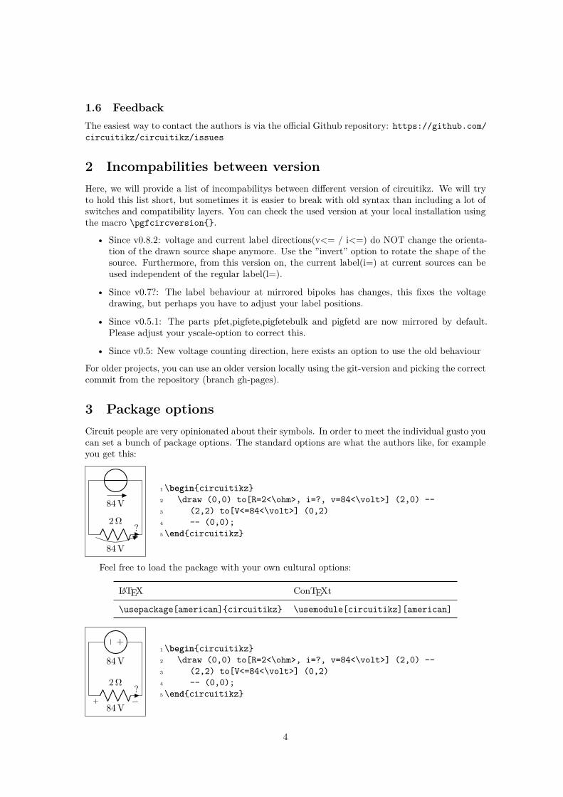
3 Package optionsCircuit people are very opinionated about their symbols. In order to meet the individual gusto youcan set a bunch of package options. The standard options are what the authors like, for exampleyou get this:

2Ω

84V

?

84V1\begincircuitikz2 \draw (0,0) to[R=2<\ohm>, i=?, v=84<\volt>] (2,0) --3 (2,2) to[V<=84<\volt>] (0,2)4 -- (0,0);5\endcircuitikz

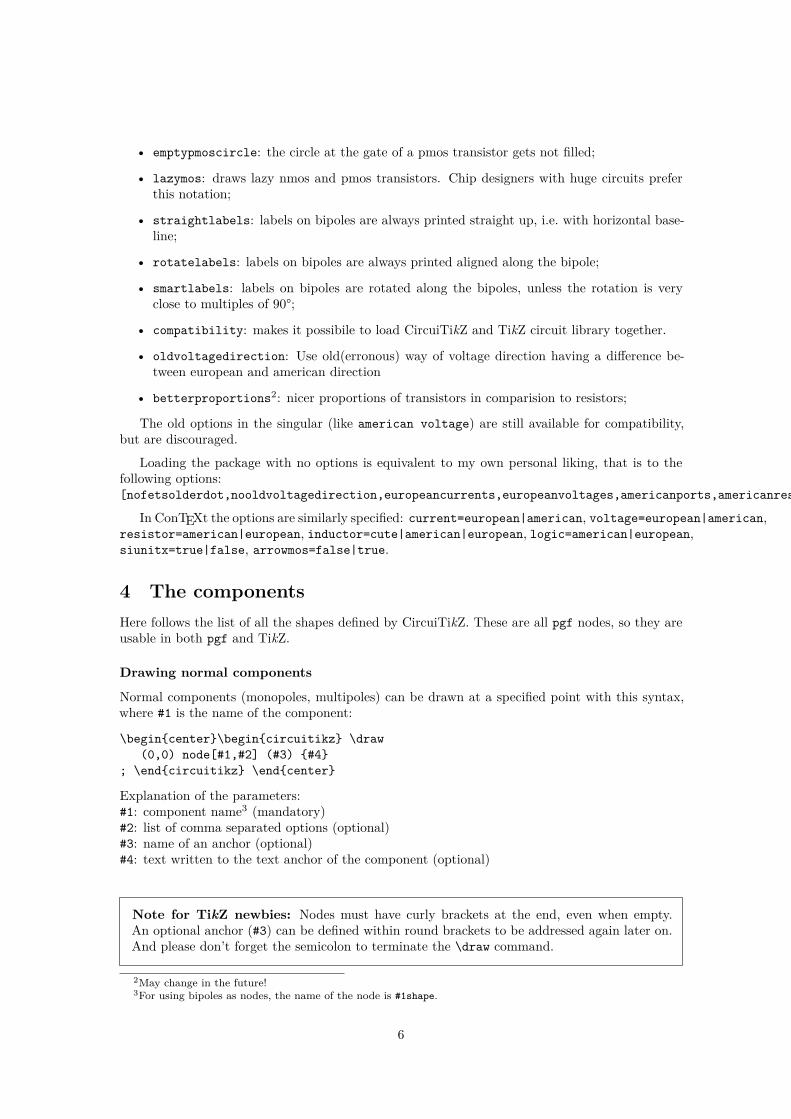
Feel free to load the package with your own cultural options:

LATEX ConTEXt

\usepackage[american]circuitikz \usemodule[circuitikz][american]

2Ω

+ −84V

?

− +

84V1\begincircuitikz2 \draw (0,0) to[R=2<\ohm>, i=?, v=84<\volt>] (2,0) --3 (2,2) to[V<=84<\volt>] (0,2)4 -- (0,0);5\endcircuitikz

4

Here is the list of all the options:

• europeanvoltages: uses arrows to define voltages, and uses european-style voltage sources;

• straightvoltages: uses arrows to define voltages, and and uses straight voltage arrows;

• americanvoltages: uses − and + to define voltages, and uses american-style voltage sources;

• europeancurrents: uses european-style current sources;

• americancurrents: uses american-style current sources;

• europeanresistors: uses rectangular empty shape for resistors, as per european standards;

• americanresistors: uses zig-zag shape for resistors, as per american standards;

• europeaninductors: uses rectangular filled shape for inductors, as per european standards;

• americaninductors: uses ”4-bumps” shape for inductors, as per american standards;

• cuteinductors: uses my personal favorite, ”pig-tailed” shape for inductors;

• americanports: uses triangular logic ports, as per american standards;

• europeanports: uses rectangular logic ports, as per european standards;

• americangfsurgearrester: uses round gas filled surge arresters, as per american standards;

• europeangfsurgearrester: uses rectangular gas filled surge arresters, as per europeanstandards;

• european: equivalent to europeancurrents, europeanvoltages, europeanresistors, europeaninductors,europeanports, europeangfsurgearrester;

• american: equivalent to americancurrents, americanvoltages, americanresistors, americaninductors,americanports, americangfsurgearrester;

• siunitx: integrates with SIunitx package. If labels, currents or voltages are of the form#1<#2> then what is shown is actually \SI#1#2;

• nosiunitx: labels are not interpreted as above;

• fulldiode: the various diodes are drawn and filled by default, i.e. when using styles suchas diode, D, sD, …Other diode styles can always be forced with e.g. Do, D-, …

• strokediode: the various diodes are drawn and stroke by default, i.e. when using stylessuch as diode, D, sD, …Other diode styles can always be forced with e.g. Do, D*, …

• emptydiode: the various diodes are drawn but not filled by default, i.e. when using stylessuch as D, sD, …Other diode styles can always be forced with e.g. Do, D-, …

• arrowmos: pmos and nmos have arrows analogous to those of pnp and npn transistors;

• noarrowmos: pmos and nmos do not have arrows analogous to those of pnp and npn tran-sistors;

• fetbodydiode: draw the body diode of a FET;

• nofetbodydiode: do not draw the body diode of a FET;

• fetsolderdot: draw solderdot at bulk-source junction of some transistors;

• nofetsolderdot: do not draw solderdot at bulk-source junction of some transistors;

5

• emptypmoscircle: the circle at the gate of a pmos transistor gets not filled;

• lazymos: draws lazy nmos and pmos transistors. Chip designers with huge circuits preferthis notation;

• straightlabels: labels on bipoles are always printed straight up, i.e. with horizontal base-line;

• rotatelabels: labels on bipoles are always printed aligned along the bipole;

• smartlabels: labels on bipoles are rotated along the bipoles, unless the rotation is veryclose to multiples of 90°;

• compatibility: makes it possibile to load CircuiTikZ and TikZ circuit library together.

• oldvoltagedirection: Use old(erronous) way of voltage direction having a difference be-tween european and american direction

• betterproportions2: nicer proportions of transistors in comparision to resistors;

The old options in the singular (like american voltage) are still available for compatibility,but are discouraged.

Loading the package with no options is equivalent to my own personal liking, that is to thefollowing options:[nofetsolderdot,nooldvoltagedirection,europeancurrents,europeanvoltages,americanports,americanresistors,cuteinductors,europeangfsurgearrester,nosiunitx,noarrowmos,smartlabels,nocompatibility].

In ConTEXt the options are similarly specified: current=european|american, voltage=european|american,resistor=american|european, inductor=cute|american|european, logic=american|european,siunitx=true|false, arrowmos=false|true.

4 The componentsHere follows the list of all the shapes defined by CircuiTikZ. These are all pgf nodes, so they areusable in both pgf and TikZ.

Drawing normal components

Normal components (monopoles, multipoles) can be drawn at a specified point with this syntax,where #1 is the name of the component:

\begincenter\begincircuitikz \draw(0,0) node[#1,#2] (#3) #4

; \endcircuitikz \endcenter

Explanation of the parameters:#1: component name3 (mandatory)#2: list of comma separated options (optional)#3: name of an anchor (optional)#4: text written to the text anchor of the component (optional)

Note for TikZ newbies: Nodes must have curly brackets at the end, even when empty.An optional anchor (#3) can be defined within round brackets to be addressed again later on.And please don’t forget the semicolon to terminate the \draw command.

2May change in the future!3For using bipoles as nodes, the name of the node is #1shape.

6

Drawing bipoles/two-ports

Bipoles/Two-ports (plus some special components) can be drawn between two points using thefollowing command:

\begincenter\begincircuitikz \draw(0,0) to[#1,#2] (2,0)

; \endcircuitikz \endcenter

Explanation of the parameters:#1: component name (mandatory)#2: list of comma separated options (optional)Transistors and some other components can also be placed using the syntax for bipoles. Seesection 6.6.

If using the \tikzexternalize feature, as of Tikz 2.1 all pictures must end with\endtikzpicture. Thus you cannot use the circuitikz environment.

Which is ok: just use the environment tikzpicture: everything will work there just fine.

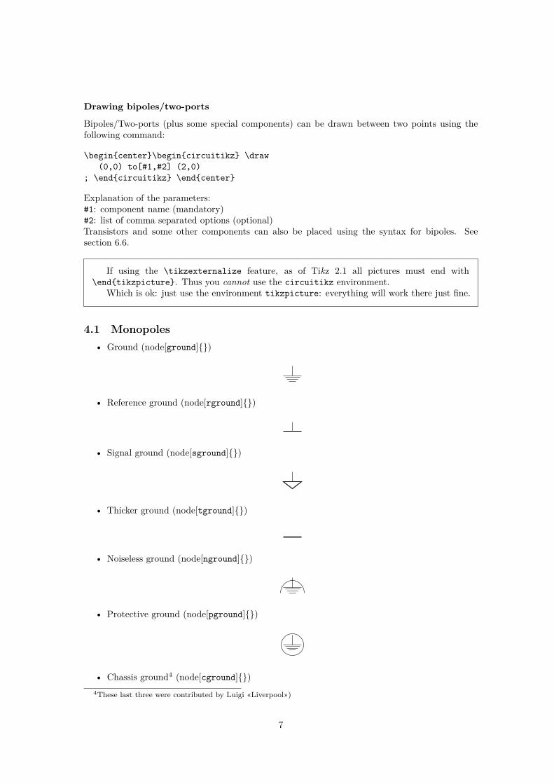
4.1 Monopoles• Ground (node[ground])

• Reference ground (node[rground])

• Signal ground (node[sground])

• Thicker ground (node[tground])

• Noiseless ground (node[nground])

• Protective ground (node[pground])

• Chassis ground4 (node[cground])4These last three were contributed by Luigi «Liverpool»)

7

• Antenna (node[antenna])

• Receiving antenna (node[rxantenna])

• Transmitting antenna (node[txantenna])

• Transmission line stub (node[tlinestub])

• VCC/VDD (node[vcc])

• VEE/VSS (node[vee])

• match (node[match])

8

4.2 Bipoles4.2.1 Instruments

• Ammeter (ammeter)

A

• Voltmeter (voltmeter)

V

• Ohmmeter (ohmmeter)

Ω

4.2.2 Basic resistive bipoles

• Short circuit (short)

• Open circuit (open)

• Lamp (lamp)

• Generic (symmetric) bipole (generic)

• Tunable generic bipole (tgeneric)

• Generic asymmetric bipole (ageneric)

• Generic asymmetric bipole (full) (fullgeneric)

9

• Tunable generic bipole (full) (tfullgeneric)

• Memristor (memristor, or Mr)

4.2.3 Resistors and the like

If (default behaviour) americanresistors option is active (or the style [american resistors]is used), the resistor is displayed as follows:

• Resistor (R, or american resistor)

• Variable resistor (vR, or variable american resistor)

• Potentiometer (pR, or american potentiometer)

If instead europeanresistors option is active (or the style [european resistors] is used),the resistors, variable resistors and potentiometers are displayed as follows:

• Resistor (R, or european resistor)

• Variable resistor (vR, or european variable resistor)

• Potentiometer (pR, or european potentiometer)

Other miscellaneous resistor-like devices:

• Varistor (varistor)

U

10

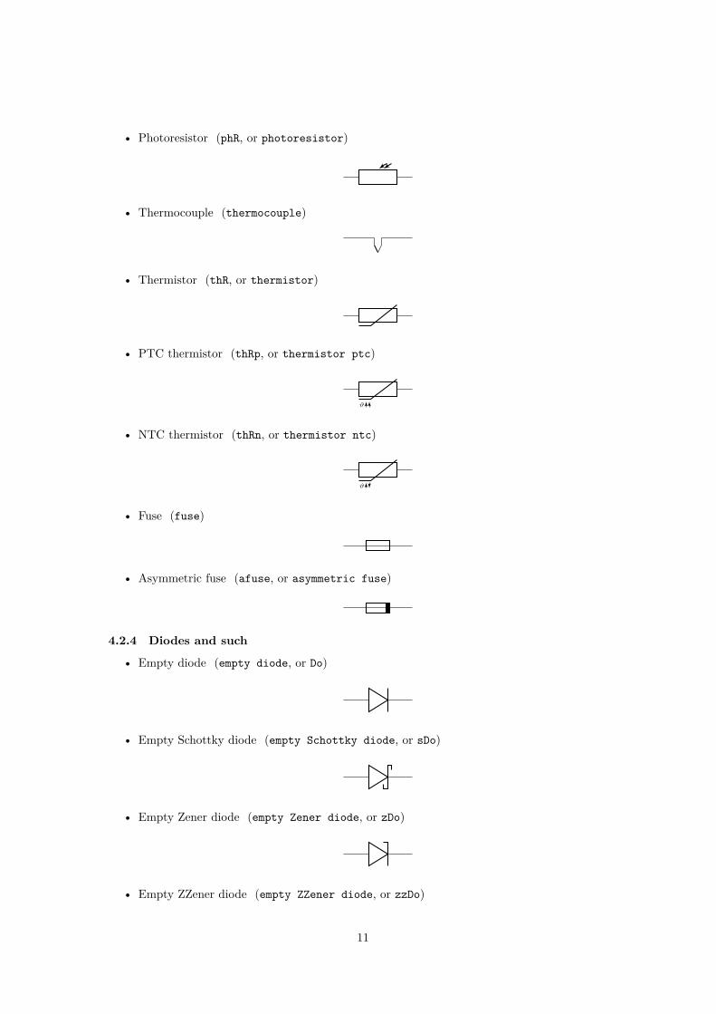
• Photoresistor (phR, or photoresistor)

• Thermocouple (thermocouple)

• Thermistor (thR, or thermistor)

• PTC thermistor (thRp, or thermistor ptc)

ϑ

• NTC thermistor (thRn, or thermistor ntc)

ϑ

• Fuse (fuse)

• Asymmetric fuse (afuse, or asymmetric fuse)

4.2.4 Diodes and such

• Empty diode (empty diode, or Do)

• Empty Schottky diode (empty Schottky diode, or sDo)

• Empty Zener diode (empty Zener diode, or zDo)

• Empty ZZener diode (empty ZZener diode, or zzDo)

11

• Empty tunnel diode (empty tunnel diode, or tDo)

• Empty photodiode (empty photodiode, or pDo)

• Empty led (empty led, or leDo)

• Empty varcap (empty varcap, or VCo)

• Full diode (full diode, or D*)

• Full Schottky diode (full Schottky diode, or sD*)

• Full Zener diode (full Zener diode, or zD*)

• Full ZZener diode (full ZZener diode, or zzD*)

• Full tunnel diode (full tunnel diode, or tD*)

• Full photodiode (full photodiode, or pD*)

12

• Full led (full led, or leD*)

• Full varcap (full varcap, or VC*)

• Stroke diode (stroke diode, or D-)

• Stroke Schottky diode (stroke Schottky diode, or sD-)

• Stroke Zener diode (stroke Zener diode, or zD-)

• Stroke ZZener diode (stroke ZZener diode, or zzD-)

• Stroke tunnel diode (stroke tunnel diode, or tD-)

• Stroke photodiode (stroke photodiode, or pD-)

• Stroke led (stroke led, or leD-)

• Stroke varcap (stroke varcap, or VC-)

13

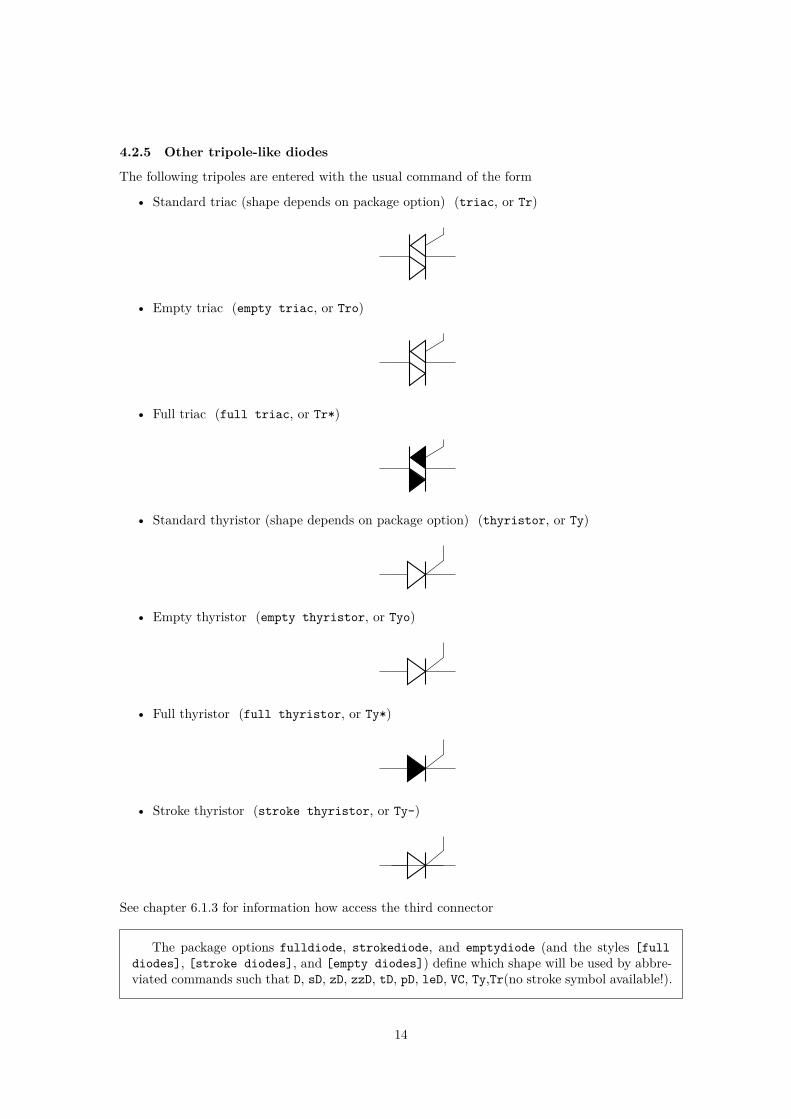
4.2.5 Other tripole-like diodes

The following tripoles are entered with the usual command of the form

• Standard triac (shape depends on package option) (triac, or Tr)

• Empty triac (empty triac, or Tro)

• Full triac (full triac, or Tr*)

• Standard thyristor (shape depends on package option) (thyristor, or Ty)

• Empty thyristor (empty thyristor, or Tyo)

• Full thyristor (full thyristor, or Ty*)

• Stroke thyristor (stroke thyristor, or Ty-)

See chapter 6.1.3 for information how access the third connector

The package options fulldiode, strokediode, and emptydiode (and the styles [fulldiodes], [stroke diodes], and [empty diodes]) define which shape will be used by abbre-viated commands such that D, sD, zD, zzD, tD, pD, leD, VC, Ty,Tr(no stroke symbol available!).

14

• Squid (squid)

• Barrier (barrier)

• European gas filled surge arrester (european gas filled surge arrester)

• American gas filled surge arrester (american gas filled surge arrester)

If (default behaviour) europeangfsurgearrester option is active (or the style [europeangas filled surge arrester] is used), the shorthands gas filled surge arrester andgf surge arrester are equivalent to the european version of the component.

If otherwise americangfsurgearrester option is active (or the style [american gasfilled surge arrester] is used), the shorthands the shorthands gas filled surgearrester and gf surge arrester are equivalent to the american version of the component.

4.2.6 Basic dynamical bipoles

• Capacitor (capacitor, or C)

• Polar capacitor (polar capacitor, or pC)

• Electrolytic capacitor (ecapacitor, or eC,elko)

+

• Variable capacitor (variable capacitor, or vC)

• Piezoelectric Element (piezoelectric, or PZ)

15

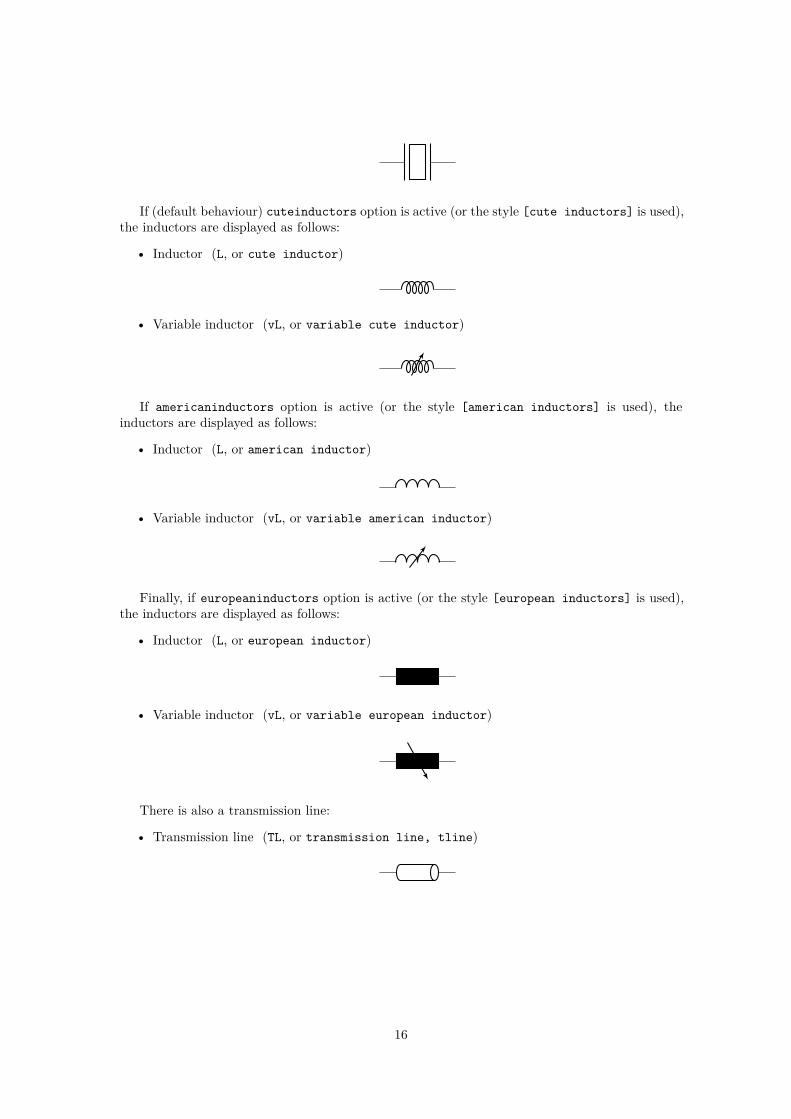
If (default behaviour) cuteinductors option is active (or the style [cute inductors] is used),the inductors are displayed as follows:

• Inductor (L, or cute inductor)

• Variable inductor (vL, or variable cute inductor)

If americaninductors option is active (or the style [american inductors] is used), theinductors are displayed as follows:

• Inductor (L, or american inductor)

• Variable inductor (vL, or variable american inductor)

Finally, if europeaninductors option is active (or the style [european inductors] is used),the inductors are displayed as follows:

• Inductor (L, or european inductor)

• Variable inductor (vL, or variable european inductor)

There is also a transmission line:

• Transmission line (TL, or transmission line, tline)

16

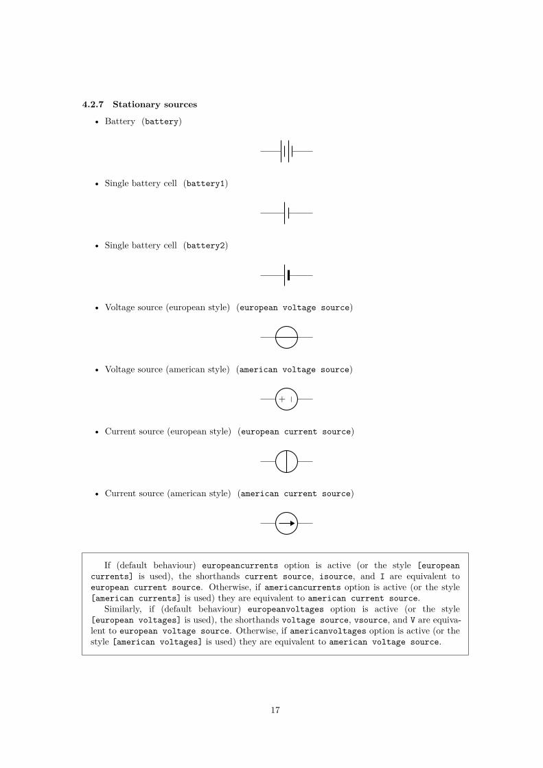
4.2.7 Stationary sources

• Battery (battery)

• Single battery cell (battery1)

• Single battery cell (battery2)

• Voltage source (european style) (european voltage source)

• Voltage source (american style) (american voltage source)

−+

• Current source (european style) (european current source)

• Current source (american style) (american current source)

If (default behaviour) europeancurrents option is active (or the style [europeancurrents] is used), the shorthands current source, isource, and I are equivalent toeuropean current source. Otherwise, if americancurrents option is active (or the style[american currents] is used) they are equivalent to american current source.

Similarly, if (default behaviour) europeanvoltages option is active (or the style[european voltages] is used), the shorthands voltage source, vsource, and V are equiva-lent to european voltage source. Otherwise, if americanvoltages option is active (or thestyle [american voltages] is used) they are equivalent to american voltage source.

17

4.2.8 Sinusoidal sources

Here because I was asked for them. But how do you distinguish one from the other?!• Sinusoidal voltage source (sinusoidal voltage source, or vsourcesin, sV)

• Sinusoidal current source (sinusoidal current source, or isourcesin, sI)

4.2.9 Special sources

• Square voltage source (square voltage source, or vsourcesquare, sqV)

• Triangle voltage source (vsourcetri, or tV)

• Empty voltage source (esource)

• Photovoltaic-voltage source (pvsource)

• Double Zero style current source (ioosource)

• Double Zero style voltage source (voosource)

4.2.10 DC sources

• DC voltage source (dcvsource)

• DC current source (dcisource)

18

4.2.11 Mechanical Analogy

• Mechanical Damping (damper)

• Mechanical Stiffness (spring)

• Mechanical Mass (mass)

4.2.12 Switch

• Switch (switch, or spst)

• Closing switch (closing switch, or cspst)

• Opening switch (opening switch, or ospst)

• Normally open switch (normal open switch, or nos)

• Normally closed switch (normal closed switch, or ncs)

• Push button (push button)

19

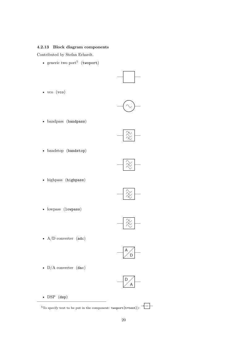
4.2.13 Block diagram components

Contributed by Stefan Erhardt.

• generic two port5 (twoport)

• vco (vco)

• bandpass (bandpass)

• bandstop (bandstop)

• highpass (highpass)

• lowpass (lowpass)

• A/D converter (adc)

AD

• D/A converter (dac)

DA

• DSP (dsp)

5To specify text to be put in the component: twoport[t=text]):text

20

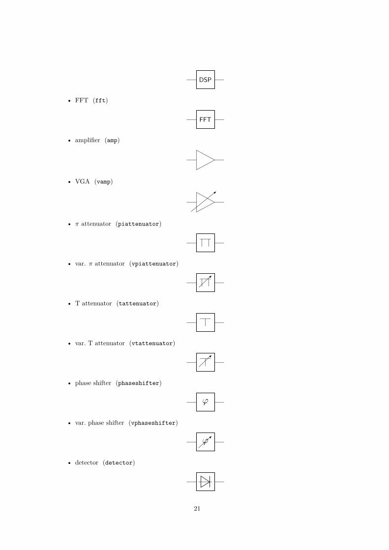
DSP

• FFT (fft)

FFT

• amplifier (amp)

• VGA (vamp)

• π attenuator (piattenuator)

• var. π attenuator (vpiattenuator)

• T attenuator (tattenuator)

• var. T attenuator (vtattenuator)

• phase shifter (phaseshifter)

φ

• var. phase shifter (vphaseshifter)

φ

• detector (detector)

21

4.3 Tripoles4.3.1 Controlled sources

Admittedly, graphically they are bipoles. But I couldn’t…

• Controlled voltage source (european style) (european controlled voltage source)

• Controlled voltage source (american style) (american controlled voltage source)

−+• Controlled current source (european style) (european controlled current source)

• Controlled current source (american style) (american controlled current source)

If (default behaviour) europeancurrents option is active (or the style [europeancurrents] is used), the shorthands controlled current source, cisource, and cI areequivalent to european controlled current source. Otherwise, if americancurrents op-tion is active (or the style [american currents] is used) they are equivalent to americancontrolled current source.

Similarly, if (default behaviour) europeanvoltages option is active (or the style[european voltages] is used), the shorthands controlled voltage source, cvsource,and cV are equivalent to european controlled voltage source. Otherwise, ifamericanvoltages option is active (or the style [american voltages] is used) they areequivalent to american controlled voltage source.

• Controlled sinusoidal voltage source (controlled sinusoidal voltage source, or controlledvsourcesin, cvsourcesin, csV)

• Controlled sinusoidal current source (controlled sinusoidal current source, or controlledisourcesin, cisourcesin, csI)

22

4.3.2 Transistors

• nmos (node[nmos])

• pmos (node[pmos])

• npn (node[npn])

• pnp (node[pnp])

• npn (node[npn,photo])

• pnp (node[pnp,photo])

• nigbt (node[nigbt])

• pigbt (node[pigbt])

23

• Lnigbt (node[Lnigbt])

• Lpigbt (node[Lpigbt])

For all transistors a bodydiode(or freewheeling diode) can automatically be drawn. Just usethe global option bodydiode, or for single transistors, the tikz-option bodydiode:

1\begincircuitikz2 \draw (0,0) node[npn,bodydiode](npn)++(2,0)node[pnp,

bodydiode](npn);3 \draw (0,-2) node[nigbt,bodydiode](npn)++(2,0)node[

pigbt,bodydiode](npn);4 \draw (0,-4) node[nfet,bodydiode](npn)++(2,0)node[

pfet,bodydiode](npn);5\endcircuitikz

The Base/Gate connection of all transistors can be disable by using the options nogate ornobase, respectively. The Base/Gate anchors are floating, but there an additional anchor ”no-gate”/”nobase”, which can be used to point to the unconnected base:

E

C

B

1\begincircuitikz2 \draw (2,0) node[npn,nobase](npn);3 \draw (npn.E) node[below]E;4 \draw (npn.C) node[above]C;5 \draw (npn.B) node[circ] node[left]B;6 \draw[dashed,red,-latex] (1,0.5)--(npn.nobase);7\endcircuitikz

If the option arrowmos is used (or after the command \ctikzsettripoles/mos style/arrowsis given), this is the output:

• nmos (node[nmos])

24

• pmos (node[pmos])

To draw the PMOS circle non-solid, use the option emptycircle or the command \ctikzsettripoles/pmos style/emptycircle.

• pmos (node[pmos,emptycircle])

nfets and pfets have been incorporated based on code provided by Clemens Helfmeier andTheodor Borsche. Use the package options fetsolderdot/nofetsolderdot to enable/disablesolderdot at some fet-transistors. Additionally, the solderdot option can be enabled/disabled forsingle transistors with the option ”solderdot” and ”nosolderdot”, respectively.

• nfet (node[nfet])

• nigfete (node[nigfete])

• nigfete (node[nigfete,solderdot])

• nigfetebulk (node[nigfetebulk])

25

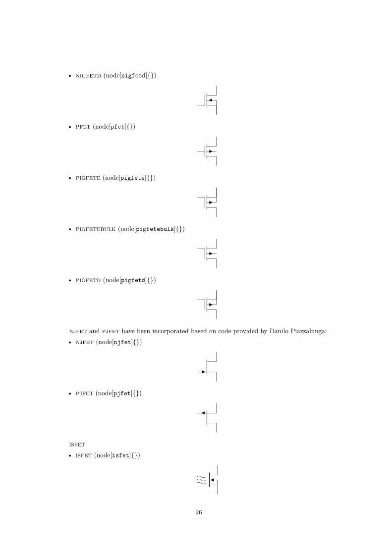
• nigfetd (node[nigfetd])

• pfet (node[pfet])

• pigfete (node[pigfete])

• pigfetebulk (node[pigfetebulk])

• pigfetd (node[pigfetd])

njfet and pjfet have been incorporated based on code provided by Danilo Piazzalunga:• njfet (node[njfet])

• pjfet (node[pjfet])

isfet• isfet (node[isfet])

26

4.3.3 Electronic Tubes

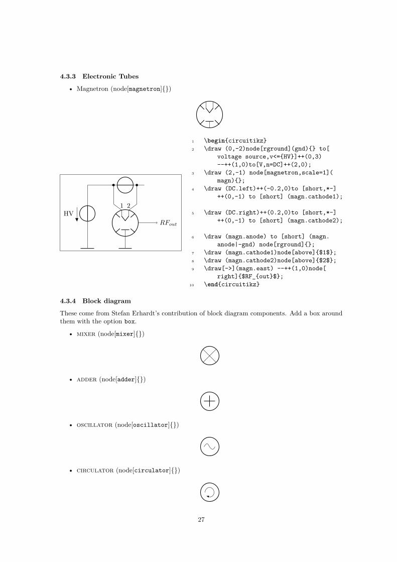
• Magnetron (node[magnetron])

HV1 2

RFout

1 \begincircuitikz2 \draw (0,-2)node[rground](gnd) to[

voltage source,v<=HV]++(0,3)--++(1,0)to[V,n=DC]++(2,0);

3 \draw (2,-1) node[magnetron,scale=1](magn);

4 \draw (DC.left)++(-0.2,0)to [short,*-]++(0,-1) to [short] (magn.cathode1);

5 \draw (DC.right)++(0.2,0)to [short,*-]++(0,-1) to [short] (magn.cathode2);

6 \draw (magn.anode) to [short] (magn.anode|-gnd) node[rground];

7 \draw (magn.cathode1)node[above]$1$;8 \draw (magn.cathode2)node[above]$2$;9 \draw[->](magn.east) --++(1,0)node[

right]$RF_out$;10 \endcircuitikz

4.3.4 Block diagram

These come from Stefan Erhardt’s contribution of block diagram components. Add a box aroundthem with the option box.

• mixer (node[mixer])

• adder (node[adder])

• oscillator (node[oscillator])

• circulator (node[circulator])

27

• wilkinson divider (node[wilkinson])

4.3.5 Switch

• spdt (node[spdt])

• Toggle switch (toggle switch)

4.3.6 Electro-Mechanical Devices

• Motor (node[elmech]M)

M

• Generator (node[elmech]G)

G

Mω

1\begincircuitikz2\draw (2,0) node[elmech](motor)M;3\draw (motor.north) |-(0,2) to [R] ++(0,-2) to[

dcvsource]++(0,-2) -| (motor.bottom);4\draw[thick,->>](motor.right)--++(1,0)node[midway,

above]$\omega$;5\endcircuitikz

ω

1\begincircuitikz2\draw (2,0) node[elmech](motor);3\draw (motor.north) |-(0,2) to [R] ++(0,-2) to[

dcvsource]++(0,-2) -| (motor.bottom);4\draw[thick,->>](motor.center)--++(1.5,0)node[midway,

above]$\omega$;5\endcircuitikz

28

The symbols can also be used along a path, using the transistor-path-syntax(T in front of theshape name, see section 6.6). Don´t forget to use parameter n to name the node and get acces tothe anchors:

M

M

Gω

1\begincircuitikz2\draw (0,0) to [Telmech=M,n=motor] ++(0,-3) to [

Telmech=M] ++(3,0) to [Telmech=G,n=generator]++(0,3) to [R] (0,0);

3\draw[thick,->>](motor.left)--(generator.left)node[midway,above]$\omega$;

4\endcircuitikz

4.4 Double bipolesTransformers automatically use the inductor shape currently selected. These are the three possi-bilities:

• Transformer (cute inductor) (node[transformer])

• Transformer (american inductor) (node[transformer])

• Transformer (european inductor) (node[transformer])

Transformers with core are also available:

• Transformer core (cute inductor) (node[transformer core])

29

• Transformer core (american inductor) (node[transformer core])

• Transformer core (european inductor) (node[transformer core])

• Gyrator (node[gyrator])

• Coupler (node[coupler])

• Coupler, 2 (node[coupler2])

4.5 Logic gates4.5.1 American Logic gates

• American and port (node[american and port])

• American or port (node[american or port])

30

• American not port (node[american not port])

• American nand port (node[american nand port])

• American nor port (node[american nor port])

• American xor port (node[american xor port])

• American xnor port (node[american xnor port])

4.5.2 European Logic gates

• European and port (node[european and port])

&

• European or port (node[european or port])

≥ 1

• European not port (node[european not port])

1

31

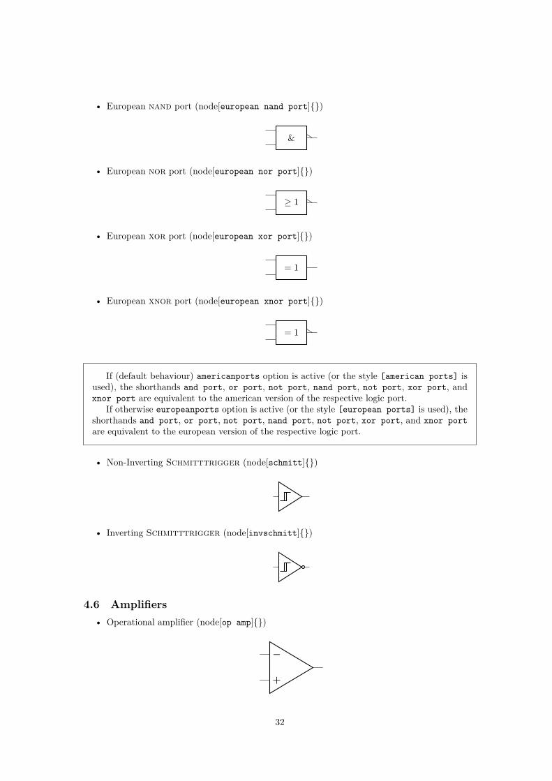
• European nand port (node[european nand port])

&

• European nor port (node[european nor port])

≥ 1

• European xor port (node[european xor port])

= 1

• European xnor port (node[european xnor port])

= 1

If (default behaviour) americanports option is active (or the style [american ports] isused), the shorthands and port, or port, not port, nand port, not port, xor port, andxnor port are equivalent to the american version of the respective logic port.

If otherwise europeanports option is active (or the style [european ports] is used), theshorthands and port, or port, not port, nand port, not port, xor port, and xnor portare equivalent to the european version of the respective logic port.

• Non-Inverting Schmitttrigger (node[schmitt])

• Inverting Schmitttrigger (node[invschmitt])

4.6 Amplifiers• Operational amplifier (node[op amp])

−

+

32

• Operational amplifier compliant to DIN/EN 60617 standard (node[en amp])

−

+

▷ ∞

• Fully differential operational amplifier6 (node[fd op amp])

−

+−+

• transconductance amplifier (node[gm amp])

−

+

• Plain amplifier (node[plain amp])

• Buffer (node[buffer])

4.7 Support shapes• Arrows (current and voltage) (node[currarrow])

• Arrow to draw at its tip, useful for block diagrams. (node[inputarrow])

• Connected terminal (node[circ])6Contributed by Kristofer M. Monisit.

33

• Unconnected terminal (node[ocirc])

• Diamond-style terminal (node[diamondpole])

5 Usage

R11\begincircuitikz2 \draw (0,0) to[R, l=$R_1$] (2,0);3\endcircuitikz

R11\begincircuitikz2 \draw (0,0) to[R=$R_1$] (2,0);3\endcircuitikz

i11\begincircuitikz2 \draw (0,0) to[R, i=$i_1$] (2,0);3\endcircuitikz

v1

1\begincircuitikz2 \draw (0,0) to[R, v=$v_1$] (2,0);3\endcircuitikz

R1

v1

i11\begincircuitikz2 \draw (0,0) to[R=$R_1$, i=$i_1$, v=$v_1$] (2,0);3\endcircuitikz

R1

v1

i11\begincircuitikz2 \draw (0,0) to[R=$R_1$, i=$i_1$, v=$v_1$] (2,0);3\endcircuitikz

Long names/styles for the bipoles can be used:

1 kΩ 1\begincircuitikz\draw2 (0,0) to[resistor=1<\kilo\ohm>] (2,0)3;\endcircuitikz

5.1 Labels and AnnotationsSince Version 0.7, beside the original label (l) option, there is a new option to place a second label,called annotation (a) at each bipole. Up to now this is a beta-test and there can be problems. Forexample, up to now this option is not compatible with the concurrent use of voltage labels.

The position of (a) and (l) labels can be adjusted with _ and , respectively.

R1

1 kΩ

1\begincircuitikz2 \draw (0,0) to[R, l=$R_1$,a=1<\kilo\ohm>] (2,0);3\endcircuitikz

34

R1

1 kΩ 1\begincircuitikz2 \draw (0,0) to[R, l_=$R_1$,a^=1<\kilo\ohm>] (2,0);3\endcircuitikz

The default orientation of labels is controlled by the options smartlabels, rotatelabels andstraightlabels (or the corresponding label/align keys). Here are examples to see the differ-ences:

0

4590

135

180

-90

-45

-135

1\begincircuitikz2\ctikzsetlabel/align = straight3\def\DIR0,45,90,135,180,-90,-45,-1354\foreach \i in \DIR 5 \draw (0,0) to[R=\i, *-o] (\i:2.5);67\endcircuitikz

0

4590

135

180

-90

-45

-135

1\begincircuitikz2\ctikzsetlabel/align = rotate3\def\DIR0,45,90,135,180,-90,-45,-1354\foreach \i in \DIR 5 \draw (0,0) to[R=\i, *-o] (\i:2.5);67\endcircuitikz

0

4590135

180

-90

-45

-135

1\begincircuitikz2\ctikzsetlabel/align = smart3\def\DIR0,45,90,135,180,-90,-45,-1354\foreach \i in \DIR 5 \draw (0,0) to[R=\i, *-o] (\i:2.5);67\endcircuitikz

5.2 CurrentsThe counting direction of currents and voltages have changed with version 0.5, for compabilityreasons there is a option to use the olddirections(see options). For the new scheme, the followingrules apply:

35

• Normal bipoles: currents and voltages are counted positiv in drawing direction.

• Current Sources: current is counted positiv in drawing direction, voltage in oppositedirection

• Voltage Sources: voltage is counted positiv in drawing direction, current in oppositedirection

With this convention, the power at loads is positive and negative at sources.

i11\begincircuitikz2 \draw (0,0) to[R, i^>=$i_1$] (2,0);3\endcircuitikz

i1

1\begincircuitikz2 \draw (0,0) to[R, i_>=$i_1$] (2,0);3\endcircuitikz

i11\begincircuitikz2 \draw (0,0) to[R, i^<=$i_1$] (2,0);3\endcircuitikz

i1

1\begincircuitikz2 \draw (0,0) to[R, i_<=$i_1$] (2,0);3\endcircuitikz

i11\begincircuitikz2 \draw (0,0) to[R, i>^=$i_1$] (2,0);3\endcircuitikz

i1

1\begincircuitikz2 \draw (0,0) to[R, i>_=$i_1$] (2,0);3\endcircuitikz

i11\begincircuitikz2 \draw (0,0) to[R, i<^=$i_1$] (2,0);3\endcircuitikz

i1

1\begincircuitikz2 \draw (0,0) to[R, i<_=$i_1$] (2,0);3\endcircuitikz

Also

i11\begincircuitikz2 \draw (0,0) to[R, i<=$i_1$] (2,0);3\endcircuitikz

i11\begincircuitikz2 \draw (0,0) to[R, i>=$i_1$] (2,0);3\endcircuitikz

i11\begincircuitikz2 \draw (0,0) to[R, i^=$i_1$] (2,0);3\endcircuitikz

36

i1

1\begincircuitikz2 \draw (0,0) to[R, i_=$i_1$] (2,0);3\endcircuitikz

10V

i1

1\begincircuitikz2 \draw (0,0) to[V=10V, i_=$i_1$] (2,0);3\endcircuitikz

10V

i1

1\begincircuitikz2 \draw (0,0) to[V<=10V, i_=$i_1$] (2,0);3\endcircuitikz

−+

10V

i1

1\begincircuitikz[american]2 \draw (0,0) to[V=10V, i_=$i_1$] (2,0);3\endcircuitikz

− +

10V

i1

1\begincircuitikz[american]2 \draw (0,0) to[V=10V,invert, i_=$i_1$] (2,0);3\endcircuitikz

1A

i1

1\begincircuitikz[american]2 \draw (0,0) to[dcisource=1A, i_=$i_1$] (2,0);3\endcircuitikz

1A

i1

1\begincircuitikz[american]2 \draw (0,0) to[dcisource=1A,invert, i_=$i_1$] (2,0);3\endcircuitikz

5.3 FlowsAs an alternative for the current arrows, you can also use the following flows. They can also beused to indicate thermal or power flows. The syntax is pretty the same as for currents.

This is a new beta feature since version 0.8.3, therefore, please provide bugreports or hints tooptimize this feature regarding placement and appearance! This means, that the appearance maychange in the future!

i11\begincircuitikz2 \draw (0,0) to[R, f=$i_1$] (3,0);3\endcircuitikz

i11\begincircuitikz2 \draw (0,0) to[R, f<=$i_1$] (3,0);3\endcircuitikz

i1

1\begincircuitikz2 \draw (0,0) to[R, f_=$i_1$] (3,0);3\endcircuitikz

37

i1

1\begincircuitikz2 \draw (0,0) to[R, f_>=$i_1$] (3,0);3\endcircuitikz

i11\begincircuitikz2 \draw (0,0) to[R, f<^=$i_1$] (3,0);3\endcircuitikz

i1

1\begincircuitikz2 \draw (0,0) to[R, f<_=$i_1$] (3,0);3\endcircuitikz

i1

1\begincircuitikz2 \draw (0,0) to[R, f>_=$i_1$] (3,0);3\endcircuitikz

5.4 VoltagesSee introduction note at Currents (chapter 5.2, page 35)!

5.4.1 European style

The default, with arrows. Use option europeanvoltage or style [european voltages].

v1 1\begincircuitikz[european voltages]2 \draw (0,0) to[R, v^>=$v_1$] (2,0);3\endcircuitikz

v1 1\begincircuitikz[european voltages]2 \draw (0,0) to[R, v^<=$v_1$] (2,0);3\endcircuitikz

v1

1\begincircuitikz[european voltages]2 \draw (0,0) to[R, v_>=$v_1$] (2,0);3\endcircuitikz

v1

1\begincircuitikz[european voltages]2 \draw (0,0) to[R, v_<=$v_1$] (2,0);3\endcircuitikz

10V

i1

1\begincircuitikz2 \draw (0,0) to[V=10V, i_=$i_1$] (2,0);3\endcircuitikz

10V

i1

1\begincircuitikz2 \draw (0,0) to[V<=10V, i_=$i_1$] (2,0);3\endcircuitikz

u1

1A 1\begincircuitikz2 \draw (0,0) to[I=1A, v_=$u_1$] (2,0);3\endcircuitikz

38

u1

1A 1\begincircuitikz2 \draw (0,0) to[I<=1A, v_=$u_1$] (2,0);3\endcircuitikz

1A

u1

1\begincircuitikz2 \draw (0,0) to[I=$~$,l=1A, v_=$u_1$] (2,0);3\endcircuitikz

1A

u1

1\begincircuitikz2 \draw (0,0) to[I,l=1A, v_=$u_1$] (2,0);3\endcircuitikz

5.4.2 American style

For those who like it (not me). Use option americanvoltage or set [american voltages].

+ −v11\begincircuitikz[american voltages]2 \draw (0,0) to[R, v^>=$v_1$] (2,0);3\endcircuitikz

− +v1

1\begincircuitikz[american voltages]2 \draw (0,0) to[R, v^<=$v_1$] (2,0);3\endcircuitikz

+ −v1

1\begincircuitikz[american voltages]2 \draw (0,0) to[R, v_>=$v_1$] (2,0);3\endcircuitikz

− +v1

1\begincircuitikz[american voltages]2 \draw (0,0) to[R, v_<=$v_1$] (2,0);3\endcircuitikz

− +u1

1A 1\begincircuitikz[american]2 \draw (0,0) to[I=1A, v_=$u_1$] (2,0);3\endcircuitikz

+ −i1

1A 1\begincircuitikz[american]2 \draw (0,0) to[I<=1A, v_=$i_1$] (2,0);3\endcircuitikz

5.5 Nodes1\begincircuitikz2 \draw (0,0) to[R, o-o] (2,0);3\endcircuitikz

1\begincircuitikz2 \draw (0,0) to[R, -o] (2,0);3\endcircuitikz

39

1\begincircuitikz2 \draw (0,0) to[R, o-] (2,0);3\endcircuitikz

1\begincircuitikz2 \draw (0,0) to[R, *-*] (2,0);3\endcircuitikz

1\begincircuitikz2 \draw (0,0) to[R, -*] (2,0);3\endcircuitikz

1\begincircuitikz2 \draw (0,0) to[R, *-] (2,0);3\endcircuitikz

1\begincircuitikz2 \draw (0,0) to[R, d-d] (2,0);3\endcircuitikz

1\begincircuitikz2 \draw (0,0) to[R, -d] (2,0);3\endcircuitikz

1\begincircuitikz2 \draw (0,0) to[R, d-] (2,0);3\endcircuitikz

1\begincircuitikz2 \draw (0,0) to[R, o-*] (2,0);3\endcircuitikz

1\begincircuitikz2 \draw (0,0) to[R, *-o] (2,0);3\endcircuitikz

1\begincircuitikz2 \draw (0,0) to[R, o-d] (2,0);3\endcircuitikz

1\begincircuitikz2 \draw (0,0) to[R, d-o] (2,0);3\endcircuitikz

1\begincircuitikz2 \draw (0,0) to[R, *-d] (2,0);3\endcircuitikz

1\begincircuitikz2 \draw (0,0) to[R, d-*] (2,0);3\endcircuitikz

40

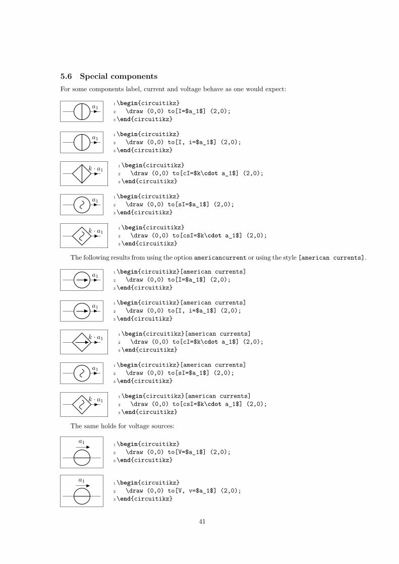
5.6 Special componentsFor some components label, current and voltage behave as one would expect:

a11\begincircuitikz2 \draw (0,0) to[I=$a_1$] (2,0);3\endcircuitikz

a11\begincircuitikz2 \draw (0,0) to[I, i=$a_1$] (2,0);3\endcircuitikz

k · a1 1\begincircuitikz2 \draw (0,0) to[cI=$k\cdot a_1$] (2,0);3\endcircuitikz

a11\begincircuitikz2 \draw (0,0) to[sI=$a_1$] (2,0);3\endcircuitikz

k · a1 1\begincircuitikz2 \draw (0,0) to[csI=$k\cdot a_1$] (2,0);3\endcircuitikz

The following results from using the option americancurrent or using the style [american currents].

a11\begincircuitikz[american currents]2 \draw (0,0) to[I=$a_1$] (2,0);3\endcircuitikz

a11\begincircuitikz[american currents]2 \draw (0,0) to[I, i=$a_1$] (2,0);3\endcircuitikz

k · a1 1\begincircuitikz[american currents]2 \draw (0,0) to[cI=$k\cdot a_1$] (2,0);3\endcircuitikz

a11\begincircuitikz[american currents]2 \draw (0,0) to[sI=$a_1$] (2,0);3\endcircuitikz

k · a1 1\begincircuitikz[american currents]2 \draw (0,0) to[csI=$k\cdot a_1$] (2,0);3\endcircuitikz

The same holds for voltage sources:

a1 1\begincircuitikz2 \draw (0,0) to[V=$a_1$] (2,0);3\endcircuitikz

a1 1\begincircuitikz2 \draw (0,0) to[V, v=$a_1$] (2,0);3\endcircuitikz

41

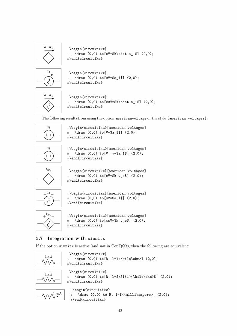
k · a11\begincircuitikz2 \draw (0,0) to[cV=$k\cdot a_1$] (2,0);3\endcircuitikz

a1 1\begincircuitikz2 \draw (0,0) to[sV=$a_1$] (2,0);3\endcircuitikz

k · a11\begincircuitikz2 \draw (0,0) to[csV=$k\cdot a_1$] (2,0);3\endcircuitikz

The following results from using the option americanvoltage or the style [american voltages].

−+

a1 1\begincircuitikz[american voltages]2 \draw (0,0) to[V=$a_1$] (2,0);3\endcircuitikz

−+

a1 1\begincircuitikz[american voltages]2 \draw (0,0) to[V, v=$a_1$] (2,0);3\endcircuitikz

−+

kve 1\begincircuitikz[american voltages]2 \draw (0,0) to[cV=$k v_e$] (2,0);3\endcircuitikz

+ −a1 1\begincircuitikz[american voltages]2 \draw (0,0) to[sV=$a_1$] (2,0);3\endcircuitikz

+ −kve 1\begincircuitikz[american voltages]2 \draw (0,0) to[csV=$k v_e$] (2,0);3\endcircuitikz

5.7 Integration with siunitxIf the option siunitx is active (and not in ConTEXt), then the following are equivalent:

1 kΩ 1\begincircuitikz2 \draw (0,0) to[R, l=1<\kilo\ohm>] (2,0);3\endcircuitikz

1 kΩ 1\begincircuitikz2 \draw (0,0) to[R, l=$\SI1\kilo\ohm$] (2,0);3\endcircuitikz

1mA1\begincircuitikz2 \draw (0,0) to[R, i=1<\milli\ampere>] (2,0);3\endcircuitikz

42

1mA1\begincircuitikz2 \draw (0,0) to[R, i=$\SI1\milli\ampere$] (2,0);3\endcircuitikz

1V

1\begincircuitikz2 \draw (0,0) to[R, v=1<\volt>] (2,0);3\endcircuitikz

1V

1\begincircuitikz2 \draw (0,0) to[R, v=$\SI1\volt$] (2,0);3\endcircuitikz

5.8 Mirroring and InvertingBipole paths can also mirrored and inverted (or reverted) to change the drawing direction.

1\begincircuitikz2 \draw (0,0) to[pD] (2,0);3\endcircuitikz

1\begincircuitikz2 \draw (0,0) to[pD, mirror] (2,0);3\endcircuitikz

1\begincircuitikz2 \draw (0,0) to[pD, invert] (2,0);3\endcircuitikz

Placing labels, currents and voltages works also, please note, that mirroring and inverting doesnot incfluence the positioning of labels and voltages. Labels are by default above/right of thebipole and voltages below/left, respectively.

T

v

i11\begincircuitikz2 \draw (0,0) to[ospst=T, i=$i_1$, v=$v$] (2,0);3\endcircuitikz

T

v

i11\begincircuitikz2 \draw (0,0) to[ospst=T, mirror, i=$i_1$, v=$v$] (2,0);3\endcircuitikz

T

v

i11\begincircuitikz2 \draw (0,0) to[ospst=T, invert, i=$i_1$, v=$v$] (2,0);3\endcircuitikz

T

v

i11\begincircuitikz2 \draw (0,0) to[ospst=T,mirror,invert, i=$i_1$, v=$v$] (2,0);3\endcircuitikz

5.9 Putting them together

1 kΩ

1mA

1\begincircuitikz2 \draw (0,0) to[R=1<\kilo\ohm>,3 i>_=1<\milli\ampere>, o-*] (3,0);4\endcircuitikz

43

vD

1mA 1\begincircuitikz2 \draw (0,0) to[D*, v=$v_D$,3 i=1<\milli\ampere>, o-*] (3,0);4\endcircuitikz

5.10 Line joins between Path ComponentsLine joins should be calculated correctly, if the were on the same path and if the path is not closed.For example, the following path is not closed correctly(–cycle does not work here!):

1 \begintikzpicture[line width=3pt,european]2 \draw (0,0) to[R]++(2,0)to[R]++(0,2)3 --++(-2,0)to[R]++(0,-2);4 \draw[red,line width=1pt] circle(2mm);5 \endtikzpicture

To correct the line ending, there are support shapes to fill the missing rectangle. They can beused like the support shapes(*,o,d) using a dot (.) on one or both ends of a component(have alook at the last resistor in this example:

1 \begintikzpicture[line width=3pt,european]2 \draw (0,0) to[R]++(2,0)to[R]++(0,2)3 --++(-2,0)to[R,-.]++(0,-2);4 \draw[red,line width=1pt] circle(2mm);5 \endtikzpicture

6 Not only bipolesSince only bipoles (but see section 6.6) can be placed ”along a line”, components with more thantwo terminals are placed as nodes:

+5V

-5V

1\begincircuitikz2\draw (0,0) node[npn](npn) at (0,0) ;3\draw (npn.C) --++(0,0.5) node[vcc]+5\,\textnormalV;4\draw (npn.E) --++(0,-0.5) node[vee]-5\,\textnormalV;5\endcircuitikz

6.1 AnchorsIn order to allow connections with other components, all components define anchors.

6.1.1 Logical ports

All logical ports, except not, have two inputs and one output. They are called respectively in 1,in 2, out:

44

12

3

1\begincircuitikz \draw2 (0,0) node[and port] (myand) 3 (myand.in 1) node[anchor=east] 14 (myand.in 2) node[anchor=east] 25 (myand.out) node[anchor=west] 36;\endcircuitikz

1\begincircuitikz \draw2 (0,2) node[and port] (myand1) 3 (0,0) node[and port] (myand2) 4 (2,1) node[xnor port] (myxnor) 5 (myand1.out) -| (myxnor.in 1)6 (myand2.out) -| (myxnor.in 2)7;\endcircuitikz

In the case of not, there are only in and out (although for compatibility reasons in 1 is stilldefined and equal to in):

1\begincircuitikz \draw2 (1,0) node[not port] (not1) 3 (3,0) node[not port] (not2) 4 (0,0) -- (not1.in)5 (not2.in) -- (not1.out)6 ++(0,-1) node[ground] to[C] (not1.out)7 (not2.out) -| (4,1) -| (0,0)8;\endcircuitikz

6.1.2 Transistors

For nmos, pmos, nfet, nigfete, nigfetd, pfet, pigfete, and pigfetd transistors one hasbase, gate, source and drain anchors (which can be abbreviated with B, G, S and D):

G

D

S

1\begincircuitikz \draw2 (0,0) node[nmos] (mos) 3 (mos.gate) node[anchor=east] G4 (mos.drain) node[anchor=south] D5 (mos.source) node[anchor=north] S6;\endcircuitikz

G

D

S

Bulk

1\begincircuitikz \draw2 (0,0) node[pigfete] (pigfete) 3 (pigfete.G) node[anchor=east] G4 (pigfete.D) node[anchor=north] D5 (pigfete.S) node[anchor=south] S6 (pigfete.bulk) node[anchor=west] Bulk7;\endcircuitikz

Similarly njfet and pjfet have gate, source and drain anchors (which can be abbreviatedwith G, S and D):

G

D

S 1\begincircuitikz \draw2 (0,0) node[pjfet] (pjfet) 3 (pjfet.G) node[anchor=east] G4 (pjfet.D) node[anchor=north] D5 (pjfet.S) node[anchor=south] S6;\endcircuitikz

45

For npn, pnp, nigbt, and pigbt transistors the anchors are base, emitter and collectoranchors (which can be abbreviated with B, E and C):

B

C

E

1\begincircuitikz \draw2 (0,0) node[npn] (npn) 3 (npn.base) node[anchor=east] B4 (npn.collector) node[anchor=south] C5 (npn.emitter) node[anchor=north] E6;\endcircuitikz

B

C

E 1\begincircuitikz \draw2 (0,0) node[pigbt] (pigbt) 3 (pigbt.B) node[anchor=east] B4 (pigbt.C) node[anchor=north] C5 (pigbt.E) node[anchor=south] E6;\endcircuitikz

Here is one composite example (please notice that the xscale=-1 style would also reflect thelabel of the transistors, so here a new node is added and its text is used, instead of that of pnp1):

2

1

1\begincircuitikz \draw2 (0,0) node[pnp] (pnp2) 23 (pnp2.B) node[pnp, xscale=-1, anchor=B] (pnp1) 4 (pnp1) node 15 (pnp1.C) node[npn, anchor=C] (npn1) 6 (pnp2.C) node[npn, xscale=-1, anchor=C] (npn2) 7 (pnp1.E) -- (pnp2.E) (npn1.E) -- (npn2.E)8 (pnp1.B) node[circ] |- (pnp2.C) node[circ] 9;\endcircuitikz

Similarly, transistors and other components can be reflected vertically:

BulkG

D

S

1\begincircuitikz \draw2 (0,0) node[pigfete, yscale=-1] (pigfete) 3 (pigfete.bulk) node[anchor=west] Bulk4 (pigfete.G) node[anchor=east] G5 (pigfete.D) node[anchor=south] D6 (pigfete.S) node[anchor=north] S7;\endcircuitikz

R1

1 \begincircuitikz2 \draw (0,2)3 node[rground, yscale=-1] 4 to[R=$R_1$] (0,0)5 node[sground] ;6 \endcircuitikz

6.1.3 Other tripoles

When inserting a thrystor, a triac or a potentiometer, one needs to refer to the third node–gate(gate or G) for the former two; wiper (wiper or W) for the latter one. This is done by giving aname to the bipole:

46

1\begincircuitikz \draw2 (0,0) to[Tr, n=TRI] (2,0)3 to[pR, n=POT] (4,0);4 \draw[dashed] (TRI.G) -| (POT.wiper)5;\endcircuitikz

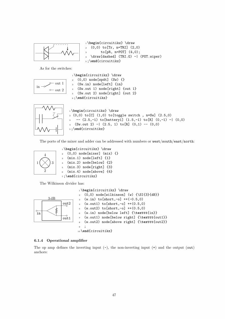
As for the switches:

inout 1

out 2

1\begincircuitikz \draw2 (0,0) node[spdt] (Sw) 3 (Sw.in) node[left] in4 (Sw.out 1) node[right] out 15 (Sw.out 2) node[right] out 26;\endcircuitikz

1\begincircuitikz \draw2 (0,0) to[C] (1,0) to[toggle switch , n=Sw] (2.5,0)3 -- (2.5,-1) to[battery1] (1.5,-1) to[R] (0,-1) -| (0,0)4 (Sw.out 2) -| (2.5, 1) to[R] (0,1) -- (0,0)5;\endcircuitikz

The ports of the mixer and adder can be addressed with numbers or west/south/east/north:

1

2

3

41\begincircuitikz \draw2 (0,0) node[mixer] (mix) 3 (mix.1) node[left] 14 (mix.2) node[below] 25 (mix.3) node[right] 36 (mix.4) node[above] 47;\endcircuitikz

The Wilkinson divider has:

3 dB

inout1

out2

1\begincircuitikz \draw2 (0,0) node[wilkinson] (w) \SI3dB3 (w.in) to[short,-o] ++(-0.5,0)4 (w.out1) to[short,-o] ++(0.5,0)5 (w.out2) to[short,-o] ++(0.5,0)6 (w.in) node[below left] \textttin7 (w.out1) node[below right] \textttout18 (w.out2) node[above right] \textttout29 ;

10\endcircuitikz

6.1.4 Operational amplifier

The op amp defines the inverting input (-), the non-inverting input (+) and the output (out)anchors:

47

−

+v+

v−

vo

5V

-5V

1\begincircuitikz \draw2 (0,0) node[op amp] (opamp) 3 (opamp.+) node[left] $v_+$4 (opamp.-) node[left] $v_-$5 (opamp.out) node[right] $v_o$6 (opamp.up) --++(0,0.5) node[vcc]5\,\textnormalV7 (opamp.down) --++(0,-0.5) node[vee]-5\,\textnormalV

8;\endcircuitikz

There are also two more anchors defined, up and down, for the power supplies:

−

+v+

v−

vo

12V

1\begincircuitikz \draw2 (0,0) node[op amp] (opamp) 3 (opamp.+) node[left] $v_+$4 (opamp.-) node[left] $v_-$5 (opamp.out) node[right] $v_o$6 (opamp.down) node[ground] 7 (opamp.up) ++ (0,.5) node[above] \SI12\volt8 -- (opamp.up)9;\endcircuitikz

The fully differential op amp defines two outputs:

−

+−+

v+

v− out +

out -

1\begincircuitikz \draw2 (0,0) node[fd op amp] (opamp) 3 (opamp.+) node[left] $v_+$4 (opamp.-) node[left] $v_-$5 (opamp.out +) node[right] out +6 (opamp.out -) node[right] out -7 (opamp.down) node[ground] 8;\endcircuitikz

6.1.5 Double bipoles

All the (few, actually) double bipoles/quadrupoles have the four anchors, two for each port. Thefirst port, to the left, is port A, having the anchors A1 (up) and A2 (down); same for port B. Theyalso expose the base anchor, for labelling:

A1

A2

B1

B2

K1\begincircuitikz \draw2 (0,0) node[transformer] (T) 3 (T.A1) node[anchor=east] A14 (T.A2) node[anchor=east] A25 (T.B1) node[anchor=west] B16 (T.B2) node[anchor=west] B27 (T.base) nodeK8;\endcircuitikz

A1

A2

B1

B2

K1\begincircuitikz \draw2 (0,0) node[gyrator] (G) 3 (G.A1) node[anchor=east] A14 (G.A2) node[anchor=east] A25 (G.B1) node[anchor=west] B16 (G.B2) node[anchor=west] B27 (G.base) nodeK8;\endcircuitikz

48

However:

10 dB

1 2

34

1\begincircuitikz \draw2 (0,0) node[coupler] (c) \SI10dB3 (c.1) to[short,-o] ++(-0.5,0)4 (c.2) to[short,-o] ++(0.5,0)5 (c.3) to[short,-o] ++(0.5,0)6 (c.4) to[short,-o] ++(-0.5,0)7 (c.1) node[below left] \texttt18 (c.2) node[below right] \texttt29 (c.3) node[above right] \texttt3

10 (c.4) node[above left] \texttt411 ;12\endcircuitikz

3 dB

1 2

34

1\begincircuitikz \draw2 (0,0) node[coupler2] (c) \SI3dB3 (c.1) to[short,-o] ++(-0.5,0)4 (c.2) to[short,-o] ++(0.5,0)5 (c.3) to[short,-o] ++(0.5,0)6 (c.4) to[short,-o] ++(-0.5,0)7 (c.1) node[below left] \texttt18 (c.2) node[below right] \texttt29 (c.3) node[above right] \texttt3

10 (c.4) node[above left] \texttt411 ;12\endcircuitikz

6.2 Input arrowsTwo ports

With the option > you can draw an arrow to the input of the block diagram symbols.

AD

1\begincircuitikz \draw2 (0,0) to[short,o-] ++(0.3,0)3 to[lowpass,>] ++(2,0)4 to[adc,>] ++(2,0)5 to[short,-o] ++(0.3,0);6\endcircuitikz

Multi ports

Since inputs and outputs can vary, input arrows can be placed as nodes. Note that you have torotate the arrow on your own:

1\begincircuitikz \draw2 (0,0) node[mixer] (m) 3 (m.1) to[short,-o] ++(-1,0)4 (m.2) to[short,-o] ++(0,-1)5 (m.3) to[short,-o] ++(1,0)6 (m.1) node[inputarrow] 7 (m.2) node[inputarrow,rotate=90] ;8\endcircuitikz

49

6.3 Labels and custom twoport boxesSome twoports have the option to place a normal label (l=) and a inner label (t=).

LNA

F=0.9dB

1\begincircuitikz2 \ctikzsetbipoles/amp/width=0.93 \draw (0,0) to[amp,t=LNA,l_=$F=0.9\,$dB,o-o] ++(3,0);4\endcircuitikz

6.4 Box optionSome devices have the possibility to add a box around them. The inner symbol scales down to fitinside the box.

1\begincircuitikz \draw2 (0,0) node[mixer,box,anchor=east] (m) 3 to[amp,box,>,-o] ++(2.5,0)4 (m.west) node[inputarrow] to[short,-o]

++(-0.8,0)5 (m.south) node[inputarrow,rotate=90] --6 ++(0,-0.7) node[oscillator,box,anchor=north] ;7\endcircuitikz

6.5 Dash optional partsTo show that a device is optional, you can dash it. The inner symbol will be kept with solid lines.

10 dB opt.1\begincircuitikz2 \draw (0,0) to[amp,l=\SI10dB] ++(2.5,0);3 \draw[dashed] (2.5,0) to[lowpass,l=opt.]

++(2.5,0);4\endcircuitikz

6.6 Transistor pathsFor syntactical convenience transistors can be placed using the normal path notation used forbipoles. The transitor type can be specified by simply adding a “T” (for transistor) in front of thenode name of the transistor. It will be placed with the base/gate orthogonal to the direction ofthe path:

1

2 3 1\begincircuitikz \draw2 (0,0) node[njfet] 13 (-1,2) to[Tnjfet=2] (1,2)4 to[Tnjfet=3, mirror] (3,2);5;\endcircuitikz

Access to the gate and/or base nodes can be gained by naming the transistors with the n orname path style:

50

1\begincircuitikz \draw[yscale=1.1, xscale=.8]2 (2,4.5) -- (0,4.5) to[Tpmos, n=p1] (0,3)3 to[Tnmos, n=n1] (0,1.5)4 to[Tnmos, n=n2] (0,0) node[ground] 5 (2,4.5) to[Tpmos,n=p2] (2,3) to[short, -*] (0,3)6 (p1.G) -- (n1.G) to[short, *-o] ($(n1.G)+(3,0)$)7 (n2.G) ++(2,0) node[circ] -| (p2.G)8 (n2.G) to[short, -o] ($(n2.G)+(3,0)$)9 (0,3) to[short, -o] (-1,3)

10;\endcircuitikz

The name property is available also for bipoles, although this is useful mostly for triac, poten-tiometer and thyristor (see 4.2.5).

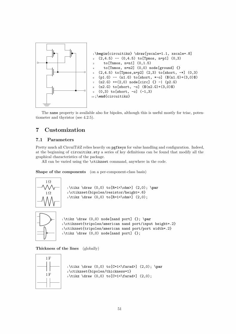
7 Customization7.1 ParametersPretty much all CircuiTikZ relies heavily on pgfkeys for value handling and configuration. Indeed,at the beginning of circuitikz.sty a series of key definitions can be found that modify all thegraphical characteristics of the package.

All can be varied using the \ctikzset command, anywhere in the code.

Shape of the components (on a per-component-class basis)

1Ω

1Ω1\tikz \draw (0,0) to[R=1<\ohm>] (2,0); \par2\ctikzsetbipoles/resistor/height=.63\tikz \draw (0,0) to[R=1<\ohm>] (2,0);

1\tikz \draw (0,0) node[nand port] ; \par2\ctikzsettripoles/american nand port/input height=.23\ctikzsettripoles/american nand port/port width=.24\tikz \draw (0,0) node[nand port] ;

Thickness of the lines (globally)

1F

1F

1\tikz \draw (0,0) to[C=1<\farad>] (2,0); \par2\ctikzsetbipoles/thickness=13\tikz \draw (0,0) to[C=1<\farad>] (2,0);

51

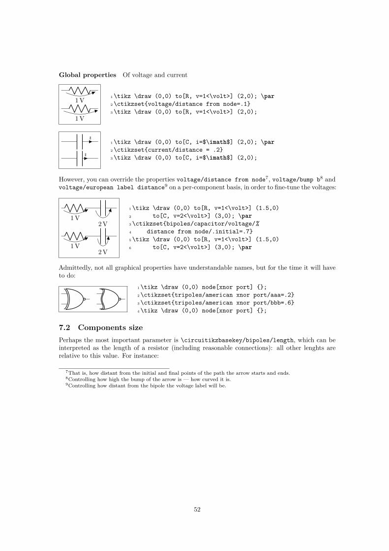
Global properties Of voltage and current

1V

1V

1\tikz \draw (0,0) to[R, v=1<\volt>] (2,0); \par2\ctikzsetvoltage/distance from node=.13\tikz \draw (0,0) to[R, v=1<\volt>] (2,0);

ı

ı

1\tikz \draw (0,0) to[C, i=$\imath$] (2,0); \par2\ctikzsetcurrent/distance = .23\tikz \draw (0,0) to[C, i=$\imath$] (2,0);

However, you can override the properties voltage/distance from node7, voltage/bump b8 andvoltage/european label distance9 on a per-component basis, in order to fine-tune the voltages:

1V2V

1V2V

1\tikz \draw (0,0) to[R, v=1<\volt>] (1.5,0)2 to[C, v=2<\volt>] (3,0); \par3\ctikzsetbipoles/capacitor/voltage/%4 distance from node/.initial=.75\tikz \draw (0,0) to[R, v=1<\volt>] (1.5,0)6 to[C, v=2<\volt>] (3,0); \par

Admittedly, not all graphical properties have understandable names, but for the time it will haveto do:

1\tikz \draw (0,0) node[xnor port] ;2\ctikzsettripoles/american xnor port/aaa=.23\ctikzsettripoles/american xnor port/bbb=.64\tikz \draw (0,0) node[xnor port] ;

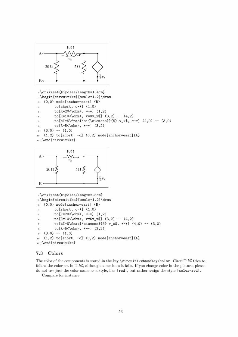
7.2 Components sizePerhaps the most important parameter is \circuitikzbasekey/bipoles/length, which can beinterpreted as the length of a resistor (including reasonable connections): all other lenghts arerelative to this value. For instance:

7That is, how distant from the initial and final points of the path the arrow starts and ends.8Controlling how high the bump of the arrow is — how curved it is.9Controlling how distant from the bipole the voltage label will be.

52

B

20Ω

10Ω

vx

S5vx

5Ω

A

1\ctikzsetbipoles/length=1.4cm2\begincircuitikz[scale=1.2]\draw3 (0,0) node[anchor=east] B4 to[short, o-*] (1,0)5 to[R=20<\ohm>, *-*] (1,2)6 to[R=10<\ohm>, v=$v_x$] (3,2) -- (4,2)7 to[cI=$\frac\si\siemens5 v_x$, *-*] (4,0) -- (3,0)8 to[R=5<\ohm>, *-*] (3,2)9 (3,0) -- (1,0)

10 (1,2) to[short, -o] (0,2) node[anchor=east]A11;\endcircuitikz

B

20Ω

10Ω

vx

S5vx

5Ω

A

1\ctikzsetbipoles/length=.8cm2\begincircuitikz[scale=1.2]\draw3 (0,0) node[anchor=east] B4 to[short, o-*] (1,0)5 to[R=20<\ohm>, *-*] (1,2)6 to[R=10<\ohm>, v=$v_x$] (3,2) -- (4,2)7 to[cI=$\frac\siemens5 v_x$, *-*] (4,0) -- (3,0)8 to[R=5<\ohm>, *-*] (3,2)9 (3,0) -- (1,0)

10 (1,2) to[short, -o] (0,2) node[anchor=east]A11;\endcircuitikz

7.3 ColorsThe color of the components is stored in the key \circuitikzbasekey/color. CircuiTikZ tries tofollow the color set in TikZ, although sometimes it fails. If you change color in the picture, pleasedo not use just the color name as a style, like [red], but rather assign the style [color=red].

Compare for instance

53

1\begincircuitikz \draw[red]2 (0,2) node[and port] (myand1) 3 (0,0) node[and port] (myand2) 4 (2,1) node[xnor port] (myxnor) 5 (myand1.out) -| (myxnor.in 1)6 (myand2.out) -| (myxnor.in 2)7;\endcircuitikz

and

1\begincircuitikz \draw[color=red]2 (0,2) node[and port] (myand1) 3 (0,0) node[and port] (myand2) 4 (2,1) node[xnor port] (myxnor) 5 (myand1.out) -| (myxnor.in 1)6 (myand2.out) -| (myxnor.in 2)7;\endcircuitikz

One can of course change the color in medias res:

1\begincircuitikz \draw2 (0,0) node[pnp, color=blue] (pnp2) 3 (pnp2.B) node[pnp, xscale=-1, anchor=B, color=brown] (pnp1) 4 (pnp1.C) node[npn, anchor=C, color=green] (npn1) 5 (pnp2.C) node[npn, xscale=-1, anchor=C, color=magenta] (npn2) 6 (pnp1.E) -- (pnp2.E) (npn1.E) -- (npn2.E)7 (pnp1.B) node[circ] |- (pnp2.C) node[circ] 8;\endcircuitikz

The all-in-one stream of bipoles poses some challanges, as only the actual body of the bipole,and not the connecting lines, will be rendered in the specified color. Also, please notice the curlybraces around the to:

1V

1Ω

1F

1\begincircuitikz \draw2 (0,0) to[V=1<\volt>] (0,2)3 to[R=1<\ohm>, color=red] (2,2) 4 to[C=1<\farad>] (2,0) -- (0,0)5;\endcircuitikz

Which, for some bipoles, can be frustrating:

54

1V

1Ω

1F

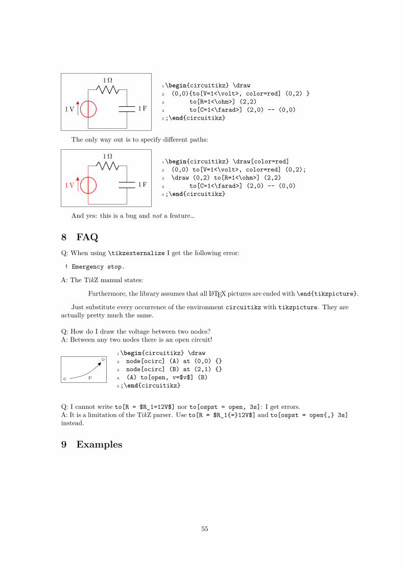
1\begincircuitikz \draw2 (0,0)to[V=1<\volt>, color=red] (0,2) 3 to[R=1<\ohm>] (2,2)4 to[C=1<\farad>] (2,0) -- (0,0)5;\endcircuitikz

The only way out is to specify different paths:

1V

1Ω

1F

1\begincircuitikz \draw[color=red]2 (0,0) to[V=1<\volt>, color=red] (0,2);3 \draw (0,2) to[R=1<\ohm>] (2,2)4 to[C=1<\farad>] (2,0) -- (0,0)5;\endcircuitikz

And yes: this is a bug and not a feature…

8 FAQQ: When using \tikzexternalize I get the following error:

! Emergency stop.

A: The TikZ manual states:

Furthermore, the library assumes that all LATEX pictures are ended with \endtikzpicture.

Just substitute every occurrence of the environment circuitikz with tikzpicture. They areactually pretty much the same.

Q: How do I draw the voltage between two nodes?A: Between any two nodes there is an open circuit!

v

1\begincircuitikz \draw2 node[ocirc] (A) at (0,0) 3 node[ocirc] (B) at (2,1) 4 (A) to[open, v=$v$] (B)5;\endcircuitikz

Q: I cannot write to[R = $R_1=12V$] nor to[ospst = open, 3s]: I get errors.A: It is a limitation of the TikZ parser. Use to[R = $R_1=12V$] and to[ospst = open, 3s]instead.

9 Examples

55

10 µF

2.2 kΩ

12mHb

i1

1 kΩ0.3 kΩi1

1

1mA

1\begincircuitikz[scale=1.4]\draw2 (0,0) to[C, l=10<\micro\farad>] (0,2) -- (0,3)3 to[R, l=2.2<\kilo\ohm>] (4,3) -- (4,2)4 to[L, l=12<\milli\henry>, i=$i_1$,v=b] (4,0) -- (0,0)5 (4,2) to[D*, *-*, color=red] (2,0) 6 (0,2) to[R, l=1<\kilo\ohm>, *-] (2,2)7 to[cV, i=1,v=$\SI.3\kilo\ohm i_1$] (4,2)8 (2,0) to[I, i=1<\milli\ampere>, -*] (2,2)9;\endcircuitikz

e(t)

4 nF

0.25 kΩ

1 kΩ

2nF

a(t)

2mH

1 2 3

1\begincircuitikz[scale=1.2]\draw2 (0,0) node[ground] 3 to[V=$e(t)$, *-*] (0,2) to[C=4<\nano\farad>] (2,2)4 to[R, l_=.25<\kilo\ohm>, *-*] (2,0)5 (2,2) to[R=1<\kilo\ohm>] (4,2)6 to[C, l_=2<\nano\farad>, *-*] (4,0)7 (5,0) to[I, i_=$a(t)$, -*] (5,2) -- (4,2)8 (0,0) -- (5,0)9 (0,2) -- (0,3) to[L, l=2<\milli\henry>] (5,3) -- (5,2)

10

11 [anchor=south east] (0,2) node 1 (2,2) node 2 (4,2) node 312;\endcircuitikz

56

B

20Ω

10Ω

vx

S5vx

5Ω

A

1\begincircuitikz[scale=1.2]\draw2 (0,0) node[anchor=east] B3 to[short, o-*] (1,0)4 to[R=20<\ohm>, *-*] (1,2)5 to[R=10<\ohm>, v=$v_x$] (3,2) -- (4,2)6 to[cI=$\frac\siemens5 v_x$, *-*] (4,0) -- (3,0)7 to[R=5<\ohm>, *-*] (3,2)8 (3,0) -- (1,0)9 (1,2) to[short, -o] (0,2) node[anchor=east]A

10;\endcircuitikz

1\begincircuitikz[scale=1]\draw2 (0,0) node[transformer] (T) 3 (T.B2) to[pD] ($(T.B2)+(2,0)$) -| (3.5, -1)4 (T.B1) to[pD] ($(T.B1)+(2,0)$) -| (3.5, -1)5;\endcircuitikz

57

−

+Uwe

Rd Rd

Cd2

Cd1

Uwy

1\begincircuitikz[scale=1]\draw2 (5,.5) node [op amp] (opamp) 3 (0,0) node [left] $U_we$ to [R, l=$R_d$, o-*] (2,0)4 to [R, l=$R_d$, *-*] (opamp.+)5 to [C, l_=$C_d2$, *-] ($(opamp.+)+(0,-2)$) node [ground] 6 (opamp.out) |- (3.5,2) to [C, l_=$C_d1$, *-] (2,2) to [short] (2,0)7 (opamp.-) -| (3.5,2)8 (opamp.out) to [short, *-o] (7,.5) node [right] $U_wy$9;\endcircuitikz

58

1mA

2kΩ

2 kΩ

−+ 2V

t0

+

−

v1

i1

−+

4V

1 kΩ

v1/V

i1/mA

-22

4

-4

4-3

1\begincircuitikz[scale=1.2, american]\draw2 (0,2) to[I=1<\milli\ampere>] (2,2)3 to[R, l_=2<\kilo\ohm>, *-*] (0,0)4 to[R, l_=2<\kilo\ohm>] (2,0)5 to[V, v_=2<\volt>] (2,2)6 to[cspst, l=$t_0$] (4,2) -- (4,1.5)7 to [generic, i=$i_1$, v=$v_1$] (4,-.5) -- (4,-1.5)8 (0,2) -- (0,-1.5) to[V, v_=4<\volt>] (2,-1.5)9 to [R, l=1<\kilo\ohm>] (4,-1.5);

10

11 \beginscope[xshift=6.5cm, yshift=.5cm]12 \draw [->] (-2,0) -- (2.5,0) node[anchor=west] $v_1/\volt$;13 \draw [->] (0,-2) -- (0,2) node[anchor=west] $i_1/\SI\milli\ampere$ ;14 \draw (-1,0) node[anchor=north] -2 (1,0) node[anchor=south] 215 (0,1) node[anchor=west] 4 (0,-1) node[anchor=east] -416 (2,0) node[anchor=north west] 417 (-1.5,0) node[anchor=south east] -3;18 \draw [thick] (-2,-1) -- (-1,1) -- (1,-1) -- (2,0) -- (2.5,.5);19 \draw [dotted] (-1,1) -- (-1,0) (1,-1) -- (1,0)20 (-1,1) -- (0,1) (1,-1) -- (0,-1);21 \endscope22\endcircuitikz

59

LORF

1 \begincircuitikz[scale=1]2 \ctikzsetbipoles/detector/width=.353 \ctikzsetquadpoles/coupler/width=14 \ctikzsetquadpoles/coupler/height=15 \ctikzsettripoles/wilkinson/width=16 \ctikzsettripoles/wilkinson/height=17 %\draw[help lines,red,thin,dotted] (0,-5) grid (5,5);8 \draw9 (-2,0) node[wilkinson](w1)

10 (2,0) node[coupler] (c1) 11 (0,2) node[coupler,rotate=90] (c2) 12 (0,-2) node[coupler,rotate=90] (c3) 13 (w1.out1) .. controls ++(0.8,0) and ++(0,0.8) .. (c3.3)14 (w1.out2) .. controls ++(0.8,0) and ++(0,-0.8) .. (c2.4)15 (c1.1) .. controls ++(-0.8,0) and ++(0,0.8) .. (c3.2)16 (c1.4) .. controls ++(-0.8,0) and ++(0,-0.8) .. (c2.1)17 (w1.in) to[short,-o] ++(-1,0)18 (w1.in) node[left=30] LO19 (c1.2) node[match,yscale=1] 20 (c1.3) to[short,-o] ++(1,0)21 (c1.3) node[right=30] RF22 (c2.3) to[detector,-o] ++(0,1.5)23 (c2.2) to[detector,-o] ++(0,1.5)24 (c3.1) to[detector,-o] ++(0,-1.5)25 (c3.4) to[detector,-o] ++(0,-1.5)26 ;27 \endcircuitikz

60

R1

1\documentclassstandalone2

3\usepackagetikz4\usetikzlibrarycircuits.ee.IEC5\usetikzlibrarypositioning6

7\usepackage[compatibility]circuitikz8\ctikzsetbipoles/length=.9cm9

10\begindocument11 \begintikzpicture[circuit ee IEC]12 \draw (0,0) to [resistor=name=R] (0,2)13 to[diode=name=D] (3,2);14 \draw (0,0) to[*R=$R_1$] (1.5,0) to[*Tnpn] (3,0)15 to[*D](3,2);16 \endtikzpicture17\enddocument

10 ChangelogThe major changes among the different circuitikz versions are listed here. See https://github.com/circuitikz/circuitikz/commits for a full list of changes.

• Version 0.8.3 (2017-05-28)

– Removed unwanted lines at to-paths if the starting point is a node without a explicitanchor.

– Fixed scaling option, now all parts are scaled by bipoles/length– Surge arrester appears no more if a to path is used without []-options– Fixed current placement now possible with paths at an angle of around 280°– Fixed voltage placement now possible with paths at an angle of around 280°– Fixed label and annotation placement (at some angles position not changable)– Adjustable default distance for straight-voltages: ‘bipoles/voltage/straight label dis-

tance’– Added Symbol for bandstop filter– New annotation type to show flows using f=… like currents, can be used for thermal,

power or current flows

• Version 0.8.2 (2017-05-01)

– Fixes pgfkeys error using alternatively specified mixed colors(see pgfplots manual sec-tion “4.7.5 Colors”)

– Added new switches “ncs” and “nos”– Reworked arrows at spst-switches– Fixed direction of controlled american voltage source– “v<=” and “i<=” do not rotate the sources anymore(see them as “counting direction

indication”, this can be different then the shape orientation); Use the option “invert”to change the direction of the source/apperance of the shape.

– current label “i=” can now be used independent of the regular label “l=” at currentsources

61

– rewrite of current arrow placement. Current arrows can now also be rotated on zero-length paths

– New DIN/EN compliant operational amplifier symbol “en amp”

• Version 0.8.1 (2017-03-25)

– Fixed unwanted line through components if target coordinate is a name of a node– Fixed position of labels with subscript letters.– Absolute distance calculation in terms of ex at rotated labels– Fixed label for transistor paths (no label drawn)

• Version 0.8 (2017-03-08)

– Allow use of voltage label at a [short]– Correct line joins between path components (to[…])– New Pole-shape .-. to fill perpendicular joins– Fixed direction of controlled american current source– Fixed incorrect scaling of magnetron– Fixed: Number of american inductor coils not adjustable– Fixed Battery Symbols and added new battery2 symbol– Added non-inverting Schmitttrigger

• Version 0.7 (2016-09-08)

– Added second annotation label, showing, e.g., the value of an component– Added new symbol: magnetron– Fixed name conflict of diamond shape with tikz.shapes package– Fixed varcap symbol at small scalings– New packet-option “straightvoltages, to draw straight(no curved) voltage arrows– New option “invert” to revert the node direction at paths– Fixed american voltage label at special sources and battery– Fixed/rotated battery symbol(longer lines by default positive voltage)– New symbol Schmitttrigger

• Version 0.6 (2016-06-06)

– Added Mechanical Symbols (damper,mass,spring)– Added new connection style diamond, use (d-d)– Added new sources voosource and ioosource (double zero-style)– All diode can now drawn in a stroked way, just use globel option “strokediode” or

stroke instead of full/empty, or D-. Use this option for compliance with DIN standardEN-60617

– Improved Shape of Diodes:tunnel diode, Zener diode, schottky diode (bit longer linesat cathode)

– Reworked igbt: New anchors G,gate and new L-shaped form Lnigbt, Lpigbt– Improved shape of all fet-transistors and mirrored p-chan fets as default, as pnp, pmos,

pfet are already. This means a backward-incompatibility, but smaller code, becausep-channels mosfet are by default in the correct direction(source at top). Just removethe ‘yscale=-1’ from your p-chan fets at old pictures.

62

• Version 0.5 (2016-04-24)

– new option boxed and dashed for hf-symbols– new option solderdot to enable/disable solderdot at source port of some fets– new parts: photovoltaic source, piezo crystal, electrolytic capacitor, electromechanical

device(motor, generator)– corrected voltage and current direction(option to use old behaviour)– option to show body diode at fet transistors

• Version 0.4

– minor improvements to documentation– comply with TDS– merge high frequency symbols by Stefan Erhardt– added switch (not opening nor closing)– added solder dot in some transistors– improved ConTeXt compatibility

• Version 0.3.1

– different management of color…– fixed typo in documentation– fixed an error in the angle computation in voltage and current routines– fixed problem with label size when scaling a tikz picture– added gas filled surge arrester– added compatibility option to work with Tikz’s own circuit library– fixed infinite in arctan computation

• Version 0.3.0

– fixed gate node for a few transistors– added mixer– added fully differential op amp (by Kristofer M. Monisit)– now general settings for the drawing of voltage can be overridden for specific components– made arrows more homogeneous (either the current one, or latex’ bt pgf)– added the single battery cell– added fuse and asymmetric fuse– added toggle switch– added varistor, photoresistor, thermocouple, push button– added thermistor, thermistor ptc, thermistor ptc– fixed misalignment of voltage label in vertical bipoles with names– added isfet– added noiseless, protective, chassis, signal and reference grounds (Luigi «Liverpool»)

• Version 0.2.4

– added square voltage source (contributed by Alistair Kwan)

63

– added buffer and plain amplifier (contributed by Danilo Piazzalunga)– added squid and barrier (contributed by Cor Molenaar)– added antenna and transmission line symbols contributed by Leonardo Azzinnari– added the changeover switch spdt (suggestion of Fabio Maria Antoniali)– rename of context.tex and context.pdf (thanks to Karl Berry)– updated the email address– in documentation, fixed wrong (non-standard) labelling of the axis in an example(thanks to prof. Claudio Beccaria)

– fixed scaling inconsistencies in quadrupoles– fixed division by zero error on certain vertical paths– introduced options straighlabels, rotatelabels, smartlabels

• Version 0.2.3

– fixed compatibility problem with label option from tikz– Fixed resizing problem for shape ground– Variable capacitor– polarized capacitor– ConTeXt support (read the manual!)– nfet, nigfete, nigfetd, pfet, pigfete, pigfetd (contribution of Clemens Helfmeier and

Theodor Borsche)– njfet, pjfet (contribution of Danilo Piazzalunga)– pigbt, nigbt– backward incompatibility potentiometer is now the standard resistor-with-arrow-in-the-

middle; the old potentiometer is now known as variable resistor (or vR), similarly tovariable inductor and variable capacitor

– triac, thyristor, memristor– new property “name” for bipoles– fixed voltage problem for batteries in american voltage mode– european logic gates– backward incompatibility new american standard inductor. Old american inductor now

called “cute inductor”– backward incompatibility transformer now linked with the chosen type of inductor, and

version with core, too. Similarly for variable inductor– backward incompatibility styles for selecting shape variants now end are in the plural to

avoid conflict with paths– new placing option for some tripoles (mostly transistors)– mirror path style

• Version 0.2.2 - 20090520

– Added the shape for lamps.– Added options europeanresistor, europeaninductor, americanresistor and americaninductor,

with corresponding styles.– FIXED: error in transistor arrow positioning and direction under negative xscale and

yscale.

64

• Version 0.2.1 - 20090503

– Op-amps added– added options arrowmos and noarrowmos, to add arrows to pmos and nmos

• Version 0.2 - 20090417 First public release on CTAN

– Backward incompatibility: labels ending with :angle are not parsed for positioninganymore.

– Full use of TikZ keyval features.– White background is not filled anymore: now the network can be drawn on a background

picture as well.– Several new components added (logical ports, transistors, double bipoles, …).– Color support.– Integration with siunitx.– Voltage, american style.– Better code, perhaps. General cleanup at the very least.

• Version 0.1 - 2007-10-29 First public release

65

Index of the componentsadc, 20adder, 27afuse, 11ageneric, 9american and port, 30american controlled current source, 22american controlled voltage source, 22american current source, 17american gas filled surge arrester, 15american inductor, see Lamerican nand port, 31american nor port, 31american not port, 31american or port, 30american potentiometer, see pRamerican resistor, see Ramerican voltage source, 17american xnor port, 31american xor port, 31ammeter, 9amp, 21antenna, 8asymmetric fuse, see afuse

bandpass, 20bandstop, 20barrier, 15battery, 17battery1, 17battery2, 17buffer, 33

C, see capacitorcapacitor, 15cground, 7circ, 33circulator, 27cisourcesin, see controlled sinusoidal current

sourceclosing switch, 19controlled isourcesin, see controlled

sinusoidal current sourcecontrolled sinusoidal current source, 22controlled sinusoidal voltage source, 22controlled vsourcesin, see controlled

sinusoidal voltage sourcecoupler, 30coupler2, 30csI, see controlled sinusoidal current sourcecspst, see closing switchcsV, see controlled sinusoidal voltage sourcecurrarrow, 33

cute inductor, see Lcvsourcesin, see controlled sinusoidal voltage

source

D*, see full diodeD-, see stroke diodedac, 20damper, 19dcisource, 18dcvsource, 18detector, 21diamondpole, 34Do, see empty diodedsp, 20

eC, see ecapacitorecapacitor, 15elko, see ecapacitorelmech, 28empty diode, 11empty led, 12empty photodiode, 12empty Schottky diode, 11empty thyristor, 14empty triac, 14empty tunnel diode, 12empty varcap, 12empty Zener diode, 11empty ZZener diode, 11en amp, 33esource, 18european and port, 31european controlled current source, 22european controlled voltage source, 22european current source, 17european gas filled surge arrester, 15european inductor, see Leuropean nand port, 32european nor port, 32european not port, 31european or port, 31european potentiometer, see pReuropean resistor, see Reuropean variable resistor, see vReuropean voltage source, 17european xnor port, 32european xor port, 32

fd op amp, 33fft, 21full diode, 12full led, 13

66

full photodiode, 12full Schottky diode, 12full thyristor, 14full triac, 14full tunnel diode, 12full varcap, 13full Zener diode, 12full ZZener diode, 12fullgeneric, 9fuse, 11

generic, 9gm amp, 33ground, 7gyrator, 30

highpass, 20

inputarrow, 33invschmitt, 32ioosource, 18isfet, 26isourcesin, see sinusoidal current source

L, 16lamp, 9leD*, see full ledleD-, see stroke ledleDo, see empty ledLnigbt, 24lowpass, 20Lpigbt, 24

magnetron, 27mass, 19match, 8memristor, 10mixer, 27Mr, see memristor

ncs, see normal closed switchnfet, 25nground, 7nigbt, 23nigfetd, 26nigfete, 25nigfete,solderdot, 25nigfetebulk, 25njfet, 26nmos, 23, 24normal closed switch, 19normal open switch, 19nos, see normal open switchnpn, 23npn,photo, 23

ocirc, 34ohmmeter, 9op amp, 32open, 9opening switch, 19oscillator, 27ospst, see opening switch

pC, see polar capacitorpD*, see full photodiodepD-, see stroke photodiodepDo, see empty photodiodepfet, 26pground, 7phaseshifter, 21photoresistor, see phRphR, 11piattenuator, 21piezoelectric, 15pigbt, 23pigfetd, 26pigfete, 26pigfetebulk, 26pjfet, 26plain amp, 33pmos, 23, 25pmos,emptycircle, 25pnp, 23pnp,photo, 23polar capacitor, 15pR, 10push button, 19pvsource, 18PZ, see piezoelectric

R, 10rground, 7rxantenna, 8

schmitt, 32sD*, see full Schottky diodesD-, see stroke Schottky diodesDo, see empty Schottky diodesground, 7short, 9sI, see sinusoidal current sourcesinusoidal current source, 18sinusoidal voltage source, 18spdt, 28spring, 19spst, see switchsquare voltage source, 18squid, 15sqV, see square voltage source

67

stroke diode, 13stroke led, 13stroke photodiode, 13stroke Schottky diode, 13stroke thyristor, 14stroke tunnel diode, 13stroke varcap, 13stroke Zener diode, 13stroke ZZener diode, 13sV, see sinusoidal voltage sourceswitch, 19

tattenuator, 21tD*, see full tunnel diodetD-, see stroke tunnel diodetDo, see empty tunnel diodetfullgeneric, 10tgeneric, 9tground, 7thermistor, see thRthermistor ntc, see thRnthermistor ptc, see thRpthermocouple, 11thR, 11thRn, 11thRp, 11thyristor, 14TL, 16tline, see TLtlinestub, 8toggle switch, 28Tr, see triacTr*, see full triactransformer, 29transformer core, 29, 30transmission line, see TLtriac, 14Tro, see empty triactV, see vsourcetri

twoport, 20txantenna, 8Ty, see thyristorTy*, see full thyristorTy-, see stroke thyristorTyo, see empty thyristor

vamp, 21variable american inductor, see vLvariable american resistor, see vRvariable capacitor, 15variable cute inductor, see vLvariable european inductor, see vLvaristor, 10vC, see variable capacitorVC*, see full varcapVC-, see stroke varcapvcc, 8VCo, see empty varcapvco, 20vee, 8vL, 16voltmeter, 9voosource, 18vphaseshifter, 21vpiattenuator, 21vR, 10vsourcesin, see sinusoidal voltage sourcevsourcesquare, see square voltage sourcevsourcetri, 18vtattenuator, 21

wilkinson, 28

zD*, see full Zener diodezD-, see stroke Zener diodezDo, see empty Zener diodezzD*, see full ZZener diodezzD-, see stroke ZZener diodezzDo, see empty ZZener diode

68