circular motion for robotized metal deposition - diva - simple search
TRANSCRIPT

DEGREE PROJECT FOR MASTER OF SCIENCE WITH SPECIALIZATION IN ROBOTICS
DEPARTMENT OF ENGINEERING SCIENCE
UNIVERSITY WEST
Circular motion for robotized metal deposition - Verification and implementation
Kristof Denys

ii
Summary
Metal deposition is an additive layered manufacturing process that deposits molten metal droplets on a substrate and by repeating this process layer by layer, a complex shaped 3D geometry can be manufactured.
In this thesis, the metal deposition process is performed by a robot with a wire feeder tool and a laser as energy source to melt the metal wire. The robot programming for robot-ized metal deposition process can be completely automated by computer aided robotics software. University West is currently developing an add-in application in a computer aided robotics software, Process Simulate, that is capable of programming the robotized metal deposition process.
The first goal of this thesis was to verify the up to now developed software and the process from CAD drawing down to robot code. Another goal was to find and implement an algorithm that will reduce the number of locations on a circular arc to three locations.
The algorithm to minimize the locations must be capable of changing all the different curvature paths to linear and circular arc motions which are easy to translate to robot code. The user should be able to decide the fitting precision of the approximated motion path to the original path.
A real robot cell setup is modelled in Process Simulate. This lets Process Simulate gen-erate the correct robot code for that specific cell. Since each robot cell has its own unique setup, a custom script will be developed that changes the universal robot code, that Process Simulate generates, to the custom robot code required in this specific robot cell.
The software is improved and tested from CAD drawing down to robot code but still needs to be debugged more and needs implementation of some non-existing features.
Date: June 3, 2013 Author: Kristof Denys Examiner: Fredrik Danielsson Advisor: Emile Glorieux, Fredrik Danielsson Programme: Master Programme in Robotics Main field of study: Automation with a specialization in industrial robotics Credits: 20 Higher Education credits Keywords Robotized metal deposition, Process Simulate, circular arc, curve fitting, offline
programming Publisher: University West, Department of Engineering Science,
S-461 86 Trollhättan, SWEDEN Phone: + 46 520 22 30 00 Fax: + 46 520 22 32 99 Web: www.hv.se

iii
Preface
The following thesis is a part of the further development of the RMD4 software. At the beginning I was overwhelmed by the size of the application and the amount of program-ming code. I would like to thank Emile Glorieux for his explanation of the RMD4 software and his support while implementing the new features. I also would like to thank Fredrik Danielsson and Bo Svensson for their support during my thesis project.
To implement new features in the RMD4 software it was helpful to gain more insight in the robotized metal deposition process. In that way it was easier to understand what the goal of the new features was. Also for the support with the robot and robot cell I would like to thank Almir Heralić and Petter Hagqvist.
I would like to thank Andreas Rudqvist from GKN aerospace for his guidance while developing some new features in the RMD4 software.
Special thanks to my family and friends for the support during this thesis project.

iv
Affirmation
This master degree report, circular motion for robotized metal deposition, was written as part of the master degree work needed to obtain a Master of Science with specialization in Robot-ics degree at University West. All material in this report, that is not my own, is clearly iden-tified and used in an appropriate and correct way. The main part of the work included in this degree project has not previously been published or used for obtaining another degree. __________________________________________ __________ Signature by the author Date Kristof Denys

v
Amendment Record
Revision Date Purpose Nature of Change
1 04-23 To supervisor First part
2 05-16 To supervisor Second part
3 05-27 To opponent Corrected first part + template V2.3
4 05-27 To supervisor Corrected first part + template V2.3
5 10-06 To supervisor Corrected version
6 20-06 To DIVA Final version
Process
Action Date Approved by Comment
Project de-scription
Supervisor
Must be approved to start the degree work
Examiner
Mid time report (early draft) and mid time presentation
Supervisor or Examiner
Approved presentation
Examiner
A presentation with oppo-nents
Acted as op-ponent
Examiner
Approved report
Supervisor
Examiner
Plagiarism Examiner
A tool to check for plagiarism such as Urkund must be used
Public poster Supervisor The poster is presented at a poster session in the end of the project
Published in DIVA
Examiner

vi
Degree Report Criteria
Section Status Criteria Comment
Background information
A broad overall description of the area with some references relevant to industrial applica-tions
Must show good and broad knowledge within the domain of industrial robotics. Must also prove deep knowledge within the selected area of the work (scientific).
Detail description with at least 10 scientific references rele-vant to the selected area
Aim The project is defined by clear aims and questions.
Must be able to formulate aims and questions.
Problem de-scription
A good structure Easy to follow A good introduction
Able to clearly discuss and write about the problem.
“Work”
Investigation, development and/or simulation of robot system
Conclusion A conclusion exist that discus the result in contrast to the aims in a relevant way.
Able to make relevant conclu-sions based on the material presented.
Work inde-pendent
The project description was fulfilled independently when the project ended.
Abel to plan and accomplish advanced tasks independently with time limits.
Language Good sentences and easy to read with no spelling errors. Understandable language (“en-gineering English”).
Status 1 Missing, does not exist 2 Exist, but not enough 3 Level is fulfilled for Master of Science with specialization in Robotics

vii
Contents
Preface
SUMMARY ............................................................................................................................................. II
PREFACE ............................................................................................................................................... III
AFFIRMATION ...................................................................................................................................... IV
CONTENTS .......................................................................................................................................... VII
SYMBOLS AND GLOSSARY .....................................................................................................................IX
Main Chapters
1 INTRODUCTION ............................................................................................................................ 1
1.1 OBJECTIVE ......................................................................................................................................... 1 1.2 LIMITATIONS ...................................................................................................................................... 2
2 RELATED WORK ............................................................................................................................ 3
2.1 ROBOTIZED METAL DEPOSITION .............................................................................................................. 3 2.2 CIRCULAR ARC ALGORITHM ................................................................................................................... 7 2.3 RMD4 SOFTWARE .............................................................................................................................. 9
3 METHOD ..................................................................................................................................... 10
4 CIRCULAR ARC ALGORITHM ........................................................................................................ 12
4.1 IMPLEMENTED ALGORITHM ................................................................................................................. 13 4.2 EXTRA ACKNOWLEDGE........................................................................................................................ 18 4.3 IMPLEMENTATION OF EXTRA FEATURES .................................................................................................. 19
5 SETTING UP THE ROBOT CELL IN PROCESS SIMULATE ................................................................. 22
5.1 IMPLEMENTATION OF DOWNLOAD SCRIPT .............................................................................................. 24
6 RESULTS AND DISCUSSION ......................................................................................................... 26
6.1 CIRCULAR ARC ALGORITHM ................................................................................................................. 26 6.2 VERIFICATION OF THE PROCESS FROM CAD DRAWING TO ROBOT CODE ........................................................ 28 6.3 VERIFICATION OF THE ROBOT CODE ON THE REAL ROBOT ........................................................................... 30
7 CONCLUSION .............................................................................................................................. 31
7.1 FUTURE WORK AND RESEARCH ............................................................................................................ 31 7.2 CRITICAL DISCUSSION ......................................................................................................................... 32 7.3 GENERALIZATION OF THE RESULT .......................................................................................................... 32
8 REFERENCES................................................................................................................................ 33

viii
Appendices
A. FLOW CHART OF THE ALGORITHM
B. CUSTOMIZED ROBOT CODE

ix
Symbols and glossary
API An application programming interface is an interface to communicate in a specific way with a program or between different programs.
CAD Computer aided design assists the user with the help of a computer to create, modify or analyse a design.
CAR Computer aided robotics helps the user together with a computer to simulate and create a robotic operation.
DFA The dynamic focusing approach algorithm is a specific algorithm to divide a curve into lines and circular arcs.
is the user defined parameter ‘minimum distance between points’. This parameter ensures that there are not too many locations on a path by deleting the locations between two locations which have a reciprocal distance which is bigger than that parameter.
GKN GKN Aerospace is a company which manufactures parts for the aviation industry.
HT Hough Transform is a specific algorithm to detect geometric lines in a pic-ture.
This is a list which contains the final locations with a corresponding motion
type after the algorithm for the conversion to linear and circular motion has been called.
This is a list which contains all the original locations on the path before the
algorithm for the conversion to linear and circular motion has been called.
This is a temporary list which contains locations which are located on a
spline. This list is used to approximate this spline with linear and circular mo-tions by the modified DFA algorithm.
MD Metal deposition is an additive layered manufacturing process that uses an energy source to melt a metal wire or powder to deposit melted metal drop-lets on a substrate.
OLP Offline programming is the process in which the robot code has been gener-ated without the use of the real robot.
RMD Robotized metal deposition is metal deposition executed by a robot. RMD4 The fourth version of the add-in RMD application developed by University
West. TCP The tool centre point is the active point of the tool mounted on the robot. If
no tool is mounted, the tool centre point is the centre of the mounting flange of the robot.

Degree Project for Master of Science with specialization in Robotics Circular motion for robotized metal deposition - Introduction
1
1
Manufacturing complex shaped components can turn out very costly when performed with traditional methods because in most cases components are made by casting and after that they are manipulated and finished by different machining operations. An-other drawback is that these traditional methods are not very flexible.
Metal deposition (MD) can be used to manufacture complex shaped components. It can also be used to repair parts or to add features to an existing part which cannot be done with traditional methods. MD is an additive layered manufacturing process that uses an energy source to melt a metal wire or powder to deposit melted metal droplets on a substrate [1]. By repeating this process layer by layer, a complex shaped 3D geometry can be manufactured. With metal deposition the price could be reduced and the process could be more flexible than the traditional fabrication methods. The biggest drawback on the other hand is the manufacturing speed which is slow com-pared with traditional methods such as casting.
There are several methods to perform MD. When using a robot, the MD process will be more flexible due to the higher degrees of freedom. This process can be pro-grammed manually or using a computer aided robotics (CAR) software which helps to program a robot off-line. Manually programming the robotized metal deposition (RMD) process will take a lot of time, while it can be completely automated by CAR software. Currently there is no such software commercially available for this process. The RMD process is promising so there is need for commercially available computer aided robotics software which is capable of programming the robotized metal deposi-tion process.
University West and GKN aerospace (former Volvo Aero Company), have set up a project for the development of an add-in application in a CAR software that is ca-pable of programming the RMD process. The goal was to reach semi-automatic pro-gramming of the offline programming code for the RMD process, so that the user could import a computer aided design (CAD) model and the to develop software will create the robot code for manufacturing the part. The development of that software has been started some years ago, including [2] and [3]. Now there is the 4th version of the software which is called RMD4. It is in its final testing phase which means that most features of the software are implemented, but it has only been tested off-line.
1.1 Objective
The application RMD4 has never been tested together with a real robot. There is a high risk that problems will occur that are unknown today. The goal is to generate programs, to download them to a real robot and to debug and verify the process from CAD drawing down to robot code as much as possible. Further, the RMD4 software generates too many locations in curvature paths that the robot has to follow. If the robot has to move in the shape of an arc, there could be 3 or more points on that section to define the shape of an arc instead. The purpose is to find a suitable circular motion algorithm that will lower the amount of locations which describes arc move-

Degree Project for Master of Science with specialization in Robotics Circular motion for robotized metal deposition - Introduction
2
ment. The goal is to go from the situation today with hundreds of points on a circular arc down to a minimum of 3 points only.
1.2 Limitations
Although it would be required to do the verifications for different geometries with different robots, in this thesis the work will be restricted to a limited number of ge-ometries and a single robot. Also the design and the implementation of the circular motion algorithm will have to be compatible with the existing internal structure of the RMD4 software.

Degree Project for Master of Science with specialization in Robotics Circular motion for robotized metal deposition - Related work
3
2
2.1 Robotized metal deposition
Manufacturing parts with traditional processes such as casting and forging can be-come an expensive and time-consuming task, because the manufactured parts often need finishing process. Also, these processes could in the beginning require a hand-made prototype which could take several weeks to establish. Traditional processes are neither very flexible. Another drawback of the traditional processes is that if a part of a structure is broken, in most cases it will not be repairable with traditional methods.
Due to these reasons, new manufacturing techniques have become more and more interesting especially to manufacture a metal part directly from a computer aided design (CAD) [4]. A CAD model assists the user with the help of a computer to cre-ate, modify or analyse a design. A specific process to manufacture a part starting from a CAD model is metal deposition (MD). MD is an additive layered manufacturing process that uses an energy source to melt a metal wire or powder to deposit melted metal droplets on a substrate [1]. By repeating this process layer by layer, a complex shaped 3D geometry can be manufactured [5].
Robotized metal deposition (RMD) is a specific way to perform MD. It uses a ro-bot to perform the process because in that way the process is more flexible and it can be automated. There are several advantages of this technique compared to the tradi-tional methods. It is more flexible, it is possible to add features to an existing part or to repair it, but especially it could minimize the use of material and reduce the lead time and material cost. The biggest drawback of these methods is the manufacturing speed. It is relatively slow compared to traditional methods, especially when fabricat-ing larger parts.
There are different techniques to fabricate a metal structure with RMD. One way is to use metal powder as a source. With that method the process is flexible and ro-bust. The drawbacks of this method are that it requires special designed feeding noz-zles, the amount of deposited powder is rather small and the scattered powder needs a post handling [6].
Another way to perform RMD is to use a metal wire as shown in Figure 2-1. It gives a cleaner process and a higher material efficiency. Also a simple tool to feed the wire can be used instead of the special designed feeding nozzles [6]. The manufactur-
Figure 2-1 RMD process

Degree Project for Master of Science with specialization in Robotics Circular motion for robotized metal deposition - Related work
4
ing speed is bigger, the surface is smoother and the material quality is better than when metal powder is used. The major drawback of this method is to ensure process stability and repeatability because the process is very sensitive to the orientation of the tool, the depositing direction and the different welding parameters such as wire feed rate and laser power [6].
In this thesis a metal wire is used as the source for the RMD process and a laser as a power source to melt the metal wire. The reason for the metal wire as the source is because of the material loss is less than with metal powder. Material loss can be a drawback when working with expensive metals, which is the case in this work [7].

Degree Project for Master of Science with specialization in Robotics Circular motion for robotized metal deposition - Related work
5
2.1.1 Process steps
The overall goal of the add-in RMD application is to generate a robot code to manu-facture the part semi-automatic. This means that the RMD application cannot gener-ate a robot code automatically, but needs the input of the user. In this version of the RMD application, RMD4, there are in every step human interventions. This is due to the up to now lack of knowledge of the process parameters. In that way, the parame-ters have to be changed on every layer, what has to be done by the user of the applica-tion.
Figure 2-1 importing of CAD model
Figure 2-2 bounding box and slic-ing
Figure 2-3 path generation Figure 2-4 create locations
Figure 2-5 create robotic opera-tion
Figure 2-6 manufactured part
Degree Project for Master of Science with specialization in Robotics Circular motion for robotized metal deposition - Related work
6
The RMD4 software exists out of several steps which are represented in Figure 2-1 till Figure 2-6. If a CAD model of the demanded part exists, the first step is to import the part in the correct position and orientation into Process Simulate, see Figure 2-1.
The next step is to slice the CAD model into different layers. The height of the layers represents the thickness of each layer that will be produced with the robot. It has also a large influence on the surface quality and the accuracy of the part [7]. After slicing in several layers, the contour of the model is retrieved in every layer, see Figure 2-2.
The third step is to create a path in each layer, see Figure 2-3. Creating a path im-plies that the contour in each layer will be filled up with a path. The robot tool will follow these paths to fill up that area with metal during the welding process. There are different path patterns which can be used for metal deposition, including zigzag, straight line, spiral [7] and an onion pattern [8]. The one which is used here is the on-ion path pattern but with a connection between the onion paths, see Figure 2-3. The distance between the paths is the thickness of the molten metal wire when depositing it on the substrate [7].
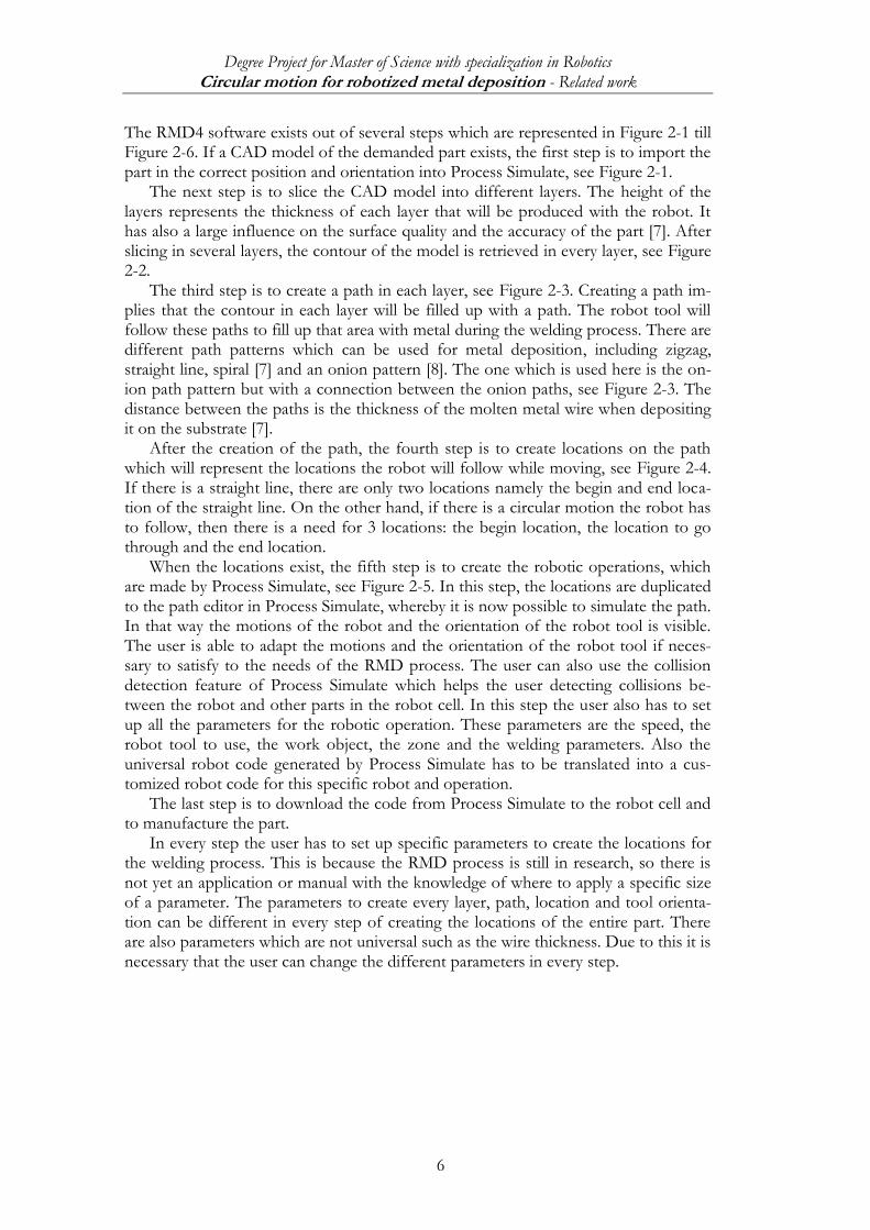
After the creation of the path, the fourth step is to create locations on the path which will represent the locations the robot will follow while moving, see Figure 2-4. If there is a straight line, there are only two locations namely the begin and end loca-tion of the straight line. On the other hand, if there is a circular motion the robot has to follow, then there is a need for 3 locations: the begin location, the location to go through and the end location.
When the locations exist, the fifth step is to create the robotic operations, which are made by Process Simulate, see Figure 2-5. In this step, the locations are duplicated to the path editor in Process Simulate, whereby it is now possible to simulate the path. In that way the motions of the robot and the orientation of the robot tool is visible. The user is able to adapt the motions and the orientation of the robot tool if neces-sary to satisfy to the needs of the RMD process. The user can also use the collision detection feature of Process Simulate which helps the user detecting collisions be-tween the robot and other parts in the robot cell. In this step the user also has to set up all the parameters for the robotic operation. These parameters are the speed, the robot tool to use, the work object, the zone and the welding parameters. Also the universal robot code generated by Process Simulate has to be translated into a cus-tomized robot code for this specific robot and operation.
The last step is to download the code from Process Simulate to the robot cell and to manufacture the part.
In every step the user has to set up specific parameters to create the locations for the welding process. This is because the RMD process is still in research, so there is not yet an application or manual with the knowledge of where to apply a specific size of a parameter. The parameters to create every layer, path, location and tool orienta-tion can be different in every step of creating the locations of the entire part. There are also parameters which are not universal such as the wire thickness. Due to this it is necessary that the user can change the different parameters in every step.
Degree Project for Master of Science with specialization in Robotics Circular motion for robotized metal deposition - Related work
7
2.2 Circular arc algorithm
Curve fitting is an important feature in the analysis of digital curves. Each digital curve exists out of different segments which fit a straight line, a circular arc or a higher or-der curve. That is the reason why straight lines and circular arcs are important features in the field of pattern recognition. Finding these has been a fundamental problem in pattern recognition and image analysis [9]. There are different approaches which have been developed [9], [10-22]. One of the most useful and used techniques for arc or circle detection is based on Hough transform (HT) [10]. HT is mostly used to detect circular patterns from a picture. The Hough Transform converts the pattern recogni-tion problem into a local peak detection by making every point vote for all possible patterns. But HT has several drawbacks, namely it is computational time and memory consuming [10]. Because of these drawbacks variants of the HT have been proposed, including [11], [12].
In this thesis, HT is not a good option because it is time and storage consuming and a fast algorithm is required. Starting from that point of view, other, less complex methods are proposed [9], [13-22]. One of them is vector based [22]. A binary image is vectorized what produces a chain of vectors. After that, there is an attempt to fit the largest possible arc to the curve. It fits a line through the end and the begin vector and calculates then the farthest vector from that line. Then an arc is fitted through these three vectors. After that it calculates the de maximum distance from the remain-ing points to the arc. If this is less than the threshold range, an arc is fitted. In this case the vectorization process is not needed because the locations generated by the RMD4 software are already vectors. On the other hand the method for fitting an arc is a possibility to implement.
Another approach, which is used by some CAD systems, are the Bézier curves [14]. A Bézier curve reduces the amount of locations on a hand drawn spline by ap-proximating the curve with mathematical equations. Out of these equations it gener-ates locations which will represent the curve together with straight lines [13], [14]. This method can highly reduce the amount of necessary locations on a spline, but the locations generated by the Bézier algorithm do not lie on the curve. Because of this, there should be need for an additional step in this thesis to calculate the locations on the curve to represent the midpoint or the location to go through of the circular arc. This makes this method inappropriate for the solution of this thesis.
Another approach is to approximate curves with lines and/or circular arcs [15], [17-19], [21]. The simplest approach under this approximation section is to approxi-mate a curve with a polygon because it fits every digital segment with a straight line [17]. However with the polygonal approach there can be a bigger error to the original curve than with the previous approximation methods. It is also possible to approxi-mate a curve with only circular arcs [18], but then there could be even a higher error to the original curve.
A good approach for approximation a curve for the RMD4 software is that the curve should only exists out of straight lines and circular arcs because then the robot can be programmed with only linear en circular motions. In that way the robot should be easily programmable because the motions in the robot code exist out of linear and circular motion types. If the curve does not exist only out of straight lines and circular arcs, for instance if it exists out of hand drawn curves, then there can be a bigger error on the curve than with the HT or Bézier methods. The approximation of a curve with straight line and circular arcs is a common method because many methods have been

Degree Project for Master of Science with specialization in Robotics Circular motion for robotized metal deposition - Related work
8
proposed to approximate the curve with straight lines and circular arcs, including [9], [15], [20-21].
One possible good method for this thesis is the dynamic focusing approach (DFA) [15]. This method tries to fit a straight line to the entire curve, see Figure 2-7. Then it will calculate the average error from the remaining locations to that straight line, this is represented for one point as a red line in Figure 2-7 till Figure 2-11. If the error is too big, it will try to fit a circular arc to the curve, see Figure 2-8. Then it will calculate the average error from the remaining locations to the circular arc. If this er-ror is too big again, it will shorten the curve with a specific length, in case of Figure 2-9 the length is one, and the algorithm will repeat this until there is a fit with an error which is inside the threshold range, see Figure 2-10. If a positive approximation is detected, the locations of this approximation will be deleted out of the list with loca-tions and the algorithm will restart, see Figure 2-11. This method can achieve a high precision, it is very robust and it is a simple method. The big disadvantage is that it is a very slow algorithm compared to other algorithms including [14].
If, in the DFA algorithm, the curve will be shortened with more than one point, the result will be less accurate, but the method will be faster. The authors of the paper [19] have found a way to improve the accuracy of the approximation with straight lines and circular arcs to the curve in a fast way. It uses two criteria. The first is that it preferences straight lines over circular arcs. The second criterion tries to fit longer lines or arcs instead of many shorter ones.
Another method is based on dominant point detection [16]. The first step is to de-
tect the dominant points. After that it will use arc detection based on chords in tan-gent space to decompose the curve into straight lines and circular arcs. The main ad-vantage of this method is that it is substantially fast.
Figure 2-8 try to fit a circular arc Figure 2-7 try to fit a straight line
Figure 2-9 delete last point Figure 2-10 a circu-lar arc is fitted
Figure 2-11 restart algo-rithm

Degree Project for Master of Science with specialization in Robotics Circular motion for robotized metal deposition - Related work
9
2.3 RMD4 software
The RMD4 software developed at University West is an add-in application to a CAR software [7]. The CAR software which is used in this case is Process Simulate. Process Simulate is used to validate manufacturing processes in a 3D environment. Process Simulate is capable of simulating robotic processes what is needed in this case. Due to the .Net Application Programming Interface (API) which is available, a large portfolio of predefined classes, functions, interfaces, etc. are accessible and/or can be used by add-in applications in Process Simulate. An application programming interface is an interface to communicate in a specific way with a program or between different pro-grams. Using this API, the RMD4 software can run inside Process Simulate. In Figure 2-12 a screen capture of the RMD4 software is taken. In that screen capture, there is a red box with the three windows of the RMD4 software where the user can change the setting to the necessary requirements.
The RMD4 software is a build-on application, which means that it started with a basic program where new features are added until the application has all features and the application is finished.
Figure 2-12 screen capture of the RMD4 software

Degree Project for Master of Science with specialization in Robotics Circular motion for robotized metal deposition - Method
10
3
This thesis consists out of two main goals which were performed side by side. One goal was to search and implement an algorithm to detect circular arcs in a curve and by that way reduce the number of locations.
Potential algorithms were compared to each other and the best suitable for this work has been chosen.
Implement the algorithm in the RMD4 software.
Adapt the algorithm that it works as fast as possible for this purpose.
Debug the algorithm
Test the algorithm on a limited number of different shapes.
Verify the algorithm by: o Test it on shapes were it is known were a circular arc is situated o Check if the algorithm detects the circular arc o Check if the error if inside the given error range o Test it on hand drawn shapes o Check if the error is inside the given error range
The other goal was to verify the RMD4 software and the process from CAD drawing down to robot code. First, it was necessary to have a correct robot cell setup in Process Simulate.
Import robot in Process Simulate
Import the tool frame and work object frame have been imported in Process Simulate by uploading a robotic program from the real robot in Process Simu-late.
Import the tool in Process Simulate
Attach the tool with the correct orientation to the robot
Import a table to represent the not yet used external axis. To verify the RMD4 software and the process from CAD drawing down to robot
code, the following steps were verified on a limited number of different shapes,
Importation of a CAD model
Functions to create a bounding box and the bounding box itself
Slicing the part with the parameters and functions
Path generation with the parameters and functions
Locations creation with the parameters and functions
Create the locations in the path editor in Process Simulate
Download the robot code To test also the next step, so the manufacturing of a part, all these has been done
on a specific part and after that the robot has manufactured the part. When downloading the robot code, Process Simulate generated a universal robot
code. In this case, the robot code gives also instructions for the welding process. To let Process Simulate generate the customized robot code, it was necessary to create offline programming (OLP) files for Process Simulate that change the normal robot code to the customized robot code automatically. OLP is the process in which the
Degree Project for Master of Science with specialization in Robotics Circular motion for robotized metal deposition - Method
11
robot code has been generated without the use of the real robot. Then the OLP files had to be verified:
Create a robotic operation
Test if the OLP files can be read by Process Simulate
Download the customized robot code to the robot
Debug the OLP files by the errors the real robot gives Between the implementation and debugging of the algorithm and the verification
of the process, bugs in the RMD4 software occurred. Some of these bugs were easy to solve and have been solved. Other bugs were too complex to solve in the limited time schedule.
When it was possible to learn more about the RMD process, it became clear that the RMD4 software was missing some important and more user-friendly features. Later on during the project, it was decided to implement some of these missing and more user-friendly features.

Degree Project for Master of Science with specialization in Robotics Circular motion for robotized metal deposition - Circular arc algorithm
12
4
One of the decisive factors for selecting a suited algorithm is their computational time. This is because if the required time to generate the robot path is relatively too long, the RMD4 software becomes impractical towards its usage. The accuracy of approximating a curve is less important than the computational time in this thesis because the RMD process has some errors at its own such as the height of a molten metal droplet [6].
After adding a path to a layer in the RMD4 software, there is already a sort of dominant point detection. Dominant points are points of maximum curvature on a curve; see the green full arc in Figure 4-1. This green full arc line represents the curva-ture of two linear lines which come together in one point and which are composed with points on the curve which are situated between the threshold range represented as striped lines. The dominant points are represented as a rectangular. The circular points are points that will be deleted because they are situated inside the threshold range of a linear line. So the RMD4 software will delete points which are in-between the two end points of a straight line, so the non-dominant points which are represent-ed as circles in Figure 4-1. The dominant points represented as a rectangular in Figure 4-1 are the remaining points. If the points are not on a straight line, then the points are close to each other, dependant on the user defined parameter ‘minimum distance
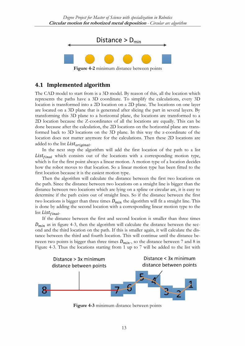
between points’ . The parameter ensures that there are not too many loca-tions on a path by deleting the locations, the circle locations in Figure 4-2, between the two rectangular locations which have a reciprocal distance which is bigger than that parameter. If the distance between two locations after creating a path is smaller
than what is represented by the arrow in Figure 4-2, they will be deleted anyway. From the study of the different algorithms for detecting circular arcs, a variant on
the existing DFA algorithm has been developed in this work [15]. The main algorithm stays the DFA algorithm because it is simple, it can be very accurate and it will fit a straight line’s and circular arcs to a path. The disadvantage is the speed, which has to be fast. Due to this, some changes have been made to the original DFA algorithm especially for the purpose in this case.
Figure 4-1 dominant points
Degree Project for Master of Science with specialization in Robotics Circular motion for robotized metal deposition - Circular arc algorithm
13
4.1 Implemented algorithm
The CAD model to start from is a 3D model. By reason of this, all the location which represents the paths have a 3D coordinate. To simplify the calculations, every 3D location is transformed into a 2D location on a 2D plane. The locations on one layer are located on a 3D plane that is generated after slicing the part in several layers. By transforming this 3D plane to a horizontal plane, the locations are transformed to a 2D location because the Z-coordinates of all the locations are equally. This can be done because after the calculation, the 2D locations on the horizontal plane are trans-formed back to 3D locations on the 3D plane. In this way the z-coordinate of the location does not matter anymore for the calculations. Then these 2D locations are
added to the list .
In the next step the algorithm will add the first location of the path to a list
which consists out of the locations with a corresponding motion type,
which is for the first point always a linear motion. A motion type of a location decides how the robot moves to that location. So a linear motion type has been fitted to the first location because it is the easiest motion type.
Then the algorithm will calculate the distance between the first two locations on the path. Since the distance between two locations on a straight line is bigger than the distance between two locations which are lying on a spline or circular arc, it is easy to determine if the path exists out of straight lines. So if the distance between the first
two locations is bigger than three times the algorithm will fit a straight line. This is done by adding the second location with a corresponding linear motion type to the
list .
If the distance between the first and second location is smaller than three times
as in figure 4-3, then the algorithm will calculate the distance between the sec-ond and the third location on the path. If this is smaller again, it will calculate the dis-tance between the third and fourth location. This will continue until the distance be-
tween two points is bigger than three times ., so the distance between 7 and 8 in Figure 4-3. Thus the locations starting from 1 up to 7 will be added to the list with
Figure 4-3 minimum distance between points
Figure 4-2 minimum distance between points

Degree Project for Master of Science with specialization in Robotics Circular motion for robotized metal deposition - Circular arc algorithm
14
locations . Now the algorithm has detected a path which exists out of loca-
tions which are situated on a spline. The number of locations in the list has
to be at least three otherwise it is not possible to calculate the equation of a circle, neither to make a circular motion with the robot. If there are less than three locations
in the list , it will fit a linear motion to the last location in the list ,
hence it will add that location with a linear motion to the list and it will de-
lete all the locations up to that location which has been added to the list out
of the list . If there are more than three locations in the list, then the algo-
rithm will give to the other part of the algorithm, namely a variant of the
DFA algorithm. The variant of the DFA algorithm was developed in this thesis while debugging the original algorithm to speed up the algorithm and because the original algorithm could in some cases generate wrong approximations which are explained in paragraph 4.3.
The first step of the variant of the DFA algorithm is to take the last and the first
location of and calculate the parameters of a straight line through these loca-
tions. The equation of a straight line is [23],
Where and are the variables of the line and A, B and C are the constants of one specific straight line. The constants of the formula above can be calculated with,
,
and
.
Whereby and are the coordinates of the locations which de-
fines the line. In a special case when , thus when it is a vertical line, the constants can be calculated in following way,
,
and
.
After the equation of the line is calculated, the perpendicular distance of the re-maining locations to the straight line will be calculated. This is calculated in following way [23],
Whereby A, B and C are the values of the straight line and and are the coordi-nates of a location.
After calculating the distance , the algorithm will compare the distance with a maximum error parameter. This parameter is a combination of a user defined parame-ter and the machine error. There are two user defined parameters, which have to be filled in in the parameter list in the graphical user interface of the RMD4 software, one for the fitting precision of a line to a path and another for the fitting precision of
Degree Project for Master of Science with specialization in Robotics Circular motion for robotized metal deposition - Circular arc algorithm
15
a circular arc to a path. Bigger values for these parameters results in less precision of fitting a straight line or circular arc to the path is.
The machine error, also called machine epsilon, is an error which occurs when rounding numbers when calculating [24]. In a calculation rounding occurs because the numerical values have a specific data type. In this case the data type for the numerical values is double. Due to this, the maximum amount of significant figures of a number is sixteen. The machine error is calculated on the biggest value of a coordinate of a location in the list of locations. In that way, the biggest possible machine error is cal-culated.
As soon as the perpendicular distance from one location to the straight line is big-ger than the sum of the machine error and the user defined parameter for linear error, the algorithm cannot fit a line inside the given error range.
If the perpendicular distance of all the locations in list is smaller than the
sum of these two parameters, than the algorithm will add the last location in
with a linear motion type to and will delete all the locations up to the last
location in the list .
If not possible to fit a straight line through the locations in list , the algo-
rithm will try to fit a circular arc through these locations. First it will calculate the equation of the circle through three locations, namely the first, the last and the middle
location in . Three locations are needed because the equation of a circle con-
tains three unknown constants for a specific circle, namely the coordinates of the midpoint of the circle X, Y and the radius R. So there is need to have three different
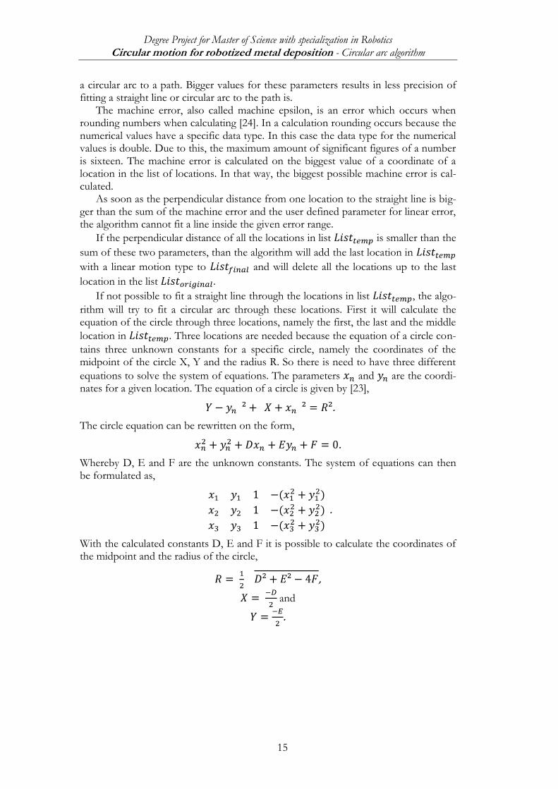
equations to solve the system of equations. The parameters and are the coordi-nates for a given location. The equation of a circle is given by [23],
.
The circle equation can be rewritten on the form,
.
Whereby D, E and F are the unknown constants. The system of equations can then be formulated as,
.
With the calculated constants D, E and F it is possible to calculate the coordinates of the midpoint and the radius of the circle,
,
and
.

Degree Project for Master of Science with specialization in Robotics Circular motion for robotized metal deposition - Circular arc algorithm
16
After the equation of the circle is calculated, the distance between the circle and the locations in the list is calculated. The distance can be calculated by following equation,
.
Where and are the coordinates of a location, is the radius of the circle and
.and are the coordinates of the midpoint of the circle. If this distance is bigger than the sum of the user defined circular error parameter
and the machine error, then it is not possible to approximate the path with a circular arc inside the given error range. If the distance is smaller than the sum of those two parameters, then the algorithm will add the middle and the last location in the list
with a circular motion type to and it will delete the locations up to
the last location in the list .
If a circular motion type is applied to a location, it could appear that some loca-tions have been deleted, for instance the circular orange location in Figure 4-5. Due to this, it is possible that the distance between the new consecutive locations, the two
blue rectangular locations in Figure 4-5, is smaller than . A circular arc fit has been made through the blue rectangular locations in Figure 4-5. Due to this, the circu-lar orange location will be deleted.
Before creating the locations in Process Simulate and after the approximation with linear and circular motion types, the RMD4 software will check if none of the con-secutive locations are too close to each other. In that step it will detect that the two blue rectangular locations of Figure 4-5 are too close to each other. Due to this, the second blue location, where a circular motion type is added on, will be deleted when creating the locations. The removal of a location where a circular motion type is add-ed on may not happen because then there will only be one circular motion type loca-tion instead of two which follows that the robot will not be able to execute the circu-lar motion. This is because a circular motion type needs 2 locations with a circular motion type. Due to this, another function is implemented which is called when a circular motion type will be added to a location.
This new method calculates the distance between consecutive locations whereof one has been fitted with a circular motion type, represented as a blue rectangular loca-
tions in Figure 4-6. If the distance between the locations 1 and 2 is smaller than , it will fit a linear motion to location number 2. After that, the algorithm will delete the
location up to number 2 out of the list and the rest of the path will be ap-
proximated again. If the linear motion should have been added to location number 3 and location
number 2 should have been deleted, a crucial location could have been lost. For in-
Figure 4-6 fitting of linear motion type
Figure 4-5 deleted points

Degree Project for Master of Science with specialization in Robotics Circular motion for robotized metal deposition - Circular arc algorithm
17
stance, if location number 2 should be situated in a corner of the path, the corner should not exist anymore, which can result in another shape of the path.
If it was not possible to fit an arc or a line through the given locations, then the
last location will be deleted out the list and the process will start again by
trying to fit a straight line through the resulting locations. This process will continue until an approximation by a linear line or circular arc was possible. Then these loca-
tions will be deleted out of the list and the specific location(s)will be added
to the list with the corresponding motion type. Further the algorithm will
start over with the resulting locations in the list . This process will continue
until the list is empty. As soon as the list is empty, the entire
curve is approximated with linear lines and circular arcs. This process can also be fol-
lowed in Figure 2-7 up to Figure 2-11. After the list does not contain any
locations anymore, the list contains the resulting locations on the path with
the corresponding motion type. If the robot needs to complete an entire circle, then it needs in theory 3 locations
which define the circle. In this case the robot processes a welding operation whereof one parameter is the overlap distance. This user defined parameter lets the user decide how big the distance is for the overlap on the onion path, as shown in Figure 4-7. Due to this overlap distance, the circular motion can be more than 360 degrees. This means that the robot will not execute the correct motion, it will execute a motion less than 360 degrees in the opposite direction instead of more than 360 degrees in the correct direction. Due to this, it is necessary to split up the circular motion of more than or equal to 360 degrees into several pieces. In this thesis, a circular motion of less than 90 degrees exists out of one circular motion. If the angle is more than 90 degrees and less than or equals to 180 degrees is divided into two equally spaced circular mo-tions. If it is more than 180 and less than or equals to 270 degrees, it is divided into three equally spaced circular motions. If it is more than 270 degrees, it is divided into four equally spaced circular motions. This is necessary for the welding process for the reason that the welding parameters have to be changed in every circular motion. This property was also imposed by GKN.
The first step in the method to calculate the angle of the circular motion is to cal-culate the angle between the first location and the middle location of the circular mo-tion. Then the angle is calculated between the middle location and the last location of the circular motion. These two angles are added to each other and represent the total angle of the circular motion.
Figure 4-7 overlap dis-tance

Degree Project for Master of Science with specialization in Robotics Circular motion for robotized metal deposition - Circular arc algorithm
18
The angle is not calculated immediately between the first and the last location of the circular motion because the angle between those two can be more than 360 de-grees. If the angle would be calculated in this way, the angle should be smaller than 360 degrees. In that way, it would be impossible to detect if a circular motion is more than 360 degrees.
A simplified flow chart of the implemented algorithm can be found in Appendix A. It contains the major steps of the algorithm.
4.2 Extra acknowledge
Not every location on the path is known from the beginning, because the locations between the two end locations of a straight line already have been deleted. As a result of the reduced information on locations, the algorithm can generate sometimes wrong results. For instance if the resulting locations of a path would exist out of three points which are lying on three corners of a rectangular, see Figure 4-8, then the original DFA would fit a circular arc between these locations. This is because the algorithm first would try to fit a straight line between these three locations, which would fail because the distance from the middle locations to the line would be too large. Then it would try to fit a circular motion that would fit because the algorithm will fit a circle through the three locations and in Figure 4-8 there are only 3 locations. So a circular motion would be fitted to these locations, what would be wrong. Due to this, it is necessary to have first the small function, which checks if the distance between the
locations is bigger or smaller than three times , before calling the customized DFA algorithm.
Due to this first small algorithm, the customized DFA algorithm will detect very quickly if there is an approximation by a straight line or a spline. So it will not try to fit a straight line through the entire path, but only to the locations which distance is big-
ger than three times . This is the main optimization if it comes up to the speed of the algorithm. The implemented algorithm will be much faster than the original algorithm if the path exists out of alternately straight lines and splines. In case that the path only exists out of splines and different circular arcs, the speed will be comparable with the original DFA algorithm.
The parameter to determine if the distance between two locations is large or small
is three times . There is no existence of a parameter which declares the maxi-mum distance between two locations. On the other hand is the distance between two
locations dependent of the parameter . It is multiplied with three because out of several tests this seemed the best numerical value.
Figure 4-8 fitting of circular motion instead
of linear motion

Degree Project for Master of Science with specialization in Robotics Circular motion for robotized metal deposition - Circular arc algorithm
19
4.3 Implementation of extra features
Because this application is an ongoing project which ends when the software consists all the features and is completely debugged, it was possible to continue working and to implement extra features into the application.
4.3.1 Extra features for the circular motion algorithm
To start the convert to circular motions algorithm, a button is needed in the RMD application. Due to this, a ‘convert to circular motion’ button is implemented. If the user clicks this button, the list with all the locations will be changed to a list with nor-mally less locations and motion types connected to every location. The user does not see the new locations yet. To represent the new locations on the screen, the user must click the already existing ‘create locations’ button. After clicking that button, the result of the convert to circular motion algorithm will be visible.
Now every location has a specific motion type, namely linear or circular. The user can easily see if a location has a circular or linear motion type due to the icons next to every location which represents a motion type, see Figure 4-9. In the visualization of the locations in Process Simulate the colors of the frames for a linear and circular motion type has been given a different color, see Figure 4-10. In that way the user can also easily see where the robot will execute a circular motion type.
If the obtained result is not the desired result, the user should be able to change the motion type of every location. Due to this, two new buttons are implemented, one button to convert the motion type to a circular motion and one to change the motion type to a linear motion. In that way the user is able to select one or more locations and change the motion type from these locations to another motion type.
If the user is not satisfied with the result after changing to circular and linear mo-tions, the user should be able to go back to the starting point with all the locations on the path. Because of this, a new button is implemented, namely ‘Restore original loca-tions’. This button changes the locations back to the original locations with only linear motion types. Now the user is able to start over again.
Because the algorithm needs some time to calculate the fitting of linear and circu-lar motions, it is useful that the user can see if the algorithm is working or not. Due to this, a text line has been added to the status bar of Process Simulate where it is shown if the algorithm has finished or not.
Figure 4-9 new icons Figure 4-10 coloured frames
Degree Project for Master of Science with specialization in Robotics Circular motion for robotized metal deposition - Circular arc algorithm
20
4.3.2 Implementation of a function for new locations
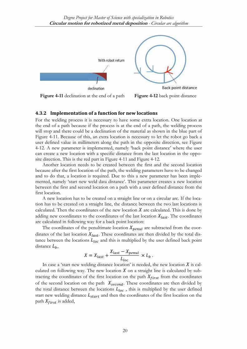
For the welding process it is necessary to have some extra location. One location at the end of a path because if the process is at the end of a path, the welding process will stop and there could be a declination of the material as shown in the blue part of Figure 4-11. Because of this, an extra location is necessary to let the robot go back a user defined value in millimeters along the path in the opposite direction, see Figure 4-12. A new parameter is implemented, namely ‘back point distance’ where the user can create a new location with a specific distance from the last location in the oppo-site direction. This is the red part in Figure 4-11 and Figure 4-12.
Another location needs to be created between the first and the second location because after the first location of the path, the welding parameters have to be changed and to do that, a location is required. Due to this a new parameter has been imple-mented, namely ‘start new weld data distance’. This parameter creates a new location between the first and second location on a path with a user defined distance from the first location.
A new location has to be created on a straight line or on a circular arc. If the loca-tion has to be created on a straight line, the distance between the two last locations is
calculated. Then the coordinates of the new location are calculated. This is done by
adding new coordinates to the coordinates of the last location . The coordinates are calculated in following way for a back point location:
The coordinates of the penultimate location are subtracted from the coor-
dinates of the last location . These coordinates are then divided by the total dis-
tance between the locations and this is multiplied by the user defined back point
distance ,
In case a ‘start new welding distance location’ is needed, the new location is cal-
culated on following way. The new location on a straight line is calculated by sub-
tracting the coordinates of the first location on the path from the coordinates
of the second location on the path . These coordinates are then divided by
the total distance between the locations , this is multiplied by the user defined
start new welding distance and then the coordinates of the first location on the
path is added,
Figure 4-11 declination at the end of a path Figure 4-12 back point distance

Degree Project for Master of Science with specialization in Robotics Circular motion for robotized metal deposition - Circular arc algorithm
21
.
Another possibility is that the location has to be created on a circular arc. To sim-plify the calculations, the coordinates of the locations are first transformed into 2D locations. Then the equation of the circle is calculated. Due to this the coordinates of
the midpoint and and the radius of the circle is known. Then the angle that the new location has to make relative to the last location is calculated with the follow-ing formula [23],
which follows that
.
The next step is to calculate the angle between the last location and the x-axis . The resulting angle is obtained by subtracting the angle between the x-axis and the last
location with the calculated angle , as shown in Figure 4-13,
.
The coordinates of the new location can be calculated with the following formula,
and
.
In that way the new coordinates of the back point location are known and the lo-cation can be created. The last step is to transform the 2D locations back to 3D loca-tions.
If the location is a ‘start new welding distance location’ and has to be created on a circular arc, the formulas are the same as for a ‘back point’ location except for the
formula to calculate . In this case the angle is obtained by adding the angle between
the x-axis and the first location with the calculated angle ,
.
The motion to go to these locations is always linear. This is because the user re-quired distance will always be small according to the total size of the path. In that way is the difference between a linear motion and a circular motion negligible.
Figure 4-13 back location

Degree Project for Master of Science with specialization in Robotics Circular motion for robotized metal deposition - Setting up the robot cell in Process
Simulate
22
5
A correct robot setup in Process Simulate from the real robot cell is necessary to gen-erate the correct robot code. This is because the robot code is dependent on a lot of real parameters including the robot, the RCS version of the server, the tool and the work object.
The robot is the base of the whole welding operation. Every robot has a different manufacturer, a different length of axis, can lift different weights, the maximum rota-tion of the axis’s are different and many more. Because of this reasons it is necessary to have the correct robot in Process Simulate. The robot in this robot cell is an ABB robot with the specifications IRB 4400, 60kg and 1,96m. Also the orientation of the robot relative to the external axis in Process Simulate has to be correct otherwise the robot code will not be correct.
To have the correct frames out of the real robot cell in Process Simulate, a pro-gram from the real robot was uploaded to Process Simulate. In that way, the frames were added into Process Simulate with the correct coordinates and orientation. The frames which were imported are the work object frame and the tool frame.
The tool frame is in this case a virtual point. It is the point where the laser beam and the metal wire come together. The tool frame is an offset from the mounting flange of the robot.
The work object frame is a frame from which the coordinates of the locations of the part are relative to. For example, if the work object frame moves 100 in X direc-tion, then the coordinates of the locations of the part will also move 100 in X direc-tion. Next to X,Y and Z coordinates, the work object frame also contains the orienta-tion of the tool frame relative to the work object frame. After importing those frames into Process Simulate, the orientation of the tool frame was exactly the same as the orientation of the work object frame. This was not correct because the orientation parameter (quaternion) in the work object frame were not [1,0,0,0], which would rep-resent that there is no rotation. Due to this, there had to be a rotation of the tool frame relative to the work object frame. Also when the robot moved along the x-axis of the work object frame, the direction was different of when moving along the x-axis of the tool frame.
The quaternion of the work object is: [0.720221, 0.001032, 0.001897, 0.693741]. The last three numbers represent the unit vector which about to rotate. The first number is the rotation angle. Because the second and third number is much smaller than the last number, these two can be ignored so that there is only a rotation around
the Z-axis. Then the rotation angle is calculated: which fol-
lows that [25]. This rotation around the Z-axis was manually imported in Process Simulate. When downloading a location created by Process Simulate to the robot, the robot tool orientation was correct. This means that the calculated rotation angle was correct. The rotation of the tool relative to the work object frame is shown in Figure 5-1. The white frame is the rotation of the tool; the wire feeder’s orientation is the Y-axis of the work object.

Degree Project for Master of Science with specialization in Robotics Circular motion for robotized metal deposition - Setting up the robot cell in Process
Simulate
23
To see the simulated process properly, the tool, see Figure 5-2, is also an im-portant feature. The real tool in the robot cell is too complicated to replicate, because there are many features mounted on the tool which are only necessary to investigate the welding process. The features which are needed in this case are the wire feeder and the laser beam. These two parts are from a manufacturer from who the correct CAD drawings are available. The assembly of the parts on the robot is custom made whereby there is no correct information available. This is the reason why the tool does not fit properly on the mounting flange of the robot in Process Simulate. This is not a problem because the mounting of the tool is not important. It is necessary that the point where the metal wire and the laser beam of the tool come together, the TCP, has the same location as the tool frame uploaded into Process Simulate from the real robot. In that way it is possible to detect collisions with the collision detection feature in Process Simulate. Also if the user wants to rotate the tool in a specific way, the tool will be rotated around the TCP. When simulating the process, it is important to see how the tool moves while manufacturing the part, which is now possible.
In the robot cell there is an external axis. Because this external axis is not in use yet, there is no meaning to import the external axis in Process Simulate. Instead of the external axis, a simple table is placed in the same position. The robot setup is illustrat-ed in Figure 5-3.
Figure 5-2 tool Figure 5-1 tool frame
Figure 5-3 robot cell setup

Degree Project for Master of Science with specialization in Robotics Circular motion for robotized metal deposition - Setting up the robot cell in Process
Simulate
24
5.1 Implementation of download script
The real robot has its own custom robot code, so it is necessary to write a custom script that changes the normal robot code generated by Process Simulate to a custom-ized robot code. An example of the original and the customized robot code in this case is shown in appendix B.
The welding process needs some additional locations and information, see Figure 4-13. Due to this, some extra features had to be implemented to test the robot code on the real robot. When starting the process, the robot has to approach the first loca-tion of the path slowly, so a location can be created before the first location on the path with a Z offset and eventually a X or Y offset. A button is implemented that adds such a location.
The next location is the first location on the path where the welding process will start. To start a welding operation, custom commands and parameters are needed. The normal code which will be printed out by Process Simulate uses MoveL and MoveC instructions for a motion type. Because an ABB robot is used, the instruction for a linear motion is MoveL and for a circular motion MoveC. Because the welding operation has to start in the first location and the welding parameters are given by the robot code, there is need to change the standard instructions to customized instruc-tions. On the first location, the name of the motion type needs to have the name ‘MDL\MDLOn’ for a linear motion type and ‘MDC\MDCOn’ for a circular motion type. This command enables the laser.
In the same location, the laser has to be started. Due to this a button is created which adds an instruction after the laser on instruction in the robot code. The MoveL or MoveC motion type names are changed into MDL\MDLStart for a linear motion type and MDC\MDCStart for a circular motion type. It does not create a new loca-tion in the Path Editor in Process Simulate, but it only prints out an extra line with the instructions in the robot code. After the user has clicked the button, what will be printed out is visible in the ‘OLP commands’ table.
After the laser has been started and before the laser has been stopped, all the mo-tion type names are the same, namely MDL for a linear motion type and MDC for a circular motion type. The change of the motion type name from MoveL to MDL and from MoveC to MDC is done automatically when generating the robot code.
On the last location of the welding operation, the laser has to be stopped. In that location the name of the motion type will be changed to ‘MDL\MDLStop’ for a line-ar motion and ‘MDC\MDCStop’ for a circular motion.
In the same location, the laser has to be switched off. A button is implemented that adds this instruction after the stop instruction in the robot code. The printed out motion type name is MDL\MDLOff or MDC\MDCOff dependent on the motion type. After the user has clicked the button, it is visible in the ‘OLP commands’ what will be printed out.
To end a path, it is good that the robot moves to an end location which is situated higher than the last location. In that way the metal wire will not be stuck to the depos-ited metal on the substrate. To generate a new location, a button is implemented that creates a new location as last location with a Z and X or Y offset.
Before and after the welding process, the robot has to communicate with other devices. Due to this, just after every PROC and just before ENDPROC, except for the main procedure, some lines of specific text are added.
As mentioned above, there are different weld data’s. The user first has to define the different weld data’s in Process Simulate required for the welding process. After

Degree Project for Master of Science with specialization in Robotics Circular motion for robotized metal deposition - Setting up the robot cell in Process
Simulate
25
that, the user can add a defined weld data to a specific location as required. Also a new column has been created in the Path Editor in Process Simulate where the user can follow the weld data on every location. This specific weld data is also printed out in every instruction.
To let other users use these new functions and buttons, a manual was written of how to use the new buttons. To let programmers understand the structure of the off-line programming files so that it is easy to adapt the files, the structures of the xml files was explained in a manual.

Degree Project for Master of Science with specialization in Robotics Circular motion for robotized metal deposition - Results and discussion
26
6
In the next paragraphs the results of the implemented circular arc algorithm and the verification of the entire process will be expounded.
6.1 Circular arc algorithm
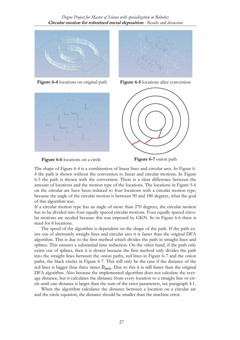
The algorithm for approximating a path with circular arcs and straight lines has been tested and the results were satisfactory. Different shapes have been tested, including an egg shape as in Figure 6-1. This kind of shape is a hand drawn shape where it was not possible to predict where the algorithm would fit linear and circular motion types. Also shapes where it was known in advance where the algorithm should fit a linear and circular motion type have been tested as in Figure 6-4, the same shape but with larger dimensions and a circle as in Figure 6-6. In that way it was possible to verify the algorithm. In Figure 6-1 and Figure 6-2 a conversion to circular and linear motions is visible with the value of the parameters for linear and circular error on 0 mm. The number of locations has been reduced from 222 locations down to 33 locations; also the motion types have been changed from only linear in Figure 6-1 to linear and circu-lar in Figure 6-2. The algorithm has fitted the different motion types within the given error range what was the purpose. In Figure 6-3 the parameter for linear motion error has been changed to 1 mm, which gives a result with more linear motions.
Figure 6-1 original path with 222 locations
Figure 6-2 path after converting, 33 locations left
Figure 6-3 linear error = 1mm
Degree Project for Master of Science with specialization in Robotics Circular motion for robotized metal deposition - Results and discussion
27
The shape of Figure 6-4 is a combination of linear lines and circular arcs. In Figure 6-4 the path is shown without the conversion to linear and circular motions. In Figure 6-5 the path is shown with the conversion. There is a clear difference between the amount of locations and the motion type of the locations. The locations in Figure 5-6 on the circular arc have been reduced to four locations with a circular motion type, because the angle of the circular motion is between 90 and 180 degrees, what the goal of this algorithm was. If a circular motion type has an angle of more than 270 degrees, the circular motion has to be divided into four equally spaced circular motions. Four equally spaced circu-lar motions are needed because this was imposed by GKN. So in Figure 6-6 there is need for 8 locations.
The speed of the algorithm is dependent on the shape of the path. If the path ex-ists out of alternately straight lines and circular arcs it is faster than the original DFA algorithm. This is due to the first method which divides the path in straight lines and splines. This ensures a substantial time reduction. On the other hand, if the path only exists out of splines, then it is slower because the first method only divides the path into the straight lines between the onion paths, red lines in Figure 6-7 and the onion paths, the black circles in Figure 6-7. This will only be the case if the distance of the
red lines is bigger than three times . Due to this it is still faster than the original DFA algorithm. Also because the implemented algorithm does not calculate the aver-age distance, but it calculates the distance from every location to a straight line or cir-cle until one distance is larger than the sum of the error parameters, see paragraph 4.1.
When the algorithm calculates the distance between a location on a circular arc and the circle equation, the distance should be smaller than the machine error.
Figure 6-4 locations on original path
Figure 6-7 onion path
Figure 6-5 locations after conversion
Figure 6-6 locations on a circle
Degree Project for Master of Science with specialization in Robotics Circular motion for robotized metal deposition - Results and discussion
28
In this case that distance is in average the machine error multiplied with 1015. This is because the process from CAD model down to robot code undergoes a lot of steps and calculations whereby there pile a lot of errors. An error is made when visualising a CAD model in Process Simulate. The visualisation of a circular arc is not circular, but it exists out of straight lines which are connected with each other to represent a circu-lar arc. When slicing the part, there will also be an error on these sections. When cal-culating the locations on the path, there will be an error as well.
Because there is already an error in the begin stage, the error will incur with every step. Due to all the errors together, it is necessary that the distance from a location to the straight line or circular arc is smaller than an empirical error value. This empirical error value is the machine error multiplied with a factor 1014+log(largest size), with the larg-est size is the largest dimension of the X or Y coordinates of one location on a path. The empirical factor was found by testing a specific part with different sizes. If the size was between 0 and 10, a value from 0 till 1 had to be added to the factor 1014. If the size was between 10 and 100, a value from 1 till 2 had to be added to the factor 1014. This can be continued. In that way it was possible to take the logarithm from the biggest size of a part to calculate every time the error.
If the user is not satisfied with the result obtained with this error, the user can al-ways enlarge or reduce the circular error parameter to obtain another, more satisfacto-ry result. In that way the developed algorithm is very flexible.
6.2 Verification of the process from CAD drawing to robot code
Importing a CAD model in jt format, which is the standard format for Process Simu-late, does not give any problems.
The next step is to add a robot, part and parameter file to the RMD4 software. In that way the RMD4 software knows what to use for the path creation. Neither this gives a problem.
Then a bounding box needs to be created around the part. A bounding box is a box with the smallest volume wherein all the points of a part are situated. If the dis-tances between the planes of the part and the planes of the bounding box are meas-ured, the distance is always positive. This means that the part lies totally inside the bounding box, what is the requirement of a bounding box.

Degree Project for Master of Science with specialization in Robotics Circular motion for robotized metal deposition - Results and discussion
29
After creating a bounding box, the part has to be sliced into different layers. If the shape of the part where the first layer has to be created is flat, then the first layer is correct. If it is not flat but curved, then the first layer is not correct. In Figure 6-8 is a part shown whereof the surface is curved. The first layer which is created is the lowest green line, the second layer, which is correct, is the green oval above. In theory, two islands should have been created to form the first curved layer, but this is not the case. It is also possible that the location of the bounding box frame should be located in the lowest part of the part. It is too difficult to locate that frame exactly in that point. Due to this, improvement is needed. Starting from the second layer, every layer is correct.
The next step is to add a path to a layer. This step works sometimes, but in several cases it does not work. If the shape of a path is correct or not, depends most of the time on the value for the parameters ‘Path_ContourOffset’ and ‘Path_PathWidth’. So there is no specific case in which this step works or in which it does not work. An example is shown in Figure 6-9. Sometimes it also creates two paths, whereof one is the correct one and the other is completely wrong. Sometimes it is even located out-side the bounding box, see Figure 6-10. When the value of the parameter ‘Path_contourOffset’ was zero, the RMD4 software arrived in an infinite loop. This problem has been solved by adding a case if the value is zero. The user has also the possibility to choose if the part is manufactured from the outside to the inside or the other way around. This function didn’t work, but has been solved. The generation of a path gives the most problems in the RMD4 software. This function still has some substantial bugs which need to be debugged urgently for a usable RMD4 software.
After creating the path, the locations have to be created. Before creating the loca-tions, the user can convert the locations to linear and circular motions what works as described in paragraph 5.1. The converting back to only linear motions also works because then all the locations are back on the path as in the beginning. The buttons for changing a location to circular or linear motion type works as well. In that case, the icon in front of the name of the location changes, what is the purpose. If one cre-ated location is not correct, the user should be able to delete that location. This step did not work but has been debugged.
Before creating the locations, the tool frame had to be selected so that the frame of the locations has the same orientation as the tool frame. This is necessary because the tool frame orientation will follow the orientation of the locations. If the locations are created, the orientation of the locations is the same as the orientation of the tool frame. It is also possible, for instance in case of a cylinder, that the frame of a location
Figure 6-8 curved surface
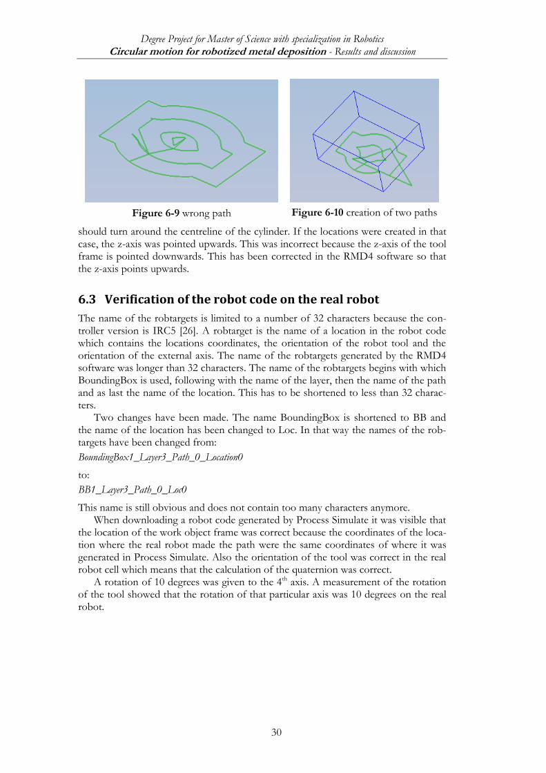
Degree Project for Master of Science with specialization in Robotics Circular motion for robotized metal deposition - Results and discussion
30
should turn around the centreline of the cylinder. If the locations were created in that case, the z-axis was pointed upwards. This was incorrect because the z-axis of the tool frame is pointed downwards. This has been corrected in the RMD4 software so that the z-axis points upwards.
6.3 Verification of the robot code on the real robot
The name of the robtargets is limited to a number of 32 characters because the con-troller version is IRC5 [26]. A robtarget is the name of a location in the robot code which contains the locations coordinates, the orientation of the robot tool and the orientation of the external axis. The name of the robtargets generated by the RMD4 software was longer than 32 characters. The name of the robtargets begins with which BoundingBox is used, following with the name of the layer, then the name of the path and as last the name of the location. This has to be shortened to less than 32 charac-ters.
Two changes have been made. The name BoundingBox is shortened to BB and the name of the location has been changed to Loc. In that way the names of the rob-targets have been changed from:
BoundingBox1_Layer3_Path_0_Location0
to:
BB1_Layer3_Path_0_Loc0
This name is still obvious and does not contain too many characters anymore. When downloading a robot code generated by Process Simulate it was visible that
the location of the work object frame was correct because the coordinates of the loca-tion where the real robot made the path were the same coordinates of where it was generated in Process Simulate. Also the orientation of the tool was correct in the real robot cell which means that the calculation of the quaternion was correct.
A rotation of 10 degrees was given to the 4th axis. A measurement of the rotation of the tool showed that the rotation of that particular axis was 10 degrees on the real robot.
Figure 6-9 wrong path Figure 6-10 creation of two paths

Degree Project for Master of Science with specialization in Robotics Circular motion for robotized metal deposition - Conclusion
31
7
New features have been implemented in the RMD4 software. The circular motion algorithm has proven to be accurate, dependent on the user defined parameters, and it is substantially fast. Due to the big errors on the locations in Process Simulate and the RMD4 software while calculating the locations, the user sometimes has to adapt the linear and circular error parameters to attain the required approximation of the path.
The RMD4 software has been tested on every step. The bugs which appeared dur-ing the testing of the RMD4 software have been written in a word file with the expla-nation and a picture of what was generated wrong.
A path generated by the application has been downloaded to the robot and the robot in the robot cell moved along the path. This means that the robot setup in Pro-cess Simulate is correct and what has been generated by the off line programming files is also correct.
The final conclusion of this thesis is that the goals have been reached and the work done is approved. The RMD4 software is improved substantially. Despite the work done, some features in the RMD4 software needs to be debugged more and some extra features are needed to reach a good user-friendliness.
7.1 Future Work and Research
The application still misses some valuable features. It should be good if it is possible to copy a complete layer to another layer. In that way, the user does not have to make a layer over and over again if the data for these layers is all the same except for the coordinates of the locations which will have an offset in the building direction.
At this moment, the robot tool can change its orientation along the path. But this change is only possible for the entire path, what is not a requirement in every case. The user should be able to do this only for some user required locations. This could be good for the welding process because then a higher percentage of the laser energy could go into the part. Also a more accurate manufactured part and a higher surface quality could be obtained. To improve this, a function should be implemented in the RMD4 software so that the user can select a number of locations around which the tool should rotate over a user defined amount of degrees relative to the path.
Now the user has only the possibility to generate an onion path. In the future the user should be possible to choose between different kinds of paths.
In the current RMD4 software it is only possible to generate a path on a flat sur-face. In the future it should be possible to generate a path on a curved surface.
The user-friendliness of changing the robot code, generated by Process Simulate to the customized robot code has to be improved. Now the user still has to click on many buttons. Also this should be able to copy from one layer to another.
To do this, it is perhaps easier to add a new window to the RMD4 software where the user can set every robot setup variable, including the weld data, tool data, work object data, speed data, zone data and process type (MDLOn, MDL, and MDLStop). In that way the user will be able to copy layers in the RMD4 software with all the re-quired variables. When the user then creates the robotic operations, everything will be

Degree Project for Master of Science with specialization in Robotics Circular motion for robotized metal deposition - Conclusion
32
filled in in the path editor in Process Simulate. The only thing left to do for the user is to check the robotic operation, the collision detection and to change the parameters where necessary. This should be a big improvement of the user-friendliness pertaining to the current process of generating the customized robot code.
7.2 Critical Discussion
The implemented algorithm to approximate a path with linear lines and circular arcs is approved. The solution for the error if a location is on a linear line or circular arc is only an empirical solution. The error should be more investigated so that the empiri-cal value can be modified into a more founded solution. Also it should be positive if the origin of the errors should be more investigated. In that way it could be possible to minimize the error and to have a more accurate result.
The implementation of the extra features took only a small fraction of the availa-ble time. The RMD4 software should have been more improved if the path creation bug should have been solved. Due to the limitation of time it was not possible to in-dulge in the algorithm of the path creation. Because of this, the choice to implement some new features to the RMD4 software has been made.
As a result of this thesis, I have learned a new programming language and my pro-gramming skills are improved a lot. Also I learned how to work with robots and how to offline program robots. I gained knowledge about the RMD process from which I had never heard of. In conclusion this thesis was a great and instructive experience.
7.3 Generalization of the result
The algorithm in this study is specific developed for the RMD process and the already existing features in the RMD4 software. Think about the already built-in dominant point detection. But the developed algorithm is a general algorithm which can be used to approximate a curve with linear lines and circular arcs.
The verification of the process from CAD drawing down to robot code in only applicable in this specific case because the tool is custom made, one specific robot is used, and more. The verification of the RMD4 software is only applicable on the RMD4 software so this is specific again.
On the other hand, the developed files which are created to let Process Simulate generate a customized robot code are universal if used by Process Simulate. Any type of robot code customization can be obtained with these files. But the content of the customised robot code is only applicable in this specific case.
With some extra functions, the RMD4 software can be used to generate a robotic operation for every kind of process which involves that the robot has to follow a spe-cific path defined by a CAD model. An example in this case is thermal spray where the robot has to follow the outer contour of the CAD model.
Degree Project for Master of Science with specialization in Robotics Circular motion for robotized metal deposition - References
33
8
[1] M. Ericsson, F. Danielsson, H. Carlsson, P. Nylén, “Off-line programming of robots for metal deposition.”, Pine Mountain, Georgia: Trends in welding re-search: Proceedings of the 7th international conference, pp. 629 – 634, 2005.
[2] H. K. Dyavaiah, “Design & Implementation of RMDLib in Process Simulate for RMD.”, University West, Department of Engineering Science, 2008.
[3] H. Carlsson, “Implementation of a robot tool path creation application for robotized metal deposition.”, University West, Department of Technology, Mathematics and Computer Science, 2005.
[4] K. M. B. Taminger, R. A. Hafley, “Electron beam freeform fabrication: a rap-id metal deposition process.”, Proceedings of the 3rd Annual Automotive Composites Conference, September 9-10, Troy, MI. Society of Plastics Engineers, 2003.
[5] Y. Zhang, Y. Chen, P. Li, A. T. Male, “Weld deposition-based prototyping: a preliminary study.”, Journal of Materials Processing Technology 135, pp. 347-357, 2003.
[6] A. Heralic, “Towards full Automation of Robotized Laser Metal-wire Deposi-tion”, Chalmers University of Technology, Department of Signals and Sys-tems, 2009.
[7] E. Glorieux, J Cobbaert, “Development of an application for offline pro-gramming of the process of robotized metal deposition.”, University West, Department of Engineering Science, 2011.
[8] Björkqvist, “Implementation and validation of onion path pattern for RMD.”, University West, Department of Engineering Science, 2010
[9] B. Sarkar, L. K. Singh, D. Sarkar, “Approximation of digital curves with line segments and circular arcs using genetic algorithms.”, Pattern Recognition Letters 24, pp. 2585 – 2595, 2003.
[10] H. Kälviäinen, P. Hirvonen, L. Xu, E. Oja, “Probabilistic and non-probablistic Hough transform: overview and comparisons.”, Image and Vision Computing, Vol. 13 No. 4 May 1995, pp. 239 – 252
[11] L. Xu, R. Oja, P. Kultanan, “A new curve detection method: Randomized Hough Transform (RHT).”, Pattern Recognition Letters 11, pp.331 – 338, 1990.
[12] S.-H. Chiu, J.-J. Liaw, K.-H. Lin, “A fast randomized transform for cir-cle/circular arc recognition.”, International Journal of Pattern Recognition and Artifi-cial Intelligence ,Vol. 24, No. 3, pp. 457-474, 2010.
[13] Y.J. Ahn, H.O. Kim, “Approximation of circular arcs by Bézier curves.”, Jour-nal of Computational and Applied Mathematics 81, pp. 145 – 163, 1997.
[14] S.-H. im, Y.J. Ahn, “An approximation of circular arcs by quartic Bézier curves.”, Computer-Aided design 39, pp. 490 – 493, 2007.
[15] C. Ichoku, B. Deffontaines & J. Chorowics, ‘’Segmentation of digital plane curves: A dynamic focusing approach.”, Pattern Recognition Letters 17, pp. 741 – 750, 1995.
[16] T. P. Nhuyen, I. Debled-Rennesson, “Decomposition of a curve into arcs and line segments based on dominant point detection.”, Scandinavian Conference on Image Analysis, 2011.

Degree Project for Master of Science with specialization in Robotics Circular motion for robotized metal deposition - References
34
[17] J. Hu, H. Yan, “Polygonal approximation of digital curves based on the prin-ciples of perceptual organization.”, Pattern recognition, Vol. 30, No. 5, pp. 701 – 718, 1997.
[18] S-C. Pei & J-H. Horng, “Fitting digital curve using circular arcs.”, Pattern Recognition 28 (1), pp. 107 – 116, 1995.
[19] J.-H. Horng, J. T. Li, “A dynamic programming approach for fitting digital planar curves with line segments and circular arcs.”, Pattern Recognition Letters 22, pp. 183-197, 2011.
[20] J.-H. Horng, “An adaptive smoothing approach for fitting digital planar curves with line segments and circular arcs.”, Pattern recognition letters 24, pp. 565 – 577, 2002.
[21] H.-T. Sheu, Member, IEEE, W.-C. HU, “Multiprimitive Segmentation of Pla-nar Curves-A Two-Level Breakpoint Classification and Tuning Approach.”, IEEE transactions on pattern analysis and machine intelligence, Vol. 21, No. 8, pp. 791 – 797, 1999.
[22] D. Elliman, “Arc segmentation in Engineering drawings.”, University of Not-tingham UK, Computer Science Technical Report No. NOTTCS-TR-2001-1, 2001.
[23] J. W. Harris, H. Stocker, Handbook of Mathematics and Computational Science. New York: Springer-Verlag, 1998.
[24] R. J. Schilling, S.L. Harris, Applied Numerical Methods for Engineers: Using Matlab and C. Pacific Grove, CA 93950 USA: BROOKS/COLE PUBLISHING COÖPANY, 2000.
[25] D. Eberly, “Quaternion Algebra and Calculus.”, geometrictools.com , 2 March 1999. [Online]. Available: http://www.geometrictools.com/Documentation/Quaternions.pdf. [Visited on the 18th of April 2013].
[26] ABB Robotics, Technical reference manual - RobotWare 5.12, 2004 - 2009.

Degree Project for Master of Science with specialization in Robotics Circular motion for robotized metal deposition - Flow chart of the algorithm
Appendix A:1
A.

Degree Project for Master of Science with specialization in Robotics Circular motion for robotized metal deposition - Customized robot code
Appendix B:1
B.
In this appendix the original robot code and the customized robot code are shown. It is visible that the data types have been changed: two new data type has been created, namely laser weld data and num data. The laser weld data is the data which is necessary for the RMD process. The num data is needed so that the robot can show which path it is manu-facturing. The zone data has been deleted because this data is not used by the process.
The biggest change is visible if the robot motion types. The move instructions for exe-cuting the RMD process have been changed to customized motion types. When a MoveL or MoveC is visible in the robot code, it means that the RMD process is not executed yet.
Also an extra data type has been added to the instructions, namely the laser weld data, which is in this case startWeldData and nominalWeldData.
Two buttons have been created in the path template action in Process Simulate to add an approach location as the first location and an end location as the last location to a path.
Finally, after every PROC, before every ENDPROC and sometimes after a location, a couple of text lines have been added. This was needed for the computers which are observ-ing the RMD process and to let the user know what the robot is doing at a specific time.
Beneath, first the original robot code and secondly the customized robot code is shown.
Original robot code:
!# ----------------------------------------------
!# ------ ROBTARGET
!# ----------------------------------------------
LOCAL CONST robtarget BB1_Layer3_Path_0_Loc0_app:=[[-125.956695,236.145817,-
16.828602],[0.032768,-0.355247,-0.930892,-
0.07852],[0,0,0,0],[9e+09,9e+09,9e+09,9e+09,9e+09,9e+09]];
…
!# -----------------------------------------------
!# ------ SPEED DATA
!# -----------------------------------------------
CONST speeddata sim_speed:=[2,500,5000,1000];
!# -----------------------------------------------
!# ------ TOOL DATA
!# -----------------------------------------------

Degree Project for Master of Science with specialization in Robotics Circular motion for robotized metal deposition - Customized robot code
Appendix B:2
PERS tooldata MD_tool:=[True, [[-5.230905,1.765096,511.414052],[1,0,0,0]], [0.001,
[0,0,0.001],[1,0,0,0], 0,0,0]];
!# -----------------------------------------------
!# ------ ZONE DATA
!# -----------------------------------------------
PERS zonedata zone:=[True, [[-5.230905,1.765096,511.414052],[1,0,0,0]], [0.001,
[0,0,0.001],[1,0,0,0], 0,0,0]];
!# -----------------------------------------------
!# ------ WOBJ DATA
!# -----------------------------------------------
PERS wobjdata MDWorkOb-
ject:=[False,True,"",[[266.131377,1275.820158,611.589507],[0.720221,0.001032,0.001897,0.
693741]],[[0,0,0],[1,0,0,0]]];
PROC Operation_BB1_Layer3_Path_0()
MoveL BB1_Layer3_Path_0_Loc0_app,sim_speed,z0,MD_tool\Wobj:=MDWorkObject;
MoveL BB1_Layer3_Path_0_Loc0,sim_speed,z0,MD_tool\Wobj:=MDWorkObject;
MoveL BB1_Layer3_Path_0_Loc0_nom,sim_speed,z0,MD_tool\Wobj:=MDWorkObject;
MoveL BB1_Layer3_Path_0_Loc1,sim_speed,z0,MD_tool\Wobj:=MDWorkObject;
MoveL BB1_Layer3_Path_0_Loc2,sim_speed,z0,MD_tool\Wobj:=MDWorkObject;
MoveC
BB1_Layer3_Path_0_Loc3,BB1_Layer3_Path_0_Loc4,sim_speed,z0,MD_tool\Wobj:=M
DWorkObject;
...
MoveL BB1_Layer3_Path_0_Loc27,sim_speed,z0,MD_tool\Wobj:=MDWorkObject;
MoveL BB1_Layer3_Path_0_Loc27_end,sim_speed,z0,MD_tool\Wobj:=MDWorkObject;
ENDPROC
ENDMODULE

Degree Project for Master of Science with specialization in Robotics Circular motion for robotized metal deposition - Customized robot code
Appendix B:3
Customized robot code:
!# ----------------------------------------------
!# ------ ROBTARGET
!# ----------------------------------------------
LOCAL CONST robtarget BB1_Layer3_Path_0_Loc0_app:=[[-125.956695,236.145817,-
16.828602],[0.032768,-0.355247,-0.930892,-
0.07852],[0,0,0,0],[9e+09,9e+09,9e+09,9e+09,9e+09,9e+09]];
…
!# -----------------------------------------------
!# ------ NUM DATA
!# -----------------------------------------------
VAR num nLayer:=0;
!# -----------------------------------------------
!# ------ LASER WELD DATA
!# -----------------------------------------------
VAR MDlaswelddata startWeldData:=[1,3,6,1900,0,2000,1,0,0,0.4,0.24,2];
VAR MDlaswelddata nominalWeldLasData:=[1,2,6,1900,0,2000,1,0,0,0.4,0.24,2];
VAR MDlaswelddata endWeldData:=[1,3,6,1900,0,2000,1,0,0,0.4,0.24,2];
!# -----------------------------------------------
!# ------ SPEED DATA
!# -----------------------------------------------
CONST speeddata sim_speed:=[2,500,5000,1000];
!# -----------------------------------------------
!# ------ TOOL DATA
!# -----------------------------------------------
PERS tooldata MD_tool:=[True, [[-5.230905,1.765096,511.414052],[1,0,0,0]], [0.001,
[0,0,0.001],[1,0,0,0], 0,0,0]];
!# -----------------------------------------------
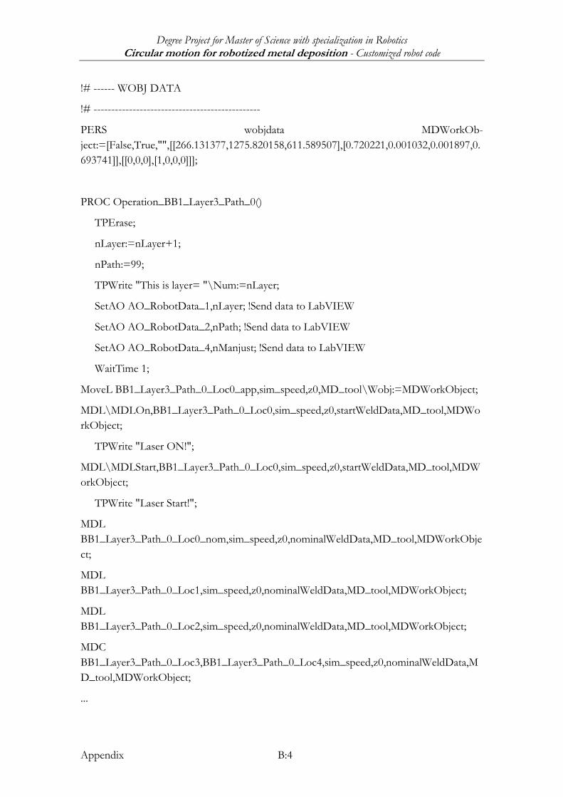
Degree Project for Master of Science with specialization in Robotics Circular motion for robotized metal deposition - Customized robot code
Appendix B:4
!# ------ WOBJ DATA
!# -----------------------------------------------
PERS wobjdata MDWorkOb-
ject:=[False,True,"",[[266.131377,1275.820158,611.589507],[0.720221,0.001032,0.001897,0.
693741]],[[0,0,0],[1,0,0,0]]];
PROC Operation_BB1_Layer3_Path_0()
TPErase;
nLayer:=nLayer+1;
nPath:=99;
TPWrite "This is layer= "\Num:=nLayer;
SetAO AO_RobotData_1,nLayer; !Send data to LabVIEW
SetAO AO_RobotData_2,nPath; !Send data to LabVIEW
SetAO AO_RobotData_4,nManjust; !Send data to LabVIEW
WaitTime 1;
MoveL BB1_Layer3_Path_0_Loc0_app,sim_speed,z0,MD_tool\Wobj:=MDWorkObject;
MDL\MDLOn,BB1_Layer3_Path_0_Loc0,sim_speed,z0,startWeldData,MD_tool,MDWo
rkObject;
TPWrite "Laser ON!";
MDL\MDLStart,BB1_Layer3_Path_0_Loc0,sim_speed,z0,startWeldData,MD_tool,MDW
orkObject;
TPWrite "Laser Start!";
MDL
BB1_Layer3_Path_0_Loc0_nom,sim_speed,z0,nominalWeldData,MD_tool,MDWorkObje
ct;
MDL
BB1_Layer3_Path_0_Loc1,sim_speed,z0,nominalWeldData,MD_tool,MDWorkObject;
MDL
BB1_Layer3_Path_0_Loc2,sim_speed,z0,nominalWeldData,MD_tool,MDWorkObject;
MDC
BB1_Layer3_Path_0_Loc3,BB1_Layer3_Path_0_Loc4,sim_speed,z0,nominalWeldData,M
D_tool,MDWorkObject;
...

Degree Project for Master of Science with specialization in Robotics Circular motion for robotized metal deposition - Customized robot code
Appendix B:5
MDL\MDLStop,BB1_Layer3_Path_0_Loc27,sim_speed,z0,endWeldData,MD_tool,MDW
orkObject;
TPWrite "Laser STOP!";
MDL\MDLOff,BB1_Layer3_Path_0_Loc27,sim_speed,z0,endWeldData,MD_tool,MDW
orkObject;
TPWrite "Laser Off!";
MoveL BB1_Layer3_Path_0_Loc27_end,sim_speed,z0,MD_tool\Wobj:=MDWorkObject;
TPWrite "Laser OFF!";
nPath:=99;
SetAO AO_RobotData_2,nPath; !Send data to LabView;
CheckCutWire;
ENDPROC
ENDMODULE