The process is restarted only when it can regain its old resources as well as the new ones that it is requesting

Protocol # 2

If some requested resources are not available, check whether they are allocated to a process that is waiting for additional resources. If so, preempt these resources from the waiting process and allocate them to the requesting one

This protocol is often applied to resources whose state can be easily saved and restored later, like CPU registers

Circular Wait

Protocol # 1

Impose a total ordering of all resource types, and require that each process requests resources in an increasing order

Protocol # 2

Require that whenever a process requests an instance of a resource type, it has released resources with a lower no

Deadlock Avoidance

The OS is given in advance additional info concerning which resources a process will request & use during its lifetime

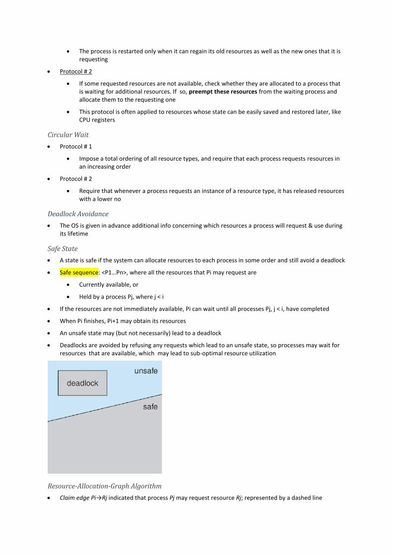
Safe State

A state is safe if the system can allocate resources to each process in some order and still avoid a deadlock

Safe sequence: <P1…Pn>, where all the resources that Pi may request are

Currently available, or

Held by a process Pj, where j < i

If the resources are not immediately available, Pi can wait until all processes Pj, j < i, have completed

When Pi finishes, Pi+1 may obtain its resources

An unsafe state may (but not necessarily) lead to a deadlock

Deadlocks are avoided by refusing any requests which lead to an unsafe state, so processes may wait for resources that are available, which may lead to sub-optimal resource utilization

Resource-Allocation-Graph Algorithm

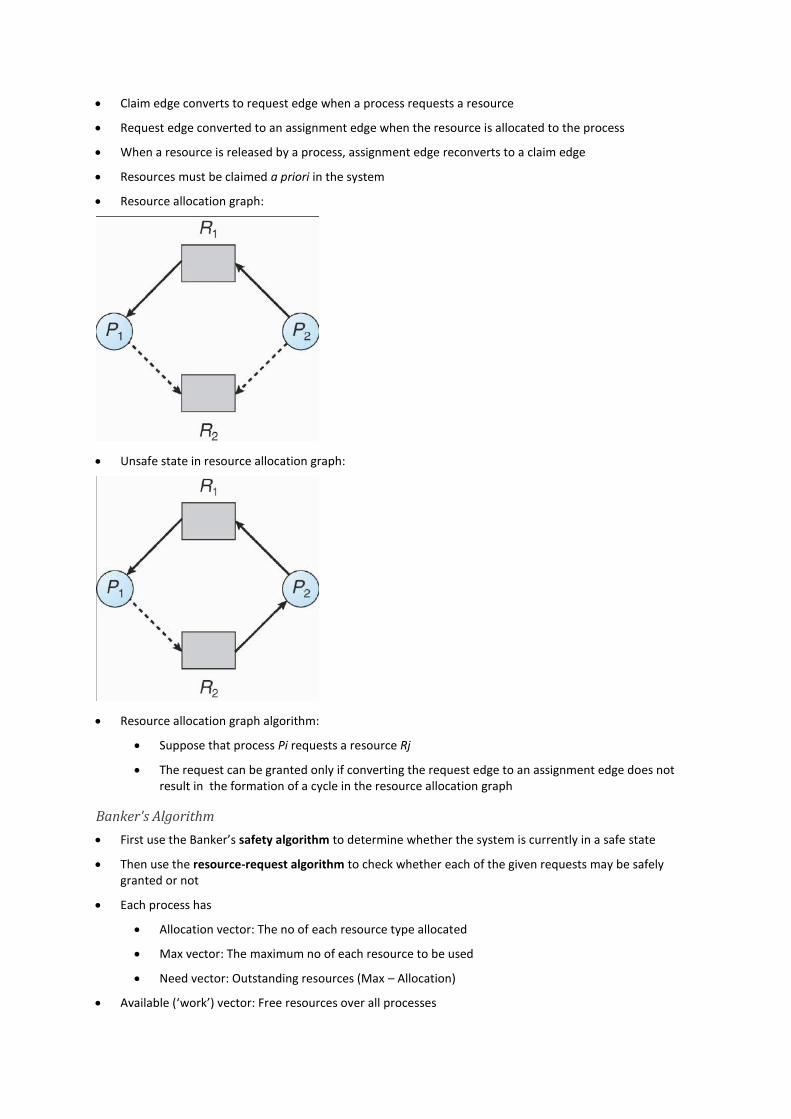
Claim edge Pi→Rj indicated that process Pj may request resource Rj; represented by a dashed line

Claim edge converts to request edge when a process requests a resource

Request edge converted to an assignment edge when the resource is allocated to the process

When a resource is released by a process, assignment edge reconverts to a claim edge

Resources must be claimed a priori in the system

Resource allocation graph:

Unsafe state in resource allocation graph:

Resource allocation graph algorithm:

Suppose that process Pi requests a resource Rj

The request can be granted only if converting the request edge to an assignment edge does not result in the formation of a cycle in the resource allocation graph

Banker's Algorithm

First use the Banker’s safety algorithm to determine whether the system is currently in a safe state

Then use the resource-request algorithm to check whether each of the given requests may be safely granted or not

Each process has

Allocation vector: The no of each resource type allocated

Max vector: The maximum no of each resource to be used

Need vector: Outstanding resources (Max – Allocation)

Available (‘work’) vector: Free resources over all processes

Maximum resource vector: Allocation vectors + Available vector

Finish vector: Indicates which processes are still running

Step 1: Initialize the Finish vector to 0 (0 = false)

Step 2: Search the array Need from the top to find a process needing fewer resources than those Available

Step 3: Assume the process completes, and free its resources:

Add the resources to the Available vector

Subtract the resources from the Process’ Allocation vector

Place 1 in the appropriate place in the Finish vector

Continue until Finish contains only 1s

Problems with the Banker’s algorithm:

It requires a fixed number of resources to allocate

Resources may suddenly break down

Processes rarely know their max resource needs in advance

It requires a fixed number of processes

The no of processes varies dynamically (users log in & out)

Safety Algorithm

Let Work and Finish be vectors of length m and n, respectively. Initialize: (1)

Work = Available

Finish [i] =false fori= 0, 1, …, n-1.

Find and i such that both: (2)

(a) Finish[i] = false

(b) Needi≤Work

If no such i exists, go to step 4.

Work= Work + Allocationi (3)

Finish[i] =true

go to step 2

If Finish[i] == true for all i, then the system is in a safe state (4)

Resource-Request Algorithm

Request= request vector for process Pi. If Requesti[j] = k then process Pi wants k instances of resource type Rj.

If Requesti ≤Needi go to step 2. Otherwise, raise error condition, since process has exceeded its maximum claim (1)

If Requesti≤Available, go to step 3. Otherwise Pimust wait, since resources are not available (2)

Pretend to allocate requested resources to Piby modifying the state as follows: (3)

Available= Available -Request;

Allocationi= Allocationi+ Requesti;

Needi=Needi-Requesti;

If safe ⇒ the resources are allocated to Pi

If unsafe ⇒ Pi must wait, and the old resource-allocation state is restored

An Illustrative Example

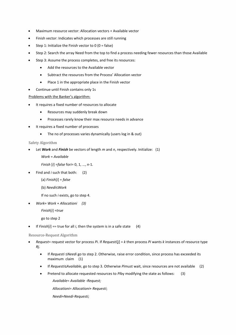
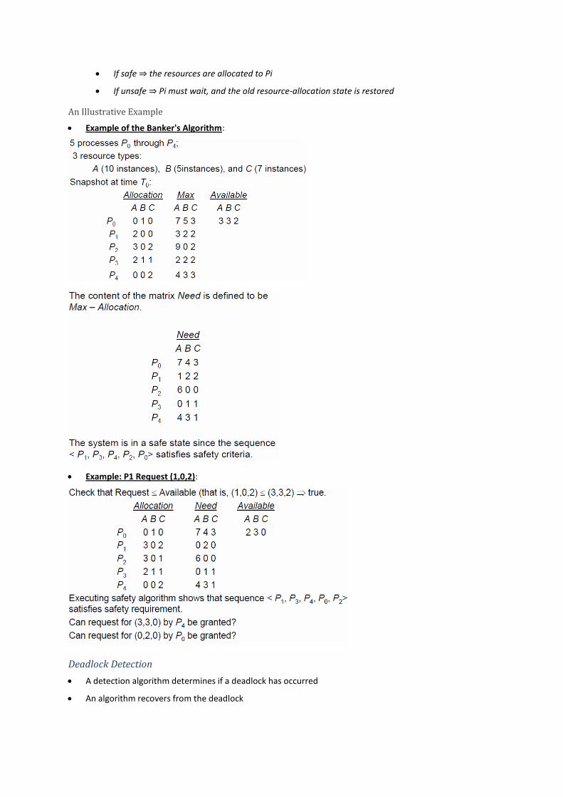
Example of the Banker's Algorithm:

Example: P1 Request (1,0,2):

Deadlock Detection

A detection algorithm determines if a deadlock has occurred

An algorithm recovers from the deadlock

Advantage:

1. Processes don't need to indicate their needs beforehand

Disadvantages:

1. Detection-and-recovery schemes require overhead

2. Potential losses inherent in recovering from a deadlock

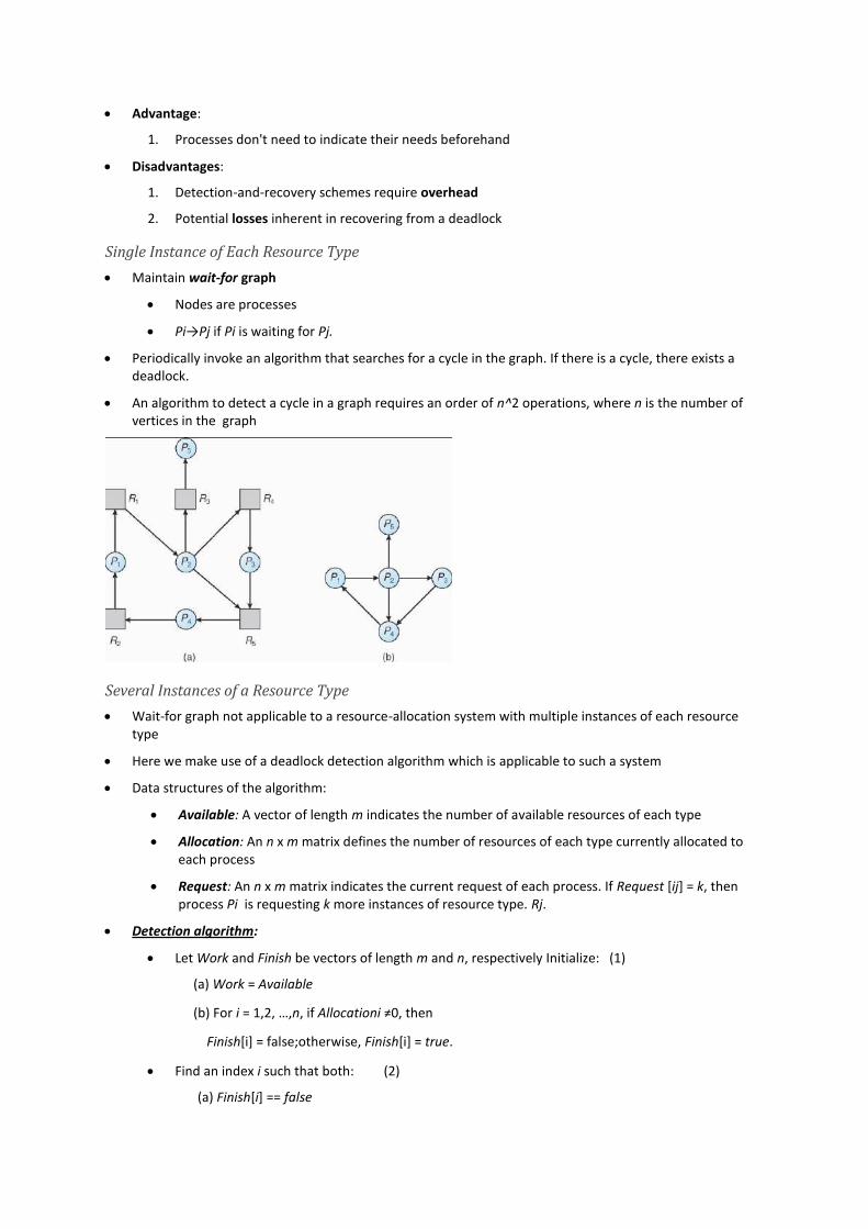
Single Instance of Each Resource Type

Maintain wait-for graph

Nodes are processes

Pi→Pj if Pi is waiting for Pj.

Periodically invoke an algorithm that searches for a cycle in the graph. If there is a cycle, there exists a deadlock.

An algorithm to detect a cycle in a graph requires an order of n^2 operations, where n is the number of vertices in the graph

Several Instances of a Resource Type

Wait-for graph not applicable to a resource-allocation system with multiple instances of each resource type

Here we make use of a deadlock detection algorithm which is applicable to such a system

Data structures of the algorithm:

Available: A vector of length m indicates the number of available resources of each type

Allocation: An n x m matrix defines the number of resources of each type currently allocated to each process

Request: An n x m matrix indicates the current request of each process. If Request [ij] = k, then process Pi is requesting k more instances of resource type. Rj.

Detection algorithm:

Let Work and Finish be vectors of length m and n, respectively Initialize: (1)

(a) Work = Available

(b) For i = 1,2, …,n, if Allocationi ≠0, then

Finish[i] = false;otherwise, Finish[i] = true.

Find an index i such that both: (2)

(a) Finish[i] == false

(b) Requesti ≤Work

If no such i exists, go to step 4

Work = Work + Allocationi (3)

Finish[i] = true

go to step 2.

If Finish[i] == false, for some i, 1 ≤i≤n, then the system is in deadlock state. Moreover, if Finish[i] == false, then Pi is deadlocked (4)

Detection-Algorithm Usage

The frequency of invoking the detection algorithm depends on:

How often a deadlock is likely to occur?

How many processes will be affected by deadlock when it happens?

If detection algorithm is invoked arbitrarily, there may be many cycles in the resource graph and so we would not be able to tell which of the many deadlocked processes "caused" the deadlock

Every invocation of the algorithm adds to computation overhead

Recovery from Deadlock

When a detection algorithm determines that a deadlock exists,

The operator can deal with the deadlock manually

The system can recover from the deadlock automatically

Process Termination

Abort all deadlocked processes

Abort one process at a time until the deadlock cycle is eliminated

In which order should we choose to abort?

Priority of the process

How long process has computed, and how much longer to completion

Resources the process has used

Resources process needs to complete

How many processes will need to be terminated

Is process interactive or batch?

Resource Preemption

Selecting a victim:

We must determine the order of preemption to minimize cost

Cost factors: no. of resources being held, time consumed…

Rollback:

If we preempt a resource from a process, the process can’t go on with normal execution because its missing a resource

We must roll back the process to a safe state & restart it

Starvation:

In a system where victim selection is based primarily on cost factors, the same process may always be picked

To ensure a process can be picked only a small number of times, include the number of rollbacks in the cost factor

Summary

Memory Management

For a program to be executed, it must be mapped to absolute addresses and loaded into memory

As the program executes, it accesses program instructions and data from memory by generating these absolute addresses

Eventually the program terminates and its memory space is declared available so the next program can be loaded & executed

To improve CPU utilization, keep several programs in memory

Selection of a memory-management scheme depends on many factors, especially the hardware design of the system

The OS is responsible for these memory-management activities:

Keeping track of which parts of memory are currently being used and by whom

Deciding which processes are to be loaded into memory when memory space becomes available

Allocating and de-allocating memory space as needed

PART FOUR: MEMORY MANAGEMENT

Chapter 8: Memory-Management Strategies

Chapter Objectives:

To provide a detailed description of various ways of organizing memory hardware

To discuss various memory-management techniques, including paging and segmentation

To provide a detailed description of the Intel Pentium, which supports both pure segmentation and segmentation with paging

Background

The strategies in this chapter have all the same goal:

To keep many processes in memory simultaneously to allow multiprogramming

However, they require that an entire process be in memory before it can execute

Basic Hardware

Program must be brought (from disk) into memory and placed within a process for it to be run

Main memory and registers are only storage CPU can access directly

Register access in one CPU clock (or less)

Main memory can take many cycles

Cache sits between main memory and CPU registers

Protection of memory required to ensure correct operation

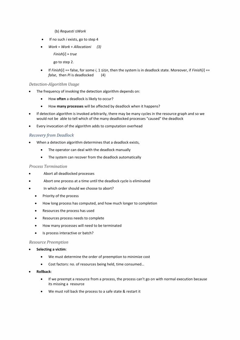
A pair of base and limit registers define the logical (virtual) address space

420940 - 300040 = 120900 (logical address space)

Address Binding

Input queue = the collection of processes on the disk that is waiting to be brought into memory for execution

Processes can normally reside in any part of the physical memory

Addresses in the source program are generally symbolic (‘count’)

A compiler binds these symbolic addresses to relocatable addresses (’14 bytes from the beginning of this module’)

The linkage editor / loader binds these relocatable addresses to absolute addresses (‘74014’)

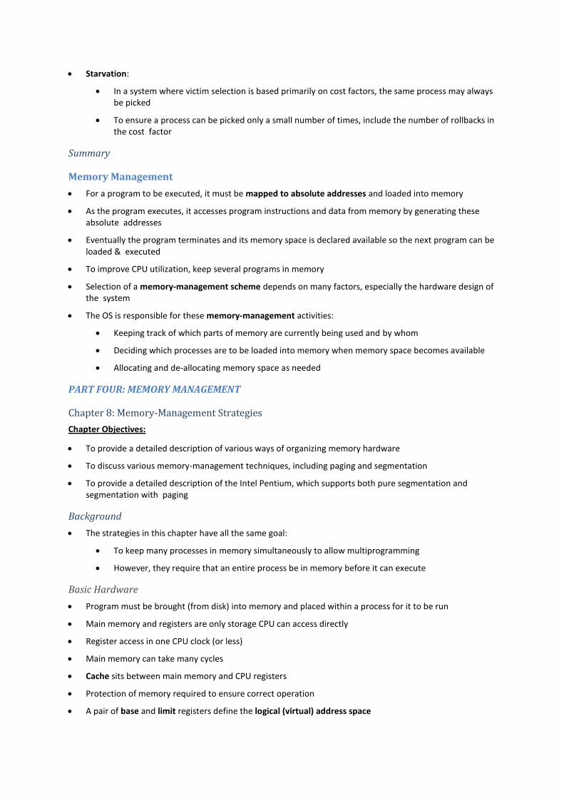
Address binding of instructions and data to memory addresses can happen at three different stages

Compile time:

If memory location known a priori, absolute code can be generated

Must recompile code if starting location changes

Load time:

Must generate relocatable code if memory location is not known at compile time

Execution time:

Binding delayed until run time if the process can be moved during its execution from one memory segment to another

Need hardware support for address maps (e.g., base and limit registers)

Steps a user program needs to go through (some optional) before being executed:

Logical versus Physical Address Space

Logical address = one generated by the CPU

Physical address = one seen by the memory unit, and loaded into the memory-address register of the memory

The compile-time and load-time address-binding methods generate identical logical & physical addresses

The execution-time address-binding scheme results in differing logical (= ‘virtual’) & physical addresses

Logical(virtual)-address space = the set of all logical addresses generated by a program

Physical-address space = the set of all physical addresses corresponding to these logical addresses

Memory-management unit (MMU) = a hardware device that does the run-time mapping from virtual to physical addresses

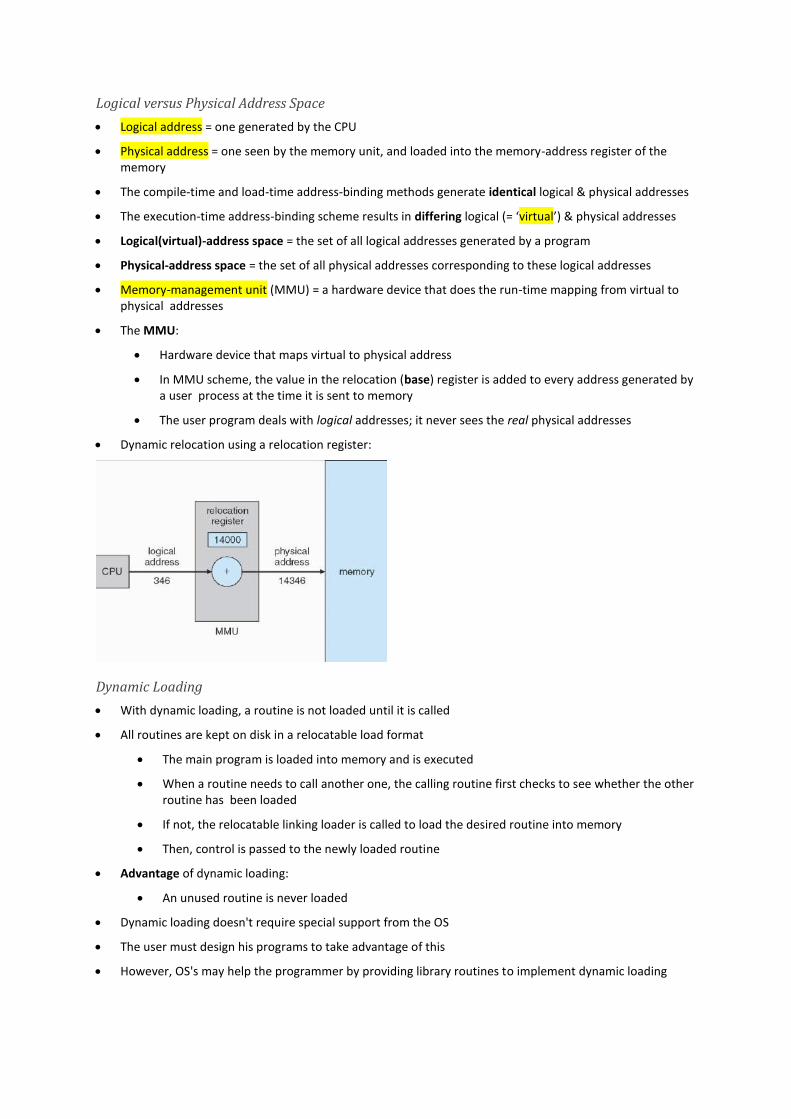
The MMU:

Hardware device that maps virtual to physical address

In MMU scheme, the value in the relocation (base) register is added to every address generated by a user process at the time it is sent to memory

The user program deals with logical addresses; it never sees the real physical addresses

Dynamic relocation using a relocation register:

Dynamic Loading

With dynamic loading, a routine is not loaded until it is called

All routines are kept on disk in a relocatable load format

The main program is loaded into memory and is executed

When a routine needs to call another one, the calling routine first checks to see whether the other routine has been loaded

If not, the relocatable linking loader is called to load the desired routine into memory

Then, control is passed to the newly loaded routine

Advantage of dynamic loading:

An unused routine is never loaded

Dynamic loading doesn't require special support from the OS

The user must design his programs to take advantage of this

However, OS's may help the programmer by providing library routines to implement dynamic loading

Dynamic Linking and Shared Libraries

Static linking:

System language libraries are treated like any other object module and are combined by the loader into the binary program image

Dynamic linking:

Linking is postponed until execution time

Look at image in address binding!!! Also shows dynamic linking

A stub is found in the image for each library-routine reference

Stub:

Code that indicates how to locate the memory-resident library routine, or how to load the library if the routine is not already in memory

Either way, the stub replaces itself with the address of the routine, and executes the routine

The next time that code segment is reached, the library routine is executed directly, with no cost for dynamic linking

Under this scheme, all processes that use a language library execute only one copy of the library code

Unlike dynamic loading, dynamic linking requires help from the OS:

If the processes in memory are protected from one another, then the OS is the only entity that can check to see whether the needed routine is in another process’ memory space

Shared libraries:

A library may be replaced by a new version, and all programs that reference the library will automatically use the new one

Version info is included in both program & library so that programs won't accidentally execute incompatible versions

Swapping

p.322 - 324 TB

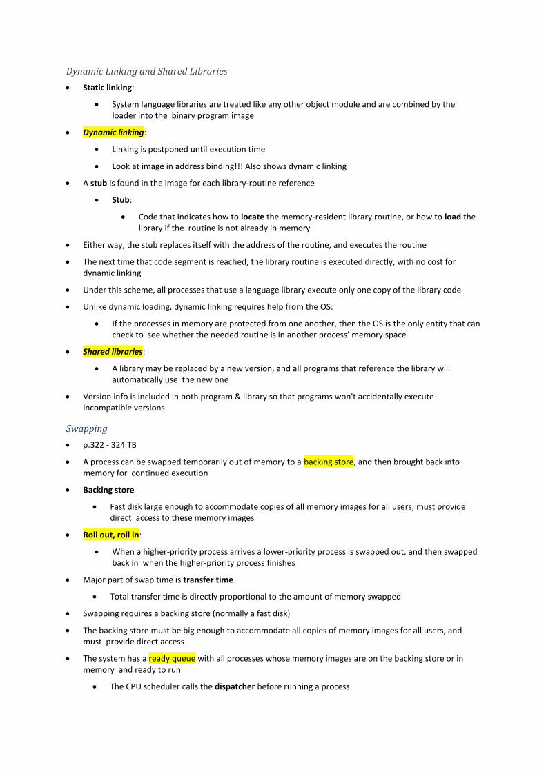
A process can be swapped temporarily out of memory to a backing store, and then brought back into memory for continued execution

Backing store

Fast disk large enough to accommodate copies of all memory images for all users; must provide direct access to these memory images

Roll out, roll in:

When a higher-priority process arrives a lower-priority process is swapped out, and then swapped back in when the higher-priority process finishes

Major part of swap time is transfer time

Total transfer time is directly proportional to the amount of memory swapped

Swapping requires a backing store (normally a fast disk)

The backing store must be big enough to accommodate all copies of memory images for all users, and must provide direct access

The system has a ready queue with all processes whose memory images are on the backing store or in memory and ready to run

The CPU scheduler calls the dispatcher before running a process

The dispatcher checks if the next process in queue is in memory

If not, and there is no free memory region, the dispatcher swaps out a process currently in memory and swaps in the desired one

It then reloads registers and transfers control to the process

The context-switch time in such a swapping system is fairly high

If we want to swap a process, it must be completely idle

Schematic view of Swapping:

Contiguous Memory Allocation

Memory is usually divided into two partitions:

One for the resident OS

One for the user processes

The OS is usually placed in low or high memory (Normally low since interrupt vector is in low memory)

Affected by location of the interrupt vector

Contiguous memory allocation:

Each process is contained in a single contiguous section of memory

Memory Mapping and Protection

The OS must be protected from user processes, and user processes must be protected from one another

Use a relocation register with a limit register for protection

Relocation register contains the smallest physical address

The limit register contains the range of logical addresses

The memory-management unit (MMU) maps the logical address dynamically by adding the value in the relocation register

This mapped address is sent to memory

When the CPU scheduler selects a process for execution, the dispatcher loads the relocation & limit registers

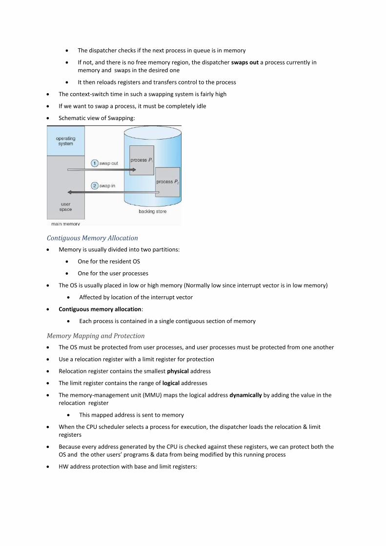
Because every address generated by the CPU is checked against these registers, we can protect both the OS and the other users’ programs & data from being modified by this running process

HW address protection with base and limit registers:

The relocation-register scheme provides an effective way to allow the OS size to change dynamically

Transient OS code:

Code that comes & goes as needed to save memory space and overhead for unnecessary swapping

Memory Allocation

A simple method: divide memory into fixed-sized partitions

Each partition may contain exactly one process

The degree of multiprogramming is bound by the no of partitions

When a partition is free, a process is selected from the input queue and is loaded into the free partition

When the process terminates the partition becomes available

(The above method is no longer in use)

Another method: the OS keeps a table indicating which parts of memory are available and which are occupied

Initially, all memory is available, and is considered as one large block of available memory, a hole

When a process arrives, we search for a hole large enough

If we find one, we allocate only as much memory as is needed

As processes enter the system, they are put into an input queue

When a process is allocated space, it is loaded into memory and can then compete for the CPU

When a process terminates, it releases its memory

We have a list of available block sizes and the input queue

The OS can order the input queue with a scheduling algorithm

Memory is allocated to processes until, finally, there isn't a hole (block of memory) large enough to hold the next process

The OS can then wait until a large enough block is available, or it can skip down the input queue to see whether the smaller memory requirements of some other process can be met

In general, a set of holes of various sizes is scattered throughout memory at any given time

When a process arrives and needs memory, the system searches this set for a hole that is large enough for this process

If the hole is too large, it is split up:

One part is allocated to the process, and the other is returned to the set of holes

On process termination, the memory block returns to the hole set

Adjacent holes are merged to form one larger hole

Solutions to the dynamic storage allocation problem:

First fit (Better and faster)

Allocate the first hole that is big enough

Best fit (Ok)

Allocate the smallest hole that is big enough

Worst fit (Not as good as the other two)

Allocate the largest hole

These algorithms suffer from external fragmentation:

Free memory space is broken into pieces as processes are loaded and removed

Fragmentation

External fragmentation:

Exists when enough total memory space exists to satisfy a request, but it is not contiguous

Internal fragmentation:

Allocated memory may be slightly larger than requested memory; this size difference is memory internal to a partition, but not being used

Compaction is a solution to the problem of external fragmentation

Free memory is shuffled together into one large block

Compaction is not always possible: if relocation is static and is done at assembly / load time, compaction cannot be done

Simplest compaction algorithm:

Move all processes towards one end of memory, leaving one large hole of free memory (Expensive, lots of overhead)

Another solution:

Permit the logical-address space of a process to be noncontiguous

Paging and segmentation allows this solution

Paging

Permits the physical-address space of a process be noncontiguous

Traditionally: support for paging has been handled by hardware

Recent designs: the hardware & OS are closely integrated

Basic Method

Physical memory is broken into fixed-sized blocks called frames

Logical memory is broken into same-sized blocks called pages

When a process is to be executed, its pages are loaded into any available memory frames from the backing store

The backing store has blocks the same size as the memory frames

Every address generated by the CPU is divided into 2 parts:

a page number (to index the page table)

a page offset

The page table contains the base address of each page in memory

This base address is combined with the page offset to define the physical memory address that is sent to the memory unit

The page size, defined by the hardware, is usually a power of 2

Paging schemes have no external, but some internal fragmentation

Small page sizes mean less internal fragmentation

However, there is less overhead involved as page size increases

Also, disk I/O is more efficient with larger data transfers

When a process arrives in the system to be executed, its size, expressed in pages, is examined

(Noncontiguous) frames are allocated to each page of the process

The frame table contains entries for each physical page frame, indicating which are allocated to which pages of which processes

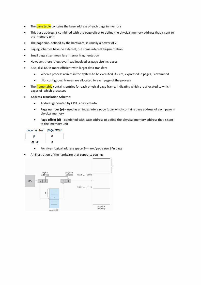
Address Translation Scheme:

Address generated by CPU is divided into:

Page number (p) – used as an index into a page table which contains base address of each page in physical memory

Page offset (d) – combined with base address to define the physical memory address that is sent to the memory unit

For given logical address space 2^m and page size 2^n page

An illustration of the hardware that supports paging:

The paging model of logical and physical memory:

Paging Example: 32-bytee memory and 4-byte pages (p.330)

With the arrival of new processes the following happens:

a) Before allocation

b) After allocation

Hardware Support

Most OS's store a page table for each process

A pointer to the page table is stored in the PCB

Different ways for hardware implementation of the page table:

The page table is implemented as a set of dedicated registers

The CPU dispatcher reloads these registers just like the others

Instructions to load / modify the page-table registers are privileged, so that only the OS can change the memory map

Disadvantage: works only if the page table is reasonably small

The page table is kept in memory, and a page-table base register (PTBR) points to the page table

Changing page tables requires changing only this one register, substantially reducing context-switch time

Disadvantage: two memory accesses are needed to access one byte

Use a small, fast-lookup hardware cache: the translation look-aside buffer (TLB)

The TLB is associative, high-speed memory

Each entry in the TLB consists of a key and a value

When the associative memory is presented with an item, it is compared with all keys simultaneously

If the item is found, the corresponding value field is returned

The search is fast, but the hardware is expensive

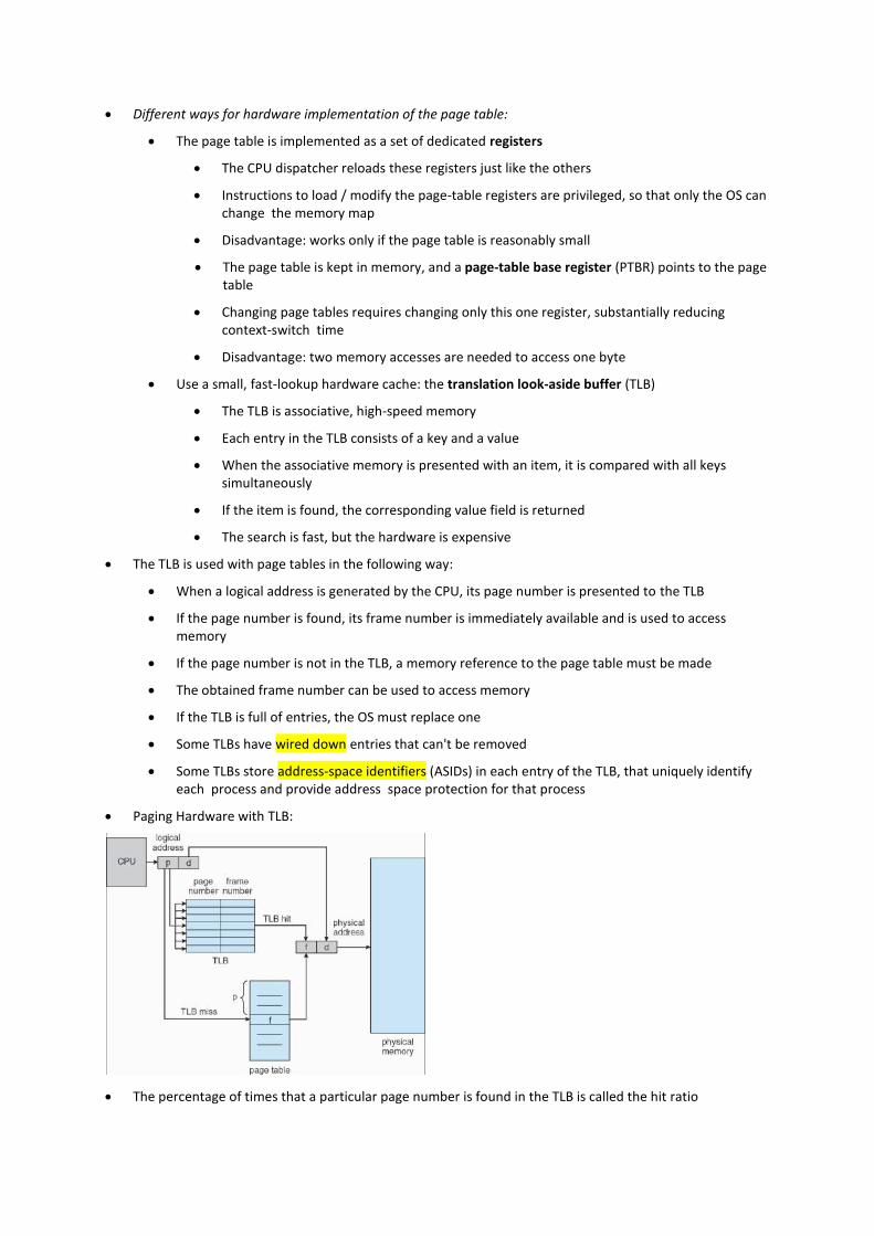
The TLB is used with page tables in the following way:

When a logical address is generated by the CPU, its page number is presented to the TLB

If the page number is found, its frame number is immediately available and is used to access memory

If the page number is not in the TLB, a memory reference to the page table must be made

The obtained frame number can be used to access memory

If the TLB is full of entries, the OS must replace one

Some TLBs have wired down entries that can't be removed

Some TLBs store address-space identifiers (ASIDs) in each entry of the TLB, that uniquely identify each process and provide address space protection for that process

Paging Hardware with TLB:

The percentage of times that a particular page number is found in the TLB is called the hit ratio

Effective access time:

Associative Lookup = ε time unit

Assume memory cycle time is 1 microsecond

Hit ratio –percentage of times that a page number is found in the associative registers; ratio related to number of associative registers

Hit ratio = ±

Effective Access Time(EAT)

EAT = (1 + ε) α+ (2 + ε)(1 –α)

= 2 + ε–α

Protection

Memory protection is achieved by protection bits for each frame

Normally, these bits are kept in the page table

One bit can define a page to be read-write or read-only

Every reference to memory goes through the page table to find the correct frame number, so the protection bits can be checked

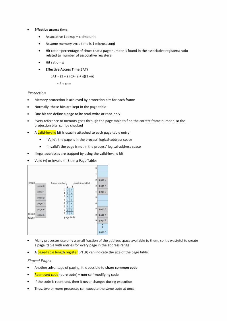
A valid-invalid bit is usually attached to each page table entry

‘Valid’: the page is in the process’ logical-address space

‘Invalid’: the page is not in the process’ logical-address space

Illegal addresses are trapped by using the valid-invalid bit

Valid (v) or Invalid (i) Bit in a Page Table:

Many processes use only a small fraction of the address space available to them, so it’s wasteful to create a page table with entries for every page in the address range

A page-table length register (PTLR) can indicate the size of the page table

Shared Pages

Another advantage of paging: it is possible to share common code

Reentrant code (pure code) = non-self-modifying code

If the code is reentrant, then it never changes during execution

Thus, two or more processes can execute the same code at once

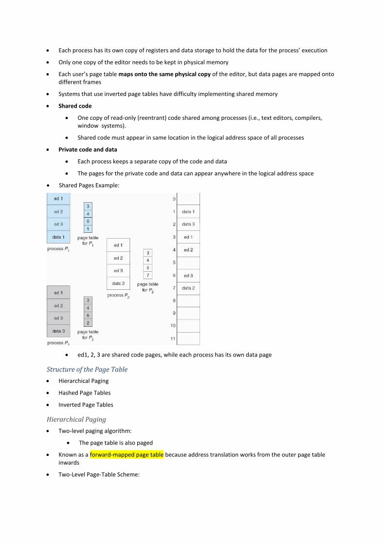
Each process has its own copy of registers and data storage to hold the data for the process’ execution

Only one copy of the editor needs to be kept in physical memory

Each user’s page table maps onto the same physical copy of the editor, but data pages are mapped onto different frames

Systems that use inverted page tables have difficulty implementing shared memory

Shared code

One copy of read-only (reentrant) code shared among processes (i.e., text editors, compilers, window systems).

Shared code must appear in same location in the logical address space of all processes

Private code and data

Each process keeps a separate copy of the code and data

The pages for the private code and data can appear anywhere in the logical address space

Shared Pages Example:

ed1, 2, 3 are shared code pages, while each process has its own data page

Structure of the Page Table

Hierarchical Paging

Hashed Page Tables

Inverted Page Tables

Hierarchical Paging

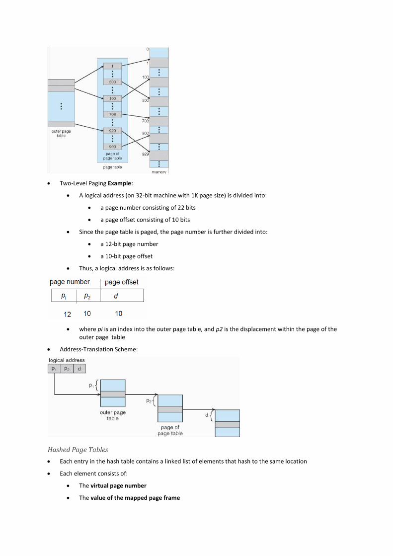
Two-level paging algorithm:

The page table is also paged

Known as a forward-mapped page table because address translation works from the outer page table inwards

Two-Level Page-Table Scheme:

Two-Level Paging Example:

A logical address (on 32-bit machine with 1K page size) is divided into:

a page number consisting of 22 bits

a page offset consisting of 10 bits

Since the page table is paged, the page number is further divided into:

a 12-bit page number

a 10-bit page offset

Thus, a logical address is as follows:

where pi is an index into the outer page table, and p2 is the displacement within the page of the outer page table

Address-Translation Scheme:

Hashed Page Tables

Each entry in the hash table contains a linked list of elements that hash to the same location

Each element consists of:

The virtual page number

The value of the mapped page frame

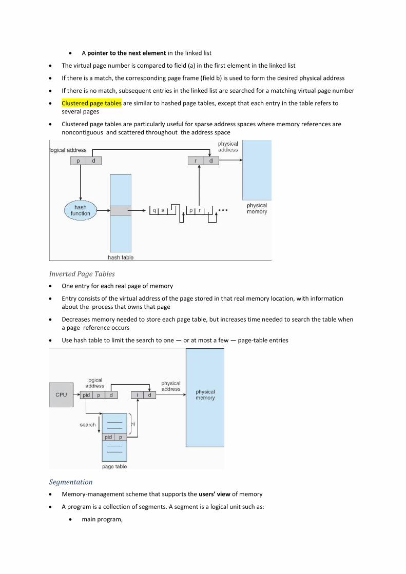
A pointer to the next element in the linked list

The virtual page number is compared to field (a) in the first element in the linked list

If there is a match, the corresponding page frame (field b) is used to form the desired physical address

If there is no match, subsequent entries in the linked list are searched for a matching virtual page number

Clustered page tables are similar to hashed page tables, except that each entry in the table refers to several pages

Clustered page tables are particularly useful for sparse address spaces where memory references are noncontiguous and scattered throughout the address space

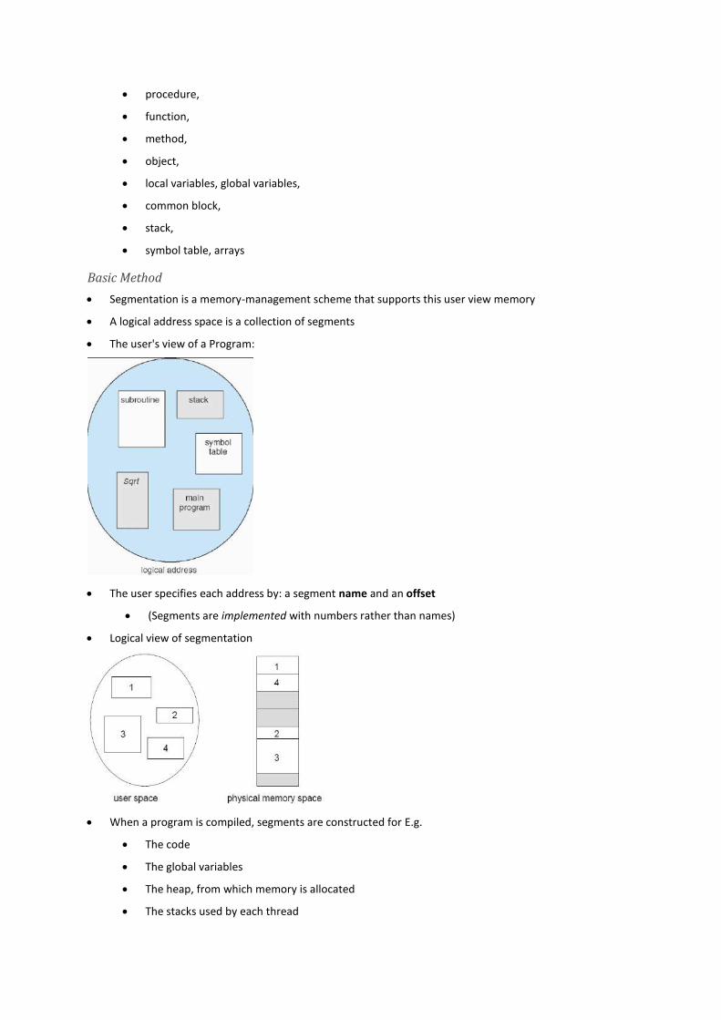
Inverted Page Tables

One entry for each real page of memory

Entry consists of the virtual address of the page stored in that real memory location, with information about the process that owns that page

Decreases memory needed to store each page table, but increases time needed to search the table when a page reference occurs

Use hash table to limit the search to one — or at most a few — page-table entries

Segmentation

Memory-management scheme that supports the users’ view of memory

A program is a collection of segments. A segment is a logical unit such as:

main program,

procedure,

function,

method,

object,

local variables, global variables,

common block,

stack,

symbol table, arrays

Basic Method

Segmentation is a memory-management scheme that supports this user view memory

A logical address space is a collection of segments

The user's view of a Program:

The user specifies each address by: a segment name and an offset

(Segments are implemented with numbers rather than names)

Logical view of segmentation

When a program is compiled, segments are constructed for E.g.

The code

The global variables

The heap, from which memory is allocated

The stacks used by each thread

The procedure call stack, to store parameters

The code portion of each procedure or function

The local variables of each procedure and function

The loader would take all these segments and assign them segment numbers

Hardware

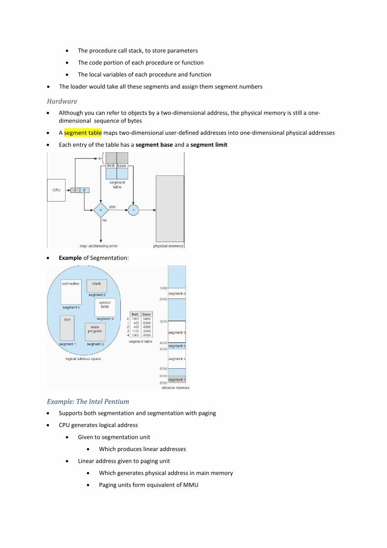
Although you can refer to objects by a two-dimensional address, the physical memory is still a one-dimensional sequence of bytes

A segment table maps two-dimensional user-defined addresses into one-dimensional physical addresses

Each entry of the table has a segment base and a segment limit

Example of Segmentation:

Example: The Intel Pentium

Supports both segmentation and segmentation with paging

CPU generates logical address

Given to segmentation unit

Which produces linear addresses

Linear address given to paging unit

Which generates physical address in main memory

Paging units form equivalent of MMU

Pentium Segmentation

Pentium Paging

Linux on Pentium Systems

Summary

Chapter 9: Virtual-Memory Management

Virtual memory is a technique that allows the execution of processes that are not completely in memory

Objectives:

To describe the benefits of a virtual memory system

To explain the concepts of demand paging, page-replacement algorithms, and allocation of page frames

To discuss the principle of the working-set model

Background

In many cases, the entire program is not needed:

Unusual error conditions are almost never executed

Arrays & lists are often allocated more memory than needed

Certain options & features of a program may be used rarely

Benefits of executing a program that is only partially in memory

More programs could be run at the same time

Programmers could write for a large virtual-address space and need no longer use overlays

Less I/O would be needed to load / swap programs into memory, so each user program would run faster

Virtual memory – separation of user logical memory from physical memory

Only part of the program needs to be in memory for execution

Logical address space can therefore be much larger than physical address space

Allows address spaces to be shared by several processes

Allows for more efficient process creation

Virtual memory can be implemented by:

Demand paging

Demand segmentation

Diagram showing virtual memory that is larger than physical memory:

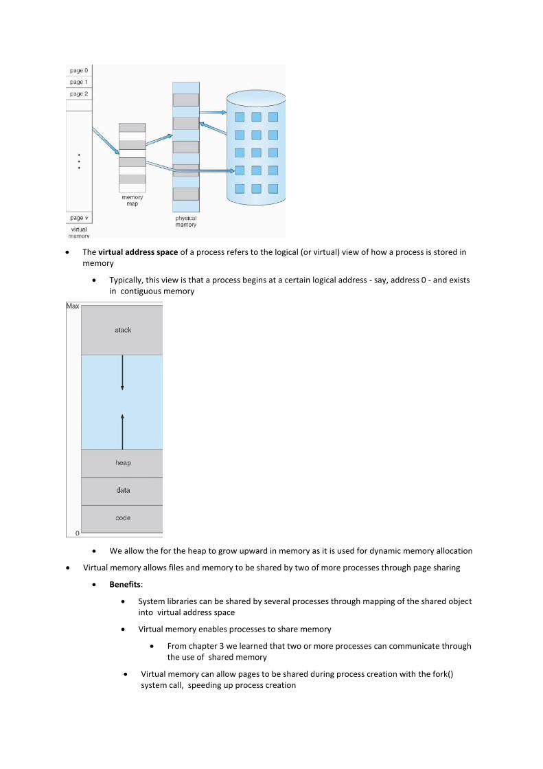
The virtual address space of a process refers to the logical (or virtual) view of how a process is stored in memory

Typically, this view is that a process begins at a certain logical address - say, address 0 - and exists in contiguous memory

We allow the for the heap to grow upward in memory as it is used for dynamic memory allocation

Virtual memory allows files and memory to be shared by two of more processes through page sharing

Benefits:

System libraries can be shared by several processes through mapping of the shared object into virtual address space

Virtual memory enables processes to share memory

From chapter 3 we learned that two or more processes can communicate through the use of shared memory

Virtual memory can allow pages to be shared during process creation with the fork() system call, speeding up process creation

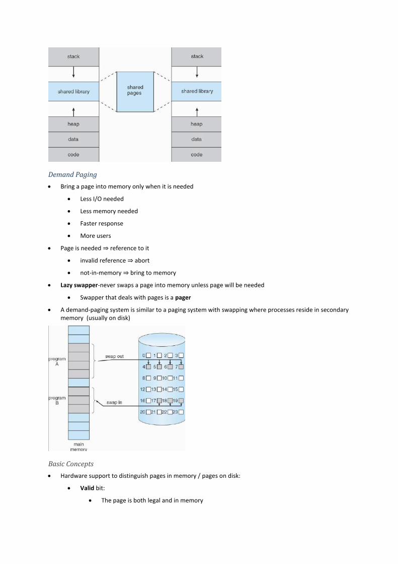
Demand Paging

Bring a page into memory only when it is needed

Less I/O needed

Less memory needed

Faster response

More users

Page is needed ⇒ reference to it

invalid reference ⇒ abort

not-in-memory ⇒ bring to memory

Lazy swapper-never swaps a page into memory unless page will be needed

Swapper that deals with pages is a pager

A demand-paging system is similar to a paging system with swapping where processes reside in secondary memory (usually on disk)

Basic Concepts

Hardware support to distinguish pages in memory / pages on disk:

Valid bit:

The page is both legal and in memory

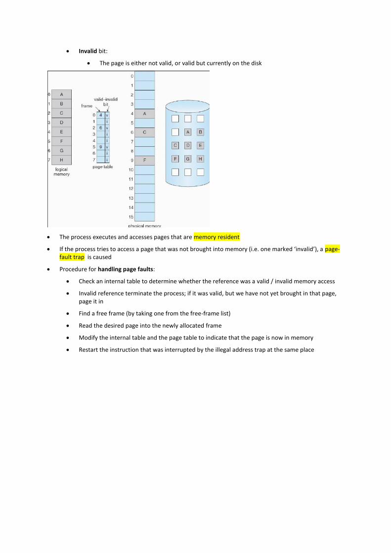
Invalid bit:

The page is either not valid, or valid but currently on the disk

The process executes and accesses pages that are memory resident

If the process tries to access a page that was not brought into memory (i.e. one marked ‘invalid’), a page-fault trap is caused

Procedure for handling page faults:

Check an internal table to determine whether the reference was a valid / invalid memory access

Invalid reference terminate the process; if it was valid, but we have not yet brought in that page, page it in

Find a free frame (by taking one from the free-frame list)

Read the desired page into the newly allocated frame

Modify the internal table and the page table to indicate that the page is now in memory

Restart the instruction that was interrupted by the illegal address trap at the same place

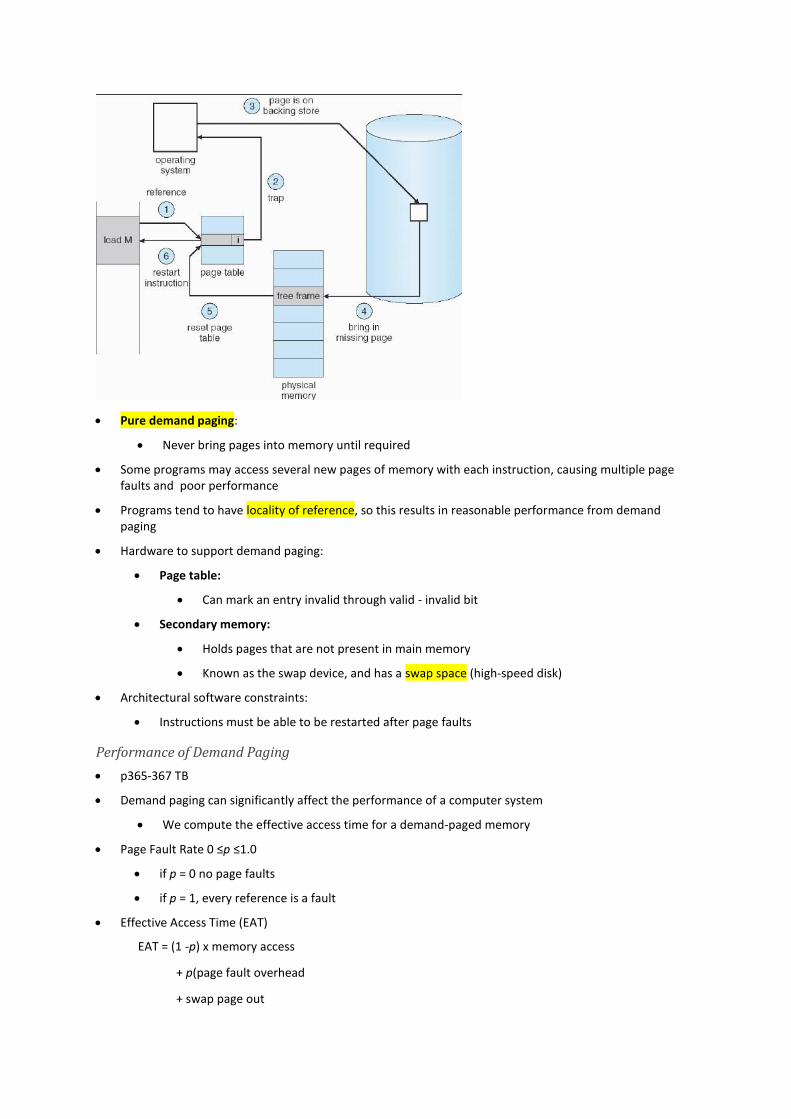
Pure demand paging:

Never bring pages into memory until required

Some programs may access several new pages of memory with each instruction, causing multiple page faults and poor performance

Programs tend to have locality of reference, so this results in reasonable performance from demand paging

Hardware to support demand paging:

Page table:

Can mark an entry invalid through valid - invalid bit

Secondary memory:

Holds pages that are not present in main memory

Known as the swap device, and has a swap space (high-speed disk)

Architectural software constraints:

Instructions must be able to be restarted after page faults

Performance of Demand Paging

p365-367 TB

Demand paging can significantly affect the performance of a computer system

We compute the effective access time for a demand-paged memory

Page Fault Rate 0 ≤p ≤1.0

if p = 0 no page faults

if p = 1, every reference is a fault

Effective Access Time (EAT)

EAT = (1 -p) x memory access

+ p(page fault overhead

+ swap page out