cirrus particle size distribution bimodality derived from
TRANSCRIPT
CIRRUS PARTICLE SIZE DISTRIBUTION BIMODALITY DERIVED FROM
GROUND-BASED RADAR-LIDAR RETRIEVALS
by
Yang Zhao
A thesis submitted to the faculty of The University of Utah
in partial fulfillment of the requirements for the degree of
Master of Science
Department of Atmospheric Sciences
The University of Utah
May 2011

Copyright © Yang Zhao 2011
All Rights Reserved

T h e U n i v e r s i t y o f U t a h G r a d u a t e S c h o o l
STATEMENT OF THESIS APPROVAL
The thesis of
has been approved by the following supervisory committee members:
, Chair Date Approved
, Member
Date Approved
, Member
Date Approved
and by , Chair of
the Department of
and by Charles A. Wight, Dean of The Graduate School.

ABSTRACT
To better understand the role of small particles in the microphysical processes and the
radiative properties of cirrus, the reliability of the historical in situ measurement database
must be understood. A means of establishing this validity is to assume that the in situ
measurements are at least consistent, in a broad sense, with the remote sensing data, and
vice versa. In this study, an algorithm using Doppler radar moments and Raman lidar
extinction is developed to retrieve a bimodal particle size distribution and its uncertainty.
Case studies and statistics compiled over an entire year show that the existence of high
concentrations in excess of 1 cm-3 of small particles in cirrus is not consistent with any
reasonable interpretation of remote sensing data and is therefore likely from an artifact of
the in situ measurement process. This study shows that while the particle concentrations
from the Two-Dimensional Cloud Probe generally agree well with the retrieval results,
simultaneous concentrations from the Forward Scattering Spectrometer Probe are much
higher than the concentrations of small particles implied by the remote sensing
measurements. The one-year statistics of the cirrus microphysical properties, including
the ice water content, the effective radius and the total particle concentration, show that
the occurrence frequency of the concentrations larger than 1 cm-3 is below 1%, and, given
the possibility of errors in retrieved concentration as large as 100%, this study concludes
that the existence of particle concentrations in cirrus in excess of 1 cm-3 is extraordinarily
rare instead of common as suggested by uncritical acceptance of in situ data.

TABLE OF CONTENTS
ABSTRACT ....................................................................................................................... iii
LIST OF FIGURES ........................................................................................................... vi
LIST OF TABLES ............................................................................................................ vii
1. INTRODUCTION .......................................................................................................... 1
1.1Motivation .................................................................................................................. 1 1.2 Data and Method Overview ...................................................................................... 4
2. ALGORITHM DEVELOPMENT .................................................................................. 6
2.1 Particle Size Distribution Assumption ...................................................................... 6 2.2 Forward Model.......................................................................................................... 7
2.2.1 Radar Reflectivity ............................................................................................... 8 2.2.2 Doppler Velocity .............................................................................................. 10 2.2.3 Optical Extinction ............................................................................................. 11 2.2.4 Parameter Reduction and the Fourth Forward Model Equation ....................... 12 2.2.5 Expressions for the Microphysical Properties .................................................. 14
2.3 Retrieval Algorithm Implementation ...................................................................... 15 2.3.1 Optimal Estimation Method ............................................................................. 16 2.3.2 Initial Guess ...................................................................................................... 19 2.3.3 Two Problems in the Implementation .............................................................. 21
2.4 Retrieval Uncertainty Evaluation ............................................................................ 23 2.4.1 Measurement Error ........................................................................................... 25 2.4.2 Power Law Model Parameter Error .................................................................. 26 2.4.3 Retrieval Error Estimation ................................................................................ 28 2.4.4 Sensitivity Test ................................................................................................. 30
3. CASE STUDY .............................................................................................................. 40
3.1 Comparing In Situ Measurements with Ground-Based Retrievals ......................... 40 3.1.1 Difficulties in Comparison ............................................................................... 40 3.1.2 Statistical Method ............................................................................................. 42
3.2 In Situ Measurements ............................................................................................. 45 3.2.1 Particle Images from the CPI ............................................................................ 45 3.2.2 Number Concentration from the 2DC and the FSSP ........................................ 46 3.2.3 Ice Water Content from the CVI ...................................................................... 47
3.3 Case Study on March 9th 2000 ................................................................................ 48 3.3.1 Synopsis and Flight Information ...................................................................... 48
v
3.3.2 Comparison of PSD .......................................................................................... 49 3.3.3 Comparison of IWC.......................................................................................... 51
4. ONE-YEAR STATISTICS ........................................................................................... 65
4.1 PSD Bimodality Statistics ....................................................................................... 66 4.2 PDFs of IWC, Effective Radius and Concentration ............................................... 69
4.2.1 PDF of IWC ...................................................................................................... 69 4.2.2 PDF of Effective Radius ................................................................................... 70 4.2.3 PDF of Concentration ....................................................................................... 71
5. SUMMARY .................................................................................................................. 78
APPENDICES
A. SINGLE MODE RETRIEVAL ALGORITHM .......................................................... 82
B. CONVERSION OF AERODYNAMIC DIAMETER ................................................. 85
REFERENCES ................................................................................................................. 86
LIST OF FIGURES
Figure Page
1. A bimodal particle size distribution with six parameters. ............................................. 34
2. Flowchart of the derivation of the initial guesses. ........................................................ 35
3. Contour of the misfit function....................................................................................... 35
4. PSD retrievals comparison. ........................................................................................... 36
5. Radar backscattering cross section from DDA and empirical relation. ........................ 37
6. Examples of PSD retrieval uncertainty due to empirical relationship. ......................... 38
7. Coordinates of the airplane positions during the first five legs. ................................... 55
8. Flight path and radar reflectivity cross section on March 9th 2000. ............................. 56
9. Comparisons of PSD retrievals and PSD in situ measurements. .................................. 57
10. Comparisons of single mode PSD retrievals with in situ data. ................................... 58
11. PDF of retrievals and in situ data. ............................................................................... 61
12. PSD retrieval and PSD fit with different misfits. ....................................................... 73
13. Bimodality frequency histogram in terms of reflectivity and temperature. ................ 75
14. Bimodality vertical profiles for cirrus with different temperatures. ........................... 75
15. PDF of IWC from retrievals. ...................................................................................... 76
16. PDF of effective radius from retrievals. ..................................................................... 76
17. PDF of concentration from retrievals. ........................................................................ 77
LIST OF TABLES
Table Page
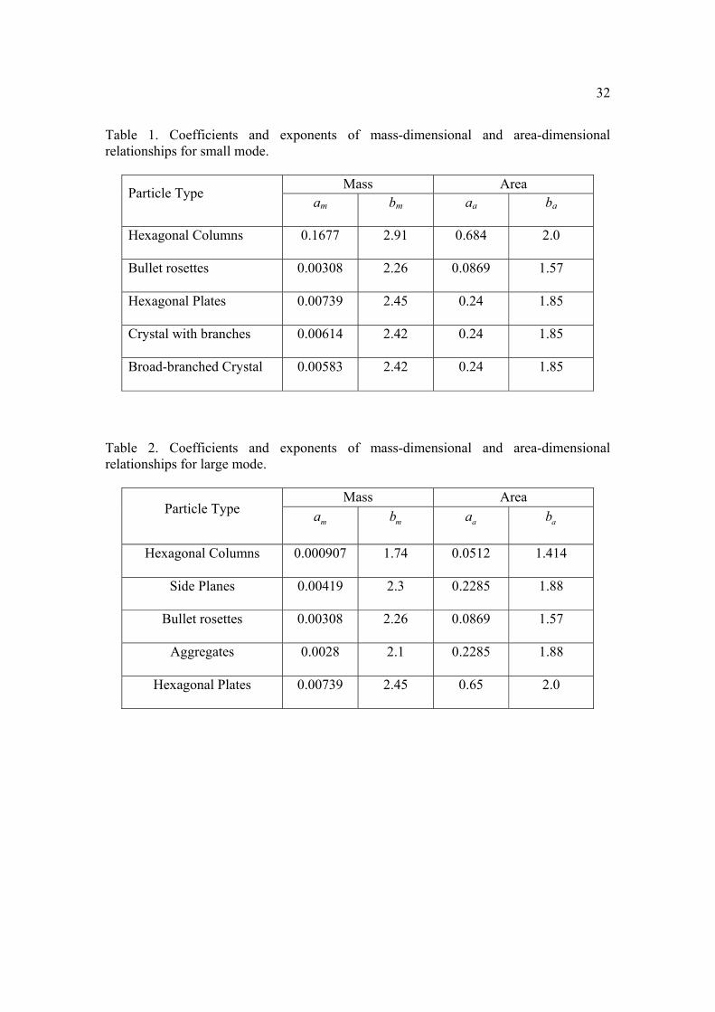
1. Coefficients and exponents of mass-dimensional and area-dimensional relationships for small mode. ......................................................................................................... 32
2. Coefficients and exponents of mass-dimensional and area-dimensional relationships for large mode. .......................................................................................................... 32
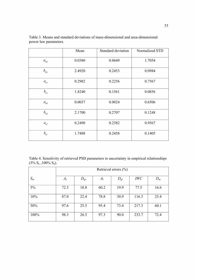
3. Means and standard deviations of mass-dimensional and area-dimensional power law parameters. ................................................................................................................ 33
4. Sensitivity of retrieved PSD parameters to uncertainty in empirical relationships (5% Sε ,100% Sa). ............................................................................................................. 33
5. Sensitivity of retrieved PSD parameters to uncertainty in measurements (5% Sm , 100% Sa). ............................................................................................................................. 34
6. UND Citation Instruments and measurements. ............................................................ 54
7. Percentage of IWC50 in the total IWC. ......................................................................... 54
8. The mean and standard deviation for IWC in situ data and IWC retrieval. .................. 55
CHAPTER 1
INTRODUCTION
1.1 Motivation
Cirrus clouds play an important role in regulating the earth’s energy budget through
their interactions with the solar and terrestrial radiation. However, they remain a poorly
understood component of the climate system (Stephens, 2005). To better represent the
feedback of cirrus on the climate system in global climate models, the processes that
control the evolution of the macrophysical and microphysical properties of cirrus must be
understood as well. This chain of understanding must rest on a foundation of reliable
measurements of microphysical properties, including particle size distributions (PSD) and
integral properties of the PSD such as water content, mean particle size, and total particle
concentration.
At the microphysical level, how light is scattered by ice crystals, especially small ice
crystals, is critically important to the solar radiative properties of cirrus, which have a
large impact on the albedo of the earth. Heymsfield and Platt (1984) found that as much
as 53% of the total visible extinction could be due to small particles in the size range of
1-20 microns. Arnott et al. (1994) showed that small particles could contribute
significantly to and sometimes dominate both the solar extinction and the infrared
emission. So to better quantify the scattering effects of ice crystals, many field
experiments have been conducted and many in situ measurements have been made. For
2
example, based on in situ measurements from the Forward Scattering Spectrometer Probe
(FSSP) and the laser imaging Two-Dimensional Cloud Probe (2DC) from 17 flights in
midlatitude cirrus during the Atmospheric Radiation Measurement (ARM) and First
International Satellite Cloud Climatology Project (ISCCP) Regional Experiment (FIRE)
Intensive Observation Periods (IOP), Ivanova et al. (2001) parameterize cirrus Particle
Size Distribution (PSD) as bimodal, one mode for small particles and the other mode for
large particles. Gayet et al. (2002) show that high concentrations (5 to 10 cm-3) of small
ice crystals are a relatively common microphysical feature of cirrus clouds by using
combined measurements from four different in situ instruments: the Counterflow Virtual
Impactor (CVI), the Polar Nephelometer, the FSSP and the 2DC during the
Interhemispheric Differences in Cirrus Properties From Anthropogenic Emissions (INCA)
field experiment. Based on 22 Learjet missions flown in midlatitude cirrus, Lawson et al.
(2006) conclude that small particles with maximum dimension less than 50 microns
account for 99% of the total number concentrations, 69% of the extinction, and 40% of
the mass in midlatitude cirrus.
However, recent studies also suggest that some in situ measurements, such as
measurements from the FSSP, may be contaminated by ice crystal shattering on probe
inlets, and the particle shattering may have a big effect on the in situ measurements. For
example, Field et al. (2003) show that the ice particle interarrival times measured by a
fast FSSP can be well characterized by a Markov chain model with two independent
Poisson processes, and the debris from ice crystal shattering and the unaffected particles
may be the sources for these two different Poisson processes. Korolev and Isaac (2005)
demonstrate two possible physical mechanisms for the ice crystal shattering: mechanical

3
impact with the probe arms and interaction with the aerodynamic field around the probe
housing. By using data from Optical Array Probes (OAP) 2DC, OAP 2DP and the high
volume precipitation spectrometer, they found that the fraction of shattered ice crystals
may make up more than 10% of the total number of sampled particles for aggregates of
dendrites. Heymsfield (2007) further investigated the shattering effects on measurements
from the Cloud and Aerosol Spectrometer (CAS), the Cloud Integrating Nephelometer
(CIN), as well as the FSSP, and he suggests that shattering adds about 15% to the large
IWC from the FSSP, and the shattering effect on FSSP and CIN measurements is even
more for optical extinction. By using the in situ measurements from the Tropical Warm
Pool International Cloud Experiment (TWP-ICE), McFarquhar et al. (2007) showed that
the number concentrations of particles with 3 < D < 50 microns (D: maximum dimension)
measured by the CAS with an inlet are 91 (with standard deviation of 127) times larger
than those from the Cloud Droplet Probe (CDP), which does not have an inlet, and thus
has no effect from the inlet shattering.
Some researchers recently use satellite retrievals to compare with airborne in situ
measurements, and provide indirect evidence of the particle shattering effect. For
example, Davis et al. (2009) show that the ratio of optical thickness to effective diameter
from the in situ measurements differs from the MODIS value in a manner that is roughly
consistent with previous claims of the particle shattering effect. However, they also claim
that biases in the MODIS retrievals cannot be ruled out.
In this study, to further verify the airborne in situ measurements of small particles in
cirrus, the number concentration measurements from the FSSP will be directly compared
to the ground-based remote sensing retrievals. Measurements from two active remote
4
sensors, millimeter wavelength Doppler radar and Raman lidar, will be used in the
retrieval algorithm, and an inversion technique will provide both the optimal solutions for
retrievals and the retrieval uncertainties.
1.2 Data and Method Overview
The remote sensing measurements used in this study are from the Millimeter
Wavelength Cloud Radar (MMCR) and the Raman lidar at the ARM Southern Great
Plain (SGP) site.
The ARM MMCR radars are zenith-pointing radars that operate at a frequency of
34.86 GHz. The calibration uncertainty for the radar reflectivity is about 1-2 dBZ, and the
uncertainty for the mean Doppler velocity and spectral width is about 0.1 m s-1
(Clothiaux et al., 1999). The MMCR radar data used in this study are the water-
equivalent radar reflectivity factor , and the cloud particle terminal fall velocity ,
which is retrieved from an algorithm described in Deng and Mace 2006 (hereafter DM06).
The ARM Raman lidar is currently operational only at the SGP site, and the lidar data
used in this study are the extinction estimated from the lidar measurements (Goldsmith et
al., 1998). For Raman lidar, the inelastic (Raman) backscatter signal is affected only by
extinction, so the formalism used to estimate the optical extinction does not suffer from
the fact that two physical quantities, the aerosol backscatter and extinction coefficients,
must be determined from only one measured lidar signal, which is the case for lidar
systems built based on elastic scattering (Ansmann et al., 1990). The details of the
formalism to derive extinction from Raman lidar measurements can be found in Ansmann
et al. (1990) and the calculations were performed by Dr. Jennifer Comstock of the Pacific
5
Northwest National Laboratory (Comstock, personal communication, 2007).
In sum, the remote sensing data used in the algorithm are the radar reflectivity factor
from the MMCR, the terminal fall velocity retrieval from the algorithm described in
DM06, and the lidar extinction estimated from Raman lidar measurements.
The approach used to address the question of the concentrations of small particles is
first to assume that the PSD is bimodal, as suggested by the in situ measurements. Then,
since lidar measurements are sensitive to small particles in cirrus while radar
measurements are more sensitive to large particles, lidar and radar measurements are
used to calculate the first guesses of small mode PSD parameters and large mode PSD
parameters, respectively. Specifically, two modified gamma functions are used to
approximate these two modes, and then based on forward model equations from radar
reflectivity, Doppler velocity and lidar extinction. An inversion of the forward model
equations is based on a Maximum A Posteriori (MAP) criterion, and a Gaussian PDF
assumption is used to get both the optimal estimates of the PSD parameters and their
retrieval uncertainties. The PSD retrievals from the remote sensing measurements are
compared with the PSD in situ measurements to test consistency. Finally, the statistics of
the microphysical properties from one year of retrievals is examined to see if the remote
sensing data are consistent with the ubiquitous occurrence of high concentrations of small
particles in cirrus.
The details of the retrieval algorithm are described in Chapter 2, and a case study is
performed in Chapter 3 using the data from the 2000 Cloud IOP. In Chapter 4, long-term
observations at the ARM SGP site are used to give the statistics of cirrus microphysical
properties, and a summary is given in Chapter 5.

CHAPTER 2
ALGORITHM DEVELOPMENT
2.1 Particle Size Distribution Assumption
We allow for the possibility that the particle size distribution (PSD) of a cirrus volume
could have distinct populations of small and large particles that may be entirely unrelated
to one another. This allowance requires a bimodal size distribution assumption in the
retrieval algorithm.
The bimodal size distribution assumption has been used in previous applications such
as in cirrus cloud models (Mitchell, 1996) and also in the parameterization of visible
extinction for ice clouds (Platt et al., 1997). Donovan (2003) was the first to use the
bimodal size distribution assumption in a retrieval algorithm to estimate ice cloud
effective particle size profiles. In his algorithm, two generalized gamma functions with
three parameters fixed to constants are used to represent the particle size distribution.
In the algorithm developed here, two modified gamma functions are used to approximate
the small particle mode and the large particle mode separately, and for each mode the
gamma function has the following form:
( ) ⎟⎟⎠
⎞⎜⎜⎝
⎛ −⎟⎟⎠
⎞⎜⎜⎝
⎛=
xg
xg
xgxx D
DDDDADN
x
,
,
,
expα
(2.1)
7
where subscript x stands for the large particle mode (l) and the small particle mode (s),
D is the particle maximum dimension, ,g xD is the distribution parameter that controls
the slope of the distribution, xA is the number of particles per unit volume per unit
length at the size ,g xD , and xα is the parameter to control the breadth of the distribution.
Subscript l and s are used to stand for the large mode and small mode parameters,
respectively, of the bimodal particle size distribution. So the bimodal PSD N(D) can be
expressed as:
( ) ( ) ( )DNDNDN sl += (2.2)
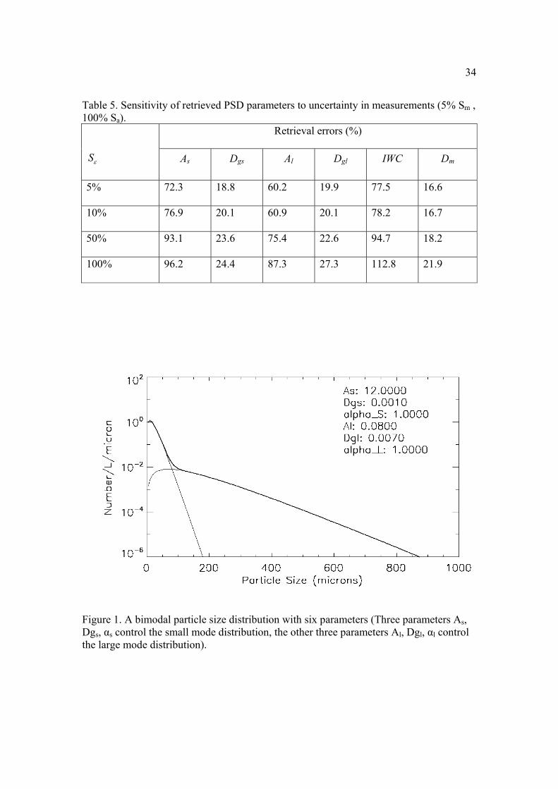
This distribution, in its most general form, has six independent degrees of freedom.
One example distribution is shown in Figure 1.
2.2 Forward Model
The algorithm is formulated in terms of three measurables: the liquid water equivalent
radar reflectivity factor ( ), the Doppler velocity ( ) observed at a wavelength that is
large with respect to D, and the extinction ( ) derived at a wavelength that is small
with respect to D. provides information that is strongly weighted to the largest
particles in N(D), and when a prominent large particle mode is present, can be nearly
entirely determined by it. is determined by the second moment of N(D) and, when a
prominent small mode is present, this quantity can be nearly entirely described by the
small mode PSD. , on the other hand, provides a bridge between the large and small
particle modes since the particle terminal velocity depends on the ratio of the particle
8
mass to cross sectional area (Mitchell, 1996) although the measurement is weighted
by and, therefore, has a similar large particle weighting.
In the following development, the forward model equations describing the measured
quantities are derived in terms of the assumed bimodal particle size distribution. It should
be noted that the derivation of the forward model equations depends on assumptions
regarding the distribution of certain intensive properties such as mass and cross sectional
area as a function of particle maximum dimension. These relationships depend on the
assumed ice crystal habit. The resulting uncertainties due to these assumptions are
discussed in detail.
2.2.1 Radar Reflectivity Since Rayleigh scattering is valid for particles less than 800 microns at 35 GHz
wavelength (Donovan et al., 2004), under the assumption of Rayleigh scattering, and
assuming for the moment that the cloud particles are solid spheres, the radar reflectivity
factor Z can be written as:
6
0
( )Z N D D dD∞
= ∫ (2.3)
However, for cirrus clouds, the ice crystals are not spherical, so it is common practice
to use water-equivalent radar reflectivity factor Ze instead of Z, and it can be expressed as:
6
0
( ) zbe zZ a N D D dD
∞+= ∫ (2.4)
9
where parameters az and bz are power law parameters to fit the radar backscattering cross
section from ice crystals with a certain shape (Aydin et al., 1999).
Following DM06, the power law parameters az and bz can be expressed in terms of the
coefficient am and exponent bm in a mass-dimensional power law relationship
( ) mbmM D a D= as:
2 226i
z mw i
Ka aK πρ
⎛ ⎞= ⎜ ⎟
⎝ ⎠ (2.5)
2 6z mb b= − (2.6)
where ρi is the density of solid ice, Ki is the complex dielectric factor for ice and Kw is the
complex dielectric factor for water.
Substituting Equation (2.2) into Equation (2.4), and integrating over all particle sizes,
Ze can be expressed as a function of size distribution parameters and radar backscattering
cross section parameters az and bz:
( )∑∑=
+
=
++Γ==slx
xzxb
xgxzxslx
xee bDeaAZZ xz
,,
7,,
,, 7, α (2.7)
where Γ stands for a gamma function.

10
2.2.2 Doppler Velocity The full Doppler spectrum measured by Doppler radar can be described as the
convolution of a quiet-air Doppler spectrum that depends on N(D) with a probability
density function of turbulence (e.g., Gossard, 1994) that is superimposed on a mean
updraft or downdraft of speed wair. Deng and Mace applied a deconvolution technique to
retrieve the particle terminal velocity in quiet air, Vdq, using the first three moments of the
radar Doppler spectrum (DM06). Based on their retrievals, we take airddq wVV −= and
write:
6
0
1 ( ) ( ) zbdq z
e
V V D a N D D dDZ
∞+= ∫ (2.8)
where V(D), the fall speed of an ice crystal of maximum dimension D, is parameterized
by a power-law expression as:
(2.9)
Using the coefficients of Mitchell (1996) and the development of DM06, the empirical
coefficient av and exponent bv depend on the particle habit assumptions and the air
density:
2
2b
mv
a a
a ga aa
νρ ν
⎛ ⎞= ⎜ ⎟
⎝ ⎠ (2.10)
( ) vbvV D a D=
11
(2.11)
where ν is the kinematic viscosity, aρ is the air density, aa and ab are coefficient
and exponent of an area-dimensional power law relationship, and a, b are coefficient and
exponent of a Reynolds number-Best number power law relationship.
Substituting Equation (2.2) into Equation (2.8) and integrating over all particle sizes,
dqV can be expressed analytically as:
, , ,, , ,
, , ,
( 7)( 7)
v xb x z x v xdq dq x v x g x
x l s x l s x z x
b bV V a D
bαα= =
Γ + + += =
Γ + +∑ ∑ (2.12)
So once the coefficient va and exponent vb are calculated according to Equation
(2.10) and Equation (2.11), dqV can be expressed as a function of the size distribution
parameters only.
2.2.3 Optical Extinction The extinction coefficient can be expressed as a function of particle size distribution:
( ) ( ) ( )0
ext extQ D A D N D dDβ∞
= ∫ (2.13)
where extQ is the extinction efficiency, and ( )A D is the cross sectional area of a
particle of size D.
( 2 ) 1v m ab b b b= + − −

12
In this study, extβ is derived from Raman lidar measurements using the formalism
provided by Ansman et al. (1990). Since the wavelength of the Raman lidar at the ARM
SGP site (387 nm) is tens to thousands of times smaller than cirrus particle sizes, the size
parameter 2 rx πλ
= falls in the geometric-optics regime, so the extinction efficiency
extQ can be approximated as a constant 2. Following Mitchell (1996), ( )A D can be
expressed by empirical parameters aa and ab as:
(2.14)
Substituting Equation (2.2) and (2.14) to Equation (2.13), and integrating over all sizes,
results in:
, 1, , , ,
, ,
2 ( 1)a xbext ext x x a x g x x a x
x l x x l x
A ea D bβ β α+
= =
= = Γ + +∑ ∑ (2.15)
2.2.4 Parameter Reduction and the Fourth Forward Model Equation So far, three measurements from radar and lidar are used to constitute three forward
model equations. However, the assumed ( )DN has six free parameters. To solve this
severely underdetermined problem, the size distribution parameters are simplified by
assuming two free parameters and a fourth forward model equation that is derived based
on an assumed relationship between the two PSD modes.
As discussed in section 2.1, each size distribution mode has three independent
( ) abaA D a D=

13
parameters: xA , ,g xD , and xα . Parameter xα affects the breadth of the distribution,
and since two modes are used to represent the size distribution, the breadth of the
distribution can be effectively changed by adjusting the slope of the large mode. So
parameter α is the least important parameter in the algorithm and it is hereafter fixed to
an integer value of one for both the small mode and the large mode.
To derive a fourth forward model equation, it is reasonable to say that at some size
( qD ), the concentrations of ( )xN D must be the same, or, in other words, the ratio of the
number concentrations of these two modes at should be unity, and a fourth forward
model equation is expressed as:
( )1
( )s q
l q
N DR
N D= = (2.16)
In Equation (2.16), is unknown, so in the algorithm, is iteratively adjusted
within a specified range, solving the system of equations using optimal estimation to find
a value of that best fits the radar and lidar measurements.
In sum, four forward model equations in an analytical form are as follows:
, 7, , , ,
, ,
( 7)z xbe e x x z x g x x z x
x l s x l s
Z Z A ea D bα+
= =
= = Γ + +∑ ∑ (2.17)
, , ,, , ,
, , ,
( 7)( 7)
v xb x z x v xdq dq x v x g x
x l s x l x x z x
b bV V a D
bαα= =
Γ + + += =
Γ + +∑ ∑ (2.18)

14
, 1, , , ,
, ,
2 ( 1)a xbext ext x x a x g x x a x
x l s x l s
A ea D bβ β α+
= =
= = Γ + +∑ ∑
(2.19)
( ) exp( )1
( ) exp( )
s
l
q q gss
gs gs
q q gll
gl gl
D D DA
D DR D D D
AD D
α
α
−−
= =−
− (2.20)
2.2.5 Expressions for the Microphysical Properties Once the particle size distribution is retrieved, the cirrus microphysical properties such
as ice water content ( ), mass-weighted mean particle size ( ), and number
concentration of total particles ( ) can be derived from the particle size distribution
parameters. Using a mass-dimensional power law relationship as before, and
integrating over all particle sizes, the can be written as:
, 1, , ,
,0
( ) ( 1)m xm bbm x m x g x m x x
x l sIWC a D N D dD A a eD b α
∞+
=
= = Γ + +∑∫
(2.21)
Similarly, Dm can be expressed as:
1
,0,
, ,
0
( )( 2)( 1)
( )
m
m
bm
x m xm g x
x l sb x m xm
a D N D dDb
D Db
a D N D dD
αα
∞+
∞=
Γ + += =
Γ + +
∫∑
∫ (2.22)
Nt becomes:
15
,,0
( ) ( 1)t x g x xx l x
N N D dD A eD α∞
=
= = Γ +∑∫ (2.23)
2.3 Retrieval Algorithm Implementation From the discussion of the forward model equations, we can see that the radar and
lidar measurements can be described using four PSD parameters that are to be retrieved
using twelve empirically specified parameters in four forward model equations. If using
vector [ , , , ]e dq extZ V Rβ=d to represent the radar and lidar measurements, vector
,[ , , ]s s l lA Dg A Dg=x to stand for PSD parameters that need to be retrieved, vector
,[ , , , , , , ]ms ms ml ml as as al ala b a b a b a b=m to stand for the empirically derived model
parameters and F to represent the forward model equations, the problem can be
symbolically expressed as:
( , )=d F x m (2.24)
Our objective is to estimate the PSD parameters by solving the inverse problem
expressed as:
1( , )−=x F d m (2.25)
Since only three measurements are available to retrieve four unknowns, the inverse
problem represented by Equation (2.25) is ill-posed and a particular solution for x may
16
not be unique. Therefore, care must be taken to find an optimal solution based on certain
criteria. The optimal estimation method being used to solve the inverse problem, the
derivation of initial guesses, and problems in the implementation is discussed next.
2.3.1 Optimal Estimation Method One way to have an optimal estimate of x is to maximize the a posterior probability
( | )P x d , which is the conditional probability of x given d. According to Bayes' theorem,
( | )P x d can be expressed as:
( | ) ( )( | )( )
P PPP
=d x xx d
d (2.26)
where ( )P d only acts as a normalizing constant, ( )P x is the prior probability
describing the prior knowledge of vector x , and ( )|P d x is the probability of the
measurement vector d given x .
From Equation (2.26) we see that the maximization of ( | )P x d can be achieved by
maximizing the product of ( | )P d x and ( )P x .
Under a Gaussian distribution assumption, ( | )P d x can be expressed as:
1/ 21
/ 2
1( | ) exp[ ( ) ( )](2 ) 2
TNP
π
−−= − − −d
d
Sd x d d S d d (2.27)
Then ( )P x can be written as:

17
1/ 21
/ 2
1( ) exp[ ( ) ( )](2 ) 2
a TaNP
π
−−= − − −
Sx x x S x x (2.28)
where d and dS are mean and covariance of vector d; x and aS are mean and
covariance of vector x .
Since it is an underlying assumption in the measurement that the observed data d is the
mean of all random processes being observed, Equation (2.24) only holds for the mean
value, and it is rewritten as:
( , )=d F x m (2.29)
Substituting Equation (2.29) into Equation (2.27), we have:
1/ 21
/ 2
1( | ) exp[ ( ( , )) ( ( , ))](2 ) 2
TNP
π
−−= − − −d
d
Sd x d F x m S d F x m (2.30)
Using the a priori guess ax as the mean of x, we have the analytical expression for
( )P x :
1/ 21
/ 2
1( ) exp[ ( ) ( )](2 ) 2
a Ta a aNP
π
−−= − − −
Sx x x S x x (2.31)
From Equations (2.30) and (2.31), the product of ( | )P d x and ( )P x is
18
1/ 21 11( | ) ( ) exp{ [( ( , )) ( ( , )) ( ) ( )]}
(2 ) 2a T T
a a aNP Pπ
−− −= − − − + − −d
d
S Sd x x d F x m S d F x m x x S x x
(2.32)
From Equation (2.32) we can see that to maximize the product of ( | )P d x and ( )P x ,
we just need to minimize the following cost function.
1 1( ) ( ( , )) ( ( , )) ( ) ( )T Ta a af − −= − − + − −dx d F x m S d F x m x x S x x (2.33)
To find the vector x that minimizes Equation (2.33), the first derivative of the cost
function is first set to zero, and then solved for x:
1( ( , ))Ta a
−= + −x dx x S K S d F x m (2.34)
where Kx is the Jacobian matrix that represents the sensitivity of the forward model to the
PSD parameters being retrieved:
e e e e
l gl s gs
dq dq dq dq
l gl s gs
ext ext ext ext
l gl s gs
l gl s gs
Z Z Z ZA D A D
V V V VA D A D
A D A D
R R R RA D A D
β β β β
∂ ∂ ∂ ∂⎡ ⎤⎢ ⎥∂ ∂ ∂ ∂⎢ ⎥⎢ ⎥∂ ∂ ∂ ∂⎢ ⎥∂ ∂ ∂ ∂∂ ⎢ ⎥= = ⎢ ⎥∂ ∂ ∂ ∂ ∂⎢ ⎥∂ ∂ ∂ ∂⎢ ⎥
⎢ ⎥∂ ∂ ∂ ∂⎢ ⎥
⎢ ⎥∂ ∂ ∂ ∂⎣ ⎦
xFKx (2.35)
Since the solution for x is not explicitly expressed in Equation (2.34), this equation

19
must be solved numerically. Assuming the inverse problem is not too nonlinear, the
Gauss-Newton method can be used to solve Equation (2.34) numerically, and the
iteration formulation is expressed in Equation (2.36).
1 1 1 1 11 ( ) [ ( ( , )) ( )]T T
i i a i a i a− − − − −
+ = + + − − −x d x x dx x S K S K K S d F x m S x x (2.36)
In sum, the solution for x can be derived by maximizing the a posteriori probability
( | )P x d , which is the probability of the PSD parameters given a set of observations. The
optimal solution from Bayes’ theorem is, therefore, a Maximum A Posteriori (MAP)
solution. Since under a Gaussian PDF assumption, a MAP solution is equivalent to a
minimum variance solution (Zhdanov, 2003), the optimal estimation solution should
minimize the misfit between F(x,m) and d, meaning that a global minimum of the misfit
should be found. However, the above conclusions are correct only under the assumption
that the inverse problem is moderately nonlinear, because in the derivation of Equation
(2.36), only the first derivative is preserved and all higher order derivative terms are
ignored. The linear assumption and the ill posed nature of the problem represent
significant challenges for this algorithm as discussed in the following.
2.3.2 Initial Guess To use the Gauss Newton iterative scheme discussed above, very realistic initial
guesses of the PSD parameters need to be derived first so that the iteration begins with
values that are fairly close to the actual values. Because the radar measurements are
weighted more to the larger particles in the PSD, it is reasonable to initially neglect the

20
contribution from small particles in order to calculate the initial guesses of the large mode
parameters Al and Dgl.
Since the large particle Doppler fall speed in quiet air dqlV dominates the total
Doppler fall speed dqV , dqV is approximately equal to dqlV , and from the forward model
Equation (2.18), the initial guess of Dgl can be expressed in terms of Vdq as:
1
( 7)( 7)
vlbdq l zl
Livl l zl vl
V bDg
a b bα
αΓ + +⎡ ⎤
= ⎢ ⎥Γ + + +⎣ ⎦ (2.37)
Similar to the initial guess of parameter Dgl, the initial guess of parameter Al can be
calculated from the forward model Equation (2.17) by neglecting the radar reflectivity
contribution from small particles, and it can be written as:
7 ( 7)zl
Li
eLi b
zl l zl
ZAea Dg bα+=
Γ + + (2.38)
Substituting Equation (2.37) into Equation (2.38), the initial guess of parameter lA
can be expressed by radar reflectivity factor eZ and the terminal fall velocity dqV as:
7
( 7)( 7) ( 7)
zl
vl
bb
dq l zleLi
zl l zl vl l zl vl
V bZAea b a b b
αα α
+−
Γ + +⎡ ⎤= ⎢ ⎥Γ + + Γ + +⎣ ⎦
(2.39)
21
After the initial guesses of large mode parameters Al and Dgl are derived, the large
mode lidar extinction can be calculated according to forward model Equation (2.19):
12 ( 1)albextl l al l l alA ea Dg bβ α+= Γ + + (2.40)
Then, we can difference the Raman lidar extinction from the calculated large mode
extinction to get the small mode lidar extinction. Finally, temporarily keeping the initial
guess of Dgs as a constant, we can calculate the initial guess of parameter As by the
following equation:
12 ( 1)as
ext extlsi b
as s s as
Aea Dg b
β βα+
−=
Γ + + (2.41)
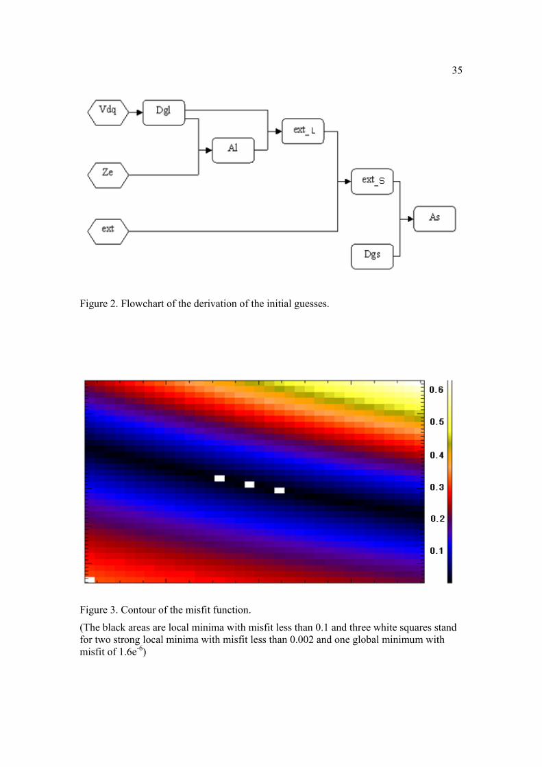
Now, with one initial guess gsD fixed as a constant temporarily, the initial guesses of
three PSD parameters lA , glD and sA are calculated from ,e dqZ V and extβ . The
procedure is summarized in Figure 2.
2.3.3 Two Problems in the Implementation In the implementation of the ideas discussed above, two problems need to be solved in
the retrieval algorithm.
First, in the derivation of the initial guesses of the PSD parameters, it is possible that
the large mode optical extinction calculated from the radar measurements is greater than
the total extinction estimated by the Raman lidar measurement. Considering the
instrument error in the radar and lidar measurements, and the assumptions made in the

22
forward model and the empirically derived power-law coefficients, this is a reasonable
occurrence and it suggests that a single PSD mode can be assumed when the difference
between the calculated and measured extinction is smaller than the combined error. In
other words, because a prominent small PSD mode would contribute significantly to the
extinction but not the radar measurements, a bimodal assumption is not needed when the
radar measurements can be used to reasonably approximate the measured lidar extinction.
When this situation is found, we implement an algorithm that uses three radar and lidar
measurements – radar reflectivity, Doppler velocity and lidar extinction, to retrieve a
single mode PSD but with three free parameters , and . The details of this
algorithm including the forward model equations are described in Appendix A: single
mode retrieval algorithm.
A second problem arises because only the lidar extinction is available to calculate two
small mode PSD parameters in the initial guesses, requiring us to fix either or .
The algorithm is quite sensitive to this choice because the cost function has several local
minima, and the Gauss Newton method is formulated to find an optimal solution for a
problem that is not very nonlinear (i.e., where a global minimum of the cost function is
easily identified).
So if the initial guess is not set properly, the Gauss Newton method reaches a local
minimum instead of the global minimum. For example, the sensitivity of the retrieval
results to parameter can be examined by using radar and lidar data simulated from
the forward model while fixing parameters and .
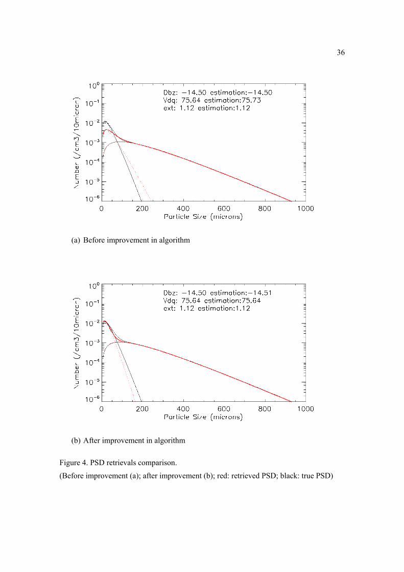
The contour of the misfit, which is the mean squared error (MSE) of the retrieved radar
and lidar data, is shown in Figure 3.
23
In Figure 3, we see several local minima with very small misfit that could be identified
by the optimal estimation method. Since the Gauss Newton method is simply designed to
identify a zero gradient condition, if the parameter Dgs is initially set to a value that is not
close to the actual solution, the Gauss Newton method could converge to one of these
local minima instead of the global minimum.
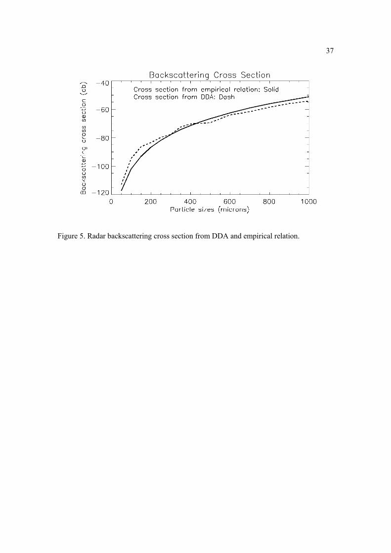
One simple and approximate solution to this problem is to iterate on the initial guess of
Dgs within a range of values, perform the algorithm using every initial guess, and choose
the one with the minimum misfit as the initial guess to be used in the retrieval algorithm.
After using this method, the accuracy of the retrieval algorithm is greatly improved. The
difference of particle size distribution retrievals before and after using this method is
shown in Figure 4.
This approach increases the computational expense of the algorithm. However, it
greatly increases the algorithm accuracy, and makes the algorithm capable of retrieving
high concentrations of small particles when appropriate.
2.4 Retrieval Uncertainty Evaluation An optimal solution and solution uncertainty are two fundamental requirements for an
inverse method (Wunsch, 2006). So a retrieval algorithm should not only be able to give
optimal estimates of desired quantities, but also provide estimation of how accurate the
retrieved quantities are. Rodgers (2000) shows that retrieval algorithm error sources can
be classified into four types: smoothing error, forward model error, model parameter
error, and measurement error.
According to Rodgers (2000), the smoothing error refers to the loss of information
24
from remote sensing systems' inability to see fine spatial structure. Since the actual
statistics of the fine structure being observed by Doppler radar and Raman lidar are
unknown, the retrieval here is an estimate of a smoothed version of the cloud state,
instead of an estimate of the complete state. So the smoothing error is not quantified here.
The forward model error is due to the approximations in the forward model
assumptions. For this study, they include the bimodal particle size distribution
assumptions, and also the Rayleigh scattering and Mie scattering assumptions used in the
forward model equations. Since the Rayleigh scattering and Mie scattering assumptions
are valid for 35 GHz radar and Raman lidar in measuring cirrus cloud reflectivity and
extinction as discussed before, the errors from Rayleigh and Mie scattering assumptions
should be small enough to be neglected.
For the error from the PSD assumption, DM06 shows that the two-parameter PSD
functions including exponential and gamma functions are applicable to retrieve particle
sizes when the actual PSD is not significantly bimodal. The two gamma functions are
sufficient to represent a small mode and a large mode PSD. The error from the bimodal
PSD model should also be small when the actual PSD is significantly bimodal.
In sum, the errors from bimodal PSD model assumptions and forward model
assumptions are both assumed small in this study relative to the known uncertainties in
the model parameters and measurements, so the forward model error is not considered
here either. In the following the retrieval errors from measurements and the empirical
model parameters are shown to be two major error sources, and they are discussed in
detail.
25
2.4.1 Measurement Error The total measurement error includes systematic error (due to instrument calibration)
and measurement noise, which is assumed to be random and unbiased. For radar
reflectivity, based on a known uncertainty in the MMCR radar reflectivity of
approximately 1-2 dBZ (Clothiaux et al., 1999; Miller, personal communication, 2001), a
25% error is applied to the radar reflectivity. Since the terminal fall velocity dqV is from
the retrieval of DM06 and their uncertainty estimation of retrieved dqV is about 30%,
this value is directly used as the measurement error for dqV in the error analysis.
Compared to radar measurement error, the measurement error for the lidar extinction
is quite variable; it strongly depends on factors like signal to noise ratio, laser power
fluctuations, and also the time of day (day time or night time). Since the error of the
extinction is estimated when the extinction is derived from the Raman lidar
measurements, the estimated error for lidar extinction is used in the algorithm. However,
to have a general idea of how accurate the derived lidar extinction is, the averaged
extinction error is calculated by using one year's data, and it is about 8.9% for daytime
and about 6.7% for night time.
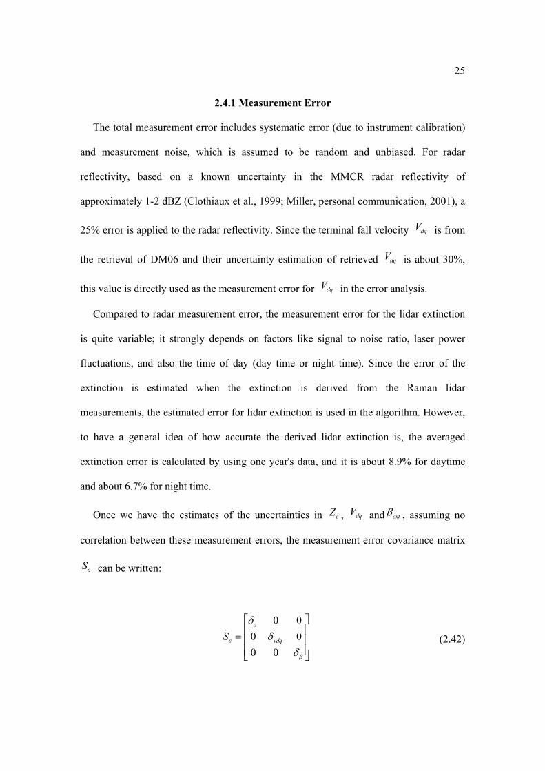
Once we have the estimates of the uncertainties in eZ , dqV and extβ , assuming no
correlation between these measurement errors, the measurement error covariance matrix
Sε can be written:
0 00 00 0
z
vdqSε
β
δδ
δ
⎡ ⎤⎢ ⎥= ⎢ ⎥⎢ ⎥⎣ ⎦
(2.42)
26
where zδ , vdqδ and βδ are the uncertainties for eZ , dqV and extβ respectively.
2.4.2 Power Law Model Parameter Error As mentioned in forward model equations, to express the radar and lidar
measurements as functions of PSD parameters only, six empirically derived power law
model parameters are used in the forward model equations, which are mass-dimensional
power law coefficients ma , mb , area-dimensional power law relationship coefficients
aa , ab , and terminal fall velocity parameters va , vb .
These model parameters are primarily dependent on the particle habits, and substantial
variations exist in these parameters when assuming different particle habits. For example,
za and zb are power law parameters to fit the radar backscattering cross section from
ice crystals with a certain shape. They can be derived from the mass-dimensional power
law coefficients ma , mb as shown in DM06. To see how well the radar cross section
(RCS) power-law fit is, the radar cross section ( )Dσ for a certain ice crystal shape can
be first calculated by using the Discrete Dipole Approximation (DDA) method (Donovan
et al., 2004; Liu, 2008) so that the RCS from power-law empirical parameters can be
compared with the numerical computation results. The comparison of the radar cross
section from power law fit and from the numerical method is shown in Figure 5. From
Figure 5, we see that the power law fit generally agrees well with the numerical results.
However, this agreement only happens when the particle habit is unique and the same as
what is used in the numerical computation. Since the ice crystal habit in cirrus is not
unique, and often is unknown, the error from these empirically derived power law
parameters used in the algorithm needs to be quantified.
27
To have a reasonable estimation of the errors in these parameters, the standard
deviations of the model parameters for different particle habits, as found in Mitchell
(1996), are used as the uncertainties of these model parameters.
In the calculation of the standard deviation, different particle habit groups are used for
the small mode and the large mode of the size distribution, considering the different
habits that the small and large particles may have. Specifically, five particle habits,
which include hexagonal plates, hexagonal columns, crystal with sector-like branches,
broad-branched crystal, and stellar crystal with broad arms are chosen for the small mode.
The mass- and area-dimensional model parameters ma , mb , aa and ab for the small
mode are listed in Table 1. Particle habits including hexagonal columns, side planes,
bullet rosettes with five branches, aggregates of side planes, columns and bullets are used
for the large mode. The mass- and area-dimensional model parameters for large mode
are listed in Table 2.
Because parameters av and bv can be derived from the air density, kinematic viscosity
and parameters ma , mb , aa , ab , as shown in Equations (2.10) and (2.11), and because
parameters za and zb can be expressed by the parameters ma and mb , as shown in
Equations (2.5) and (2.6), only the standard deviations for parameters ma , mb , aa , ab
need to be calculated for both the small mode and the large mode, which are listed in
Table 3.
Once the standard deviations for each model parameter are calculated, the model
parameter error covariance matrix mS can be written as:

28
0 0 0
0 0 0
0 0 0
0 0 0
m
m
a
a
a
b
a
b
δ
δ
δ
δ
⎡ ⎤⎢ ⎥⎢ ⎥= ⎢ ⎥⎢ ⎥⎢ ⎥⎣ ⎦
mS (2.43)
where maδ is a matrix 0
0ms
ml
a
a
δ
δ⎡ ⎤⎢ ⎥⎢ ⎥⎣ ⎦
, including the standard deviations for the small
mode parameter ams and the large mode parameter bms, and the same for mbδ , aaδ , abδ .
2.4.3 Retrieval Error Estimation Since the measurement error and the model parameter error are the two major errors,
Bayes’ theorem is used to quantify the retrieval error from these two error sources.
Following the derivation in Rodgers (2000), once the measurement error covariance
matrix εS and the model parameter error covariance matrix mS are given, the retrieval
error xS from εS and mS can be derived as:
( ) 11 1Ta
−− −= +x x d xS K S K S (2.44)
In Equation (2.44), dS is the total error covariance matrix, which includes the
instrument error covariance matrix εS and model parameter error covariance matrix Sm,
and it is written as:
T= +d ε m m mS S K S K (2.45)
where Km is the Jacobian matrix representing the sensitivity of the forward model to
29
model parameters, and is written as:
e e e e e e e e
ms ms ml ml as as al al
dq dq dq dq dq dq dq dq
ms ms ml ml as as al al
ext ext ext ext ext ext ext ext
ms ms ml ml as as al al
Z Z Z Z Z Z Z Za b a b a b a bV V V V V V V Va b a b a b a b
a b a b a b a bβ β β β β β β β
∂ ∂ ∂ ∂ ∂ ∂ ∂ ∂∂ ∂ ∂ ∂ ∂ ∂ ∂ ∂
∂ ∂ ∂ ∂ ∂ ∂ ∂ ∂
∂ ∂ ∂ ∂ ∂ ∂ ∂ ∂∂= =∂ ∂ ∂ ∂ ∂ ∂ ∂ ∂ ∂
∂ ∂ ∂ ∂ ∂ ∂ ∂ ∂
mFKm
ms ms ml ml as as al al
R R R R R R R Ra b a b a b a b
⎡ ⎤⎢ ⎥⎢ ⎥⎢ ⎥⎢ ⎥⎢ ⎥⎢ ⎥⎢ ⎥⎢ ⎥⎢ ⎥∂ ∂ ∂ ∂ ∂ ∂ ∂ ∂⎢ ⎥∂ ∂ ∂ ∂ ∂ ∂ ∂ ∂⎢ ⎥⎣ ⎦
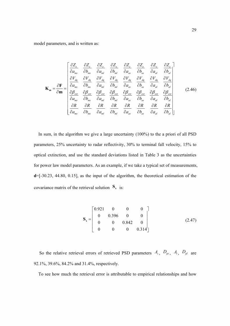
(2.46)
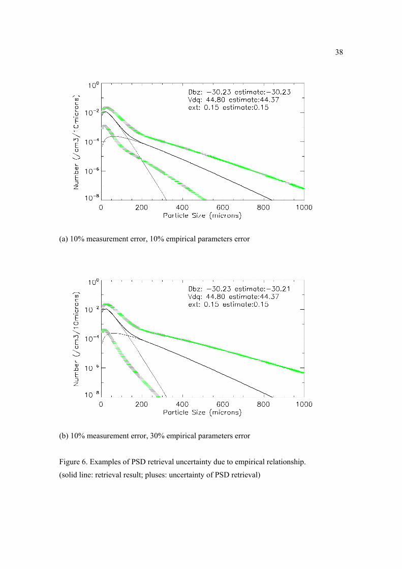
In sum, in the algorithm we give a large uncertainty (100%) to the a priori of all PSD
parameters, 25% uncertainty to radar reflectivity, 30% to terminal fall velocity, 15% to
optical extinction, and use the standard deviations listed in Table 3 as the uncertainties
for power law model parameters. As an example, if we take a typical set of measurements,
d=[-30.23, 44.80, 0.15], as the input of the algorithm, the theoretical estimation of the
covariance matrix of the retrieval solution xS is:
0.921 0 0 00 0.396 0 00 0 0.842 00 0 0 0.314
⎡ ⎤⎢ ⎥⎢ ⎥=⎢ ⎥⎢ ⎥⎣ ⎦
xS (2.47)
So the relative retrieval errors of retrieved PSD parameters sA , gsD , lA , glD are
92.1%, 39.6%, 84.2% and 31.4%, respectively.
To see how much the retrieval error is attributable to empirical relationships and how

30
much is due to measurement errors, a sensitivity test of the retrieval algorithm error to the
empirical relationships and measurement errors is given next.
2.4.4 Sensitivity Test From Equation (2.44), we see that the covariance of the solution vector x is
determined by the covariance of the measurement vector d and the covariance of the
empirical model parameter vector m. So the retrieval sensitivity to the measurement error
and the model parameter error are tested respectively in the following.
First, the sensitivity of the retrieval error to the model parameter error is tested by
varying the model parameter error and fixing the measurement error to 5%. Using the
same radar and lidar measurements mentioned above as the input of the algorithm, the
retrieval errors of four PSD parameters are given by Equation (2.44), and the errors of
IWC, and maximum dimension Dm can be calculated from Equations (2.21) and (2.22).
The retrieval errors from different modal parameter errors are listed in Table 4.
From Table 4, we can see, as the modal parameter covariance increases from 5% to
100%, the retrieval errors of all PSD parameters are increasing. The retrieval error of
mD increases from 16.6% to 72.4%, and the retrieval error of IWC increases from 77.5%
to 233.7%.
Fixing the model parameter covariance to 5%, and varying the measurement error, the
retrieval sensitivity to measurement errors is also tested. The retrieval error for
increases from 16.6% to 21.9%, and the retrieval error for IWC increases from 77.5% to
112.8%, as the measurement covariance increases from 5% to 100%.
The retrieval errors from different measurement errors are listed in Table 5, and the

31
retrieval errors of the PSD with different measurement and model parameter covariance
are shown in Figure 6. From Figure 6 and the comparison of Table 4 and Table 5, we
find that the retrieval errors are more sensitive to the uncertainty in empirical parameters
than to reasonable uncertainties in the measurements.
32
Table 1. Coefficients and exponents of mass-dimensional and area-dimensional relationships for small mode.
Particle Type Mass Area
am bm aa ba
Hexagonal Columns 0.1677 2.91 0.684 2.0
Bullet rosettes 0.00308 2.26 0.0869 1.57
Hexagonal Plates 0.00739 2.45 0.24 1.85
Crystal with branches 0.00614 2.42 0.24 1.85
Broad-branched Crystal 0.00583 2.42 0.24 1.85
Table 2. Coefficients and exponents of mass-dimensional and area-dimensional relationships for large mode.
Particle Type Mass Area
ma mb aa ab
Hexagonal Columns 0.000907 1.74 0.0512 1.414
Side Planes 0.00419 2.3 0.2285 1.88
Bullet rosettes 0.00308 2.26 0.0869 1.57
Aggregates 0.0028 2.1 0.2285 1.88
Hexagonal Plates 0.00739 2.45 0.65 2.0
33
Table 3. Means and standard deviations of mass-dimensional and area-dimensional power law parameters.
Mean Standard deviation Normalized STD
msa 0.0380 0.0649 1.7054
msb 2.4920 0.2453 0.0984
asa 0.2982 0.2256 0.7567
asb 1.8240 0.1561 0.0856
mla 0.0037 0.0024 0.6506
mlb 2.1700 0.2707 0.1248
ala 0.2490 0.2382 0.9567
alb 1.7488 0.2458 0.1405
Table 4. Sensitivity of retrieved PSD parameters to uncertainty in empirical relationships (5% Sε ,100% Sa).
Sm
Retrieval errors (%)
As Dgs Al Dgl IWC Dm
5% 72.3 18.8 60.2 19.9 77.5 16.6
10% 87.0 22.4 78.8 30.9 116.3 25.4
50% 97.6 25.5 95.4 73.4 217.3 60.1
100% 98.3 26.5 97.3 90.0 233.7 72.4
34
Table 5. Sensitivity of retrieved PSD parameters to uncertainty in measurements (5% Sm , 100% Sa).
Sε
Retrieval errors (%)
As Dgs Al Dgl IWC Dm
5% 72.3 18.8 60.2 19.9 77.5 16.6
10% 76.9 20.1 60.9 20.1 78.2 16.7
50% 93.1 23.6 75.4 22.6 94.7 18.2
100% 96.2 24.4 87.3 27.3 112.8 21.9
Figure 1. A bimodal particle size distribution with six parameters (Three parameters As, Dgs, αs control the small mode distribution, the other three parameters Al, Dgl, αl control the large mode distribution).
35
Figure 2. Flowchart of the derivation of the initial guesses.
Figure 3. Contour of the misfit function.
(The black areas are local minima with misfit less than 0.1 and three white squares stand for two strong local minima with misfit less than 0.002 and one global minimum with misfit of 1.6e-6)
36
(a) Before improvement in algorithm
(b) After improvement in algorithm
Figure 4. PSD retrievals comparison.
(Before improvement (a); after improvement (b); red: retrieved PSD; black: true PSD)
37
Figure 5. Radar backscattering cross section from DDA and empirical relation.
38
(a) 10% measurement error, 10% empirical parameters error
(b) 10% measurement error, 30% empirical parameters error
Figure 6. Examples of PSD retrieval uncertainty due to empirical relationship.
(solid line: retrieval result; pluses: uncertainty of PSD retrieval)

39
(c) 5% empirical parameters error, 10% measurement error
(d) 5% empirical parameters error, 100% measurement error
Figure 6. continued.

CHAPTER 3
CASE STUDY
In this chapter, the in situ measurements including the concentration and the IWC
collected by airborne instruments on board the UND Citation during the 2000 Cloud IOP
are used in the case study to compare with the retrievals from ground-based remote
sensing measurements. A statistical approach is first introduced for the comparison of
aircraft in situ measurements with retrieval from ground-based measurements to
minimize the differences in sample volume, and time and space between the two
platforms. Then the airborne instruments used in the case study and their problems are
discussed. After that, the PSD retrievals from ground-based remote sensing
measurements are compared with the PSD in situ measurements from the 2DC and the
FSSP, and the IWC retrievals are compared with the IWC measured by the CVI.
3.1 Comparing In Situ Measurements with Ground-Based Retrievals
3.1.1 Difficulties in Comparison Due to time, spatial and sample volume differences between the aircraft in situ
measurements and the ground-based remote sensing measurements, comparing aircraft in
situ measurements with retrievals from ground-based remote sensing measurements is
challenging. The difficulties of comparing aircraft in situ measurements with ground-
based remote sensing measurements are explored in earlier studies (e.g., Matrosov, 1997).
41
Here, the specific difficulties of comparing in situ measurements during horizontal flight
legs with retrievals from vertically pointing remote sensors are summarized, and a
method to overcome these difficulties is then proposed.
As mentioned in Mace et al. (2002), the sample volume of the MMCR at the ARM
SGP site is about 77000 m3 at 10 km. The sample volume rate of the PMS 2DC on the
UND Citation is about 6 liter s-1, so if using 5 seconds averages as is typical to get
reasonable aircraft sample statistics in the in situ probes, the sample volume of the
airborne instruments is only about 0.03 m3 (30 liters). There are six orders of magnitude
difference in the sample volumes between these two platforms for cirrus cloud at about
10 km altitude.
In addition to the large difference in sample volume, the spatial resolution of the
aircraft in situ measurements during horizontal flight legs and that of the remote sensing
measurements are also quite different. Specifically, for ground-based Raman lidar data,
its time resolution is about 10 minutes because of the need to smooth the noisy molecular
signal (Petty et al., 2006). Assuming that the cirrus clouds are moving at speeds of about
5-30 m s-1, the horizontal spatial dimension of the Raman lidar ranges from 3 to 18 km.
For the aircraft in situ measurements, assuming the aircraft is flying along a horizontal
leg at a speed of about 100 m s-1, the 5 seconds average of the in situ measurements
would provide a horizontal spatial resolution of about 500 m. So depending on the wind
speed and the aircraft speed, there exists a vast difference in horizontal spatial resolution
between aircraft in situ data and the ground-based Raman lidar data.
Because of the differences of the sample volume and the spatial resolution between the
airborne in situ measurements and the ground-based remote sensing measurements,

42
certain statistical approaches must be taken in order to make reasonable comparisons of
data collected from the two platforms.
3.1.2 Statistical Method The basic idea of this statistical approach relies on the fact that the aircraft flew
horizontal legs along the ambient wind direction. We also assume that any changes that
might occur between the time of measurement by the aircraft and when the remote
sensors measured the volume can be neglected. In situ measurements sampled at a
location that is more than 20 km away from the SGP site are not used in the comparison.
We consider each aircraft measurement (5 seconds average) to constitute an independent
sample and then we determine into which time-height remote sensing data bin the in situ
measurement can be most reasonably placed. The in situ data in each remote sensing bin
are then averaged to compare with the remote sensing retrieval. So the criteria used to
match the in situ measurement with the remote sensing bin are most important in this
statistical approach, and it is described in detail next.
First, since only the in situ measurements during horizontal legs are used in the
comparison, all in situ measurements during the same horizontal leg are made at
approximately a single altitude. After finding the average altitude of each leg, the in situ
measurements in each leg will only be compared with remote sensing retrievals at the
closest available range resolution volume. Because the vertical resolution of the MMCR
is 90 meters, the largest possible vertical spatial difference between remote sensing
retrievals and the aircraft in situ measurements is 45 m. In this way, measurements from
the two platforms should be close to each other in the vertical direction.

43
Second, the in situ measurements should also be close enough to the remote sensing
measurements in the horizontal plane. The coordinates of aircraft positions during the
first five horizontal legs are recorded by the GPS system, and are shown in Figure 7.
From Figure 7, we see that the UND Citation was flying close to the ARM SGP site
(N36°37', W97°30') several times. The closest approach happened at 20:56 UTC, with a
horizontal distance of 867 m from the aircraft to the SGP site. Although the aircraft never
passed directly over the exact location of the SGP site during the flight, compared to the 3
km to 18 km horizontal resolution of Raman lidar, 867 m distance is close enough. This
illustrates the difficulty of using high altitude aircraft to validate remote sensing
measurements and why a statistical approach is necessary.
The third step is to minimize the time difference between these two platforms. In
other words, we attempt to determine, given a time and location of in situ measurement,
what time the aircraft resolution volume was in the vicinity of the SGP remote sensors.
To be able to do that, the movement of the cirrus clouds is taken into account with the
help of sounding data. Because of the 10 minutes time resolution of the Raman lidar,
some part of the cloud sampled by the in situ instruments during the 10 minutes time
period may flow out of the cloud area measured by the Raman lidar, and some that are
sampled not during this 10 minutes may flow into the area, so the cloud movement must
be taken into account. Assuming in a short time period, such as 10 minutes, the cloud
system would only move with the wind without any significant changes in the cloud
structure, then the same cloud sampled by the aircraft at time ti will pass the SGP site at tj
or already passed the SGP site at tk depending on whether the aircraft is upwind or
downwind.

44
udtt ij /+= (3.1)
udtt ik /−= (3.2)
where u is the wind speed, which is acquired from interpolated sounding data, and d is
the distance from the aircraft to the SGP site, which can be calculated as:
2 | |/360 2 | |/360 (3.3)
where 1R and 2R are the equatorial and polar radius of the Earth, respectively, sθ and
sϕ are the latitude and longitude of the SGP site, respectively, θ and ϕ are the
latitude and longitude of the aircraft recorded by the GPS system.
By using the criteria discussed above, only the in situ measurements that are close
both in time and space to the remote sensing measurements are averaged to compare with
retrievals from the remote sensing measurements to account for the sampling difference
between the two platforms.
A primary problem with this comparison approach is that it will not work on rapid
change cloud systems, because in this approach, we assume that cirrus clouds do not have
significant changes in the cloud structure during the 10-minute intervals. And also, this
approach will not work on small scale cloud systems, because the horizontal scale of the
10-minute remote sensing intervals is on the order of km, not meters. So this method of
comparing airborne in situ measurements with ground-based remote sensing retrievals is
specifically designed for large horizontal scale cirrus cloud systems, in which case the

45
assumptions that we make in this approach are reasonable.
3.2 In Situ Measurements In this case study, the in situ measurements collected by different airborne instruments
on the UND Citation during the 2000 Cloud IOP are used. These instruments include
the Cloud Particle Imager (CPI), the PMS 2DC, the FSSP and the CVI. All the aircraft
instruments used in the case study are listed in Table 6; also listed are the in situ
measurements made by these airborne instruments. The measurements from these
airborne instruments and the problems in the measurements will be discussed in this
section.
3.2.1 Particle Images from the CPI The CPI images cloud particles in the size range of 20-2500 microns (maximum
dimension), with an image resolution of 2.3 micron. So from the analysis of the particle
images recorded by the CPI, the major particle habit of a cloud system can be deduced.
For example, based on the images taken by the CPI on March 9th, 2000, bullet rosettes are
found to be the predominant particle habit for the cirrus system on that day (Lewis et al.,
2001). Once the major particle habit is known, the corresponding mass- and area-
dimensional power law parameters will be used in the algorithm to retrieve the
microphysical properties including the particle number concentration and IWC to
compare with the in situ measurements.

46
3.2.2 Number Concentration from the 2DC and the FSSP One important in situ measurement to be verified by remote sensing retrievals is the
particle number concentration. The concentration in the range of 60-1500 µm is provided
by the PMS 2DC, and the concentration in the range of 2-47 µm can be provided by the
FSSP.
A problem with the PMS 2DC is the missampling of larger crystals due to the small
collection area of the instruments (Gayet et al., 1993). Because the concentrations of
larger particles in most thin cirrus clouds are very low, the PMS 2DC sample volume is
so small that the 2DC sensor may not have enough sample statistics, and thus may greatly
undercount the larger particles in its small sample volume. So it is a common approach to
average the individual samples of 2DC over a certain time period to improve the
sampling statistics. Five seconds is typically used to get reasonable sample statistics for
larger cirrus particles.
For the FSSP, the shattering effect on the concentration measurements of small
particles is discussed extensively in several recent papers (Heymsfield, 2007;
McFarquhar et al., 2007). Two possible physical mechanisms were proposed for the
particle shattering (Korolev and Isaac, 2005), and some studies used satellite retrievals to
show that the measurements from the FSSP may be biased due to the particle shattering.
However, since one motivation of this study is to see if the measurements from the FSSP
are biased or not, the original in situ measurements from the FSSP will be directly used
without any correction and compared with remote sensing retrievals.

47
3.2.3 Ice Water Content from the CVI Besides the measurements of the number concentration, the Ice Water Content (IWC)
was measured by the Counterflow Virtual Impactor (CVI) during the 2000 Cloud IOP.
The CVI uses a counterflow stream of gas to separate cloud droplets or ice crystals from
the interstitial aerosol and water vapor. The details of this instrument can be found in
Twohy et al. (1997).
One issue that would affect the accuracy of the IWC measurements from the CVI is
that there is a minimum size of ice particle that can penetrate the counterflow and
penetrate the inside of the CVI inlet. As mentioned in Twohy et al. (1997), the
minimum size of a cloud particle that is able to enter the CVI inlet tip is dependent on
particle velocity, inlet size, and the CVI counterflow rate. The minimum particle diameter
collected with 50% efficiency, also known as the “cut size” is about 7 microns aero-
dynamic diameter (diameter of a unit-density sphere) for the NCAR CVI at sea level.
According to Twohy et al. (2003), the cut sizes of the CVI at the airspeeds of 100 and 67
m s-1 are 8.2 and 9.6 microns aero-dynamic diameter, respectively.
To have an idea about the corresponding cut sizes in maximum dimension (D) as used
in the retrieval algorithm, the aerodynamic diameter (Da) can be converted to the
maximum dimension (D) by the formalism in Appendix B.
According to Equation (B4) in Appendix B, using 0.91 g cm-3 as the unit density for
solid ice sphere, and using the effective density versus D relationship representing the
rosettes from Heymsfield et al. (2003), the relationship between the aero-dynamic
diameter aD and the maximum dimension D can be expressed as:

48
3 0.3937(34.34 )aD D= (3.4)
So assuming a bullet rosette particle habit, the cut sizes of the CVI at the airspeeds of
100 and 67 m s-1 are 48.3 and 58.2 microns in maximum dimension. That is to say the
CVI has reduced collection efficiency (50%) of cloud droplets or ice crystals for cloud
particles with a maximum dimension of about 50 microns. This reduced collection
efficiency for small cloud particles of CVI may have a small effect on the IWC
measurements from the CVI, which will be discussed next.
3.3 Case Study on March 9th 2000 The statistical approach discussed in section 3.1 and the in situ measurements
introduced in section 3.2 are here used in the comparison of retrievals from ground-based
remote sensing measurements and aircraft in situ measurements made on March 9th, 2000.
The synoptic situation and aircraft flight information on that day are briefly introduced
first, and then the PSD comparison and IWC comparison results are discussed.
3.3.1 Synopsis and Flight Information On March 9th 2000, there was a southwestern jet to the west of the ARM SGP Central
Facility. Heymsfield et al. (2002) gives the following information about the cirrus that
developed and advected over the SGP site: “A dynamically active band of cirrus, with
embedded generating cells and trails (cirrrus uncinus) moved over the operations area on
March 9th 2000, producing almost exclusively single rosettes and aggregates of rosettes
suitable for study.”

49
For the flight of the UND Citation, the following description is given by Mace et al.
(2002): “The Citation began collecting data along 75 km level legs centered on the CART
site near cloud top (9.4 km) at approximately 19:20 UTC. During the ensuing 90 minutes,
the Citation conducted 5 level legs, stepping down through the cloud layer during the
period. ” The radar reflectivity and the flight path of the UND Citation on March 9th 2000
are shown in Figure 8.
3.3.2 Comparison of PSD Using the statistical approach mention in section 3.1, the PSD retrievals from the
algorithm discussed in Chapter 2 are compared with in situ measurements from the PMS
2DC and the FSSP during the first five horizontal legs of the UND Citation on March 9th,
2000. However, due to the 10-minute time resolution of the Raman lidar, there are only
seven retrieval results available for comparison during the five horizontal legs, which are
shown as the red X’s in Figure 8. However, the second and the third PSD retrievals on
the second horizontal leg show strong bimodality, and the comparisons with in situ
measurements are shown in Figure 9 (a) and (b). In Figure 9, the green envelope is the
uncertainty of PSD retrievals (calculated from the retrieval uncertainties of PSD
parameters) estimated by the optimal estimation method from the radar and lidar
measurement errors and the empirically derived model parameter errors.
Since bullet rosette is the predominant particle habit on March 9th 2000, the mass and
area-dimensional parameters for five branched bullet rosettes in Mitchell (1996) are used
in the algorithm. The uncertainties for these model parameters are assumed to be within
20%, and the uncertainties for eZ , dqV , extβ are assumed to be 25%, 30%, and 20%,
50
respectively, as discussed in Chapter 2.
The blue lines in Figure 9 show all 5 seconds averaged in situ measurements selected
using the statistical method discussed in section 3.1 to compare with the remote sensing
retrievals. We find that for large particles, most PSD in situ measurements from the 2DC
fall inside the retrieval uncertainty envelope, and the averaged PSDs agree well with the
large mode PSD retrievals. However, for sub-50 micron small particles, the averaged
concentration of small particles from the FSSP is about 10 times larger than that of the
retrieved small mode concentration, and all in situ PSD measurements from the FSSP
used in the average are outside the retrieval uncertainty envelope.
So from the above comparison of bimodal PSD retrieval and PSD in situ
measurements from 2DC and FSSP, we find that the large mode PSD retrievals from the
ground-based remote sensing measurements agree well with PSD from 2DC. However,
the small mode PSD retrievals are not consistent with the high concentrations of small
particles measured by the FSSP. The other five comparisons of PSD during the horizontal
flight legs are shown in Figure 10.
In these cases, only one large mode PSD is retrieved by the algorithm from the radar
and lidar measurements because, given the radar reflectivity measurements and the
terminal fall velocity retrieval, the extinction calculated for the first guess is less than or
equal to the extinction retrieved from the Raman lidar. Therefore, the small mode PSD is
not necessary and not appropriate to be included for the optimal estimation method to
retrieve the optical extinction from the Raman lidar.
For these PSD comparisons, the PSD retrievals also agree well with the averaged 2DC
in situ measurements, and most 2DC in situ measurements used in the average fall inside
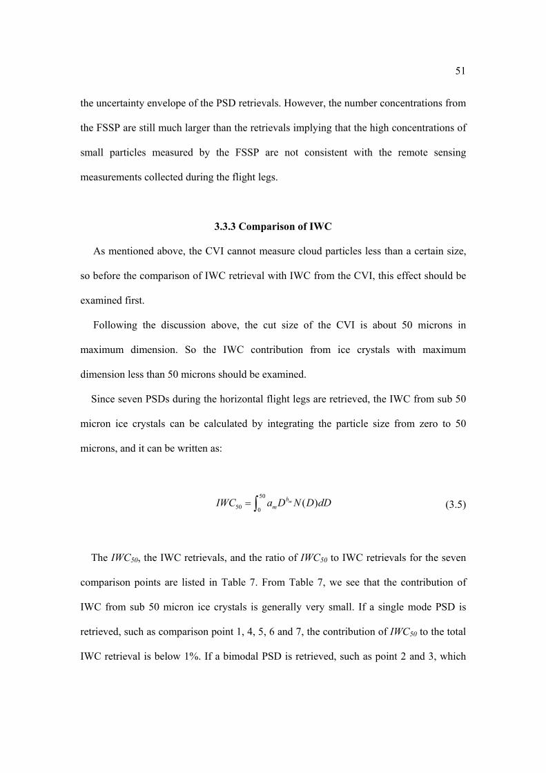
51
the uncertainty envelope of the PSD retrievals. However, the number concentrations from
the FSSP are still much larger than the retrievals implying that the high concentrations of
small particles measured by the FSSP are not consistent with the remote sensing
measurements collected during the flight legs.
3.3.3 Comparison of IWC As mentioned above, the CVI cannot measure cloud particles less than a certain size,
so before the comparison of IWC retrieval with IWC from the CVI, this effect should be
examined first.
Following the discussion above, the cut size of the CVI is about 50 microns in
maximum dimension. So the IWC contribution from ice crystals with maximum
dimension less than 50 microns should be examined.
Since seven PSDs during the horizontal flight legs are retrieved, the IWC from sub 50
micron ice crystals can be calculated by integrating the particle size from zero to 50
microns, and it can be written as:
50
50 0( )mb
mIWC a D N D dD= ∫ (3.5)
The IWC50, the IWC retrievals, and the ratio of IWC50 to IWC retrievals for the seven
comparison points are listed in Table 7. From Table 7, we see that the contribution of
IWC from sub 50 micron ice crystals is generally very small. If a single mode PSD is
retrieved, such as comparison point 1, 4, 5, 6 and 7, the contribution of IWC50 to the total
IWC retrieval is below 1%. If a bimodal PSD is retrieved, such as point 2 and 3, which
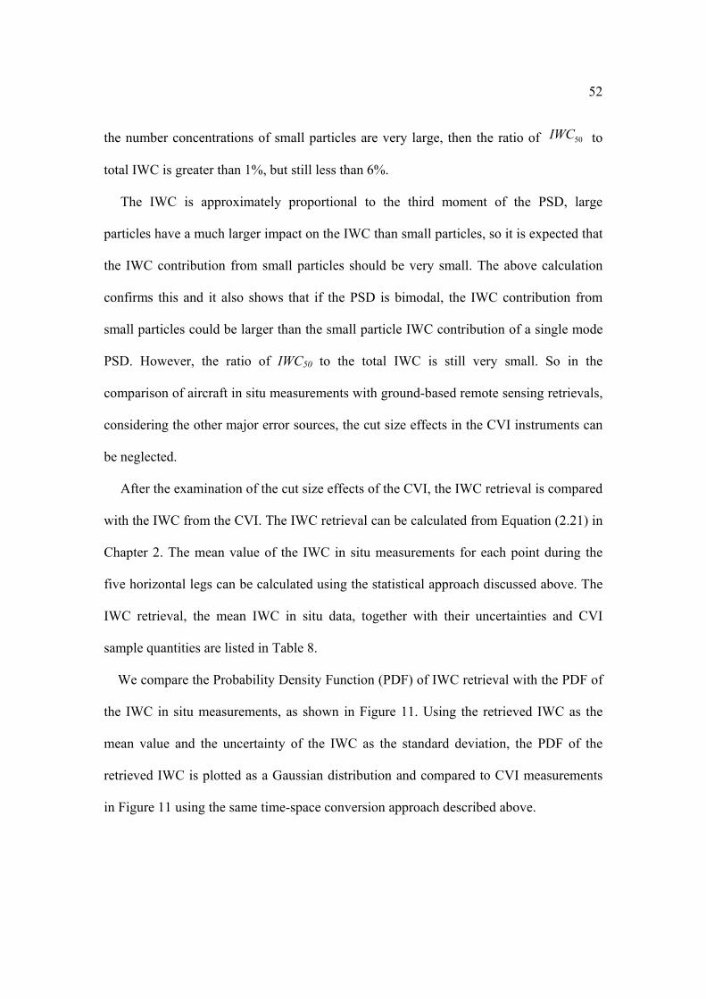
52
the number concentrations of small particles are very large, then the ratio of 50IWC to
total IWC is greater than 1%, but still less than 6%.
The IWC is approximately proportional to the third moment of the PSD, large
particles have a much larger impact on the IWC than small particles, so it is expected that
the IWC contribution from small particles should be very small. The above calculation
confirms this and it also shows that if the PSD is bimodal, the IWC contribution from
small particles could be larger than the small particle IWC contribution of a single mode
PSD. However, the ratio of IWC50 to the total IWC is still very small. So in the
comparison of aircraft in situ measurements with ground-based remote sensing retrievals,
considering the other major error sources, the cut size effects in the CVI instruments can
be neglected.
After the examination of the cut size effects of the CVI, the IWC retrieval is compared
with the IWC from the CVI. The IWC retrieval can be calculated from Equation (2.21) in
Chapter 2. The mean value of the IWC in situ measurements for each point during the
five horizontal legs can be calculated using the statistical approach discussed above. The
IWC retrieval, the mean IWC in situ data, together with their uncertainties and CVI
sample quantities are listed in Table 8.
We compare the Probability Density Function (PDF) of IWC retrieval with the PDF of
the IWC in situ measurements, as shown in Figure 11. Using the retrieved IWC as the
mean value and the uncertainty of the IWC as the standard deviation, the PDF of the
retrieved IWC is plotted as a Gaussian distribution and compared to CVI measurements
in Figure 11 using the same time-space conversion approach described above.
53
For the first point, there are only three in situ IWC samples selected by the statistical
method, and they are all close to the mean value of the retrieval. For the second point,
most in situ samples fall inside the three sigma area of the Gaussian PDF of the retrieval.
However, for the rest of the points, several of the in situ samples are outside the three
sigma area of the retrieval PDFs. Therefore, the means of the in situ measurements do
not agree well with the retrieval results, as shown in Table 8. However, for all the
comparison points, the peaks of the in situ measurement PDFs are within the retrieval
PDFs.

54
Table 6. UND Citation Instruments and measurements.
Instruments Measurements
Forward Scatter Spectrometer Probe Size distribution (2-47 µm)
PMS 2 Dimension Cloud Probe Size Distribution (60-1500 µm)
Counterflow Virtual Impacter Ice Water Content
Cloud Particle Imager Particle images (used for particle habits)
Table 7. Percentage of IWC50 in the total IWC.
IWC50 (g m-3) IWC total (g m-3) IWC50/ IWC
1 2.796e-5 6.007e-3 0.47%
2 11.752e-5 2.325 e-3 5.05%
3 11.245e-5 5.244 e-3 2.14%
4 1.386e-5 5.641 e-3 0.25%
5 1.519e-5 5.350 e-3 0.28%
6 1.059e-5 2.323 e-3 0.46%
7 0.679e-5 1.617 e-3 0.42%

55
Table 8. The mean and standard deviation for IWC in situ data and IWC retrieval. In situ measurements Retrievals
Mean
(g/m3)
STD
(g/m3)
Sample
number
Solution
(g/m3)
Uncertainty
1 0.0044 0.0037 3 0.0060 90%
2 0.0033 0.0028 29 0.0023 80%
3 0.0119 0.0069 27 0.0052 93%
4 0.0223 0.0129 17 0.0056 90%
5 0.0113 0.0093 29 0.0054 90%
6 0.0083 0.0068 24 0.0023 88%
7 0.0073 0.0079 38 0.0016 56%
Figure 7. Coordinates of the airplane positions during the first five legs.
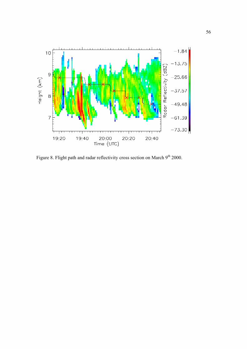
56
Figure 8. Flight path and radar reflectivity cross section on March 9th 2000.
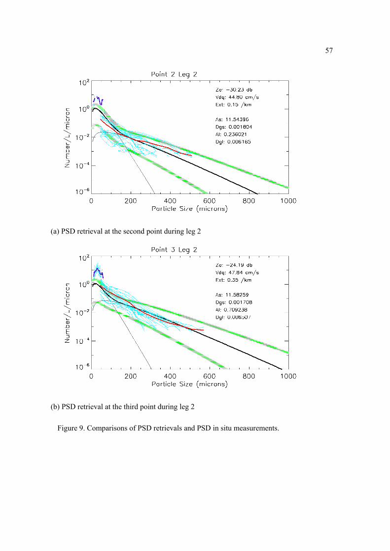
57
(a) PSD retrieval at the second point during leg 2
(b) PSD retrieval at the third point during leg 2
Figure 9. Comparisons of PSD retrievals and PSD in situ measurements.

58
(a) Point 1
(b) Point 4
Figure 10. Comparisons of single mode PSD retrievals with in situ data.
(Point 1: (a); Point 4: (b); Point 5: (c); Point 6: (d); Point 7: (e))
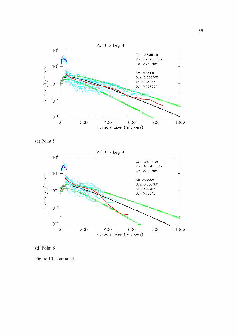
59
(c) Point 5
(d) Point 6
Figure 10. continued.

60
(e) Point 7
Figure 10. continued.
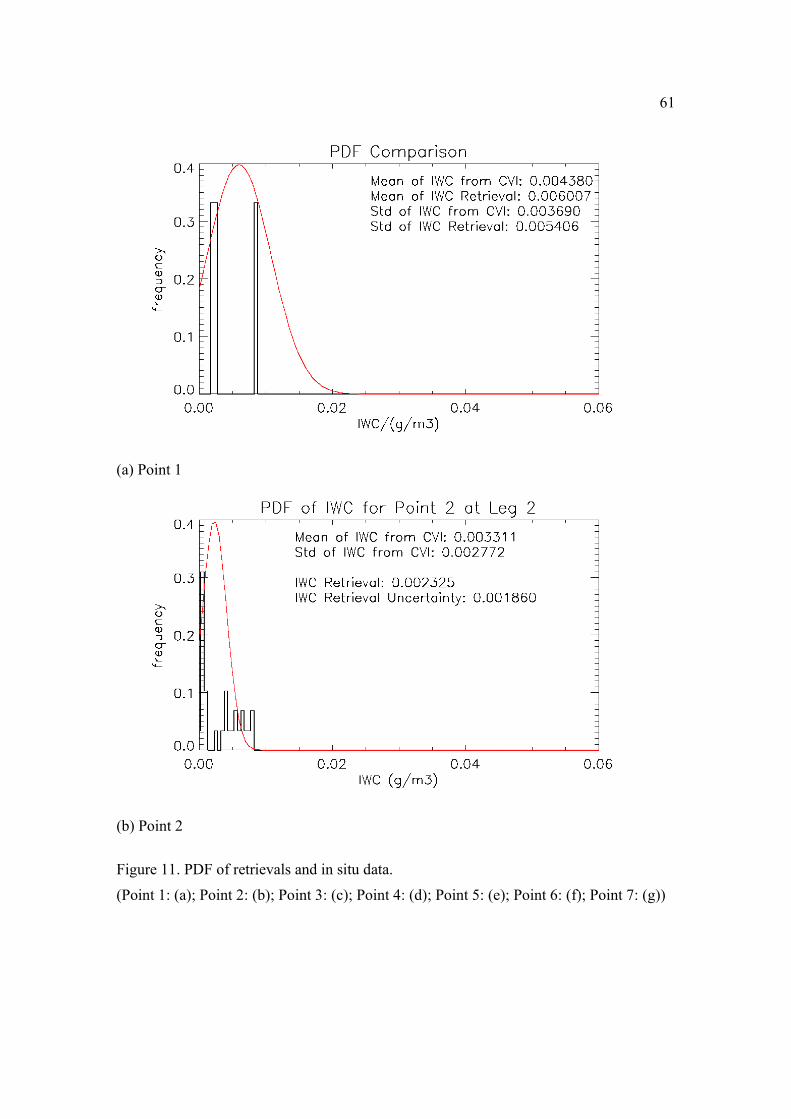
61
(a) Point 1
(b) Point 2
Figure 11. PDF of retrievals and in situ data.
(Point 1: (a); Point 2: (b); Point 3: (c); Point 4: (d); Point 5: (e); Point 6: (f); Point 7: (g))

62
(c) Point 3
(d) Point 4
Figure 11. Continued.
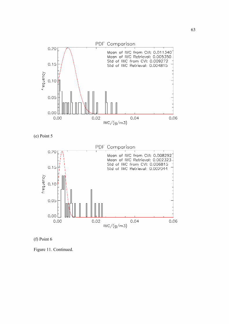
63
(e) Point 5
(f) Point 6
Figure 11. Continued.
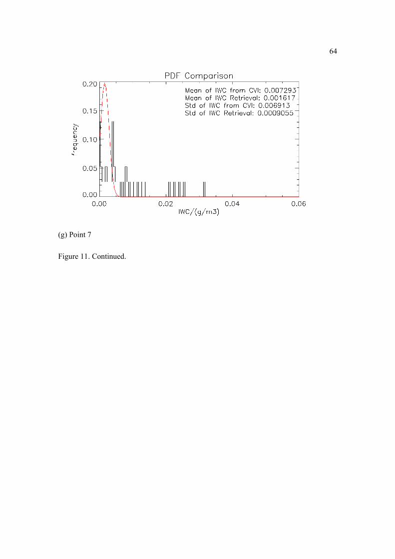
64
(g) Point 7
Figure 11. Continued.
CHAPTER 4
ONE-YEAR STATISTICS Many recent studies using aircraft in situ measurements (e.g., Lawson et al., 2006)
show that the average particle concentrations in midlatitude cirrus clouds are on the order
of 1 cm-3. However, other studies (Heymsfield, 2007; McFarquhar et al., 2007) suggest
that the cirrus microphysical statistics derived from aircraft in situ measurements may be
biased due to an artificial enhancement in small ice crystals from the shattering of larger
ice crystals on aircraft and probe surfaces. To see if the cirrus statistics from aircraft in
situ measurements are consistent with that from remote sensing retrievals, appropriately
formulated retrieval algorithms need to be applied to long-term remote sensing
measurements. The cirrus statistics from long-term remote sensing retrievals have been
derived by only a few studies (Mace et al., 2006; Deng and Mace 2008). However, the
algorithms used in those studies were not capable of retrieving high concentrations of
small crystals because of an assumption of a single mode PSD. An algorithm that is
capable of retrieving a bimodal PSD similar to what is typically seen in aircraft data, and
thus can represent microphysical properties for both small particles and large particles,
has never been applied to long-term ground-based remote sensing measurements. In this
chapter, the algorithm described in Chapter 2 is applied to 313-hour cirrus events
observed at the ARM SGP site, and 33641 retrievals are used to study cirrus
microphysical statistics.

66
4.1 PSD Bimodality Statistics The existence of bimodality indicates certain microphysical processes, such as
secondary nucleation of ice crystals within a cirrus layer (Comstock et al., 2008). The
presence of significant bimodality also has implications for cirrus cloud property
retrievals from ground-based and space-based sensors. We emphasize the word
“significant” because quite often the algorithm used in this study diagnoses a PSD that
utilizes both gamma functions to best represent the data. However, quite often a unimodal
description of the PSD would be sufficient to describe, to within some specified degree of
uncertainty, the PSD moments that are most relevant to the integrated physical quantities
such as IWC, effective radius, and extinction. Previous studies, such as Mace et al.
(2002), used aircraft in situ data to study the frequency of occurrence of bimodal size
distributions in cirrus. However, an examination of bimodality has never been applied to
long-term remote sensing measurements.
The approach that we take is to fit the retrieved PSD using unimodal distribution
functions and then to use the misfit between the PSD retrieval and the fitted PSD to
ascertain the degree of bimodality of the PSD. A modified gamma function with three
degrees of freedom is used as the fitting function. The difference of the second, third and
fifth moments of the retrieved PSD and the fitted gamma function is used as the cost
function, which is written in Equation (4.1).
2 22
3 3 5 52 2
2 3 5
' ''f μ μ μ μμ μμ μ μ
− −−= + + (4.1)

67
where 2 'μ , 3 'μ , 5 'μ are the second moment, the third moment and the fifth moment
of the fitted PSD, respectively, and 2μ , 3μ , 5μ are the second moment, the third
moment and the fifth moment of the PSD retrieval.
Because the second, third and fifth moment approximately correspond to the
extinction, the IWC and the radar reflectivity, respectively, the difference between the
PSD retrieval and the unimodal PSD function can be measured by these quantities with
actual physical meanings. Once the fitting function and the cost function are chosen, the
amoeba algorithm, which is a commonly used nonlinear optimization algorithm (Nelder
and Mead, 1965), is used in the minimization. The misfit between the fitted PSD and the
PSD retrieval can be calculated from the cost function expressed in Equation (4.1).
Finally, a threshold value for the misfit needs to be set to distinguish a strong bimodal
PSD retrieval from a single mode PSD retrieval or a weak bimodal PSD retrieval. Many
PSD retrievals have been investigated to find a proper threshold for strong bimodal PSD,
and four examples are shown in Figure 12. In the first PSD example shown in Figure 12
(a), the magnitude of the small mode PSD is very small. The misfit between the gamma
function fit and the bimodal PSD is only 1%. The misfit of the second PSD example
increases to 10%, the bimodality also increases, but it is still a weak bimodal PSD. In
Figure 12 (c) and Figure 12 (d), the PSD retrievals show stronger bimodality. One
gamma function cannot represent the bimodal PSD, and the misfits are 20% and 30%,
respectively. From the above and other examples that we have studied, 30% is chosen to
be a proper threshold to distinguish a strong bimodal PSD from a unimodal PSD or a
weak bimodal PSD. This value of misfit is approximately the degree of uncertainty that
one would expect in retrieving the PSD moments from either remote sensing data or from

68
in situ data and so is an appropriate threshold metric for our purposes.
After defining a proper and physically meaningful way to measure PSD bimodality,
the variation of the PSD bimodality with the environmental temperature and radar
reflectivity is explored by using 33641 ground-based remote sensing retrievals.
The histogram of the bimodality frequency in terms of radar reflectivity and
temperature is shown in Figure 13. The bimodality frequencies for cirrus with very small
radar reflectivities (less than -35 dBZ) at very low temperatures (lower than 230 K) are
generally below 25%. As the temperature increases, the bimodality frequency also
increases. However, when radar reflectivity is above -15 dBZ, the bimodality frequency
is generally less than 20%, regardless of the temperature. A bimodality occurrence
frequency of more than 40% only happens when the temperature is above 240K and radar
reflectivity is below -15 dBZ. If the temperature is below 240K, the bimodality frequency
is generally less than 30%. The bimodality frequency histogram shows a dependency of
PSD bimodality on temperature when the radar reflectivity is less than -15 dBZ, and this
dependency is shown again in the bimodality frequency vertical profile in Figure 14. In
Figure 14, the bimodality frequency profiles are plotted separately for cirrus with
different temperature ranges. Cirrus with temperature less than 223K (coldest cirrus) is
shown in black, cirrus with temperature between 223K and 243K is in green, and the
warmest cirrus with temperature higher than 243K is shown in red.
For the coldest cirrus, the bimodality frequencies are all below 20%, and the profile
does not change much from the cloud bottom, where the normalized height (Mace et al.,
1997) is zero, to the cloud top, where the normalized height is unity. However, for the
warmest cirrus, the bimodality frequency drops rapidly from more than 40% at the cloud

69
top to less than 20% in the lower half of the profile, and then increases to about 40% near
the cloud base. The decrease in the bimodality frequency for the warmest cirrus in the
upper half of the profile may be related to the heterogeneous nucleation of new ice
crystals as larger crystals sediment through the layer. Small ice crystals and middle-sized
ice crystals at the cloud top tend to form larger-sized ice crystals, which would dominate
the total population of the ice crystals.
4.2 PDFs of IWC, Effective Radius and Concentration
4.2.1 PDF of IWC The PDFs of the IWC retrieval, shown in Figure 15, demonstrate a clear dependence
on temperature (e.g., Heymsfield and Platt, 1984) in their mean, mode, and variance.
The coldest third of cirrus (T < 223K; hereafter coldest cirrus) has the lowest IWC
mean value, about 1.61 mg m-3 with a standard deviation (STD) of 2.69 mg m-3 The
warmest third of cirrus (T > 243K; hereafter warmest cirrus) has the highest mean value,
which is 12.60 mg m-3with a standard deviation of 17.07 mg m-3. The middle-temperature
cirrus (223K < T < 243K) has a mean IWC of 6.09 mg m-3 (standard deviation of 10.56
mg m-3), which is in the middle of the mean IWC of the warmest cirrus and the coldest
cirrus. Consistent with the mean value, the PDF of the coldest cirrus is the narrowest,
extending from 0.1 mg m-3 to about one mg m-3; but for the warmest cirrus, the PDF
extends across the entire range from 0.1 mg m-3 to hundreds of mg m-3.
The modal values of IWC also increase substantially with temperature. The coldest
cirrus has a very large and narrow maximum with a peak frequency of almost 25%,
which means that almost 25% of IWC that the coldest cirrus has is among the range of
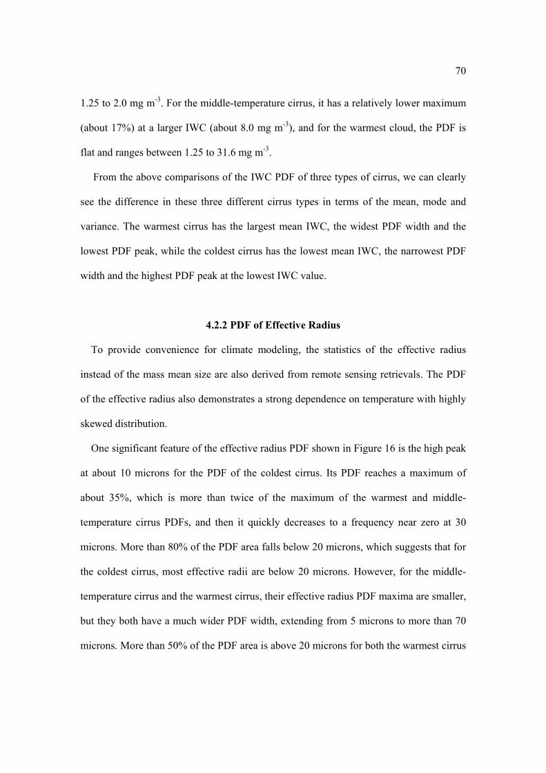
70
1.25 to 2.0 mg m-3. For the middle-temperature cirrus, it has a relatively lower maximum
(about 17%) at a larger IWC (about 8.0 mg m-3), and for the warmest cloud, the PDF is
flat and ranges between 1.25 to 31.6 mg m-3.
From the above comparisons of the IWC PDF of three types of cirrus, we can clearly
see the difference in these three different cirrus types in terms of the mean, mode and
variance. The warmest cirrus has the largest mean IWC, the widest PDF width and the
lowest PDF peak, while the coldest cirrus has the lowest mean IWC, the narrowest PDF
width and the highest PDF peak at the lowest IWC value.
4.2.2 PDF of Effective Radius To provide convenience for climate modeling, the statistics of the effective radius
instead of the mass mean size are also derived from remote sensing retrievals. The PDF
of the effective radius also demonstrates a strong dependence on temperature with highly
skewed distribution.
One significant feature of the effective radius PDF shown in Figure 16 is the high peak
at about 10 microns for the PDF of the coldest cirrus. Its PDF reaches a maximum of
about 35%, which is more than twice of the maximum of the warmest and middle-
temperature cirrus PDFs, and then it quickly decreases to a frequency near zero at 30
microns. More than 80% of the PDF area falls below 20 microns, which suggests that for
the coldest cirrus, most effective radii are below 20 microns. However, for the middle-
temperature cirrus and the warmest cirrus, their effective radius PDF maxima are smaller,
but they both have a much wider PDF width, extending from 5 microns to more than 70
microns. More than 50% of the PDF area is above 20 microns for both the warmest cirrus
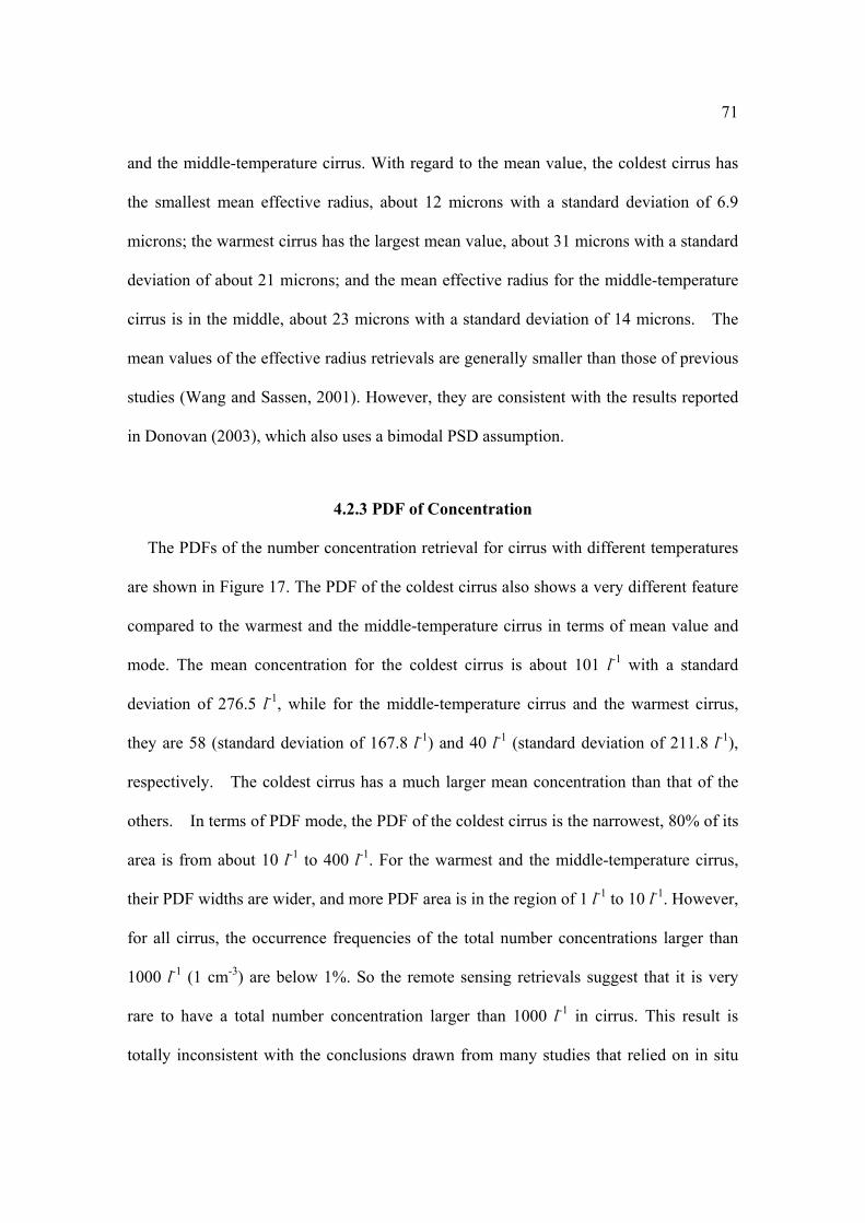
71
and the middle-temperature cirrus. With regard to the mean value, the coldest cirrus has
the smallest mean effective radius, about 12 microns with a standard deviation of 6.9
microns; the warmest cirrus has the largest mean value, about 31 microns with a standard
deviation of about 21 microns; and the mean effective radius for the middle-temperature
cirrus is in the middle, about 23 microns with a standard deviation of 14 microns. The
mean values of the effective radius retrievals are generally smaller than those of previous
studies (Wang and Sassen, 2001). However, they are consistent with the results reported
in Donovan (2003), which also uses a bimodal PSD assumption.
4.2.3 PDF of Concentration The PDFs of the number concentration retrieval for cirrus with different temperatures
are shown in Figure 17. The PDF of the coldest cirrus also shows a very different feature
compared to the warmest and the middle-temperature cirrus in terms of mean value and
mode. The mean concentration for the coldest cirrus is about 101 l-1 with a standard
deviation of 276.5 l-1, while for the middle-temperature cirrus and the warmest cirrus,
they are 58 (standard deviation of 167.8 l-1) and 40 l-1 (standard deviation of 211.8 l-1),
respectively. The coldest cirrus has a much larger mean concentration than that of the
others. In terms of PDF mode, the PDF of the coldest cirrus is the narrowest, 80% of its
area is from about 10 l-1 to 400 l-1. For the warmest and the middle-temperature cirrus,
their PDF widths are wider, and more PDF area is in the region of 1 l-1 to 10 l-1. However,
for all cirrus, the occurrence frequencies of the total number concentrations larger than
1000 l-1 (1 cm-3) are below 1%. So the remote sensing retrievals suggest that it is very
rare to have a total number concentration larger than 1000 l-1 in cirrus. This result is
totally inconsistent with the conclusions drawn from many studies that relied on in situ
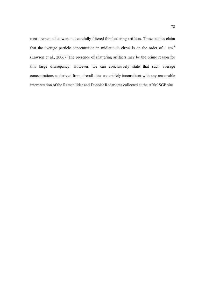
72
measurements that were not carefully filtered for shattering artifacts. These studies claim
that the average particle concentration in midlatitude cirrus is on the order of 1 cm-3
(Lawson et al., 2006). The presence of shattering artifacts may be the prime reason for
this large discrepancy. However, we can conclusively state that such average
concentrations as derived from aircraft data are entirely inconsistent with any reasonable
interpretation of the Raman lidar and Doppler Radar data collected at the ARM SGP site.
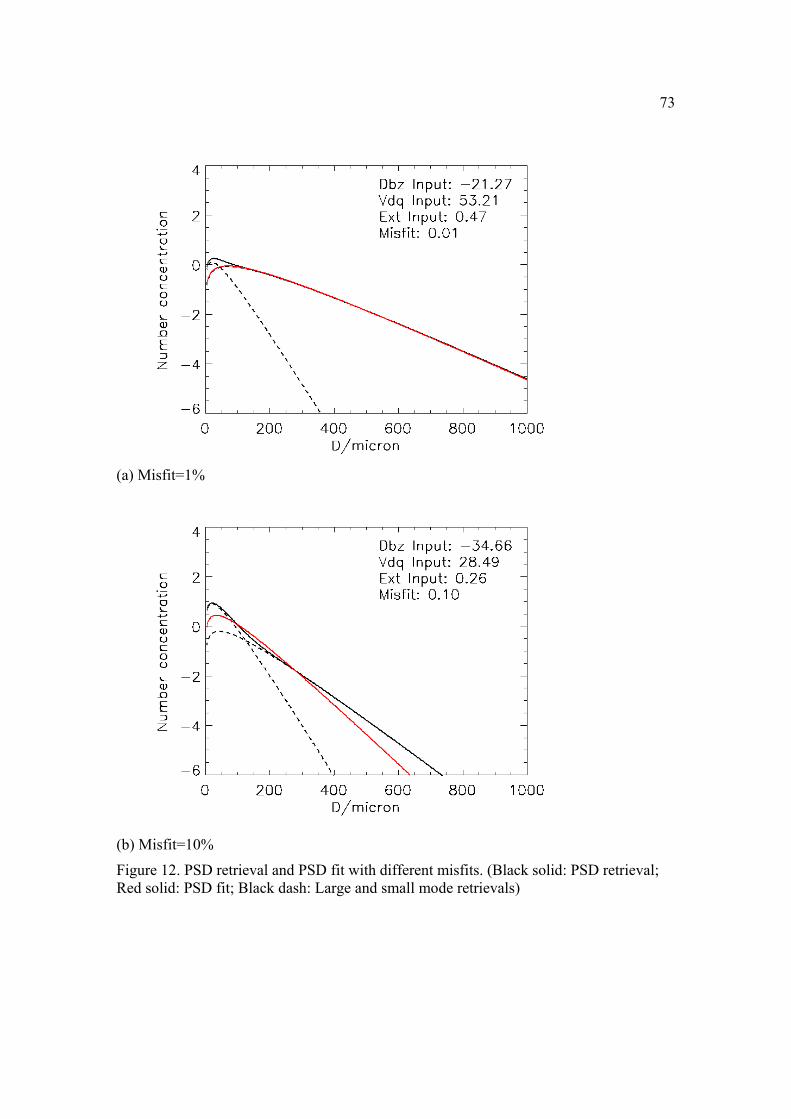
73
(a) Misfit=1%
(b) Misfit=10%
Figure 12. PSD retrieval and PSD fit with different misfits. (Black solid: PSD retrieval; Red solid: PSD fit; Black dash: Large and small mode retrievals)

74
(c) Misfit=20%
(d) Misfit=30%
Figure 12. continued.
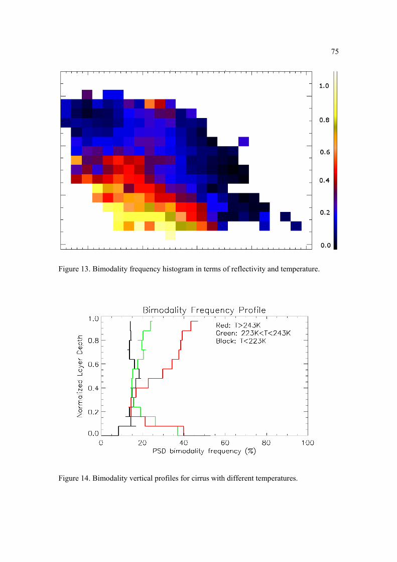
75
Figure 13. Bimodality frequency histogram in terms of reflectivity and temperature.
Figure 14. Bimodality vertical profiles for cirrus with different temperatures.
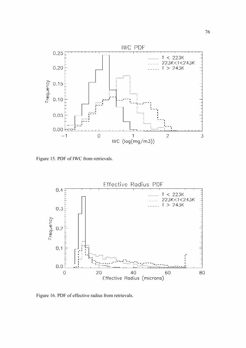
76
Figure 15. PDF of IWC from retrievals.
Figure 16. PDF of effective radius from retrievals.
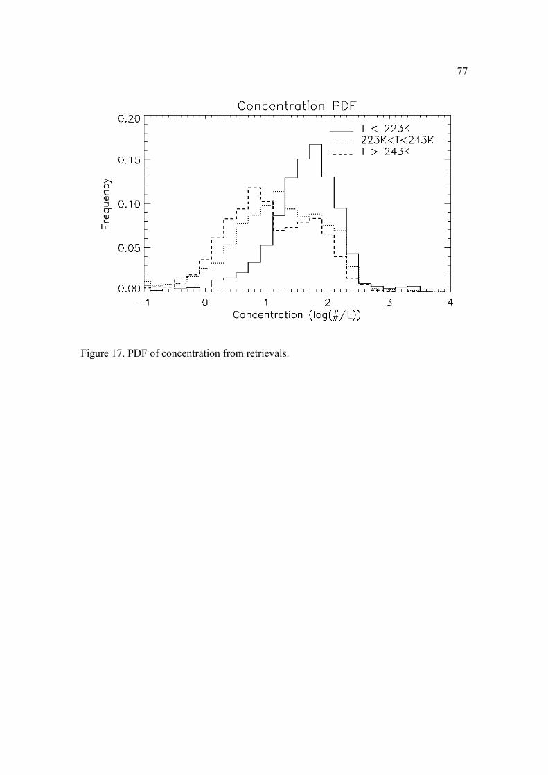
77
Figure 17. PDF of concentration from retrievals.

CHAPTER 5
SUMMARY
To better understand the feedback by cirrus clouds on the climate system, both the
macrophysical and microphysical properties of cirrus must be quantified. At the
microphysical level, how light is scattered by ice crystals, especially small ice crystals, is
critically important to the solar radiative properties of the cirrus cloud. So to better
quantify the scattering effects of ice crystals, many field experiments have been
conducted and many in situ measurements have been made. Recent studies suggest that
some aircraft in situ measurements, such as measurements from the FSSP, may be
contaminated by ice crystal shattering on probe inlets and aircraft surfaces. The potential
for shattering artifacts has called into question the validity of the aircraft data.
The motivation for this study is to see if the aircraft in situ measurements are
consistent with ground-based remote sensing measurements. The aircraft in situ data used
in this study is from the 2000 Spring Cloud IOP, and the data include the particle images
from the CPI, the IWC from the CVI, and the number concentration measurements for
small particles from the FSSP and those for large particles from the 2DC. The remote
sensing data used in the retrieval algorithm includes the optical extinction estimation
from the Raman lidar, the radar reflectivity from 35 GHz radar and the particle terminal
fall velocity retrieval from an algorithm described in Deng and Mace (2006). The
approach used in the study is to interpret the remote sensing data in a way that would
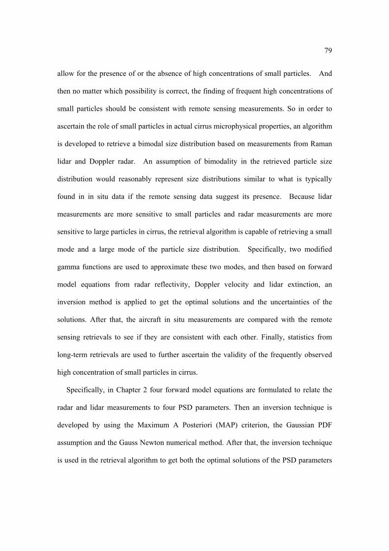
79
allow for the presence of or the absence of high concentrations of small particles. And
then no matter which possibility is correct, the finding of frequent high concentrations of
small particles should be consistent with remote sensing measurements. So in order to
ascertain the role of small particles in actual cirrus microphysical properties, an algorithm
is developed to retrieve a bimodal size distribution based on measurements from Raman
lidar and Doppler radar. An assumption of bimodality in the retrieved particle size
distribution would reasonably represent size distributions similar to what is typically
found in in situ data if the remote sensing data suggest its presence. Because lidar
measurements are more sensitive to small particles and radar measurements are more
sensitive to large particles in cirrus, the retrieval algorithm is capable of retrieving a small
mode and a large mode of the particle size distribution. Specifically, two modified
gamma functions are used to approximate these two modes, and then based on forward
model equations from radar reflectivity, Doppler velocity and lidar extinction, an
inversion method is applied to get the optimal solutions and the uncertainties of the
solutions. After that, the aircraft in situ measurements are compared with the remote
sensing retrievals to see if they are consistent with each other. Finally, statistics from
long-term retrievals are used to further ascertain the validity of the frequently observed
high concentration of small particles in cirrus.
Specifically, in Chapter 2 four forward model equations are formulated to relate the
radar and lidar measurements to four PSD parameters. Then an inversion technique is
developed by using the Maximum A Posteriori (MAP) criterion, the Gaussian PDF
assumption and the Gauss Newton numerical method. After that, the inversion technique
is used in the retrieval algorithm to get both the optimal solutions of the PSD parameters

80
and their uncertainties. For the optimal solutions, the algorithm's ability to reach an
optimal estimation of the PSD parameters is tested, and it is shown that the first guesses
of the PSD parameters should be carefully chosen because of the nonlinearity of this
inverse problem. For the uncertainty estimation, all possible sources of estimation error
are examined, and the two biggest error sources, the model parameter error and the
measurement error, are quantified by using the inversion technique. A sensitivity study is
performed to show the sensitivity of the retrieval error to the model parameter error and
the measurement error, and it is shown that the retrieval error is more sensitive to the
empirically derived power law model parameter error than to the measurement error.
In Chapter 3, a statistical method is first introduced to minimize the time and spatial
differences in the aircraft in situ measurements and the ground-based remote sensing
measurements. And then the in situ measurements, including the PSD data and the IWC
data from 2000 Spring cloud IOP, are used to compare with the retrieval results from
Doppler radar and Raman lidar data. The PSD in situ data from the 2DC for large
particles agree well with that of the retrieval results, but for small particles, the number
concentrations from the FSSP are much higher (by approximately a factor of 10) than that
of the retrievals, and also lie well beyond the retrieval uncertainties. The effect of ice
crystal shattering on the FSSP measurements is considered as a possible reason for this
inconsistency with the remote sensing retrievals.
Finally the bimodality statistics and the statistics of cirrus cloud microphysical
properties are derived by applying the retrieval algorithm to long-term cirrus events. The
data set used amounts to 313 hours of cirrus events collected over the SGP site during
2000. The PDFs of the IWC, the effective radius, and the number concentration are

81
examined for cirrus with different temperatures. We find that bimodality in the PSD is a
significant feature of many cirrus particle size distributions. This is especially true at
warmer cirrus temperatures in the upper half of the cirrus layer where new nucleation
events occur in the presence of larger particles sedimenting from high levels. The
bimodality of the particle size distribution is often prominent enough that an assumption
of a single mode distribution function in remote sensing retrievals would be unable to
simultaneously represent the number concentration, extinction, and IWC. Importantly, we
find unequivocally that the occurrence frequencies of the total number concentrations
larger than 1 cm-3 are less than 1% of all size distributions examined.
In sum, in this study a retrieval algorithm that is designed to retrieve high
concentrations of small particles is developed. The biggest sources of retrieval error are
found and quantified. The small mode concentration retrievals from ground-based radar
and lidar measurements are much lower than those from the aircraft in situ measurements
from the FSSP. Statistics from long-term remote sensing retrievals show that
concentrations in excess of 1 cm-3 are extraordinarily rare, which is also inconsistent with
the frequently observed high concentrations of small particles from aircraft in situ data.
The presence of shattering artifacts in the aircraft in situ data may be the prime reason for
the high concentrations of small particles from in situ data. However, the conclusion of
this study is that high concentrations of small particles from aircraft data (about 1 cm-3
and larger) are inconsistent with any reasonable interpretation of the Doppler radar and
Raman lidar data collected at the SGP site. So it is suggested that previous conclusions
drawn from aircraft in situ data that were not carefully filtered for shattering artifacts
need to be reconsidered.

APPENDIX A
SINGLE MODE RETRIEVAL ALGORITHM If calculated lidar extinction from large mode PSD is greater than the total extinction
from Raman lidar, it suggests another small mode PSD is not necessary, and in this case,
an algorithm that uses radar reflectivity, Doppler velocity and lidar extinction is
performed to retrieve one single mode PSD.
In this single mode radar-lidar algorithm, one modified gamma function, which is
expressed in Equation (A1), is used to represent the PSD.
( ) ( ) exp( )g
g g
D DDN D AD D
α −= − (A1)
The three parameters of the gamma function are included in the vector x:
[ , , ]gA D α=x (A2)
The measurements are included in the vector d:
[ , , ]e dq extZ V β=d (A3)

83
The empirically derived model parameters are included in the vector m:
[ , , , ]m m a aa b a b=m (A4)
Using the same assumptions in the bimodal PSD algorithm, the forward model
equations are expressed in the following:
7 ( 7)zbe z g zZ Aea D bα+= Γ + + (A5)
( 7)( 7)
vb z vdq v g
z
b bV a Db
αα
Γ + + +=
Γ + + (A6)
12 ( 1)abext a g aAea D bβ α+= Γ + + (A7)
The Jacobian matrices that represent the sensitivity to the vector x and the vector m
are expressed in Equation (A8) and (A9).
e e e
g
dq dq dq
g
ext ext ext
g
Z Z ZA D
V V VA D
A D
α
α
β β βα
⎡ ⎤∂ ∂ ∂⎢ ⎥∂ ∂ ∂⎢ ⎥⎢ ⎥∂ ∂ ∂∂ ⎢ ⎥= =
∂ ∂ ∂ ∂⎢ ⎥⎢ ⎥∂ ∂ ∂⎢ ⎥⎢ ⎥∂ ∂ ∂⎣ ⎦
xFKx (A8)
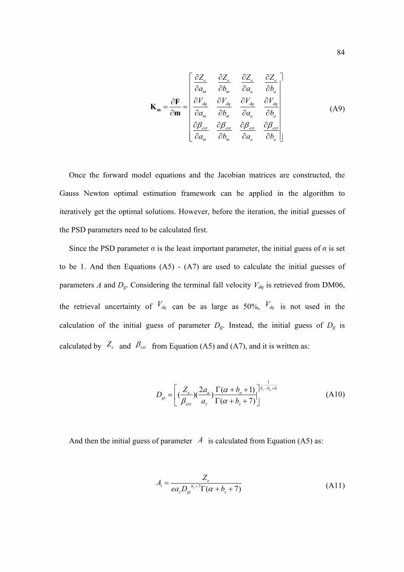
84
e e e e
m m a a
dq dq dq dq
m m a a
ext ext ext ext
m m a a
Z Z Z Za b a bV V V Va b a b
a b a bβ β β β
∂ ∂ ∂ ∂⎡ ⎤⎢ ⎥∂ ∂ ∂ ∂⎢ ⎥⎢ ⎥∂ ∂ ∂ ∂∂
= = ⎢ ⎥∂ ∂ ∂ ∂ ∂⎢ ⎥⎢ ⎥∂ ∂ ∂ ∂⎢ ⎥∂ ∂ ∂ ∂⎢ ⎥⎣ ⎦
mFKm
(A9)
Once the forward model equations and the Jacobian matrices are constructed, the
Gauss Newton optimal estimation framework can be applied in the algorithm to
iteratively get the optimal solutions. However, before the iteration, the initial guesses of
the PSD parameters need to be calculated first.
Since the PSD parameter α is the least important parameter, the initial guess of α is set
to be 1. And then Equations (A5) - (A7) are used to calculate the initial guesses of
parameters A and Dg. Considering the terminal fall velocity Vdq is retrieved from DM06,
the retrieval uncertainty of dqV can be as large as 50%, dqV is not used in the
calculation of the initial guess of parameter Dg. Instead, the initial guess of Dg is
calculated by eZ and extβ from Equation (A5) and (A7), and it is written as:
162 ( 1)( )( )
( 7)z ab b
e a agi
ext z z
Z a bDa b
αβ α
− +⎡ ⎤Γ + += ⎢ ⎥Γ + +⎣ ⎦
(A10)
And then the initial guess of parameter A is calculated from Equation (A5) as:
7 ( 7)z
ei b
z gi z
ZAea D bα+=
Γ + + (A11)
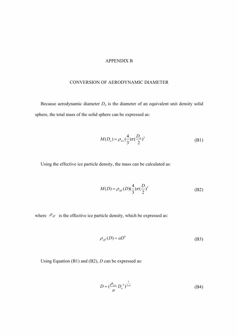
APPENDIX B
CONVERSION OF AERODYNAMIC DIAMETER
Because aerodynamic diameter Da is the diameter of an equivalent unit density solid
sphere, the total mass of the solid sphere can be expressed as:
34( ) ( ) ( )3 2
aa ice
DM D ρ π= (B1)
Using the effective ice particle density, the mass can be calculated as:
34( ) ( )( ) ( )3 2eff
DM D Dρ π= (B2)
where effρ is the effective ice particle density, which be expressed as:
( ) beff D aDρ = (B3)
Using Equation (B1) and (B2), D can be expressed as:
13 3( )ice b
aD Daρ += (B4)
REFERENCES
Arnott, W.P., Y. Dong, and J. Hallett, 1994: Role of small ice crystals in radiative properties of cirrus: A case study, FIRE II, November 22, 1991. Journal of Geophysical Research, 99, 1371-1381. Ansman, A., M. Riebesell, and C. Weitkamp, 1990: Measurement of atmospheric aerosol extinction profiles with a Raman lidar. Optics Letters, 15, 746-748. Aydin, K., and T. M. Walsh, 1999: Millimeter wave scattering from spatial and planar bullet rosettes. IEEE Transaction on Geoscience and Remote Sensing, 37, 1138-1150. Clothiaux, E. E., K. P. Moran, B. E. Martner, T. P. Ackerman, G. G. Mace, T. Uttal, J. H. Mather, M. A. Miller, and D. J. Rodriguez, 1999: The Atmospheric Radiation Measurement Program cloud radars: Operational modes. Journal of Atmospheric Oceanic Technology, 16, 819-827. Comstock, J.M., R.F. Lin, D.O. Starr, and P. Yang, 2008: Understanding ice supersaturation, particle growth, and number concentration in cirrus clouds. Journal of Geophysical Research, 113, D23211. Petty, D., J. Comstock, and D. Tuner, 2006: Cirrus extinction and lidar ratio derived from Raman lidar measurements at the Atmospheric Radiation Measurement Program southern site. Sixteenth ARM Science Team Meeting Proceedings, Albuquerque, NM, 1-8. Deng, M., and G. G. Mace, 2006: Cirrus microphysical properties and air motion statistics using cloud radar Doppler moments: Part I: algorithm description. Journal of Applied Meteorology and Climatology, 45, 1690-1709. Deng, M., and G. G. Mace, 2008: Cirrus microphysical properties and air motion statistics using cloud radar Doppler moments. Part II: Climatology. Journal of Applied Meteorology and Climatology, 47, 3221-3235. Donovan, D. P., 2003: Ice-cloud effective particle size parameterizations based on combined lidar, radar reflectivity, and mean Doppler velocity measurements. Journal of Geophysical Research, 108, 4573-4591. Donovan, D. P., M. Quante, I. Schimme, and A. Macke, 2004: Use of equivalent spheres to model the relation between radar reflectivity and optical extinction of ice cloud particles. Applied Optics, 43, 4929-4940.

87
Doviak, R. J., and D. S. Zrnic, 1984: Doppler Radar and Weather Observations. Academic Press, 458 pp. Field, P. R., R. Wood, P.R. Brown, P.H. Kaye, E. Hirst, R. Greenaway, and J.A. Smith, 2003: Ice particle Interarrival times measured with a fast FSSP. Journal of Atmospheric and Oceanic Technology, 20, 249-261. Gayet, J. F., and A. Minikin, 2002: Quantitative measurement of the microphysical and optical properties of cirrus clouds with four different in situ probes: evidence of small ice crystals. Geophysical Research Letters, 29, 2230. Goldsmith, J., F. H. Blair, S. E. Bisson, and D. Turner, 1998: Turn-key Raman lidar for profiling atmospheric water vapor, clouds, and aerosols. Applied Optics, 37, 4979-4990. Gossard E. E., and R. G. Strauch, 1994: Measurement of cloud droplet size spectra by Doppler radar. Journal of Atmospheric Oceanic Technology, 11, 712-726. Heymsfield, A. J., and C.M.R. Platt, 1984: A parameterization of the particle size spectrum of ice clouds in terms of ambient temperature and the ice water content. Journal of the Atmospheric Sciences, 41, 846-855. Heymsfield, A. J., and J. Iaquinta, 2000: Cirrus crystal terminal velocities. Journal of the Atmospheric Sciences, 57, 916-938. Heymsfield, A.J., and Coauthors, 2003: A General approach for deriving the properties of cirrus and stratiform ice cloud particles. Journal of the Atmospheric Sciences, 59, 3-29. Heymsfield, A. J., C. G. Schmitt, A. Bansemer, D. Baumgardner, E. M. Weinstock, J. T. Smith, and D. Sayres, 2004: Effective ice particle densities for cold anvil cirrus. Geophysical Research Letters, 31, 2101. Heymsfield, A. J., 2007: On measurements of small ice particles in clouds. Geophysical Research Letters, 34, L23812. Ivanova, D., D.L., Mitchell, A.W. Patrick, and M. Poellot, 2001: A GCM parameterization for bimodal size spectra and ice mass removal rates in midlatitude cirrus clouds. Atmospheric Research, 59, 89-113. Korolev, A., and G.A. Isaac, 2004: Shattering during sampling by OAPs and HVPS. Part I: snow particles. Journal of Atmospheric and Oceanic Technology, 22, 528-542. Lawson, R. P., B. Baker, B. Pilson, and Q. Mo, 2006: In situ observations of the microphysical properties of wave, cirrus, and anvil clouds, Part II: Cirrus Clouds. Journal of the Atmospheric Sciences, 63, 3186-3203. Lewis S., A. Heymsfield, C. Twohy, and M. Poellot, 2001: In situ microphysical

88
measurements of cirrus properties during ARM 2000 IOP. Eleventh ARM Science Team Meeting Proceedings, Atlanta, Georgia, 1-9. Liu, G.S., 2008: A database of microwave single scattering properties for non-spherical ice particles. Bulletin of the American Meteorological Society, 89, 1563-1570. Mace, G. G., T.P. Ackerman, E.E. Clothiaux, and B.A. Albrecht, 1997: A study of composite cirrus morphology using data from a 94-GHz radar and correlations with temperature and large-scale vertical motion, Journal of Geophyscial Research, 102, 13581-13593. Mace, G. G., T. P. Ackerman, P. Minnis, and D. F. Young, 1998: Cirrus layer microphysical properties derived from surface-based millimeter radar and infrared interferometer data. Journal of Geophysical Research, 103, 23207-23216. Mace G. G., A. J. Heymsfield, and M. R. Poellot, 2002: On retrieving the microphysical properties of cirrus clouds using the moments of the millimeter-wavelength Doppler spectrum. Journal of Geophysical Research, 107, 4815-4841. Mace, G. G., E. E. Clothiaux, and T. P. Ackerman, 2001: The composite characteristics of cirrus clouds: Bulk properties revealed by one year of continuous cloud radar data. Journal of Climate, 14, 2185-2203. Matrosov, S. Y., 1997: Variability of microphysical parameters in high-altitude ice clouds: Results of the remote sensing method. Journal of Applied Meteorology, 36, 633-648. Matrosov, S. Y., and Coauthors, 1998: Comparisons of ice cloud parameters obtained by combined remote sensor retrievals and direct methods. Journal of Atmospheric and Oceanic Technology, 15, 184-196. Matrosov, S. Y., and A. J. Heymsfield, 2000: Use of Doppler radar to assess ice cloud particle fall velocity-size relations for remote sensing and climate studies, Journal of Geophysical Research, 105, 22427-22436. Mitchell, D. L., 1996: Use of mass- and area-dimensional power laws for determining precipitation particle terminal velocities. Journal of the Atmospheric Sciences, 53, 1710-1723. Mitchell, D. L., S.K. Chai, Y. Liu, A.J. Heymsfield, and Y. Dong, 1996: Modeling cirrus clouds. Part I: Treatment of bimodal size spectra and case study analysis. Journal of the Atmospheric Sciences, 53, 2952-2966. Nelder, J. A. and R. Mead, 1965: A simplex method for function minimization. Computer Journal, 7, 308-313.

89
Platt, C., and R. Martin, 1997: A parameterization of the visible extinction coefficient of ice clouds in terms of the ice/water content. Journal of the Atmospheric Sciences, 54, 2083-2098. Protat, A., J. Delanoe, D. Bouniol, A.J. Heymsfield, A. Bansemer, and P. Brown, 2007: Evaluation of ice water content retrievals from cloud radar reflectivity and temperature using a large airborne in situ microphysical database. Journal of Applied Meteorology and Climatology, 46, 557-572. Roger, C. D., 2000: Inverse Methods for Atmospheric Sounding: Theory and Practice. World Scientific, 240 pp. Stephens, G. L., 2005: Cloud feedback in the climate system: A critical review. Journal of Climate, 18, 237-273. Turner, D.D., 2004: Raman Lidar Handbook, DOE/ARM TR-038, 29 pp. Twohy, C. H., A.J. Schanot, and W.A. Cooper, 1997: Measurement of condensed water content in liquid and ice clouds using an airborne counterflow virtual impactor. Journal of Atmospheric and Oceanic Technology, 14, 197-202. Twohy, C. H., J.W. Strapp, and M. Wendisch, 2003: Performance of a counterflow virtual impactor in the NASA icing research tunnel. Journal of Atmospheric and Oceanic Technology, 20, 781-790. Wang, Z., and K. Sassen, 2001: Cirrus cloud microphysical property retrieval using lidar and radar measurements, part I: Algorithm description and comparison with in situ data. Journal of Applied Meteorology, 41, 218-227. Wunsch, C., 2006: Discrete Inverse and State Estimation Problems with Geophysical Fluid Applications. Cambridge University Press, 384 pp. Zhdanov, M., 2002: Geophysical Inverse Theory and Regularization Problems. Elsevier Science, 633 pp.