CISC 4631 Data Mining

Lecture 09: • Clustering

Theses slides are based on the slides by • Tan, Steinbach and Kumar (textbook authors)

• Eamonn Koegh (UC Riverside)

• Raymond Mooney (UT Austin)

What is Clustering? Finding groups of objects such that objects in a group will be similar to

one another and different from the objects in other groups

Also called unsupervised learning, sometimes called classification by statisticians and sorting by psychologists and segmentation by people in marketing

Inter-cluster distances are maximized

Intra-cluster distances are

minimized

3 School Employees Simpson's Family Males Females

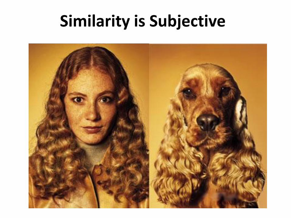
Clustering is subjective

What is a natural grouping among these objects?

4

Similarity is Subjective

5

Intuitions behind desirable

distance measure properties

D(A,B) = D(B,A) Symmetry Otherwise you could claim “Alex looks like Bob, but Bob looks nothing like Alex.”

D(A,A) = 0 Constancy of Self-Similarity Otherwise you could claim “Alex looks more like Bob, than Bob does.”

D(A,B) = 0 IIf A=B Positivity (Separation) Otherwise there are objects in your world that are different, but you cannot tell apart.

D(A,B) D(A,C) + D(B,C) Triangular Inequality Otherwise you could claim “Alex is very like Bob, and Alex is very like Carl, but Bob is very unlike Carl.”

Applications of Cluster Analysis

Understanding

– Group related documents

for browsing, group genes

and proteins that have

similar functionality, group

stocks with similar price

fluctuations, or customers

that have similar buying

habits

Summarization

– Reduce the size of large

data sets

Discovered Clusters Industry Group

1 Applied-Matl-DOWN,Bay-Network-Down,3-COM-DOWN,

Cabletron-Sys-DOWN,CISCO-DOWN,HP-DOWN,

DSC-Comm-DOWN,INTEL-DOWN,LSI-Logic-DOWN,

Micron-Tech-DOWN,Texas-Inst-Down,Tellabs-Inc-Down,

Natl-Semiconduct-DOWN,Oracl-DOWN,SGI-DOWN,

Sun-DOWN

Technology1-DOWN

2 Apple-Comp-DOWN,Autodesk-DOWN,DEC-DOWN,

ADV-Micro-Device-DOWN,Andrew-Corp-DOWN,

Computer-Assoc-DOWN,Circuit-City-DOWN,

Compaq-DOWN, EMC-Corp-DOWN, Gen-Inst-DOWN,

Motorola-DOWN,Microsoft-DOWN,Scientific-Atl-DOWN

Technology2-DOWN

3 Fannie-Mae-DOWN,Fed-Home-Loan-DOWN,

MBNA-Corp-DOWN,Morgan-Stanley-DOWN

Financial-DOWN

4 Baker-Hughes-UP,Dresser-Inds-UP,Halliburton-HLD-UP,

Louisiana-Land-UP,Phillips-Petro-UP,Unocal-UP,

Schlumberger-UP

Oil-UP

Clustering precipitation

in Australia

Notion of a Cluster can be Ambiguous

How many clusters?

Four Clusters Two Clusters

Six Clusters

So tell me how

many clusters do

you see?

Types of Clusterings

A clustering is a set of clusters

Important distinction between hierarchical and partitional sets of clusters

Partitional Clustering – A division data objects into non-overlapping subsets (clusters) such

that each data object is in exactly one subset

Hierarchical clustering – A set of nested clusters organized as a hierarchical tree

Partitional Clustering

Original Points A Partitional Clustering

Hierarchical Clustering

p4

p1 p3

p2

p4p1 p2 p3

Traditional Hierarchical Clustering Traditional Dendrogram

Simpsonian Dendrogram

Other Distinctions Between Sets of Clusters

Exclusive versus non-exclusive – In non-exclusive clusterings points may belong to multiple clusters

– Can represent multiple classes or ‘border’ points

Fuzzy versus non-fuzzy – In fuzzy clustering, a point belongs to every cluster with some weight

between 0 and 1

– Weights must sum to 1

– Probabilistic clustering has similar characteristics

Partial versus complete – In some cases, we only want to cluster some of the data

Types of Clusters

Well-separated clusters

Center-based clusters (our main emphasis)

Contiguous clusters

Density-based clusters

Described by an Objective Function

Types of Clusters: Well-Separated

Well-Separated Clusters: – A cluster is a set of points such that any point in a cluster is closer

(or more similar) to every other point in the cluster than to any point not in the cluster.

3 well-separated clusters

Types of Clusters: Center-Based

Center-based – A cluster is a set of objects such that an object in a cluster is closer

(more similar) to the “center” of a cluster, than to the center of any other cluster

– The center of a cluster is often a centroid, the average of all the points in the cluster (assuming numerical attributes), or a medoid, the most “representative” point of a cluster (used if there are categorical features)

4 center-based clusters

Types of Clusters: Contiguity-Based

Contiguous Cluster (Nearest neighbor or Transitive) – A cluster is a set of points such that a point in a cluster is closer (or

more similar) to one or more other points in the cluster than to any point not in the cluster.

8 contiguous clusters

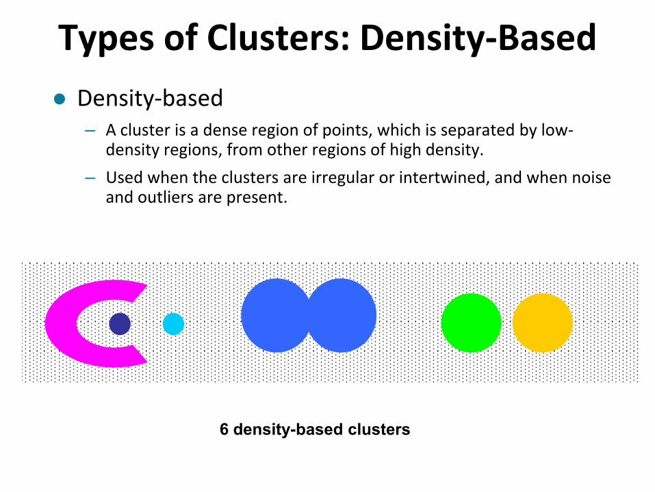
Types of Clusters: Density-Based

Density-based – A cluster is a dense region of points, which is separated by low-

density regions, from other regions of high density.

– Used when the clusters are irregular or intertwined, and when noise and outliers are present.

6 density-based clusters

Types of Clusters: Objective Function

Clusters Defined by an Objective Function

– Finds clusters that minimize or maximize an objective function.

– Enumerate all possible ways of dividing the points into clusters and evaluate the `goodness' of each potential set of clusters by using the given objective function. (NP Hard)

– Example: Sum of squares of distances to cluster center

Clustering Algorithms

K-means and its variants

Hierarchical clustering

Density-based clustering

K-means Clustering

Partitional clustering approach

Each cluster is associated with a centroid (center point)

Each point is assigned to the cluster with the closest centroid

Number of clusters, K, must be specified

The basic algorithm is very simple

– K-means tutorial available from http://maya.cs.depaul.edu/~classes/ect584/WEKA/k-means.html

20

0

1

2

3

4

5

0 1 2 3 4 5

K-means Clustering 1. Ask user how

many clusters they’d like. (e.g. k=3)

2. Randomly guess k cluster Center locations

3. Each datapoint finds out which Center it’s closest to.

4. Each Center finds the centroid of the points it owns…

5. …and jumps there

6. …Repeat until terminated!

21

0

1

2

3

4

5

0 1 2 3 4 5

KK--means Clustering: Step 1means Clustering: Step 1

k1

k2

k3

22

0

1

2

3

4

5

0 1 2 3 4 5

K-means Clustering

k1

k2

k3

23

0

1

2

3

4

5

0 1 2 3 4 5

K-means Clustering

k1

k2

k3

24

0

1

2

3

4

5

0 1 2 3 4 5

K-means Clustering

k1

k2

k3

25

0

1

2

3

4

5

0 1 2 3 4 5

expression in condition 1

exp

ressio

n in

co

nd

itio

n 2

K-means Clustering

k1

k2 k3

K-means Clustering – Details

Initial centroids are often chosen randomly.

– Clusters produced vary from one run to another.

The centroid is (typically) the mean of the points in the cluster

‘Closeness’ is measured by Euclidean distance, correlation, etc.

K-means will converge for common similarity measures mentioned above.

Most of the convergence happens in the first few iterations.

– Often the stopping condition is changed to ‘Until relatively few points change clusters’

Evaluating K-means Clusters

Most common measure is Sum of Squared Error (SSE) – For each point, the error is the distance to the nearest

cluster

– To get SSE, we square these errors and sum them.

– We can show that to minimize SSE the best update strategy is to use the center of the cluster.

– Given two clusters, we can choose the one with the smallest error

– One easy way to reduce SSE is to increase K, the number of clusters A good clustering with smaller K can have a lower SSE than a poor clustering with higher K

Two different K-means Clusterings

-2 -1.5 -1 -0.5 0 0.5 1 1.5 2

0

0.5

1

1.5

2

2.5

3

x

y

-2 -1.5 -1 -0.5 0 0.5 1 1.5 2

0

0.5

1

1.5

2

2.5

3

x

y

Sub-optimal Clustering

-2 -1.5 -1 -0.5 0 0.5 1 1.5 2

0

0.5

1

1.5

2

2.5

3

x

y

Optimal Clustering

Original Points

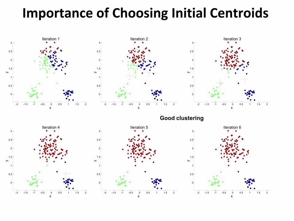
Importance of Choosing Initial Centroids

-2 -1.5 -1 -0.5 0 0.5 1 1.5 2

0

0.5

1

1.5

2

2.5

3

x

y

Iteration 1

-2 -1.5 -1 -0.5 0 0.5 1 1.5 2

0

0.5

1

1.5

2

2.5

3

x

y

Iteration 2

-2 -1.5 -1 -0.5 0 0.5 1 1.5 2

0

0.5

1

1.5

2

2.5

3

x

y

Iteration 3

-2 -1.5 -1 -0.5 0 0.5 1 1.5 2

0

0.5

1

1.5

2

2.5

3

x

y

Iteration 4

-2 -1.5 -1 -0.5 0 0.5 1 1.5 2

0

0.5

1

1.5

2

2.5

3

x

y

Iteration 5

-2 -1.5 -1 -0.5 0 0.5 1 1.5 2

0

0.5

1

1.5

2

2.5

3

x

y

Iteration 6

If you happen to choose good initial centroids, then you will

get this after 6 iterations

Importance of Choosing Initial Centroids

-2 -1.5 -1 -0.5 0 0.5 1 1.5 2

0

0.5

1

1.5

2

2.5

3

x

y

Iteration 1

-2 -1.5 -1 -0.5 0 0.5 1 1.5 2

0

0.5

1

1.5

2

2.5

3

x

y

Iteration 2

-2 -1.5 -1 -0.5 0 0.5 1 1.5 2

0

0.5

1

1.5

2

2.5

3

x

y

Iteration 3

-2 -1.5 -1 -0.5 0 0.5 1 1.5 2

0

0.5

1

1.5

2

2.5

3

x

y

Iteration 4

-2 -1.5 -1 -0.5 0 0.5 1 1.5 2

0

0.5

1

1.5

2

2.5

3

x

y

Iteration 5

-2 -1.5 -1 -0.5 0 0.5 1 1.5 2

0

0.5

1

1.5

2

2.5

3

x

y

Iteration 6

Good clustering

Importance of Choosing Initial Centroids …

-2 -1.5 -1 -0.5 0 0.5 1 1.5 2

0

0.5

1

1.5

2

2.5

3

x

y

Iteration 1

-2 -1.5 -1 -0.5 0 0.5 1 1.5 2

0

0.5

1

1.5

2

2.5

3

x

y

Iteration 2

-2 -1.5 -1 -0.5 0 0.5 1 1.5 2

0

0.5

1

1.5

2

2.5

3

x

y

Iteration 3

-2 -1.5 -1 -0.5 0 0.5 1 1.5 2

0

0.5

1

1.5

2

2.5

3

x

y

Iteration 4

-2 -1.5 -1 -0.5 0 0.5 1 1.5 2

0

0.5

1

1.5

2

2.5

3

xy

Iteration 5

Bad

Clustering

10 Clusters Example

0 5 10 15 20

-6

-4

-2

0

2

4

6

8

x

y

Iteration 1

0 5 10 15 20

-6

-4

-2

0

2

4

6

8

x

y

Iteration 2

0 5 10 15 20

-6

-4

-2

0

2

4

6

8

x

y

Iteration 3

0 5 10 15 20

-6

-4

-2

0

2

4

6

8

x

y

Iteration 4

Starting with two initial centroids in one cluster of each pair of clusters

10 Clusters Example

Starting with some pairs of clusters having three initial centroids, while other have only one.

0 5 10 15 20

-6

-4

-2

0

2

4

6

8

x

yIteration 1

0 5 10 15 20

-6

-4

-2

0

2

4

6

8

x

y

Iteration 2

0 5 10 15 20

-6

-4

-2

0

2

4

6

8

x

y

Iteration 3

0 5 10 15 20

-6

-4

-2

0

2

4

6

8

x

y

Iteration 4

Pre-processing and Post-processing

Pre-processing

– Normalize the data

– Eliminate outliers

Post-processing

– Eliminate small clusters that may represent outliers

– Split ‘loose’ clusters, i.e., clusters with relatively high SSE

– Merge clusters that are ‘close’ and that have relatively low SSE

Limitations of K-means

K-means has problems when clusters are of differing

– Sizes (biased toward the larger clusters)

– Densities

– Non-globular shapes

K-means has problems when the data contains outliers.

Limitations of K-means: Differing Sizes

Original Points K-means (3 Clusters)

Limitations of K-means: Differing Density

Original Points K-means (3 Clusters)

Limitations of K-means: Non-globular Shapes

Original Points K-means (2 Clusters)

Overcoming K-means Limitations

Original Points K-means Clusters

One solution is to use many clusters.

Find parts of clusters, but need to put together.

Overcoming K-means Limitations

Original Points K-means Clusters

Overcoming K-means Limitations

Original Points K-means Clusters

Hierarchical Clustering

Produces a set of nested clusters organized as a hierarchical tree

Can be visualized as a dendrogram

– A tree like diagram that records the sequences of merges or splits

1 3 2 5 4 60

0.05

0.1

0.15

0.2

1

2

3

4

5

6

1

23 4

5

43 ANGUILLA AUSTRALIA

St. Helena &

Dependencies

South Georgia &

South Sandwich

Islands U.K.

Serbia &

Montenegro

(Yugoslavia) FRANCE NIGER INDIA IRELAND BRAZIL

Hierarchal clustering can sometimes show

patterns that are meaningless or spurious • For example, in this clustering, the tight grouping of Australia, Anguilla,

St. Helena etc is meaningful, since all these countries are former UK

colonies.

• However the tight grouping of Niger and India is completely spurious,

there is no connection between the two.

44 ANGUILLA AUSTRALIA

St. Helena &

Dependencies

South Georgia &

South Sandwich

Islands U.K.

Serbia &

Montenegro

(Yugoslavia) FRANCE NIGER INDIA IRELAND BRAZIL

• The flag of Niger is orange over white over green, with an orange disc on the

central white stripe, symbolizing the sun. The orange stands the Sahara desert,

which borders Niger to the north. Green stands for the grassy plains of the south

and west and for the River Niger which sustains them. It also stands for fraternity

and hope. White generally symbolizes purity and hope.

• The Indian flag is a horizontal tricolor in equal proportion of deep saffron on the

top, white in the middle and dark green at the bottom. In the center of the white

band, there is a wheel in navy blue to indicate the Dharma Chakra, the wheel of

law in the Sarnath Lion Capital. This center symbol or the 'CHAKRA' is a symbol

dating back to 2nd century BC. The saffron stands for courage and sacrifice; the

white, for purity and truth; the green for growth and auspiciousness.

45

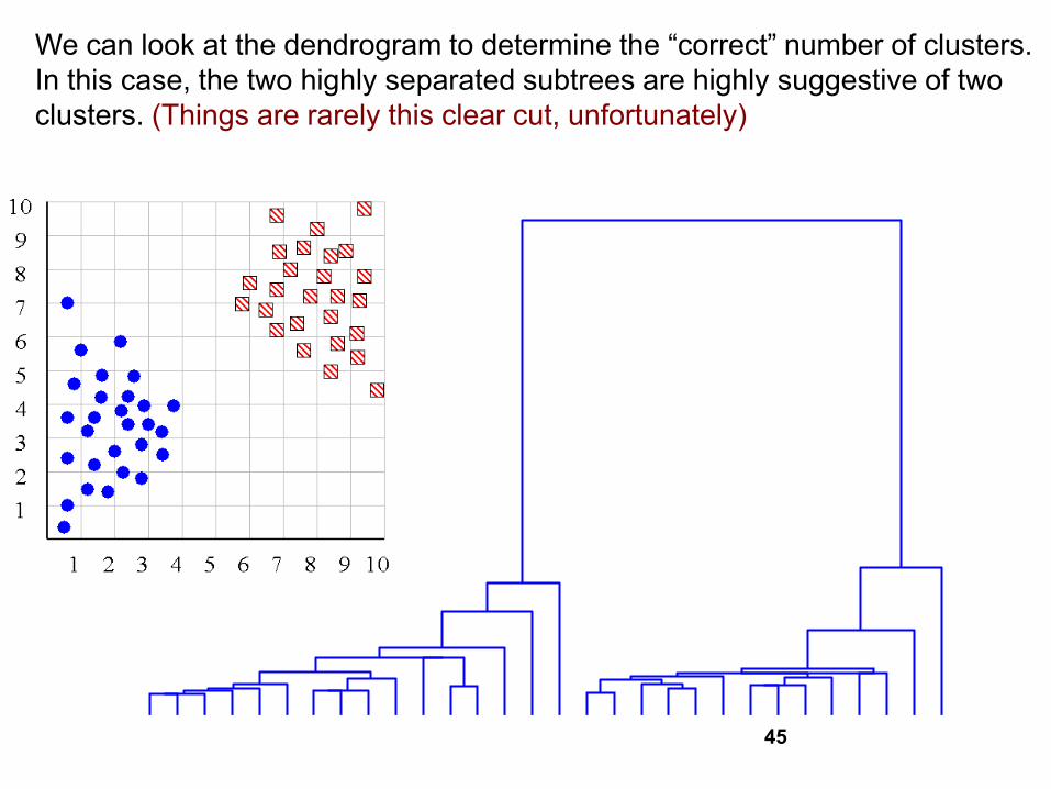
We can look at the dendrogram to determine the “correct” number of clusters.

In this case, the two highly separated subtrees are highly suggestive of two

clusters. (Things are rarely this clear cut, unfortunately)

46

Outlier

One potential use of a dendrogram is to detect outliers

The single isolated branch is suggestive of a data

point that is very different to all others

47

Hierarchical Clustering

Build a tree-based hierarchical taxonomy (dendrogram) from a set of

unlabeled examples.

Recursive application of a standard clustering algorithm can produce

a hierarchical clustering.

animal

vertebrate

fish reptile amphib. mammal worm insect crustacean

invertebrate

Strengths of Hierarchical Clustering

Do not have to assume any particular number of clusters – Any desired number of clusters can be obtained by

‘cutting’ the dendogram at the proper level

They may correspond to meaningful taxonomies – Example in biological sciences (e.g., animal kingdom,

phylogeny reconstruction, …)

49 (Bovine:0.69395, (Spider Monkey 0.390, (Gibbon:0.36079,(Orang:0.33636,(Gorilla:0.17147,(Chimp:0.19268,

Human:0.11927):0.08386):0.06124):0.15057):0.54939);

There is only one dataset that can be

perfectly clustered using a hierarchy…

Hierarchical Clustering

Two main types of hierarchical clustering

– Agglomerative:

Start with the points as individual clusters

At each step, merge the closest pair of clusters until only one cluster (or k clusters) left

– Divisive:

Start with one, all-inclusive cluster

At each step, split a cluster until each cluster contains a point (or there are k clusters)

Agglomerative is most common

Starting Situation

Start with clusters of individual points

...p1 p2 p3 p4 p9 p10 p11 p12

Intermediate Situation

After some merging steps, we have some clusters

C1

C4

C2 C5

C3

...p1 p2 p3 p4 p9 p10 p11 p12

Intermediate Situation

We want to merge the two closest clusters (C2 and C5)

C1

C4

C2 C5

C3

...p1 p2 p3 p4 p9 p10 p11 p12

How to Define Inter-Cluster Similarity

p1

p3

p5

p4

p2

p1 p2 p3 p4 p5 . . .

.

.

.

Similarity?

MIN

MAX

Group Average

Distance Between Centroids

Other methods driven by an objective

function

– Ward’s Method uses squared error

Proximity Matrix

How to Define Inter-Cluster Similarity

p1

p3

p5

p4

p2

p1 p2 p3 p4 p5 . . .

.

.

. Proximity Matrix

MIN

MAX

Group Average

Distance Between Centroids

Other methods driven by an objective

function

– Ward’s Method uses squared error

How to Define Inter-Cluster Similarity

p1

p3

p5

p4

p2

p1 p2 p3 p4 p5 . . .

.

.

. Proximity Matrix

MIN

MAX

Group Average

Distance Between Centroids

Other methods driven by an objective

function

– Ward’s Method uses squared error

How to Define Inter-Cluster Similarity

p1

p3

p5

p4

p2

p1 p2 p3 p4 p5 . . .

.

.

. Proximity Matrix

MIN

MAX

Group Average

Distance Between Centroids

Other methods driven by an objective

function

– Ward’s Method uses squared error

How to Define Inter-Cluster Similarity

p1

p3

p5

p4

p2

p1 p2 p3 p4 p5 . . .

.

.

. Proximity Matrix

MIN

MAX

Group Average

Distance Between Centroids

Hierarchical Clustering: MIN

Nested Clusters Dendrogram

1

2

3

4

5

6

1

2

3

4

5

3 6 2 5 4 10

0.05

0.1

0.15

0.2

Hierarchical Clustering: MAX

Nested Clusters Dendrogram

3 6 4 1 2 50

0.05

0.1

0.15

0.2

0.25

0.3

0.35

0.4

1

2

3

4

5

6

1

2 5

3

4

Hierarchical Clustering: Problems and Limitations

Once a decision is made to combine two clusters, it cannot be undone

No objective function is directly minimized

Different schemes have problems with one or more of the following:

– Sensitivity to noise and outliers

– Difficulty handling different sized clusters and convex shapes

– Breaking large clusters

DBSCAN

DBSCAN is a density-based algorithm. – Density = number of points within a specified radius (Eps)

– A point is a core point if it has more than a specified number of points (MinPts) within Eps

These are points that are at the interior of a cluster

– A border point has fewer than MinPts within Eps, but is in the neighborhood of a core point

– A noise point is any point that is not a core point or a border point.

DBSCAN: Core, Border, and Noise Points

DBSCAN: Core, Border and Noise Points

Original Points Point types: core,

border and noise

Eps = 10, MinPts = 4

When DBSCAN Works Well

Original Points Clusters

• Resistant to Noise

• Can handle clusters of different shapes and sizes

When DBSCAN Does NOT Work Well

Original Points

(MinPts=4, Eps=9.75).

(MinPts=4, Eps=9.92)

• Varying densities

Cluster Validity

For supervised classification we have a variety of measures to evaluate how good our model is

– Accuracy, precision, recall

For cluster analysis, the analogous question is how to evaluate the “goodness” of the resulting clusters?

But “clusters are in the eye of the beholder”!

Then why do we want to evaluate them? – To avoid finding patterns in noise

– To compare clustering algorithms

– To compare two sets of clusters

– To compare two clusters

Clusters found in Random Data

0 0.2 0.4 0.6 0.8 10

0.1

0.2

0.3

0.4

0.5

0.6

0.7

0.8

0.9

1

x

y

Random

Points

0 0.2 0.4 0.6 0.8 10

0.1

0.2

0.3

0.4

0.5

0.6

0.7

0.8

0.9

1

x

y

K-means

0 0.2 0.4 0.6 0.8 10

0.1

0.2

0.3

0.4

0.5

0.6

0.7

0.8

0.9

1

x

y

DBSCAN

0 0.2 0.4 0.6 0.8 10

0.1

0.2

0.3

0.4

0.5

0.6

0.7

0.8

0.9

1

x

y

Complete

Link

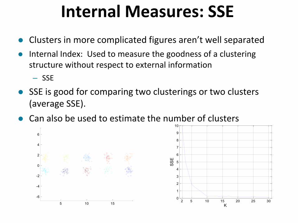
Clusters in more complicated figures aren’t well separated

Internal Index: Used to measure the goodness of a clustering structure without respect to external information

– SSE

SSE is good for comparing two clusterings or two clusters (average SSE).

Can also be used to estimate the number of clusters

Internal Measures: SSE

2 5 10 15 20 25 300

1

2

3

4

5

6

7

8

9

10

K

SS

E

5 10 15

-6

-4

-2

0

2

4

6

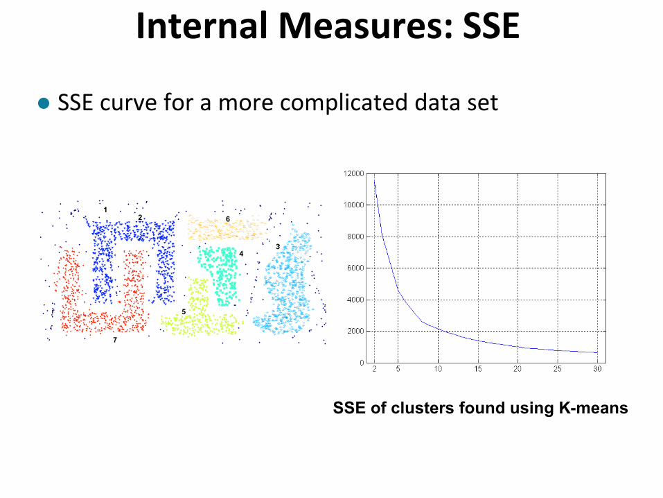
Internal Measures: SSE

SSE curve for a more complicated data set

1 2

3

5

6

4

7

SSE of clusters found using K-means

“The validation of clustering structures is the most difficult and frustrating part of cluster analysis.

Without a strong effort in this direction, cluster analysis will remain a black art accessible only to those true believers who have experience and great courage.”

Algorithms for Clustering Data, Jain and Dubes

Final Comment on Cluster Validity

For some info on clustering with WEKA, follow this link: – http://www.ibm.com/developerworks/opensource/library/os-weka2/index.html

Clustering with WEKA