ETHIOPIAN DEVELOPMENT RESEARCH INSTITUTE

Cities and agricultural transformation in Ethiopia

PRELIMINARY RESULTS

Joachim Vandercasteelen, Seneshaw Tamru, Bart Minten and Johan Swinnen

IFPRI ESSP

EDRIAddis Ababa, Ethiopia

1

2

1. Introduction

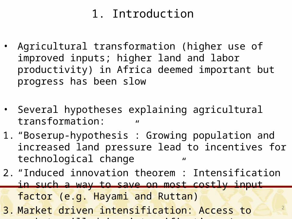
• Agricultural transformation (higher use of improved inputs; higher land and labor productivity) in Africa deemed important but progress has been slow

• Several hypotheses explaining agricultural transformation:1. “Boserup-hypothesis”: Growing population and increased land

pressure lead to incentives for technological change 2. “Induced innovation theorem”: Intensification in such a way to save

on most costly input factor (e.g. Hayami and Ruttan)3. Market driven intensification: Access to markets will drive

intensification (e.g. Pingali and Binswanger; Reardon and Timmer)

3

1. Introduction • Urbanization important new factor for transformation in Africa:- People living in cities in Sub-Saharan Africa increased by 160%

between 1990-2014- Urban population in Africa expected to triple by 2050 (1.3 billion

people)• Urbanization important economic impacts, associated with

structural transformation:1. Shift from low productivity agriculture to more productive non-

agriculture2. Agglomeration effects – economies of scale3. Employment and labor markets develop4. Spill-overs on rural areas (remittances, non-farm income)

4

1. Introduction • Important effects on agriculture and food markets:1. Urban residents often do not grow own food; More commercial

agricultural rural-urban flows2. Urban residents have different diets and consume more high-value

crops3. Urban residents are often richer and are willing to pay more, leading

to higher consumption of ready-to-eat and processed foods and demand for food safety and quality.

• Most of the literature focused of effect of urbanization on changes in crops (von Thunen) or off-farm employment (e.g. Fafchamps and Shilpi)

• Relatively little evidence on impacts on staple crops, that most of the rural population makes a living from

5

1. Introduction

• Look at the case of Ethiopia and at teff (most important crop area-wise)

• Question: “How does proximity to urban centers affect farmers’ agricultural production environment and practices?”

• Important changes in Ethiopia in this area1996/1997 2010/2011

6

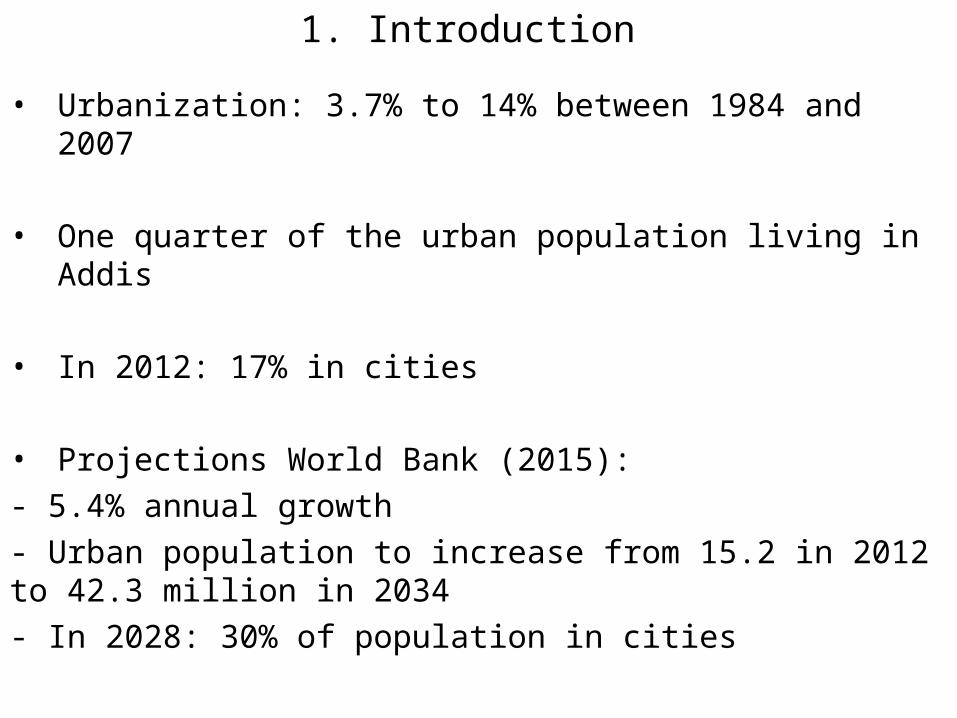
1. Introduction

• Urbanization: 3.7% to 14% between 1984 and 2007

• One quarter of the urban population living in Addis

• In 2012: 17% in cities

• Projections World Bank (2015):- 5.4% annual growth- Urban population to increase from 15.2 in 2012 to 42.3 million in 2034- In 2028: 30% of population in cities

7

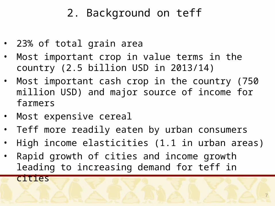
2. Background on teff

• 23% of total grain area• Most important crop in value terms in the country (2.5 billion USD in

2013/14)• Most important cash crop in the country (750 million USD) and

major source of income for farmers• Most expensive cereal• Teff more readily eaten by urban consumers• High income elasticities (1.1 in urban areas)• Rapid growth of cities and income growth leading to increasing

demand for teff in cities

8

3. Methodology (a) Sampling and data• Stratified random sample in 2012• 1,200 farmers in five major teff production zones. These five zones

represent 38% of national teff area and 42% of the commercial surplus.

• Urban proximity main independent variable: Measured by transportation costs that farmers face when selling teff in Addis (ETB/quintal)

• Two components:1/ Cost of transporting teff from the farm to the market center2/ Cost of transporting teff from the market center to the Addis wholesale market by truck

9

3. Methodology

10

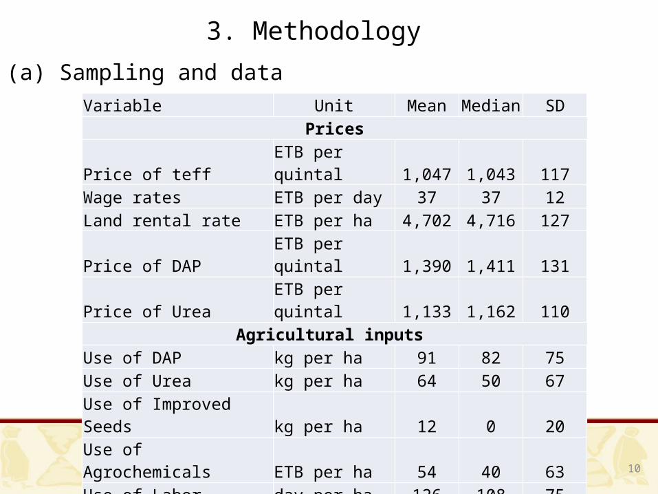
3. Methodology (a) Sampling and data

Variable Unit Mean Median SDPrices

Price of teff ETB per quintal 1,047 1,043 117Wage rates ETB per day 37 37 12Land rental rate ETB per ha 4,702 4,716 127Price of DAP ETB per quintal 1,390 1,411 131Price of Urea ETB per quintal 1,133 1,162 110

Agricultural inputs Use of DAP kg per ha 91 82 75Use of Urea kg per ha 64 50 67Use of Improved Seeds kg per ha 12 0 20Use of Agrochemicals ETB per ha 54 40 63Use of Labor day per ha 126 108 75

Intensification outcomesTeff Land Productivity kg per ha 1,071 978 600Teff Labor Productivity kg per day 10 9 6Teff Input Cost ETB per ha 3,277 2,879 1,859Teff Non-labor Input Cost ETB per ha 2,514 2,243 1,560Teff Profits ETB per ha 7,384 6,228 5,880

11

3. Methodology (b) Empirical strategy • Two models: 1/ reduced form; 2/ less parsimonious• Urban proximity (d); Prices (p); Agricultural inputs and indices (q);

Intensification outcome (y)• Estimation using Seemingly Unrelated Regression (SUR) set-up and

bootstrapped standard errors• Differentiate direct (due to improved information, transaction costs,

institution) and indirect effect (due to changing input and output prices) of urban proximity; total effect is combination of both

(1)

12

3. Methodology (b) Empirical strategy • Controls: 1. Farm characteristics (age, gender, ethnicity, and education of

household head)2. Household assets and household size3. Agro-ecological conditions (altitude, share brown/black soil, share of

flat – versus sloped – land)4. Population pressure:- Often used GIS measures of rural population density (however, not

easily available; issue with soil quality/geography measure; strong interpolation assumptions)

- Follow Headey et al. (2014) and use average farm size at the kebele level (collected from the Bureau of Agriculture)

13

3. Methodology (c) Estimation issues • Unobserved heterogeneity; cities do not develop randomly over

space; likely to emerge in areas with favourable agro-ecological condition and potential; Settlement in hinterland also not random; Complicated…

• Two tests: 1/ Is there heterogeneity of land over space (give all some inputs)? 2/ Do unobserved fixed abilities of farmers vary over space?

Observed Yield (kg/ha)

Adjusted Yield (kg/ha)

Farming Ability (.)

Transportation Cost (ETB/quintal)

-2.232*** -0.975 -0.001

(0.700) (0.702) (0.001)

Constant 1,2889*** 1,181*** 0.067

(70) (65) (0.110)Observations 2,791 2,786 2,786R-squared 0.010 0.002 0.003

14

4. Non-parametric regressions - Advantage: No functional form specified in advance

- Local polynomial smoothing estimates

- Do for the four major outcomes:1. Prices2. Input3. Input indices4. Intensification

15

4. Non-parametric regressions - prices

16

4. Non-parametric regressions – use of inputs

17

4. Non-parametric regressions – input ratios

18

4. Non-parametric regressions – intensification

19

5. Multi-variate regression results – prices

Prices log of teff prices (ETB/quintal)

log of wage (ETB/day)

log of land rent

(ETB/ha)

log of DAP price

(ETB/qtl)

log of urea price

(ETB/qtl)REDUCED FORM MODEL

Transportation Cost (ETB/quintal)

-0.86*** -3.06*** -0.18*** -0.02 -0.01(0.22) (0.89) (0.03) (0.26) (0.30)

Constant 7,021.8*** 3,839.1*** 8,471.0*** 7,233.3*** 7,028.7***(18.49) (86.08) (2.89) (23.77) (26.88)

R-squared 0.066 0.106 0.050 0.000 0.000 LESS PARSIMONIOUS MODEL

Transportation Cost (ETB/quintal)

-0.55*** -2.48** -0.13*** 0.31 0.46(0.20) (1.14) (0.04) (0.29) (0.35)

Farm Size at village level (ha)

2.55 52.54 1.78 39.41*** 40.43***(7.95) (47.64) (1.52) (14.36) (14.93)

Constant 6,875.39*** 3,955.94*** 8,480.4*** 7,144.6*** 6,936.6***(65.38) (401.56) (10.94) (113.26) (99.33)

R-squared 0.126 0.161 0.282 0.202 0.180

20

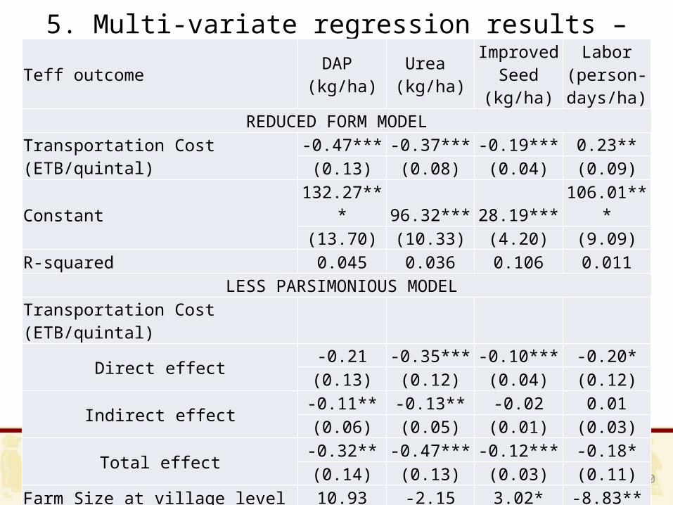
5. Multi-variate regression results – input use Teff outcome DAP

(kg/ha)Urea

(kg/ha)Improved

Seed (kg/ha)

Labor (person-days/ha)

REDUCED FORM MODEL

Transportation Cost (ETB/quintal) -0.47*** -0.37*** -0.19*** 0.23**(0.13) (0.08) (0.04) (0.09)

Constant 132.27*** 96.32*** 28.19*** 106.01***(13.70) (10.33) (4.20) (9.09)

R-squared 0.045 0.036 0.106 0.011 LESS PARSIMONIOUS MODEL

Transportation Cost (ETB/quintal)

Direct effect -0.21 -0.35*** -0.10*** -0.20*(0.13) (0.12) (0.04) (0.12)

Indirect effect -0.11** -0.13** -0.02 0.01(0.06) (0.05) (0.01) (0.03)

Total effect -0.32** -0.47*** -0.12*** -0.18*(0.14) (0.13) (0.03) (0.11)

Farm Size at village level (ha) 10.93 -2.15 3.02* -8.83**(7.28) (4.47) (1.68) (4.08)

Constant -653.83 -1,886.64* -331.21 1,195.41(1,166.76) (1,088.00) (239.87) (917.03)

R-squared 0.167 0.291 0.210 0.169

21

5. Multi-variate regression results – intensification Teff outcome Yield (kg/ha) Labor Prod.

(kg/day)Input Costs

(ETB/ha)Teff Profits (ETB/ha)

REDUCED FORM MODELTransportation Cost (ETB/quintal)

-2.30* -0.04*** -13.51*** -33.41**(1.30) (0.01) (3.14) (14.19)

Constant 1,270.57*** 14.05*** 4,450.10*** 10,284.9***(132.71) (1.21) (337.21) (1,476.53)

R-squared 0.017 0.060 0.061 0.037 LESS PARSIMONIOUS MODEL

Transportation Cost (ETB/quintal)Direct effect -2.07* -0.01 -8.12** -26.41**

(1.23) (0.01) (3.22) (12.95)Indirect effect -1.57*** -0.01*** -4.53** -11.85**

(0.55) (0.00) (1.78) (5.20)Total effect -3.65*** -0.03** -12.63*** -38.43***

(1.36) (0.01) (3.59) (13.90)Farm Size at village level (ha) -32.89 0.27 128.06 191.81

(53.28) (0.50) (138.36) (531.68)Constant -36,885*** -348*** -31,673 -330,800***

(5,902.61) (61.75) (24,580.35) (68,549.27)R-squared 0.209 0.190 0.217 0.171

22

5. Multi-variate regression results – off-farm Wage Income Non-farm Income

REDUCED FORM MODEL

Transportation Cost (ETB/quintal) -5.76** -14.27***

(2.86) (2.97)

Constant 1,187.76*** 7,518.66***

(297.63) (297.71)R-squared 0.008 0.022

LESS PARSIMONIOUS MODELTransportation Cost (ETB/quintal)

Direct effect -3.48 -10.26***(2.56) (3.53)

Indirect effect -0.20 2.31(1.04) (1.42)

Total effect -3.67 -7.95**(2.58) (3.36)

Farm Size at village level (ha) 187.35* 320.49**(104.61) (154.10)

Constant -16,334.38 38,470.24(22,242.48) (46,011.79)

R-squared 0.044 0.090

23

5. Multi-variate regression• Strong effect of urban proximity on:- Prices- Use of inputs - Measures of intensification (land and labor productivity)- Profits

• We find no strong effects of population pressure and the smaller farms are not associated with higher farm incomes per hectare (similar to other findings)

• We find overall a strong direct effect (not through prices)

24

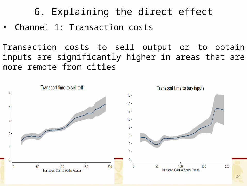
6. Explaining the direct effect• Channel 1: Transaction costs

Transaction costs to sell output or to obtain inputs are significantly higher in areas that are more remote from cities

25

6. Explaining the direct effect• Channel 2: Monetization of production factors

Significant drop in factor monetization, the more remote; more improved allocation of resources when better use of price signals?

26

6. Explaining the direct effect• Channel 3: Access to information and knowledge Significant association of urban proximity with access to extension agents, ownership of mobile phones, and awareness of improved technologies with urban proximity

27

7. Sensitivity analysis • Run four different regression set-ups (using the less parsimonious

SUR model):1. Add unobserved farming ability

2. Include opportunity costs of farmers’ time in transportation costs

3. Add squared transportation costs

4. Add a dummy that measures if teff was sold to Addis or not (and therefore test if direct link has a stronger effect on outcome variables)

• Results are robust to these four additional specifications

28

8. Conclusions • Link of urban areas with rural hinterland is not well understood,

especially so for staple crops, from which most farmers in Africa make a living.

• Study that issue in the case of Ethiopia, where in recent decades a significantly larger share of the rural population has become “connected” to a city (because of infrastructure development and city growth).

• Strong positive effect of urban proximity on:- Output prices but also on wages and land rental rates - Input and factor market use - Labor and land productivity - Profitability

29

8. Conclusions

• Changing price ratios of factor and output prices because of urban proximity important factor in explaining this effect (called “indirect effect”)

• However, other effects matter significantly as well (transaction costs, knowledge, information) (called “direct effect”)

• Beneficial effect of urbanization on intensification by rural producers of staple crops

• In contrast to rural population increases (population density increases) that do not show these positive effects on profitability and labor and land productivity

30

8. Conclusions

• Implications:

1. Access to markets and cities matter for rural populations and ensuring appropriate infrastructure and low transportation costs to access these markets for these rural populations is important

2. Cities an engine for agricultural transformation; ensuring that cities can grow such that rural areas can profit from these urban growth poles is important, e.g. stimulating rural-urban migration and improved tenure conditions.

3. Make sure that appropriate inputs and knowledge are there for the agricultural population so that they can profit from these new opportunities