Cities in Bad Shape: Urban Geometry in India�

Maria�avia Harariy

MIT

This version: 15 October 2014.Preliminary and incomplete. Please do not cite or circulate.

Abstract

The spatial layout of cities is an important determinant of urban commuting e¢ ciency.

This paper investigates the economic implications of urban geometry in the context of

India. A satellite-derived dataset of night-time lights is combined with historic maps to

retrieve the geometric properties of urban footprints in India over time. My approach

relies on a novel city-year level instrument for urban shape, which combines geography

with a mechanical model for city expansion. I investigate how city shape a¤ects the

location choices of consumers, in a spatial equilibrium framework à la Roback-Rosen.

Cities with more compact shapes are characterized by larger population, lower wages, and

higher housing rents, consistent with compact shape being a consumption amenity. The

implied welfare cost of deteriorating city shape is estimated to be sizeable. I also attempt

to shed light on policy responses to deteriorating shape. The adverse e¤ects of unfavorable

topography appear to be exacerbated by building height restrictions, and mitigated by

road infrastructure.

�I am grateful to my advisers Esther Du�o, Ben Olken and Dave Donaldson for their invaluable help

throughout this project. I also thank Alex Bartik, Jie Bai, Nathaniel Baum-Snow, Alain Bertaud, Melissa

Dell, John Firth, Ludovica Gazzè, Michael Greenstone, Gabriel Kreindler, Matthew Lowe, Rachael Meager,

Yuhei Miyauchi, Hoai-Luu Nguyen, Paul Novosad, Arianna Ornaghi, Bimal Patel, Champaka Rajagopal, Otis

Ried, Adam Sacarny, Albert Saiz, Ashish Shenoy, Chris Small, Kala Sridhar, William Wheaton and participants

to the MIT Development Lunch, Applied Micro Lunch and Development Seminar for helpful comments and

discussions at various stages of this work.yharari@mit.edu

1

1 Introduction

Most urban economics assumes implicitly that cities are circular or star-shaped. Real-world

cities, however, often depart signi�cantly from this assumption: cities display considerable

variation in shape. Urban geometries are jointly determined by a combination of geography and

policy (Bertaud, 2004). On the one hand, existing natural and topographic constraints prevent

cities from expanding radially in all directions. On the other, regulation and infrastructural

investment can a¤ect urban expansion both directly and indirectly. For instance, master plans

can explicitly promote polycentricity, by planning satellite centers around existing ones. Land

use regulations can encourage land consolidation, resulting in a more compact, as opposed

to fragmented development pattern. Investments in road infrastructure can encourage urban

growth along transport corridors.

While the economics literature has devoted very little attention to the geometry of cities,

in �elds such as urban planning and transportation engineering city shape is considered an

important determinant of commuting e¢ ciency, more compact shapes being characterized by

shorter trips and more cost-e¤ective transport networks. This, in turn, is claimed to a¤ect

productivity and welfare. Emphasizing the role of city shape in the functioning of public and

private transport, Bertaud (2004) argues that contiguous and compact urban development can

improve the welfare of city dwellers, by providing better and cheaper access to most of the

jobs. This is thought to be particularly relevant in the megacities of the developing world,

where most inhabitants cannot a¤ord individual means of transportation or where the large

size of the city precludes walking as a mean of getting to jobs. Cervero (2002) emphasizes

how compact, accessible cities are potentially more productive, through a combination of labor

market pooling, savings in transporting inputs and technological and information spillovers.

This urban planning literature is mostly descriptive

In this paper I investigate empirically the economic implications of city shape in the context

of India. More speci�cally, I examine two complementary sets of questions: �rst, how city

geometry a¤ects the location choices of consumers, in the framework of spatial equilibrium

across cities, and what the welfare implications of deteriorating city shape are. Second, how

policy interacts with geography in determining urban form.

India represents a promising setting to study urban spatial structures for a number of reasons.

First, as most developing countries, India is experiencing fast urban growth. According to the

2

2011 Census, the urban population amounts to 377 million, increasing from 285 million in 2001

and 217 million in 1991, representing between 25 and 31 percent of the total. Although the pace

of urbanization is slower than in other Asian countries, it is accelerating, and it is predicted

that another 250 million will join the urban ranks by 2030 (Mc Kinsey, 2010). This growth

in population has been accompanied by a signi�cant physical expansion of urban footprints,

typically beyond urban administrative boundaries (Indian Institute of Human Settlements,

2013; World Bank, 2013). This setting thus provides a unique opportunity to observe the

shapes of cities as they evolve and expand over time. Such an exercise would not be feasible

in a developed context: urban spatial structures in developed countries are typically very

resilient and path dependent (Bertaud, 2004), which would prevent me from detecting signi�cant

variation over time.

Secondly, India is characterized by a di¤used urbanization pattern. With an unusually large

number of highly-populated cities, India contrasts from other developing countries characterized

by the presence of a large capital city and very few other urban centers. This ensures a large

enough sample of cities for the econometric analyses which I carry out.

Moreover, the challenges posed by urban expansion have been gaining increasing importance

in India�s policy discourse, which makes it particularly relevant to investigate these matters from

an economics perspective. On the one hand, this debate has focused on the perceived harms of

haphazardous urban expansion, most notably limited urban mobility and lengthy commutes.

According to a recent Mc Kinsey report (2010), the average peak morning commute in Indian

million-plus cities is in excess of one-and-a-half to two hours. Providing e¤ective urban public

transit systems has been consistently identi�ed as a key policy recommendation for the near

future (e.g. Mitric and Chatterton, 2005; World Bank, 2013; Mc Kinsey, 2013.). On the other

hand, there is a growing concern that existing policies �in particular, urban land use regulations

�might directly or indirectly contribute to distorting urban form (World Bank, 2013, Sridhar,

2010, Glaeser, 2011). The most paradigmatic of these measures are restrictions on building

height, in the form of Floor Area Ratios (FARs). FARs in Indian cities are considered very

restrictive compared to international standards, and have been indicated as one of the causes of

sprawl in Indian cities (Brueckner and Sridhar, 2012; Bertaud and Brueckner, 2005). Another

example is given by the Urban Land Ceiling and Regulation Act, which has been claimed to

hinder intra-urban land consolidation and restrict the supply of land available for development

within cities (Sridhar, 2010).

3

My broad research question concerns the economic implications of city shape. In particular,

in this project I am interested in two complementary sets of issues. The �rst and main question

relates to how city shape a¤ects the location choices of consumers across cities. I investigate this

in the framework of a model of spatial equilibrium across cities à la Roback-Rosen, modelling

city shape as an amenity. My �ndings are broadly consistent with "good city shape" being a

consumption amenity. I �nd robust evidence that cities with more compact shapes grow faster,

all else being equal. There is also some evidence that consumers are paying a premium in terms

of lower wages and higher rents in order to live in cities with better geometries. I estimate the

implied welfare cost of deteriorating shape, �nding that it is sizeable and considerably larger

than the mere monetary cost associated to lengthier commutes.

A natural question which arises next concerns the role of policy: if city shape indeed has

welfare implications, what is the optimal policy response to existing topographic constraints?

Although a thorough investigation of this question might require more detailed data than those

used in this study, in the concluding part of this paper I make a preliminary attempt to explore

the interactions between topography, regulation and city shape. I �nd that restrictions on

building height - in the form of low FARs - result in cities which are more spread out in space

and less compact than their topography would predict. This is consistent with one of the

most common arguments against restrictive FARs in India, namely that they cause sprawl by

preventing cities from growing vertically (Glaeser, 2011).

My methodology can be outlined as follows. The bulk of my empirical analysis is conducted

at the city-year level and is based on an instrumental variable approach. I assemble an un-

balanced panel dataset of urban footprints for about 400 Indian cities, by combining historic

maps (1950) with a satellite-derived dataset of night-time lights (1992-2010). I compute sev-

eral geometric indicators for urban shape, used in urban planning as proxies for the patterns

of within-city trips. I develop an original instrument for city shape by combining geography

with a mechanical model for city expansion. The underlying idea is that, as cities expand in

space, they face di¤erent geographic constraints - steep terrain or water bodies - leading to

departures from an ideal circular expansion path. The construction of my instrument requires

two steps. First, I use a mechanical model for city expansion to predict the area which a city

should occupy in a given year. I consider two versions of this model: one based on each city�s

historic population growth rates, and one postulating a common growth rate for all cities. Sec-

4

ond, I consider the largest contiguous patch of developable land within this predicted radius

("potential footprint") and compute its shape properties. I then proceed to instrument the

shape properties of the actual city footprint in that given year with the shape properties of

the potential footprint. The resulting instrument varies at the city-year level, allowing me to

control for time-invariant city characteristics through city �xed e¤ects. The identi�cation of

the impact of shape thus relies on comparing geography-driven changes in urban shape over

time for each city. My main results are summarized below.

(i) I �nd a strong, robust �rst stage linking the actual shape that a city�s footprint has at a

given point in time and the potential shape which it can have given the layout of the geographic

constraints surrounding it. This is not solely driven by extremely constrained topographies (e.g.

coastal or mountainous cities) in my sample.

(ii) There is a strong and robust negative IV relationship between population and non-

compactness, conditional on area. My most conservative estimate indicates that a one standard-

deviation deterioration in city shape entails decrease in population density of 0.9 standard

deviations.

(iii) There is suggestive evidence that households are paying for compact geometry both

through higher housing prices and through lower wages. Using district level averages as proxies

for city-level data, I �nd a marginally signi�cant negative relationship between non-compactness

and rents per square meter, and a positive relationship between non-compactness and wages.

Although noisy, these results are consistent with "good shape" being valued a consumption

amenity. Using these estimates in conjunction with a simple version of the Rosen-Roback

model, I �nd that a one standard deviation deterioration in city shape entails a welfare loss

equivalent to a 5% decrease in income.

(iv) Interacting city shape with di¤erent proxies for infrastructure, I �nd that the negative

e¤ects of poor geometry on population growth are mitigated by a denser road network and by

the availability of motor vehicles, suggesting that commute times could be the main mechanism

through which city shape a¤ects consumers.

(v) Cities with poorer shapes are characterized by comparatively fewer slum dwellers and

houses of better quality. This is consistent with the interpretation that low-income immigrants

tend to sort into more compact cities, possibly because they are less able to cope with lengthy

commutes.

The �nal part of my work attempts to look at the endogenous responses to unfavorable city

5

shape. Due to data limitations, most of these results are based on a cross-section of cities only,

and should therefore be interpreted as suggestive.

(vi) Restrictive FARs result in footprints which are both larger and less compact. Higher

FARs, on the other hand, mitigate the negative e¤ects of poor geometry on population growth.

(vii) Cities with worse geometries appear to have a less dense road network in absolute terms,

but road density per capita is not signi�cantly di¤erent from that observed in more compact

cities.

(viii) Productive establishments appear less spatially concentrated in non-compact cities.

This could re�ect a tendency of cities to become less monocentric as their shape deteriorates.

This projects contributes to the existing literature in a number of directions. The �rst

concerns the analysis of urban geometry from an economics standpoint. To my knowledge,

this is the �rst work which studies city shape as an amenity. The second is methodological

and relates to the measurement of the properties of urban footprints. I employ the OLS night-

time lights dataset to track the shape of urban footprints over time, following an approach

which has been used in urban remote sensing, but not in economics. The use of shape metrics

borrowed from the urban planning literature to measure economically relevant properties of

urban footprints is also novel. Furthermore, I develop an original instrument for city shape,

which is potentially applicable to other contexts as well.

The remainder of the paper is organized as follows. Section 2 brie�y reviews the existing

literature. Section 3 outlines the conceptual framework. Section 4 documents my data sources

and describes the geometric indicators which I employ. Section 5 presents my empirical strategy

and describes in detail how my instrument is constructed. The empirical evidence is presented

in the following two Sections. Section 6 discusses my main results, which pertain to the e¤ects

of city shape on the location choices of consumers. Section 7 provides some results on other

endogenous responses to city shape, including interactions between topography and policy.

Section 8 concludes with indications for future work.

2 Previous Literature

The economics literature on urban spatial structures has mostly focused on two aspects of urban

form: city size and population density gradient. The classic monocentric city model (Alonso,

6

1964; Mills, 1967, 1972; Muth, 1969) postulates the existence of a single employment center

and predicts the formation of a circular city with declining density gradient, and whose radius

declines with transportation costs. Richer polycentric city models were subsequent developed,

where the number, location and spatial extent of employment centers are determined endoge-

nously in a linear or circular city (Fujita and Ogawa, 1982, Lucas and Rossi-Hansberg, 2002).

Although these models can in principle be altered to generate non-circular cities, for instance,

assuming the road network is not radial (Brueckner, 2011, p. 56), the focus of this literature

is on the determinants of the internal structure of cities, and the implications of geometry are

left unexplored. My approach is di¤erent since I take the shape of each city as given and I

investigate its e¤ects on the spatial equilibrium across, rather than within cities.

The conceptual framework I draw upon is that on spatial equilibrium across cities, after

Rosen(1979) and Roback(1982). In the simplest version of this model, consumers and �rms

endogenously choose to locate in cities with di¤erent levels of amenities, and wages and rents

adjust to equalize utility across locations. I model "compact city shape" as an amenity, which

a¤ects consumers and �rms primarily by reducing the length of within-city trips. Although

Glaeser (2008) acknowledges that amenities presumably include also commuting times, I am

not aware of studies explicitly looking at the link between commuting, urban geometry and the

spatial equilibrium across cities. A large empirical literature has employed the classic Rosen-

Roback framework to investigate the value of amenities (e.g. Blomquist, 1988). This literature,

however, has almost exclusively focused on the US, and has not always adequately addressed

the endogeneity of amenities (Gyourko, Kahn and Tracy, 1999).

A large empirical literature investigates urban sprawl (Glaeser and Kahn, 2004; Burch�eld

et al, 2006), typically in the context of the US. Although there is not a single de�nition of

sprawl, some studies identify sprawl with non-contiguous development (Burch�eld et al, 2006),

which is somewhat related to the notion of "compactness" which I investigate. In most analyses

of sprawl, however, the focus is on decentralization and density. I focus on a di¤erent set of

spatial properties of urban footprints: conditional on the overall amount of land used, I look

at geometric properties aimed at proxying the pattern of within-city trips. My work is more

closely related to that of Bento et al (2005), who incorporate a measure of city shape in their

investigation of the link between urban form and travel demand. However, their analysis is

based on a cross-section of US cities and does not address the endogeneity of city shape.

7

The geometric indicators of city shape which I employ are borrowed from the urban planning

and landscape ecology literature (Angel and Civco, 2009; Angel et al., 2009), which is mostly

descriptive. Urban planners emphasize the link between city shape, average intra-urban trip

length and accessibility, claiming that contiguous, compact and predominantly monocentric

urban morphologies are more favorable to transit. Bertaud (2004) argues that more compact

cities are generally more favorable to the poor, since they provide better access to jobs, but at

the same time have higher land prices, which would tend to reduce their housing �oor space

consumption. Cervero (2002) emphasizes how compact, accessible cities are potentially more

productive, through a combination of labor market pooling, savings in transporting inputs and

technological and information spillovers, and shows a correlation between labor productivity

and accessibility in US cities1.

In terms of methodology, my work is related to that of Burch�eld et al. (2006), who also

employ remotely sensed data to track urban areas over time. More speci�cally, they analyze

changes in the extent of sprawl in US cities between 1992 and 1996. The data I employ comes

mostly from night-time, as opposed to day-time imagery, and covers a longer time span (1992-

2010).

Saiz (2011) also looks at geographic constraints to city expansion, by computing the amount

of developable land within 50 km radii from US city centers and relating it to the elasticity of

housing supply. I use the same notion of geographic constraints, but I employ them in a novel

way to construct a time-varying instrument for city shape.

Finally, my work is also related to a growing literature on road infrastructure and urban

growth in developing countries (Baum-Snow and Turner, 2012; Baum-Snow et al., 2013; Morten

and Oliveira, 2014, Storeygard, 2014). In particular, Morten and Oliveira (2014) also estimate

a model of spatial equilibrium across cities, and resort to an instrumental variables approach.

Di¤erently from these studies, I do not look at the impact of roads connecting cities, but instead

focus on urban geometry as a proxy for the trips within cities.

1A subset of the urban planning and evironmental literature (reviewed by Martins et al, 2012) also looks

at the environmental implications of city shape. Bertaud (2002, 2004) argues that although compact cities are

characterized by shorter trip patterns, they might not necessarily be less polluted due to potential higher density

of motor vehicles. Most empirical analyses (e.g. Clark et al. 2011) �nd that more compact and denser cities

are less polluted, but do not separately identify the e¤ect of shape and that of density.

8

3 Conceptual Framework

In this study I interpret city shape to �rst-order as a shifter of commuting costs: all else being

equal, including city size, a city with a more compact geometry is characterized by shorter

within-city trips2. It is plausible that consumers incorporate considerations on the relative

ease of commutes when evaluating the trade-o¤s associated to di¤erent locations. This might

be even more relevant in the context of India, in which most migrants to urban areas cannot

a¤ord individual means of transport. A natural starting point in thinking how city shape

a¤ects the location choices of consumers is to interpret "good geometry" as an amenity, in the

framework of a model of spatial equilibrium à la the Rosen-Roback (Rosen 1979, Roback, 1982).

The basic underlying idea of the Rosen-Roback model is that consumers and �rms must be

indi¤erent across cities, and wages and rents allocate people and �rms to cities with di¤erent

levels of amenities. The notion of spatial equilibrium across cities presumes that consumers

are choosing across a number of di¤erent locations. The pattern of migration to urban areas

observed in India is compatible with this element of choice: according to the 2001 Census, about

38 percent of internal migrants move to a location outside their district of origin, supporting

the interpretation that they are e¤ectively choosing a city rather than simply moving to the

closest available urban location.

I draw upon the Roback model in its simplest form (Roback, 1982), following the exposition

of the model by Glaeser (2008). Households consume a composite good C and housing H. They

supply inelastically one unit of labor receiving a city-speci�c wage W . Their utility depends on

net income, i.e. labor income minus housing costs, and on a city-speci�c bundle of consumption

amenities �. Their optimization problem reads:

maxC;H

U(C;H; �) s:t: C = W � phH (1)

where ph is the rental price of housing and

U(C;H; �) = �C1��H�: (2)

In equilibrium, indirect utility V must be equalized across cities, otherwise workers would move:

V (W � phH; �) = � (3)

2In Section 4.2 I illustrate the geometric indicators I employ to measure compactness, which are all based on

the relative distances between points within a footprint. In Section 8 I discuss brie�y other possible second-order

channels through whih city shape might a¤ect consumers.

9

which given the functional form assumptions yields the condition

log(W )� � log(ph) + log(�) = V : (4)

The intuition for this condition is that consumers pay for amenities through lower wages (W )

or through higher housing prices (ph). The extent to which wages net of housing costs rise

with an amenity is a measure of the extent to which that amenity decreases utility, relative to

the marginal utility of income. Di¤erentiating this expression with respect to some exogenous

variable S - which could be (instrumented) city geometry - yields:

@ log(�)

@S= �

@ log(ph)

@S� @ log(W )

@S: (5)

This equation provides a way to evaluate the amenity value of S: the overall impact of S on

utility can be found as the di¤erence between the impact of S on housing prices, multiplied by

the share of housing in consumption, and the impact of S on wages.

Firms in the production sector also choose optimally in which city to locate. Each city is a

competitive economy that produces a single internationally traded good Y using labor N and a

local production amenity A. Their technology also requires traded capital K and a �xed supply

of non-traded capital Z. Firms solve the following production maximization problem:

maxN;K

�Y (N;K;Z;A)�WN �K

(6)

where

Y (N;K;Z;A) = AN�K Z1���

: (7)

In equilibrium �rms earn zero expected pro�ts, which are equalized across cities. Under these

functional form assumptions, the maximization problem for �rms yields the following labor

demand condition:

(1� ) log(W ) = (1� � � )(log(Z)� log(N)) + log(A) + �1: (8)

To close the model we need to specify the construction sector. Developers produce housing H

using land l and "building height" h. In each location there is a �xed supply of land L, as a

result of land use regulations3. Denoting with pl the price of land, their maximization problem

3In this framework, the amount of land to be developed is assumed to be given in the short run. It can be

argued that in reality it is an endogenous outcome of factors such as quality of regulation, success of the city

and geographic constraints. In my empirical analysis, city area will be speci�ed as a mechanical function of

predicted population growth, thus abstracting from these issues (see Section 5.2, Speci�cation I).

10

reads:

maxHfphH � C(H)g (9)

where

H = l � h (10)

C(H) = c0h�l � pll , � > 1: (11)

The construction sector operates optimally, with construction pro�ts equalized across cities.

By combining the housing supply equation resulting from the maximization problem of devel-

opers with the housing demand equation resulting from the consumers�problem, we obtain the

following housing market equilibrium condition:

(� � 1) log(H) = log(ph)� log(c0�)� (� � 1) log(N) + (� � 1) log(L) (12)

Using the three optimality conditions for consumers (4), �rms (8) and (12) this model can be

solved for the three unknowns N , W and ph , representing respectively population, wages and

housing prices, as functions of the model parameters and in particular as functions of the city

speci�c productivity parameter and consumption amenities. Denoting all constants with K,

this yields the following:

log(N) =(�(1� �) + �) log(A) + (1� )

�� log(�) + �(� � 1) log(L)

��(1� � � ) + ��(� � 1) +KN (13)

log(W ) =(� � 1)� log(A)� (1� � � )

�� log(�) + �(� � 1) log(L)

��(1� � � ) + ��(� � 1) +KW (14)

log(ph) =(� � 1)

�log(A) + � log(�)� (1� � � ) log(L)

��(1� � � ) + ��(� � 1) +KP : (15)

These conditions translate into the following predictions:

d log(N)

d log(A)> 0;

d log(N)

d log(�)> 0;

d log(N)

d log(L)> 0 (16)

d log(W )

d log(A)> 0;

d log(W )

d log(�)< 0;

d log(W )

d log(L)< 0 (17)

d log(ph)

d log(A)> 0;

d log(ph)

d log(�)> 0;

d log(ph)

d log(L)< 0: (18)

Population, wages and rents are all increasing functions of the city-speci�c productivity para-

meter. Population and rents are increasing in the amenity parameter as well, whereas wages

11

are decreasing in it. The intuition is that �rms and consumers have potentially con�icting

location preferences: �rms prefer cities with higher production amenities, whereas consumers

prefer cities with higher consumption amenities. Factor prices �W and pH �are striking the

balance between these con�icting preferences.

Consider now an indicator of urban geometry S, higher values of S denoting "worse" shapes,

in the sense of shapes conducive to longer commute trips. Assume "non-compact shape" is

purely a consumption disamenity, which decreases consumers�utility all else being equal but

does not directly a¤ect �rms�productivity:

@�

@S< 0;

@A

@S= 0 (19)

In this case we should observe the following reduced-form relationships:

dN

dS< 0;

dW

dS> 0;

dphdS

< 0 (20)

This framework predicts that a city with poorer shape should have ceteris paribus a smaller

population, higher wages and lower house rents. The intuition is that consumers prefer to

live in cities with good shapes, which drives rents up and bids wages down in these locations.

Suppose instead that poor city geometry is both a consumption and a production disamenity,

i.e. it depresses both the utility of consumers and the productivity of �rms:

@�

@S< 0;

@A

@S< 0 (21)

This would imply the following:

dN

dS< 0;

dW

dS? 0; dph

dS< 0 (22)

The model�s predictions are similar, except that the e¤ect on wages will be ambiguous. The

reason for the ambiguous sign of dWdSis that now both �rms and consumers want to locate in

compact cities. With respect to the previous case, we now have an additional force which tends

to bid wages up in compact cities: competition among �rms for locating in low-S cities. The

net e¤ect on W depends on on whether �rms or consumers value low S the most. If S is more

a consumption than it is a production disamenity, then we should observe dWdS> 0:

Assume now that

log(A) = �A + �AS (23)

log(�) = �� + ��S: (24)

12

Plugging (23) and (24) into (13),(14) and (15) we obtain:

log(N) =[(�(1� �) + �)�A + (1� )���] � S + (1� )�(� � 1) log(L)

�(1� � � ) + ��(� � 1) +KN (25)

log(W ) =[(� � 1)��A � (1� � � )���] � S � (1� � � )�(� � 1) log(L)

�(1� � � ) + ��(� � 1) +KW (26)

log(ph) =[(� � 1)�A + (� � 1)���] � S � (1� � � )(� � 1) log(L)

�(1� � � ) + ��(� � 1) +KP : (27)

For ease of exposition, de�ne:

BN =(�(1� �) + �)�A + (1� )����(1� � � ) + ��(� � 1) ; LN =

(1� )�(� � 1)�(1� � � ) + ��(� � 1) (28)

BW =(� � 1)��A � (1� � � )����(1� � � ) + ��(� � 1) ; LW =

�(1� � � )�(� � 1)�(1� � � ) + ��(� � 1) (29)

BP =(� � 1)�A + (� � 1)����(1� � � ) + ��(� � 1) ; LP =

�(1� � � )(� � 1)�(1� � � ) + ��(� � 1) : (30)

This allows us to rewrite (25); (26); (27) in a more parsimonious form:

log(N) = BNS + LN log(L) +KN (31)

log(W ) = BWS + LW log(L) +KW (32)

log(ph) = BPS + LP log(L) +KP : (33)

Note that (28); (29); (30) imply:

�A = (1� � � )BN + (1� )BW (34)

�� = �BP �BW : (35)

The welfare impact of a marginal increase in S can be quanti�ed using equation (5), which

states that in equilibrium a marginal change in log(�) needs to be compensated 1 to 1 by a

change in log(W ) :

@ log(�)

@S= �� = �

@ log(ph)

@S� @ log(W )

@S= �BP �BW : (36)

Parameter �� captures, in log points, the welfare loss form a marginal increase in S. Parameter

�A captures the impact of a marginal increase in S on city-speci�c productivity. Denote withcBN ;dBW and cBP the reduced-form estimates for the impact of S on respectively log(N); log(W )13

and log(ph):These estimates, in conjunction with plausible values for parameters �; ; �, can be

used to back out �A and ��:

c�A = (1� � � )cBN + (1� )dBW (37)b�� = �cBP �dBW : (38)

Note that this approach captures the overall, net e¤ect of S on the average city dweller, with-

out explicitly modelling the mechanism through which S enters the decisions of consumers. In

Section 6.2 I provide empirical evidence suggesting that the urban transit channel is indeed in-

volved, and in the concluding section I discuss some alternative, second-order channels through

which city shape might a¤ect consumers. This simple model also does not explicitly address

heterogeneity across consumers in tastes and skills. However, we expect that people will sort

themselves into locations based on their preferences. The estimated di¤erences in wages and

rents across cities will thus be an underestimate of true equalizing di¤erences for those with a

strong taste for the amenity of interest, and an overestimate for those with weak preferences.

The empirical evidence presented in Section 6.2 indicates that there might indeed be sorting

across cities with di¤erent geometries.

Reduced-form estimates for BN ; BW ; BP are presented in Sections 6.1 and 6.2, whereas Sec-

tion 6.3 provides estimates for the structural parameters �A; ��:The next two Sections present

the data sources and empirical strategy employed in the estimation.

4 Data Sources

I assemble an unbalanced panel of urban footprints-years, covering all Indian cities for which a

footprint could be retrieved based on the methodology explained below.

4.1 Urban Footprints

I retrieve the boundaries of urban footprints from two sources. The �rst is the U.S. Army India

and Pakistan Topographic Maps (U.S. Army Map Service, 195?), a series of detailed maps

covering the entire Indian subcontinent at a 1:250,000 scale. I geo-referenced these maps and

traced the reported perimeter of urban areas, which are clearly demarcated (Figure 1).

The second source is derived from the DMSP/OLS Night-time Lights dataset. This dataset

14

is based on night-time imagery recorded by satellites from the U.S. Air Force Defense Meteo-

rological Satellite Program (DMSP) and reports the recorded intensity of Earth-based lights,

measured by a six-bit number (ranging from 0 to 63). These data are reported for every year

between 1992 and 2010, with a resolution of 30 arc-seconds (approximately 1 square kilome-

ters). Night-time lights have been employed in economics typically for purposes other than

urban mapping (Henderson et al., 2012). However, the use of the DMSP/OLS dataset for de-

lineating urban areas is quite common in urban remote sensing (Henderson et al., 2003; Small,

2005; Small et al. 2011). The basic methodology is the following: �rst, I overlap the night-time

lights imagery with a point shape�le with the coordinates of Indian settlement points, taken

from the Global Rural-Urban Mapping Project (GRUMP) Settlement Points dataset (CIESIN

et al., 2011; Balk et al., 2006). I then set a luminosity threshold (e.g. 35) and consider spatially

contiguous lighted areas surrounding the city coordinates with luminosity above that thresh-

old. This approach, illustrated in Figure 2, can be replicated for every year covered by the

DMSP/OLS dataset.

The choice of luminosity threshold results in a more or less restrictive de�nition of urban

areas, which will appear larger for lower thresholds4. To choose luminosity thresholds appropri-

ate for India, I overlap the 2010 night-time lights imagery with available Google Earth imagery.

I �nd that a luminosity threshold of 35 generates the most plausible mapping for those cities

covered by both sources5. In my full panel (including years 1950 and 1992-2010), the average

city footprint occupies and area of approximately 63 squared kilometers6.

Using night-time lights as opposed to alternative satellite-based products, in particular day-

time imagery, is motivated by a number of advantages. Unlike products such as aerial pho-

tographs or high-resolution imagery, night-time lights cover systematically the entire Indian

4Determining where to place the boundary between urban and rural areas always entails some degree of

arbitrariness, and in the urban remote sensing literature there is no clear consensus on how to set such threshold.

It is nevertheless recommended to validate the chosen threshold by comparing the DMSP/OLS-based urban

mapping with alternative sources, such as high-resolution day-time imagery, which in the case of India is

available only for a small subset of city-years.5For years covered by both sources (1990, 1995, 2000), my maps also appear consistent with those from the

GRUMP - Urban Extents Grid dataset, which combines night-time lights with administrative and Census data

to produce global urban maps (CIESIN et al., 2011; Balk et al., 2006).6My results are robust to using alternative luminosity thresholds between 20 and 40. Results are available

upon request.

15

subcontinent, and not only a selected number of cities. Moreover, they are one of the few

sources which allow to detect changes in urban areas over time, due to their yearly temporal

frequency. Finally, unlike multi-spectral satellite imagery such as Landsat- or MODIS- based

products, which in principle would be available for di¤erent points in time, night-time lights

do not require any sophisticated manual pre-processing7. An extensive portion of the urban

remote sensing literature compares the accuracy of this approach in mapping urban areas with

that attainable with alternative satellite-based products, in particular day-time imagery (in-

ter alia, Henderson et al, 2003; Small et al., 2005). This cross-validation exercise has been

carried out also speci�cally in the context of India by Joshi et al. (2011) and Roychowdhury

(2009). The general takeout is that none of these sources is error-free, and that there is no

strong case for preferring day-time over night-time satellite imagery if aerial photographs are

not systematically available for the area to be mapped.

It is well known that urban maps based on night-time lights will tend to in�ate urban

boundaries, due to "blooming" e¤ects (Small et al., 2005)8. This can only partially be limited

by setting high luminosity thresholds. In my panel, urban footprints as reported for years

1992-2010 thus re�ect a broad de�nition of urban agglomeration, which typically goes beyond

the current administrative boundaries. This contrasts with urban boundaries reported in the

US Army maps, which seem to re�ect a more restrictive de�nition of urban areas (although

no speci�c documentation is available). Throughout my analysis I include year �xed e¤ects,

which amongst other things control for these di¤erences in data sources, as well as for di¤erent

calibrations of the night-time lights satellites.

By combining the US Army maps (1950s) with yearly maps obtained from the night-time

lights dataset (1992-2010) I thus assemble an unbalanced panel of urban footprints9. The criteria

7Using multi-spectral imagery to map urban areas requires a manual classi�cation process, which relies

extensively on alternative sources, mostly aerial photographs, to cross-validate the spectral recognition, and is

subject to human bias.8DMSP-OLS night-time imagery has a tendency to overestimate the actual extent of lit area on the ground,

due to a combination of coarse spatial resolution, overlap between pixels, and minor geolocation errors (Small

et al., 2005).9The resulting panel dataset is unbalanced for two reasons: �rst, some settlements become large enough to

be detectable only later in the panel; second, some settlements appear as individual cities for some years in

the panel and then become part of larger urban agglomerations in later years.The number of cities in the panel

ranges from 352 to 457, depending on the year considered.

16

for being included in the analysis is to appear as a contiguous lighted shape in the night-time

lights dataset. This appears to leave out only very small settlements. Throughout my analysis,

I instrument all the geometric properties of urban footprints, including both area and shape.

This IV approach addresses problems of non-classical measurement error which could a¤ect my

data sources, for instance due to the well-known correlation between income and luminosity.

4.2 Shape Metrics

The indicators of city shape which I employ, based on those in Angel, Civco and Parent (2010)10,

are used in landscape ecology and urban studies to proxy for within-city trips and infer travel

costs. They are all based on the distribution of points around the polygon�s centroid11 or within

the polygon, and are measured in kilometers. Summary statistics for the indicators below are

reported in Table 1.

(i) The remoteness index is the average distance between all interior points and the centroid.

It can be considered a proxy for the average length of commutes to the urban center.

(ii) The spin index is computed as the average of the squared distances between interior

points and centroid. This is similar to the remoteness index, but gives more weight to the

polygon�s extremities, corresponding to the periphery of the footprint. This index is more

capable of identifying footprints that have "tendril-like" projections, often perceived as an

indicator of sprawl.

(iii) The disconnection index captures the average distance between all pairs of interior

points. It can be considered a proxy for commutes within the city, without restricting one�s

attention to those leading to the center.

(iv) The range index captures the maximum distance between two points on the shape

perimeter, representing the longest possible of commute trips within the city.

All these measures are mechanically correlated with polygon area. In order to separate the

e¤ect of geometry per se from that of city size, in my preferred speci�cations I explicitly control

for the area of the footprint - which is separately instrumented for. Conditional footprint area,

10I am thankful to Vit Paszto for help with the ArcGis shape metrics routines. I have renamed some of the

shape metrics for ease of exposition.11The centroid of a polygon, or center of gravity, is the point which minimizes the sum of squared Euclidean

distances between itself and each vertex.

17

higher values of these indexes indicate longer within-city trips. Alternatively,it is possible to

normalize each of these indexes, computing a version which is invariant to the area of the

polygon. I do so by computing �rst the radius of the "Equivalent Area Circle" (EAC), namely

a circle with an area equal to that of the polygon. I then normalize the index of interest dividing

it by the EAC radius, obtaining what I de�ne normalized remoteness, normalized spin, etc. One

way to interpret these normalized metrics is as deviations of a polygon�s shape from that of a

circle, the shape which minimizes all the indexes above.

Figure 3 provides a visual example of how these metrics map to the shape of urban foot-

prints. Among million-plus cities, I consider those with respectively the "best" and the "worst"

geometry based on the indicators described above, namely Bengaluru and Kolkata (formerly

known as Bangalore and Calcutta). The �gure reports the footprints of the two cities as of year

2005, where Bengaluru�s footprint has been rescaled so that they have the same area. The

�gure also reports the above shape metrics computed for these two footprints. The di¤erence

in the remoteness index between Kolkata and (rescaled) Bengaluru is 4.5 km; the di¤erence

in the disconnection index is 6.2 km. The interpretation is the following: if Kolkata had the

same compact shape that Bengaluru has, the average trip to the center would be shorter by

4.5 km and the average trip within the city would be shorter by 6.2 km. The Indian Ministry

of Urban Development (2008) estimates the average commute speed in million-plus cities to be

of 12 km per hour in 2011, which is predicted to become 9 km by 2021. According to the 2011

estimated speed, the above di¤erences in trip length translate to a di¤erence in commute times

of respectively 22.5 minutes (average trip to the center) and 31 minutes (average within-city

trip). Although this is a very rough calculation, it is nevertheless revealing that city geometry

indeed has potentially sizeable impacts on commute times.

4.3 Geography

Following Saiz (2011), I consider as "undevelopable" terrain which either covered by a water

body or is characterized by a slope above 15%. I draw upon the highest resolution sources

available: the Advanced Spaceborne Thermal Emission and Re�ection Radiometer (ASTER)

Global Digital Elevation Model (NASA and METI, 2011), with a resolution of 30 meters, and

the Global MODIS Raster Water Mask (Carroll et al. 2009), with a resolution of 250 meters. I

combine these two raster datasets to classify pixels as "developable" or "undevelopable". Figure

18

4 illustrates this classi�cation for the Mumbai area.

4.4 Population and Other Census Data

City-level data for India is notoriously hard to obtain (Greenstone and Hanna, forthcoming).

The only systematic source which collects data explicitly at the city level is the Census of

India, conducted every 10 years. In this project I employ population data from Census years

1871-2011. As explained in Section 5.1, historic population (1871-1941) is used to construct

one of the two versions of my instrument, whereas population drawn from more recent waves

(1951, 1991, 2001 and 2011) is used as an outcome variable12.

Outcomes other than population are not consistently available for all Census years. I draw

data on urban road length in 1991 from the 1991 Town Directory. In recent Census waves

(1991, 2001, 2011) data on slum population and physical characteristics of houses are available

for a subset of cities.

It is worth pointing out that "footprints" as retrieved from the night-time lights dataset do

not always have an immediate Census counterpart in terms of town or urban agglomeration, as

they sometimes stretch to include suburbs and towns treated as separate units by the Census.

A paradigmatic example is the Delhi conurbation, which as seen from the satellite expands

well beyond the administrative boundaries of the New Delhi National Capital Region. When

assigning population totals to an urban footprint, I sum the population of all Census settlements

which are located within the footprint, thus computing a "footprint" population total13.

4.5 Wages and Rents

For outcomes other than those available in the Census I rely on the National Sample Survey

and the Annual Survey of Industries, which provide at most district identi�ers. I thus follow the

approach of Greenstone and Hanna (forthcoming): I match cities to districts and use district

urban averages as proxies for city-level averages. It should be noted that the matching is not

12Historic population totals were taken from Mitra (1980). Census data for years 1991 to 2001

were taken from the Census of India electronic format releases. 2011 Census data were retrieved from

http://www.censusindia.gov.in/DigitalLibrary/Archive_home.aspx.13In order to assemble a consistent panel of city population totals over the years I also take into account

changes in the de�nitions of "urban agglomerations" and "outgrowths" across Census waves.

19

always perfect, for a number of reasons. First, it is not always possible to match districts as

reported in these sources to Census districts, and through these to cities, due to redistricting

and inconsistent numbering throughout this period. Second, there are a few cases of large

cities which cut across districts (e.g. Hyderabad). Finally, there are a number of districts

which contain more than one city from my sample. In these cases I follow several matching

approaches: considering only the main city for that district, and dropping the district entirely.

I show results following both approaches. The matching process introduces considerable noise

and leads to results which are relatively less precise and less robust than those I obtain with

city-level outcomes.

Data on wages are taken from the Annual Survey of Industries (ASI), waves 1990, 1994, 1995,

1997, 1998, 2009, 201014. These are repeated cross-sections of plant-level data collected by the

Ministry of Programme Planning and Implementation of the Government of India. The ASI

covers all registered manufacturing plants in India with more than �fty workers (one hundred

if without power) and a random one-third sample of registered plants with more than ten

workers (twenty if without power) but less than �fty (or one hundred) workers. As mentioned

by Fernandes and Sharma (2012) amongst others, the ASI data are extremely noisy in some

years, which introduces a further source of measurement error. The average individual yearly

wage in this panel amounts to 94 thousand Rs. at current prices.

Unfortunately there is no systematic source of data for property prices in India. I construct

a rough proxy for the rental price of housing drawing upon the National Sample Survey (House-

hold Consumer Expenditure schedule), which asks households about the amount spent on rent.

In the case of owned houses, an imputed �gure is provided. I focus on rounds 62 (2005-2006),

63 (2006-2007) and 64 (2007-2008), since they are the only ones for which the urban data is

representative at the district level and which report total dwelling �oor area as well. I use this

information to construct a measure of rent per square meter. The average yearly total rent paid

in this sample amounts to about 25 thousand Rs., whereas the average yearly rent per squared

meter is 603 Rs., at current prices. These �gures are likely to be underestimating the market

rental rate, due to the presence of rent control provisions in most major cities of India (Dek,

2006). To cope with this problem, I also construct an alternative proxy for housing rents which

focuses on the upper half of the distribution of rents per meter, which is less likely to include

14These are all the waves I could access as of June 2014.

20

observations from rent-controlled housing.

4.6 Other Data

Data on state-level infrastructure (motor vehicles density, state urban roads length) is taken

from the Ministry of Road Transport and Highways, Govt. of India.

Data on the current road network is constructed from the maps available on Openstreetmap15,

a collaborative mapping project which provides crowdsourced maps of the world. Open-

streetmap data has been favorably compared with proprietary data sources and is continuously

updated. As such, it re�ects the current state of the street network. I consider the most recent

night-time lights-based map of urban boundaries in my sample - corresponding to 2010 - and

overlap it with the street network map of India provided by Openstreetmap. Information on

the type of road - whether trunk, residential, secondary etc. - is also provided. Given the

collaborative nature of Openstreetmap, there is a concern that the level of detail of such maps

might be higher in larger cities, or in neighborhoods with more economic activity. Upon visual

inspection, it appears that smaller roads are reported only in relatively bigger cities. To avoid

this source of non-classical measurement error, I exclude small roads and focus on those denoted

as "trunk", "primary" or "secondary". I then compute the total road length by considering

street segments contained within the urban boundary. The average road density in my sample

as of year 2010, obtained by dividing total city road length by footprint area, is 2.4 km per

squared km. Given the tendency of night-time lights to overestimate urban boundaries, this

�gure should be considered an underestimate of the actual road density.

Data on the maximum permitted Floor Area Ratios for a small cross-section of Indian cities

(55 cities in my sample) is taken from Sridhar (2010), who collected them from individual

urban local bodies as of the mid-2000s. FARs are expressed as ratios of the total �oor area of

a building over the area of the plot on which it sits. The average FAR in this sample is 2.3, a

very restrictive �gure compared to international standards. For a detailed discussion of FARs

in India, see Sridhar (2010) and Bertaud and Brueckner (2005).

Data on the location of productive establishments in year 2005 is derived from the urban

Directories of Establishments pertaining to the 5th Economic Census. The Economic Census

15http://www.openstreetmap.org/about

21

is a complete enumeration of all establishments, with the exception of those involved in crop

production, conducted by the Indian Ministry of Statistics and Programme Implementation.

Town or district identi�ers are not provided to the general public. However in year 2005 estab-

lishments with more than 10 employees were required to provide an additional "address slip",

containing a complete address of the establishment, year of initial operation and employment

class. I geo-referenced all the addresses corresponding to cities in my sample through Google

Maps API, retrieving consistent coordinates for about 240 thousand establishments in about

200 footprints. Although limited by their cross-sectional nature, these data provide an oppor-

tunity to study the spatial distribution of employment within cities. As a �rst, exploratory

step in this direction I compute a simple measure of spatial concentration based on Moran�s

I statistic (Anselin, 1995), which has been used as an indicator of city "compactness" (Tsai,

2005).

5 Empirical Strategy

The objective of my empirical analysis is to estimate the e¤ects of city shape on a number of

city-year level outcomes, most notably population, wages and rents. My data has the structure

of an unbalanced city-year panel. In every year, I observe the geometric properties of the

footprint of each city, namely footprint area and the di¤erent shape metrics described above.

The goal is to estimate the relationship between shape in a given city-year on a number of city-

year level outcomes, conditional on city and year �xed e¤ects. This strategy exploits variation

in urban shape which is both cross-sectional and temporal. City and year �xed e¤ects are

included in all speci�cations, so as to account for time-invariant city characteristics and for

country-level trends in population and other outcomes. The identi�cation of the impacts of

shape thus relies on comparing changes in urban shape over time for each city16.

16As discussed below, a limited number of outcomes, analyzed in Section 7, are available only for a cross-

section of cities. In these cases, I resort to a cross-sectional version of equation (39), which cannot include city

�xed e¤ects.

22

5.1 Instrument Construction

A major concern in estimating the above relationship is the endogeneity of city geometry.

The observed urban footprint at a given point in time is the result of the interaction of local

geographic conditions, city growth and policy. Cities which experience faster population growth

might be expanding in a more chaotic and unplanned fashion, generating a "leapfrog" pattern of

development which translates into less compact shapes. At the same time, cities which exhibit

faster growth rates might be the object of more stringent regulations. For instance, restrictive

Floor Area Ratios in India have been motivated by a perceived need to reduce urban densities

(Sridhar, 2010). In order to address this endogeneity problem, I employ an IV approach,

constructing an instrument for city shape which varies at the city-year level.

My instrument is constructed combining geography with a mechanical model for city expan-

sion in time. The underlying idea is that as cities expand in space over time, they hit di¤erent

geographic obstacles which constrain their shapes by preventing expansion in some of the possi-

ble directions. I instrument the actual shape of the observed footprint at a given point in time

with the potential shape which the city can have, given the geographic constraints which it faces

at that stage of its predicted growth. More speci�cally, I consider the largest contiguous patch

of land which is developable, i.e. not occupied by a water body nor by steep terrain, within a

given predicted radius around each city. I denote this contiguous patch of developable land as

"potential footprint". I compute the shape properties of the potential footprint and use them

as instruments for the corresponding shape properties of the actual urban footprint. What

gives time variation to this instrument is the fact that the predicted radius is time-varying, and

expands over time based on a mechanical model for city expansion. In its simplest form this me-

chanical model postulates a common growth rate for all cities; in my benchmark speci�cations,

it is city-speci�c, and based on each city�s projected historic population.

The procedure for constructing the instrument is illustrated in Figure 5 for the city of

Mumbai. Recall that I observe the footprint of a city c in year 195117 (from the U.S. Army

Maps) and then in every year t between 1992 and 2010 (from the night-time lights dataset).

I take as starting point the minimum bounding circle of the 1951 city footprint (Figure 5a).

17The US Army Maps are from the mid-50s, but no speci�c year of publication is provided. The closest

Census year is 1951. For the purposes of constructing the city-year panel, I am attributing to the footprints

observed in these maps the year 1951, so that I can match them to population as of Census year 1951.

23

To construct the instrument for city shape in 1951, I consider the portion of land which lies

within this bounding circle and is developable, i.e. not occupied by water bodies nor steep

terrain. The largest contiguous patch of developable land within this radius is colored in green

in Figure 5b and represents what I de�ne as "potential footprint" of the city of Mumbai in 1951.

In subsequent years t 2 f1992; 1993:::; 2010g I consider concentrically larger radii brct around thehistoric footprint, and construct corresponding potential footprints lying within these predicted

radii (Figures 5c and 5d).

To complete the description of the instrument I need to specify how brct is determined. Theprojected radius brct is obtained by postulating a simple, mechanical model for city expansionin space. I consider two versions of this model: a "city-speci�c" version and a "common rate"

one.

(A) City-speci�c: In this �rst version of the model, I make the rate of expansion of brct varyacross cities, depending on their historic (1871 - 1951) population growth rates. In particular,brct answers the following question: if the city�s population continued to grow as it did between1871 and 1951 and population density remained constant at its 1951 level, what would be the

area occupied by the city in year t? More formally, the steps involved are the following:

(i) I project log-linearly the 1871-1951 population of city c (from the Census) in all subse-

quent years, obtaining the projected population [popc;t , for t 2 f1992; 1993:::; 2010g :(ii) Denote the area of city c�s actual footprint in year t as areac;t and the actual - not

projected - population of city c in year t as popc;t. I pool together the 1951-2010 panel of cities

and run the following regression:

log(areac;t) = � � log([popc;t) + � � log�popc;1950areac;1950

�+ t + "c;t (39)

from which I obtain \areac;t, the predicted area of city c in year t.

(iii) I compute crc;t as the radius of a circle with area \areac;t:crc;t =r\areac;t

�: (40)

The interpretation of the circle with radius crc;t from �gures 5c and 5d is thus the following: thisis the area which the city would occupy if it continued to grow as in 1871-1951, if its density

remained the same as in 1951, and if the city could expand freely and symmetrically in all

directions, in a fashion which optimizes the length of within-city trips.

24

(B) Common-rate: The second version of the mechanical model is even more parsimo-

nious: the rate of expansion of the radii is the same for all cities, and equivalent to the average

expansion rate across all cities in the sample. More formally, I run the following regression:

log(areac;t) = �c + t + "c;t (41)

where �c and t denote city and year �xed e¤ects, from which I retrieve an alternative version

of \areac;t and corresponding crc;t = q \areac;t�:

This instrument seeks to isolate the variation in urban geometry which is induced by geog-

raphy, excluding the variation which results from policy or other endogenous choices. Although

resorting to geography arguably helps addressing issues of policy endogeneity, there is neverthe-

less a concern that geography a¤ects location choices directly, for instance through the inherent

amenity (or disamenity) value of water bodies, and not only through the constraints it posits

on urban form. These concerns are mitigated by two features of my instrument. First, it is

not purely cross-sectional but has time variation. This allows me to control for time-invariant

e¤ects of geography through city �xed e¤ects. Second, it captures a very speci�c feature of ge-

ography: whether it allows for compact development or not. My instrument is not based on the

generic presence of topographic constraints, nor on the share of constrained over developable

terrain. Rather, it measures the geometry of available land. In one of my robustness checks, I

show that my results are unchanged when I exclude mountain and coastal cities, which would

be the two most obvious examples of cities where geography might have a speci�c (dis)amenity

value.

5.2 Estimating Equations

Consider a generic shape metric S - which could be any of the indexes discussed in Section 4.2.

Denote with Sc;t the shape metric computed for the actual footprint observed for city c in year

t, and with fSc;t the shape metric computed for the potential footprint of city c in year t, namelythe largest contiguous patch of developable land within the predicted radius crc;t:Speci�cation I

Consider outcome variable Y 2 (N;W; pH) and let areac;t be the area of the urban footprint.My benchmark estimating equation (Speci�cation I) corresponds to equation (31) in the model

25

outlined in Section 3, augmented with city and year �xed e¤ects:

log(Yc;t) = a � Sc;t + b � log(areac;t) + �c + �t + �c;t (42)

This equation contains two endogenous regressors: Sc;t and log(areac;t). These are instrumented

using respectively fSc;t and log([popc;t) - the same projected historic population used in the city-speci�c model for urban expansion, step i.

This results in the following two �rst-stage equations:

Sc;t = � � fSc;t + � � log([popc;t) + !c + 't + �c;t (43)

and

log(areac;t) = � � fSc;t + � � log([popc;t) + �c + t + "c;t: (44)

The counterpart of log(areac;t) in the conceptual framework is log(L), where L is the amount

of land which regulators allow to be developed in each period. It is plausible that regulators set

this amount based on projections of past city growth, which rationalizes the use of projected

historic population as an instrument.

One advantage of this approach is that it allows me to analyze the e¤ects of shape and

area considered separately - recall that the non-normalized shape metrics are mechanically

correlated with footprint size. However, a drawback of this strategy is that it requires not only

an instrument for shape, but also one for area.

Speci�cation II

For robustness, I consider also an alternative approach which does not explicitly include city

area in the regression, and therefore does not require including projected historic population

among the instruments.

When focusing on population as an outcome variable, a natural way to do this is to normalize

both right- and left-hand side by city area, considering respectively the normalized shape metric

- see Section 4.2 - and population density. This results in the following, more parsimonious

speci�cation (Speci�cation II): de�ne population density18 as

dc;t =popc;tareac;t

18Note that this does not coincide with population density as de�ned by the Census, which re�ects adiminis-

trative boundaries.

26

and denote the normalized version of shape metric S with nS. The estimating equation becomes

dc;t = a � nSc;t + �c + �t + �c;t (45)

which contains endogenous regressor nSc;t. I instrument nSc;t with]nSc;t, namely the normalized

shape metric computed for the potential footprint. The corresponding �rst-stage equation is

nSc;t = � �]nSc;t + �c + t + "c;t: (46)

The same approach can be followed for other outcome variables representing quantities -

such as road length. Although it does not allow the e¤ects of shape and area to be separately

identi�ed, this approach is less demanding. In particular, it does not require using projected

historic population, and allows me to construct my shape instrument using both versions ofcrc;t, the one obtained from the city-speci�c model as well as that obtained from the common

rate model (see Section 5.1).

While population or road density are meaningful outcomes per se, it does not seem as natural

to normalize factor prices - wages and rents - by city area. For these other outcome variables,

the more parsimonious alternative to Speci�cation I takes the following form:

log(Yc;t) = a � Sc;t + �c + �t + �c;t (47)

where Y 2 (W; pH):This equation does not explicitly control for city area other than throughcity and year �xed e¤ects. Again, the endogenous regressor Sc;t is instrumented using fSc;t,resulting in the following �rst-stage equation:

Sc;t = � � fSc;t + !c + 't + �c;t: (48)

All of the speci�cations discussed above include year and city �xed e¤ects, which capture

time-invariant city characteristics - including the general e¤ect of geography. The identi�cation

of the impacts of shape thus relies on comparing geography-driven changes in urban shape over

time for each city19. Although the bulk of my analysis, presented in Section 6, relies on both

19The implicit underliying assumption of this approach is a "parallel trends" one, which would be violated

if outcomes in cities with di¤erent geometries followed di¤erential trends. To mitigate this concern, in one of

my robustness checks (Appendix Tables 1 and 2) I augment the speci�cations above with year �xed e¤ects

interacted with the city�s shape at the beginning of the panel.

27

cross-sectional and temporal variation, a limited number of outcomes, analyzed in Section 7,

are available only for a cross-section of cities. In these cases, I resort to cross-sectional versions

of equations (43) to (49),which cannot include city �xed e¤ects.

In all speci�cations I employ robust standard errors clustered at the city level, to account

for arbitrary serial correlation over time in cities.

6 Empirical Results: Amenity Value of City Shape

In this Section I address empirically the question of how city shape a¤ects the spatial equilibrium

across cities. The predictions of the conceptual framework suggest that, if city shape is valued as

a consumption amenity by consumers, cities with longer trip patterns should be characterized

by lower population, higher wages and lower rents.

6.1 First Stage

[Insert Table 2]

Table 2 presents results from estimating the �rst-stage relationship between city shape and

the geography-based instrument described in Section 5.1. Each observation is a city-year.

Panels, A, B, C and D each correspond to one of the four shape metrics discussed in Section

4.2: respectively, remoteness, spin, disconnection and range20.Higher values of these indexes

represent less compact shapes. Summary statistics are reported in Table 1. Columns 1 and 2

report the �rst stage for footprint shape (eq. (44)) and area (eq. (45)), which are relevant for

Speci�cation I. The dependent variables are city shape, measured in km and log city area, in

km2. The corresponding instruments are the shape of the potential footprint and log projected

historic population, as described in Section 5.2. The construction of the potential footprint

is based on the city-speci�c model for city expansion discussed in Section 5.1. Column 3

reports the �rst-stage for normalized shape (eq. (47)), which is the explanatory variable used

in Speci�cation II. Recall that normalized shape is an area-invariant measure of shape obtained

normalizing a given shape metric by footprint radius. In this speci�cation the construction of

20Recall that remoteness (panel A) is the average squared length of trips to the centroid; spin (panel B) is

the average squared length of trips to the centroid; disconnection (panel C) is the average length of within-city

trips; range (panel D) is the maximum length of within-city trips.

28

the potential footprint is based on the "common rate" model for city expansion outlined in

Section 5.1.

Let us consider �rst Table 2A, which reports speci�cation I estimated for the remoteness

index. As discussed in Section 4.2, this index captures the length of the average trip to the

footprint�s centroid, and can be considered a proxy for the average commute to the central

business district. Both �rst stages appear strong: the remoteness of the potential footprint is a

highly signi�cant predictor of the remoteness index computed for the actual footprint. Similarly,

in column 2, projected historic population predicts footprint area. Column 2 reveals another

interesting pattern: the area of the actual footprint is positively a¤ected by the remoteness

of the potential footprint. While this partly re�ects the mechanical correlation between shape

metric and footprint area, it also suggests that cities which are surrounded by topographic

obstacles tend to expand more in space. An interpretation of this result is that the presence of

topographic constraints induces a leapfrog development pattern, which is typically more land-

consuming. It could also re�ect an inherent di¢ culty in planning land-e¢ cient development

in constrained contexts, which could result in less parsimonious land use patterns. The �rst-

stage of the more parsimonious Speci�cation II, presented in column 3, is also strong: the

normalized shape of the potential footprint is a signi�cant predictor of the normalized shape of

the actual footprint. The approach followed in column 3 is not based on projections of historic

city population, and relies on the "common-rate" model for city expansion outlined in Section

5.1.21 The results for the remaining shape indicators, reported in panels B, C, and D, are

qualitatively similar.

6.2 Population

[Insert Table 3]

My main results on population and city shape are reported in Table 3. As in Table 2, each

observation is a city-year and each panel corresponds to a di¤erent shape metric. Column 1

reports the IV results from estimating Speci�cation I (equation (43)), which links population

to city area and shape, separately instrumented for. The corresponding �rst stage is reported

21The normalized shape instrument can in principle be constructed also using the city-speci�c model for urban

expansion. Results of the corresponding �rst-stage are not reported in the table for brevity, but are qualitatively

similar to those in column 3 and are available upon request.

29

in column 1 of Table 2. Column 3 reports the corresponding OLS estimates. Column 2 reports

the IV results from estimating Speci�cation II (equation (46). The corresponding �rst stage is

reported in column 3 of Table 2.

Interestingly, the OLS relationship between population and shape, conditional on area (col-

umn 3) appears to be positive due to an equilibrium correlation between city size and bad

geometry: larger cities are typically also less compact. This arises from the fact that an ex-

panding city has a tendency to deteriorate in shape. The intuition for this is the following: a

new city typically arises in a relatively favorable geographic location; as it expands in space,

however, it inevitably reaches areas with less favorable geography. Once shape is instrumented

by geography (column 1), less compact cities are associated to a decrease in population, condi-

tional on (instrumented) area, city and year �xed e¤ects. To understand the magnitudes of this

e¤ect,consider the remoteness index (panel A), representing the length in km of the average trip

to the footprint�s centroid. A one-standard deviation in normalized remoteness (0.06) for the

average-sized city (which has radius 4.5 km) corresponds to roughly 0.26 kilometers. Holding

constant city area, a 0.26 kilometer increase in the average trip to the centroid is approximately

associated to a 3% decline in population.

Column 2 reports results obtained from the more parsimonious Speci�cation II, which links

population density, measured in thousand inhabitants per km2, to (instrumented) normalized

shape. Recall that normalized shape metrics capture the departure of a city�s shape from an

ideal circular shape and are invariant to city area, higher values implying longer trips. The

IV estimates of Speci�cation II indicate that less compact cities are associated to a decline in

population density. The magnitudes of this e¤ect are best understood in terms of standardized

coe¢ cients. According to the estimates in panel A, a one standard deviation increase in nor-

malized remoteness is associated to a decline in population density of 0.9 standard deviations.

The results obtained with Speci�cation I (Table 3, column 1) together with the �rst-stage es-

timates in Table 2 (column 2) indicate that this decline in density is driven both by a decrease

in population and by an increase in footprint area.

The results for the remaining shape indicators, reported in panels B, C, and D, are qual-

itatively similar. The fact that these indexes are mechanically correlated with one another

prevents me from including them all in the same speci�cation. However, a comparison of the

magnitudes of the IV coe¢ cients of di¤erent shape metrics on population suggests that the

most salient spatial properties are remoteness (Table 3A) and disconnection (Table 3C), which

30

capture respectively the average trip length to the centroid and the average trip length within

the footprint. This is plausible, since these two indexes are those which more closely proxy for

urban commute patterns. Non-compactenss in the periphery, captured by the spin index (Table

3B), appears to have a precise zero e¤ect on population. The e¤ect of the range index (Table

3D), capturing the longest possible trip within the footprint, is signi�cant but small in mag-

nitude. For brevity, in the rest of my analysis I will mostly focus on the disconnection index,

which measures the average within-city trip without restring one�s attention to trips leading

to the centroid. This index is the most general indicator for within-city commutes, and seems

suitable to capture trip patters in polycentric as well as monocentric cities. Unless otherwise

speci�ed, in the rest of the tables "shape" will indicate the disconnection index.

[Insert Table 4]

As a robustness check, in Table 4 I re-estimate Speci�cation I, excluding from the sample

cities with severely constrained topographies, namely those located on the coast or in high-

altitude areas. Such cities make about 9 % of cities in my sample. Out of 457 cities in

the initial year of the panel (1951), those located on the coast and in mountainous areas are

respectively 24 and 17 Both the �rst-stage (columns 1, 2, 4 and 5) and the IV estimates of

the e¤ect of shape on population (columns 3 and 6) are minimally a¤ected by excluding these

cities. This shows that my instrument has explanatory power also in cities without extreme

topographic constraints22, and that my IV results are not driven by a very speci�c subset of

compliers.

Another robustness check is provided in Appendix Table 1. I re-estimate the IV impact

of shape on population and density (columns 1 and 2 from Table 3C), including year �xed

e¤ects interacted with each city�s shape at the beginning of the panel. This more conservative

speci�cation allows cities with di¤erent initial geometries to follow di¤erent time trends. Results

are qualitatively similar to those obtained in Table 3. This mitigates the concern that diverging

trends across cities with di¤erent geometries might be confounding the results.

22Recall that my instrument - the shape of the "potential" footprint - is not based on the severity of topo-

graphic constraints nor on the total share of land lost to such constraints, but is mostly driven by the relative

position of constrained pixels.

31

6.3 Wages and Rents

The results presented thus far seem to indicate that consumers are a¤ected by city shape in their

location choices and that they dislike non-compact shapes. A natural question which arises next

is whether we can put a price on "good shape". As discussed in Section 3, the Rosen-Roback

model provides a framework for doing so by showing how urban amenities are capitalized in

wages and rents. In particular, the model predicts that cities with better consumption amenities

should be characterized by higher rents and lower wages.

Results on wages and rents are reported in Tables 5 and 6 respectively. As I discuss in Section

4.5, the measures of wages and rents which I employ are subject to signi�cant measurement

error. Both are urban district-level averages, derived respectively from the Annual Survey of

Industries and the National Sample Survey Consumer Expenditure Schedule. The matching

between cities and districts in not one-to-one. In particular, there are numerous instances of

districts which include more than one city. I cope with these cases following three di¤erent

approaches: (i) ignore the issue and keep in the sample all cities; (ii) drop from the sample

districts with more than one city, thus restricting my sample to cities which have a one-to-one

correspondence with districts; (iii) include in the sample only the largest city in each district.

Tables 5 and 6 report estimation results obtained from all three approaches.

[Insert Table 5]

In Table 5 I report the OLS and IV relationship between average wages and city shape. The

dependent variable is the log urban average of individual yearly wages in the city�s district, in

thousand 2014 Rupees. Columns 1, 4 and 7 report the IV results from estimating Speci�cation

I (equation (43)), which is conditional on instrumented city area. Columns 3, 6 and 9 report the

same speci�cation, estimated by OLS. Columns 2, 5 and 8 report the IV results from estimating

Speci�cation II (equation 48), which does not explicitly control for city area. The construction

of the potential footprint is based on the city-speci�c model for city expansion in columns 1, 4

and 7, and on the common rate one in column 2, 5, 8 �see Section 5.1.

These estimates indicate that less compact shapes, as captured by higher values of the dis-

connection index, are associated to higher wages both in the OLS and in the IV. This pattern is

consistent across di¤erent speci�cations and city-district matching approaches. Appendix Table

2, panel A, shows that these results are also robust to including year �xed e¤ects interacted by

32

initial shape. This positive estimated impact is compatible with the interpretation that con-

sumers are paying a premium in terms of foregone wages in order to live in cities with better

shapes. Moreover, it suggests that city shape is more a consumption than it is a production

amenity. When city area is explicitly included in the regression, the reduced-form relationship

between area and wages is negative, as predicted by the conceptual framework (condition 17 in

Section 3).

[Insert Table 6]

Tables 6 reports the same set of speci�cations for house rents. In panel A the dependent

variable considered is the log of yearly housing rent per square meter, in 2014 Rupees, averaged

throughout all urban households in the district. In panel B the dependent variable is analogous,

but constructed averaging only the upper half of the distribution of urban housing rents in each

district. This addresses the concern that reported rents are a downward-biased estimate of

market rents due to rent control policies. These estimates appear noisy or only borderline

signi�cant, with p values between 0.10 and 0.15. However, a consistent pattern emerges: the

impact of disconnected shape on rents is negative in the IV and close to zero, or possibly

positive, in the OLS. Appendix Table 2, panel B, shows that these results are qualitatively

similar including year �xed e¤ects interacted by initial shape. This is consistent with the

interpretation that consumers are paying a premium in terms of higher housing rents in order

to live in cities with better shapes. The reduced-form relationship between city area and rents

is also negative, consistent with the conceptual framework (condition 18 in Section 3).

6.4 Interpreting estimates through the lens of the model

Tables 3, 5 and 6 provide estimates for the reduced-form relationship between city shape and

respectively log population, wages and rents, conditional on city area. Although results for

wages and rents should be interpreted with caution due to the data limitations discussed above,

the signs of the estimated coe¢ cients are consistent with the interpretation that consumers view

compact shape as an amenity. In this sub-section I use these reduced-form estimates to back

out the implied welfare loss associated to poor city geometry, according to the model outlined

in Section 3. I focus here on the disconnection index, representing the average commute within

the footprint. All monetary values are expressed in 2014 Rupees.

33

Recall that a one-unit increase in shape metric S has a welfare e¤ect equivalent to a decrease

in income of �� log points, which, as derived in Section 3 (eq. 38) can be estimated as

b�� = �cBP �dBWwhere � is the share of consumption spent on housing.

My most conservative point estimates for dBW and cBP , from Speci�cation II as estimated

in Tables 5 and 6A respectively, amount to 0:038 and �0:518. To calibrate �, I compute theshare of household expenditure devoted to housing for urban households, according to the NSS

Household Consumer Expenditure Survey data in my sample - this �gure amounts to 0:16. The

implied b�� is �0:14. This implies that a one standard deviation increase in disconnection forthe average-sized city (about 360 meters) entails a welfare loss equivalent to a 0:05 log points

decrease in income.

It is interesting to compare this �gure with the actual cost of an extra 360 meters in one�s

daily commute, under di¤erent commuting options. Postulating one round-trip per day, 5 days

per week, this amounts to 225 extra kilometers per year. To compute the time-cost component

of commuting, I estimate hourly wages by dividing the average yearly wage in my sample

(93950 Rs.) by 312 yearly working days and 7 daily working hours, obtaining a �gure of 43

Rs. per hour. Assuming that trips take place on foot, at a speed of 4:5 km per hour, a

one-standard deviation deterioration in shape amounts to 50 extra commute hours per year,

which is equivalent to 2:3% of the yearly wage. This �gure is roughly 45% of the welfare cost

I estimate. Assuming instead that trips occur by car, postulating a speed of 25 km per hour,

a fuel e¢ ciency of 5 liters per 100 km, and fuel prices of 77 Rs. per liter23, the direct cost of

increased commute length amounts to 1:3% of the yearly wage, or roughly one quarter of the

welfare cost estimated above.

To complete the exercise, let us now consider the e¤ect of city shape S on �rms. The signs

of the reduced-form estimates for BW ; BN and BP are in principle compatible with city shape

being a production amenity or disamenity. The e¤ect of S on productivity is pinned down by

23These �gures are based respectively on: Ministry of Urban Development, 2008; U.S. Energy Informa-

tion Administration, 2014; http://www.shell.com/ind/products-services/on-the-road/fuels/fuel-pricing.html ac-

cessed in August 2014.

34

equation (37) from Section 3:

c�A = (1� � � )cBN + (1� )dBWwhere parameters � and represent the shares of labor and tradeable capital in the production

function postulated in equation (7). My most conservative point estimates for cBN anddBW are

�0:0981 and 0:038, from Tables 3C and 5 respectively. Setting � to 0.4 and to 0.3 the impliedc�A is �0:003. which implies a productivity loss of about 0:001 log points for a one standarddeviation deterioration in city disconnection. These estimates appear very small, and sensitive

to the choice of parameter values. Postulating a labor share of 0:5 the implied productivity

e¤ect becomes positive: 0:002 log points for a one-standard deviation deterioration in shape.

This exercise thus yields inconclusive results. Although the currently available evidence seems

to indicate that the cost of disconnected shape is mostly borne by consumers, more work will

be required to understand the implications of city shape for �rms, possibly disaggregating by

sector.

6.5 Channels and Heterogeneous E¤ects

The results presented so far provide evidence that consumers have a preference for more com-

pact cities. In this Section, I seek to shed light on the mechanisms through which city shape

a¤ects consumers, and on the categories of consumers who are a¤ected the most by poor urban

geometry.

Infrastructure

Discussing the role of city shape, the urban planning literature typically emphasizes commute

times as the main argument in favor of more compact city shapes. If transit times are indeed

the main channel through which urban shape matters, road infrastructure should mitigate the

adverse e¤ects of poor geometry. By the same argument, all else being equal, consumers with

individual means of transport should be less a¤ected by city shape.

[Insert Table 7]

In Table 7 I attempt to investigate these issues interacting city shape with a number of

indicators for infrastructure. For ease of interpretation, I resort to the more parsimonious

35

Speci�cation II, which links normalized shape to population density (eq. (46) and (47)). Pop-

ulation density is measured in thousand inhabitants per squared km. Results are reported for

the disconnection and range index. Recall that these two indexes represent respectively the

average and maximum length of within-city trips. While disconnection is a general indicator

for city shape, the range index might be more suitable to capture longer within-city trips, which

might be more likely to require motorized means of transportation.

This exercise is subject to a number of caveats. An obvious identi�cation challenge lies

in the fact that infrastructure is not exogenous, but rather jointly determined with urban

shape. This issue is investigated explicitly in Section 7.2, in which I present some results on

current road infrastructure and city shape. In Table 7 I partly address the endogeneity of city

infrastructure by employing state-level proxies. In columns 1 and 2, instrumented normalized

shape is interacted with state-level motor vehicles density measured in 1991 - the �rst year for

which this statistic was available24. This �gure is provided by the Ministry of Urban Transport

and Highways. In columns 3 and 4, I interact shape with urban road density in 1991, as reported

by the 1991 Census Town Directory; again, 1991 is the �rst year in which the Census provides

this �gure. To cope with the potential endogeneity of this variable, in columns 5 and 6 I employ

instead a state-level, leave-out mean of 1991 urban road density in the state. The coe¢ cients on

all three interaction terms - with the exception of the one in column 5 - are positive and highly

signi�cant, which can be interpreted as evidence that infrastructure mitigates the negative

e¤ects of poor geometry. However, we cannot fully rule out potential confounding e¤ects: for

instance, these positive interaction coe¢ cients might be capturing di¤erential trends across

cities with di¤erent incomes.

.Housing quality

[Insert Table 8 ]

A complementary question relates to who bears the cost of poor city geometry. Emphasizing

the link between city shape, transit and poverty, Bertaud (2004) claims that compact cities are

in principle more favorable to the poor because they reduce distance, particularly in countries

where they cannot a¤ord individual means of transportation or where the large size of the city

24Unfortunately, I cannot compute a leave-out mean because I don�t have access to city-level data on motor

vehicles density.

36

precludes walking as a means of getting to jobs. At the same time, however, if compact cities

are also more expensive, this would tend to reduce the housing �oor space which the poor

can a¤ord (Bertaud, 2004). In Table 8, I make an attempt to investigate the link between

poverty and city shape by looking at two - admittedly very rough - proxies for city income:

the total and the fraction of slum dwellers and a principal component wealth index based

on physical characteristics of houses, including roof, wall and �oor material as well as the

availability of running water and a toilet. This information is provided in the Census for a

limited number of cities and years. As in previous tables, I provide IV estimates obtained with

both Speci�cation I and II, as well as OLS estimates for Speci�cation I. I �nd that cities with

less compact shapes have overall fewer slum dwellers, both in absolute terms and relative to

total population. Moreover, less compact cities are characterized by houses of marginally better

quality. In principle, this could arise from higher equilibrium rents in compact cities, which

could be forcing more people into substandard housing. A more interesting interpretation,

however, is that poorer migrants sort into cities with more compact shapes, possibly because

of their lack of individual means of transport and consequent higher sensitivity to commute

lengths. It is plausible that the marginal migrant to urban India would start out as slum

dweller, which substantiates the sorting hypothesis.

7 Empirical Results: Endogenous Responses to City Shape

The evidence presented so far indicates that city shape a¤ects the spatial equilibrium across

cities, and in particular that deteriorating urban geometry entails welfare losses for consumers.

A natural question which arises next concerns the role of policy: given that most cities can-

not expand radially due to their topographies, what kind of land use regulations, if any, and

infrastructural investments best accommodate city growth? Although a thorough normative

analysis requires more theoretical work and possibly more detailed data than those used in this

study, this section provides some evidence on the interaction between topography, city shape

and policy. Due to data availability constraints, part of the analyses carried out in this section

are based on comparatively small samples and/or rely on cross-sectional variation only. These

results should therefore be interpret cautiously.

FARs

37

I start by considering the most controversial among land use regulations currently in place

in urban India: Floor Area Ratios (FAR). As explained in Section 4.6, FARs are restrictions on

building height expressed in terms of the maximum allowed ratio of a building�s �oor area over

the area of the plot on which it sits. Higher values allow for taller buildings. Previous work has

linked the restrictive FARs in place in Indian cities to suburbanization and sprawl (Sridhar,

2010; Sridhar and Malpezzi, 2012), as measured by administrative data sources. Bertaud and

Brueckner (2005) analyze the welfare impact of FARs in the context of a monocentric city

model, estimating that restrictive FARs in Bengaluru carry a welfare cost ranging between 1.5

and 4.5%.

Information on FAR values across Indian cities is very hard to obtain. My data on FARs is

drawn from Sridhar (2010), who collects a cross-section of the maximum allowed FAR levels as

of the mid-2000s, for about 50 cities25, disaggregating by residential and non-residential FAR.

Based on discussions with urban local bodies and developers, it appears that FARs are very

resilient, and have been rarely updated. While the data collected by Sridhar re�ects FARs as

they were in the mid-2000s, they are likely to be a reasonable proxy for FAR values in place

throughout the sample.

[Insert Table 9]

In Table 9, panel A, I explore the interaction between topography and FARs in determining

city shape and area. The three �rst-stage equations presented in Table 2 are reproposed here,

augmented with an interaction between each instrument and FAR levels. Each observation is a

city-year. In columns 1, 2 and 3 I consider the average of residential and non-residential FARs,

whereas in columns 4, 5 and 6 I focus on residential FARs.

The main coe¢ cients of interest are the interaction terms. The interaction between projected

population and FARs appears to have a negative impact on city area (columns 2 and 4),

indicating that laxer FARs cause cities to expand less in space than their projected growth

would imply. This is in line with the results obtained by Sridhar (2010) who �nds a cross-

sectional correlation between restrictive FARs and sprawl using administrative, as opposed

25Sridhar (2010) collectes data for about 100 cities, but many of those cities are part of larger urban agglom-

erations, and do not have appear as individual footprints in my panel. Moreover, some are too small to be

detected by night-time lights. This reduces the e¤ective number of observations which I can use in my panel to

55. My analysis is thus subject to signi�cant power limitations.

38

to remotely-sensed data. This interaction term has a negative impact on city shape as well

(columns 1 and 5), suggesting that higher FARs also can slow down the deterioration in city

shape which city growth entails. The interaction between potential shape and FARs in column

3 is also negative, indicating that cities with higher FARs have a more compact shape then their

topography would predict. This seems to suggest that if growing and/or potentially constrained

cities are allowed to build vertically, they will do so, rather than expand horizontally and face

topographic obstacles.

In Table 9, panel B, I investigate the impact of FARs interacted with city shape on popu-

lation and density. Again, each observation is a city-year. The speci�cations proposed here are

equivalent to those in Table 3, augmented with interactions between the explanatory variables

and FARs. The corresponding interacted �rst-stage equations are proposed in panel A. Results

are mixed, possibly due to small sample size. However, the results from the interacted version

of Speci�cation II (columns 1 and 4) suggest that laxer FARs mitigate the negative impact

of non-compactness on population: the interaction between instrumented shape and FARs is

positive, and signi�cant in the case of residential FARs. An interpretation for this result is that

long potential commutes matter less in cites which allow taller buildings, since this allows more

consumers to live in central locations. This result, however, is not robust to the alternative

Speci�cation I (columns 2 and 5).

My next question relates to the determinants of FARs, in particular whether urban form

considerations appear to be incorporated by policy makers in setting FARs. Panel C of Table 9

provides an attempt to investigate this issue by regressing FAR values on urban form indicators

- shape and area - as measured in year 2005. The estimating equations are a cross-sectional

versions of eq. (43) and (48), with FARs as a dependent variable. Each observation is a city in

year 2005. Subject to the limitations of cross-sectional inference and small sample size, these

results indicate that larger cities have more restrictive FARs, both in the IV and in the OLS.

This is consistent with one of the stated objectives of FARs: curbing densities in growing cities.

At the same time, however, the coe¢ cient on shape is positive, both in the IV and in the OLS.

This could either indicate a deliberate willingness of policy makers to allow for taller buildings

in areas with constrained topographies, or might re�ect a historical legacy of taller architecture

39

in more constrained cities26.

Road infrastructure

Next, I turn to another type of policy response to city shape: road infrastructure. In Section

6.3 I provide some suggestive evidence that infrastructure might mitigate the adverse e¤ects of

poor shape. In this section I am interested in the complementary question of whether current

road infrastructure responds to city shape, and whether denser road networks are compensating

for longer potential trips in less compact cities. Although the Census provides urban road den-

sity for a subset of cities and years, these data appear to be based on administrative boundaries

which are seldom updated. Instead, I compute the total length of the current road network as

it appears on the maps available on Openstreetmap, overlapping the street network with my

night-time lights-based urban footprint boundaries. More details can be found in Section 4.6.

In Table 10 I investigate the cross-sectional relationship between current road network and city

shape, measured in 2010 - the most recent year in my sample

[Insert Table 10]

Each observation in Table 10 is a city in year 2010. Results are reported for the disconnection

(columns 1 to 3) and range index (column 4 to 6). Recall that these two indexes represent

respectively the average and maximum length of within-city trips. While disconnection is a

general indicator for city shape, the range index might be more suitable to capture cross-

city trips, possibly requiring highways. Panel A considers total road length, whereas panel B

considers road length per capita. Columns 1 and 4 report the IV results from estimating a

cross-sectional version of Speci�cation I (equation (43)). Columns 3 and 6 report the same

speci�cation, estimated by OLS. Columns 2 and 5 report the IV results from estimating a

cross-sectional version of Speci�cation II (equation (46)).

Results are somewhat mixed, and not always consistent across speci�cations. However, the

general pattern discernible from the IV results seems to be the following: non-compact cities

have a road network which is less dense in absolute terms, but road density per person which

is not statistically di¤erent from that of compact cities27 .

26Discussions with urban local bodies and developers suggest that FARs re�ect to some extent the traditional

architectural style of di¤erent cities.27The OLS coe¢ cients display the opposite pattern: more disconnected cities have a denser road network

40

Location of establishments

I conclude by providing some preliminary evidence on another type of endogenous response

to deteriorating shape: a tendency to become less monocentric and more dispersed. It is

conceivable that, as cities grow into larger and more disconnected footprints, resulting in lengthy

commutes to the historic core, businesses might choose to locate further apart from each other,

and/or possibly form new business districts elsewhere. I attempt to shed light on this hypothesis

by analyzing the spatial distribution of productive establishments listed in the Urban Directories

of the 2005 Economic Census This data source is described in greater detail in Section 4.6.

The literature has proposed a number of methodologies to detect employment sub-centers

within cities, mostly based on relative employment densities (Anas et al., 1998). At this stage, I

employ a very simple indicator of concentration: Moran�s I statistic (Anselin, 1995), an index of

spatial clustering which has been proposed as an indicator of monocentricity vis-a-vis dispersion

(Tsai, 2005).

[Insert Table 11]

In Table 11 I estimate the relationship between spatial concentration of �rms, area and

shape, in a cross-section of footprints observed in 2005. The dependent variable is Moran�s I

statistic, computed for the locations of establishments in each footprint. Higher values indicate

greater spatial clustering. Results are reported for the disconnection (columns 1 to 3) and range

index (column 4 to 6). Again, I consider cross-sectional versions of Speci�cations I (eq. 43) and

II (eq. 48) The IV estimates suggest that establishments might be more spread out in cities

with more disconnected shapes. If con�rmed by further analyses, this could indicate a more

pronounced tendency towards dispersion or polycentricity in cities whose shape is deteriorating.

in absolute, but not in per capita terms. This could be generated by the correlation between city size and

non-compactness discussed in Section 6.1. Growing cities are typically less compact, and also tend to have

better infrastructure. The observed pattern can be due to the fact that the spurious correlation between

non-compactness and population is stronger than that between non-compactness and infrastructure - possibly

because in rapidly expanding cities infrastructure responds to population growth with a delay.

41

8 Conclusions

In this project I investigate empirically the economic implications of city shape in the context

of India. My results indicate that city geometry does a¤ect the location choices of consumers,

in the framework of spatial equilibrium across cities. In particular, my �ndings are consistent

with compact city shape being valued as a consumption amenity. I estimate the welfare cost of

deteriorating city shape to be roughly twice as large as the direct implied increase in commute

cost. I also investigate interactions between policy and geography in determining urban shape,

�nding that restrictions on building height - in the form of low FARs - result in cities which

are more spread out in space and less compact.

This project leaves a number of open questions for future research. First, my approach

captures the overall e¤ects of urban geometry, measured at the city level, but does not explicitly

address the implications of geometry for the spatial equilibrium within cities. More work will

be required to develop a theoretical framework and deliver testable implications for how city

shape a¤ects the location choices and commute patterns of consumers within cities. Although

my empirical analysis highlights that more compact cities are generally preferred by the average

consumer, it does not answer the question of who bears the costs of disconnected geometry

within each city, and through which mechanisms. More detailed, geo-referenced data at the

sub-city level might help shed light on these issues.

It would be also important to pin down with more con�dence the channels through which

city shape a¤ects consumers. Throughout this project I interpret city geometry mainly as

a shifter of commuting costs, and I employ shape metrics speci�cally constructed to capture

the implications of shape for transit. Moreover, the evidence provided in section 6.3 seems to

support the interpretation that urban commutes are indeed the main channel through which city

shape a¤ects location choices. However, there could be other, second-order channels through

which city shape might have economically-relevant e¤ects. First, as noted by Bertaud (2002),

geometry a¤ects not only transportation but all kinds of urban utilities delivered through

spatial networks, including those collecting and distributing electricity, water and sewerage.

The optimal layout of such networks is founded on di¤erent engineering theories than those

which found transport, and di¤erent shape indicators would be required to capture these aspects

of shape. However, there might still be interactions with the shape metrics used in my analysis.

Second, the same topographic obstacles which make cities "disconnected" from an urban transit

42

perspective, might also act as boundaries, promoting the separation of a city in di¤erent,

disconnected neighborhoods and/or administrative units. This could have implications both

in terms of political economy and of segregation. Previous research, although in very di¤erent

contexts, suggests this might be the case: for instance, Hoxby (2000) �nds that the number of

school districts in US cities is predicted by the number of natural barriers. Ananat (2011) �nds

that US cities which were subdivided by railroads into a larger number of physically de�ned

neighborhoods became more segregated. Similarly, disconnected urban footprints might provide

a "technology" for creating segregation. Again, more disaggregated data at the sub-city level

will be required to investigate these rami�cations.

Finally, more work is required to understand the response of �rms to city shape. City shape

has the potential to a¤ect �rms both directly, by increasing transportation costs,and indirectly,

by distorting their location choices. In Section 8 I provide some preliminary evidence that

�rms tend to be more spread out in disconnected cities. This might re�ect an attempt to

counteract the spatial mismatch with potential employees, but could come at the expenses of

agglomeration externalities. These e¤ects are likely to be heterogeneous across sectors, which

would raise the complementary question of whether �rms in di¤erent sectors sort into cities

with di¤erent geometries.

References[1] Ananat, E.O. (2011), "The Wrong Side(s) of the Tracks: The Causal E¤ects of Racial

Segregation on Urban Poverty and Inequality", American Economic Journal: AppliedEconomics, 3(2), 34-66.

[2] Anas, A., R. Arnott and K. Small (1998), "Urban Spatial Structure", Journal of EconomicLiterature, 36 (3), 1426-1464.

[3] Alonso, W. (1964), Location and Land Use, Cambridge: Harvard University Press.

[4] Angel, S., S. C. Sheppard and D. L. Civco (2005), The Dynamics of Global Urban Expan-sion, Washington D.C.:The World Bank, Transport and Urban Development Department.

[5] Angel, S., J. Parent, and D.L. Civco (2009), "Ten Compactness Properties of Circles:A Uni�ed Theoretical Foundation for the Practical Measurement of Compactness", TheCanadian Geographer, 54 (4), 441�461.

[6] Angel, S., J. Parent, and D.L. Civco (2009), "Shape Metrics", ESRI working paper.

[7] Anselin, L. (1995), "Local Indicators of Spatial Association - LISA", Geographical Analy-sis, 27 (2), 93�115.

43

[8] Balk, D.L., U. Deichmann, G. Yetman, F. Pozzi, S. I. Hay, and A. Nelson. (2006), "Deter-mining Global Population Distribution: Methods, Applications and Data", Advances inParasitology, 62, 119-156.

[9] Baum-Snow, N., L. Brandt, V. Henderson, M.Turner, Q. Zhang (2013), "Roads, Railroadsand Decentralization of Chinese Cities", working paper.

[10] Baum-Snow, N. and M. Turner (2012), "Transportation and the Decentralization of Chi-nese Cities", working paper.

[11] Bento, A., M.L. Cropper, A.M. Mobarak, and K.Vinha (2005), "The E¤ects of UrbanSpatial Structure on Travel Demand in the United States", Review of Economics andStatistics, 87 (3), 466-478.

[12] Bertaud, A. (2002), "Note on Transportation and Urban Spatial Structure",Washington,ABCDE conference, working paper.

[13] Bertaud, A. (2004), "The Spatial Organization of Cities: Deliberate Outcome or Unfore-seen Consequence?", working paper.

[14] Bertaud, A. and J.K. Brueckner (2005), "Analyzing Building-Height Restrictions: Pre-dicted Impacts and Welfare Costs", Regional Science and Urban Economics, Elsevier, 35(2), 109-125.

[15] Bertaud A. and S. Malpezzi (2001), "The Spatial Distribution of Population in 35 WorldCities: The Role of Markets, Planning, and Topography", Wisconsin-Madison CULERworking papers 01-03.

[16] Blomquist, G., M. Berger, and J. Hoehn (1988). "New Estimates of the Quality of Life inUrban Areas", American Economic Review, 78 (1), 89-107.

[17] Brueckner, J. and K. S. Sridhar (2012), "Measuring Welfare Gains from Relaxation ofLand-use Restrictions: The Case of India�s Building-Height Limits", Regional Science andUrban Economics, 42 (6),1061-67.

[18] Burch�eld, M., H.G.Overman, D.Puga, and M.A.Turner (2006), "Causes of Sprawl: APortrait from Space", The Quarterly Journal of Economics, 121 (2), 587-633.

[19] Carroll, M., J. Townshend, C. DiMiceli, P. Noojipady, R.Sohlberg (2009), "A New GlobalRaster Water Mask at 250 Meter Resolution", International Journal of Digital Earth, 2(4).

[20] Cervero, R. (2001), "E¢ cient Urbanisation: Economic Performance and the Shape of theMetropolis", Urban Studies, 38 (10), 1651�1671.

[21] CIESIN - Columbia University, IFPRI, The World Bank, and CIAT (2011), Global Rural-Urban Mapping Project, Version 1 (GRUMPv1): Settlement Points,Palisades, NY: NASASocioeconomic Data and Applications Center (SEDAC).

[22] Clark, L.P., D.B. Millet and J.Marshall (2011), "Air Quality and Urban Form in U.S. UrbanAreas: Evidence from Regulatory Monitors" , Environ. Sci. Technol., 45 (16), 7028-7035.

[23] Dev, S (2006), �Rent Control Laws in India: A Critical Analysis�, CCS Working PaperNo. 158, Centre for Civil Society, New Delhi.

44

[24] Fernandes, A. and G. Sharma (2012), "Determinants of Clusters in Indian Manufacturing:The Role of Infrastructure, Governance, Education, and Industrial Policy", IGC workingpaper.

[25] Glaeser, E. (2011), Triumph of the city: how our greatest invention makes us richer,smarter, greener, healthier, and happier, New York: Penguin Press.

[26] Glaeser, E. (2008), Cities, Agglomeration and Spatial Equilibrium, Oxford: Oxford Uni-versity Press.

[27] Glaeser, E. and M. Kahn (2004), "Sprawl and Urban Growth" in V. Henderson and J.Thisse (Eds.), The Handbook of Regional and Urban Economics, v. 4, North Holland Press.

[28] Gyourko, J., M. Kahn and J. Tracy (1999), "Quality of Life and Environmental Com-parisons", in E.S. Mills and P. Cheshire (Eds.), The Handbook of Regional and UrbanEconomics, v.3, North Holland Press.

[29] Greenstone, M., and R. Hanna (forthcoming), "Environmental Regulations, Air and WaterPollution, and Infant Mortality in India", American Economic Review.

[30] Henderson, M., E. Yeh, P. Gong, and C. Elvidge (2003), "Validation of Urban Bound-aries Derived from Global Night-time Satellite Imagery", International Journal of RemoteSensing, 24 (3), 595-609.

[31] Henderson, J. V., A. Storeygard, and D.N. Weil (2012). "Measuring Economic Growthfrom Outer Space", American Economic Review, 102 (2), 994-1028.

[32] Hoxby, C. (2000), "Does Competition among Public Schools Bene�t Students and Tax-payers?", American Economic Review, 90 (5), 1209�1238.

[33] Indian Institute for Human Settlements (2013), "Urban India 2011: Evidence", workingpaper.

[34] Joshi, P. K., B.M. Bairwa, R. Sharma, V.S.P. Sinha (2011), "Assessing Urbanization Pat-terns over India Using Temporal DMSP�OLS Night-time Satellite Data", Current Science,100 (10), 1479-1482.

[35] Mc Kinsey Global Institute (2010), "Globalisation and Urban Growth in the DevelopingWorld with Special Reference to Asian Countries".

[36] Mills, E.S. (1972), Studies in the Structure of the Urban Economy, Baltimore: Johns Hop-kins Press.

[37] Ministry of Urban Development (2008), Study on Tra¢ c and Transportation Policies andStrategies in Urban Areas in India, Government of India: New Delhi.

[38] Mitra, A. (1980), Population and Area of Cities, Towns, and Urban Agglomerations, 1872-1971, Bombay: Allied.

[39] Mitric, S. and I.Chatterton (2005), "Towards a Discussion of Support to Urban TransportDevelopment in India", Washington, DC: World Bank.

[40] Morten, M. and J. Oliveira (2014), "Migration, Roads and Labor Market Integration:Evidence from a Planned Capital City", working paper.

[41] Muth, R.F. (1969), Cities and Housing, Chicago: University of Chicago Press.

45

[42] NASA and Ministry of Economy, Trade and Industry of Japan (METI), Land ProcessesDistributed Active Archive Center (LP DAAC) (2011), ASTER Global Digital ElevationModel, Version 2, USGS/Earth Resources Observation and Science (EROS) Center, SiouxFalls, South Dakota. 2001.

[43] Pandey B, Joshi P.K., Seto K.C. (2013), "Monitoring Urbanization Dynamics in IndiaUsing DMSP/OLS Night Time Lights and SPOT-VGT Data". International Journal ofApplied Earth Observation and Geoinformation, 23, 49-61.

[44] Shetty, J.P., V. Shashikala, T.V. Ramachandra (2010), "Urban Footprint Dynamics inIndian Metropolis", Conference on Infrastructure, Sustainable Transportation and UrbanPlanning, IISc, Bangalore.

[45] Roback, J. (1982), "Wages, Rents and the Quality of Life", Journal of Political Economy,90 (6), 1257-1278.

[46] Rosen, S.(1979), "Wage-Based Indexes of Urban Quality of Life", in Mieszkowski, P. andM. Strazheim (Eds.), Current Issues in Urban Economics, Baltimore, Johns Hopkins Uni-versity Press.

[47] Roychowdhury, K., Jones, S. D., Arrowsmith, C. (2009), "Assessing the Utility ofDMSP/OLS Night-time Images for Characterizing Indian Urbanization", 2009 IEEE Ur-ban Remote Sensing Joint Event, Shanghai, China.

[48] Saiz, A. (2010), "The Geographic Determinants of Housing Supply", Quarterly Journal ofEconomics, 125 (3), 1253-1296.

[49] Small, C., F. Pozzi and C.D. Elvidge (2005), "Spatial Analysis of Global Urban Extentfrom DMSP-OLS Night Lights", Remote Sensing of Environment, 96 (3), 277-291.

[50] Small, C., & Elvidge, C. D. (2013), "Night on Earth: Mapping Decadal Changes of An-thropogenic Night Light in Asia", International Journal of Applied Earth Observation andGeoinformation, 22, 40-52.

[51] Sridhar, K.S. (2010), "Impact of Land Use Regulations: Evidence From India�s Cities",Urban Studies 47 (7), 1541�1569.

[52] Storeygard, A. (2014), "Farther on Down the Road: Transport Costs, Trade and UrbanGrowth in Sub-Saharan Africa", working paper.

[53] Tsai, Y. (2005), "Quantifying Urban Form: Compactness versus �Sprawl�", Urban Studies42 (1), 141�161.

[54] U.S. Army Map Service (1955), India and Pakistan Topographic Maps, Series U502,1:250,000, U.S. Army Map Service Topographic Map Series.

[55] U.S. Energy Information Administration ( 2014), Report on India,http://www.eia.gov/countries/analysisbriefs/India/.

[56] World Bank (2013), "Urbanization Beyond Municipal Boundaries: Nurturing MetropolitanEconomies and Connecting Peri-urban Areas in India", Washington D.C: The World Bank.

46

Table 1: Descriptive Statistics

Obs. Mean St.Dev. Min Max

Area, km2

6276 62.63 173.45 0.26 3986.02

Remoteness, km 6276 2.42 2.22 0.20 27.43

Spin, km2

6276 12.83 39.79 0.05 930.23

Disconnection, km 6276 3.30 3.05 0.27 38.21

Range, km 6276 9.38 9.11 0.86 121.12

Norm. remoteness 6276 0.71 0.06 0.67 2.10

Norm. spin 6276 0.59 0.18 0.50 6.81

Norm. shape 6276 0.97 0.08 0.91 2.42

Norm. range 6276 2.74 0.35 2.16 7.17

City population 1440 422869 1434022 5822 22085130

City population density (per km2) 1440 15011 19124 432 239179

Avg. yearly wage, thousand 2014 Rs. 2009 93.95 66.44 13.04 838.55

Avg. yearly rent per m2, 2014 Rs. 895 603.27 324.81 104.52 3821.59

47

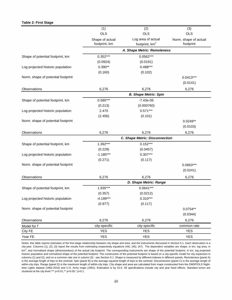
(1) (2) (3)

OLS OLS OLS

Shape of actual

footprint, km

Log area of actual

footprint, km2

Norm. shape of actual

footprint

Shape of potential footprint, km 0.352*** 0.0562***

(0.0924) (0.0191)

Log projected historic population 0.390** 0.488***

(0.160) (0.102)

Norm. shape of potential footprint 0.0413***

(0.0141)

Observations 6,276 6,276 6,276

Shape of potential footprint, km 0.585*** -7.43e-05

(0.213) (0.000760)

Log projected historic population 2.470 0.571***

(2.456) (0.101)

Norm. shape of potential footprint 0.0249**

(0.0103)

Observations 6,276 6,276 6,276

Shape of potential footprint, km 1.392*** 0.152***

(0.229) (0.0457)

Log projected historic population -1.180*** 0.307***

(0.271) (0.117)

Norm. shape of potential footprint 0.0663***

(0.0241)

Observations 6,276 6,276 6,276

Shape of potential footprint, km 1.935*** 0.0641***

(0.357) (0.0212)

Log projected historic population -4.199*** 0.310***

(0.977) (0.117)

Norm. shape of potential footprint 0.0754**

(0.0344)

Observations 6,276 6,276 6,276

Model for city-specific city-specific common rate

City FE YES YES YES

Year FE YES YES YES

Table 2: First Stage

Notes: this table reports estimates of the first-stage relationship between city shape and area, and the instruments discussed in Section 5.1. Each observation is a

city-year. Columns (1), (2), (3) report the results from estimating respectively equations (44), (45), (47). The dependent variables are shape, in km, log area, in

km2, and normalized shape (dimensionless) of the actual city footprint. The corresponding instruments are shape of the potential footprint, in km, log projected

historic population and normalized shape of the potential footprint. The construction of the potential footprint is based on a city-specific model for city expansion in

columns (1) and (2), and on a common rate one in column (3) - see Section 5.1. Shape is measured by different indexes in different panels. Remoteness (panel A)

is the average length of trips to the centroid. Spin (panel B) is the average squared length of trips to the centroid. Disconnection (panel C) is the average length of

within-city trips. Range (panel D) is the maximum length of within-city trips. City shape and area are calculated from maps constructed from the DMSP/OLS Night-

time Lights dataset (1992-2010) and U.S. Army maps (1951). Estimation is by OLS. All specifications include city and year fixed effects. Standard errors are

clustered at the city level.*** p<0.01,** p<0.05,* p<0.1.

A. Shape Metric: Remoteness

B. Shape Metric: Spin

C. Shape Metric: Disconnection

D. Shape Metric: Range

48

(1) (2) (3)

IV IV OLS

Log population Population density Log population

Shape of actual footprint, km -0.137** 0.0338***

(0.0550) (0.0112)

Log area of actual footprint, km2

0.785*** 0.167***

(0.182) (0.0318)

Norm. shape of actual footprint -311.8***

(92.18)

Observations 1,440 1,440 1,440

Shape of actual footprint, km -0.00101 0.000887***

(0.000657) (0.000288)

Log area of actual footprint, km2

0.547*** 0.197***

(0.101) (0.0290)

Norm. shape of actual footprint -110.9***

(37.62)

Observations 1,440 1,440 1,440

Shape of actual footprint, km -0.0991** 0.0249***

(0.0386) (0.00817)

Log area of actual footprint, km2

0.782*** 0.167***

(0.176) (0.0318)

Norm. shape of actual footprint -254.6***

(80.01)

Observations 1,440 1,440 1,440

Shape of actual footprint, km -0.0284*** 0.00763***

(0.0110) (0.00236)

Log area of actual footprint, km2

0.746*** 0.171***

(0.164) (0.0305)

Norm. shape of actual footprint -84.14***

(27.70)

Observations 1,440 1,440 1,440

Model for city-specific common rate

City FE YES YES YES

Year FE YES YES YES

Table 3: Impact of City Shape on Population

A. Shape Metric: Remoteness

B. Shape Metric: Spin

C. Shape Metric: Disconnection

D. Shape Metric: Range

Notes: this table reports estimates of the relationship between city shape and population. Each observation is a city-year. Column (1) reports the results from estimating

equation (43) (Specification I). The dependent variable is log city population. The explanatory variables are log city area, in km2, and city shape, in km. Column (2) reports

the results from estimating equation (46) (Specification II). The dependent variable is population density, in thousands of inhabitants per km2. The explanatory variable is

normalized shape (dimensionless). In columns (1) and (2) estimation is by IV. The instruments are discussed in Section 5.2, and the corresponding first-stage estimates are

reported in Table 2. The construction of the potential footprint is based on a city-specific model for city expansion in columns (1) and (2), and on a common rate one in

column (3) - see Section 5.1. Column (3) reports the same specification as column (1), estimated by OLS. Shape is measured by different indexes in different panels.

Remoteness (panel A) is the average length of trips to the centroid. Spin (panel B) is the average squared length of trips to the centroid. Disconnection (panel C) is the

average length of within-city trips. Range (panel D) is the maximum length of within-city trips. City shape and area are calculated from maps constructed from the

DMSP/OLS Night-time Lights dataset (1992-2010) and U.S. Army maps (1951). Population is drawn from the Census of India (1951, 1991, 2001, 2011). All specifications

include city and year fixed effects. Standard errors are clustered at the city level.*** p<0.01,** p<0.05,* p<0.1.

49

(1) (2) (3) (4) (5) (6)

FS(1) FS(2) IV FS(1) FS(2) IV

Shape of actual

footprint, km

Log area of actual

footprint, km2

Log population Shape of actual

footprint, km

Log area of actual

footprint, km2

Log population

Shape of potential

footprint, km 1.365*** 0.155*** 1.376*** 0.158***

(0.228) (0.0462) (0.233) (0.0488)

Log projected historic

population -1.201*** 0.278** -1.213*** 0.294**

(0.267) (0.118) (0.276) (0.123)

Shape of actual

footprint, km -0.100** -0.109**

(0.0414) (0.0428)

Log area of actual

footprint, km2

0.776*** 0.796***

(0.190) (0.185)

Observations 6,006 6,006 1,373 5,996 5,996 1,385

Cities 433 433 433 440 440 440

Sample excludes coastal cities coastal cities coastal cities mountainous cities mountainous cities mountainous cities

City FE YES YES YES YES YES YES

Year FE YES YES YES YES YES YES

Notes: this table presents a robustness check to Tables 2 and 3, excluding cities with “extreme” topographies from the sample. Each observation is a city-year. Columns (1), (2) and (4), (5) are equivalent to columns (1), (2)

in Table 1. They report OLS estimates of the first-stage relationship between city shape and area and the instruments discussed in Section 5.1. Columns (3) and (6) are equivalent to column (1) in Table 3, and report IV

estimates of the impact of shape on log city population. Shape is captured by the disconnection index, which measures the average length of trips within the city footprint, in km. The construction of the potential footprint is

based on a city-specific model for city expansion – see Section 5.1. Columns (1) to (3) exclude from the sample cities located within 5 km from the coast. Columns (4) to (6) exclude from the sample cities with an elevation

above 600 m. City shape and area are calculated from maps constructed from the DMSP/OLS Night-time Lights dataset (1992-2010) and U.S. Army maps (1951). Population is drawn from the Census of India (1951, 1991,

2001, 2011). Elevation is from the ASTER dataset. All specifications include city and year fixed effects. Standard errors are clustered at the city level. *** p<0.01,** p<0.05,* p<0.1.

Table 4: First Stage and Impact of City Shape on Population, Robustness to Excluding Cities with Extreme Topographies

50

(1) (2) (3) (4) (5) (6) (7) (8) (9)

IV IV OLS IV IV OLS IV IV OLS

Shape of actual

footprint, km 0.0381 0.109*** 0.0538*** 0.0626 0.0996*** 0.0586*** 0.0600* 0.112*** 0.0512***

(0.0386) (0.0275) (0.0172) (0.0536) (0.0336) (0.0150) (0.0360) (0.0300) (0.0181)

Log area of actual

footprint, km2 -0.409 -0.0478 -0.167 -0.00936 -0.337 -0.0308

(0.390) (0.0356) (0.465) (0.0516) (0.392) (0.0478)

Observations 2,009 2,009 2,009 1,075 1,075 1,075 1,517 1,517 1,517

Model for city-specific common rate city-specific common rate city-specific common rate

City FE YES YES YES YES YES YES YES YES YES

Year FE YES YES YES YES YES YES YES YES YES

Table 5: Impact of City Shape on Wages

Notes: this table reports estimates of relationship between city shape and average wages. Each observation is a city-year. The dependent variable is the log urban average of individual yearly wages in the city’s district, in thousand 2014

Rupees. The explanatory variables are log city area, in km2, and city shape, in km. Columns (1), (4), (7) report the results from estimating equation (43) (Specification I) by IV. Columns (3), (6), (9) report the same specification, estimated

by OLS. Columns (2), (5), (8) report the results from estimating equation (48) (Specification II) by IV. Instruments are described in Section 5.2. The construction of the potential footprint is based on a city-specific model for city expansion

in columns (1), (4) and (7), and on a common rate one in column (2), (5), (8) – see Section 5.1. In columns (4), (5), (6) the sample is restricted to districts containing only one city. In columns (7), (8), (9) the sample is restricted to cities

which are either the only ones or the top ones in their respective districts. Shape is captured by the disconnection index, which measures the average length of trips within the city footprint, in km. City shape and area are calculated from

maps constructed from the DMSP/OLS Night-time Lights dataset (1992-2010). Wages are from the Annual Survey of Industries, waves 1990, 1994, 1995, 1997, 1998, 2009, 2010. All specifications include city and year fixed effects.

Standard errors are clustered at the city level. *** p<0.01,** p<0.05,* p<0.1.

Dependent variable: log wage

All districts Only districts with one city Only top city per district

51

(1) (2) (3) (4) (5) (6) (7) (8) (9)

IV IV OLS IV IV OLS IV IV OLS

Shape of actual

footprint, km-0.596 -0.303 0.00204 -0.518* -0.636 -0.00857 -0.684 -0.198 0.0107

(0.396) (0.758) (0.0505) (0.285) (1.661) (0.0736) (0.538) (0.806) (0.0516)

Log area of actual

footprint, km2 -1.529 -0.0176 -0.919 -0.0632 -1.407 -0.0355

(1.409) (0.0847) (0.870) (0.108) (1.582) (0.0962)

Observations 895 895 895 476 476 476 711 711 711

Shape of actual

footprint, km-0.675 -0.274 -0.00526 -0.594* -0.595 -0.00736 -0.790 -0.143 0.00685

(0.432) (0.752) (0.0577) (0.324) (1.626) (0.0825) (0.604) (0.780) (0.0590)

Log area of actual

footprint, km2 -1.649 -0.00333 -1.040 -0.0485 -1.586 -0.0141

(1.542) (0.0976) (0.990) (0.125) (1.786) (0.110)

Observations 895 895 895 476 476 476 711 711 711

Model for city-specific common rate city-specific common rate city-specific common rate

City FE YES YES YES YES YES YES YES YES YES

Year FE YES YES YES YES YES YES YES YES YES

Notes: this table reports estimates of relationship between city shape and average housing rents. Each observation is a city-year. In panel A the dependent variable is the log urban average of housing rent per m2

in the city’s district, in

2014 Rupees. In panel B the dependent variable is analogous, but the average is calculated considering only the top 50% of the district’s distribution of rents per m2. The explanatory variables are log city area, in km2, and city shape, in

km. Columns (1), (4), (7) report the results from estimating equation (43) (Specification I) by IV. Columns (3), (6), (9) report the same specification, estimated by OLS. Columns (2), (5), (8) report the results from estimating equation (48)

(Specification II) by IV. Instruments are described in Section 5.2. The construction of the potential footprint is based on a city-specific model for city expansion in columns (1), (4) and (7), and on a common rate one in column (2), (5), (8)

– see Section 5.1. In columns (4), (5), (6) the sample is restricted to districts containing only one city. In columns (7), (8), (9) the sample is restricted to cities which are either the only ones or the top ones in their respective districts.

Shape is captured by the disconnection index, which measures the average length of trips within the city footprint, in km. City shape and area are calculated from maps constructed from the DMSP/OLS Night-time Lights dataset (1992-

2010). Housing rents are from the NSS Household Consumer Expenditure Survey, rounds 62 (2005-2006), 63 (2006-2007) and 64 (2007-2008). All specifications include city and year fixed effects. Standard errors are clustered at the

city level. *** p<0.01,** p<0.05,* p<0.1.

B. Dependent variable: log yearly rent per square meter, upper 50%

Table 6: Impact of City Shape on Housing Rents

All districts Only districts with one city Only top city per district

A. Dependent variable: log yearly rent per square meter

52

(1) (2) (3) (4) (5) (6)

IV IV IV IV IV IV

Norm. shape -183.9*** -48.25*** -103.9*** -30.34*** -140.5*** -37.71***

(39.53) (9.047) (18.10) (5.485) (44.85) (9.934)

Norm. shape x

state motor vehicles density, 1991 0.0462*** 0.0246***

(0.0179) (0.00441)

Norm. shape x

urban road density, 1991 0.204*** 0.0692***

(0.0204) (0.00776)

Norm. shape x

state urban road density, 1991 0.000462 0.000207*

(0.000312) (0.000107)

Observations 1,286 1,286 1,406 1,406 1,380 1,380

Shape metric disconnection range disconnection range disconnection range

City FE YES YES YES YES YES YES

Year FE YES YES YES YES YES YES

Notes: this table investigates the impact of shape, interacted with infrastructure, on population. Each observation is a city-year. All columns report IV estimates of a specification similar to equation (46) (Specification II),

augmented with an interaction between normalized shape and different infrastructure proxies. The dependent variable is population density, in thousands of inhabitants per km2. The construction of the potential footprint is

based on a city-specific model for city expansion – see Section 5.1. The shape metrics considered are the normalized disconnection index (columns (1), (3), (5)), and normalized range index (columns (2), (4), (6)).

Disconnection is the average length of within-city trips. Range is the maximum length of within-city trips. In columns (1), (2) normalized shape is interacted with state motor vehicles density in 1991 (source: Ministry of Road

Transport and Highways). In columns (3), (4) normalized shape is interacted with urban road density in the city, as reported in the 1991 Census. In columns (4), (5) normalized shape is interacted with a leave-out mean of

urban road density in the state calculated using 1991 Census data and data from the Ministry of Road Transport and Highways .City shape and area are calculated from maps constructed from the DMSP/OLS Night-time

Lights dataset (1992-2010) and U.S. Army maps (1951). Population is drawn from the Census of India (1951, 1991, 2001, 2011). All specifications include city and year fixed effects. Standard errors are clustered at the city

level. *** p<0.01,** p<0.05,* p<0.1.

Table 7: Interactions of City Shape with Infrastructure

Dependent variable: population density

53

(1) (2) (3) (4) (5) (6) (7) (8) (9)

IV IV OLS IV IV OLS IV IV OLS

Shape of actual

footprint, km -0.134** -0.0431 -0.0353** -0.113** -0.0501*** -0.0498*** 0.195* 0.174* -0.00698

(0.0540) (0.0437) (0.0167) (0.0561) (0.0185) (0.0169) (0.118) (0.0940) (0.0312)

Log area of actual

footprint, km2

0.592 0.134 0.264 0.0501 0.438 0.141

(0.492) (0.0829) (0.633) (0.0938) (1.483) (0.120)

Observations 1,067 1,067 1,067 1,067 1,067 1,067 822 822 822

Model for city-specific common rate city-specific common rate city-specific common rate

City FE YES YES YES YES YES YES YES YES YES

Year FE YES YES YES YES YES YES YES YES YES

Table 8: Impact of City Shape on Housing Quality

Notes: this table reports estimates of relationship between city shape and proxies for housing quality. Each observation is a city-year. Columns (1), (4), (7) report the results from estimating equation (43) (Specification I) by IV.

Columns (3), (6), (9) report the same specification, estimated by OLS. Columns (2), (5), (8) report the results from estimating equation (48) (Specification II) by IV. The explanatory variables are shape, in km, and log city area, in

km2. Instruments are described in Section 5.2. The construction of the potential footprint is based on a city-specific model for city expansion in columns (1), (4) and (7), and on a common rate one in column (2), (5), (8) – see

Section 5.1. The dependent variables are the following: log slum population in the city (columns (1), (2), (3)), log of the share of slum to total population in the city (columns (4), (5), (6)), and a housing quality principal component

index (columns (7), (8), (9)). Data on slums are drawn from the 1991, 2001 and 2011 Census. The housing quality index is the city-year average of a principal component index based on the following characteristics of Census

houses: roof, wall and floor material, availability of running water and toilet in-premise. The source is the 2001 and 2011 Census. Shape is captured by the disconnection index, which measures the average length of trips within

the city footprint, in km. City shape and area are calculated from maps constructed from the DMSP/OLS Night-time Lights dataset (1992-2010). All specifications include city and year fixed effects. Standard errors are clustered at

the city level. *** p<0.01,** p<0.05,* p<0.1.

Log slum population shareLog slum population Housing index

54

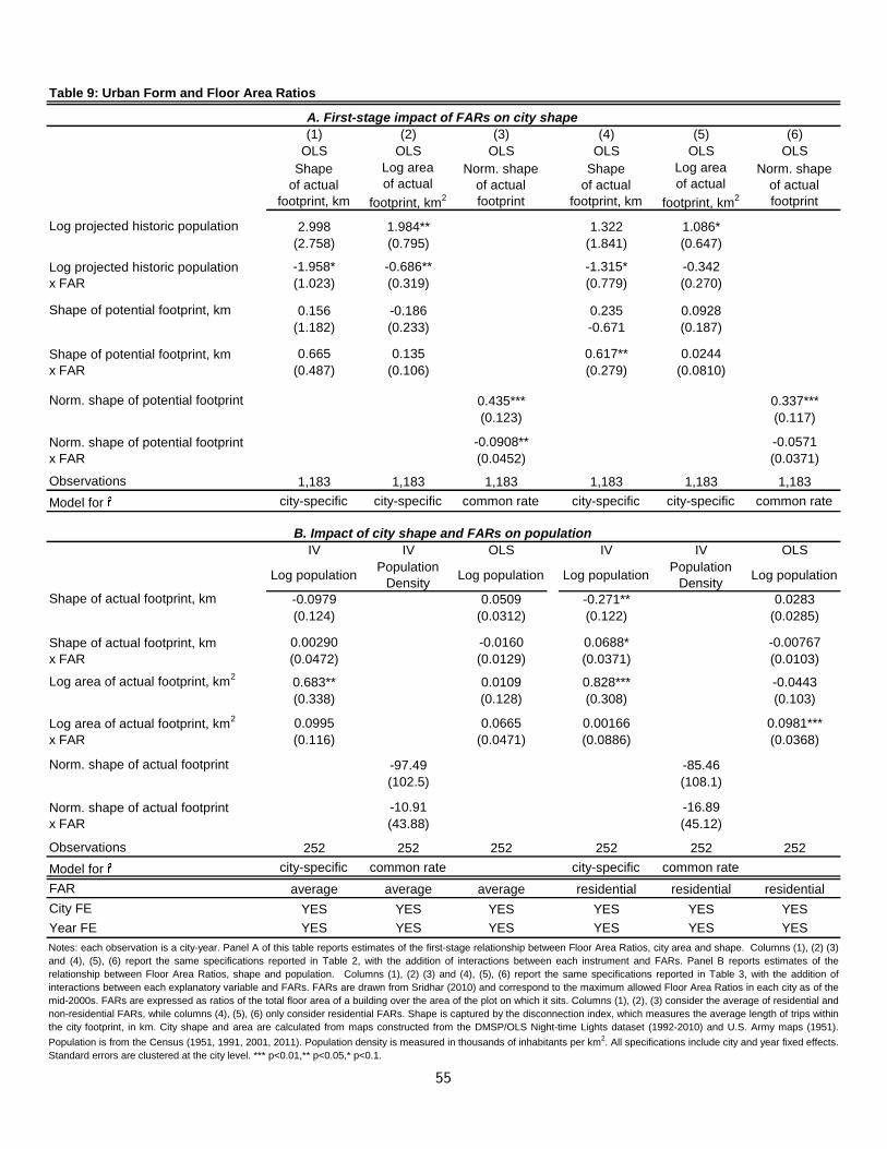
(1) (2) (3) (4) (5) (6)

OLS OLS OLS OLS OLS OLS

Shape

of actual

footprint, km

Log area

of actual

footprint, km2

Norm. shape

of actual

footprint

Shape

of actual

footprint, km

Log area

of actual

footprint, km2

Norm. shape

of actual

footprint

Log projected historic population 2.998 1.984** 1.322 1.086*

(2.758) (0.795) (1.841) (0.647)

-1.958* -0.686** -1.315* -0.342

(1.023) (0.319) (0.779) (0.270)

Shape of potential footprint, km 0.156 -0.186 0.235 0.0928

(1.182) (0.233) -0.671 (0.187)

0.665 0.135 0.617** 0.0244

(0.487) (0.106) (0.279) (0.0810)

Norm. shape of potential footprint 0.435*** 0.337***

(0.123) (0.117)

-0.0908** -0.0571

(0.0452) (0.0371)

Observations 1,183 1,183 1,183 1,183 1,183 1,183

Model for city-specific city-specific common rate city-specific city-specific common rate

IV IV OLS IV IV OLS

Log populationPopulation

DensityLog population Log population

Population

DensityLog population

Shape of actual footprint, km -0.0979 0.0509 -0.271** 0.0283

(0.124) (0.0312) (0.122) (0.0285)

0.00290 -0.0160 0.0688* -0.00767

(0.0472) (0.0129) (0.0371) (0.0103)

Log area of actual footprint, km2

0.683** 0.0109 0.828*** -0.0443

(0.338) (0.128) (0.308) (0.103)

0.0995 0.0665 0.00166 0.0981***

(0.116) (0.0471) (0.0886) (0.0368)

Norm. shape of actual footprint -97.49 -85.46

(102.5) (108.1)

-10.91 -16.89

(43.88) (45.12)

Observations 252 252 252 252 252 252

Model for city-specific common rate city-specific common rate

FAR average average average residential residential residential

City FE YES YES YES YES YES YES

Year FE YES YES YES YES YES YES

Norm. shape of actual footprint

x FAR

Notes: each observation is a city-year. Panel A of this table reports estimates of the first-stage relationship between Floor Area Ratios, city area and shape. Columns (1), (2) (3)

and (4), (5), (6) report the same specifications reported in Table 2, with the addition of interactions between each instrument and FARs. Panel B reports estimates of the

relationship between Floor Area Ratios, shape and population. Columns (1), (2) (3) and (4), (5), (6) report the same specifications reported in Table 3, with the addition of

interactions between each explanatory variable and FARs. FARs are drawn from Sridhar (2010) and correspond to the maximum allowed Floor Area Ratios in each city as of the

mid-2000s. FARs are expressed as ratios of the total floor area of a building over the area of the plot on which it sits. Columns (1), (2), (3) consider the average of residential and

non-residential FARs, while columns (4), (5), (6) only consider residential FARs. Shape is captured by the disconnection index, which measures the average length of trips within

the city footprint, in km. City shape and area are calculated from maps constructed from the DMSP/OLS Night-time Lights dataset (1992-2010) and U.S. Army maps (1951).

Population is from the Census (1951, 1991, 2001, 2011). Population density is measured in thousands of inhabitants per km2. All specifications include city and year fixed effects.

Standard errors are clustered at the city level. *** p<0.01,** p<0.05,* p<0.1.

Table 9: Urban Form and Floor Area Ratios

B. Impact of city shape and FARs on population

A. First-stage impact of FARs on city shape

Shape of potential footprint, km

x FAR

Log projected historic population

x FAR

Norm. shape of potential footprint

x FAR

Shape of actual footprint, km

x FAR

Log area of actual footprint, km2

x FAR

55

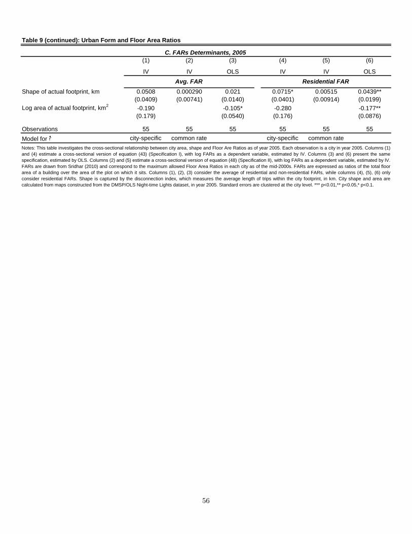
(1) (2) (3) (4) (5) (6)

IV IV OLS IV IV OLS

Shape of actual footprint, km 0.0508 0.000290 0.021 0.0715* 0.00515 0.0439**

(0.0409) (0.00741) (0.0140) (0.0401) (0.00914) (0.0199)

Log area of actual footprint, km2

-0.190 -0.105* -0.280 -0.177**

(0.179) (0.0540) (0.176) (0.0876)

Observations 55 55 55 55 55 55

Model for city-specific common rate city-specific common rate

Notes: This table investigates the cross-sectional relationship between city area, shape and Floor Are Ratios as of year 2005. Each observation is a city in year 2005. Columns (1)

and (4) estimate a cross-sectional version of equation (43) (Specification I), with log FARs as a dependent variable, estimated by IV. Columns (3) and (6) present the same

specification, estimated by OLS. Columns (2) and (5) estimate a cross-sectional version of equation (48) (Specification II), with log FARs as a dependent variable, estimated by IV.

FARs are drawn from Sridhar (2010) and correspond to the maximum allowed Floor Area Ratios in each city as of the mid-2000s. FARs are expressed as ratios of the total floor

area of a building over the area of the plot on which it sits. Columns (1), (2), (3) consider the average of residential and non-residential FARs, while columns (4), (5), (6) only

consider residential FARs. Shape is captured by the disconnection index, which measures the average length of trips within the city footprint, in km. City shape and area are

calculated from maps constructed from the DMSP/OLS Night-time Lights dataset, in year 2005. Standard errors are clustered at the city level. *** p<0.01,** p<0.05,* p<0.1.

Avg. FAR Residential FAR

Table 9 (continued): Urban Form and Floor Area Ratios

C. FARs Determinants, 2005

56

(1) (2) (3) (4) (5) (6)

IV IV OLS IV IV OLS

Log road length, km Road density, km/km2 Log road length, km Log road length, km Road density, km/km

2 Log road length, km

Shape of actual footprint, km -0.0769* 0.0231** -0.0237** 0.00655**

(0.0429) (0.0111) (0.0109) (0.00320)

Log area of actual footprint, km2

1.292*** 0.861*** 1.279*** 0.871***

(0.147) (0.0415) (0.115) (0.0379)

Norm. shape of actual footprint 9.131 -3.563

(16.44) (3.816)

Observations 429 429 429 429 429 429

Log road length

per capita

Road density

per capita

Log road length

per capita

Log road length

per capita

Road density

per capita

Log road length

per capita

Shape of actual footprint, km 0.0403 -0.0677*** 0.00753 -0.0190***

(0.0467) (0.0149) (0.0111) (0.00427)

Log area of actual footprint, km2

-0.201 0.346*** -0.143 0.317***

(0.178) (0.0597) (0.138) (0.0547)

Norm. shape of actual footprint -0.0377 -0.0152

(0.0785) (0.0211)

Observations 429 429 429 429 429 429

Model for city-specific common rate city-specific common rate

Shape metric disconnection disconnection disconnection range range range

Notes: This table estimates the cross-sectional relationship between city area, shape and road network as of year 2010. Panel A considers total road length and panel B considers road length per capita. Each observation is a city in year

2010. Columns (1) and (4) estimate a cross-sectional version of equation (43) (Specification I), estimated by IV. Columns (3) and (6) present the same specification, estimated by OLS. In columns (1), (3), (4), (6), panel A, the dependent

variable is log road length in the footprint, in km. In columns (1), (3), (4), (6), panel B, the dependent variable is log road length per capita in the footprint, in km per thousand inhabitants. Columns (2) and (5) estimate a cross-sectional

version of equation (46) (Specification II), estimated by IV. In columns (2), (5), panel A, the dependent variable is road density in the footprint, in km per km2. In columns (2), (5) panel B, the dependent variable is road density per capita,

in in km per km2

per thousand inhabitants. The construction of the potential footprint is based on a city-specific model for city expansion in columns (1) and (4), and on a common rate on in columns (2) and (5) – see Section 5.1. Road

length is computed based on current (2014) Openstreetmap maps of Indian cities, focusing on roads denoted as “trunk”, “primary” or “secondary”. Disconnection is the average length of trips within the city footprint, in km. Range is the

longest possible within-footprint trip, in km. City shape and area are calculated from maps constructed from the DMSP/OLS Night-time Lights dataset, in year 2010. Standard errors are clustered at the city level. *** p<0.01,** p<0.05,*

p<0.1.

A. Total Roads

B. Roads per capita

Table 10: Impact of City Shape on Road Network, 2010

57

(1) (2) (3) (4) (5) (6)

IV IV OLS IV IV OLS

Shape of actual footprint, km -0.198** -0.00633 -0.0410** -0.000758

(0.0978) (0.0248) (0.0182) (0.00673)

Log area of actual footprint, km2

0.395** 0.0519 0.244** 0.0449

(0.181) (0.0498) (0.0958) (0.0403)

Norm. shape of actual footprint 22.33 -1.117

(103.1) (1.345)

Observations 196 196 196 196 196 196

Model for city-specific common rate city-specific common rate

Shape metric disconnection disconnection disconnection range range range

Dependent variable: Moran's I index of spatial concentration

Table 11: Impact of City Shape on the Spatial Distribution of Productive Establishments, 2005

Notes: This table investigates the cross-sectional relationship between city area, shape and the spatial concentration of productive establishments in cities as of year 2005. Each observation is a

city in year 2005. The dependent variable is the Moran’s I index of spatial concentration, computed in each city for the location of productive establishments, as reported in the urban directories of

the 2005 Economic Census. Higher values indicate more spatial clustering. Columns (1) and (4) estimate a cross-sectional version of equation (43) (Specification I), estimated by IV. Columns (3)

and (6) present the same specification, estimated by OLS. Columns (2) and (5) estimate a cross-sectional version of equation (48) (Specification II), estimated by IV. The construction of the

potential footprint is based on a city-specific model for city expansion in columns (1) and (3), and on a common rate on in columns (2) and (4) – see Section 5.1. The shape metrics considered are

the disconnection index (columns (1), (2), (3)), and range index (columns (4), (5), (6)). Disconnection is the average length of trips within the city footprint, in km. Range is the longest possible

within-footprint trip, in km. City shape and area is calculated from maps constructed from the DMSP/OLS Night-time Lights dataset, in year 2005. Standard errors are clustered at the city level. ***

p<0.01,** p<0.05,* p<0.1

58

(1) (2)

IV IV

Log population Population density

Shape of actual footprint, km -0.194***

(0.0596)

Log area of actual footprint, km2

0.973***

(0.222)

Norm. shape of actual footprint -254.6***

(80.01)

Observations 1,440 1,440

Model for city-specific common rate

City FE YES YES

Year FE YES YES

Initial shape x year FE YES YES

Appendix Table 1: Impact of Shape on Population, Robustness to Initial Shape x Year Fixed Effects

Notes: this table presents a robustness check to Table 3, augmenting the specification with year fixed effects interacted with initial shape. Each

observation is a city-year. Columns (1) and (2) are equivalent to columns (1) and (2) in Table 3. They report IV estimates of the relationship between

city shape and area and log city population (col. 1) and population density, in thousand inhabitants per km2

(col.2). Shape is captured by the

disconnection index, which measures the average length of trips within the city footprint, in km. The construction of the potential footprint is based

on a city-specific model for city expansion in column (1) and on a common rate on in column (2) – see Section 5.1. City shape and area are

calculated from maps constructed from the DMSP/OLS Night-time Lights dataset (1992-2010) and U.S. Army maps (1951). Population is drawn

from the Census of India (1951, 1991, 2001, 2011). All specifications include city and year fixed effects, as well as year fixed effects interacted with

the city’s disconnection index measured in the initial year of the panel (1951). Standard errors are clustered at the city level. *** p<0.01,** p<0.05,*

p<0.1.

59

(1) (2) (3) (4) (5) (6)

IV IV IV IV IV IV

Shape of actual footprint, km 0.0116 0.0989*** 0.0393 0.108** 0.0381 0.102***

(0.0420) (0.0272) (0.0768) (0.0421) (0.0386) (0.0298)

Log area of actual footprint, km2 -0.358 -0.164 -0.274

(0.395) (0.465) (0.379)

Observations 2,009 2,009 1,075 1,075 1,517 1,517

Shape of actual footprint, km -0.739 -0.393* -0.670* -0.465* -0.839 -0.447*

(0.487) (0.221) (0.359) (0.265) (0.664) (0.251)

Log area of actual footprint, km2 -1.301 -0.619 -1.092

(1.355) (0.807) (1.444)

Observations 896 896 477 477 712 712

City FE YES YES YES YES YES YES

Year FE YES YES YES YES YES YES

Initial shape x year FE YES YES YES YES YES YES

Model for city-specific common rate city-specific common rate city-specific common rate

Appendix Table 2: Impact of Shape on Wages and Rents, Robustness to Initial Shape x Year Fixed Effects

All districts Only districts with one city Only top city per district

A. Dependent variable: log wage

Notes: this table presents a robustness check to Tables 5 and 6, augmenting the specifications with year fixed effects interacted with initial shape. Each observation is a city-year. In panel A the

dependent variable is the log urban average of individual yearly wages in the city’s district, in thousand 2014 Rupees. In panel B the dependent variable is the log urban average of housing rent

per m2

in the city’s district, in 2014 Rupees. Columns (1), (3), (5) report the results from estimating equation (43) (Specification I) by IV. Columns (2), (4), (6) report the results from estimating

equation (48) (Specification II) by IV. Instruments are described in Section 5.2. The construction of the potential footprint is based on a city-specific model for city expansion in columns (1), (3),

(5), and on a common rate one in column (2), (4), (6) – see Section 5.1. In columns (3), (4) the sample is restricted to districts containing only one city. In columns (5), (6) the sample is

restricted to cities which are either the only ones or the top ones in their respective districts. Shape is captured by the disconnection index, which measures the average length of trips within the

city footprint, in km. City shape and area are calculated from maps constructed from the DMSP/OLS Night-time Lights dataset (1992-2010). Wages are from the Annual Survey of Industries,

waves 1990, 1994, 1995, 1997, 1998, 2009, 2010. Housing rents are from the NSS Household Consumer Expenditure Survey, rounds 62 (2005-2006), 63 (2006-2007) and 64 (2007-2008). All

specifications include city and year fixed effects, as well as year fixed effects interacted with the city’s disconnection index measured in the initial year of the panel (1951). Standard errors are

clustered at the city level. *** p<0.01,** p<0.05,* p<0.1.

B. Dependent variable: log yearly rent per square meter

60

Figure 1:

U.S. Army India and Pakistan Topographic Maps

61

Figure 2

DMS/OLS nighttime lights, year 1992, luminosity threshold : 40.

62

Figure 3

Developable vs. constrained land

63

constrained developable

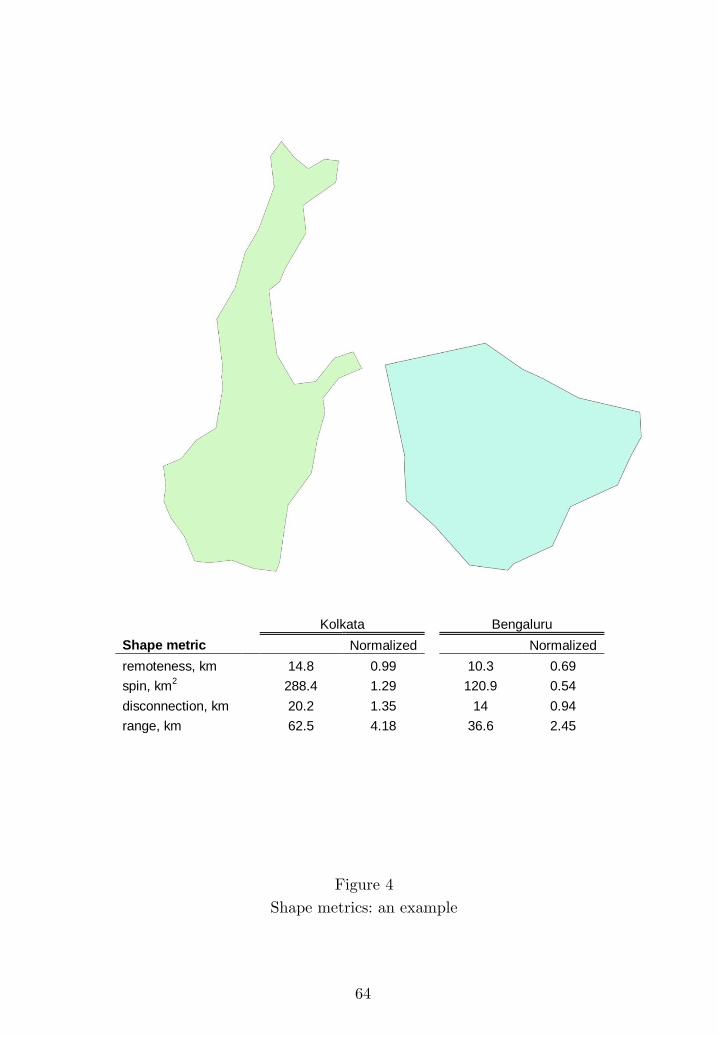
Figure 4

Shape metrics: an example

64

Kolkata

Bengaluru

Shape metric Normalized

Normalized

remoteness, km

14.8 0.99

10.3 0.69

spin, km2

288.4 1.29

120.9 0.54

disconnection, km

20.2 1.35

14 0.94

range, km

62.5 4.18

36.6 2.45

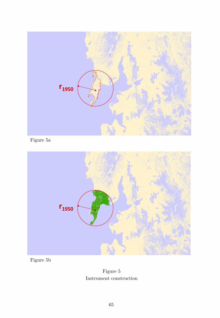
Figure 5

Instrument construction

65

Figure 5a

Figure 5b

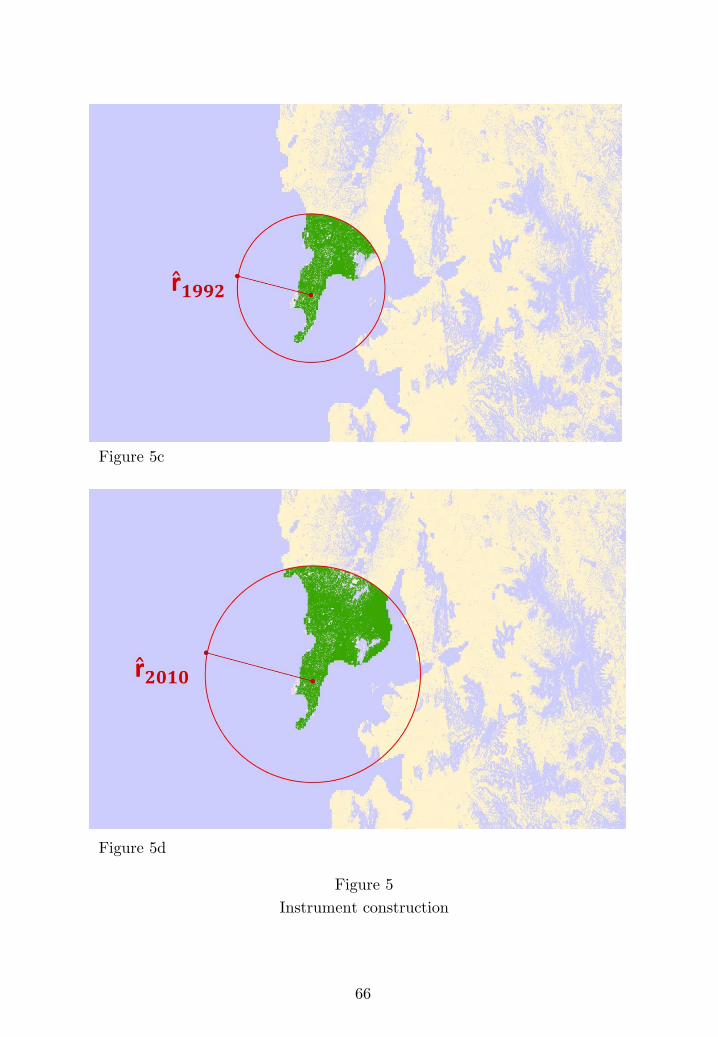
Figure 5

Instrument construction

66

Figure 5c

Figure 5d