city college of new york 1 dr. jizhong xiao department of electrical engineering city college of new...
TRANSCRIPT
1City College of New York
Dr. Jizhong Xiao
Department of Electrical Engineering
City College of New York
Advanced Mobile Robotics
Probabilistic Robotics (II)
2City College of New York
Outline
• Localization Methods– Markov Localization (review)– Kalman Filter Localization– Particle Filter (Monte Carlo Localization)
• Current Research Topics– SLAM – Multi-robot Localization
3City College of New York
Robot Navigation
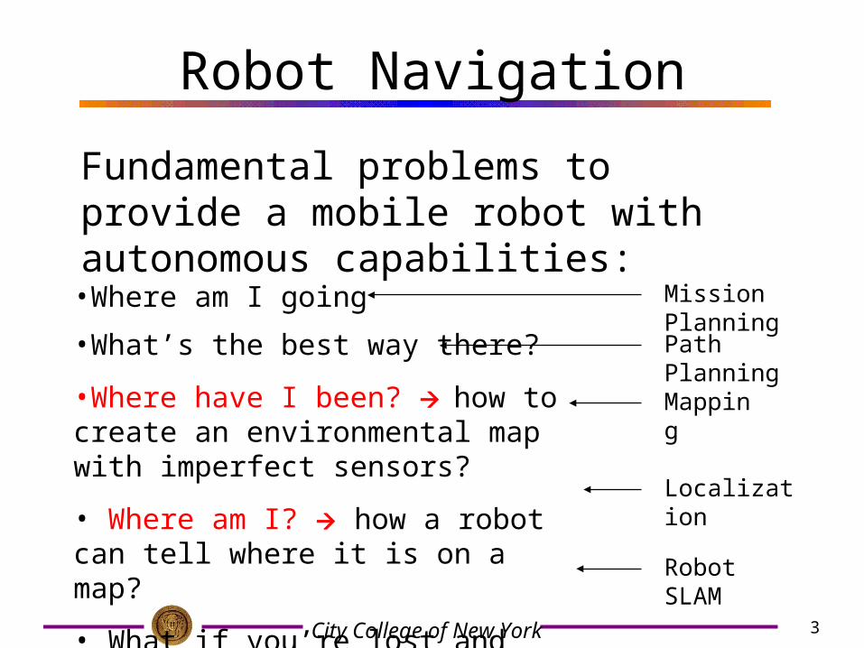
Fundamental problems to provide a mobile robot with autonomous capabilities:
•Where am I going
•What’s the best way there?
•Where have I been? how to create an environmental map with imperfect sensors?
• Where am I? how a robot can tell where it is on a map?
• What if you’re lost and don’t have a map?
Mapping
Localization
Robot SLAM
Path Planning
Mission Planning
4City College of New York
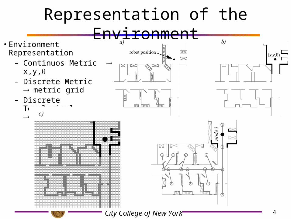
Representation of the Environment• Environment Representation
– Continuos Metric x,y,
– Discrete Metricmetric grid
– Discrete Topologicaltopological grid
5City College of New York
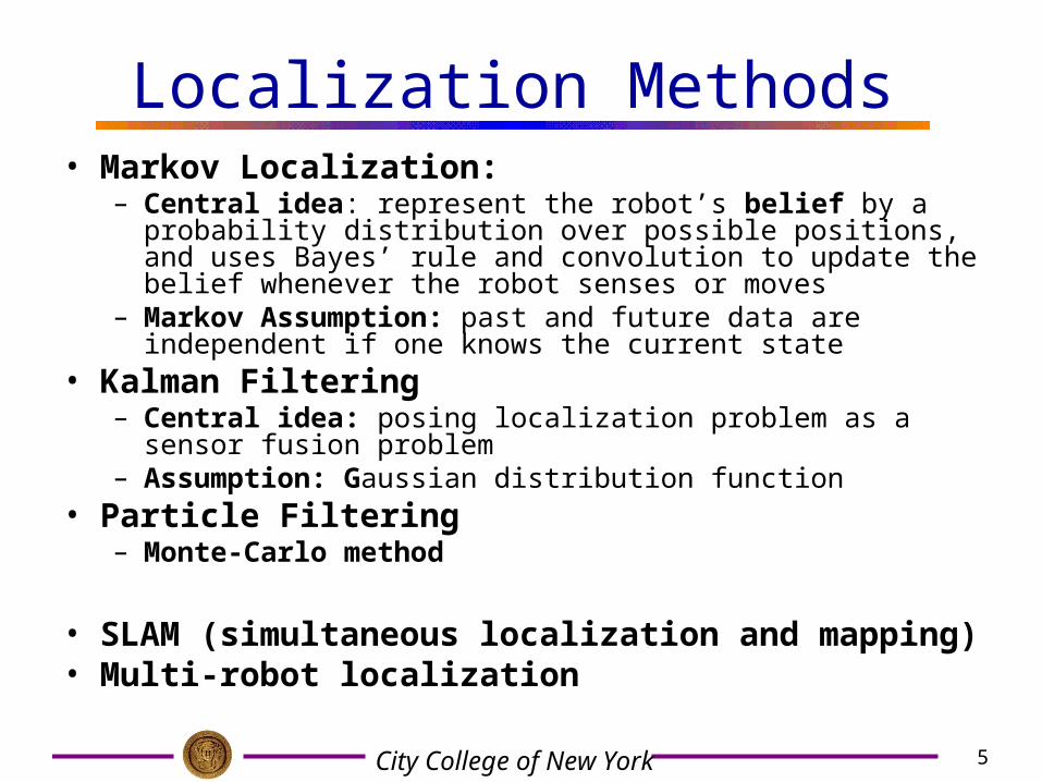
Localization Methods• Markov Localization:
– Central idea: represent the robot’s belief by a probability distribution over possible positions, and uses Bayes’ rule and convolution to update the belief whenever the robot senses or moves
– Markov Assumption: past and future data are independent if one knows the current state
• Kalman Filtering– Central idea: posing localization problem as a sensor fusion problem– Assumption: Gaussian distribution function
• Particle Filtering– Monte-Carlo method
• SLAM (simultaneous localization and mapping)• Multi-robot localization
6City College of New York
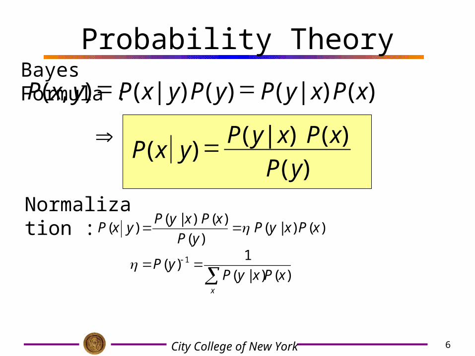
Probability TheoryBayes Formula :
)()|()()|(),(
)(
)()|()(
yP
xPxyPyxP
xPxyPyPyxPyxP
)()|(
1)(
)()|()(
)()|()(
1
xPxyPyP
xPxyPyP
xPxyPyxP
x
Normalization :
7City College of New York
Probability Theory
)|(
)|(),|(),|(
zyP
zxPzxyPzyxP
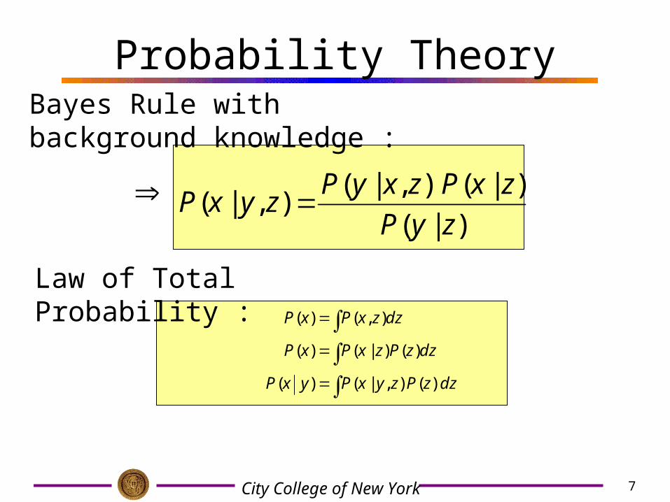
Bayes Rule with background knowledge :
dzzPzyxPyxP
dzzPzxPxP
dzzxPxP
)(),|()(
)()|()(
),()(
Law of Total Probability :
8City College of New York
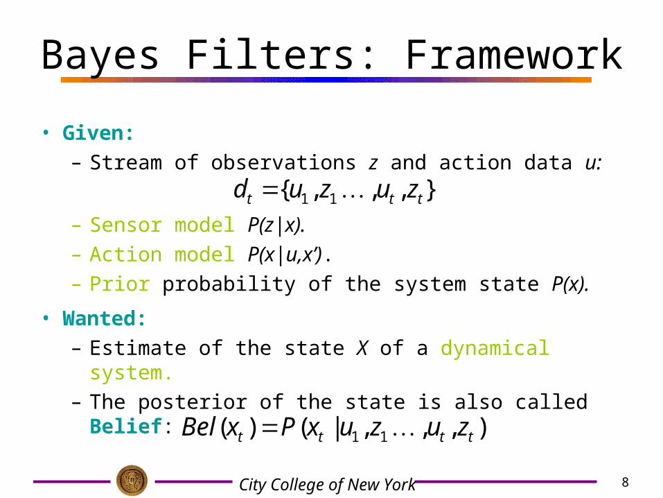
Bayes Filters: Framework
• Given:– Stream of observations z and action data u:
– Sensor model P(z|x).– Action model P(x|u,x’).– Prior probability of the system state P(x).
• Wanted: – Estimate of the state X of a dynamical system.– The posterior of the state is also called Belief:
),,,|()( 11 tttt zuzuxPxBel
},,,{ 11 ttt zuzud
9City College of New York
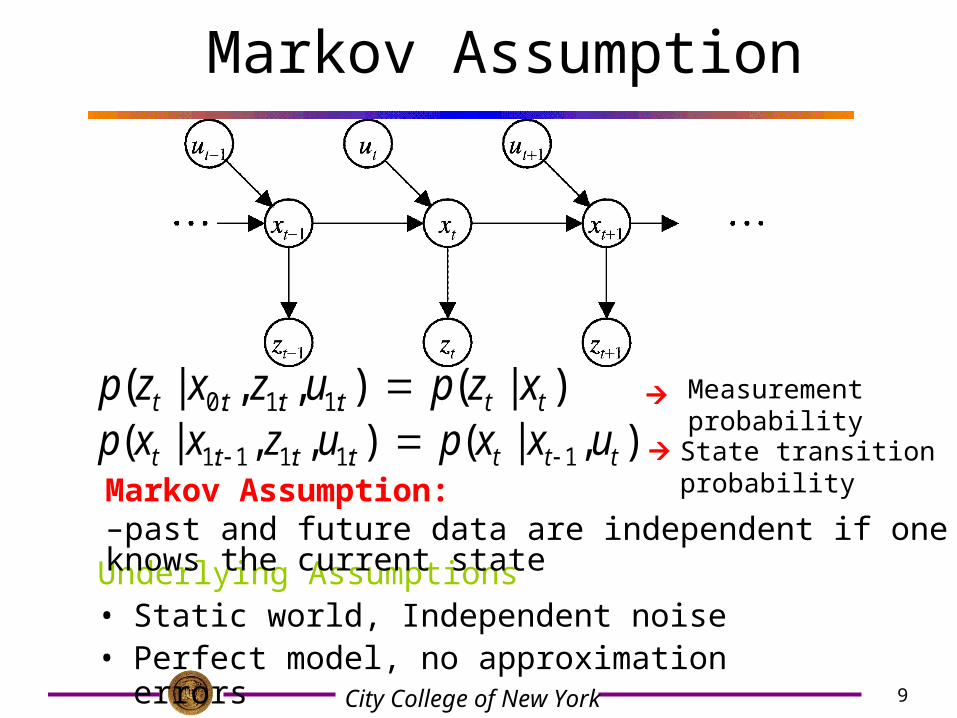
Markov Assumption
Underlying Assumptions• Static world, Independent noise• Perfect model, no approximation errors
),|(),,|( 1:1:11:1 ttttttt uxxpuzxxp )|(),,|( :1:1:0 tttttt xzpuzxzp
State transition probability
Measurement probability
Markov Assumption: –past and future data are independent if one knows the current state
10City College of New York
111 )(),|()|( ttttttt dxxBelxuxPxzP
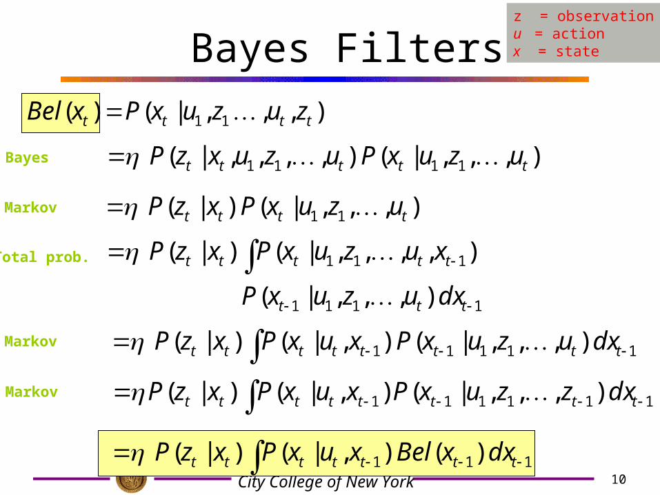
Bayes Filters
),,,|(),,,,|( 1111 ttttt uzuxPuzuxzP Bayes
z = observationu = actionx = state
),,,|()( 11 tttt zuzuxPxBel
Markov ),,,|()|( 11 tttt uzuxPxzP
Markov11111 ),,,|(),|()|( tttttttt dxuzuxPxuxPxzP
1111
111
),,,|(
),,,,|()|(
ttt
ttttt
dxuzuxP
xuzuxPxzP
Total prob.
Markov111111 ),,,|(),|()|( tttttttt dxzzuxPxuxPxzP
11City College of New York
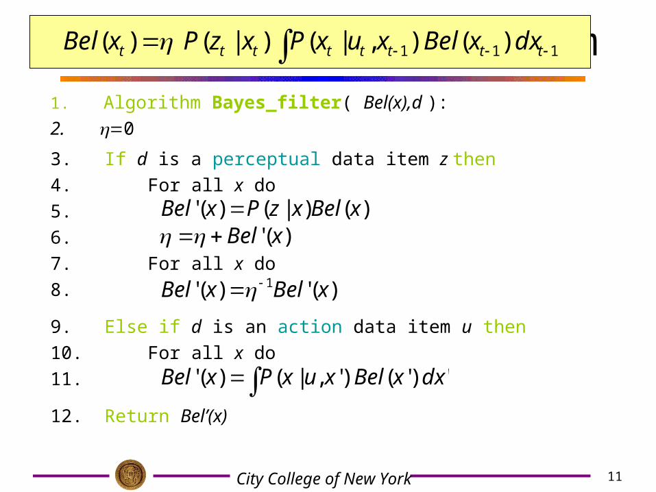
Bayes Filter Algorithm 1. Algorithm Bayes_filter( Bel(x),d ):
2. 0
3. If d is a perceptual data item z then
4. For all x do
5.
6.
7. For all x do
8.
9. Else if d is an action data item u then
10. For all x do
11.
12. Return Bel’(x)
)()|()(' xBelxzPxBel )(' xBel
)(')(' 1 xBelxBel
')'()',|()(' dxxBelxuxPxBel
111 )(),|()|()( tttttttt dxxBelxuxPxzPxBel
12City College of New York
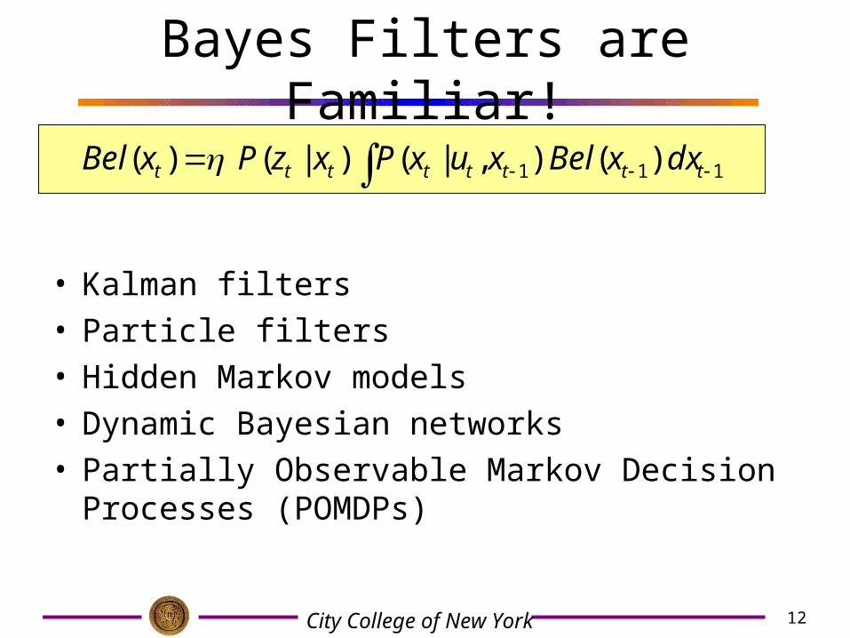
Bayes Filters are Familiar!
• Kalman filters• Particle filters• Hidden Markov models• Dynamic Bayesian networks• Partially Observable Markov Decision Processes
(POMDPs)
111 )(),|()|()( tttttttt dxxBelxuxPxzPxBel
13City College of New York
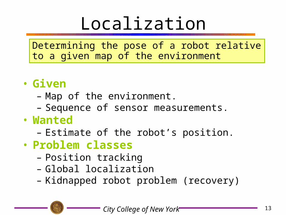
Localization
• Given – Map of the environment.– Sequence of sensor measurements.
• Wanted– Estimate of the robot’s position.
• Problem classes– Position tracking– Global localization– Kidnapped robot problem (recovery)
Determining the pose of a robot relative to a given map of the environment
14City College of New York
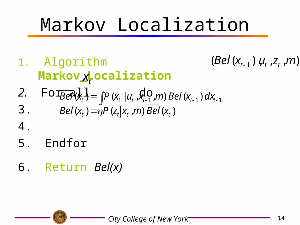
Markov Localization
1. Algorithm Markov_Localization
2. For all do
3.
4.
5. Endfor
6. Return Bel(x)
),,),(( 1 mzuxBel ttt
111 )(),,|()( tttttt dxxBelmxuxPxBel
)(),()( tttt xBelmxzPxBel
tx

15City College of New York

16City College of New York
Localization Methods• Markov Localization:
– Central idea: represent the robot’s belief by a probability distribution over possible positions, and uses Bayes’ rule and convolution to update the belief whenever the robot senses or moves
– Markov Assumption: past and future data are independent if one knows the current state
• Kalman Filtering– Central idea: posing localization problem as a sensor fusion problem– Assumption: Gaussian distribution function
• Particle Filtering– Monte-Carlo method
• SLAM (simultaneous localization and mapping)• Multi-robot localization
17City College of New York
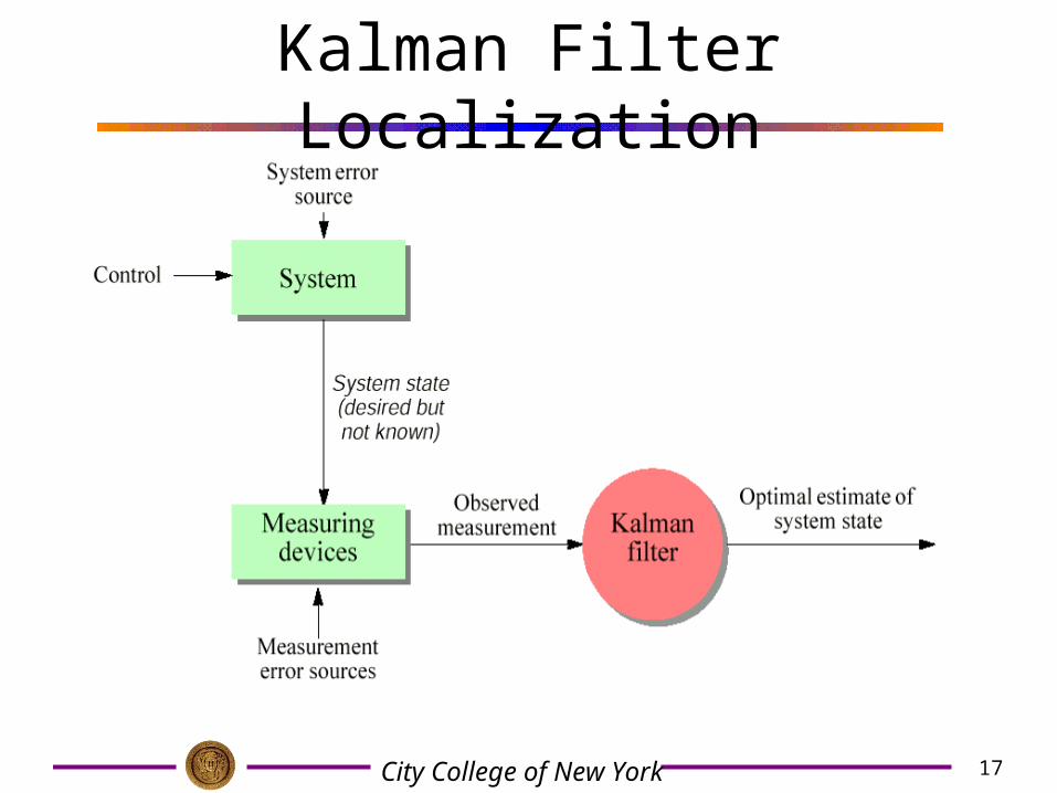
Kalman Filter Localization
18City College of New York
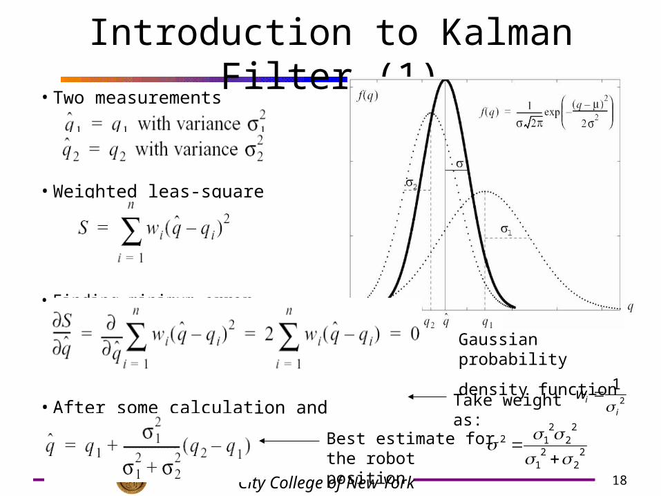
Introduction to Kalman Filter (1)• Two measurements
• Weighted leas-square
• Finding minimum error
• After some calculation and rearrangements
2
1
iiw
Gaussian probability
density function
Take weight as:
Best estimate for the robot position 2
22
1
22
212
2
1
i
iw
19City College of New York
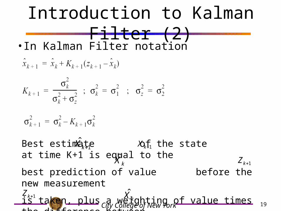
Introduction to Kalman Filter (2)• In Kalman Filter notation
1kXBest estimate of the state at time K+1 is equal to the
best prediction of value before the new measurement
is taken, plus a weighting of value times the difference between
and the best prediction at time k
1ˆ
kX
kX 1kZ
1kZkX
20City College of New York
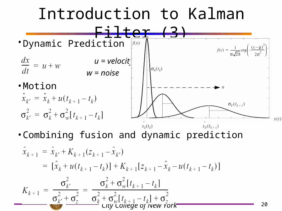
Introduction to Kalman Filter (3)• Dynamic Prediction (robot moving)
u = velocity w = noise
• Motion
• Combining fusion and dynamic prediction
21City College of New York
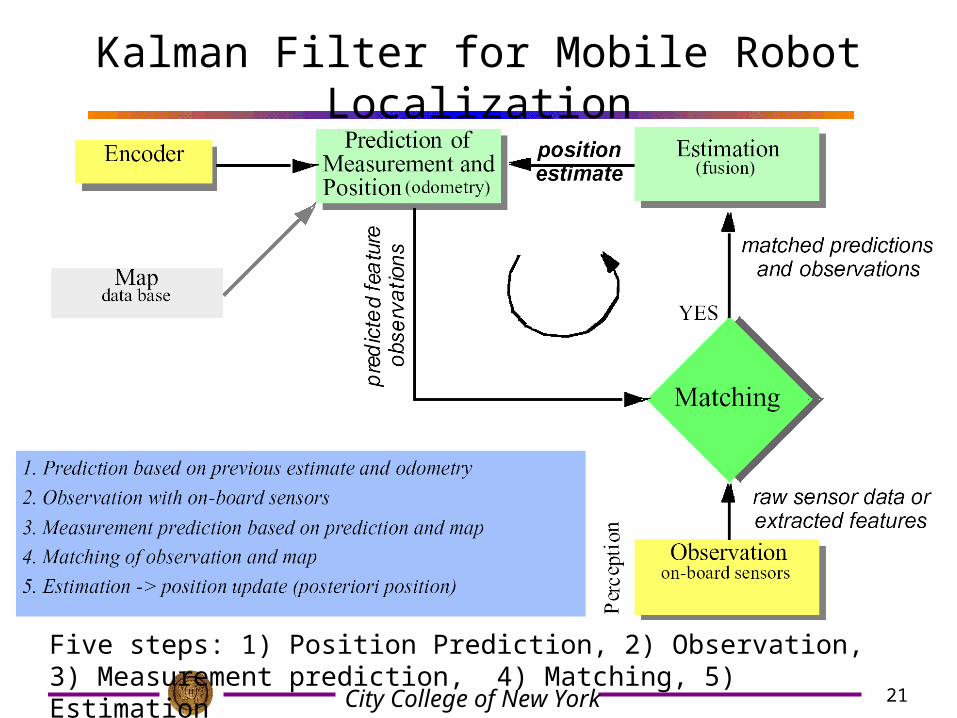
Kalman Filter for Mobile Robot Localization
Five steps: 1) Position Prediction, 2) Observation, 3) Measurement prediction, 4) Matching, 5) Estimation
22City College of New York
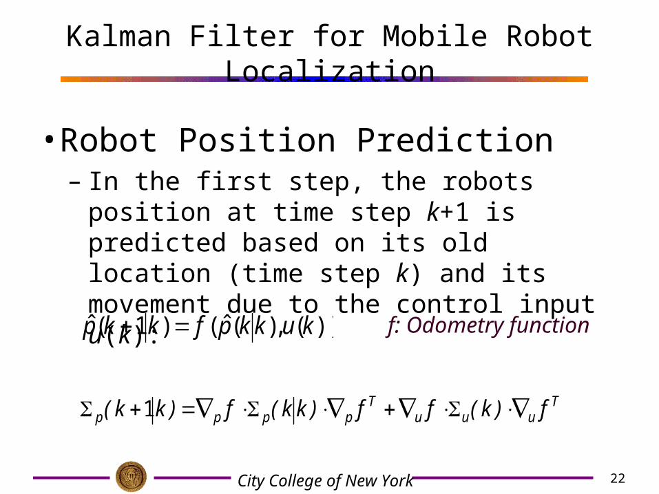
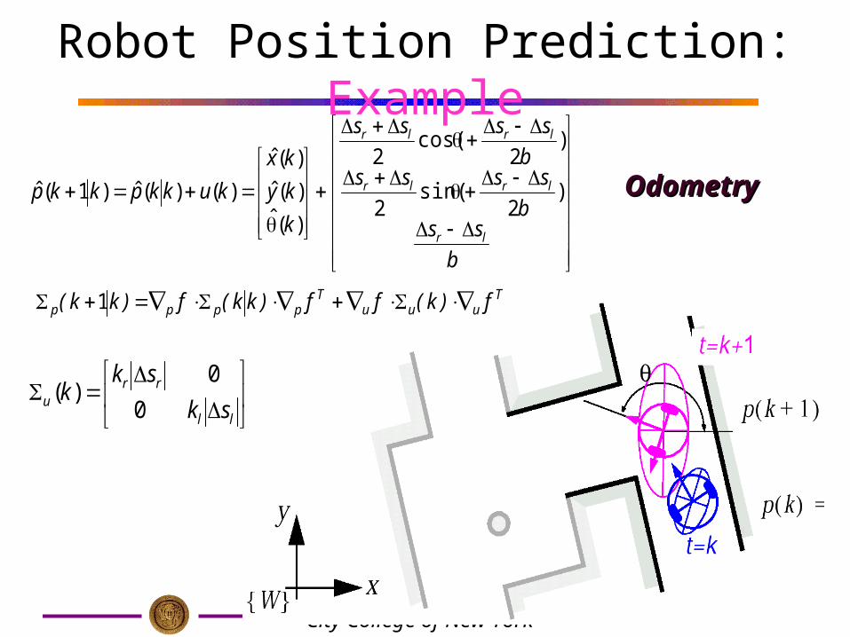
Kalman Filter for Mobile Robot Localization
•Robot Position Prediction– In the first step, the robots position at time
step k+1 is predicted based on its old location (time step k) and its movement due to the control input u(k):
))(,)(ˆ()1(ˆ kukkpfkkp
Tuuu
Tpppp f)k(ff)kk(f)kk( 1
f: Odometry function
23City College of New York
Robot Position Prediction: Example
b
ssb
ssssb
ssss
k
ky
kx
kukkpkkp
lr
lrlr
lrlr
)2
sin(2
)2
cos(2
)(ˆ)(ˆ
)(ˆ
)()(ˆ)1(ˆ
Tuuu
Tpppp f)k(ff)kk(f)kk( 1
ll
rru sk
skk
0
0)(
OdometryOdometry
24City College of New York
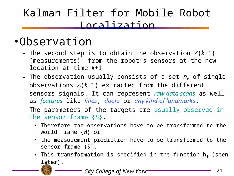
Kalman Filter for Mobile Robot Localization
•Observation– The second step is to obtain the observation Z(k+1) (measurements)
from the robot’s sensors at the new location at time k+1
– The observation usually consists of a set n0 of single observations zj(k+1) extracted from the different sensors signals. It can represent raw data scans as well as features like lines, doors or any kind of landmarks.
– The parameters of the targets are usually observed in the sensor frame {S}.
• Therefore the observations have to be transformed to the world frame {W} or
• the measurement prediction have to be transformed to the sensor frame {S}.
• This transformation is specified in the function hi (seen later).
25City College of New York
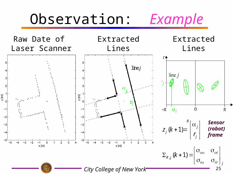
Observation: Example
j
r j
line j
Raw Date of Laser Scanner
Extracted Lines Extracted Lines
in Model Space
jrrr
rjR k
)1(,
j
j
R
j rkz )1(
Sensor (robot) frame
26City College of New York
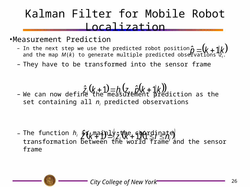
Kalman Filter for Mobile Robot Localization
• Measurement Prediction– In the next step we use the predicted robot position
and the map M(k) to generate multiple predicted observations zt.
– They have to be transformed into the sensor frame
– We can now define the measurement prediction as the set containing all ni predicted observations
– The function hi is mainly the coordinate transformation between the world frame and the sensor frame
kkp 1
kkp,zhkz tii 11
ii nikzkZ 111
27City College of New York
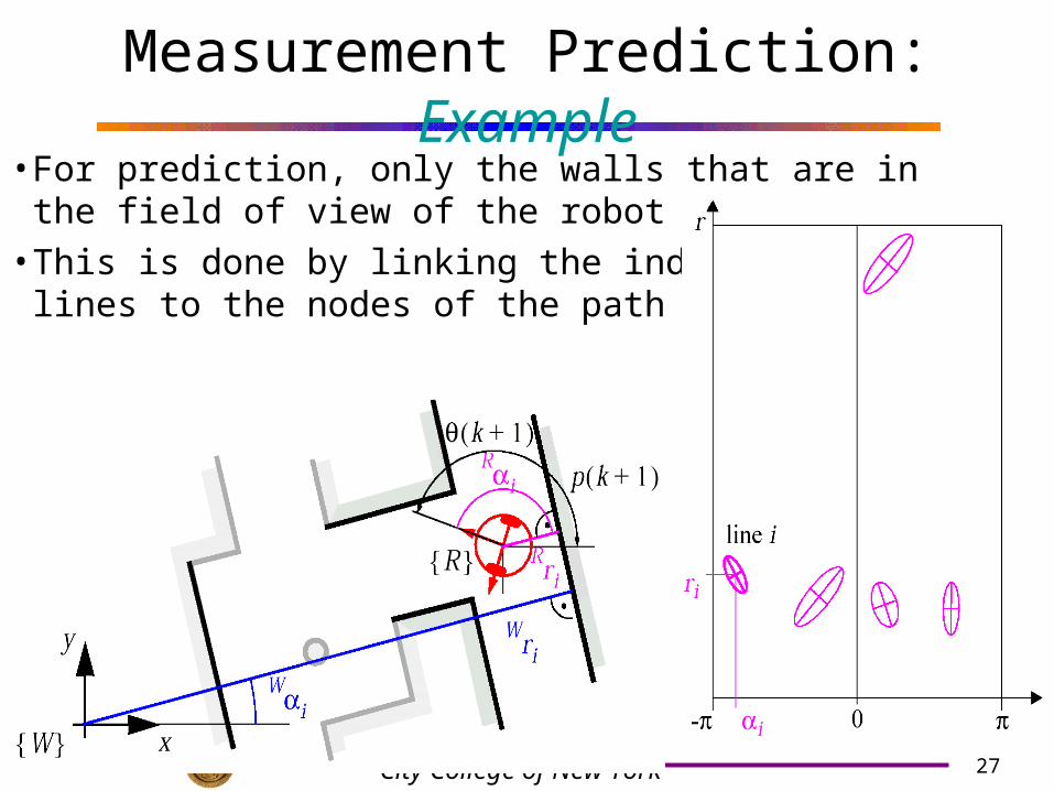
Measurement Prediction: Example• For prediction, only the walls that are in
the field of view of the robot are selected.• This is done by linking the individual
lines to the nodes of the path
28City College of New York
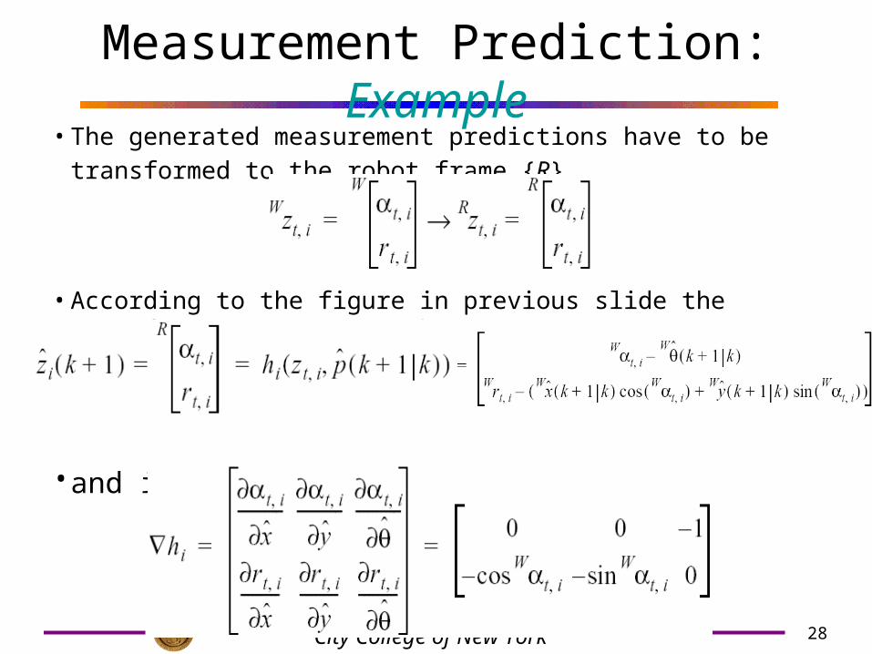
Measurement Prediction: Example• The generated measurement predictions have to be transformed to
the robot frame {R}
• According to the figure in previous slide the transformation is given by
• and its Jacobian by
29City College of New York
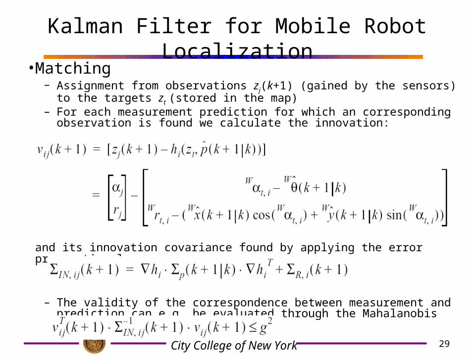
Kalman Filter for Mobile Robot Localization• Matching
– Assignment from observations zj(k+1) (gained by the sensors) to the targets zt (stored in the map)
– For each measurement prediction for which an corresponding observation is found we calculate the innovation:
and its innovation covariance found by applying the error propagation law:
– The validity of the correspondence between measurement and prediction can e.g. be evaluated through the Mahalanobis distance:
30City College of New York
Matching: Example
31City College of New York
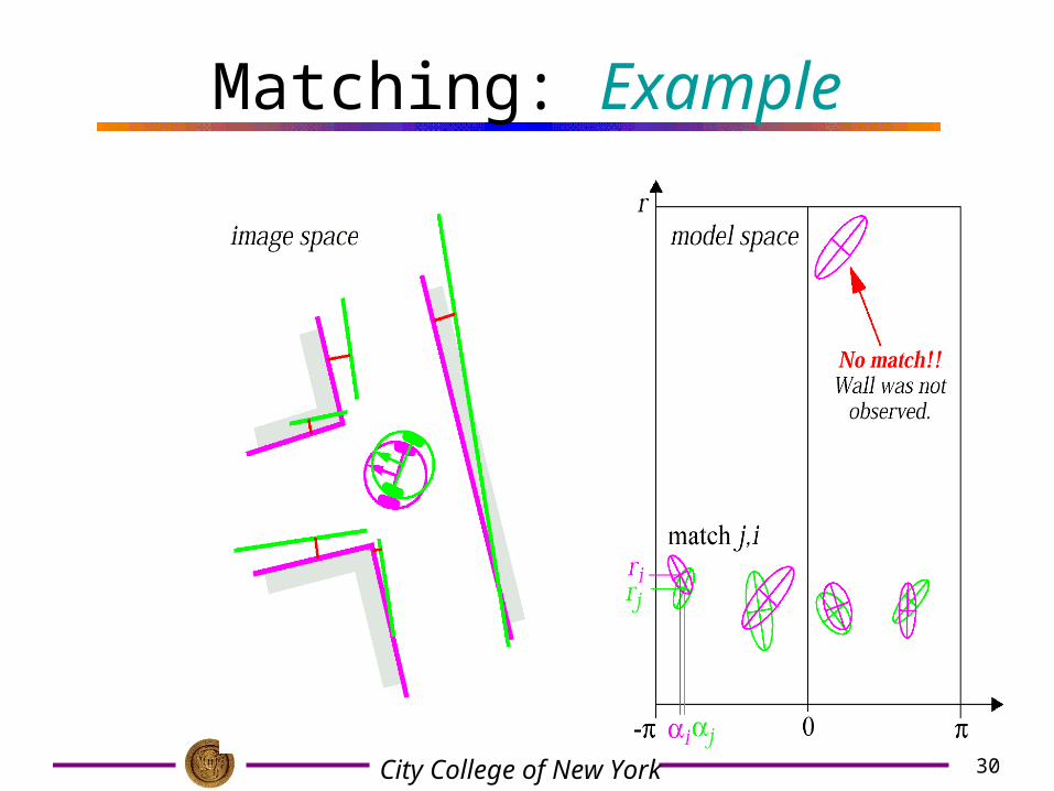
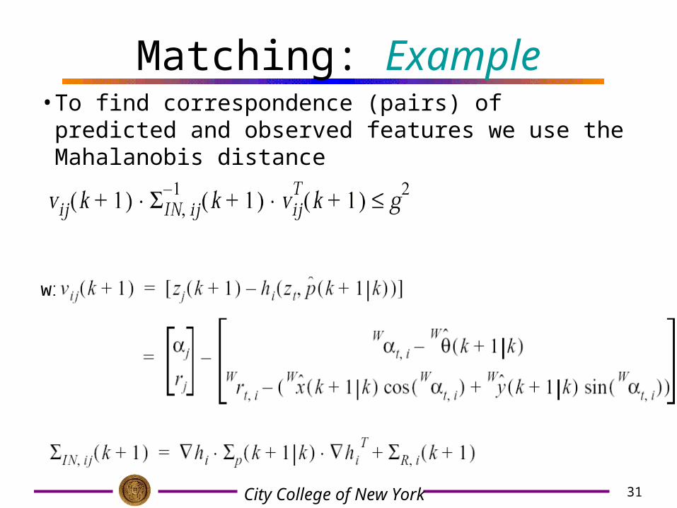
Matching: Example• To find correspondence (pairs) of predicted and observed
features we use the Mahalanobis distance
with
32City College of New York
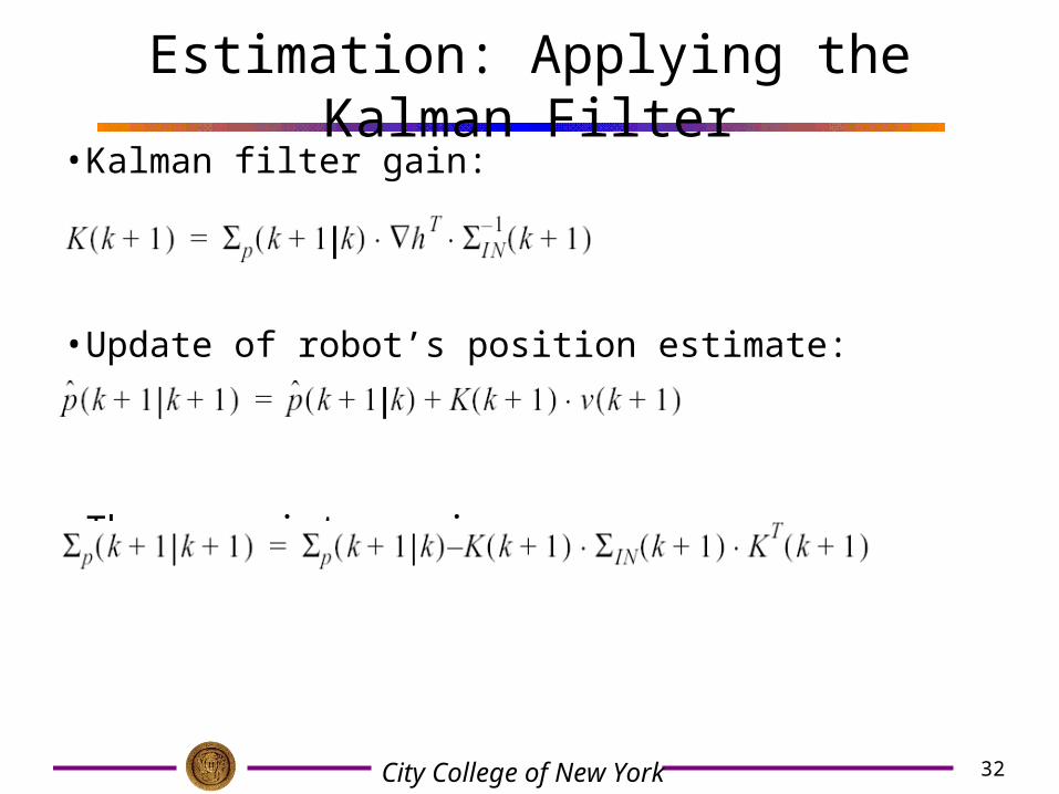
Estimation: Applying the Kalman Filter• Kalman filter gain:
• Update of robot’s position estimate:
• The associate variance
33City College of New York
Estimation: 1D Case
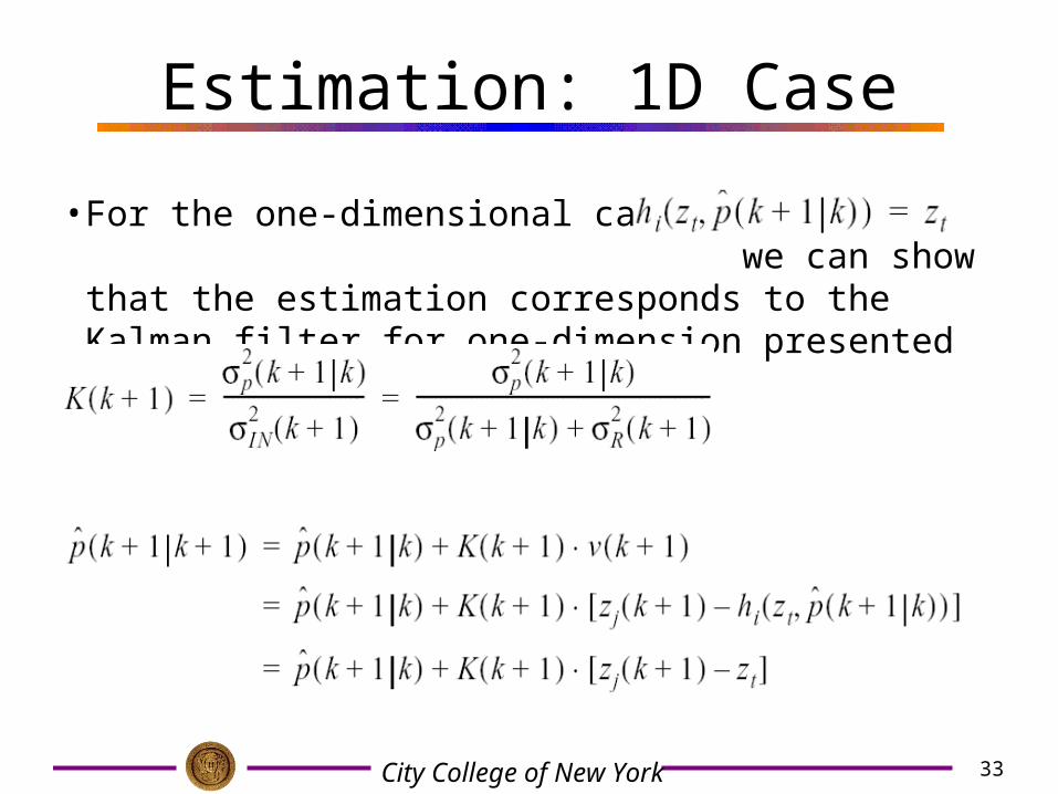
• For the one-dimensional case with we can show that the estimation corresponds to the Kalman filter for one-dimension presented earlier.
34City College of New York
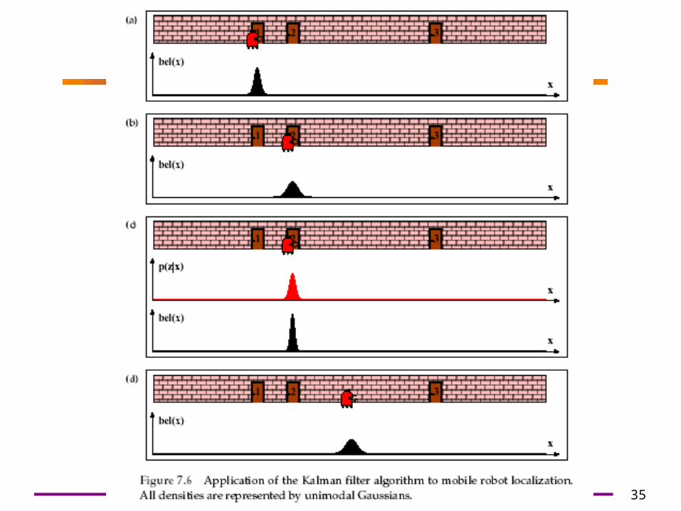
Estimation: Example
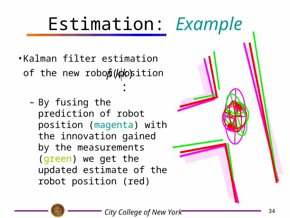
• Kalman filter estimation of the
new robot position : – By fusing the prediction of
robot position (magenta) with the innovation gained by the measurements (green) we get the updated estimate of the robot position (red)
)(ˆ kkp
35City College of New York
36City College of New York
Monte Carlo Localization
• One of the most popular particle filter method for robot localization
• Current Research Topics
• Reference: – Dieter Fox, Wolfram Burgard, Frank Dellaert,
Sebastian Thrun, “Monte Carlo Localization: Efficient Position Estimation for Mobile Robots”, Proc. 16th National Conference on Artificial Intelligence, AAAI’99, July 1999
37City College of New York
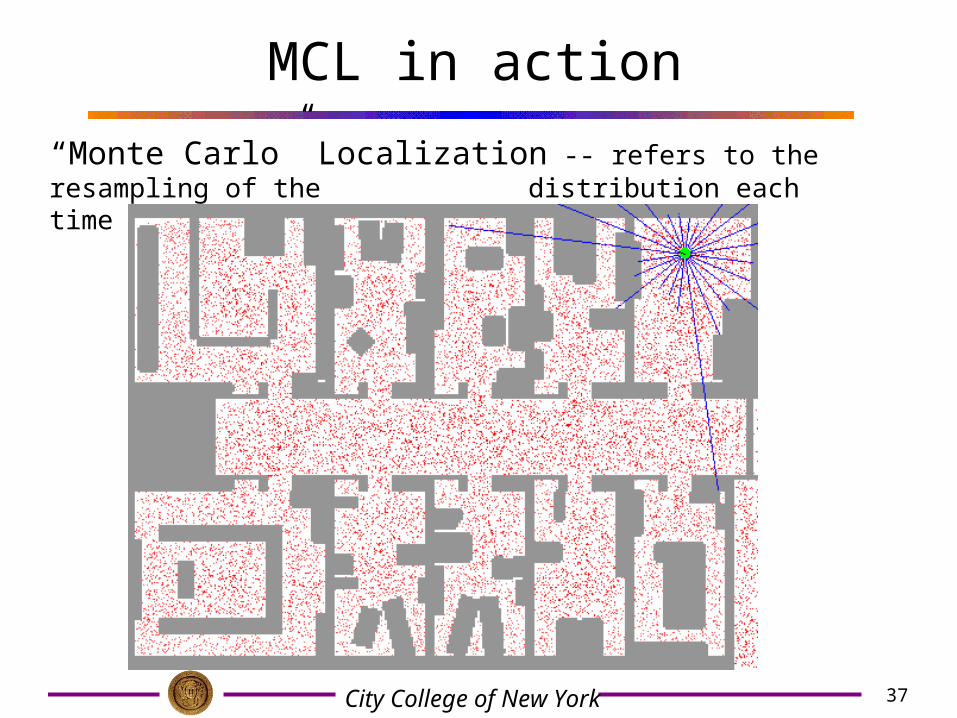
MCL in action
“Monte Carlo” Localization -- refers to the resampling of the distribution each time a new observation is integrated
38City College of New York
Monte Carlo Localization• the probability density function is represented by
samples• randomly drawn from it• it is also able to represent multi-modal distributions,
and thus localize the robot globally• considerably reduces the amount of memory required
and can integrate measurements at a higher rate• state is not discretized and the method is more
accurate than the grid-based methods• easy to implement
39City College of New York
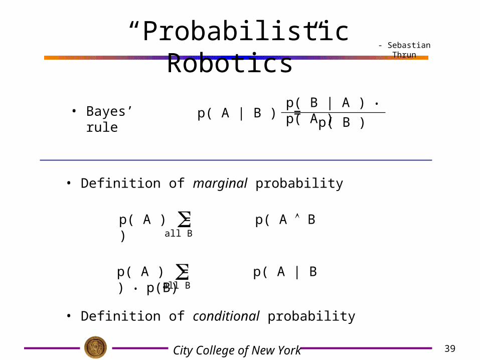
“Probabilistic Robotics”
• Bayes’ rule p( A | B ) = p( B | A ) • p( A )
p( B )
• Definition of marginal probability
p( A ) = p( A | B ) • p(B) all B
p( A ) = p( A B )all B
• Definition of conditional probability
- Sebastian Thrun
40City College of New York
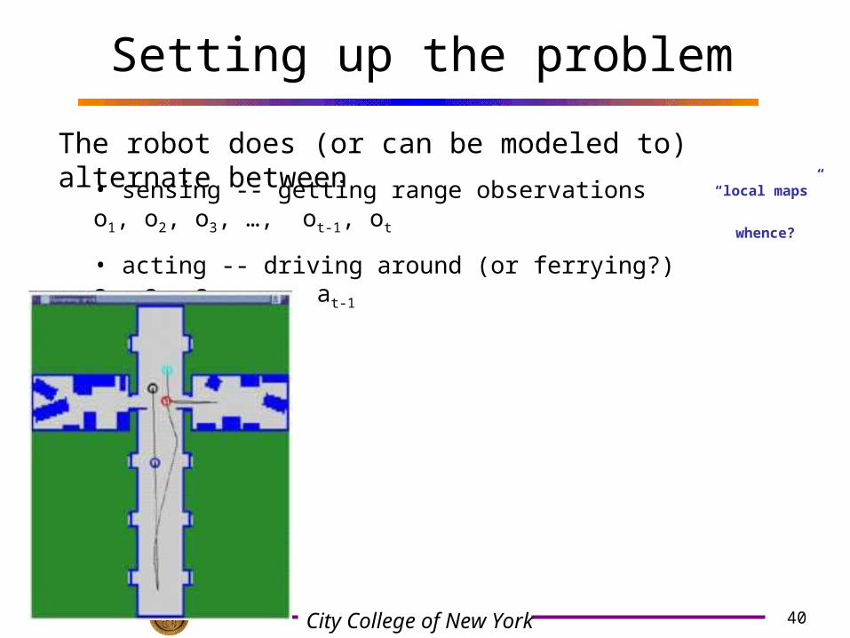
Setting up the problem
The robot does (or can be modeled to) alternate between
• sensing -- getting range observations o1, o2, o3, …, ot-1, ot
• acting -- driving around (or ferrying?) a1, a2, a3, …, at-1
“local maps”
whence?
41City College of New York
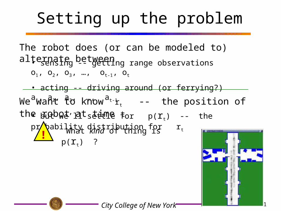
Setting up the problem
The robot does (or can be modeled to) alternate between
• sensing -- getting range observations o1, o2, o3, …, ot-1, ot
• acting -- driving around (or ferrying?) a1, a2, a3, …, at-1
We want to know rt -- the position of the robot at time t
• but we’ll settle for p(rt) -- the probability distribution for rt
! What kind of thing is p(rt) ?
42City College of New York
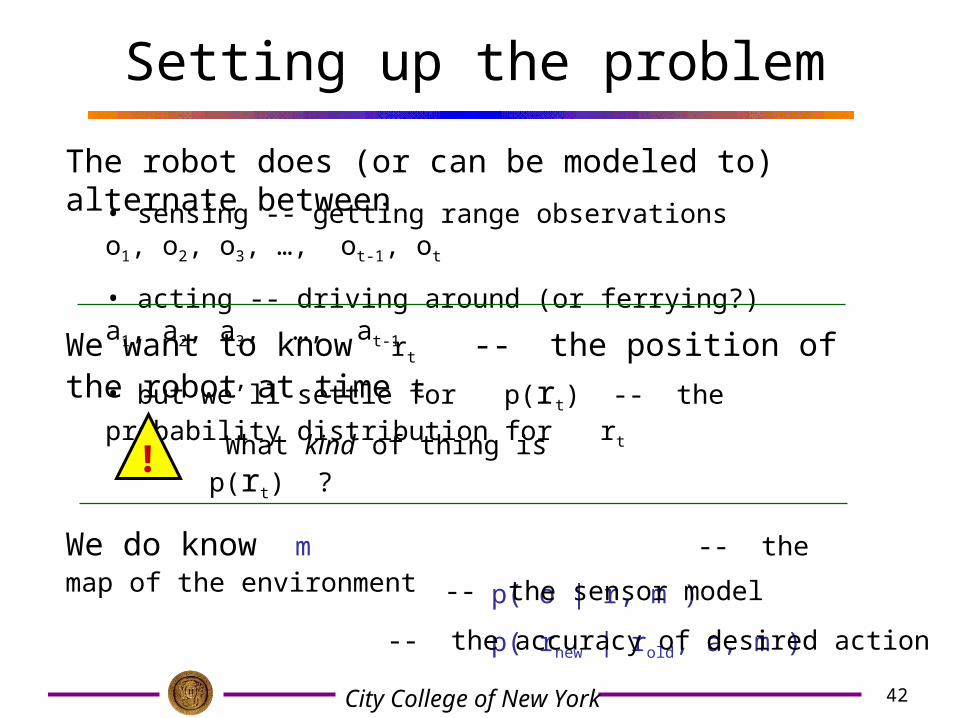
Setting up the problem
The robot does (or can be modeled to) alternate between
• sensing -- getting range observations o1, o2, o3, …, ot-1, ot
• acting -- driving around (or ferrying?) a1, a2, a3, …, at-1
We want to know rt -- the position of the robot at time t
We do know m -- the map of the environment
• but we’ll settle for p(rt) -- the probability distribution for rt
! What kind of thing is p(rt) ?
p( o | r, m )
p( rnew | rold, a, m )
-- the sensor model
-- the accuracy of desired action a
43City College of New York
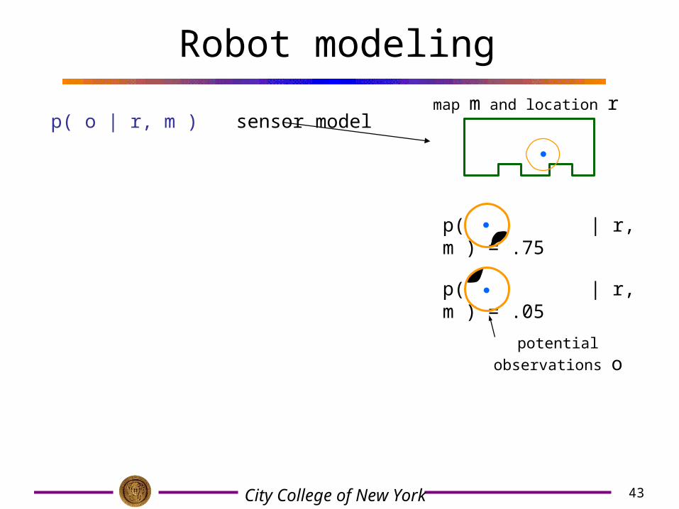
Robot modeling
p( o | r, m ) sensor modelmap m and location r
p( | r, m ) = .75
p( | r, m ) = .05
potential observations o
44City College of New York
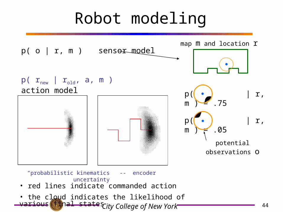
Robot modeling
p( o | r, m ) sensor model
p( rnew | rold, a, m ) action model
“probabilistic kinematics” -- encoder uncertainty
• red lines indicate commanded action
• the cloud indicates the likelihood of various final states
map m and location r
p( | r, m ) = .75
p( | r, m ) = .05
potential observations o
45City College of New York
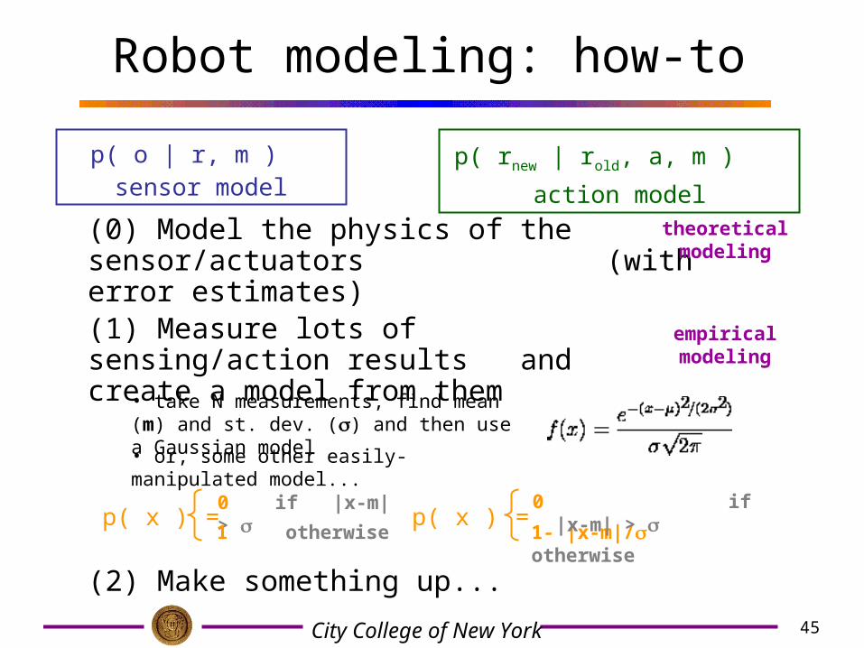
Robot modeling: how-to
p( o | r, m ) sensor model
p( rnew | rold, a, m ) action
model
(0) Model the physics of the sensor/actuators(with error estimates)
(1) Measure lots of sensing/action resultsand create a model from them
theoretical modeling
empirical modeling
• take N measurements, find mean (m) and st. dev. () and then use a Gaussian model
• or, some other easily-manipulated model...
(2) Make something up...
p( x ) = p( x ) = 0 if |x-m| >
1 otherwise 1- |x-m|/ otherwise
0 if |x-m| >
46City College of New York
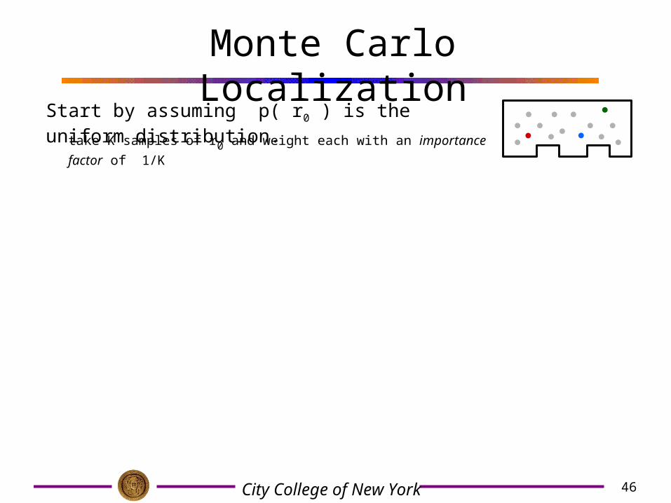
Monte Carlo Localization
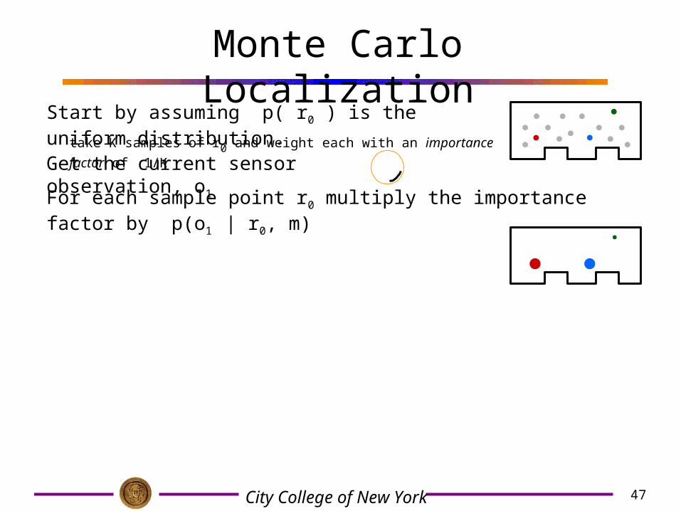
Start by assuming p( r0 ) is the uniform distribution.
take K samples of r0 and weight each with an importance factor
of 1/K
47City College of New York
Monte Carlo Localization
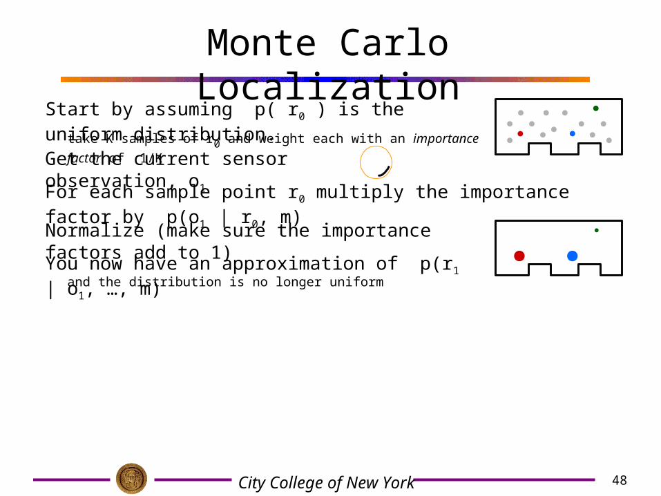
Start by assuming p( r0 ) is the uniform distribution.
Get the current sensor observation, o1
For each sample point r0 multiply the importance factor by p(o1 | r0, m)
take K samples of r0 and weight each with an importance factor
of 1/K
48City College of New York
Monte Carlo Localization
Start by assuming p( r0 ) is the uniform distribution.
Get the current sensor observation, o1
For each sample point r0 multiply the importance factor by p(o1 | r0, m)
take K samples of r0 and weight each with an importance factor
of 1/K
Normalize (make sure the importance factors add to 1)
You now have an approximation of p(r1 | o1, …, m) and the distribution is no longer uniform

49City College of New York
Monte Carlo Localization
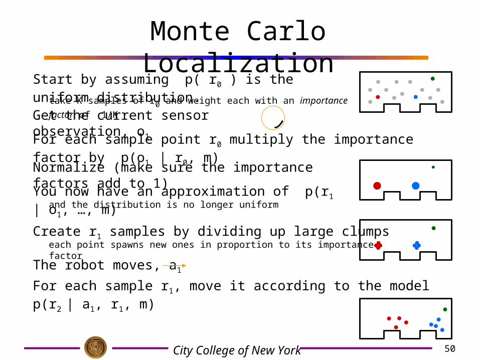
Start by assuming p( r0 ) is the uniform distribution.
Get the current sensor observation, o1
For each sample point r0 multiply the importance factor by p(o1 | r0, m)
take K samples of r0 and weight each with an importance factor
of 1/K
Normalize (make sure the importance factors add to 1)
You now have an approximation of p(r1 | o1, …, m)
Create r1 samples by dividing up large clumps
and the distribution is no longer uniform
each point spawns new ones in proportion to its importance factor
50City College of New York
Monte Carlo Localization
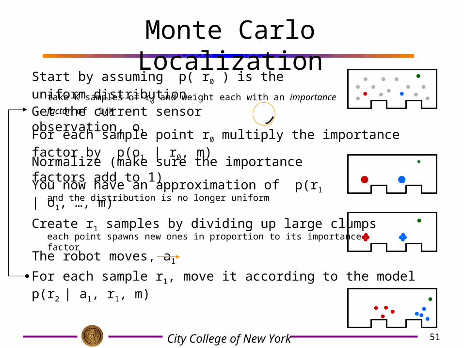
Start by assuming p( r0 ) is the uniform distribution.
Get the current sensor observation, o1
For each sample point r0 multiply the importance factor by p(o1 | r0, m)
take K samples of r0 and weight each with an importance factor
of 1/K
Normalize (make sure the importance factors add to 1)
You now have an approximation of p(r1 | o1, …, m)
Create r1 samples by dividing up large clumps
and the distribution is no longer uniform
The robot moves, a1
each point spawns new ones in proportion to its importance factor
For each sample r1, move it according to the model p(r2 | a1, r1, m)
51City College of New York
Monte Carlo Localization
Start by assuming p( r0 ) is the uniform distribution.
Get the current sensor observation, o1
For each sample point r0 multiply the importance factor by p(o1 | r0, m)
take K samples of r0 and weight each with an importance factor
of 1/K
Normalize (make sure the importance factors add to 1)
You now have an approximation of p(r1 | o1, …, m)
Create r1 samples by dividing up large clumps
and the distribution is no longer uniform
The robot moves, a1
each point spawns new ones in proportion to its importance factor
For each sample r1, move it according to the model p(r2 | a1, r1, m)

52City College of New York
MCL in action
“Monte Carlo” Localization -- refers to the resampling of the distribution each time a new observation is integrated
53City College of New York
Discussion: MCL
54City College of New York
References
1. Dieter Fox, Wolfram Burgard, Frank Dellaert, Sebastian Thrun, “Monte Carlo Localization: Efficient Position Estimation for Mobile Robots”, Proc. 16th National Conference on Artificial Intelligence, AAAI’99, July 1999
2. Dieter Fox, Wolfram Burgard, Sebastian Thrun, “Markov Localization for Mobile Robots in Dynamic Environments”, J. of Artificial Intelligence Research 11 (1999) 391-427
3. Sebastian Thrun, “Probabilistic Algorithms in Robotics”, Technical Report CMU-CS-00-126, School of Computer Science, Carnegie Mellon University, Pittsburgh, USA, 2000