civil formulas - gtucampus engineeringgaurav... · design of a solid-bowl centrifuge for sludge...
TRANSCRIPT


CIVILENGINEERING
FORMULAS

ABOUT THE AUTHOR
Tyler G. Hicks, P.E., is a consulting engineer and a successful engi-neering book author. He has worked in plant design and operationin a variety of industries, taught at several engineering schools, andlectured both in the United States and abroad. Mr. Hicks holds abachelor’s degree in Mechanical Engineering from Cooper UnionSchool of Engineering in New York. He is the author of more than100 books in engineering and related fields.

CIVILENGINEERING
FORMULAS
Tyler G. Hicks, P.E.
International Engineering AssociatesMember: American Society of Mechanical Engineers
United States Naval Institute
Second Edition
New York Chicago San Francisco Lisbon London Madrid
Mexico City Milan New Delhi San Juan Seoul
Singapore Sydney Toronto

Copyright © 2010, 2002 by The McGraw-Hill Companies, Inc. All rights reserved. Except as permittedunder the United States Copyright Act of 1976, no part of this publication may be reproduced or distrib-uted in any form or by any means, or stored in a database or retrieval system, without the prior writtenpermission of the publisher.
ISBN: 978-0-07-161470-2
MHID: 0-07-161470-2
The material in this eBook also appears in the print version of this title: ISBN: 978-0-07-161469-6,MHID: 0-07-161469-9.
All trademarks are trademarks of their respective owners. Rather than put a trademark symbol after everyoccurrence of a trademarked name, we use names in an editorial fashion only, and to the benefit of thetrademark owner, with no intention of infringement of the trademark. Where such designations appearin this book, they have been printed with initial caps.
McGraw-Hill eBooks are available at special quantity discounts to use as premiums and sales promotions, or for use in corporate training programs. To contact a representative please e-mail us [email protected].
Information contained in this work has been obtained by The McGraw-Hill Companies, Inc. (“McGraw-Hill”) from sources believed to be reliable. However, neither McGraw-Hill nor its authors guarantee theaccuracy or completeness of any information published herein, and neither McGraw-Hill nor its authorsshall be responsible for any errors, omissions, or damages arising out of use of this information. Thiswork is published with the understanding that McGraw-Hill and its authors are supplying informationbut are not attempting to render engineering or other professional services. If such services are required,the assistance of an appropriate professional should be sought.
TERMS OF USE
This is a copyrighted work and The McGraw-Hill Companies, Inc. (“McGraw-Hill”) and its licensorsreserve all rights in and to the work. Use of this work is subject to these terms. Except as permitted underthe Copyright Act of 1976 and the right to store and retrieve one copy of the work, you may not decompile, disassemble, reverse engineer, reproduce, modify, create derivative works based upon, transmit, distribute, disseminate, sell, publish or sublicense the work or any part of it without McGraw-Hill’s prior consent. You may use the work for your own noncommercial and personal use; anyother use of the work is strictly prohibited. Your right to use the work may be terminated if you fail tocomply with these terms.
THE WORK IS PROVIDED “AS IS.” McGRAW-HILL AND ITS LICENSORS MAKE NO GUARAN-TEES OR WARRANTIES AS TO THE ACCURACY, ADEQUACY OR COMPLETENESS OF ORRESULTS TO BE OBTAINED FROM USING THE WORK, INCLUDING ANY INFORMATIONTHAT CAN BE ACCESSED THROUGH THE WORK VIA HYPERLINK OR OTHERWISE, ANDEXPRESSLY DISCLAIM ANY WARRANTY, EXPRESS OR IMPLIED, INCLUDING BUT NOTLIMITED TO IMPLIED WARRANTIES OF MERCHANTABILITY OR FITNESS FOR A PARTICU-LAR PURPOSE. McGraw-Hill and its licensors do not warrant or guarantee that the functions containedin the work will meet your requirements or that its operation will be uninterrupted or error free. NeitherMcGraw-Hill nor its licensors shall be liable to you or anyone else for any inaccuracy, error or omission,regardless of cause, in the work or for any damages resulting therefrom. McGraw-Hill has no responsibility for the content of any information accessed through the work. Under no circumstancesshall McGraw-Hill and/or its licensors be liable for any indirect, incidental, special, punitive, consequen-tial or similar damages that result from the use of or inability to use the work, even if any of them hasbeen advised of the possibility of such damages. This limitation of liability shall apply to any claim orcause whatsoever whether such claim or cause arises in contract, tort or otherwise.

CONTENTS
Preface xi
Acknowledgments xiii
How to Use This Book xv
Chapter 1. Conversion Factors for Civil Engineering Practice 1
Chapter 2. Beam Formulas 11
Continuous Beams / 11Ultimate Strength of Continuous Beams / 46Beams of Uniform Strength / 52Safe Loads for Beams of Various Types / 53Rolling and Moving Loads / 53Curved Beams / 65Elastic Lateral Buckling of Beams / 69Combined Axial and Bending Loads / 72Unsymmetrical Bending / 73Eccentric Loading / 73Natural Circular Frequencies and Natural Periods of Vibration of Prismatic Beams / 74
Torsion in Structural Members / 76Strain Energy in Structural Members / 76Fixed-End Moments in Beams / 79
Chapter 3. Column Formulas 81
General Considerations / 81Short Columns / 81Eccentric Loads on Columns / 83Columns of Special Materials / 88Column Base Plate Design / 90American Institute of Steel Construction Allowable-Stress Design Approach / 91
Composite Columns / 92Elastic Flexural Buckling of Columns / 94Allowable Design Loads for Aluminum Columns / 96Ultimate Strength Design Concrete Columns / 97Design of Axially Loaded Steel Columns / 102
v

Chapter 4. Piles and Piling Formulas 105
Allowable Loads on Piles / 105Laterally Loaded Vertical Piles / 105Toe Capacity Load / 107Groups of Piles / 107Foundation-Stability Analysis / 109Axial-Load Capacity of Single Piles / 112Shaft Settlement / 112Shaft Resistance in Cohesionless Soils / 113
Chapter 5. Concrete formulas 115
Reinforced Concrete / 115Water/Cementitious Materials Ratio / 115Job Mix Concrete Volume / 116Modulus of Elasticity of Concrete / 116Tensile Strength of Concrete / 117Reinforcing Steel / 117Continuous Beams and One-Way Slabs / 117Design Methods for Beams, Columns, and Other Members / 118
Properties in the Hardened State / 127Tension Development Lengths / 128Compression Development Lengths / 128Crack Control of Flexural Members / 128Required Strength / 129Deflection Computations and Criteria for Concrete Beams / 130
Ultimate-Strength Design of Rectangular Beams with Tension Reinforcement Only / 130
Working-Stress Design of Rectangular Beams with Tension Reinforcement Only / 133
Ultimate-Strength Design of Rectangular Beams with Compression Bars / 135
Working-Stress Design of Rectangular Beams with Compression Bars / 136
Ultimate-Strength Design of I- and T-beams / 138Working-Stress Design of I- and T-beams / 138Ultimate-Strength Design for Torsion / 140Working-Stress Design for Torsion / 141Flat-Slab Construction / 142Flat-Plate Construction / 142Shear in Slabs / 145Column Moments / 146Spirals / 147Braced and Unbraced Frames / 147Shear Walls / 148Concrete Gravity Retaining Walls / 150Cantilever Retaining Walls / 153Wall Footings / 155
vi CONTENTS

Chapter 6. Timber Engineering Formulas 157
Grading of Lumber / 157Size of Lumber / 157Bearing / 159Beams / 159Columns / 160Combined Bending and Axial Load / 161Compression at Angle to Grain / 161Recommendations of the Forest Products Laboratory / 162Compression on Oblique Plane / 163Adjustment Factors for Design Values / 164Fasteners for Wood / 169Adjustment of Design Values for Connections with Fasteners / 171
Roof Slope to Prevent Ponding / 172Bending and Axial Tension / 173Bending and Axial Compression / 173Solid Rectangular or Square Columns with Flat Ends / 174
Chapter 7. Surveying Formulas 177
Units of Measurement / 177Theory of Errors / 178Measurement of Distance with Tapes / 179Vertical Control / 182Stadia Surveying / 183Photogrammetry / 184
Chapter 8. Soil and Earthwork Formulas 185
Physical Properties of Soils / 185Index Parameters for Soils / 186Relationship of Weights and Volumes in Soils / 186Internal Friction and Cohesion / 188Vertical Pressures in Soils / 188Lateral Pressures in Soils, Forces on Retaining Walls / 189
Lateral Pressure of Cohesionless Soils / 190Lateral Pressure of Cohesive Soils / 191Water Pressure / 191Lateral Pressure from Surcharge / 191Stability of Slopes / 192Bearing Capacity of Soils / 192Settlement under Foundations / 193Soil Compaction Tests / 193Compaction Equipment / 195Formulas for Earthmoving / 196Scraper Production / 197Vibration Control in Blasting / 198
CONTENTS vii

Chapter 9. Building and Structures Formulas 207
Load-and-Resistance Factor Design for Shear in Buildings / 207
Allowable-Stress Design for Building Columns / 208Load-and-Resistance Factor Design for Building Columns / 209Allowable-Stress Design for Building Beams / 209Load-and-Resistance Factor Design for Building Beams / 211Allowable-Stress Design for Shear in Buildings / 214Stresses in Thin Shells / 215Bearing Plates / 216Column Base Plates / 217Bearing on Milled Surfaces / 218Plate Girders in Buildings / 219Load Distribution to Bents and Shear Walls / 220Combined Axial Compression or Tension and Bending / 221Webs under Concentrated Loads / 222Design of Stiffeners under Loads / 224Fasteners in Buildings / 225Composite Construction / 225Number of Connectors Required for Building Construction / 226
Ponding Considerations in Buildings / 228Lightweight Steel Construction / 228Choosing the Most Economic Structural Steel / 239Steel Carbon Content and Weldability / 240Statically Indeterminate Forces and Moments in Building Structures / 241
Roof Live Loads / 244
Chapter 10. Bridge and Suspension-Cable Formulas 249
Shear Strength Design for Bridges / 249Allowable-Stress Design for Bridge Columns / 250Load-and-Resistance Factor Design for Bridge Columns / 250Additional Bridge Column Formulas / 251Allowable-Stress Design for Bridge Beams / 254Stiffeners on Bridge Girders / 255Hybrid Bridge Girders / 256Load-Factor Design for Bridge Beams / 256Bearing on Milled Surfaces / 258Bridge Fasteners / 258Composite Construction in Highway Bridges / 259Number of Connectors in Bridges / 261Allowable-Stress Design for Shear in Bridges / 262Maximum Width/Thickness Ratios for Compression Elements for Highway Bridges / 263Suspension Cables / 263General Relations for Suspension Cables / 267Cable Systems / 272Rainwater Accumulation and Drainage on Bridges / 273
viii CONTENTS

Chapter 11. Highway and Road Formulas 275
Circular Curves / 275Parabolic Curves / 277Highway Curves and Driver Safety / 278Highway Alignments / 279Structural Numbers for Flexible Pavements / 281Transition (Spiral) Curves / 284Designing Highway Culverts / 285American Iron and Steel Institute (AISI) Design Procedure / 286
Chapter 12. Hydraulics and Waterworks Formulas 291
Capillary Action / 291Viscosity / 291Pressure on Submerged Curved Surfaces / 295Fundamentals of Fluid Flow / 296Similitude for Physical Models / 298Fluid Flow in Pipes / 300Pressure (Head) Changes Caused by Pipe Size Change / 306
Flow through Orifices / 308Fluid Jets / 310Orifice Discharge into Diverging Conical Tubes / 311Water Hammer / 312Pipe Stresses Perpendicular to the Longitudinal Axis / 312
Temperature Expansion of Pipe / 313Forces due to Pipe Bends / 313Culverts / 315Open-Channel Flow / 318Manning’s Equation for Open Channels / 320Hydraulic Jump / 321Nonuniform Flow in Open Channels / 323Weirs / 329Flow over Weirs / 330Prediction of Sediment-Delivery Rate / 332Evaporation and Transpiration / 332Method for Determining Runoff for Minor Hydraulic Structures / 333
Computing Rainfall Intensity / 333Groundwater / 334Water Flow for Fire Fighting / 335Flow from Wells / 335Economical Sizing of Distribution Piping / 336Venturi Meter Flow Computation / 336Hydroelectric Power Generation / 337Pumps and Pumping Systems / 338Hydraulic Turbines / 344Dams / 348
CONTENTS ix

Chapter 13. Stormwater, Sewage, Sanitary Wastewater, and Environmental Protection 361
Determining Storm Water Flow / 361Flow Velocity in Straight Sewers / 361Design of a Complete-Mix Activated Sludge Reactor / 364Design of a Circular Settling Tank / 368Sizing a Polymer Dilution/Feed System / 369Design of a Solid-Bowl Centrifuge for Sludge Dewatering / 369Design of a Trickling Filter Using the NRC Equations / 371Design of a Rapid-Mix Basin and Flocculation Basin / 373Design of an Aerobic Digester / 374Design of a Plastic Media Trickling Filter / 375Design of an Anaerobic Digestor / 377Design of a Chlorination System for Wastewater Disinfection / 379Sanitary Sewer System Design / 380Design of an Aerated Grit Chamber / 383
Index 385
x CONTENTS

PREFACE
The second edition of this handy book presents some 2,500 formulas and calcu-lation guides for civil engineers to help them in the design office, in the field,and on a variety of construction jobs, anywhere in the world. These formulasand guides are also useful to design drafters, structural engineers, bridge engi-neers, foundation builders, field engineers, professional-engineer license exam-ination candidates, concrete specialists, timber-structure builders, and studentsin a variety of civil engineering pursuits.
The book presents formulas needed in 13 different specialized branches ofcivil engineering—beams and girders, columns, piles and piling, concretestructures, timber engineering, surveying, soils and earthwork, building struc-tures, bridges, suspension cables, highways and roads, hydraulics and openchannel flow, stormwater, sewage, sanitary wastewater, and environmentalprotection. Some 500 formulas and guides have been added to this second edi-tion of the book.
Key formulas are presented for each of the major topics listed above.Each formula is explained so the engineer, drafter, or designer knows how,where, and when to use the formula in professional work. Formula units aregiven in both the United States Customary System (USCS) and SystemInternational (SI). Hence, the content of this book is usable throughout theworld. To assist the civil engineer using these formulas in worldwide engineer-ing practice, a comprehensive tabulation of conversion factors is presentedin Chap. 1.
New content is this second edition spans the world of civil engineering.Specific new topics include columns for supporting commercial wind turbinesused in onshore and offshore renewable energy projects, design of axiallyloaded steel columns, strain energy in structural members, shaft twist formulas,new retaining wall formulas and data, solid-wood rectangular column design,blasting operations for earth and rock removal or relocation, hydraulic turbinesfor power generation, dams of several types (arch, buttress, earth), comparisonsof key hydraulic formulas (Darcy, Manning, Hazen-Williams), and a completenew chapter on stormwater, sewage, sanitary wastewater, and environmentalprotection.
In assembling this collection of formulas, the author was guided by expertswho recommended the areas of greatest need for a handy book of practical andapplied civil engineering formulas.
Sources for the formulas presented here include the various regulatory andindustry groups in the field of civil engineering, authors of recognized books onimportant topics in the field, drafters, researchers in the field of civil engineer-ing, and a number of design engineers who work daily in the field of civil engi-neering. These sources are cited in the Acknowledgments.
xi

When using any of the formulas in this book that may come from an indus-try or regulatory code, the user is cautioned to consult the latest version of thecode. Formulas may be changed from one edition of code to the next. In a workof this magnitude it is difficult to include the latest formulas from the numerousconstantly changing codes. Hence, the formulas given here are those current atthe time of publication of this book.
In a work this large it is possible that errors may occur. Hence, the authorwill be grateful to any user of the book who detects an error and calls it to theauthor’s attention. Just write the author in care of the publisher. The error willbe corrected in the next printing.
In addition, if a user believes that one or more important formulas have beenleft out, the author will be happy to consider them for inclusion in the next editionof the book. Again, just write to him in care of the publisher.
Tyler G. Hicks, P.E.
xii PREFACE

ACKNOWLEDGMENTS
Many engineers, professional societies, industry associations, and governmen-tal agencies helped the author find and assemble the thousands of formulas pre-sented in this book. Hence, the author wishes to acknowledge this help andassistance.
The author’s principal helper, advisor, and contributor was late Frederick S. Merritt, P.E., Consulting Engineer. For many years Fred and the author wereeditors on companion magazines at The McGraw-Hill Companies. Fred was aneditor on Engineering-News Record, whereas the author was an editor onPower magazine. Both lived on Long Island and traveled on the same railroadto and from New York City, spending many hours together discussing engi-neering, publishing, and book authorship.
When the author was approached by the publisher to prepare this book, heturned to Fred Merritt for advice and help. Fred delivered, preparing many ofthe formulas in this book and giving the author access to many more in Fred’sextensive files and published materials. The author is most grateful to Fred forhis extensive help, advice, and guidance.
Other engineers and experts to whom the author is indebted for formulasincluded in this book are Roger L. Brockenbrough, Calvin Victor Davis, F. E.Fahey, Gary B. Hemphill, P.E., Metcalf & Eddy, Inc., George Tchobanoglous,Demetrious E. Tonias, P.E., and Kevin D. Wills, P.E.
Further, the author thanks many engineering societies, industry associations,and governmental agencies whose work is referred to in this publication. Theseorganizations provide the framework for safe design of numerous structures ofmany different types.
The author also thanks Larry Hager, Senior Editor, Professional Group, TheMcGraw-Hill Companies, for his excellent guidance and patience during thelong preparation of the manuscript for this book. Finally, the author thanks hiswife, Mary Shanley Hicks, a publishing professional, who always most willinglyoffered help and advice when needed.
Specific publications consulted during the preparation of this text includeAmerican Association of State Highway and Transportation Officials(AASHTO) “Standard Specifications for Highway Bridges”; American Con-crete Institute (ACI) “Building Code Requirements for Reinforced Concrete”;American Institute of Steel Construction (AISC) “Manual of Steel Construc-tion,” “Code of Standard Practice,” and “Load and Resistance Factor DesignSpecifications for Structural Steel Buildings”; American Railway Engineer-ing Association (AREA) “Manual for Railway Engineering”; American Societyof Civil Engineers (ASCE) “Ground Water Management”; and AmericanWater Works Association (AWWA) “Water Quality and Treatment.” In addition,
xiii

the author consulted several hundred civil engineering reference and textbooksdealing with the topics in the current book. The author is grateful to the writersof all the publications cited here for the insight they gave him to civil engi-neering formulas. A number of these works are also cited in the text of thisbook.
xiv ACKNOWLEDGMENTS

HOW TO USE THIS BOOK
The formulas presented in this book are intended for use by civil engineersin every aspect of their professional work—design, evaluation, construction,repair, etc.
To find a suitable formula for the situation you face, start by consulting theindex. Every effort has been made to present a comprehensive listing of all for-mulas in the book.
Once you find the formula you seek, read any accompanying text giving back-ground information about the formula. Then when you understand the formulaand its applications, insert the numerical values for the variables in the formula.Solve the formula and use the results for the task at hand.
Where a formula may come from a regulatory code, or where a code existsfor the particular work being done, be certain to check the latest edition of theapplicable code to see that the given formula agrees with the code formula. If itdoes not agree, be certain to use the latest code formula available. Remember,as a design engineer you are responsible for the structures you plan, design, andbuild. Using the latest edition of any governing code is the only sensible way toproduce a safe and dependable design that you will be proud to be associatedwith. Further, you will sleep more peacefully!
xv

This page intentionally left blank

CIVILENGINEERING
FORMULAS

This page intentionally left blank

CHAPTER 1
1
CONVERSION FACTORSFOR CIVIL ENGINEERING
PRACTICE
Civil engineers throughout the world accept both the United States CustomarySystem (USCS) and the System International (SI) units of measure for bothapplied and theoretical calculations. However, the SI units are much morewidely used than those of the USCS. Hence, both the USCS and the SI units arepresented for essentially every formula in this book. Thus, the user of the bookcan apply the formulas with confidence anywhere in the world.
To permit even wider use of this text, this chapter contains the conversionfactors needed to switch from one system to the other. For engineers unfamiliarwith either system of units, the author suggests the following steps for becom-ing acquainted with the unknown system:
1. Prepare a list of measurements commonly used in your daily work.
2. Insert, opposite each known unit, the unit from the other system. Table 1.1shows such a list of USCS units with corresponding SI units and symbolsprepared by a civil engineer who normally uses the USCS. The SI unitsshown in Table 1.1 were obtained from Table 1.3 by the engineer.
3. Find, from a table of conversion factors, such as Table 1.3, the value used toconvert from USCS to SI units. Insert each appropriate value in Table 1.2 fromTable 1.3.
4. Apply the conversion values wherever necessary for the formulas in thisbook.
5. Recognize—here and now—that the most difficult aspect of becomingfamiliar with a new system of measurement is becoming comfortable withthe names and magnitudes of the units. Numerical conversion is simple, onceyou have set up your own conversion table.
Be careful, when using formulas containing a numerical constant, to convertthe constant to that for the system you are using. You can, however, use the for-mula for the USCS units (when the formula is given in those units) and thenconvert the final result to the SI equivalent using Table 1.3. For the few formu-las given in SI units, the reverse procedure should be used.

2 CHAPTER ONE
TABLE 1.1 Commonly Used USCS and SI Units*
Conversion factor (multiply USCS unit
by this factor to USCS unit SI unit SI symbol obtain SI unit)
Square foot Square meter m2 0.0929Cubic foot Cubic meter m3 0.2831Pound per Kilopascal kPa 6.894
square inchPound force Newton N 4.448Foot pound Newton meter N�m 1.356
torqueKip foot Kilonewton meter kN�m 1.355Gallon per Liter per second L/s 0.06309
minuteKip per square Megapascal MPa 6.89
inch
*This table is abbreviated. For a typical engineering practice, an actual table would bemany times this length.
TABLE 1.2 Typical Conversion Table*
To convert from To Multiply by†
Square foot Square meter 9.290304 E � 02Foot per second Meter per second
squared squared 3.048 E � 01Cubic foot Cubic meter 2.831685 E � 02Pound per cubic inch Kilogram per cubic meter 2.767990 E � 04Gallon per minute Liter per second 6.309 E � 02Pound per square inch Kilopascal 6.894757Pound force Newton 4.448222Kip per square foot Pascal 4.788026 E � 04Acre foot per day Cubic meter per second 1.427641 E � 02Acre Square meter 4.046873 E � 03Cubic foot per second Cubic meter per second 2.831685 E � 02
*This table contains only selected values. See the U.S. Department of the Interior Metric Manual,or National Bureau of Standards, The International System of Units (SI), both available from the U.S.Government Printing Office (GPO), for far more comprehensive listings of conversion factors.
†The E indicates an exponent, as in scientific notation, followed by a positive or negative number,representing the power of 10 by which the given conversion factor is to be multiplied before use. Thus,for the square foot conversion factor, 9.290304 � 1/100 � 0.09290304, the factor to be used to convertsquare feet to square meters. For a positive exponent, as in converting acres to square meters, multiplyby 4.046873 � 1000 � 4046.8.
Where a conversion factor cannot be found, simply use the dimensional substitution. Thus, to con-vert pounds per cubic inch to kilograms per cubic meter, find 1 lb � 0.4535924 kg and 1 in3 �0.00001638706 m3. Then, 1 lb/in3 � 0.4535924 kg/0.00001638706 m3 � 27,680.01, or 2.768 E � 4.

CONVERSION FACTORS FOR CIVIL ENGINEERING PRACTICE 3
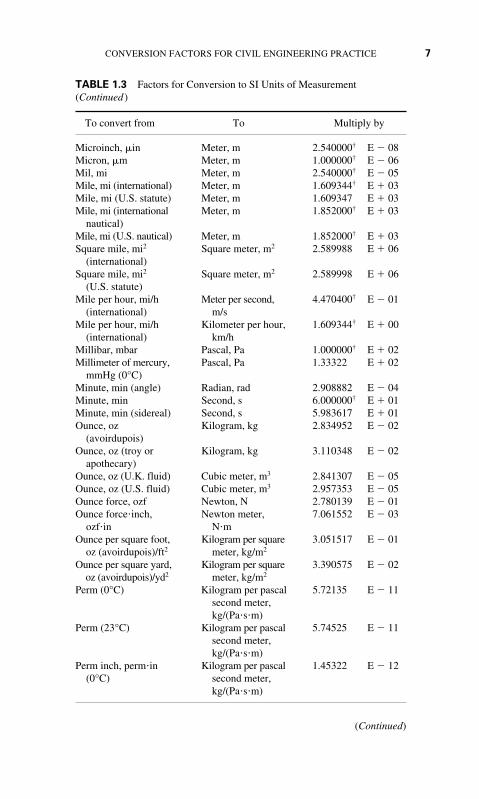
TABLE 1.3 Factors for Conversion to SI Units of Measurement
To convert from To Multiply by
Acre foot, acre ft Cubic meter, m3 1.233489 E � 03Acre Square meter, m2 4.046873 E � 03Angstrom, Å Meter, m 1.000000* E � 10Atmosphere, atm Pascal, Pa 1.013250* E � 05
(standard)Atmosphere, atm Pascal, Pa 9.806650* E � 04
(technical� 1 kgf/cm2)
Bar Pascal, Pa 1.000000* E � 05Barrel (for petroleum, Cubic meter, m2 1.589873 E � 01
42 gal)Board foot, board ft Cubic meter, m3 2.359737 E � 03British thermal unit, Joule, J 1.05587 E � 03
Btu, (mean)British thermal unit, Watt per meter 1.442279 E � 01
Btu (International kelvin, W/(m�K)Table)�in/(h)(ft2)(°F) (k, thermalconductivity)
British thermal unit, Watt, W 2.930711 E � 01Btu (InternationalTable)/h
British thermal unit, Watt per square 5.678263 E � 00Btu (International meter kelvin,Table)/(h)(ft2)(°F) W/(m2�K)(C, thermalconductance)
British thermal unit, Joule per kilogram, 2.326000* E � 03Btu (International J/kgTable)/lb
British thermal unit, Joule per kilogram 4.186800* E � 03Btu (International kelvin, J/(kg�K)Table)/(lb)(°F)(c, heat capacity)
British thermal unit, Joule per cubic 3.725895 E � 04cubic foot, Btu meter, J/m3
(InternationalTable)/ft3
Bushel (U.S.) Cubic meter, m3 3.523907 E � 02Calorie (mean) Joule, J 4.19002 E � 00Candela per square Candela per square 1.550003 E � 03
inch, cd/in2 meter, cd/m2
Centimeter, cm, of Pascal, Pa 1.33322 E � 03mercury (0°C)
(Continued)

4 CHAPTER ONE
TABLE 1.3 Factors for Conversion to SI Units of Measurement(Continued)
To convert from To Multiply by
Centimeter, cm, of Pascal, Pa 9.80638 E � 01water (4°C)
Chain Meter, m 2.011684 E � 01Circular mil Square meter, m2 5.067075 E � 10Day Second, s 8.640000* E � 04Day (sidereal) Second, s 8.616409 E � 04Degree (angle) Radian, rad 1.745329 E � 02Degree Celsius Kelvin, K TK � tC � 273.15Degree Fahrenheit Degree Celsius, °C tC � (tF � 32)/1.8Degree Fahrenheit Kelvin, K TK � (tF � 459.67)/1.8Degree Rankine Kelvin, K TK � TR /1.8(°F)(h)(ft2)/Btu Kelvin square 1.761102 E � 01
(International meter per watt,Table) (R, thermal K�m2/Wresistance)
(°F)(h)(ft2)/(Btu Kelvin meter per 6.933471 E � 00(International watt, K�m/WTable)�in) (thermalresistivity)
Dyne, dyn Newton, N 1.000000† E � 05Fathom Meter, m 1.828804 E � 00Foot, ft Meter, m 3.048000† E � 01Foot, ft (U.S. survey) Meter, m 3.048006 E � 01Foot, ft, of water Pascal, Pa 2.98898 E � 03(39.2°F) (pressure)
Square foot, ft2 Square meter, m2 9.290304† E � 02Square foot per hour, Square meter per 2.580640† E � 05
ft2/h (thermal second, m2/sdiffusivity)
Square foot per Square meter per 9.290304† E � 02second, ft2/s second, m2/s
Cubic foot, ft3 (volume Cubic meter, m3 2.831685 E � 02or section modulus)
Cubic foot per minute, Cubic meter per 4.719474 E � 04ft3/min second, m3/s
Cubic foot per second, Cubic meter per 2.831685 E � 02ft3/s second, m3/s
Foot to the fourth Meter to the fourth 8.630975 E � 03power, ft4 (area power, m4
moment of inertia)Foot per minute, Meter per second, 5.080000† E � 03
ft/min m/sFoot per second, Meter per second, 3.048000† E � 01
ft/s m/s

CONVERSION FACTORS FOR CIVIL ENGINEERING PRACTICE 5
TABLE 1.3 Factors for Conversion to SI Units of Measurement(Continued)
To convert from To Multiply by
Foot per second Meter per second 3.048000† E � 01squared, ft/s2 squared, m/s2
Footcandle, fc Lux, lx 1.076391 E � 01Footlambert, fL Candela per square 3.426259 E � 00
meter, cd/m2
Foot pound force, ft�lbf Joule, J 1.355818 E � 00Foot pound force per Watt, W 2.259697 E � 02
minute, ft�lbf/minFoot pound force per Watt, W 1.355818 E � 00
second, ft�lbf/sFoot poundal, ft Joule, J 4.214011 E � 02
poundalFree fall, standard g Meter per second 9.806650† E � 00
squared, m/s2
Gallon, gal (Canadian Cubic meter, m3 4.546090 E � 03liquid)
Gallon, gal (U.K. Cubic meter, m3 4.546092 E � 03liquid)
Gallon, gal (U.S. dry) Cubic meter, m3 4.404884 E � 03Gallon, gal (U.S. Cubic meter, m3 3.785412 E � 03
liquid)Gallon, gal (U.S. Cubic meter per 4.381264 E � 08
liquid) per day second, m3/sGallon, gal (U.S. Cubic meter per 6.309020 E � 05
liquid) per minute second, m3/sGrad Degree (angular) 9.000000† E � 01Grad Radian, rad 1.570796 E � 02Grain, gr Kilogram, kg 6.479891† E � 05Gram, g Kilogram, kg 1.000000† E � 03Hectare, ha Square meter, m2 1.000000† E � 04Horsepower, hp Watt, W 7.456999 E � 02
(550 ft�lbf/s)Horsepower, hp Watt, W 9.80950 E � 03
(boiler)Horsepower, hp Watt, W 7.460000† E � 02
(electric)horsepower, hp Watt, W 7.46043† E � 02
(water)Horsepower, hp (U.K.) Watt, W 7.4570 E � 02Hour, h Second, s 3.600000† E � 03Hour, h (sidereal) Second, s 3.590170 E � 03
Inch, in Meter, m 2.540000† E � 02
(Continued)

6 CHAPTER ONE
TABLE 1.3 Factors for Conversion to SI Units of Measurement(Continued)
To convert from To Multiply by
Inch of mercury, in Hg Pascal, Pa 3.38638 E � 03(32°F) (pressure)
Inch of mercury, in Hg Pascal, Pa 3.37685 E � 03(60°F) (pressure)
Inch of water, in Pascal, Pa 2.4884 E � 02H2O (60°F) (pressure)
Square inch, in2 Square meter, m2 6.451600† E � 04Cubic inch, in3 Cubic meter, m3 1.638706 E � 05
(volume or sectionmodulus)
Inch to the fourth Meter to the fourth 4.162314 E � 07power, in4 (area power, m4
moment of inertia)Inch per second, in/s Meter per second, 2.540000† E � 02
m/sKelvin, K Degree Celsius, °C tC � TK � 273.15Kilogram force, kgf Newton, N 9.806650† E � 00Kilogram force meter, Newton meter, 9.806650† E � 00
kg�m N�mKilogram force second Kilogram, kg 9.806650† E � 00
squared per meter,kgf�s2/m (mass)
Kilogram force per Pascal, Pa 9.806650† E � 04square centimeter,kgf/cm2
Kilogram force per Pascal, Pa 9.806650† E � 00square meter, kgf/m2
Kilogram force per Pascal, Pa 9.806650† E � 06square millimeter,kgf/mm2
Kilometer per hour, Meter per second, 2.777778 E � 01km/h m/s
Kilowatt hour, kWh Joule, J 3.600000† E � 06Kip (1000 lbf) Newton, N 4.448222 E � 03Kipper square inch, Pascal, Pa 6.894757 E � 06
kip/in2 ksiKnot, kn (international) Meter per second, m/s 5.144444 E � 01Lambert, L Candela per square 3.183099 E � 03
meter, cd/m2
Liter Cubic meter, m3 1.000000† E � 03Maxwell Weber, Wb 1.000000† E � 08Mho Siemens, S 1.000000† E � 00
CONVERSION FACTORS FOR CIVIL ENGINEERING PRACTICE 7
TABLE 1.3 Factors for Conversion to SI Units of Measurement(Continued)
To convert from To Multiply by
Microinch, �in Meter, m 2.540000† E � 08Micron, �m Meter, m 1.000000† E � 06Mil, mi Meter, m 2.540000† E � 05Mile, mi (international) Meter, m 1.609344† E � 03Mile, mi (U.S. statute) Meter, m 1.609347 E � 03Mile, mi (international Meter, m 1.852000† E � 03
nautical)Mile, mi (U.S. nautical) Meter, m 1.852000† E � 03Square mile, mi2 Square meter, m2 2.589988 E � 06
(international)Square mile, mi2 Square meter, m2 2.589998 E � 06
(U.S. statute)Mile per hour, mi/h Meter per second, 4.470400† E � 01
(international) m/sMile per hour, mi/h Kilometer per hour, 1.609344† E � 00
(international) km/hMillibar, mbar Pascal, Pa 1.000000† E � 02Millimeter of mercury, Pascal, Pa 1.33322 E � 02
mmHg (0°C)Minute, min (angle) Radian, rad 2.908882 E � 04Minute, min Second, s 6.000000† E � 01Minute, min (sidereal) Second, s 5.983617 E � 01Ounce, oz Kilogram, kg 2.834952 E � 02
(avoirdupois)Ounce, oz (troy or Kilogram, kg 3.110348 E � 02
apothecary)Ounce, oz (U.K. fluid) Cubic meter, m3 2.841307 E � 05Ounce, oz (U.S. fluid) Cubic meter, m3 2.957353 E � 05Ounce force, ozf Newton, N 2.780139 E � 01Ounce force�inch, Newton meter, 7.061552 E � 03
ozf�in N�mOunce per square foot, Kilogram per square 3.051517 E � 01
oz (avoirdupois)/ft2 meter, kg/m2
Ounce per square yard, Kilogram per square 3.390575 E � 02oz (avoirdupois)/yd2 meter, kg/m2
Perm (0°C) Kilogram per pascal 5.72135 E � 11second meter,kg/(Pa�s�m)
Perm (23°C) Kilogram per pascal 5.74525 E � 11second meter,kg/(Pa�s�m)
Perm inch, perm�in Kilogram per pascal 1.45322 E � 12(0°C) second meter,
kg/(Pa�s�m)
(Continued)

8 CHAPTER ONE
TABLE 1.3 Factors for Conversion to SI Units of Measurement(Continued)
To convert from To Multiply by
Perm inch, perm�in Kilogram per pascal 1.45929 E � 12(23°C) second meter,
kg/(Pa�s�m)Pint, pt (U.S. dry) Cubic meter, m3 5.506105 E � 04Pint, pt (U.S. liquid) Cubic meter, m3 4.731765 E � 04Poise, P (absolute Pascal second, 1.000000† E � 01
viscosity) Pa�sPound, lb Kilogram, kg 4.535924 E � 01
(avoirdupois)Pound, lb (troy or Kilogram, kg 3.732417 E � 01
apothecary)Pound square inch, Kilogram square 2.926397 E � 04
lb�in2 (moment of meter, kg�m2
inertia)Pound per foot� Pascal second, 1.488164 E � 00
second, lb/ft�s Pa�sPound per square Kilogram per square 4.882428 E � 00
foot, lb/ft2 meter, kg/m2
Pound per cubic Kilogram per cubic 1.601846 E � 01foot, lb/ft3 meter, kg/m3
Pound per gallon, Kilogram per cubic 9.977633 E � 01lb/gal (U.K. liquid) meter, kg/m3
Pound per gallon, Kilogram per cubic 1.198264 E � 02lb/gal (U.S. liquid) meter, kg/m3
Pound per hour, lb/h Kilogram per 1.259979 E � 04second, kg/s
Pound per cubic inch, Kilogram per cubic 2.767990 E � 04lb/in3 meter, kg/m3
Pound per minute, Kilogram per 7.559873 E � 03lb/min second, kg/s
Pound per second, Kilogram per 4.535924 E � 01lb/s second, kg/s
Pound per cubic yard, Kilogram per cubic 5.932764 E � 01lb/yd3 meter, kg/m3
Poundal Newton, N 1.382550 E � 01Pound�force, lbf Newton, N 4.448222 E � 00Pound force foot, Newton meter, 1.355818 E � 00
lbf�ft N�mPound force per foot, Newton per meter, 1.459390 E � 01
lbf/ft N/mPound force per Pascal, Pa 4.788026 E � 01
square foot, lbf/ft2
Pound force per inch, Newton per meter, 1.751268 E � 02lbf/in N/m
Pound force per square Pascal, Pa 6.894757 E � 03inch, lbf/in2 (psi)

CONVERSION FACTORS FOR CIVIL ENGINEERING PRACTICE 9
TABLE 1.3 Factors for Conversion to SI Units of Measurement(Continued)
To convert from To Multiply by
Quart, qt (U.S. dry) Cubic meter, m3 1.101221 E � 03Quart, qt (U.S. liquid) Cubic meter, m3 9.463529 E � 04Rod Meter, m 5.029210 E � 00Second (angle) Radian, rad 4.848137 E � 06Second (sidereal) Second, s 9.972696 E � 01Square (100 ft2) Square meter, m2 9.290304† E � 00Ton (assay) Kilogram, kg 2.916667 E � 02Ton (long, 2240 lb) Kilogram, kg 1.016047 E � 03Ton (metric) Kilogram, kg 1.000000† E � 03Ton (refrigeration) Watt, W 3.516800 E � 03Ton (register) Cubic meter, m3 2.831685 E � 00Ton (short, 2000 lb) Kilogram, kg 9.071847 E � 02Ton (long per cubic Kilogram per cubic 1.328939 E � 03
yard, ton)/yd3 meter, kg/m3
Ton (short per cubic Kilogram per cubic 1.186553 E � 03yard, ton)/yd3 meter, kg/m3
Ton force (2000 lbf) Newton, N 8.896444 E � 03Tonne, t Kilogram, kg 1.000000† E � 03Watt hour, Wh Joule, J 3.600000† E � 03Yard, yd Meter, m 9.144000† E � 01Square yard, yd2 Square meter, m2 8.361274 E � 01Cubic yard, yd3 Cubic meter, m3 7.645549 E � 01Year (365 days) Second, s 3.153600† E � 07Year (sidereal) Second, s 3.155815 E � 07
*Commonly used in engineering practice.†Exact value.From E380, “Standard for Metric Practice,” American Society for Testing and
Materials.

This page intentionally left blank

CHAPTER 2BEAM
FORMULAS
In analyzing beams of various types, the geometric properties of a variety ofcross-sectional areas are used. Figure 2.1 gives equations for computing area A,moment of inertia I, section modulus or the ratio S � I/c, where c � distancefrom the neutral axis to the outermost fiber of the beam or other member. Unitsused are inches and millimeters and their powers. The formulas in Fig. 2.1 arevalid for both USCS and SI units.
Handy formulas for some dozen different types of beams are given in Fig. 2.2.In Fig. 2.2, both USCS and SI units can be used in any of the formulas that areapplicable to both steel and wooden beams. Note that W � load, lb (kN); L �length, ft (m); R � reaction, lb (kN); V � shear, lb (kN); M � bending moment,lb � ft (N � m); D � deflection, ft (m); a � spacing, ft (m); b � spacing, ft (m);E � modulus of elasticity, lb/in2 (kPa); I � moment of inertia, in4 (dm4); � �less than; � greater than.
Figure 2.3 gives the elastic-curve equations for a variety of prismatic beams.In these equations the load is given as P, lb (kN). Spacing is given as k, ft (m)and c, ft (m).
CONTINUOUS BEAMS
Continuous beams and frames are statically indeterminate. Bending moments inthese beams are functions of the geometry, moments of inertia, loads, spans,and modulus of elasticity of individual members. Figure 2.4 shows how anyspan of a continuous beam can be treated as a single beam, with the momentdiagram decomposed into basic components. Formulas for analysis are given inthe diagram. Reactions of a continuous beam can be found by using the formu-las in Fig. 2.5. Fixed-end moment formulas for beams of constant moment ofinertia (prismatic beams) for several common types of loading are given in Fig. 2.6.Curves (Fig. 2.7) can be used to speed computation of fixed-end moments inprismatic beams. Before the curves in Fig. 2.7 can be used, the characteristicsof the loading must be computed by using the formulas in Fig. 2.8. Theseinclude xL, the location of the center of gravity of the loading with respectto one of the loads; G2 � b2
n Pn/W, where bnL is the distance from eachload Pn to the center of gravity of the loading (taken positive to the right); and
1111

A = bd
bd
b2 + d2
c1 = d/2
S1 =
c1
1
3 c3
2b
b
Rectangle Triangle
1d
d
23
33
c1
c2
b
Half ParabolaParabola
dc1
11
22
c
2
1 1
2
1
2b
1
d
2
c2 = d
c3 =
bd2
6l1 = bd3
36
S1 = bd2
24
c1 = 2d3
A = bd23
l2 = bd3
12
r1 = d18r1 = d
12
l1 = bd3
12
l2 = bd3
3
l3 =
S3 =
b3d3
b2d2
6 (b2 + d2)
b2 + d26
r3 = bd
6 (b2 + d2)
l1 = bd3
bd
8175
l3 = 16105
l2 = b3d30
A = bd23
l1 = bd38175
l2 = b3d19480
A = bd2
c = d35
c1 = d35
c2 = b58
12

FIGURE 2.1 Geometric properties of sections.
Section
Equilateral polygonA = Area
r = Rad inscribed circlen = No. of sidesa = Length of sideAxis as in preceding sectionof octagon
R = Rad circumscribed circle
Moment of inertia
b1 b12 2
c
b
h
I = (6R2 − a2)6R2 − a2
24
12r2 + a2
48
12b2 + 12bb1 + 2b12
6 (2b + b1)
R2
≈
A24
= Ir
Ic
I = h36b2 + 6bb1 + b12
36 (2b + b1)
=180°
n
I
R cos
c = h3b + 2b12b + b1
= h2 h6b2 + 6bb1 + b12
12 (3b + 2b1)Ic
= (12r2 + a2)A48
= (approx)AR2
4 = (approx)AR4
Section modulus Radius of gyration
13
13

b2
b2
b2
b2
B2
B2
hH H Hh h
c
h
c
h hH
H H
BbB
b
b b
B B B
BH3 + bh3
12
BH3 – bh3
12
BH3 + bh3
6H
BH3 – bh3
6H
=I
Ic =
=I
=
BH3 + bh3
12 (BH + bh)
BH3 – bh3
12 (BH – bh)Ic
Section Moment of inertia Section modulus Radius of gyration
14

FIGURE 2.1 (Continued)
b2
HH HH
h
h
h 1
b
c 2 a
a a a2
a2
b
B
B Bb
B
c 1d 1
B12
d
d d d
b2
b2
c 2c 1
c 2c 1
hd
I(Bd + bd1) + a (h + h1)
r =
c2 = II – c1
I = (Bc13 – bh3 + ac2
3)
c1 =
I[Bd + a (II – d)]
ali2 + bd2
ali + bd
I = (Bc13 – B1h3 + bc2
3 – b1h13)
c1 =aH2 + B1d2 + b1d1 (2H – d1)
aH + B1d + b1d1
12
13
1212
Section Moment of inertia and section modulus Radius of gyration
B12
15

R
rr
d
dm = (D + d)
(D4 – d4)
s = (D – d)
D
d
R4 + r2
2
I = π64
I = r2=πd4
64πr4
4= A
4
(R4 – r4)= π4A4
(R2 + r2)=
= 0.05 (D4 – d4) (approx)
D4 – d4
Dπ32
D2 + d2
2
R4 – r4
R=
=
π4
when is very small
= 0.8dm2s (approx)
0.05d4 (approx)=
r=πd3
32πr3
4= A
4
1212
Ic
0.1d3 (approx)=
=
Ic =
d4
r2
sdm
=
Section Moment of inertia Radius of gyrationSection modulus
16

FIGURE 2.1 (Continued)
17
c 2c 2
c 1c 1
r
r
r1R
I = r4
I = 0.1098 (R4 – r4)
= 0.3tr13 (approx)
when is very small
0.283R2r2 (R – r)R + r
π8
89π
_
= 0.1098r4
–
tr1
Ic2
Ic1c1
= 0.1908r3
= 0.2587r3
= 0.4244r
c1 =
c2 = R – c1
43π
R2 + Rr + r2
R + r
9π2 – 646π
r = 0.264r
2Iπ (R2 – r2)
= 0.31r1 (approx)t
a 1
a
a
t
t
b1 b
b
(approx)
(approx)
(approx)
I = 0.7854a3b=πa3b4
(a3b – a13b1)
= 0.7854a2b=πa2b4
I = π4
a (a + 3b)t= π4
Ic
Ic
a2
a2
a + 3ba + b
I(πab – a1b1)
a2 (a + 3b)t==
π4

18
B 4B 4
B2
bb
d
B2
Hh
h
B
(approx)
I = l12
B2
I = ++t4
t
23
3π16
Ic
2 + hπB4
π
I
Section Moment of inertia and section modulus Radius of gyration
+ B2h h3
h = H –
πB3
16πBh2
2
+ 2b (h – d)d2
4
d4 + b (h3 – d3) + b3 (h – d) I
= l6h
Ic
= 2IH + t
3π16
d4 + b (h3 + d3) + b3 (h – d)
t
b2
h 2 h 1
H
BCorrugated sheet iron,parabolically curved
t
b1
3It (2B + 5.2H)
r =
I =
=
h1 =
(b1h13 – b2h2
3), where
(H + t)
h2 = (H – t)
64105
2IH + t
Ic
1212
1414
b1 = (B + 2.6t)
b2 = (B – 2.6t)
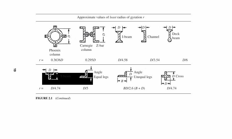
FIGURE 2.1 (Continued)
Approximate values of least radius of gyration r
DD
D D DD Cross
DB
D D D
D
CarnegiecolumnPhoenix
column
r =
r =
0.3636D 0.295D D/4.58
BD/2.6 (B + D) D/4.74D/4.74 D/5
D/3.54 D/6
Z-bar
I-beam
T-beam
Channel
AngleUnequal legs
AngleEqual legs
Deckbeam
19
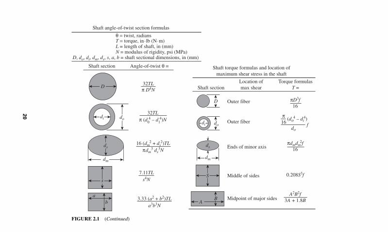
FIGURE 2.1 (Continued)
D
dm
ds
dm
ab
s
do
D Outer fiber
Shaft section
Shaft torque formulas and location ofmaximum shear stress in the shaft
Shaft section
Shaft angle-of-twist section formulas
Angle-of-twist θ =
D, do, di, dm, ds, s, a, b = shaft sectional dimensions, in (mm)N = modulus of rigidity, psi (MPa)L = length of shaft, in (mm)T = torque, in.lb (N.m)θ = twist, radians
Location ofmax shear
Torque formulasT =
Outer fiber
Ends of minor axis
Middle of sides
Midpoint of major sides
32TLπ D4N
πD3f16
πdmdm2f
16
f
π16
0.208S3f
A2B2f3A + 1.8B
32TLπ (d0
4 – d14)N
di
7.11TLs4N
3.33 (a2 + b2)TLa3b3N
16 (dm2 + ds
2)TLπdm
3 ds3N
(do4 – di
4)
do
S
AB
di
ds
do
20

CASE 2. Beam Supported Both Ends—Concentrated Load at Any Point
R = WbL
WaL
R1 =
V (max) = R when a < b and R1 when a > b
At point of load:At x: when x = a (a + 2b) + 3 and a > b
D (max) = Wab (a + 2b) 3a (a + 2b) + 27 EIL
At x: when x < a
At x: when x > a
At x: when x < a
L W
DR R1
Mx
V
a b
At x: WbL
V =
WabL
M (max) =
WbxL
M =
Wbx6 EIL
D = 2L (L – x) – b2 – (L – x)2
Wa (L – x)6 EIL
D = 2Lb – b2 – (L – x)2
FIGURE 2.2 Beam formulas. (From J. Callender, Time-Saver Standards for Architectural Design Data, 6th ed., McGraw-Hill, N.Y.)
21

CASE 3. Beam Supported Both Ends—Two Unequal Concentrated Loads, Unequally Distributed
R = 1L
W (L – a) + W1b M = aL
W (L – a) + W1b
M1 = bL
Wa + W1 (L – b)
M = W aL
bxL
(L – x) + W1
R1 = 1L
Wa + W1 (L – b)
V (max) = Maximum reaction
At point of load W:
At point of load W1:
At x: when x > a or < (L – b)At x: when x > a and < (L – b)
V = R – W
R
Wa
x
Lb
W1
M M1
V
R1
22

23
FIGURE 2.2 (Continued)
CASE 4. Beam Supported Both Ends—Three Unequal Concentrated Loads, Unequally Distributed
R =Wb + W1b1 + W2b2
L
R1 =
V (max) = Maximum reaction
At x: when x > a and < a1
At x: when x = a
At x: when x = a1
M = Ra
M1 = Ra1 – W (a1 – a)At x: when x = a2
M2 = Ra2 – W (a2 – a) – W1 (a2 – a1)M (max) = M when W = R or > R
M (max) = M1 when
M (max) = M2 when W2 = R1 or > R1
La2
W2W1W
R
M
V
xR1
M1M2
b2b1ba
W1 + W = R or > RW1 + W2 = R1 or > R1
At x: when x > a1 and < a2
V = R – W
V = R – W – W1
Wa + W1a1 + W2a2L
a1

DR1
At center:
At supports:
At x:
At x:
R
V
V
W
x
L
M
M1
M (max) =
(L2 – 2Lx + x2)
WL24
M1 (max) = WL12
L2
6M = – + Lx – x2W
2L
At center:
At x:
D (max) =1
384WL3
EI
D =Wx2
24 EIL
R = R1 = V (max) =W2
V = –W2
WxL
CASE 5. Beam Fixed Both Ends—Continuous Load, Uniformly Distributed
24

FIGURE 2.2 (Continued)
25
CASE 6. Beam Fixed Both Ends—Concentrated Load at Any Point
b2 (3a + b)L3
V (max) = R when a < b= R1 when a > b
At x: when x =
when x < a
At x: when x < a
At support R:
At support R1:
At x:
At point of load:
R1 = W
R = W M1 = – W
V = R
a2 (3b + a)L3
ab2
L2 and a > b2 aL3a + b
2 W a3b2
3 EI (3a + b)2
a
x
WL
DR1
M1 M2
M
V
b
R
max neg. mom.when b > a
M2 = – W a2bL2
M (max) = Ra + M1 = Ra – W
D (max) =
W b2x2
6 EIL3D = (3aL – 3ax – bx)M = Rx – W
ab2
L2ab2
L2
max neg. mom.when a > b

R1Loading
At fixed end: At free end:
At x:At x:
Bending
Shear
D
V
W
x
L
M
M (max) =
(x4 – 4L3x + 3L4)
WL2
M = Wx2
2L
At x:
D (max) =WL3
8EI
D =W
24EIL
R1 = V (max) = W
V =WxL
CASE 7. Beam Fixed at One End (Cantilever)—Continuous Load, Uniformly Distributed
26

FIGURE 2.2 (Continued)
27
DR1
V
W
x
a b
L
M
CASE 8. Beam Fixed at One End (Cantilever)—Concentrated Load at Any Point
R1 = V (max) = W
M (max) = Wb
M = W (x = a)
At x: when x > a
At fixed end:
At free end:
At x: when x < aAt x: when x > a
At x: when x > a
V = W
V = 0
WL3
6EI33a
LD (max) = 2 – a
L+
W6EI
–3aL2 + 2L3 + x3
–3ax2 – 3L2x + 6aLxD =
At point of load:W
3EID = (L – a)3

At x: when x < a
At x: when x > aAt x: when x > a
At x: when x = a = 0.414L
At x: when x < a
At x: when x > a
At x: when x < a
At point of load:
At fixed end:
V = R
V = R – W
R1 = W 3aL2 – a3
2L3
16EI
R = W 3b2L – b3
2L3
3RL2x – Rx3 –
R1(2L3 – 3L2x + x3) –
3b2L – b3
2L3
a
x
WL
DR1
M1
M
V
b
R
M (max) = Wa D (max) = 0.0098
D =
16EI
D =
3b2L – b3
2L3M = Wx
3b2L – b3
2L3M = Wx
3b2L – b3
2L3
WL3
EI
M1 (max) = WL – W (L – a)
– W (x – a)
CASE 9. Beam Fixed at One End, Supported at Other—Concentrated Load at Any Point
3 W (L – a)2 x
3 Wa (L – x)2
28

FIGURE 2.2 (Continued)
29
D
At fixed end:
At x:
At x: when x =At x: when x = 0.4215L
At x:
R R1
V
W
x
L
M
M1
M (max) = WL9
128
M1 (max) =
M = xL – WxL
WL18
38
12
L38
At x:
D (max) = 0.0054WL3
EI
D =Wx
48EIL
R1 = V (max) =58 W
R = 38 W
V = W –38
WxL
CASE 10. Beam Fixed at One End, Supported at Other—Continuous Load, Uniformly Distributed
– 3Lx2 + 2x3 + L3

At x: when x < a
At x1: when x1 < LAt x1: when x1 < L V = R – w (a + x1)
At x2: when x2 < b V = w (b – x2)
At x: when x < a V = w (a – x)
At x2: when x2 < b
At x1: when x1 =
At R:
At R1:
a
x x1 x2
W
LR1
M1
M1
M
bR
– a
wa212
R2w
= W = load per unit of lengthWa + L + b
– aRw
M (max) = R
V (max) = wa or R – wa
M1 =
w (a – x)212
M =
w (a + x1)2 – Rx112
M =
w (b – x2)212
M =
wb212
M1 =
R = w [(a + L)2 + b2]2L
R1 = w [(b + L)2 + a2]2L
CASE 11. Beam Overhanging Both Supported Unsymmetrically Placed—Continuous Load, Uniformly Distributed
30

FIGURE 2.2 (Continued)
31
D
D
V V
R1
At x1: when x1 < L
At x: when x < aAt x: when x < a
R
W2
x
a aL
x1
M (max) =
(a – x)
Wa2
M
M =W2
At center:
At free ends:D =
Wa2 (3L + 2a)12EI
D =WaL2
16EI
R = R1 = V (max) =W2
V =W2
CASE 12. Beam Overhanging Both Supports, Symmetrically Placed—Two Equal Concentrated Loads at Ends
W2

L
Load
x(l – x)wL2
x(l – 2x2 + x3)
– x wL
Shear
Moment
Elastic curve
(a)
w
xL
R =
R
R
wL2
R = wL2
wL2
8
wL3
24EI
5wL4
384EI
wL4
24EI
L2
12
12
12
x <12
cL
L
Load
a +
(2c + b)
(x′ < a) (x″ < c)
Shear
Moment
(b)
b
w
a c
R =
R2
R1
wb2L
(2c + b)R2 = wb2L
R1w
R1
2w
R1 – w (x – a)
w 2
x(a < x < a + b)
(x –
a)2
–
x′ x″
R1x′ R1x R
1(a
+
R2x″
R1a R2c
L
Load
k(1 – k)PL
k(1 – k)(2 – k)
Shear
Moment
Elastic curve
(c)
P
R2
R1
R1 = (l – k)P R2 = Pk
PL2
6EI
12
32
k(1 – k2)
1 – k2
3
PL2
6EI
k2(1 – k)2PL3
3EIk=dmax 1 – k2
3PL3
3EI
kx″(1 – k2 – x″2)PL3
6EI(1 – k)x′(2k – k2 – x′2)
PL3
6EI
k <(l – k)L
x′L(x′ < k)
R2 x″ LR1 x′ L
L
x″L(x″ < (1 – k))
kL
32
FIGURE 2.3 Elastic-curve equations for prismatic beams: (a) Shears, moments, and deflections for full uniform load on a simply sup-ported prismatic beam. (b) Shears and moments for uniform load over part of a simply supported prismatic beam. (c) Shears, moments,and deflections for a concentrated load at any point of a simply supported prismatic beam.

33
P
P
P P
L
Load
(1 – 2k)L
PxL
x(3k – 3k2 – x2)
k(3x′ – 3x′2 – k2)
k(3 – 4k2)
Shear
Moment
Elastic curve(e)
xL(x < k)
k(1 – k)PL2
2EI
PL3
6EI
PL3
24EI
PkL
PL3
6EI
L2
L′′2
kL kL
R = PR = P
x′(k < x′ < (1 – k))
P
PR P P
P
P
P P PPaLaLaLaLaLaL
(For n aneven number)
(For n an even number)
Load
maL
Shear
Moment
Elastic curve
(f)
L
R
W = np
(n + 1)(For n an odd number)
PL8
n(n + 2)n + 1
PL8
L2
L2
L2
L2
nPR =a =
12
nPR = 12
1n + 1
n(n + 2)n + 1
PL2
24EIn(n + 2)PL3
384EI(5n2 + 10n + 6)
(n + 1)3
(For n an odd number)PL3
384EI5n2 + 10n + 1
n + l
m(n – m + 1)n + 1
PL2
cL
P/2
P/2
P
L
Load
xPL
x(3 – 4x2)
Shear
Moment
Elastic curve
(d)
xL
PL2
16EIPL3
48EI
PL4
PL3
48EI
12
L2
L2
PR = 12
PR = 12
x < 12
cL
FIGURE 2.3 Elastic-curve equations for prismatic beams: (d) Shears, moments, and deflections for a concentrated load at midspan of a simply supportedprismatic beam. (e) Shears, moments, and deflections for two equal concentrated loads on a simply supported prismatic beam. ( f ) Shears, moments, and deflec-tions for several equal loads equally spaced on a simply supported prismatic beam. (Continued)

P
P
Load
Shear
Moment
Elastic curve
(g)
PR1 =L′L
L′
xPL′
x′L′xL
Px′L′PL′
L
PR2 =
R2
R1
L + L′L
2(L + L′) – L′x′ (1 + x′)
L3
(L + L′)PL′23EIx(1 – x2)PL′L2
6EIPL′2 (1 – x′)
6EI
dmax = PL′L2
3EI9
P
PL
Load
Shear
Moment
Elastic curve
(h)
R = P
LP
PL
xL
PxL
R
(2 – 3x + x3)PL3
3EI
PL3
3EI
L L′
Load
(L2 – L′2)
xL
wL′x′wL′
Shear
Moment
Elastic curve
(i)
ww
R1 =
R1
R2
w2L
R1 = wLx
R2 = w2L
(L2 – L′2)w2L
(L + L′)2 (L – L′)2w
8L2
wL2x24EI
wL′24EI
wL′22 x′2wL′2
2
L2
1 –
(L2 – L′2 – xL2)
L2 (1 – 2x2 + x2) –2L′2(1 – x2)
(4L′2 – L3 + 3L′3)
wx2
L′2
L2L 1 –
(L + L′)2
x′L′
L′2
L2
34
FIGURE 2.3 Elastic-curve equations for prismatic beams: (g) Shears, moments, and deflections for a concentrated load on a beam overhang. (h) Shears,moments, and deflections for a concentrated load on the end of a prismatic cantilever. (i) Shears, moments, and deflections for a uniform load over the fulllength of a beam with overhang. (Continued)

35
Load
Shear
Moment
Elastic curve
(j)
R = wL
wLx
wL
xL
L
w
wL2
2
wL2
2
(3 – 4x + x4)
x2
wL4
24EI
wL4
8EI
wL212
Load
Shear
Moment
Elastic curve
(k)
R1 =
R2R1
wL′
wL′x′
x′L′
xL
L L′w
wL′22L
R2 =wL′2L
wL′22
L3
(4L + 3L′)x(1 – x2)
x′2
wL′324EI
dmax =wL′2L2
wL′2L2
12EI
wL′2x12
wL′212
3EI18
(2L + L′)
Load
Shear
Moment
Elastic curve
(l)
R = W
wW =
Wx2
W
xL
xL
L
wx
WL3
L3
WL3
wL2
WL3
(4 – 5x + x3)
x3
WL3
60EI
WL3
15EI
FIGURE 2.3 Elastic-curve equations for prismatic beams: (j) Shears, moments, and deflections for uniform load over the full length of a cantilever.(k) Shears, moments, and deflections for uniform load on a beam overhang. (l) Shears, moments, and deflections for triangular loading on a prismaticcantilever. (Continued)

Shear
Moment(m)
0.5774l
R1
R1 = V1
R2 = V2max
Mmax
Δmax
Δx
at x = = 0.5774l
Vx
Mx
R2
V1
lx W
Mmax
V2
= W3
W 3
= 2W3
=
=
W3
– Wx2
l2
(l2 – x2)
Wl2
EI
=
= 0.01304
(3x4 – 10l2x2 + 7l4)Wx180EIl2
=
Wx3l2
= 0.1283Wl2Wl
at x = l 1 – = 0.5193l815
39
36
FIGURE 2.3 Elastic-curve equations for prismatic beams. (m) Simple beam—load increasing uniformly to one end.(Continued)
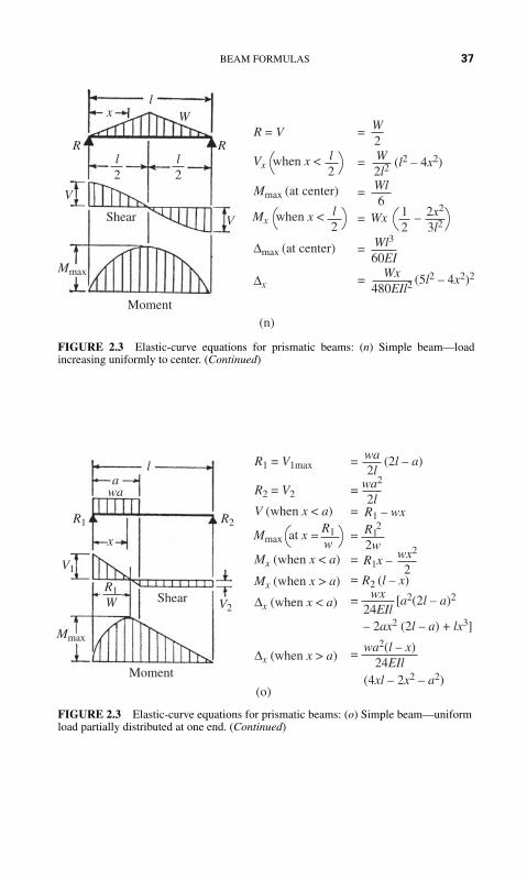
BEAM FORMULAS 37
Shear
Moment(n)
R = V
Mmax (at center)
Δmax (at center)
Δx
R
V
R
x Wl
V
Mmax
= (l2 – 4x2)W2l2
= W2
= Wl6
(5l2 – 4x2)2Wx480EIl2
=
l2
l2
Vx
Mx
when x < l2
= Wx –when x < l2
2x2
3l212
= Wl3
60EI
Shear
Moment
(o)
R1 = V1max (2l – a)
Mmax
R2R1
R1W V2
awa
x
l
V1
Mmax
=
wx2
2
R2 = V2
R1 – wx
= wa2
2l
wa2l
=
=
wx24EIl
=
V (when x < a)
R1x –=
R2 (l – x)=
Mx (when x < a)
Mx (when x > a)
[a2(2l – a)2=Δx (when x < a)
wa2(l – x)24EIl
(4xl – 2x2 – a2)
=Δx (when x > a)
R1w
R12
2wat x
– 2ax2 (2l – a) + lx3]
FIGURE 2.3 Elastic-curve equations for prismatic beams: (n) Simple beam—loadincreasing uniformly to center. (Continued)
FIGURE 2.3 Elastic-curve equations for prismatic beams: (o) Simple beam—uniformload partially distributed at one end. (Continued)

38 CHAPTER TWO
Shear
Moment
(p)
R = V = P= Pl
= Px
=
Mmax (at fixed end)
Δmax (at free end)
Δx
Mx
R
P
V
x
l
Mmax
Pl3
3EI
= P6EI
(2l3 – 3l2x + x3)
Shear
Moment(q)
R = V
Mmax (at center and ends)
Δmax (at center)
Δx
R
P
V
xl
V
R
Mmax
MmaxMmax
= P2
= (4x – l)P8
=
(3l – 4x)
Pl3
192EI
= Px2
48EI
= Pl8
l4
l2
l2
Mx when x < l2
FIGURE 2.3 Elastic-curve equations for prismatic beams: (p) Cantilever beam—con-centrated load at free end. (Continued)
FIGURE 2.3 Elastic-curve equations for prismatic beams: (q) Beam fixed at bothends—concentrated load at center. (Continued)

P
P
R
L
L R
A L
L R L R L R
R
(a)
(b)
(c)
ML
ML ML MRMR
MR
kL
VRVL
kL kLk(l – k)PL
+ +=
k(l – k)PL
B C
FIGURE 2.4 Any span of a continuous beam (a) can be treated as a simple beam, as shown in(b) and (c). In (c), the moment diagram is decomposed into basic components.
39

40 CHAPTER TWO
R1
d1
y11
d1 = y11R1 + y12R2 + y13R3d2 = y21R1 + y22R2 + y23R3d3 = y31R1 + y32R2 + y33R3
y21
y31
d2
d3
R0
L1 L2
W
L3 L4
R2 R3 R4
(a)
(b)
(c)
y13
1
1
1
y23 y33
y12 y22
y32
(e)
(d)
FIGURE 2.5 Reactions of continuous beam (a) found by makingthe beam statically determinate. (b) Deflections computed with inte-rior supports removed. (c), (d ), and (e) Deflections calculated forunit load over each removed support, to obtain equations for eachredundant.

BEAM FORMULAS 41
kL
kL
kL kL
kL
–k(l – k)2 WL
k(l – k)WL
k(l – k)WL
k2(l – k)WL
W
L
L L
(a) (b)
(c) (d)
w
L
WL12
WL12
L2
WL
W = wL
L4
L4
L4
L4
18
WL18 WL
18
WL16
WL5
48
WL5
48
W13
12
k(l – k)WL12
kWL12
W2
W2
W13
W13
–
–
– Lc
FIGURE 2.6 Fixed-end moments for a prismatic beam. (a) For a concentrated load.(b) For a uniform load. (c) For two equal concentrated loads. (d) For three equal concentrated loads.

42 CHAPTER TWO
0 0.05 0.10 0.15
m =MF
WL
WaL
0.20
01.0
0.10.9
0.20.8
G 2 = 0.05
G2 = 0
G2 =
0G 2 = 0.15
G 2 = 0.20
G 2 = 0.25
0.30.7
a
0.40.6
Use upper line for MRF
Use lower line for MLF
0.60.4
0.70.3
0.80.2
0.90.1
1.00
0.5
G2 = 0
S3 =
0
S3 =
0.0
5 fo
r m R
(–0.
05fo
r m L
)
S3 =
–0.
05 fo
r m R
(0.0
5fo
r m L
)
G 2 = 0.10
G2 = 0.10
FIGURE 2.7 Chart for fixed-end moments due to any type of loading.

BEAM FORMULAS 43
W = P
W = wyL
W =
W = (n + 1)P
nPyL
xL
xL
yL
w
yL
xL
w
X = 0 x = yn1 + nG2 = 0
G2 =S3 = 0
S3 = 0
Case 1
Case 3 Case 4
Case 2
P
x = y12
y2n(1 + n)2
G2 = y2112
S3 = –
x = y13
G2 = y2118
y31135
S3 = y3n(n – 1)(1 + n)3
wyL2
–
–
–
–
––
–
FIGURE 2.8 Characteristics of loadings.

44 CHAPTER TWO
W =wyL
2
yL
xL
yL yL yL yL yL yL
aL
P P P P P P P
yL
xL
–xL
Ldx
xL
yL
y
0
w
Case 6
G2 = y2 =n2 – 112
n + 1n – 1
LÚ wx′dx′W
y
0W = LÚ f(x′)dx′
a2
12.
S3 = 0
Case 5
S3 = 0
Case 7 Case 8
x =
W = nP
y
yL
12
x =
x =y
0LÚ wx2dx
WG2 =
y
0LÚ wx3dx
WS3 =
yn – 12
12
yL12
G2 = y2124
S3 = –
x =
x =
y14
G2 = y2380
y31160
W =13
wyL
w = ky2L2
W = f(x′)
x′L
–
–
–
–
–
–
–
–
FIGURE 2.8 (Continued)

BEAM FORMULAS 45
S3 � Pn/W. These values are given in Fig. 2.8 for some common typesof loading.
Formulas for moments due to deflection of a fixed-end beam are given inFig. 2.9. To use the modified moment distribution method for a fixed-end beamsuch as that in Fig. 2.9, we must first know the fixed-end moments for a beamwith supports at different levels. In Fig. 2.9, the right end of a beam with span Lis at a height d above the left end. To find the fixed-end moments, we firstdeflect the beam with both ends hinged; and then fix the right end, leaving theleft end hinged, as in Fig. 2.9(b). By noting that a line connecting the two sup-ports makes an angle approximately equal to d/L (its tangent) with the originalposition of the beam, we apply a moment at the hinged end to produce an endrotation there equal to d/L. By the definition of stiffness, this moment equalsthat shown at the left end of Fig. 2.9(b). The carryover to the right end is shownas the top formula on the right-hand side of Fig. 2.9(b). By using the law of
bn3
(a)
(b)
(c)
(d)
dL
L
L
R
R
d
d
d
MRF
MLF
KLF
CRFKL
F
=CLFKR
F
L
dL
dL
KRF
R
L
L
R
dL
dL
CLFKR
F
= CRFKL
F
dLdL
KRF 1 + CL
F dL
KLF 1 + CR
F dL
dL
FIGURE 2.9 Moments due to deflection of a fixed-end beam.

46 CHAPTER TWO
reciprocal deflections, we obtain the end moments of the deflected beam inFig. 2.9 as
(2.1)
(2.2)
In a similar manner the fixed-end moment for a beam with one end hinged andthe supports at different levels can be found from
(2.3)
where K is the actual stiffness for the end of the beam that is fixed; for beams ofvariable moment of inertia K equals the fixed-end stiffness times .
ULTIMATE STRENGTH OF CONTINUOUS BEAMS
Methods for computing the ultimate strength of continuous beams and framesmay be based on two theorems that fix upper and lower limits for load-carryingcapacity:
1. Upper-bound theorem. A load computed on the basis of an assumed linkmechanism is always greater than, or at best equal to, the ultimate load.
2. Lower-bound theorem. The load corresponding to an equilibrium conditionwith arbitrarily assumed values for the redundants is smaller than, or at bestequal to, the ultimate loading—provided that everywhere moments do notexceed MP. The equilibrium method, based on the lower bound theorem, isusually easier for simple cases.
For the continuous beam in Fig. 2.10, the ratio of the plastic moment for theend spans is k times that for the center span (k 1).
Figure 2.10(b) shows the moment diagram for the beam made determinateby ignoring the moments at B and C and the moment diagram for end momentsMB and MC applied to the determinate beam. Then, by using Fig. 2.10(c), equi-librium is maintained when
(2.4)�wL2
4(1 � k)
�wL2
4 � kMP
MP �wL2
4�
1
2MB �
1
2MC
(1 � C LFC R
F)
MF � Kd
L
MRF � K R
F (1 � C LF)
d
L
MFL � K F
L (1 � C FR)
d
L

BEAM FORMULAS 47
The mechanism method can be used to analyze rigid frames of constant sec-tion with fixed bases, as in Fig. 2.11. Using this method with the vertical load atmidspan equal to 1.5 times the lateral load, the ultimate load for the frame is4.8MP/L laterally and 7.2MP /L vertically at midspan.
Maximum moment occurs in the interior spans AB and CD when
(2.5)x �L
2�
M
wL
AB
MB
kMP kMP
kMPkMP
wL2
8
MP
MC
CD
w
L
x x
L
(a)
(b)
(c)
Moment diagramfor redundants
Moment diagramfor determinate beam
L
2ww
wL2
4
wL2
8
FIGURE 2.10 Continuous beam shown in (a) carries twice as much uniformload in the center span as in the side span. In (b) are shown the moment diagramsfor this loading condition with redundants removed and for the redundants. Thetwo moment diagrams are combined in (c), producing peaks at which plastic hingesare assumed to form.

L2
L
B B
A
E E
LD A D
BPC CC
P
(a) (b) Beammechanism
(c) Framemechanism
(d) Combinationmechanism
(e) (f) (g)
A A AD D D
B
P
B BEE
EC C C
A D
BE
C
1.5P
1.5P1.5P
L2
L2
L2
θL2
θL2θL
2
θL2 θ
θ
θ
θ θ
θ
θθ
θ θθ2θ2θ
L2
L2
L2
FIGURE 2.11 Ultimate-load possibilities for a rigid frame of constant section with fixed bases.
48

BEAM FORMULAS 49
or if
(2.6)
A plastic hinge forms at this point when the moment equals kMP. For equilibrium,
leading to
(2.7)
When the value of MP previously computed is substituted,
from which k � 0.523. The ultimate load is
(2.8)
In any continuous beam, the bending moment at any section is equal to thebending moment at any other section, plus the shear at that section times itsarm, plus the product of all the intervening external forces times their respectivearms. Thus, in Fig. 2.12
(2.9)
(2.10)
(2.11)
Table 2.1 gives the value of the moment at the various supports of a uniformlyloaded continuous beam over equal spans, and it also gives the values of the shears
Mx � M3 � V3x � P3a
� P1 (l2 � c � x) � P2 (b � x) � P3a
Mx � R1 (l1 � l2 � x) � R2 (l2 � x) � R3x
Vx � R1 � R2 � R3 � P1 � P2 � P3
wL �4MP (1 � k)
L� 6.1
MP
L
7k2 � 4k � 4 or k (k � 4�7) � 4�7
k2MP2
wL2 � 3kMP �wL2
4� 0
�w
2 � L
2�
kMP
wL � � L
2�
KMP
wL � � � 1
2�
kMP
wL2 � kMP
kMP �w
2x (L � x) �
x
LkMP
M � kMP when x �L
2�
kMP
wL
P2 P3P1
R1l1 l2 l3
x
l4
R2
abcR3 R4 R5
FIGURE 2.12 Continuous beam.

TABLE 2.1 Uniformly Loaded Continuous Beams over Equal Spans(Uniform load per unit length � w; length of each span � l)
Shear on each side Distance to point Notation of support. L � left, of max moment, Distance to
Number of R � right. reaction at Moment Max. measured to point of inflection,of support any support is L � R over each moment in right from measured to right
supports of span L R support each span support from support
2 1 or 2 0 0 0.125 0.500 None
3 1 0 0 0.0703 0.375 0.7502 0.0703 0.625 0.250
4 1 0 0 0.080 0.400 0.8002 0.025 0.500 0.276, 0.7241 0 0 0.0772 0.393 0.786
5 2 0.0364 0.536 0.266, 0.8063 0.0364 0.464 0.194, 0.7341 0 0 0.0779 0.395 0.789
6 2 0.0332 0.526 0.268, 0.7833 0.0461 0.500 0.196, 0.8041 0 0 0.0777 0.394 0.7882 0.0340 0.533 0.268, 0.790
7 3 0.0433 0.490 0.196, 0.7854 0.0433 0.510 0.215, 0.8041 0 0 0.0778 0.394 0.789
8 2 0.0338 0.528 0.268, 0.7883 0.0440 0.493 0.196, 0.7904 0.0405 0.500 0.215, 0.785
Values apply to wl wl wl2 wl2 l l
The numerical values given are coefficients of the expressions at the foot of each column.
12�14271�142
72�142
11�14270�142
67�142
15�14275�142
86�142
56�142
9�10453�104
53�104
8�10451�104
49�104
11�10455�104
63�104
41�104
3�3819�38
18�38
4�3820�38
23�38
15�38
2�2813�28
13�28
3�2815�28
17�28
11�28
1�105�10
6�10
4�10
1�85�8
5�8
3�8
1�2
50

BEAM FORMULAS 51
on each side of the supports. Note that the shear is of the opposite sign on eitherside of the supports and that the sum of the two shears is equal to the reaction.
Figure 2.13 shows the relation between the moment and shear diagrams for auniformly loaded continuous beam of four equal spans. (See Table 2.1.) Table 2.1also gives the maximum bending moment that occurs between supports, in addi-tion to the position of this moment and the points of inflection. Figure 2.14 showsthe values of the functions for a uniformly loaded continuous beam resting onthree equal spans with four supports.
Maxwell’s Theorem
When a number of loads rest upon a beam, the deflection at any point is equalto the sum of the deflections at this point due to each of the loads taken separately.
FIGURE 2.13 Relation between moment and shear diagrams for a uni-formly loaded continuous beam of four equal spans.
Shear
Moment
FIGURE 2.14 Values of the functions for a uniformly loaded continuous beam restingon three equal spans with four supports.
M1 = 0.08 wl2
0.4 l 0.4 l
0.5 l0.276 l 0.276 l 0.2 l
0.8 l
M2 = 0.025 wl2
0.1 wl2
0.5 wl
0.6 wl 0.5 wl 0.4 wl
0.4 wl 0.6 wl
Point of intersection
Point of intersection
Moment
Shear
R2 = 1.1 wl R3 = 1.1 wl R4 = 0.4 wlR1 = 0.4 wl
l l l

52 CHAPTER TWO
Maxwell’s theorem states that if unit loads rest upon a beam at two points, Aand B, the deflection at A due to the unit load at B equals the deflection at B dueto the unit load at A.
Castigliano’s Theorem
This theorem states that the deflection of the point of application of an externalforce acting on a beam is equal to the partial derivative of the work of defor-mation with respect to this force. Thus, if P is the force, f is the deflection, andU is the work of deformation, which equals the resilience:
(2.12)
According to the principle of least work, the deformation of any structuretakes place in such a manner that the work of deformation is a minimum.
BEAMS OF UNIFORM STRENGTH
Beams of uniform strength so vary in section that the unit stress S remains con-stant, and I/c varies as M. For rectangular beams of breadth b and depth d, I/c �bd2/6 and M � Sbd2/6. For a cantilever beam of rectangular cross section, undera load P, Px � Sbd2/6. If b is constant, d2 varies with x, and the profile of theshape of the beam is a parabola, as in Fig. 2.15. If d is constant, b varies as x, andthe beam is triangular in plan (Fig. 2.16).
dU
dP� f
FIGURE 2.15 Parabolic beam ofuniform strength.
Plan
Elevation
P
dx
FIGURE 2.16 Triangular beam ofuniform strength.
Plan
b
P
Elevation
x

BEAM FORMULAS 53
Shear at the end of a beam necessitates modification of the forms deter-mined earlier. The area required to resist shear is P/Sv in a cantilever and R/Sv ina simple beam. Dashed extensions in Figs. 2.15 and 2.16 show the changes nec-essary to enable these cantilevers to resist shear. The waste in material and extracost in fabricating, however, make many of the forms impractical, except forcast iron. Figure 2.17 shows some of the simple sections of uniform strength. Innone of these, however, is shear taken into account.
SAFE LOADS FOR BEAMS OF VARIOUSTYPES
Table 2.2 gives 32 formulas for computing the approximate safe loads onsteel beams of various cross sections for an allowable stress of 16,000 lb/in2
(110.3 MPa). Use these formulas for quick estimation of the safe load for anysteel beam you are using in a design.
Table 2.3 gives coefficients for correcting values in Table 2.2 for variousmethods of support and loading. When combined with Table 2.2, the two sets offormulas provide useful time-saving means of making quick safe-load compu-tations in both the office and the field.
ROLLING AND MOVING LOADS
Rolling and moving loads are loads that may change their position on a beam orbeams. Figure 2.18 shows a beam with two equal concentrated moving loads,such as two wheels on a crane girder, or the wheels of a truck on a bridge.Because the maximum moment occurs where the shear is zero, the shear diagramshows that the maximum moment occurs under a wheel. Thus, with x � a/2:
(2.13)
(2.14)
(2.15)
(2.16)
M2 max when x �
M1 max when x �
(2.17)Mmax �Pl
2 �1 �a
2l �2
�P
2l �l �a
2 �2
3�4a
1�4a
M1 �Pl
2 �1 �a
l�
2a2
l 2 �2x
l
3a
l�
4x2
l 2 �
R2 � P �1 �2x
l�
a
l �
M2 �Pl
2 �1 �a
l�
2x
l
a
l�
4x2
l 2 �
R1 � P �1 �2x
l�
a
l �

Beam
1. Fixed at One End, Load P Concentrated at Other End
1
2
Cross section
B
AB
P
P
A
l
lb
b
x
x
y
y2 = x
y
yy
h
h
6PbSs
h
h
Rectangle:width (b) con-stant, depth(y) variable Deflection at A:
Elevation:1, top, straightline; bottom,parabola. 2,complete pa
-rabola
Plan:rectangle
FormulasElevationand plan
h =
f =
6PlbSs
8PbE
lh
3h 2h 2
54

B
B
z
P
A
A
P
l
lx
b
b z
x
yb
y = x
b
y
yy
h h
hh
6Ph2Ss
23
= k (const)
h
Rectangle:width (y) var-iable, depth(h) constant
Rectangle:width (z) var-iable, depth(y) variable Plan:
cubic parabola
Elevation:cubic parabola
Plan:triangle Deflection at A:
Elevation:rectangle b = 6Pl
h2Ss
f = 6PbE
y3 = x6PkSs
lh
h =
z = ky
b = kh
6PlbSs
3
3
2 3b
zy
FIGURE 2.17 Beams of uniform strength (in bending).
55

B
P
B
A
x
A
l
lx
yd
y3 = x
b
y
d
yy
h h
32PπSsCircle:
diam (y)variable
Rectangle:width (b) con-stant, depth(y) variable
Plan:rectangle
Elevation:triangle
Plan:cubic parabola
Elevation:cubic parabola
f = 6 PbE
lh
d =32PlπSs
3
y = x3PblS
h =3PlbSs
3
23
d
Beam
1. Fixed at One End, Load P Concentrated at Other End (Continued)
Cross section FormulasElevationand plan
56

FIGURE 2.17 (Continued)
B
B
A
A
x
x
l
ly
y y
z
hb
b
y =
b
b
z
y
h
h
3Px2
lSsh2
Rectangle:width (z) var-iable, depth(h) constant
Rectangle:width (z) var-iable, depth(y) variable,
Elevation:semicubicparabola
Plan:two paraboliccurves with
vertices at freeend
Plan:semicubicparabola
b = 3PlSsh
2
y3 = 3Px2
kSsl
z = ky
b = kh
f = 3PbE
lh
h =3PlkSs
3
3
b 3h 3
Elevation:rectangle
Deflection at A:
= kzy
57
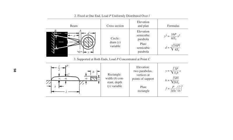
B A
P
C
x
x
l
l
y
y
d
y3 = x2
x
d
b
y
hhy
16PπlSs
Rectangle:width (b) con-
stant, depth(y) variable
Elevation:two parabolas,
vertices atpoints of support
Plan:semicubicparabola
Plan:rectangle
d =16PlπSs
3
y =3PSsb
h =3Pl2bSs
d 3
l2
Beam
2. Fixed at One End, Load P Uniformly Distributed Over l
3. Supported at Both Ends, Load P Concentrated at Point C
Cross section
Circle:diam (y)variable
FormulasElevationand plan
Elevationsemicubicparabola
f = P2Eb
lh
3
58

FIGURE 2.17 (Continued)
P
C
C
A B
bP
x x
P
b
y = x
x
b
y
xy
3PSsh
2
Rectangle:width (y) vari-
able, depth(h) constant
Rectangle:width (b) con-
stant, depth(y or y1)variable
Elevation:two parabolas,
vertices atpoints of support
Plan:two triangles,
vertices atpoints of support
Plan:rectangle
b = 3Pl2Ssh
2
y2 =6P(l – p)
blSs
6P(l – p)pblSs
x1y12 =
6PpblSs
f = 3Pl3
8Ebh3
h =
h
hh
l – p
yy y 1
l2
Elevation:rectangle
h 2h 2
59

O C
P
xA B
bRectangle:
width (b) con-stant, depth(y) variable Plan:
rectangle
3Pl4bSs
h =
f =
y yh h
l2
Elevation:ellipse
Deflection at O:l2
h 2
= 1+y2
3Pl4bSs
x2
164
= 316
PbE
l2
2
lh
3
4. Supported at Both Ends, Load P Uniformly Distributed Over l
Pl3
EI
O xA B
b
Rectangle:width (b) con-
stant, depth(y) variable
Major axis = lMinor axis = 2h
Plan:rectangle
3Pl2bSs
h =
y yh h
l2
Elevation:ellipse
l2
h 2
= 1+ y2
3Pl2bSs
x2
l2
2
Beam
3. Supported at Both Ends, Load P Moving Across Span
Cross section FormulasElevationand plan
60

FIGURE 2.17 (Continued)
x
Rectangle:width (y)
variable, depth(h) constant
Plan:two parabolas
with vertices atcenter of span
y =
y b
y
b
h
l2
Elevation:rectangle
x –3PSsh
2
b = 3Pl4Ssh
2
x2
l
Beam Cross section FormulasElevationand plan
4. Supported at Both Ends, Load P Uniformly Distributed Over l
61

TABLE 2.2 Approximate Safe Loads in Pounds (kgf) on Steel Beams* (Percoyd Iron Works)(Beams supported at both ends; allowable fiber stress for steel, 16,000 lb/in2 (1.127 kgf/cm2) (basis of table) for iron, reduce values given in tableby one-eighth)
Greatest safe load, lb† Deflection, in†
Shape of section Load in middle Load distributed Load in middle Load distributed
Solid rectangle
Hollow rectangle
Solid cylinder
Hollow cylinder
Even-legged angle or tee
Channel or Z-bar
Deck beam
I-beam
*L � distance between supports, ft (m); A � sectional area of beam, in2 (cm2); D � depth of beam, in (cm); a � interior area, in2 (cm2);d � interior depth, in (cm); w � total working load, net tons (kgf).
† See Table 2.3 for coefficients for correcting values for various methods of support and loading.
wL3
93AD2
wL3
58AD2
3,390AD
L
1,795AD
L
wL3
80AD2
wL3
50AD2
2,760AD
L
1,380AD
L
wL3
85AD2
wL3
53AD2
3,050AD
L
1,525AD
L
wL3
52AD2
wL3
32AD2
1.770AD
L
885AD
L
wL3
38(AD2 � ad 2)
wL3
24(AD2 � ad 2)
1,333(AD � ad)
L
667(AD � ad)
L
wL3
38AD2
wL3
24AD2
1,333AD
L
667AD
L
wL3
52(AD2 � ad 2)
wL3
32(AD2 � ad 2)
1,780(AD � ad)
L
890(AD � ad)
L
wL3
52AD2
wL3
32AD2
1,780AD
L
890AD
L
62

TABLE 2.3 Coefficients for Correcting Values in Table 2.2 for Various Methods of Support and of Loading*
Max relativedeflection under
Max relative max relative safeConditions of loading safe load load
Beam supported at endsLoad uniformly distributed over span 1.0 1.0Load concentrated at center of span 0.80Two equal loads symmetrically concentrated l/4cLoad increasing uniformly to one end 0.974 0.976Load increasing uniformly to center 0.96Load decreasing uniformly to center 1.08
Beam fixed at one end, cantileverLoad uniformly distributed over span 2.40Load concentrated at end 3.20Load increasing uniformly to fixed end 1.92
Beam continuous over two supports equidistant from endsLoad uniformly distributed over span
1. If distance a 0.2071l l2/4a2
2. If distance a � 0.2071l l/(l – 4a)3. If distance a � 0.2071l 5.83
Two equal loads concentrated at ends l/4a
*l � length of beam; c � distance from support to nearest concentrated load; a � distance from support to end of beam.
3�8
1�8
1�4
3�2
3�4
1�2
63

64 CHAPTER TWO
Figure 2.19 shows the condition when two equal loads are equally distant onopposite sides of the center of the beam. The moment is then equal under thetwo loads.
If two moving loads are of unequal weight, the condition for maximummoment is the maximum moment occurring under the heavier wheel when thecenter of the beam bisects the distance between the resultant of the loads andthe heavier wheel. Figure 2.20 shows this position and the shear and momentdiagrams.
FIGURE 2.18 Two equal concentrated movingloads.
l2
PP
R1 R2la
x
1
Moment
Shear
M1M2
2
FIGURE 2.19 Two equal moving loads equallydistant on opposite sides of the center.
PP
R1 R2 = P= P
l2
a2
l2
Moment
Shear
a2

BEAM FORMULAS 65
FIGURE 2.20 Two moving loads of unequal weight.
P2P
R1 R2
l2a
6
a
Moment
Shear
l2
When several wheel loads constituting a system are on a beam or beams, theseveral wheels must be examined in turn to determine which causes the greatestmoment. The position for the greatest moment that can occur under a givenwheel is, as stated earlier, when the center of the span bisects the distancebetween the wheel in question and the resultant of all loads then on the span.The position for maximum shear at the support is when one wheel is passing offthe span.
CURVED BEAMS
The application of the flexure formula for a straight beam to the case of acurved beam results in error. When all “fibers” of a member have the samecenter of curvature, the concentric or common type of curved beam exists(Fig. 2.21). Such a beam is defined by the Winkler-Bach theory. The stress ata point y units from the centroidal axis is
(2.18)
M is the bending moment, positive when it increases curvature; y is posi-tive when measured toward the convex side; A is the cross-sectional area;
S �M
AR �1 �y
Z (R � y) �

66 CHAPTER TWO
R is the radius of the centroidal axis; Z is a cross-section property definedby
(2.19)
Analytical expressions for Z of certain sections are given in Table 2.4. Z canalso be found by graphical integration methods (see any advanced strengthbook). The neutral surface shifts toward the center of curvature, or inside fiber,an amount equal to e � ZR/(Z � 1). The Winkler-Bach theory, though practi-cally satisfactory, disregards radial stresses as well as lateral deformations andassumes pure bending. The maximum stress occurring on the inside fiber isS � Mhi/AeRi, whereas that on the outside fiber is S � Mho/AeRo.
The deflection in curved beams can be computed by means of the moment-area theory.
The resultant deflection is then equal to in the direction defined by Deflections can also be found conveniently by useof Castigliano’s theorem. It states that in an elastic system the displacement inthe direction of a force (or couple) and due to that force (or couple) is the partialderivative of the strain energy with respect to the force (or couple).
A quadrant of radius R is fixed at one end as shown in Fig. 2.22. The force Fis applied in the radial direction at free-end B. Then, the deflection of B isBy moment area,
y � R sin � x � R(1 � cos �) (2.20)
ds � Rd� M � FR sin � (2.21)
(2.22)B�x � FR3
4EI B�y � �
FR3
2EI
tan � � �y / �x.�0 � ��2
x � �2y
Z � �1
A� y
R � ydA
F
ho
a
F
e
hi
RiR
FRo
+y
Neutralsurface
F
FIGURE 2.21 Curved beam.

TABLE 2.4 Analytical Expressions for Z
Section Expression
A � 2 [(t � b)C1 � bC2]
Z � �1 �R
A �b ln � R � C2
R � C2� � (t � b) ln � R � C1
R � C1� �
and A � tC1 � (b � t) C3 � bC2
Z � �1 �R
A �t ln (R � C1) � (b � t) ln (R � C0) � b ln (R � C2) �
Z � �1 � 2 � R
r � � R
r� B�
R
r �2
� 1 �
Z � �1 �R
h �lnR � C
R � C �h
R
Section
C
r
R
b
b
C1
C1
C3 C2R
C2 R
t
t
r
67

68 CHAPTER TWO
and (2.23)
at (2.24)
By Castigliano,
(2.25)
Eccentrically Curved Beams
These beams (Fig. 2.23) are bounded by arcs having different centers of cur-vature. In addition, it is possible for either radius to be the larger one. Theone in which the section depth shortens as the central section is approachedmay be called the arch beam. When the central section is the largest, thebeam is of the crescent type.
Crescent I denotes the beam of larger outside radius and crescent II oflarger inside radius. The stress at the central section of such beams may befound from S � KMC/I. In the case of rectangular cross section, the equationbecomes S � 6KM/bh2, where M is the bending moment, b is the width of thebeam section, and h its height. The stress factors, K for the inner boundary,established from photoelastic data, are given in Table 2.5. The outside radiusis denoted by Ro and the inside by Ri. The geometry of crescent beams is suchthat the stress can be larger in off-center sections. The stress at the central
B�x � FR3
4EI B�y � �
FR3
2EI
� 32.5�
� tan�1 2
�x � tan�1 ��FR3
2EI�
4EI
FR3 ��B �
FR3
2EI B1 � 2
4
FIGURE 2.22 Quadrant with fixedend.
y
BF X
A
R
θ
FIGURE 2.23 Eccentrically curved beams.
Ro
Ri
Ri
Ro
Ro
RiRi
Ro

BEAM FORMULAS 69
TABLE 2.5 Stress Factors for Inner Boundary at Central Section (see Fig. 2.23)
1. For the arch-type beams
(a)
(b)
(c) In the case of larger section ratios use the equivalent beam solution
2. For the crescent I-type beams
(a)
(b)
(c)
3. For the crescent II-type beams
(a)
(b)
(c) K � 1.081 � h
Ro � Ri�
0.0270 if Ro � Ri
h 20
K � 1.119 � h
Ro � Ri�
0.0378 if 8 �Ro � Ri
h� 20
K � 0.897 � 1.098h
Ro � Ri
if Ro � Ri
h� 8
K � 1.092 � h
Ro � Ri�
0.0298 if Ro � Ri
h 20
K � 0.959 � 0.769h
Ro � Ri
if 2 �Ro � Ri
h� 20
K � 0.570 � 1.536h
Ro � Ri
if Ro � Ri
h� 2
K � 0.899 � 1.181h
Ro � Ri
if 5 �Ro � Ri
h� 10
K � 0.834 � 1.504h
Ro � Ri
if Ro � Ri
h� 5
section determined above must then be multiplied by the position factor k,given in Table 2.6. As in the concentric beam, the neutral surface shiftsslightly toward the inner boundary. (See Vidosic, “Curved Beams with Eccen-tric Boundaries,” Transactions of the ASME, 79, pp. 1317–1321.)
ELASTIC LATERAL BUCKLING OF BEAMS
When lateral buckling of a beam occurs, the beam undergoes a combination oftwist and out-of-plane bending (Fig. 2.24). For a simply supported beam ofrectangular cross section subjected to uniform bending, buckling occurs at thecritical bending moment, given by
(2.26)Mcr �
L 2EIyGJ

70 CHAPTER TWO
TABLE 2.6 Crescent-Beam Position Stress Factors (see Fig. 2.23)*
Angle �,k
degree Inner Outer
10 1 � 0.055 H/h 1 � 0.03 H/h20 1 � 0.164 H/h 1 � 0.10 H/h30 1 � 0.365 H/h 1 � 0.25 H/h40 1 � 0.567 H/h 1 � 0.467 H/h
50 1 � 0.733 H/h
60 1 � 1.123 H/h
70 1 � 1.70 H/h
80 1 � 2.383 H/h
90 1 � 3.933 H/h
*Note: All formulas are valid for 0 � H/h � 0.325. Formulas for the inner boundary,except for 40 degrees, may be used to H/h � 0.36. H � distance between centers.
2.531 �(0.2939 � 0.7084 H/h)1/2
0.3542
2.070 �(0.4817 � 1.298 H/h)1/2
0.6492
1.756 �(0.2416 � 0.6506 H/h)1/2
0.6506
1.521 �(0.5171 � 1.382 H/h)1/2
1.382
FIGURE 2.24 (a) Simple beam subjected to equal end moments. (b)Elastic lateral buckling of the beam.
MCompressive stress
Tensile stress
L(a)
β
Mcr
Mcr
(b)
M

BEAM FORMULAS 71
where L � unbraced length of the memberE � modulus of elasticityIy � moment of inertial about minor axisG � shear modulus of elasticityJ � torsional constant
The critical moment is proportional to both the lateral bending stiffness EIy /Land the torsional stiffness of the member GJ/L.
For the case of an open section, such as a wide-flange or I-beam section,warping rigidity can provide additional torsional stiffness. Buckling of a simplysupported beam of open cross section subjected to uniform bending occurs at thecritical bending moment, given by
(2.27)
where Cw is the warping constant, a function of cross-sectional shape anddimensions (Fig. 2.25).
In the preceding equations, the distribution of bending moment is assumed tobe uniform. For the case of a nonuniform bending-moment gradient, bucklingoften occurs at a larger critical moment. Approximation of this critical bending
Mcr �
L BEIy �GJ � ECw
2
L2 �
FIGURE 2.25 Torsion-bending constants for torsional buckling. A � cross-sectionalarea; Ix � moment of inertia about x–x axis; Iy � moment of inertia about y–y axis. (AfterMcGraw-Hill, New York). Bleich, F., Buckling Strength of Metal Structures.
Area A
y
y
x–
–
xxh
144
(a) Equal-leg angle (b) Un-equal-leg angle (c) T Section
b2
bt
tt
h
b3t3
t
b
w
Cw =A3
Cw =
4Iy + x2 A
(d) Channel (e) Symmetrical I
h2Cw = I – 4
h2IyCw =4Ix
h2A
36 144h3w3
36+(b1
3 + b23)t3Cw =
y
y
xxh

72 CHAPTER TWO
moment, Mcr� may be obtained by multiplying Mcr given by the previous equa-tions by an amplification factor
(2.28)
where (2.29)
and Mmax � absolute value of maximum moment in the unbraced beam segmentMA � absolute value of moment at quarter point of the unbraced beam
segmentMB � absolute value of moment at centerline of the unbraced beam segmentMC � absolute value of moment at three-quarter point of the unbraced
beam segment
Cb equals 1.0 for unbraced cantilevers and for members where the momentwithin a significant portion of the unbraced segment is greater than, or equal to,the larger of the segment end moments.
COMBINED AXIAL AND BENDING LOADS
For short beams, subjected to both transverse and axial loads, the stresses aregiven by the principle of superposition if the deflection due to bending may beneglected without serious error. That is, the total stress is given with sufficientaccuracy at any section by the sum of the axial stress and the bending stresses.The maximum stress, lb/in2 (MPa), equals
(2.30)
where P � axial load, lb (N )A � cross-sectional area, in2 (mm2)M � maximum bending moment, in lb (Nm)c � distance from neutral axis to outermost fiber at the section where max-
imum moment occurs, in (mm)I � moment of inertia about neutral axis at that section, in4 (mm4)
When the deflection due to bending is large and the axial load producesbending stresses that cannot be neglected, the maximum stress is given by
(2.31)
where d is the deflection of the beam. For axial compression, the moment Pdshould be given the same sign as M; and for tension, the opposite sign, but the
f �P
A� (M � Pd)
c
I
f �P
A�
Mc
I
Cb �12.5Mmax
2.5Mmax � 3MA � 4MB � 3MC
M �cr � Cb Mcr

BEAM FORMULAS 73
minimum value of M � Pd is zero. The deflection d for axial compression andbending can be closely approximated by
(2.32)
where d0 � deflection for the transverse loading alone, in (mm); and Pc � criti-cal buckling load 2EI / L2, lb (N).
UNSYMMETRICAL BENDING
When a beam is subjected to loads that do not lie in a plane containing a princi-pal axis of each cross section, unsymmetrical bending occurs. Assuming thatthe bending axis of the beam lies in the plane of the loads, to preclude torsion,and that the loads are perpendicular to the bending axis, to preclude axial com-ponents, the stress, lb/in2 (MPa), at any point in a cross section is
(2.33)
where Mx � bending moment about principal axis XX,in lb (Nm)
My � bending moment about principal axis YY,in lb (Nm)
x � distance from point where stress is to be computed to YY axis,in (mm)
y � distance from point to XX axis, in (mm)Ix � moment of inertia of cross section about XX, in (mm4)Iy � moment of inertia about YY, in (mm4)
If the plane of the loads makes an angle � with a principal plane, the neutralsurface forms an angle � with the other principal plane such that
(2.34)
ECCENTRIC LOADING
If an eccentric longitudinal load is applied to a bar in the plane of symmetry, itproduces a bending moment Pe, where e is the distance, in (mm), of the load Pfrom the centroidal axis. The total unit stress is the sum of this moment and thestress due to P applied as an axial load:
(2.35)f �P
A�
Pec
I�
P
A �1 �ec
r 2 �
tan � �Ix
Iy
tan �
f �Mx y
Ix
�My x
Iy
d �d0
1 � (P/Pc)

74 CHAPTER TWO
where A � cross-sectional area, in2 (mm2)c � distance from neutral axis to outermost fiber, in (mm)I � moment of inertia of cross section about neutral axis, in4 (mm4)r � radius of gyration � , in (mm)
Figure 2.1 gives values of the radius of gyration for several cross sections.If there is to be no tension on the cross section under a compressive load, e
should not exceed r2/c. For a rectangular section with width b, and depth d, theeccentricity, therefore, should be less than b/6 and d/6 (i.e., the load should notbe applied outside the middle third). For a circular cross section with diameter D,the eccentricity should not exceed D/8.
When the eccentric longitudinal load produces a deflection too large to beneglected in computing the bending stress, account must be taken of the addi-tional bending moment Pd, where d is the deflection, in (mm). This deflectionmay be closely approximated by
(2.36)
Pc is the critical buckling load 2EI/L2, lb (N).If the load P, does not lie in a plane containing an axis of symmetry, it pro-
duces bending about the two principal axes through the centroid of the section.The stresses, lb/in2 (MPa), are given by
(2.37)
where A � cross-sectional area, in2 (mm2)ex � eccentricity with respect to principal axis YY, in (mm)ey � eccentricity with respect to principal axis XX, in (mm)cx � distance from YY to outermost fiber, in (mm)cy � distance from XX to outermost fiber, in (mm)Ix � moment of inertia about XX, in4 (mm4)Iy � moment of inertia about YY, in4 (mm4)
The principal axes are the two perpendicular axes through the centroid forwhich the moments of inertia are a maximum or a minimum and for which theproducts of inertia are zero.
NATURAL CIRCULAR FREQUENCIES AND NATURALPERIODS OF VIBRATION OF PRISMATIC BEAMS
Figure 2.26 shows the characteristic shape and gives constants for determi-nation of natural circular frequency � and natural period T, for the firstfour modes of cantilever, simply supported, fixed-end, and fixed-hingedbeams. To obtain �, select the appropriate constant from Fig. 2.26 and
f �P
A�
Pexcx
Iy
�Peycy
Ix
d �4eP/Pc
(1 � P/Pc)
2I/A

Type of Support Fundamental Mode
L
Second Mode Third Mode Fourth Mode
Cantilever
20.0 125 350
0.315
56.0
Fixed
Fixed-hinged
0.112224
0.0281502
0.0125
0.774L
0.5L 0.356L
0.644L684
0.132L
0.0503 0.0180 0.0092
0.5L
0.359L 0.359L 0.278L
0.278L1,1330.0056
LLSimple
wL4/EI =EI/wL4 =
wL4/EIω
ω
ω
=EI/wL4T
T
T
ωT
=
wL4/EI =EI/wL4 =
wL4/EI =EI/wL4 =
3L3
LL
L
2L2
L4
L4
L2897
0.0070
1270.0496
3500.0180
0.56L 0.384L 0.308L 0.294L
0.529L1,1110.0062
5910.0106
2830.0222
87.20.0722
0.235L
6840.0092
0.094L
FIGURE 2.26 Coefficients for computing natural circular frequencies and natural periods of vibrationof prismatic beams.
75

76 CHAPTER TWO
multiply it by . To get T, divide the appropriate constant by .In these equations,
� � natural frequency, rad/sW � beam weight, lb per linear ft (kg per linear m)L � beam length, ft (m)E � modulus of elasticity, lb/in2 (MPa)I � moment of inertia of beam cross section, in4 (mm4)T � natural period, s
To determine the characteristic shapes and natural periods for beams withvariable cross section and mass, use the Rayleigh method. Convert the beaminto a lumped-mass system by dividing the span into elements and assumingthe mass of each element to be concentrated at its center. Also, compute all quanti-ties, such as deflection and bending moment, at the center of each element. Startwith an assumed characteristic shape.
TORSION IN STRUCTURAL MEMBERS
Torsion in structural members occurs when forces or moments twist the beamor column. For circular members, Hooke’s law gives the shear stress at any giv-en radius, r. Table 2.7 shows the polar moment of inertia, J, and the maximumshear for five different structural sections.
STRAIN ENERGY IN STRUCTURAL MEMBERS*
Strain energy is generated in structural members when they are acted on byforces, moments, or deformations. Formulas for strain energy, U, for shear,torsion and bending in beams, columns, and other structural members are:
Strain Energy in Shear.
For a member subjected to pure shear, strain energy is given by
(2.38)
(2.39)
where V � shear load� � shear deformationL � length over which the deformation takes placeA � shear areaG � shear modulus of elasticity
U �AG� 2
2L
U �V 2L
2AG
�EI/wL4�EI/wL4
*Brockenbrough and Merritt—Structural Steel Designer’s Handbook, McGraw-Hill.

TABLE 2.7 Polar Moment of Intertia and Maximum Torsional Shear
BEAM FORMULAS 77
Strain Energy in Torsion
For a member subjected to torsion
(2.40)
(2.41)U �JG� 2
2L
U �T 2L
2JG
2r
2R2r
a
a
b
a
Polar moment ofinertia J
Maximum shear*vmax
at periphery
2Tπr3
at midpointof each side
at midpointof longer sides
– 0.21 1 –
R = 2T208a3
T(3a – 1.8b)a2b2
π(R4 – r4)
at outerperiphery
2TRπ(R4 – r4)
b4
12a4
at midpointof each side
20Ta3
12
πr4
12
0.0214a4
13
ba
0.141a4
ab3
*T � twisting moment, or torque.

78 CHAPTER TWO
Pab2
L2a
P
P
wk/twk/t
wk/t
wk/t
aL
aL
wk/t
P P P P P P
L–2a
L/4 L/4 L/4 L/5 L/5 L/5
L/3
P
P
P
L/3
L/2 L/2
L/3
L/5 L/5L/4
L/2
a a
P
P
b
Pa2bL2
PL8
PL8
2PL9
2PL5
wL2
12
5wL2
19211wL2
192
wk/t
wk/t
wk/t
L/2
L/2
L/2 L/2
L/2
L/2
L/2 L/2
L/4 L/4
L/2
3wL2
160wL2
30
7wL2
960
wk/t
wk/t wk/t
5wL2
96
wL2
32
5wL2
192
23wL2
960
wL2
30wL2
20
wa2(6 – 8a + 3a2)L2
12wa3(4 – 3a)L2
12
wa2(10 – 15a + 6a2)L2
30wa3(5 – 4a)L2
20
wL2
15
wL2
60
wk/t
wk/t
wk/t
wk/t wk/t
aL
aL
aL
aL
M
wa2(10 – 10a + 3a2)L2
60
Parabola
Parabola
wa3(5 – 3a)L2
60
wa2(3 – 2a)L2
6
M4
MM4
Ma(1 – 3a)M(1 – a) (3a – 1)
Pa(L – a)L
5PL16
–
FIGURE 2.27 Fixed-end moments in beams. (Brockenbrongh and Merritt-StructuralDesigner’s Handbook, McGraw-Hill.)

BEAM FORMULAS 79
where T � torque� � angle of twistL � length over which the deformation takes placeJ � polar moment of inertia
G � shear modulus of elasticity
Strain Energy in Bending
For a member subjected to pure bending (constant moment)
(2.42)
(2.43)
where M � bending moment� � angle through which one end of beam rotates with respect to the
other endL � length over which the deformation takes placeI � moment of inertia
E � modulus of elasticity
For beams carrying transverse loads, the total strain energy is the sum of theenergy for bending and that for shear.
FIXED-END MOMENTS IN BEAMS
Figure 2.27 gives formulas for fixed-end moments in a variety of beams. Theformat of this illustration gives easy access to these useful formulas.
U �EI� 2
2L
U �M 2L
2EI

This page intentionally left blank

CHAPTER 3 COLUMN
FORMULAS
GENERAL CONSIDERATIONS
Columns are structural members subjected to direct compression. All columnscan be grouped into the following three classes:
1. Compression blocks are so short (with a slenderness ratio—that is, unsup-ported length divided by the least radius of gyration of the member—below 30)that bending is not potentially occurring.
2. Columns so slender that bending under load is given are termed long columnsand are defined by Euler’s theory.
3. Intermediate-length columns, often used in structural practice, are calledshort columns.
Long and short columns usually fail by buckling when their critical load isreached. Long columns are analyzed using Euler’s column formula, namely,
(3.1)
In this formula, the coefficient n accounts for end conditions. When the columnis pivoted at both ends, n � 1; when one end is fixed and the other end isrounded, n � 2; when both ends are fixed, n � 4; and when one end is fixedand the other is free, n � 0.25. The slenderness ratio separating long columnsfrom short columns depends on the modulus of elasticity and the yield strengthof the column material. When Euler’s formula results in (Pcr /A) > Sy, strengthinstead of buckling causes failure, and the column ceases to be long. In quickestimating numbers, this critical slenderness ratio falls between 120 and 150.Table 3.1 gives additional column data based on Euler’s formula.
SHORT COLUMNS
Stress in short columns can be considered to be partly due to compression andpartly due to bending. Empirical, rational expressions for column stress are, in
Pcr �n 2EI
l2 �n 2EA
(l/r)2
81

TABLE 3.1 Strength of Round-Ended Columns According to Euler’s Formula*
Low- Medium-Wrought carbon carbon
Material† Cast iron iron steel steel
Ultimate compressive strength, lb/in2 107,000 53,400 62,600 89,000Allowable compressive stress, lb/in2 7,100 15,400 17,000 20,000
(maximum)Modulus of elasticity 14,200,000 28,400,000 30,600,000 31,300,000Factor of safety 8 5 5 5Smallest I allowable at worst section, in4 Pl 2 Pl 2 Pl 2 Pl 2
17,500,000 56,000,000 60,300,000 61,700,000Limit of ratio, l/r 50.0 60.6 59.4 55.6
Rectangle 14.4 17.5 17.2 16.0
Circle 12.5 15.2 14.9 13.9Circular ring of small thickness 17.6 21.4 21.1 19.7
*P � allowable load, lb; l � length of column, in; b � smallest dimension of a rectangular section, in; d � diameter of a circular sec-tion, in; r � least radius of gyration of section.
†To convert to SI units, use: 1b/in2 � 6.894 � kPa; in4 � (25.4)4 � mm4.
�r � d w1�8�, l/d
�r � 1�4 d�, l/d
�r � bw1�12�, l/b
82

COLUMN FORMULAS 83
Short
S
Com
pres
sion
blo
cks
Long
Euler column
Critical L/r
Parabolic type
Straight linetype
L/r
FIGURE 3.1 L /r plot for columns.
general, based on the assumption that the permissible stress must be reducedbelow that which could be permitted were it due to compression only. The mannerin which this reduction is made determines the type of equation and the slender-ness ratio beyond which the equation does not apply. Figure 3.1 shows the curvesfor this situation. Typical column formulas are given in Table 3.2.
ECCENTRIC LOADS ON COLUMNS
When short blocks are loaded eccentrically in compression or in tension, that is,not through the center of gravity (cg), a combination of axial and bending stressresults. The maximum unit stress SM is the algebraic sum of these two unit stresses.
In Fig. 3.2, a load, P, acts in a line of symmetry at the distance e from cg; r �radius of gyration. The unit stresses are (1) Sc, due to P, as if it acted through cg,and (2) Sb, due to the bending moment of P acting with a leverage of e about cg.Thus, unit stress, S, at any point y is
(3.2)
y is positive for points on the same side of cg as P, and negative on the oppositeside. For a rectangular cross section of width b, the maximum stress, SM �Sc(1 � 6e/b). When P is outside the middle third of width b and is a compres-sive load, tensile stresses occur.
For a circular cross section of diameter d, SM � Sc(1 � 8e/d). The stress due tothe weight of the solid modifies these relations.
Note that in these formulas e is measured from the gravity axis and givestension when e is greater than one-sixth the width (measured in the same directionas e), for rectangular sections, and when greater than one-eighth the diameter,for solid circular sections.
� Sc(1 � ey/r 2)
� (P/A) � Pey/I
S � Sc � Sb

84 CHAPTER THREE
If, as in certain classes of masonry construction, the material cannot withstandtensile stress and, thus, no tension can occur, the center of moments (Fig. 3.3) istaken at the center of stress. For a rectangular section, P acts at distance k from thenearest edge. Length under compression � 3k, and SM � 2/3 P/hk. For a circular
section, SM � [0.372 � 0.056 (k /r)]P/k , where r � radius and k � distanceof P from circumference. For a circular ring, S � average compressive stress oncross section produced by P; e � eccentricity of P; z � length of diameter undercompression (Fig. 3.4). Values of z /r and of the ratio of Smax to average S are givenin Tables 3.3 and 3.4.
�rk
TABLE 3.2 Typical Short-Column Formulas
Formula Material Code Slenderness ratio
Carbon steels AISC
Carbon steels Chicago
Carbon steels AREA
Carbon steels Am. Br. Co.
Alloy-steel ANCtubing
Cast iron NYC
2017ST ANCaluminum
Spruce ANC
Steels Johnson
Steels Secant
*Scr � theoretical maximum; c � end fixity coefficient; c � 2, both ends pivoted; c � 2.86, onepivoted, other fixed; c � 4, both ends fixed; c � 1 one fixed, one free.
†Is initial eccentricity at which load is applied to center of column cross section.
l
r� critical†Scr �
Sy
1 �ec
r2 sec � l
r BP
4AE �
l
r� B
2n 2E
Sy
*Scr � Sy �1 �Sy
4n 2E � l
r �2
�
1
wcr� 72*Scr � 5,000 �
0.5
c � l
r �2
1
wcr� 94*Scr � 34,500 �
245
wc� l
r �
l
r� 70Sw � 9,000 � 40 � l
r �
l
wcr� 65*Scr � 135,000 �
15.9
c � l
r �2
60 �l
r� 120Sw � 19,000 � 100 � l
r �
l
r� 150Sw � 15,000 � 50 � l
r �
l
r� 120Sw � 16,000 � 70 � l
r �
l
r� 120Sw � 17,000 � 0.485 � l
r �2

COLUMN FORMULAS 85
P
Pk
e
e
b
PA
PeyI
PeyI
PeyI Pey
I
PA
PA
FIGURE 3.2 Load plot for columns.
FIGURE 3.3 Load plot for columns.
Smax
r1r
S A
e
Z
Z
Smax
FIGURE 3.4 Circular columnload plot.
Pk
e
b
c. of g.O
SM3k
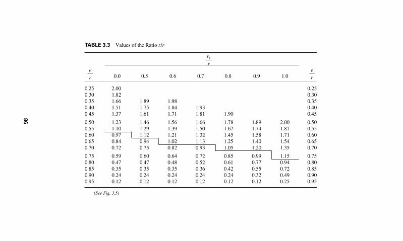
TABLE 3.3 Values of the Ratio z/r
0.0 0.5 0.6 0.7 0.8 0.9 1.0
0.25 2.00 0.250.30 1.82 0.300.35 1.66 1.89 1.98 0.350.40 1.51 1.75 1.84 1.93 0.400.45 1.37 1.61 1.71 1.81 1.90 0.45
0.50 1.23 1.46 1.56 1.66 1.78 1.89 2.00 0.500.55 1.10 1.29 1.39 1.50 1.62 1.74 1.87 0.550.60 0.97 1.12 1.21 1.32 1.45 1.58 1.71 0.600.65 0.84 0.94 1.02 1.13 1.25 1.40 1.54 0.650.70 0.72 0.75 0.82 0.93 1.05 1.20 1.35 0.70
0.75 0.59 0.60 0.64 0.72 0.85 0.99 1.15 0.750.80 0.47 0.47 0.48 0.52 0.61 0.77 0.94 0.800.85 0.35 0.35 0.35 0.36 0.42 0.55 0.72 0.850.90 0.24 0.24 0.24 0.24 0.24 0.32 0.49 0.900.95 0.12 0.12 0.12 0.12 0.12 0.12 0.25 0.95
(See Fig. 3.5)
r1
re
r
e
r
86

TABLE 3.4 Values of the Ratio Smax/Savg
0.0 0.5 0.6 0.7 0.8 0.9 1.0
0.00 1.00 1.00 1.00 1.00 1.00 1.00 1.00 0.000.05 1.20 1.16 1.15 1.13 1.12 1.11 1.10 0.050.10 1.40 1.32 1.29 1.27 1.24 1.22 1.20 0.100.15 1.60 1.48 1.44 1.40 1.37 1.33 1.30 0.150.20 1.80 1.64 1.59 1.54 1.49 1.44 1.40 0.200.25 2.00 1.80 1.73 1.67 1.61 1.55 1.50 0.250.30 2.23 1.96 1.88 1.81 1.73 1.66 1.60 0.300.35 2.48 2.12 2.04 1.94 1.85 1.77 1.70 0.350.40 2.76 2.29 2.20 2.07 1.98 1.88 1.80 0.400.45 3.11 2.51 2.39 2.23 2.10 1.99 1.90 0.45
(In determining S average, use load P divided by total area of cross section)
r1
r
e
r
e
r
87

88 CHAPTER THREE
The kern is the area around the center of gravity of a cross section withinwhich any load applied produces stress of only one sign throughout the entirecross section. Outside the kern, a load produces stresses of different sign.Figure 3.5 shows kerns (shaded) for various sections.
For a circular ring, the radius of the kern r � D[1�(d/D)2]/8.For a hollow square (H and h � lengths of outer and inner sides), the kern is
a square similar to Fig. 3.5(a), where
(3.3)
For a hollow octagon, Ra and Ri are the radii of circles circumscribing the outerand inner sides respectively; thickness of wall � 0.9239(Ra – Ri); and the kern is anoctagon similar to Fig. 3.5(c), where 0.2256R becomes 0.2256Ra[1 � (Ri/Ra)2].
COLUMNS OF SPECIAL MATERIALS*
Here are formulas for columns made of special materials. The nomenclature forthese formulas is:
rmin �H
6
1
�2 �1 � � h
H �2 � � 0.1179H �1 � � h
H �2 �
h
4
bb
3 h1
(f)(e)
(b)
R R.226R
(a)
2rmin.
(c)
d
D
2r
r2
r1
3b
3b
b3
hb
3h
h
6h
6h
3h
3h
h
4d
d
(d)
4h1 3 h2
FIGURE 3.5 Column characteristics.
*Roark—Formulas for Stress and Strain, McGraw-Hill.

COLUMN FORMULAS 89
Nomenclature for formulas Eqs. (3.4) through (3.12):
Q � allowable load, lb
P � ultimate load, lb
A � section area of column, sq in
L � length of column, in
r � least radium of gyration of column section, in
Su � ultimate strength, psi
Sy � yield point or yield strength of material, psi
E � modulus of elasticity of material, psi
m � factor of safety
(L/r) � critical slenderness ratio
For columns of cast iron that are hollow, round, with flat ends, used inbuildings:
(3.4)
(3.5)
(3.6)
(3.7)
Min diameter � 6 in; min thickness � 1/2 in
(3.8)
For structural aluminum columns with the following specifications:
used in nonwelded building structures in structural shapes or in fabricated formwith partial constraint:
(3.9)
(3.10)L
r 10 � 67
Q
A� 20,400 � 135
L
r
L
r� 10
Q
A� 19,000
6061 � T6 6062 � T6
sy � 35,000
su � 38,000
E � 10,000,000
P
A� 34,000 � 88
L
r
MaxL
r� 70
Q
A� 9000 � 40
L
r
MaxQ
A� 10,000; max
L
r� 100
Q
A� 12,000 � 60
L
r

90 CHAPTER THREE
(3.11)
(3.12)
COLUMN BASE PLATE DESIGN
Base plates are usually used to distribute column loads over a large enough areaof supporting concrete construction that the design bearing strength of the con-crete is not exceeded. The factored load, Pu, is considered to be uniformly dis-tributed under a base plate.
The nominal bearing strength, fp, kip/in2 or ksi (MPa) of the concrete isgiven by
(3.13)
where fc� � specified compressive strength of concrete, ksi (MPa)A1 � area of the base plate, in2 (mm2)A2 � area of the supporting concrete that is geometrically similar to and
concentric with the loaded area, in2 (mm2)
In most cases, the bearing strength, fp is , when the concrete support isslightly larger than the base plate or , when the support is a spread footing,pile cap, or mat foundation. Therefore, the required area of a base plate for afactored load Pu is
(3.14)
where �c is the strength reduction factor � 0.6. For a wide-flange column, A1
should not be less than bf d, where bf is the flange width, in (mm), and d is thedepth of column, in (mm).
The length N, in (mm), of a rectangular base plate for a wide-flange columnmay be taken in the direction of d as
(3.15)
The width B, in (mm), parallel to the flanges, then, is
(3.16)B �A1
N
N �2A1 � � d or � � 0.5(0.95d � 0.80bf)
A1 �Pu
�c0.85 fc�
1.7f �c
0.85f �c
fp � 0.85f c�BA1
A1 and B
A2
A1� 2
P
A� 1.95
Q
A
L
r 67
Q
A�
51,000,000
(L/r)2

COLUMN FORMULAS 91
The thickness of the base plate tp, in (mm), is the largest of the values givenby the equations that follow
(3.17)
(3.18)
(3.19)
where m � projection of base plate beyond the flange and parallel to the web,in (mm)
� (N � 0.95d)/2n � projection of base plate beyond the edges of the flange and perpendi-
cular to the web, in (mm)� (B � 0.80bf)/2
�
� �
X �
AMERICAN INSTITUTE OF STEEL CONSTRUCTIONALLOWABLE-STRESS DESIGN APPROACH
The lowest columns of a structure usually are supported on a concrete founda-tion. The area, in square inches (square millimeters), required is found from
(3.20)
where P is the load, kip (N) and Fp is the allowable bearing pressure on sup-port, ksi (MPa).
The allowable pressure depends on strength of concrete in the foundationand relative sizes of base plate and concrete support area. If the base plate occu-pies the full area of the support, , where is the 28-day compres-sive strength of the concrete. If the base plate covers less than the full area,
, where A1 is the base-plate area (B � N), and A2
is the full area of the concrete support.Eccentricity of loading or presence of bending moment at the column base
increases the pressure on some parts of the base plate and decreases it onother parts. To compute these effects, the base plate may be assumed com-pletely rigid so that the pressure variation on the concrete is linear.
Plate thickness may be determined by treating projections m and n of the baseplate beyond the column as cantilevers. The cantilever dimensions m and n are
FP � 0.35fc��A2/A1 � 0.70f �c
f �cFp � 0.35f �c
A �P
FP
(4 dbf)/(d � bf)2][Pu/(� � 0.85f�c �1)(22X)/[1 � 2(1 � X)] � 1.0
�(dbf)/4n�
tp � �n�B2Pu
0.9Fy BN
tp � nB2Pu
0.9Fy BN
tp � mB2Pu
0.9Fy BN

92 CHAPTER THREE
usually defined as shown in Fig. 3.6. (If the base plate is small, the area of thebase plate inside the column profile should be treated as a beam.) Yield-lineanalysis shows that an equivalent cantilever dimension can be defined as
, and the required base plate thickness tp can be calculated from
(3.21)
where l � max (m, n, ), in (mm)fp � P/(BN) � Fp, ksi (MPa)
Fy � yield strength of base plate, ksi (MPa)P � column axial load, kip (N)
For columns subjected only to direct load, the welds of column to baseplate, as shown in Fig. 3.6, are required principally for withstanding erectionstresses. For columns subjected to uplift, the welds must be proportioned toresist the forces.
COMPOSITE COLUMNS
The AISC load-and-resistance factor design (LRFD) specification for structuralsteel buildings contains provisions for design of concrete-encased compressionmembers. It sets the following requirements for qualification as a composite col-umn: The cross-sectional area of the steel core—shapes, pipe, or tubing—should
n�
tp � 2lBfp
Fy
n� � 1�42dbf
n�
(76.
2 m
m)
(76.
2 m
m)
3"3"
N
B
nn
b f
1/4
1/4
1/422
For columns10" or larger
d
m m0.95d
0.80
b f
FIGURE 3.6 Column welded to a base plate.

be at least 4 percent of the total composite area. The concrete should be rein-forced with longitudinal load-carrying bars, continuous at framed levels, andlateral ties and other longitudinal bars to restrain the concrete; all should haveat least in (38.1 mm) of clear concrete cover. The cross-sectional area oftransverse and longitudinal reinforcement should be at least 0.007 in2
(4.5 mm2) per in (mm) of bar spacing. Spacing of ties should not exceed two-thirds of the smallest dimension of the composite section. Strength of the con-crete should be between 3 and 8 ksi (20.7 and 55.2 MPa) for normal-weightconcrete and at least 4 ksi (27.6 MPa) for lightweight concrete. Specified mini-mum yield stress Fy of steel core and reinforcement should not exceed 60 ksi(414 MPa). Wall thickness of steel pipe or tubing filled with concrete shouldbe at least or , where b is the width of the face of a rectangularsection, D is the outside diameter of a circular section, and E is the elastic mod-ulus of the steel.
The AISC LRFD specification gives the design strength of an axially loadedcomposite column as �Pn, where � � 0.85 and Pn is determined from
(3.22)
For �c � 1.5
(3.23)
For �c 1.5
(3.24)
where �c �
KL � effective length of column, in (mm)As � gross area of steel core, in2 (mm2)
Fmy �
Em �
rm � radius of gyration of steel core, in � 0.3 of the overall thickness of thecomposite cross section in the plane of buckling for steel shapes
Ac � cross-sectional area of concrete, in2 (mm2)Ar � area of longitudinal reinforcement, in2 (mm2)Ec � elastic modulus of concrete, ksi (MPa)
Fyr � specified minimum yield stress of longitudinal reinforcement, ksi(MPa)
For concrete-filled pipe and tubing, c1 � 1.0, c2 � 0.85, and c3 � 0.4. Forconcrete-encased shapes, c1 � 0.7, c2 � 0.6, and c3 � 0.2.
When the steel core consists of two or more steel shapes, they should be tiedtogether with lacing, tie plates, or batten plates to prevent buckling of individ-ual shapes before the concrete attains .0.75 f �c
E � c3Ec(Ac/As)
Fy � c1Fyr(Ar /As) � c2 fc�(Ac/As)
(KL/rm )wFmy/Em
Fcr �0.877
�c2 Fmy
Fcr � 0.658l2c Fmy
�Pn � 0.85AsFcr
DwFy/8EbwFy /3E
f �c
1 1�2
COLUMN FORMULAS 93

94 CHAPTER THREE
The portion of the required strength of axially loaded encased compositecolumns resisted by concrete should be developed by direct bearing at connec-tions or shear connectors can be used to transfer into the concrete the loadapplied directly to the steel column. For direct bearing, the design strength of theconcrete is where and loaded area, in2 (mm2). Cer-tain restrictions apply.
ELASTIC FLEXURAL BUCKLING OF COLUMNS
Elastic buckling is a state of lateral instability that occurs while the material isstressed below the yield point. It is of special importance in structures with slen-der members. Euler’s formula for pin-ended columns (Fig. 3.7) gives validresults for the critical buckling load, kip (N). This formula is, with L/r as theslenderness ratio of the column,
(3.25)P � 2EA
(L/r)2
Ab ��c � 0.651.7�c fc� Ab,
P P y
y(x)P
P
P
P
L
(b)(a)
M(X)
x
M(X)
FIGURE 3.7 (a) Buckling of a pin-ended column under axial load. (b) Internal forces hold the column in equilibrium.

COLUMN FORMULAS 95
where E � modulus of elasticity of the column material, psi (Mpa)A � column cross-sectional area, in2 (mm2)r � radius of gyration of the column, in (mm)
Figure 3.8 shows some ideal end conditions for slender columns and corre-sponding critical buckling loads. Elastic critical buckling loads may be obtainedfor all cases by substituting an effective length KL for the length L of thepinned column, giving
(3.26)
In some cases of columns with open sections, such as a cruciform section,the controlling buckling mode may be one of twisting instead of lateraldeformation. If the warping rigidity of the section is negligible, torsional buck-ling in a pin-ended column occurs at an axial load of
(3.27)P �GJA
Ip
P � 2EA
(KL/r)2
Type of column Effective length Critical buckling load
L L π2EIL2
4π2EIL2
2π2EIL2
π2EI4L2
L2
~0.7L
2L
L/4
L/2
L/4
0.7L
0.3L
L
~ ~~
FIGURE 3.8 Buckling formulas for columns.

96 CHAPTER THREE
where G � shear modulus of elasticity, psi (MPa)J � torsional constantA � cross-sectional area, in2 (mm2)Ip � polar moment of inertia � Ix � Iy, in4 (mm4)
If the section possesses a significant amount of warping rigidity, the axial buck-ling load is increased to
(3.28)
where Cw is the warping constant, a function of cross-sectional shape anddimensions.
ALLOWABLE DESIGN LOADS FOR ALUMINUM COLUMNS
Euler’s equation is used for long aluminum columns, and depending on thematerial, either Johnson’s parabolic or straight-line equation is used for shortcolumns. These equations for aluminum followEuler’s equation
(3.29)
Johnson’s generalized equation
(3.30)
The value of n, which determines whether the short column formula is thestraight-line or parabolic type, is selected from Table 3.5. The transition from thelong to the short column range is given by
(3.31)
where Fe � allowable column compressive stress, psi (MPa)Fce � column yield stress and is given as a function of Fcy (compres-
sive yield stress), psi (MPa)L � length of column, ft (m)� � radius of gyration of column, in (mm)E � modulus of elasticity—noted on nomograms, psi (MPa)c � column-end fixity from Fig. 3.9
n, K, k � constants from Table 3.5
� L
� �cr � BkcE
Fce
Fc � Fce �1 � K � (L/�)
BcE
Fce
�n
�
Fe �c 2E
(L/�)2
P �A
Ip�GJ �
2ECw
L2 �
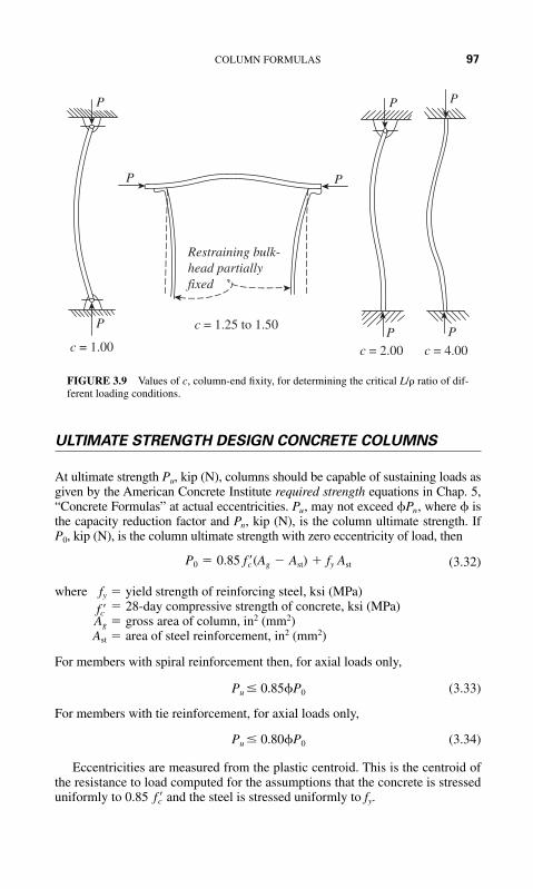
COLUMN FORMULAS 97
Restraining bulk-head partiallyfixed
P
P
P
P
P P
P P
c = 1.00
c = 1.25 to 1.50
c = 2.00 c = 4.00
FIGURE 3.9 Values of c, column-end fixity, for determining the critical L/� ratio of dif-ferent loading conditions.
ULTIMATE STRENGTH DESIGN CONCRETE COLUMNS
At ultimate strength Pu, kip (N), columns should be capable of sustaining loads asgiven by the American Concrete Institute required strength equations in Chap. 5,“Concrete Formulas” at actual eccentricities. Pu, may not exceed �Pn, where � isthe capacity reduction factor and Pn, kip (N), is the column ultimate strength. IfP0, kip (N), is the column ultimate strength with zero eccentricity of load, then
(3.32)
where fy � yield strength of reinforcing steel, ksi (MPa)fc� � 28-day compressive strength of concrete, ksi (MPa)Ag � gross area of column, in2 (mm2)Ast � area of steel reinforcement, in2 (mm2)
For members with spiral reinforcement then, for axial loads only,
(3.33)
For members with tie reinforcement, for axial loads only,
(3.34)
Eccentricities are measured from the plastic centroid. This is the centroid ofthe resistance to load computed for the assumptions that the concrete is stresseduniformly to 0.85 and the steel is stressed uniformly to fy.f �c
Pu � 0.80�P0
Pu � 0.85�P0
P0 � 0.85 f �c (Ag � Ast) � fy Ast

TABLE 3.5 Material Constants for Common Aluminum Alloys
Average ValuesFcy Fce
Type JohnsonMaterial psi MPa psi MPa K k n equation
14S–T4 34,000 234.4 39,800 274.4 0.385 3.00 1.0 Straight line24S–T3 and T4 40,000 275.8 48,000 330.9 0.385 3.00 1.0 Straight line61S–T6 35,000 241.3 41,100 283.4 0.385 3.00 1.0 Straight line14S–T6 57,000 393.0 61,300 422.7 0.250 2.00 2.0 Squared parabolic75S–T6 69,000 475.8 74,200 511.6 0.250 2.00 2.0 Squared parabolic
Ref: ANC-5.
98

COLUMN FORMULAS 99
The axial-load capacity Pu kip (N), of short, rectangular members subject toaxial load and bending may be determined from
(3.34)
(3.35)
where � eccentricity, in (mm), of axial load at end of member with respect tocentroid of tensile reinforcement, calculated by conventional methodsof frame analysis
b � width of compression face, in (mm)a � depth of equivalent rectangular compressive-stress distribution, in
(mm)As� � area of compressive reinforcement, in2 (mm2)As � area of tension reinforcement, in2 (mm2)d � distance from extreme compression surface to centroid of tensile
reinforcement, in (mm)d� � distance from extreme compression surface to centroid of compres-
sion reinforcement, in (mm)fs � tensile stress in steel, ksi (MPa)
The two preceding equations assume that a does not exceed the columndepth, that reinforcement is in one or two faces parallel to axis of bending, andthat reinforcement in any face is located at about the same distance from theaxis of bending. Whether the compression steel actually yields at ultimatestrength, as assumed in these and the following equations, can be verified bystrain compatibility calculations. That is, when the concrete crushes, the strainin the compression steel, 0.003 (c – d�)/c, must be larger than the strain whenthe steel starts to yield, fy/Es. In this case, c is the distance, in (mm), from theextreme compression surface to the neutral axis and Es is the modulus of elastic-ity of the steel, ksi (MPa).
The load, Pb for balanced conditions can be computed from the preceding Pu
equation with fs � fy and
(3.36)
The balanced moment, in. � kip (k . Nm), can be obtained from
(3.37)
� A�s fy (d � d� � d��) � As fy d���� � �0.85 fc� bab �d � d�� �
ab
2 �Mb � Pbeb
�87,000 �1d
87,000 � fy
� �1cb
a � ab
e�
Pue� � ��0.85 f �cba �d �a
2 � � As� fy (d � d� )�Pu � �(0.85 f �c ba � A�s fy � As fs)

100 CHAPTER THREE
where eb is the eccentricity, in (mm), of the axial load with respect to the plasticcentroid and is the distance, in (mm), from plastic centroid to centroid of ten-sion reinforcement.
When Pu is less than Pb or the eccentricity, e, is greater than eb, tension gov-erns. In that case, for unequal tension and compression reinforcement, the ulti-mate strength is
(3.38)
where
Special Cases of Reinforcement
For symmetrical reinforcement in two faces, the preceding Pu equation becomes
(3.39)
Column Strength When Compression Governs
For no compression reinforcement, the Pu equation becomes
(3.40)� B�1 �e�
d �2
� 2� e��m
d ��Pu � 0.85 f �cbd� ���m � 1 �
e�
d
� B�1 �e�
d �2
� 2� �m��1 �d�
d � �e�
d ��
Pu � 0.85 f �c bd� ��� � 1 �e�
d
�� � A�s /bd
� � As /bdm� � m � 1m � f �y /0.85f �c
� B�1 �e�
d �2
� 2 �(�m � ��m�)e�
d� ��m� �1 �
d�
d ���Pu � 0.85 f �c bd� ���m� � �m � �1 �
e�
d �
d��

COLUMN FORMULAS 101
When Pu is greater than Pb, or e is less than eb, compression governs. In that case,the ultimate strength is approximately
(3.41)
(3.42)
where Mu is the moment capacity under combined axial load and bending, inkip (kNm) and Po is the axial-load capacity, kip (N), of member when concen-trically loaded, as given.
For symmetrical reinforcement in single layers, the ultimate strength whencompression governs in a column with depth, h, may be computed from
(3.43)
Circular Columns
Ultimate strength of short, circular members with bars in a circle may be deter-mined from the following equations:When tension controls,
(3.44)
where D � overall diameter of section, in (mm)Ds � diameter of circle through reinforcement, in (mm)�t � Ast /Ag
When compression governs,
(3.45)
The eccentricity for the balanced condition is given approximately by
(3.46)
Short Columns
Ultimate strength of short, square members with depth, h, and with bars in acircle may be computed from the following equations:
eb � (0.24 � 0.39 �t m)D
Pu � � � Ast fv
3e/Ds � 1�
Ag f �c9.6De/(0.8D � 0.67Ds)2 � 1.18 �
Pu � 0.85 f �c D2� �B� 0.85e
D� 0.38�
2
��
1mDs
2.5D � � 0.85e
D� 0.38��
Pu � � � A�s fy
e/d � d� � 0.5�
bhf �c3he/d2 � 1.18 �
Pu �Po
1 � (Po/Pb � 1)(e/eb)
Pu � Po � (Po � Pb)Mu
Mb

102 CHAPTER THREE
When tension controls,
(3.47)
When compression governs,
(3.48)
Slender Columns
When the slenderness of a column has to be taken into account, the eccentricityshould be determined from e � Mc /Pu, where Mc is the magnified moment.
DESIGN OF AXIALLY LOADED STEEL COLUMNS*
Design of columns that are subjected to compression applied through the cen-troidal axis (axial compression) is based on the assumption of uniform stressover the gross area. This concept is applicable to both load and resistance factordesign (LRFD) and allowable stress design (ASD).
Design of an axially loaded compression member or column for both LRFDand ASD utilizes the concept of effective column length KL. The buckling coef-ficient K is the ratio of the effective column length to the unbraced length L.Values of K depend on the support conditions of the column to be designed.The AISC specifications for LRFD and ASD indicate the K should be taken asunity for columns in braced frames unless analysis indicates that a smallervalue is justified. Analysis is required for determination of K for unbracedframes, but K should not be less than unity. Design values for K recommendedby the Structural Stability Research Council for use with six idealized condi-tions of rotation and translation at column supports are illustrated in Fig. 9.1.
The axially compression strength of a column depends on its stiffness meas-ured by the slenderness ratio KL/r, where r is the radius of gyration about theplane of buckling. For serviceability considerations, AISC recommends thatKL/r not exceed 200.
LRFD strength for a compression member wf;Pn (kips) is given by
�Pn � 0.85Ag Fcr (3.49)
where � � LRFD resistance factor, less than unityPn � LFRD design strength (kips) of member (also called “maximum load”
for columns, kips):
Pu � � � Ast fy
3e/Ds � 1�
Ag f �c12he/(h � 0.67Ds)2 � 1.18 �
Pu � 0.85bhf �c� �B� e
h� 0.5�
2
� 0.67Ds
h�tm � � e
h� 0.5��
*Brockenbrough and Merritt—Structural Steel Designer’s Handbook, McGraw-Hill.

COLUMN FORMULAS 103
with � � 0.85. For �c � 1.5
Fcr � 0.658�c2 Fy (3.50)
for �c 1.5
(3.51)
where �c � (KL/r )
Fy � minimum specified yield stress of steel, ksiAg � gross area of member, in2
E � elastic modulus of the steel � 29,000 ksi
For ASD, the allowable compression stress depends on whether bucklingwill be elastic or inelastic, as indicated by the slenderness ratio
(3.52)
When KL/r < Cc, the allowable compression stress Fa (kips) on the gross sec-tion should be computed from
(3.53)
When KL /r > Cc, the allowable compression stress is
(3.54)
Table of allowable loads for columns are contained in the AISC “Manual ofSteel Construction” for ASD and for LRFD.
Columns Supporting Wind Turbines
With increasing emphasis on renewable energy throughout the world, wind tur-bines are finding wider use. Today’s wind turbines are growing in generatingcapacity, with 5-mW the norm per unit, and 20-mW a near-time goal of turbinedesigners.
As the electrical capacity of a wind turbine increases, so too does the directload of the nacelle on the supporting column and the wind loads on propellerblades. Both loads must be considered when designing the support column andthe foundation for the column.
Fa �12 2E
23(KL �r)2
Fa �1 � (KL�r)2�2C2
c53 � 3(KL �r)�8Cc � (KL�r)3�8C3
c
Fy
Cc � 22 2E�Fy
�Fy/E
Fcr �0.877
lc2 Fy

104 CHAPTER THREE
In the United States, land-based wind turbines (also called onshore turbines)have been the most popular type because there is sufficient land area for, singleor multiple, wind turbine installations. In Europe, land scarcity led to offshorewind farms where the wind strength and dependability are also a direct benefit.
Designing columns for wind turbines involves two steps: (1) the columnfoundation for either land-based or sea-based wind turbines, and (2) the columnitself and the loads it must carry.
Most land-based commercial wind turbines in the United States are sup-ported on a tubular steel column manufactured specifically for the site and theexpected wind velocities at the site. A concrete foundation for the column isgenerally used, depending on the soil conditions. In northern Europe, precastconcrete piles are popular for onshore wind-turbine bases, with the columnbeing tubular steel. Overturning moments are produced by the wind load on theturbine blades. Groundwater levels can be a consideration when designing thecolumn foundation. Dynamic loads also occur during wind gusts on the pro-peller blades.
For sea-based commercial wind turbines, six types of support structures areavailable: (1) monopile driven into the sea bed; (2) gravity base which can be asteel or concrete caisson with suitable ballasting to resist the overturning momentcaused by the wind; (3) tripod with piles driven into the seabed; (4) suctionbucket in which an inverted type caisson is sunk into the sea bed using suction;(5) tension legs in which the vertical wind turbine column is supported by anunderwater float anchored to the bottom by vertical anchors; and (6) floatingsupport—a concept still being worked on in various parts of the design world.
Designers of sea-based wind turbine farms and individual units must beaware of the dangers to, and from, local shipping routes posed by the turbinestructure. Large European wind turbines have a total height of 650 ft (198 m),and diameter of 413 ft (126 m).

CHAPTER 4
105
PILES ANDPILING FORMULAS
ALLOWABLE LOADS ON PILES
A dynamic formula extensively used in the United States to determine theallowable static load on a pile is the Engineering News formula. For piles dri-ven by a drop hammer, the allowable load is
(4.1)
For piles driven by a steam hammer, the allowable load is
(4.2)
where Pa � allowable pile load, tons (kg)W � weight of hammer, tons (kg)H � height of drop, ft (m)p � penetration of pile per blow, in (mm)
The preceding two equations include a factor of safety of 6.For a group of piles penetrating a soil stratum of good bearing characteris-
tics and transferring their loads to the soil by point bearing on the ends of thepiles, the total allowable load would be the sum of the individual allowableloads for each pile. For piles transferring their loads to the soil by skin frictionon the sides of the piles, the total allowable load would be less than the sum onthe individual allowable loads for each pile, because of the interaction of theshearing stresses and strains caused in the soil by each pile.
LATERALLY LOADED VERTICAL PILES
Vertical-pile resistance to lateral loads is a function of both the flexural stiff-ness of the shaft, the stiffness of the bearing soil in the upper 4 to 6D length ofshaft, where D � pile diameter and the degree of pile-head fixity.
Pa �2WH
p � 0.1
Pa �2WH
p � 1

106 CHAPTER FOUR
The lateral-load versus pile-head deflection relationship is developed fromcharted nondimensional solutions of Reese and Matlock. The solution assumesthe soil modulus K to increase linearly with depth z; that is, K � nhz, where nh �coefficient of horizontal subgrade reaction. A characteristic pile length T is cal-culated from
(4.3)
where EI � pile stiffness. The lateral deflection y of a pile with head free tomove and subject to a lateral load Pt and moment Mt applied at the ground lineis given by
(4.4)
where Ay and By are nondimensional coefficients. Nondimensional coefficientsare also available for evaluation of pile slope, moment, shear, and soil reactionalong the shaft.
For positive moment,
(4.5)
Positive Mt and Pt values are represented by clockwise moment and loadsdirected to the right on the pile head at the ground line. The coefficients applic-able to evaluation of pile-head deflection and to the maximum positive momentand its approximate position on the shaft, z/T, where z � distance below theground line, are listed in Table 4.1.
The negative moment imposed at the pile head by pile-cap or another struc-tural restraint can be evaluated as a function of the head slope (rotation) from
(4.6)
where �s rad represents the counterclockwise (�) rotation of the pile head andA� and B� are coefficients (see Table 4.1). The influence of the degrees of fixity
�Mt �A�PtT
B�
��sEI
B�T
M � Am Pt T � Bm Mt
y � Ay Pt
T 3
EI� By Mt
T 2
EI
T � BEI
nh
TABLE 4.1 Percentage of Base Load Transmitted to Rock Socket
Er /Ep
Ls /ds 0.25 1.0 4.0
0.5 54* 48 441.0 31 23 181.5 17* 12 8*2.0 13* 8 4
*Estimated by interpretation of finite-element solution;for Poisson’s ratio � 0.26.

PILES AND PILING FORMULAS 107
of the pile head on y and M can be evaluated by substituting the value of �Mtfrom the preceding equation into the earlier y and M equations. Note that, forthe fixed-head case,
(4.7)
TOE CAPACITY LOAD
For piles installed in cohesive soils, the ultimate tip load may be computed from
(4.8)
where Ab � end-bearing area of pile, ft2 (m2)q � bearing capacity of soil, tons/ft2 (MPa)
Nt � bearing-capacity factorcu � undrained shear strength of soil within zone 1 pile diameter above
and 2 diameters below pile tip, psi (MPa)
Although theoretical conditions suggest that Nc may vary between about 8 and12, Nc is usually taken as 9.
For cohesionless soils, the toe resistance stress, q, is conventionallyexpressed by Eq. (4.1) in terms of a bearing-capacity factor Nq and the effectiveoverburden pressure at the pile tip
(4.9)
Some research indicates that, for piles in sands, q, like reaches a quasi-constant value, ql , after penetrations of the bearing stratum in the range of 10 to20 pile diameters. Approximately
(4.10)
where � is the friction angle of the bearing soils below the critical depth. Val-ues of Nq applicable to piles are given in Fig. 4.1. Empirical correlations of soiltest data with q and ql have also been applied to predict successfully end-bearingcapacity of piles in sand.
GROUPS OF PILES
A pile group may consist of a cluster of piles or several piles in a row. Thegroup behavior is dictated by the group geometry and the direction and locationof the load, as well as by subsurface conditions.
Ultimate-load considerations are usually expressed in terms of a groupefficiency factor, which is used to reduce the capacity of each pile in the
ql � 0.5Nq tan �
fs,
q � Nq��vo � ql
��vo
Qbu � Abq �Ab Nccu
yf �PtT 3
EI �Ay �A� By
B��

108 CHAPTER FOUR
group. The efficiency factor Eg is defined as the ratio of the ultimate groupcapacity to the sum of the ultimate capacity of each pile in the group.
Eg is conventionally evaluated as the sum of the ultimate peripheral frictionresistance and end-bearing capacities of a block of soil with breadth B, widthW, and length L, approximately that of the pile group. For a given pile, spacingS and number of piles n,
(4.11)
where is the average peripheral friction stress of block and Qu is the single-pilecapacity. The limited number of pile-group tests and model tests available suggestthat for cohesive soils, Eg 1 if S is more than 2.5 pile diameters D and for cohe-sionless soils, Eg 1 for the smallest practical spacing. A possible exceptionmight be for very short, heavily tapered piles driven in very loose sands.
In practice, the minimum pile spacing for conventional piles is in the rangeof 2.5 to 3.0D. A larger spacing is typically applied for expanded-base piles.
A very approximate method of pile-group analysis calculates the upper limitof group drag load, Qgd from
(4.12)
where Hf, �f , and AF represent the thickness, unit weight, and area of fill con-tained within the group. P, H, and cu are the circumference of the group, the
Qgd � AF�FHF � PHcu
fs
Eg �2(BL � WL) fs � BWg
nQu
50°45°40°35°
Angle of internal friction, φ30°25°
10
50
100
Bea
ring
cap
acity
fac
tor,
Nq
500
1000
FIGURE 4.1 Bearing-capacity factor for granular soils related to angle ofinternal friction.

PILES AND PILING FORMULAS 109
thickness of the consolidating soil layers penetrated by the piles, and theirundrained shear strength, respectively. Such forces as Qgd could only beapproached for the case of piles driven to rock through heavily surcharged,highly compressible subsoils.
Design of rock sockets is conventionally based on
(4.13)
where Qd � allowable design load on rock socket, psi (MPa)ds � socket diameter, ft (m)Ls � socket length, ft (m)fR � allowable concrete-rock bond stress, psi (MPa)qa � allowable bearing pressure on rock, tons/ft2 (MPa)
Load-distribution measurements show, however, that much less of the loadgoes to the base than is indicated by Eq. (4.6). This behavior is demonstratedby the data in Table 4.1, where Ls /ds is the ratio of the shaft length to shaftdiameter and Er /Ep is the ratio of rock modulus to shaft modulus. The finite-element solution summarized in Table 4.1 probably reflects a realistic trend ifthe average socket-wall shearing resistance does not exceed the ultimate fRvalue; that is, slip along the socket side-wall does not occur.
A simplified design approach, taking into account approximately the compati-bility of the socket and base resistance, is applied as follows:
1. Proportion the rock socket for design load Qd with Eq. (4.6) on the assump-tion that the end-bearing stress is less than qa [say qa /4, which is equivalent toassuming that the base load
2. Calculate Qb � RQd, where R is the base-load ratio interpreted from Table 4.1.3. If RQd does not equal the assumed Qb, repeat the procedure with a new qa
value until an approximate convergence is achieved and
The final design should be checked against the established settlement toleranceof the drilled shaft.
Following the recommendations of Rosenberg and Journeaux, a more realis-tic solution by the previous method is obtained if fRu is substituted for fR. Ideally,fRu should be determined from load tests. If this parameter is selected from datathat are not site specific, a safety factor of at least 1.5 should be applied to fRu inrecognition of the uncertainties associated with the UC strength correlations.*
FOUNDATION-STABILITY ANALYSIS
The maximum load that can be sustained by shallow foundation elements atincipient failure (bearing capacity) is a function of the cohesion and frictionangle of bearing soils as well as the width B and shape of the foundation.
q � qa.
Qb � ( /4) ds2qa /4].
Qd � ds Ls fR �
4ds
2qa
*Rosenberg, P. and Journeaux, N. L., “Friction and End-Bearing Tests on Bedrock for High-Capacity Socket Design,” Canadian Geotechnical Journal, 13(3).

110 CHAPTER FOUR
The net bearing capacity per unit area, qu, of a long footing is convention-ally expressed as
(4.14)
where �f � 1.0 for strip footings and 1.3 for circular and square footingscu � undrained shear strength of soil
��vo � effective vertical shear stress in soil at level of bottom offooting
�f � 0.5 for strip footings, 0.4 for square footings, and 0.6 forcircular footings
� � unit weight of soilB � width of footing for square and rectangular footings and
radius of footing for circular footingsNc, Nq, N� � bearing-capacity factors, functions of angle of internal
friction �
For undrained (rapid) loading of cohesive soils, � � 0 and Eq. (4.7) reduces to
(4.15)
where N�c � �f Nc. For drained (slow) loading of cohesive soils, � and cu aredefined in terms of effective friction angle and effective stress
Modifications of Eq. (4.7) are also available to predict the bearing capacity oflayered soil and for eccentric loading.
Rarely, however, does qu control foundation design when the safety factor iswithin the range of 2.5 to 3. (Should creep or local yield be induced, excessivesettlements may occur. This consideration is particularly important when select-ing a safety factor for foundations on soft to firm clays with medium to highplasticity.)
Equation (4.7) is based on an infinitely long strip footing and should becorrected for other shapes. Correction factors by which the bearing-capacityfactors should be multiplied are given in Table 4.2, in which L � footinglength.
The derivation of Eq. (4.7) presumes the soils to be homogeneous throughoutthe stressed zone, which is seldom the case. Consequently, adjustments may berequired for departures from homogeneity. In sands, if there is a moderate varia-tion in strength, it is safe to use Eq. (4.7), but with bearing-capacity factors repre-senting a weighted average strength.
Eccentric loading can have a significant impact on selection of the bearingvalue for foundation design. The conventional approach is to proportion thefoundation to maintain the resultant force within its middle third. The footing isassumed to be rigid and the bearing pressure is assumed to vary linearly asshown by Fig. 4.2(b). If the resultant lies outside the middle third of the foot-ing, it is assumed that there is bearing over only a portion of the footing, asshown in Fig. 4.2(d). For the conventional case, the maximum and minimumbearing pressures are
(4.16)qm �P
BL �1 �6e
B �
c�u.��
qu � N �c cu
qu � �f cu Nc � ��voNq � �f �BN�

PILES AND PILING FORMULAS 111
where B � width of rectangular footingL � length of rectangular footinge � eccentricity of loading
For the other case Fig. 4.2(c), the soil pressure ranges from 0 to a maximum of
(4.17)qm �2P
3L(B/2 � e)
TABLE 4.2 Shape Corrections for Bearing-Capacity Factors of ShallowFoundations*
Correction factorShape of foundation Nc Nq Ny
Rectangle†
Circle andsquare
0.60
*After De Beer, E. E., as modified by Vesic, A. S. See Fang, H. Y., FoundationEngineering Handbook, 2d ed., Van Nostrand Reinhold, New York.
†No correction factor is needed for long-strip foundations.
1 � tan �1 � � Nq
Nc�
1 � 0.4 � B
L �1 � � B
L � tan �1 � � B
L �� Nq
Nc�
p
(d)(b)
(a) (c)
P
bb
MP
M
PP
P1
p2
e
e
b2
3( – e)
FIGURE 4.2 Footings subjected to overturning.

112 CHAPTER FOUR
For square or rectangular footings subject to overturning about two principalaxes and for unsymmetrical footings, the loading eccentricities e1 and e2 aredetermined about the two principal axes. For the case where the full bearingarea of the footings is engaged, qm is given in terms of the distances from theprincipal axes, c1 and c2, the radius of gyration of the footing area about theprincipal axes, r1 and r2, and the area of the footing A as
(4.18)
For the case where only a portion of the footing is bearing, the maximum pres-sure may be approximated by trial and error.
For all cases of sustained eccentric loading, the maximum (edge) pressuresshould not exceed the shear strength of the soil and also the factor of safetyshould be at least 1.5 (preferably 2.0) against overturning.
AXIAL-LOAD CAPACITY OF SINGLE PILES
Pile capacity Qu may be taken as the sum of the shaft and toe resistances, Qsuand Qbu, respectively.
The allowable load Qa may then be determined from either Eq. (4.12) or (4.13):
(4.19)
(4.20)
where F, F1, and F2 are safety factors. Typically, F for permanent structuresis between 2 and 3, but may be larger, depending on the perceived reliabilityof the analysis and construction as well as the consequences of failure.Equation (4.13) recognizes that the deformations required to fully mobilizeQsu and Qbu are not compatible. For example, Qsu may be developed at dis-placements less than 0.25 in (6.35 mm), whereas Qbu may be realized at a toe displacement equivalent to 5 to 10 percent of the pile diameter. Conse-quently, F1 may be taken as 1.5 and F2 as 3.0, if the equivalent single safetyfactor equals F or larger. (If F less than 2.0 is usually consideredas a major safety factor for permanent structures.)
SHAFT SETTLEMENT
Drilled-shaft settlements can be estimated by empirical correlations or byload-deformation compatibility analyses. Other methods used to estimate settle-ment of drilled shafts, singly or in groups, are identical to those used for piles.
Qsu/Qbu�1.0,
Qa �Qsu
F1�
Qbu
F2
Qa �Qsu � Qbu
F
qm �P
A �1 �e1c1
r12 �
e2c2
r22 �

PILES AND PILING FORMULAS 113
These include elastic, semiempirical elastic, and load-transfer solutions forsingle shafts drilled in cohesive or cohesionless soils.
Resistance to tensile and lateral loads by straight-shaft drilled shafts shouldbe evaluated as described for pile foundations. For relatively rigid shafts withcharacteristic length T greater than 3, there is evidence that bells increase thelateral resistance. The added ultimate resistance to uplift of a belled shaft Qutcan be approximately evaluated for cohesive soils models for bearing capacity[Eq. (4.14)] and friction cylinder [Eq. (4.15)] as a function of the shaft diameterD and bell diameter Db.*
For the bearing-capacity solution,
(4.21)
The shear-strength reduction factor � in Eq. (4.14) considers disturbanceeffects and ranges from (slurry construction) to (dry construction). The curepresents the undrained shear strength of the soil just above the bell surface,and Nc is a bearing-capacity factor.
The failure surface of the friction cylinder model is conservatively assumedto be vertical, starting from the base of the bell. Qut can then be determined forboth cohesive and cohesionless soils from
(4.22)
where fut is the average ultimate skin-friction stress in tension developed on thefailure plane; that is, fut � 0.8 u for clays or tan � for sands. Ws and Wprepresent the weight of soil contained within the failure plane and the shaftweight, respectively.
SHAFT RESISTANCE IN COHESIONLESS SOILS
The shaft resistance stress is a function of the soil-shaft friction angle �,degree, and an empirical lateral earth-pressure coefficient K:
(4.23)
At displacement-pile penetrations of 10 to 20 pile diameters (loose to densesand), the average skin friction reaches a limiting value fl. Primarily dependingon the relative density and texture of the soil, fl has been approximated conser-vatively by using Eq. (4.16) to calculate .
For relatively long piles in sand, K is typically taken in the range of 0.7 to1.0 and � is taken to be about � � 5, where � is the angle of internal friction,
fs
fs � K ��vo tan � � fl
fs
K� �voc
Qul � b L fut � Ws � Wp
3�41�2
Qul �
4 (Db
2 � D2)Nc �cu � Wp
*Meyerhof, G. G. and Adams, J. I., “The Ultimate Uplift Capacity of Foundations,” CanadianGeotechnical Journal, 5(4):1968.

114 CHAPTER FOUR
degree. For piles less than 50 ft (15.2 m) long, K is more likely to be in therange of 1.0 to 2.0, but can be greater than 3.0 for tapered piles.
Empirical procedures have also been used to evaluate from in situ tests,such as cone penetration, standard penetration, and relative density tests. Equa-tion (4.17), based on standard penetration tests, as proposed by Meyerhof, isgenerally conservative and has the advantage of simplicity:
(4.24)
where � average standard penetration resistance within the embedded lengthof pile and is given in tons/ft2.*fs
N
fs �N
50
fs
*Meyerhof, G. G., “Bearing Capacity and Settlement of Pile Foundations,” ASCE Journal ofGeotechnical Engineering Division, 102(GT3):1976.

CHAPTER 5
115
CONCRETEFORMULAS
REINFORCED CONCRETE
When working with reinforced concrete and when designing reinforced con-crete structures, the American Concrete Institute (ACI) Building Code Require-ments for Reinforced Concrete, latest edition, is widely used. Future referencesto this document are denoted as the ACI Code. Likewise, publications of thePortland Cement Association (PCA) find extensive use in design and construc-tion of reinforced concrete structures.
Formulas in this chapter cover the general principles of reinforced concreteand its use in various structural applications. Where code requirements have tobe met, the reader must refer to the current edition of the ACI Code previouslymentioned. Likewise, the PCA publications should also be referred to for the lat-est requirements and recommendations.
WATER/CEMENTITIOUS MATERIALS RATIO
The water/cementitious (w/c) ratio is used in both tensile and compressivestrength analyses of Portland concrete cement. This ratio is found from
(5.1)
where wm � weight of mixing water in batch, lb (kg); and wc � weight ofcementitious materials in batch, lb (kg).
The ACI Code lists the typical relationship between the w/c ratio by weightand the compressive strength of concrete. Ratios for non-air-entrained concretevary between 0.41 for a 28-day compressive strength of 6000 lb/in2 (41 MPa)and 0.82 for 2000 lb/in2 (14 MPa). Air-entrained concrete w/c ratios vary from0.40 to 0.74 for 5000 lb/in2 (34 MPa) and 2000 lb/in2 (14 MPa) compressivestrength, respectively. Be certain to refer to the ACI Code for the appropriatew/c value when preparing designs or concrete analyses.
Further, the ACI Code also lists maximum w/c ratios when strength dataare not available. Absolute w/c ratios by weight vary from 0.67 to 0.38 for
w
c�
wm
wc

116 CHAPTER FIVE
non-air-entrained concrete and from 0.54 to 0.35 for air-entrained concrete.These values are for a specified 28-day compressive strength in lb/in2 orMPa, of 2500 lb/in2 (17 MPa) to 5000 lb/in2 (34 MPa). Again, refer to the ACICode before making any design or construction decisions.
Maximum w/c ratios for a variety of construction conditions are also listed inthe ACI Code. Construction conditions include concrete protected from exposureto freezing and thawing; concrete intended to be watertight; and concrete exposedto deicing salts, brackish water, seawater, etc. Application formulas for w/c ratiosare given later in this chapter.
JOB MIX CONCRETE VOLUME
A trial batch of concrete can be tested to determine how much concrete is to bedelivered by the job mix. To determine the volume obtained for the job, add theabsolute volume Va of the four components—cements, gravel, sand, and water.
Find the Va for each component from
(5.2)
where Va � absolute volume, ft3 (m3)WL � weight of material, lb (kg)SG � specific gravity of the materialwu � density of water at atmospheric conditions (62.4 lb/ft3; 1000 kg/m3)
Then, job yield equals the sum of Va for cement, gravel, sand, and water.
MODULUS OF ELASTICITY OF CONCRETE
The modulus of elasticity of concrete Ec—adopted in modified form by the ACICode—is given by
(5.3)
With normal-weight, normal-density concrete these two relations can be simpli-fied to
(5.4)
where Ec � modulus of elasticity of concrete, lb/in2 (MPa); and � specified28-day compressive strength of concrete, lb/in2 (MPa).
fc�
� 47002fc� MPa in SI units
Ec � 57,0002fc� lb/in2 in USCS units
� 0.043wc1.5 2fc� MPa in SI units
Ec � 33wc1.5 2fc� lb/in2 in USCS units
Va �WL
(SG)Wu
fc�

CONCRETE FORMULAS 117
TENSILE STRENGTH OF CONCRETE
The tensile strength of concrete is used in combined-stress design. In normal-weight, normal-density concrete the tensile strength can be found from
(5.5)
REINFORCING STEEL
American Society for Testing and Materials (ASTM) specifications cover ren-forcing steel. The most important properties of reinforcing steel are
1. Modulus of elasticity Es, lb/in2 (MPa)
2. Tensile strength, lb/in2 (MPa)
3. Yield point stress fy, lb/in2 (MPa)
4. Steel grade designation (yield strength)
5. Size or diameter of the bar or wire
CONTINUOUS BEAMS AND ONE-WAY SLABS
The ACI Code gives approximate formulas for finding shear and bendingmoments in continuous beams and one-way slabs. A summary list of these for-mulas follows. They are equally applicable to USCS and SI units. Refer to theACI Code for specific applications of these formulas.
For Positive Moment
End spansIf discontinuous end is unrestrainedIf discontinuous end is integral with the support
Interior spans
For Negative Moment
Negative moment at exterior face of first interiorsupport
Two spansMore than two spans
Negative moment at other faces of interior supports wl2n �11
wl 2n �10
wl 2n �9
wl 2n �16
wl 2n �14
wl 2n �11
fr � 0.72fc� MPa in SI units
fr � 7.52fc� lb/in2 in USCS units

118 CHAPTER FIVE
Negative moment at face of all supports for(a) slabs with spans not exceeding 10 ft (3 m)and (b) beams and girders where the ratio of sum of column stiffness to beam stiffness exceeds 8 at each end of the span
Negative moment at interior faces of exterior supports, for members built integrally withtheir supports
Where the support is a spandrel beam or girderWhere the support is a column
Shear Forces
Shear in end members at first interior support
Shear at all other supports
End Reactions
Reactions to a supporting beam, column, or wall are obtained as the sum of shearforces acting on both sides of the support.
DESIGN METHODS FOR BEAMS, COLUMNS, AND OTHER MEMBERS
A number of different design methods have been used for reinforced concrete con-struction. The three most common are working-stress design, ultimate-strengthdesign, and strength design method. Each method has its backers and supporters.For actual designs the latest edition of the ACI Code should be consulted.
Beams
Concrete beams may be considered to be of three principal types: (1) rectangu-lar beams with tensile reinforcing only, (2) T-beams with tensile reinforcingonly, and (3) beams with tensile and compressive reinforcing.
Rectangular Beams with Tensile Reinforcing Only This type of beam includesslabs, for which the beam width b equals 12 in (305 mm) when the moment andshear are expressed per foot (m) of width. The stresses in the concrete and steelare, using working-stress design formulas,
(5.6)fc �2M
kjbd 2 fs �M
As jd�
M
pjbd 2
wln �2
1.15 wln �2
wl2n �16
wl2n �24
wl2n �12

CONCRETE FORMULAS 119
where b � width of beam [equals 12 in (304.8 mm) for slab], in (mm)d � effective depth of beam, measured from compressive face of beam
to centroid of tensile reinforcing (Fig. 5.1), in (mm)M � bending moment, lb . in (k . Nm)fc � compressive stress in extreme fiber of concrete, lb/in2 (MPa)fs � stress in reinforcement, lb/in2 (MPa)
As � cross-sectional area of tensile reinforcing, in2 (mm2)j � ratio of distance between centroid of compression and centroid of
tension to depth dk � ratio of depth of compression area to depth dp � ratio of cross-sectional area of tensile reinforcing to area of the beam
(� As /bd)
For approximate design purposes, j may be assumed to be and k, Foraverage structures, the guides in Table 5.1 to the depth d of a reinforced concretebeam may be used.
1�3.7�8
Cross section of beam Stress diagram
C = fc kbd
fc
kd
jd
d
bfs/n
As
12
M = fc kjbd2 = fs pjbd212
T = As fs = fs pbd
FIGURE 5.1 Rectangular concrete beam with tensile reinforcing only.
TABLE 5.1 Guides to Depth d of ReinforcedConcrete Beam*
Member d
Roof and floor slabs l/25Light beams l/15Heavy beams and girders l/12–l/10
*l is the span of the beam or slab in inches (millimeters).The width of a beam should be at least l/32.

120 CHAPTER FIVE
For a balanced design, one in which both the concrete and the steel arestressed to the maximum allowable stress, the following formulas may be used:
(5.7)
Values of K, k, j, and p for commonly used stresses are given in Table 5.2.
T-Beams with Tensile Reinforcing Only When a concrete slab is constructedmonolithically with the supporting concrete beams, a portion of the slab acts as theupper flange of the beam. The effective flange width should not exceed (1) one-fourth the span of the beam, (2) the width of the web portion of the beam plus 16times the thickness of the slab, or (3) the center-to-center distance between beams.T-beams where the upper flange is not a portion of a slab should have a flangethickness not less than one-half the width of the web and a flange width not morethan four times the width of the web. For preliminary designs, the precedingformulas given for rectangular beams with tensile reinforcing only can be used,because the neutral axis is usually in, or near, the flange. The area of tensilereinforcing is usually critical.
Beams with Tensile and Compressive Reinforcing Beams with compressivereinforcing are generally used when the size of the beam is limited. Theallowable beam dimensions are used in the formulas given earlier to determinethe moment that could be carried by a beam without compressive reinforcement.The reinforcing requirements may then be approximately determined from
(5.8)
where As � total cross-sectional area of tensile reinforcing, in2 (mm2)Asc � cross-sectional area of compressive reinforcing, in2 (mm2)M � total bending moment, lb�in (K�Nm)
M� � bending moment that would be carried by beam of balanced design andsame dimensions with tensile reinforcing only, lb�in (K�Nm)
n � ratio of modulus of elasticity of steel to that of concrete
As �8M
7fsd Asc �
M � M�
nfcd
bd2 �M
K K �
1
2fekj � pfs j
TABLE 5.2 Coefficients K, k, j, and p for Rectangular Sections*
n fs K k j p
2000 15 900 175 0.458 0.847 0.01292500 12 1125 218 0.458 0.847 0.01613000 10 1350 262 0.458 0.847 0.01933750 8 1700 331 0.460 0.847 0.0244
*fs � 16,000 lb/in2 (110 MPa).
fs�

CONCRETE FORMULAS 121
Checking Stresses in Beams Beams designed using the preceding approximateformulas should be checked to ensure that the actual stresses do not exceed theallowable, and that the reinforcing is not excessive. This can be accomplished bydetermining the moment of inertia of the beam. In this determination, theconcrete below the neutral axis should not be considered as stressed, whereas thereinforcing steel should be transformed into an equivalent concrete section. Fortensile reinforcing, this transformation is made by multiplying the area As by n,the ratio of the modulus of elasticity of steel to that of concrete. For compressivereinforcing, the area Asc is multiplied by 2(n – 1). This factor includes allowancesfor the concrete in compression replaced by the compressive reinforcing and forthe plastic flow of concrete. The neutral axis is then located by solving
(5.9)
for the unknowns cc, csc, and cs (Fig. 5.2). The moment of inertia of the trans-formed beam section is
(5.10)
and the stresses are
(5.11)fc �Mcc
I fsc �
2nMcsc
I fs �
nMcs
I
I � 1�3bcc3 � 2(n � 1)Asccsc
2 � nAscs2
1�2 bcc2 � 2(n � 1)Asccsc � nAscs
Neutralaxis
nAs
b
Concretein
compression
2(n – 1) Asc
Cs
Csc C
c
d
FIGURE 5.2 Transformed section of concrete beam.

122 CHAPTER FIVE
where fc, fsc, fs � actual unit stresses in extreme fiber of concrete, in compressivereinforcing steel, and in tensile reinforcing steel, respectively,lb/in2 (MPa)
cc, csc, cs � distances from neutral axis to face of concrete, to compressivereinforcing steel, and to tensile reinforcing steel, respectively,in (mm)
I � moment of inertia of transformed beam section, in4 (mm4)b � beam width, in (mm)
and As, Asc, M, and n are as defined earlier in this chapter.
Shear and Diagonal Tension in Beams The shearing unit stress, as a measureof diagonal tension, in a reinforced concrete beam is
(5.12)
where v � shearing unit stress, lb/in2 (MPa)V � total shear, lb (N)b � width of beam (for T-beam use width of stem), in (mm)d � effective depth of beam
If the value of the shearing stress as computed earlier exceeds the allowableshearing unit stress as specified by the ACI Code, web reinforcement should beprovided. Such reinforcement usually consists of stirrups. The cross-sectional arearequired for a stirrup placed perpendicular to the longitudinal reinforcement is
(5.13)
where Av � cross-sectional area of web reinforcement in distance s (measuredparallel to longitudinal reinforcement), in2 (mm2)
fv � allowable unit stress in web reinforcement, lb/in2 (MPa)V � total shear, lb (N)
V� � shear that concrete alone could carry (� vcbd), lb (N)s � spacing of stirrups in direction parallel to that of longitudinal rein-
forcing, in (mm)d � effective depth, in (mm)
Stirrups should be so spaced that every 45° line extending from the mid-depth of the beam to the longitudinal tension bars is crossed by at least one stir-rup. If the total shearing unit stress is in excess of 3 lb/in2 (MPa), everysuch line should be crossed by at least two stirrups. The shear stress at any sectionshould not exceed 5 lb/in2 (MPa).
Bond and Anchorage for Reinforcing Bars In beams in which the tensilereinforcing is parallel to the compression face, the bond stress on the bars is
(5.14)u �V
jd0
�f c�
�f c�
Av �(V � V�)s
fid
v �V
bd

CONCRETE FORMULAS 123
where u � bond stress on surface of bar, lb/in2 (MPa)V � total shear, lb (N)d � effective depth of beam, in (mm)
0 � sum of perimeters of tensile reinforcing bars, in (mm)
For preliminary design, the ratio j may be assumed to be 7/8. Bond stressesmay not exceed the values shown in Table 5.3.
Columns
The principal columns in a structure should have a minimum diameter of 10 in(255 mm) or, for rectangular columns, a minimum thickness of 8 in(203 mm) anda minimum gross cross-sectional area of 96 in2 (61,935 mm2).
Short columns with closely spaced spiral reinforcing enclosing a circularconcrete core reinforced with vertical bars have a maximum allowable load of
(5.15)
where P � total allowable axial load, lb (N)Ag � gross cross-sectional area of column, in2 (mm2)fc� � compressive strength of concrete, lb/in2 (MPa)fs � allowable stress in vertical concrete reinforcing, lb/in2 (MPa), equal to
40 percent of the minimum yield strength, but not to exceed 30,000 lb/in2 (207 MPa)
pg � ratio of cross-sectional area of vertical reinforcing steel to gross areaof column Ag
The ratio pg should not be less than 0.01 or more than 0.08. The minimum num-ber of bars to be used is six, and the minimum size is No. 5. The spiral reinforc-ing to be used in a spirally reinforced column is
(5.16)
where ps � ratio of spiral volume to concrete-core volume (out-to-out spiral)Ac � cross-sectional area of column core (out-to-out spiral), in2 (mm2)fy � yield strength of spiral reinforcement, lb/in2 (MPa), but not to
exceed 60,000 lb/in2 (413 MPa)
The center-to-center spacing of the spirals should not exceed one-sixth of thecore diameter. The clear spacing between spirals should not exceed one-sixththe core diameter, or 3 in (76 mm), and should not be less than 1.375 in (35 mm),or 1.5 times the maximum size of coarse aggregate used.
Short Columns with Ties The maximum allowable load on short columnsreinforced with longitudinal bars and separate lateral ties is 85 percent of that given
ps � 0.45 � Ag
Ac
� 1� f �c
fy
P � Ag(0.25fc�� fspg)

TABLE 5.3 Allowable Bond Stresses*
Horizontal bars with more than 12 in (30.5 mm) of concrete
cast below the bar† Other bars†
Tension bars with sizes and or 350, whichever is less or 500, whichever is lessdeformations conforming toASTM A305
Tension bars with sizes and deformations conforming toASTM A408
Deformed compression bars or 400, whichever is less or 400, whichever is less
Plain bars or 160, whichever is less or 160, whichever is less
* lb/in2 (� 0.006895 � MPa).† � compressive strength of concrete, lb/in2 (MPa); D � nominal diameter of bar, in (mm).fc�
2.42fc�1.72fc�
6.52fc�6.52fc�
32fc�2.12fc�
4.82fc�
D
3.42fc�
D
124

CONCRETE FORMULAS 125
earlier for spirally reinforced columns. The ratio pg for a tied column should not beless than 0.01 or more than 0.08. Longitudinal reinforcing should consist of at leastfour bars; minimum size is No. 5.
Long Columns Allowable column loads where compression governs designmust be adjusted for column length as follows:
1. If the ends of the column are fixed so that a point of contraflexure occursbetween the ends, the applied axial load and moments should be divided by Rfrom (R cannot exceed 1.0)
(5.17)
2. If the relative lateral displacement of the ends of the columns is preventedand the member is bent in a single curvature, applied axial loads andmoments should be divided by R from (R cannot exceed 1.0)
(5.18)
where h � unsupported length of column, in (mm)r � radius of gyration of gross concrete area, in (mm)
� 0.30 times depth for rectangular column� 0.25 times diameter for circular column
R � long-column load reduction factor
Applied axial load and moment when tension governs design should be sim-ilarly adjusted, except that R varies linearly with the axial load from the valuesgiven at the balanced condition.
Combined Bending and Compression The strength of a symmetrical column iscontrolled by compression if the equivalent axial load N has an eccentricity e in eachprincipal direction no greater than given by the two following equations and by tensionif e exceeds these values in either principal direction.
For spiral columns,
(5.19)
For tied columns,
(5.20)
where e � eccentricity, in (mm)eb � maximum permissible eccentricity, in (mm)N � eccentric load normal to cross section of columnpg � ratio of area of vertical reinforcement to gross concrete aream � fy/0.85 fc�
Ds � diameter of circle through centers of longitudinal reinforcement,in (mm)
eb � (0.67pgm � 0.17)d
eb � 0.43 pgmDs � 0.14t
R � 1.07 �0.008h
r
R � 1.32 �0.006h
r

126 CHAPTER FIVE
t � diameter of column or overall depth of column, in (mm)d � distance from extreme compression fiber to centroid of tension rein-
forcement, in (mm)fv � yield point of reinforcement, lb/in2 (MPa)
Design of columns controlled by compression is based on the followingequation, except that the allowable load N may not exceed the allowable load P,given earlier, permitted when the column supports axial load only:
(5.21)
where fa � axial load divided by gross concrete area, lb/in2 (MPa)fbx, fby � bending moment about x and y axes, divided by section modulus
of corresponding transformed uncracked section, lb/in2 (MPa)Fb � allowable bending stress permitted for bending alone, lb/in2
(MPa)Fa � 0.34(1 � pgm) fc�
The allowable bending load on columns controlled by tension varies linearlywith the axial load from M0 when the section is in pure bending to Mb when theaxial load is Nb.
For spiral columns,
(5.22)
For tied columns,
(5.23)
where Ast � total area of longitudinal reinforcement, in2 (mm2)fv � yield strength of reinforcement, lb/in2 (MPa)
Ds � diameter of circle through centers of longitudinal reinforcement, in(mm)
As � area of tension reinforcement, in2 (mm2)d � distance from extreme compression fiber to centroid of tension rein-
forcement, in (mm)
Nb and Mb are the axial load and moment at the balanced condition (i.e., whenthe eccentricity e equals eb as determined). At this condition, Nb and Mb shouldbe determined from
(5.24)
When bending is about two axes,
(5.25)Mx
M0x
�My
M0y
� 1
Mb � Nbeb
M0 � 0.40As fy(d � d�)
M0 � 0.12Ast fyDs
fa
Fa
�fbx
Fb
�fby
Fb
� 1.0

CONCRETE FORMULAS 127
where Mz and My are bending moments about the x and y axes, and M0x and M0yare the values of M0 for bending about these axes.
PROPERTIES IN THE HARDENED STATE
Strength is a property of concrete that nearly always is of concern. Usually, it isdetermined by the ultimate strength of a specimen in compression, but sometimesflexural or tensile capacity is the criterion. Because concrete usually gainsstrength over a long period of time, the compressive strength at 28 days is com-monly used as a measure of this property.
The 28-day compressive strength of concrete can be estimated from the7-day strength by a formula proposed by W. A. Slater:
(5.26)
where S28 � 28-day compressive strength, lb/in2 (MPa); and S7 � 7-day strength,lb/in2 (MPa).
Concrete may increase significantly in strength after 28 days, particularly whencement is mixed with fly ash. Therefore, specification of strengths at 56 or 90 daysis appropriate in design.
Concrete strength is influenced chiefly by the water/cement ratio; the higher thisratio is, the lower the strength. The relationship is approximately linear whenexpressed in terms of the variable C/W, the ratio of cement to water by weight. Fora workable mix, without the use of water reducing admixtures,
(5.27)
Tensile strength of concrete is much lower than compressive strength and,regardless of the types of test, usually has poor correlation with . As deter-mined in flexural tests, the tensile strength (modulus of rupture—not the truestrength) is about for the higher strength concretes and for thelower strength concretes.
Modulus of elasticity Ec, generally used in design for concrete, is a secantmodulus. In ACI 318, “Building Code Requirements for Reinforced Concrete,”it is determined by
(5.28)
where w � weight of concrete, lb/ft3 (kg/m3); and fc�� specified compressivestrength at 28 days, lb/in2 (MPa). For normal-weight concrete, with w � 145 lb/ft3 (kg/m3),
(5.29)
The modulus increases with age, as does the strength.
Ec � 57,0002fc�
Ec � w1.5332fc�
10�fc�7�fc�
fc�
S28 � 2700C
W� 760
S28 � S7 � 302S7

128 CHAPTER FIVE
TENSION DEVELOPMENT LENGTHS
For bars and deformed wire in tension, basic development length is defined bythe equations that follow. For No. 11 and smaller bars,
(5.30)
where Ab � area of bar, in2 (mm2)fy � yield strength of bar steel, lb/in2 (MPa)
� 28-day compressive strength of concrete, lb/in2 (MPa)
However, ld should not be less than 12 in (304.8 mm), except in computation oflap splices or web anchorage.
For No. 14 bars,
(5.31)
For No. 18 bars,
(5.32)
and for deformed wire,
(5.33)
where Aw is the area, in2 (mm2); and Sw is the spacing, in (mm), of the wire to bedeveloped. Except in computation of lap splices or development of web rein-forcement, ld should not be less than 12 in (304.8 mm).
COMPRESSION DEVELOPMENT LENGTHS
For bars in compression, the basic development length ld is defined as
(5.34)
but ld not be less than 8 in (20.3 cm) or 0.0003fydb.
CRACK CONTROL OF FLEXURAL MEMBERS
Because of the risk of large cracks opening up when reinforcement is subjected tohigh stresses, the ACI Code recommends that designs be based on a steel yieldstrength fy no larger than 80 ksi (551.6 MPa). When design is based on a yieldstrength fy greater than 40 ksi (275.8 MPa), the cross sections of maximum
ld �0.02 fydb
�fc�� 0.0003db fy
ld � 0.03db
fy � 20,000
�fc�� 0.02
Aw
Sw
fy
�fc�
ld � 0.125fy
�fc�
ld � 0.085fy
�fc�
fc�
ld �0.04Ab fy
�fc�

CONCRETE FORMULAS 129
positive and negative moment should be proportioned for crack control so thatspecific limits are satisfied by
(5.35)
where fs � calculated stress, ksi (MPa), in reinforcement at service loadsdc � thickness of concrete cover, in (mm), measured from extreme ten-
sion surface to center of bar closest to that surfaceA � effective tension area of concrete, in2 (mm2) per bar. This area should
be taken as that surrounding main tension reinforcement, having thesame centroid as that reinforcement, multiplied by the ratio of the areaof the largest bar used to the total area of tension reinforcement
These limits are z � 175 kip/in (30.6 kN/mm) for interior exposures and z �145 kip/in (25.3 kN/mm) for exterior exposures. These correspond to limitingcrack widths of 0.016 to 0.013 in (0.406 to 0.33 mm), respectively, at theextreme tension edge under service loads. In the equation for z, fs should becomputed by dividing the bending moment by the product of the steel area andthe internal moment arm, but fs may be taken as 60 percent of the steel yieldstrength without computation.
REQUIRED STRENGTH
For combinations of loads, the ACI Code requires that a structure and its mem-bers should have the following ultimate strengths (capacities to resist designloads and their related internal moments and forces):
With wind and earthquake loads not applied,
(5.36)
where D � effect of basic load consisting of dead load plus volume change(shrinkage, temperature) and L � effect of live load plus impact.
When wind loads are applied, the largest of the preceeding equation and thetwo following equations determine the required strength:
(5.37)
(5.38)
where W � effect of wind load.If the structure can be subjected to earthquake forces E, substitute 1.1E for
W in the preceding equation.Where the effects of differential settlement, creep, shrinkage, or temperature
change may be critical to the structure, they should be included with the deadload D, and the strength should be at least equal to
(5.39)
where T � cumulative effects of temperature, creep, shrinkage, and differentialsettlement.
U � 0.75(1.4D � 1.7L) � 1.4(D � T )
U � 0.9D � 1.3W
U � 0.75(1.4D � 1.7L � 1.7W )
U � 1.4D � 1.7L
z � fs23dc A

130 CHAPTER FIVE
DEFLECTION COMPUTATIONS AND CRITERIA FORCONCRETE BEAMS
The assumptions of working-stress theory may also be used for computingdeflections under service loads; that is, elastic-theory deflection formulas may beused for reinforced-concrete beams. In these formulas, the effective moment ofinertia Ic is given by
(5.40)
where Ig � moment of inertia of the gross concrete section, in4 (mm4)Mcr � cracking moment, lb.in (K.Nm)Ma � moment for which deflection is being computed, lb.in (K.Nm)Icr � cracked concrete (transformed) section, in4 (mm4)
If yt is taken as the distance from the centroidal axis of the gross section, neglect-ing the reinforcement, to the extreme surface in tension, the cracking moment maybe computed from
(5.41)
with the modulus of rupture of the concrete .The deflections thus calculated are those assumed to occur immediately on
application of load. Additional long-time deflections can be estimated by multiply-ing the immediate deflection by 2 when there is no compression reinforcement orby , where is the area of compression reinforcement and As isthe area of tension reinforcement.
ULTIMATE-STRENGTH DESIGN OF RECTANGULAR BEAMSWITH TENSION REINFORCEMENT ONLY
Generally, the area As of tension reinforcement in a reinforced-concrete beam isrepresented by the ratio � � As/bd, where b is the beam width and d is the dis-tance from extreme compression surface to the centroid of tension reinforce-ment. At ultimate strength, the steel at a critical section of the beam is at itsyield strength fy if the concrete does not fail in compression first. Total tensionin the steel then will be As fy � �fybd. It is opposed, by an equal compressiveforce:
(5.42)
where fc� � 28-day strength of the concrete, ksi (MPa)a � depth of the equivalent rectangular stress distributionc � distance from the extreme compression surface to the neutral axis
�1 � a constant
0.85 fc�ba � 0.85 fc�b�1c
As�2 � 1.2As�/As � 0.6
fr � 7.52fc�
Mcr �frIg
yt
Ic � � Mcr
Ma�
3
Ig � �1 � � Mcr
Ma�
3
� Icr � Ig

CONCRETE FORMULAS 131
Equating the compression and tension at the critical section yields
(5.43)
The criterion for compression failure is that the maximum strain in the con-crete equals 0.003 in/in (0.076 mm/mm). In that case,
(5.44)
where fs � steel stress, ksi (MPa)Es � modulus of elasticity of steel
� 29,000 ksi (199.9 GPa)
Balanced Reinforcing
Under balanced conditions, the concrete reaches its maximum strain of 0.003when the steel reaches its yield strength fy. This determines the steel ratio forbalanced conditions:
(5.45)
Moment Capacity
For such underreinforced beams, the bending-moment capacity of ultimatestrength is
(5.46)
(5.47)
where and .
Shear Reinforcement
The ultimate shear capacity Vn of a section of a beam equals the sum of thenominal shear strength of the concrete Vc and the nominal shear strength pro-vided by the reinforcement Vs; that is, Vn � Vc � Vs. The factored shear force Vuon a section should not exceed
(5.48)
where � � capacity reduction factor (0.85 for shear and torsion). Except forbrackets and other short cantilevers, the section for maximum shear may betaken at a distance equal to d from the face of the support.
�Vn � �(Vc � Vs)
a � As fy/0.85fc�� � �fy/fc�
� 0.90 �As fy �d �a
2 ��Mu � 0.90[bd2 fc��(1 � 0.59�)]
�b �0.85�1 fc�
fy
�87,000
87,000 � fy
c �0.003
fs/Es � 0.003d
c �pfy
0.85�1 fc�d

132 CHAPTER FIVE
The shear strength Vc carried by the concrete alone should not exceedwhere bw is the width of the beam web and d, the depth of the centroid
of reinforcement. (As an alternative, the maximum value for Vc may be taken as
(5.49)
where �w � As/bwd and Vu and Mu are the shear and bending moment, respec-tively, at the section considered, but Mu should not be less than Vud.)
When Vu is larger than �Vc, the excess shear has to be resisted by web rein-forcement.
The area of steel required in vertical stirrups, in2 (mm2), per stirrup, with aspacing s, in (mm), is
(5.50)
where fy is the yield strength of the shear reinforcement and Av is the area ofthe stirrups cut by a horizontal plane. Vs should not exceed in sec-tions with web reinforcement, and fy should not exceed 60 ksi (413.7 MPa).Where shear reinforcement is required and is placed perpendicular to the axisof the member, it should not be spaced farther apart than 0.5d, or more than24 in (609.6 mm) c to c. When Vs exceeds , however, the maximumspacing should be limited to 0.25d.
Alternatively, for practical design, to indicate the stirrup spacing s for thedesign shear Vu, stirrup area Av, and geometry of the member bw and d,
(5.51)
The area required when a single bar or a single group of parallel bars are allbent up at the same distance from the support at angle � with the longitudinalaxis of the member is
(5.52)
in which Vs should not exceed . Av is the area cut by a plane normal tothe axis of the bars. The area required when a series of such bars are bent up atdifferent distances from the support or when inclined stirrups are used is
(5.53)
A minimum area of shear reinforcement is required in all members, exceptslabs, footings, and joists or where Vu is less than 0.5Vc.
Av �Vs s
(sin � � cos �)fyd
3�fc�bw d
Av �Vs
fy sin �
s �Av�fyd
Vu � 2��fc�bw d
4�fc�bw d
8�fc�bw d
Av �Vs S
fyd
Vc � �1.9�fc� � 2500�w
Vud
Mu
�bwd � 3.5�fc�bwd
2�fc�bw d,

CONCRETE FORMULAS 133
Development of Tensile Reinforcement
At least one-third of the positive-moment reinforcement in simple beams and one-fourth of the positive-moment reinforcement in continuous beams should extendalong the same face of the member into the support, in both cases, at least 6 in(152.4 mm) into the support. At simple supports and at points of inflection, thediameter of the reinforcement should be limited to a diameter such that the develop-ment length ld satisfies
(5.54)
where Mn � computed flexural strength with all reinforcing steel at sectionstressed to fy
Vu � applied shear at sectionla � additional embedment length beyond inflection point or center of
support
At an inflection point, la is limited to a maximum of d, the depth of the centroidof the reinforcement, or 12 times the reinforcement diameter.
Hooks on Bars
The basic development length for a hooked bar with fy � 60 ksi (413.7 MPa) isdefined as
(5.55)
where db is the bar diameter, in (mm), and is the 28-day compressivestrength of the concrete, lb/in2 (MPa).
WORKING-STRESS DESIGN OF RECTANGULAR BEAMSWITH TENSION REINFORCEMENT ONLY
From the assumption that stress varies across a beam section with the distancefrom the neutral axis, it follows that
(5.56)
where n � modular ratio Es /EcEs � modulus of elasticity of steel reinforcement, ksi (MPa)Ec � modulus of elasticity of concrete, ksi (MPa)fc � compressive stress in extreme surface of concrete, ksi (MPa)fs � stress in steel, ksi (MPa)
n fc
fs
�k
1 � k
fc�
lhb �1200db
�fc�
ld �Mn
Vu
� la

134 CHAPTER FIVE
kd � distance from extreme compression surface to neutral axis, in (mm)d � distance from extreme compression to centroid of reinforcement, in
(mm)
When the steel ratio � � As /bd, where As � area of tension reinforcement,in2 (mm2); and b � beam width, in (mm), is known, k can be computed from
(5.57)
Wherever positive-moment steel is required, � should be at least 200/fy, wherefy is the steel yield stress. The distance jd between the centroid of compressionand the centroid of tension, in (mm), can be obtained from
(5.58)
Allowable Bending Moment
The moment resistance of the concrete, in �kip (k �Nm) is
(5.59)
where Kc � fckj. The moment resistance of the steel is
(5.60)
where Ks � fs�j.
Allowable Shear
The nominal unit shear stress, v acting on a section with shear V is
(5.61)
Allowable shear stresses are 55 percent of those for ultimate-strength design.Otherwise, designs for shear by the working-stress and ultimate-strengthmethods are the same. Except for brackets and other short cantilevers, thesection for maximum shear may be taken at a distance d from the face of thesupport. In working-stress design, the shear stress vc carried by the concretealone should not exceed 1.1 . (As an alternative, the maximum for vc
may be taken as , with a maximum of 1.9 is the28-day compressive strength of the concrete, lb/in2 (MPa); and M is the bend-ing moment at the section but should not be less than Vd.)
At cross sections where the torsional stress vt exceeds 0.825 , vc shouldnot exceed
(5.62)vc �1.12fc�
21 � (vt /1.2v)2
�fc�
�fc� ; fc��fc� � 1300�Vd/M�fc�
v �V
bd
Ms � fs As jd � fs�jbd 2 � Ksbd 2
1�2
Mc � 1�2 fckjbd 2 � Kcbd 2
j � 1 �k
3
k � 22n� � (n�)2 � n�

CONCRETE FORMULAS 135
The excess shear v � vc should not exceed 4.4 in sections with web rein-forcement. Stirrups and bent bars should be capable of resisting the excessshear V � � V � vcbd.
The area required in the legs of a vertical stirrup, in2 (mm2), is
(5.63)
where s � spacing of stirrups, in (mm); and fv � allowable stress in stirrupsteel, (lb/in2) (MPa).
For a single bent bar or a single group of parallel bars all bent at an angle �with the longitudinal axis at the same distance from the support, the requiredarea is
(5.64)
For inclined stirrups and groups of bars bent up at different distances from thesupport, the required area is
(5.65)
Stirrups in excess of those normally required are provided each way from thecutoff for a distance equal to 75 percent of the effective depth of the member.Area and spacing of the excess stirrups should be such that
(5.66)
where Av � stirrup cross-sectional area, in2 (mm2)bw � web width, in (mm)
s � stirrup spacing, in (mm)fy � yield strength of stirrup steel, (lb/in2) (MPa)
Stirrup spacing s should not exceed d/8�b, where �b is the ratio of the area ofbars cut off to the total area of tension bars at the section and d is the effec-tive depth of the member.
ULTIMATE-STRENGTH DESIGN OF RECTANGULAR BEAMS WITH COMPRESSION BARS
The bending-moment capacity of a rectangular beam with both tension andcompression steel is
(5.67)Mu � 0.90 �(As � As�) fy �d �a
2 � � As� fy (d � d�)�
Av � 60bws
fy
Av �Vs�
fv d(sin � � cos �)
Av �V�
fv sin �
Av �Vs�
fv d
�fc�

136 CHAPTER FIVE
where a � depth of equivalent rectangular compressive stress distribution�
b � width of beam, in (mm)d � distance from extreme compression surface to centroid of tensile
steel, in (mm)� distance from extreme compression surface to centroid of compres-
sive steel, in (mm)As � area of tensile steel, in2 (mm2)
� area of compressive steel, in2 (mm2)fy � yield strength of steel, ksi (MPa)
� 28-day strength of concrete, ksi (MPa)
This is valid only when the compressive steel reaches fy and occurs when
(5.68)
where � � As /bd
�1 � a constant
WORKING-STRESS DESIGN OF RECTANGULAR BEAMSWITH COMPRESSION BARS
The following formulas, based on the linear variation of stress and strain withdistance from the neutral axis, may be used in design:
(5.69)
where fs � stress in tensile steel, ksi (MPa)fc � stress in extreme compression surface, ksi (MPa) n � modular ratio, Es /Ec
(5.70)
where fs� � stress in compressive steel, ksi (MPa) d � distance from extreme compression surface to centroid of tensile
steel, in (mm) d � � distance from extreme compression surface to centroid of compres-
sive steel, in (mm)
The factor 2 is incorporated into the preceding equation in accordance withACI 318, “Building Code Requirements for Reinforced Concrete,” to account
fs� �kd � d�
d � kd 2fs
k �1
1 � fs /nfc
�� � As� /bd
(� � ��) � 0.85�1fc� d�
fyd�
87,000
87,000 � fy
fc�
As�
d�
(As � As�)fy /f�cb

CONCRETE FORMULAS 137
for the effects of creep and nonlinearity of the stress–strain diagram for con-crete. However, should not exceed the allowable tensile stress for the steel.
Because total compressive force equals total tensile force on a section,
(5.71)
where C � total compression on beam cross section, kip (N)Cc � total compression on concrete, kip (N) at section C�s � force acting on compressive steel, kip (N) T � force acting on tensile steel, kip (N)
(5.72)
where � � As/bd and .For reviewing a design, the following formulas may be used:
(5.73)
(5.74)
where jd is the distance between the centroid of compression and the centroidof the tensile steel. The moment resistance of the tensile steel is
(5.75)
where M is the bending moment at the section of beam under consideration.The moment resistance in compression is
(5.76)
(5.77)
Computer software is available for the preceding calculations. Many design-ers, however, prefer the following approximate formulas:
(5.78)
(5.79)Ms� � M � M1 � 2 fs�As�(d � d� )
M1 �1
2fc bkd �d �
kd
3 �
fc �2M
jbd2{k � 2n��[1 � (d�/kd )]}
Mc �1
2fc jbd2�k � 2n�� �1 �
d�
kd ��
Ms � Tjd � As fs jd fs �M
As jd
z �(k3d /3) � 4n��d�[k � (d�/d )]
k2 � 4n��[k � (d�/d )] jd � d � z
k � B2n�� � ��d�
d � � n2(� � ��)2 � n(� � ��)
�� � As�/bd
fs
fc
�k
2[� � ��(kd � d�)/(d � kd )]
C � Cc � Cs� � T
fs�

138 CHAPTER FIVE
where M � bending momentM�s � moment-resisting capacity of compressive steelM1 � moment-resisting capacity of concrete
ULTIMATE-STRENGTH DESIGN OF I- AND T-BEAMS
When the neutral axis lies in the flange, the member may be designed as a rec-tangular beam, with effective width b and depth d. For that condition, theflange thickness t will be greater than the distance c from the extreme compres-sion surface to the neutral axis,
(5.80)
where �1 � constant� � As fy /bd fc�As � area of tensile steel, in2 (mm2)fy � yield strength of steel, ksi (MPa)fc� � 28-day strength of concrete, ksi (MPa)
When the neutral axis lies in the web, the ultimate moment should not exceed
(5.81)
where Asf � area of tensile steel required to develop compressive strength ofoverhanging flange, in2 (mm2) � 0.85
bw � width of beam web or stem, in (mm) a � depth of equivalent rectangular compressive stress distribution,
in (mm)�
The quantity �w � �f should not exceed 0.75�b, where �b is the steel ratio forbalanced conditions �w � As /bwd and �f � Asf /bwd.
WORKING-STRESS DESIGN OF I- AND T-BEAMS
For T-beams, effective width of compression flange is determined by the samerules as for ultimate-strength design. Also, for working-stress design, two casesmay occur: the neutral axis may lie in the flange or in the web. (For negativemoment, a T-beam should be designed as a rectangular beam with width bequal to that of the stem.)
If the neutral axis lies in the flange, a T-or I-beam may be designed as a rec-tangular beam with effective width b. If the neutral axis lies in the web or stem,
(As � Asf)fy / 0.85 fc� bw
(b � bw)tfc�/ fy
Mu � 0.90�(As � Asf ) fy �d �a
2 �� Asf fy �d �t
2 ��
c �1.18� d
�1

CONCRETE FORMULAS 139
an I- or T-beam may be designed by the following formulas, which ignore thecompression in the stem, as is customary:
(5.82)
where kd � distance from extreme compression surface to neutral axis, in (mm)d � distance from extreme compression surface to centroid of tensile
steel, in (mm)fs � stress in tensile steel, ksi (MPa)fc � stress in concrete at extreme compression surface, ksi (MPa)n � modular ratio � Es /Ec
Because the total compressive force C equals the total tension T,
(5.83)
(5.84)
where As � area of tensile steel, in2 (mm2); and t � flange thickness, in (mm).The distance between the centroid of the area in compression and the cen-
troid of the tensile steel is
(5.85)
The moment resistance of the steel is
(5.86)
The moment resistance of the concrete is
(5.87)
In design, Ms and Mc can be approximated by
(5.88)
(5.89)
derived by substituting d � t /2 for jd and fc /2 for fc(1 � t /2kd), the averagecompressive stress on the section.
Mc �1
2fc bt �d �
t
2 �
Ms � As fs �d �t
2 �
Mc � Cjd �fc btjd
2kd (2kd � t)
Ms � Tjd � As fs jd
jd � d � z z �t (3kd � 2t)
3(2kd � t)
kd �2ndAs � bt2
2nAs � 2bt
C �1
2fc (2kd � t)
bt
kd� T � As fs
k �I
1 � fs /nfc

140 CHAPTER FIVE
ULTIMATE-STRENGTH DESIGN FOR TORSION
When the ultimate torsion Tu is less than the value calculated from the Tu equa-tion that follows, the area Av of shear reinforcement should be at least
(5.90)
However, when the ultimate torsion exceeds Tu calculated from the Tu equa-tion that follows, and where web reinforcement is required, either nominally orby calculation, the minimum area of closed stirrups required is
(5.91)
where At is the area of one leg of a closed stirrup resisting torsion within adistance s.
Torsion effects should be considered whenever the ultimate torsion exceeds
(5.92)
where � � capacity reduction factor � 0.85Tu � ultimate design torsional moment
x2y � sum for component rectangles of section of product of square ofshorter side and longer side of each rectangle (where T sectionapplies, overhanging flange width used in design should not exceedthree times flange thickness)
The torsion Tc carried by the concrete alone should not exceed
(5.93)
where Ct � bwd /x2y.Spacing of closed stirrups for torsion should be computed from
(5.94)
where At � area of one leg of closed stirrup �t � 0.66 � 0.33y1/x1 but not more than 1.50 fy � yield strength of torsion reinforcement x1 � shorter dimension c to c of legs of closed stirrup y1 � longer dimension c to c of legs of closed stirrup
s �At � fy �t x1 y1
(Tu � �Tc)
Tc �0.82fc� x2y
21 � (0.4Vu /Ct Tu)2
Tu � � �0.5�fc� x2y�
Av � 2At �50bw s
fy
Av � 50bw s
fy

CONCRETE FORMULAS 141
The spacing of closed stirrups, however, should not exceed (x1 � y1)/4 or 12 in(304.8 mm). Torsion reinforcement should be provided over at least a distanceof d � b beyond the point where it is theoretically required, where b is thebeam width.
At least one longitudinal bar should be placed in each corner of the stirrups.Size of longitudinal bars should be at least No. 3, and their spacing around theperimeters of the stirrups should not exceed 12 in (304.8 mm). Longitudinal barslarger than No. 3 are required if indicated by the larger of the values of Al com-puted from the following two equations:
(5.95)
(5.96)
In the second of the preceding two equations, 50bws / fy may be substituted for2At.
The maximum allowable torsion is Tu � �5Tc.
WORKING-STRESS DESIGN FOR TORSION
Torsion effects should be considered whenever the torsion T due to serviceloads exceeds
(5.97)
where x2y � sum for the component rectangles of the section of the productof the square of the shorter side and the longer side of each rectangle. Theallowable torsion stress on the concrete is 55 percent of that computed from thepreceding Tc equation. Spacing of closed stirrups for torsion should be computedfrom
(5.98)
where At � area of one leg of closed stirrup
�t � 0.66 � , but not more than 1.50
�tc � allowable torsion stress on concretex1 � shorter dimension c to c of legs of closed stirrupy1 � longer dimension c to c of legs of closed stirrup
0.33y1
x1
s �3At �t x1 y1 fv
(vt � vtc) x2y
T � 0.55(0.5 fc� x2y)
Al � � 400xs
fy� Tu
(Tu � Vu /3Ct)� � 2At�� x1 � y1
s �
Al � 2At
x1 � y1
s

142 CHAPTER FIVE
FLAT-SLAB CONSTRUCTION
Slabs supported directly on columns, without beams or girders, are classified asflat slabs. Generally, the columns flare out at the top in capitals (Fig. 5.3).However, only the portion of the inverted truncated cone thus formed that liesinside a 90° vertex angle is considered effective in resisting stress. Sometimes,the capital for an exterior column is a bracket on the inner face.
The slab may be solid, hollow, or waffle. A waffle slab usually is the mosteconomical type for long spans, although formwork may be more expensivethan for a solid slab. A waffle slab omits much of the concrete that would be intension and thus is not considered effective in resisting stresses. To controldeflection, the ACI Code establishes minimum thicknesses for slabs, as indicatedby the following equation:
(5.99)
where h � slab thickness, in (mm)ln � length of clear span in long direction, in (mm)fy � yield strength of reinforcement, ksi (MPa)� � ratio of clear span in long direction to clear span in the short direction
�m � average value of � for all beams on the edges of a panel� � ratio of flexural stiffness Ecb Ib of beam section to flexural stiffness
Ecs Is of width of slab bounded laterally by centerline of adjacentpanel, if any, on each side of beam
Ecb � modulus of elasticity of beam concreteEcs � modulus of elasticity of slab concreteIb � moment of inertia about centroidal axis of gross section of beam,
including that portion of slab on each side of beam that extends adistance equal to the projection of the beam above or below theslab, whichever is greater, but not more than four times slab thick-ness, in4 (mm4)
Is � moment of inertia about centroidal axis of gross section of slab �h3/12 times slab width specified in definition of �, in4 (mm4)
Slab thickness h, however, need not be larger than (ln /36) (0.8 � fy /200,000).
FLAT-PLATE CONSTRUCTION
Flat slabs with constant thickness between supports are called flat plates. Gen-erally, capitals are omitted from the columns.
Exact analysis or design of flat slabs or flat plates is very complex. It is com-mon practice to use approximate methods. The ACI Code presents two suchmethods: direct design and equivalent frame.
h �ln(0.8 � fy /200,000)
36 � 5�[�m � 0.12(1 � 1/�)]�
ln(0.8 � fy /200,000)
36 � 9�

Slab
Drop panel
L Columns
A4
Halfcolumn
stripColumn
stripMiddle
strip
Drop panel
Capital
Column(a)
(b)
A 4A 4
AA 2
B –B
A4
A4
c
L C
olum
nsc
L C
olum
nsc
L ColumnsC
c
A2
FIGURE 5.3 Concrete flat slab: (a) Vertical section through drop panel and column at a support. (b) Plan view indicatesdivision of slab into column and middle strips.
143

144 CHAPTER FIVE
In both methods, a flat slab is considered to consist of strips parallel to columnlines in two perpendicular directions. In each direction, a column strip spansbetween columns and has a width of one-fourth the shorter of the two perpendic-ular spans on each side of the column centerline. The portion of a slab betweenparallel column strips in each panel is called the middle strip (see Fig. 5.3).
Direct Design Method
This may be used when all the following conditions exist:
The slab has three or more bays in each direction.
Ratio of length to width of panel is 2 or less.
Loads are uniformly distributed over the panel.
Ratio of live to dead load is 3 or less.
Columns form an approximately rectangular grid (10 percent maximumoffset).
Successive spans in each direction do not differ by more than one-third ofthe longer span.
When a panel is supported by beams on all sides, the relative stiffness of thebeams satisfies
(5.100)
where �1 � � in direction of l1
�2 � � in direction of l2
� � relative beam stiffness defined in the preceding equationl1 � span in the direction in which moments are being determined, c to c
of supportsl2 � span perpendicular to l1, c to c of supports
The basic equation used in direct design is the total static design moment ina strip bounded laterally by the centerline of the panel on each side of the center-line of the supports:
(5.101)
where w � uniform design load per unit of slab area and ln � clear span indirection moments are being determined.
The strip, with width l2, should be designed for bending moments for whichthe sum in each span of the absolute values of the positive and average negativemoments equals or exceeds Mo.
Mo �wl2l2
n
8
0.2 � �1
�2 � l2
l1�
2
� 5

CONCRETE FORMULAS 145
1. The sum of the flexural stiffnesses of the columns above and below the slabKc should be such that
(5.102)
where Kc � flexural stiffness of column � EccIcEcc � modulus of elasticity of column concrete
Ic � moment of inertia about centroidal axis of gross section of columnKs � Ecs IsKb � Ecb Ib
�min � minimum value of �c as given in engineering handbooks
2. If the columns do not satisfy condition 1, the design positive moments in thepanels should be multiplied by the coefficient:
(5.103)
SHEAR IN SLABS
Slabs should also be investigated for shear, both beam type and punching shear. Forbeam-type shear, the slab is considered as a thin, wide rectangular beam. The crit-ical section for diagonal tension should be taken at a distance from the face ofthe column or capital equal to the effective depth d of the slab. The criticalsection extends across the full width b of the slab. Across this section, thenominal shear stress vu on the unreinforced concrete should not exceed the ulti-mate capacity or the allowable working stress 1.1 , where is the28-day compressive strength of the concrete, lb/in2 (MPa).
Punching shear may occur along several sections extending completelyaround the support, for example, around the face of the column, or column cap-ital, or around the drop panel. These critical sections occur at a distance d/2from the faces of the supports, where d is the effective depth of the slab or droppanel. Design for punching shear should be based on
(5.104)
where � � capacity reduction factor (0.85 for shear and torsion), with shearstrength Vn taken not larger than the concrete strength Vc calculated from
(5.105)Vc � �2 �4
�c�2f c� bo d � 42f c� bo d
�Vn � �(Vc � VS)
fc��fc�2�fc�
�s � 1 �2 � �a
4 � �a�1 �
�c
�min�
�c � Kc
(Ks � Kb)� �min

146 CHAPTER FIVE
where bo � perimeter of critical section and �c � ratio of long side to short sideof critical section.
However, if shear reinforcement is provided, the allowable shear may beincreased a maximum of 50 percent if shear reinforcement consisting of bars isused and increased a maximum of 75 percent if shearheads consisting of twopairs of steel shapes are used.
Shear reinforcement for slabs generally consists of bent bars and is designed inaccordance with the provisions for beams with the shear strength of the concrete atcritical sections taken as at ultimate strength and Vn .Extreme care should be taken to ensure that shear reinforcement is accuratelyplaced and properly anchored, especially in thin slabs.
COLUMN MOMENTS
Another important consideration in design of two-way slab systems is the transferof moments to columns. This is generally a critical condition at edge columns,where the unbalanced slab moment is very high due to the one-sided panel.
The unbalanced slab moment is considered to be transferred to the columnpartly by flexure across a critical section, which is d/2 from the periphery of thecolumn, and partly by eccentric shear forces acting about the centroid of thecritical section.
That portion of unbalanced slab moment Mu transferred by the eccentricityof the shear is given by ��Mu:
(5.106)
where b1 � width, in (mm), of critical section in the span direction for whichmoments are being computed; and b2 � width, in (mm), of critical section inthe span direction perpendicular to b1.
As the width of the critical section resisting moment increases (rectangularcolumn), that portion of the unbalanced moment transferred by flexure alsoincreases. The maximum factored shear, which is determined by combining thevertical load and that portion of shear due to the unbalanced moment beingtransferred, should not exceed �Vc, with Vc given by preceding the Vc equation.The shear due to moment transfer can be determined at the critical section bytreating this section as an analogous tube with thickness d subjected to a bend-ing moment ��Mu.
The shear stress at the crack, at the face of the column or bracket support, islimited to 0.2 or a maximum of 800 Ac, where Ac is the area of the concretesection resisting shear transfer.
The area of shear-friction reinforcement Avf required in addition to reinforcementprovided to take the direct tension due to temperature changes or shrinkage should be
fc�
�v � 1 �1
1 � � 2
3 �Bb1
b2
� 6�fc�bo d2�fc� bo d

CONCRETE FORMULAS 147
computed from
(5.107)
where Vu is the design shear, kip (kN), at the section; fy is the reinforcementyield strength, but not more than 60 ksi (413.7 MPa); and �, the coefficient offriction, is 1.4 for monolithic concrete, 1.0 for concrete placed against hardenedconcrete, and 0.7 for concrete placed against structural rolled-steel members.The shear-friction reinforcement should be well distributed across the face of thecrack and properly anchored at each side.
SPIRALS
This type of transverse reinforcement should be at least 3/8 in (9.5 mm) indiameter. A spiral may be anchored at each of its ends by 11/2 extra turns ofthe spiral. Splices may be made by welding or by a lap of 48 bar diameters,but at least 12 in (304.8mm). Spacing (pitch) of spirals should not exceed 3 in(76.2 mm), or be less than 1 in (25.4 mm). Clear spacing should be at least 11/3
times the maximum size of coarse aggregate.The ratio of the volume of spiral steel/volume of concrete core (out to out of
spiral) should be at least
(5.108)
where Ag � gross area of columnAc � core area of column measured to outside of spiralfy � spiral steel yield strength
� 28-day compressive strength of concrete
BRACED AND UNBRACED FRAMES
As a guide in judging whether a frame is braced or unbraced, note that the com-mentary on ACI 318–83 indicates that a frame may be considered braced if thebracing elements, such as shear walls, shear trusses, or other means resistinglateral movement in a story, have a total stiffness at least six times the sum ofthe stiffnesses of all the columns resisting lateral movement in that story.
The slenderness effect may be neglected under the two following conditions:For columns braced against sidesway, when
(5.109)klu
r� 34 � 12
M1
M2
fc�
�s � 0.45 � Ag
Ac
� 1� fc�
fy
Avf �Vu
�fy�

148 CHAPTER FIVE
where M1 � smaller of two end moments on column as determined by con-ventional elastic frame analysis, with positive sign if column is bent insingle curvature and negative sign if column is bent in double curvature; andM2 � absolute value of larger of the two end moments on column as deter-mined by conventional elastic frame analysis.
For columns not braced against sidesway, when
(5.110)
LOAD-BEARING WALLS
These are subject to axial compression loads in addition to their own weightand, where there is eccentricity of load or lateral loads, to flexure. Load-bearingwalls may be designed in a manner similar to that for columns but including thedesign requirements for non-load-bearing walls.
As an alternative, load-bearing walls may be designed by an empirical pro-cedure given in the ACI Code when the eccentricity of the resulting compres-sive load is equal to or less than one-sixth the thickness of the wall.
Load-bearing walls designed by either method should meet the minimumreinforcing requirements for non-load-bearing walls.
In the empirical method the axial capacity, kip (kN), of the wall is
(5.111)
where fc� � 28-day compressive strength of concrete, ksi (MPa)Ag � gross area of wall section, in2 (mm2)� � strength reduction factor � 0.70lc � vertical distance between supports, in (mm)h � overall thickness of wall, in (mm)k � effective-length factor
For a wall supporting a concentrated load, the length of wall effective for thesupport of that concentrated load should be taken as the smaller of the distancecenter to center between loads and the bearing width plus 4h.
SHEAR WALLS
Walls subject to horizontal shear forces in the plane of the wall should, in addi-tion to satisfying flexural requirements, be capable of resisting the shear. Thenominal shear stress can be computed from
(5.112)vu �Vu
�hd
�Pn � 0.55� fc� Ag �1 � � klc
32h �2
�
klu
r� 22

CONCRETE FORMULAS 149
where Vu � total design shear force� � capacity reduction factor � 0.85d � 0.8lwh � overall thickness of walllw � horizontal length of wall
The shear Vc carried by the concrete depends on whether Nu, the design axi-al load, lb (N), normal to the wall horizontal cross section and occurring simul-taneously with Vu at the section, is a compression or tension force. When Nu isa compression force, Vc may be taken as , where is the 28-daystrength of concrete, lb/in2 (MPa). When Nu is a tension force, Vc should be tak-en as the smaller of the values calculated from
(5.113)
(5.114)
This equation does not apply, however, when Mu/Vu � lw /2 is negative.When the factored shear Vu is less than 0.5�Vc, reinforcement should be
provided as required by the empirical method for bearing walls.When Vu exceeds 0.5�Vc, horizontal reinforcement should be provided with Vs �
Av fyd/s2, where s2 � spacing of horizontal reinforcement and Av � reinforcementarea. Also, the ratio �h of horizontal shear reinforcement to the gross concrete area ofthe vertical section of the wall should be at least 0.0025. Spacing of horizontal shearbars should not exceed lw/5, 3h, or 18 in (457.2 mm). In addition, the ratio of verticalshear reinforcement area to gross concrete area of the horizontal section of wall doesnot need to be greater than that required for horizontal reinforcement but should notbe less than
(5.115)
where hw � total height of wall. Spacing of vertical shear reinforcement should notexceed lw/3, 3h, or 18 in (457.2 mm).
In no case should the shear strength Vn be taken greater than atany section.
Bearing stress on the concrete from anchorages of posttensioned members withadequate reinforcement in the end region should not exceed fb calculated from
(5.116)
(5.117)fb � 0.62fc� BAb
Ab�� fc�
fb � 0.8 fc�BAb
Ab
� 0.2 � 1.25 fci�
10�fc� hd
(�h � 0.0025) � 0.0025
�n � 0.0025 � 0.5 �2.5 �hw
lw�
Vc � hd �0.62fc� �lw(1.252fc� � 0.2Nu /lwh)
Mu /Vu � lw /2 �
Vc � 3.32fc� hd �Nu d
4lw
fc�2 �fc� hd

150 CHAPTER FIVE
where Ab � bearing area of anchor plate, and � maximum area of portionof anchorage surface geometrically similar to and concentric with area ofanchor plate.
A more refined analysis may be applied in the design of the end-anchorageregions of prestressed members to develop the ultimate strength of the tendons. �should be taken as 0.90 for the concrete.
CONCRETE GRAVITY RETAINING WALLS
Forces acting on gravity walls include the weight of the wall, weight of the earthon the sloping back and heel, lateral earth pressure, and resultant soil pressure onthe base. It is advisable to include a force at the top of the wall to account forfrost action, perhaps 700 lb/linear ft (1042 kg/m). A wall, consequently, may failby overturning or sliding, overstressing of the concrete or settlement due tocrushing of the soil.
Design usually starts with selection of a trial shape and dimensions, and thisconfiguration is checked for stability. For convenience, when the wall is of con-stant height, a 1-ft (0.305-m) long section may be analyzed. Moments are takenabout the toe. The sum of the righting moments should be at least 1.5 times thesum of the overturning moments. To prevent sliding,
(5.118)
where � � coefficient of sliding frictionRv � total downward force on soil, lb (N)Ph � horizontal component of earth thrust, lb (N)
Next, the location of the vertical resultant Rv should be found at various sec-tions of the wall by taking moments about the toe and dividing the sum by Rv.The resultant should act within the middle third of each section if there is to beno tension in the wall.
Finally, the pressure exerted by the base on the soil should be computed toensure that the allowable pressure is not exceeded. When the resultant is with-in the middle third, the pressures, lb/ft2 (Pa), under the ends of the base aregiven by
(5.119)
where A � area of base, ft2 (m2)L � width of base, ft (m)e � distance, parallel to L, from centroid of base to Rv, ft (m)
Figure 5.4(b) shows the pressure distribution under a 1-ft (0.305-m) strip ofwall for e � L/2�a, where a is the distance of Rv from the toe. When Rv isexactly L/3 from the toe, the pressure at the heel becomes zero. When Rv
p �Rv
A�
Mc
I�
Rv
A �1 �6e
L �
�Rv � 1.5Ph
Ab�

CONCRETE FORMULAS 151
falls outside the middle third, the pressure vanishes under a zone around theheel, and pressure at the toe is much larger than for the other cases.
The variables in the five formulas in Fig. 5.4 are
P1 and P2 � the pressure, lb/ft2 (MPa), at the locations shownL and a � dimensions, ft (m), at the locations shown
Rv � the total downward force on the soil behind the retaining wall, lb (N)R � resultant, lb(N)
Earthbackfill
Stem
Front
Footing or baseEarth in front
Toe
Back
HeelHeel
K
D C
BA
StemStem
Toe Toe
T- shape wall
ReversedL-shape wall
Stem
Stem Stem
L-shape wall
Counterfort wall
Counterfort
Heel
HeelToe Toe
ButtressButtress
Buttressed wall(a)
FIGURE 5.4 (a) Six types of retaining walls. (b) Soil-pressure variation in retainingwalls. (Merritt-Building Construction Handbook, McGraw-Hill.)

152 CHAPTER FIVE
FIGURE 5.4 (Continued)
(a) Resultant in middle third
(b) Resultant at edge middle third
(c) Resultant outside middle third
Rv
P2
R
When a = ,
L/3
a
Rv R
L/3
a
L
P1
P1
P1 = (4L – 6a) RvL2
P2 = (6a – 2L) RvL2
L2
P1 = P2 =
P2 = OP2
RvL
P1 = 2RvL
P = 2Rv3a
Rv R
L/3
a3a
P
(b)

CONCRETE FORMULAS 153
In usual design work on retaining walls the sum of the righting momentsand the sum of the overturing moments about the toe are found. It is assumedby designers that if the retaining wall is overturned, it will overturn about thetoe of the retaining wall. Designers then apply a safety factor thus:
Retaining wall righting moment � 1.5 (overturning moment)
The 1.5 safety factor is a common value amongst designers.
CANTILEVER RETAINING WALLS
This type of wall resists the lateral thrust of earth pressure through cantileveraction of a vertical stem and horizontal base (Fig. 5.5). Cantilever wallsgenerally are economical for heights from 10 to 20 ft (3 to 6 m). For lowerwalls, gravity walls may be less costly; for taller walls, counterforts (Fig. 5.6)may be less expensive.
Resisting moment#8@18"
#8 Dowels @9"stop alternate bars2'–2" and 5'–3"above top of base
#4 @12"
#7 @9"
13'–
0"2'
–0"
1'–6
"
1'–3
"
3'–9" 1'–6" 4'–9"9"
10'
#8 @18"#4 @12"
8"
Stem
Toe18"
#4 @3'–0"
4'–3
"0 41
,000
Bendingmoment
(b) Moment diagram(a) Typical wall section
heel
133,
0000
270,
000
FIGURE 5.5 Cantilever retaining wall. (a) Vertical section shows main reinforcing steelplaced vertically in the stem. (b) Moment diagram.

154 CHAPTER FIVE
Shear unit stress on a horizontal section of a counterfort may be computedfrom vc � V1/bd, where b is the thickness of the counterfort and d is the hori-zontal distance from face of wall to main steel,
(5.120)
where V � shear on sectionM � bending moment at section� � angle earth face of counterfort makes with vertical� � angle wall face makes with vertical
For a vertical wall face, � � 0 and V1 � V � (M/d)tan �. The critical sectionfor shear may be taken conservatively at a distance up from the base equal to d�sin � cos �, where d� is the depth of counterfort along the top of the base.
V1 � V �M
d (tan � � tan �)
Counterfort
A A
Heel
(a) Section B-B
(b) Plan A-A
B
B
Toe
FIGURE 5.6 Counterfort retaining wall. (a) Verticalsection. (b) Horizontal section.

CONCRETE FORMULAS 155
WALL FOOTINGS
The spread footing under a wall (Fig. 5.7) distributes the wall load horizontallyto preclude excessive settlement.
The footing acts as a cantilever on opposite sides of the wall under down-ward wall loads and upward soil pressure. For footings supporting concretewalls, the critical section for bending moment is at the face of the wall; forfootings under masonry walls, halfway between the middle and edge of thewall. Hence, for a 1-ft (0.305-m) long strip of symmetrical concrete-wall footing,symmetrically loaded, the maximum moment, ft�lb (N�m), is
(5.121)
where p � uniform pressure on soil, lb/ft2 (Pa)L � width of footing, ft (m)a � wall thickness, ft (m)
If the footing is sufficiently deep that the tensile bending stress at the bottom,6M/t2, where M is the factored moment and t is the footing depth, in (mm), doesnot exceed , where fc� is the 28-day concrete strength, lb/in2 (MPa) and
� � 0.90, the footing does not need to be reinforced. If the tensile stress islarger, the footing should be designed as a 12-in (305-mm) wide rectangular,reinforced beam. Bars should be placed across the width of the footing, 3 in(76.2 mm) from the bottom. Bar development length is measured from thepoint at which the critical section for moment occurs. Wall footings also maybe designed by ultimate-strength theory.
5��fc�
M �p
8 (L � a)2
FIGURE 5.7 Concrete wall footing.
Wall

This page intentionally left blank

CHAPTER 6
157
TIMBERENGINEERING
FORMULAS
GRADING OF LUMBER
Stress-grade lumber consists of three classifications:
1. Beams and stringers. Lumber of rectangular cross section, 5 in (127 mm) ormore thick and 8 in (203 mm) or more wide, graded with respect to its strengthin bending when loaded on the narrow face.
2. Joists and planks. Lumber of rectangular cross section, 2 in (50.8 mm) to,but not including, 5 in (127 mm) thick and 4 in (102 mm) or more wide,graded with respect to its strength in bending when loaded either on the nar-row face as a joist or on the wide face as a plank.
3. Posts and timbers. Lumber of square, or approximately square, cross section5 � 5 in (127 by 127 mm), or larger, graded primarily for use as posts orcolumns carrying longitudinal load, but adapted for miscellaneous uses inwhich the strength in bending is not especially important.
Allowable unit stresses apply only for loading for which lumber is graded.
SIZE OF LUMBER
Lumber is usually designated by a nominal size. The size of unfinished lumberis the same as the nominal size, but the dimensions of dressed or finished lum-ber are from to in (9.5 to 12.7 mm) smaller. Properties of a few selectedstandard lumber sizes, along with the formulas for these properties, are shownin Table 6.1.
1�23�8

TABLE 6.1 Properties of Sections for Standard Lumber Sizes[Dressed (S4S) sizes, moment of inertia, and section modulus are given with respect to xx axis, with dimensions b and h, as shown on sketch]
Standard Moment of Section
Nominal dressed size Area of inertia modulus Board feetsize S4S section per linear
b h b h foot of piece
2 � 4 5.89 6.45 3.56
2 � 6 8.93 22.53 8.19 1
2 � 8 12.19 57.13 15.23
Source: National Lumber Manufacturers Association.
11�315�8 � 71�2
15�8 � 51�2
2�315�8 � 35�8
S �bh2
6I �
bh2
12A � bh2
h/2
X
b
Xh
158

TIMBER ENGINEERING FORMULAS 159
BEARING
The allowable unit stresses given for compression perpendicular to the grainapply to bearings of any length at the ends of beams and to all bearings 6 in(152.4 mm) or more in length at other locations. When calculating the requiredbearing area at the ends of beams, no allowance should be made for the fact that,as the beam bends, the pressure upon the inner edge of the bearing is greater thanat the end of the beam. For bearings of less than 6 in (152.4 mm) in length andnot nearer than 3 in (76.2 mm) to the end of the member, the allowable stress forcompression perpendicular to the grain should be modified by multiplying by thefactor , where l is the length of the bearing in inches (mm) measuredalong the grain of the wood.
BEAMS
The extreme fiber stress in bending for a rectangular timber beam is
f � 6M/bh2 (6.1)
� M/S
A beam of circular cross section is assumed to have the same strength in bend-ing as a square beam having the same cross-sectional area.
The horizontal shearing stress in a rectangular timber beam is
H � 3V /2bh (6.2)
For a rectangular timber beam with a notch in the lower face at the end, thehorizontal shearing stress is
H � (3V /2bd1) (h /d1) (6.3)
A gradual change in cross section, instead of a square notch, decreases theshearing stress nearly to that computed for the actual depth above the notch.
Nomenclature for the preceding equations follows:
f � maximum fiber stress, lb/in2 (MPa)
M � bending moment, lb�in (Nm)
h � depth of beam, in (mm)
b � width of beam, in (mm)
S � section modulus (�bh2/6 for rectangular section), in3 (mm3)
H � horizontal shearing stress, lb/in2 (MPa)
V � total shear, lb (N)
d1 � depth of beam above notch, in (mm)
l � span of beam, in (mm)
P � concentrated load, lb (N)
(l � 3�8)/l

160 CHAPTER SIX
V1 � modified total end shear, lb (N)
W � total uniformly distributed load, lb (N)
x � distance from reaction to concentrated load in (mm)
For simple beams, the span should be taken as the distance from face to face ofsupports plus one-half the required length of bearing at each end; and for continu-ous beams, the span should be taken as the distance between the centers of bearingon supports.
When determining V, neglect all loads within a distance from either supportequal to the depth of the beam.
In the stress grade of solid-sawn beams, allowances for checks, end splits, andshakes have been made in the assigned unit stresses. For such members, Eq. (6.2)does not indicate the actual shear resistance because of the redistribution of shearstress that occurs in checked beams. For a solid-sawn beam that does not qualifyusing Eq. (6.2) and the H values given in published data for allowable unit stresses,the modified reaction V1 should be determined as shown next.
For concentrated loads,
(6.4)
For uniform loading,
(6.5)
The sum of the V1 values from Eqs. (6.4) and (6.5) should be substituted for Vin Eq. (6.2), and the resulting H values should be checked against those givenin tables of allowable unit stresses for end-grain bearing. Such values should beadjusted for duration of loading.
COLUMNS
The allowable unit stress on timber columns consisting of a single piece oflumber or a group of pieces glued together to form a single member is
(6.6)
For columns of square or rectangular cross section, this formula becomes
(6.7)P
A�
0.30E
(l/d)2
P
A�
3.619E
(l/r)2
V 1 �W
2 �1 �2h
l �
V 1 �10P(l � x) (x /h)2
9l[2 � (x /h)2]

TIMBER ENGINEERING FORMULAS 161
For columns of circular cross section, the formula becomes
(6.8)
The allowable unit stress, P/A, may not exceed the allowable compressive stress,c. The ratio, l/d, must not exceed 50. Values of P/A are subject to the duration ofloading adjustment given previously.
Nomenclature for Eqs. (6.6) to (6.8) follows:
P � total allowable load, lb (N)A � area of column cross section, in2 (mm2)
c � allowable unit stress in compression parallel to grain, lb/in2 (MPa)
d � dimension of least side of column, in (mm)
l � unsupported length of column between points of lateral support, in (mm)
E � modulus of elasticity, lb/in2 (MPa)
r � least radius of gyration of column, in (mm)
For members loaded as columns, the allowable unit stresses for bearing onend grain (parallel to grain) are given in data published by lumber associations.These allowable stresses apply provided there is adequate lateral support and endcuts are accurately squared and parallel. When stresses exceed 75 percent ofvalues given, bearing must be on a snug-fitting metal plate. These stresses applyunder conditions continuously dry, and must be reduced by 27 percent forglued-laminated lumber and lumber 4 in (102 mm) or less in thickness and by9 percent for sawn lumber more than 4 in (102 mm) in thickness, for lumberexposed to weather.
COMBINED BENDING AND AXIAL LOAD
Members under combined bending and axial load should be so proportionedthat the quantity
(6.9)
where Pa � total axial load on member, lb (N)P � total allowable axial load, lb (N)
Ma � total bending moment on member, lb.in (Nm)M � total allowable bending moment, lb.in (Nm)
COMPRESSION AT ANGLE TO GRAIN
The allowable unit compressive stress when the load is at an angle to the grain is
(6.10)c� � c (c�)/[c (sin �)2 � (c�) (cos �)2]
Pa /P � Ma /M � 1
P
A�
0.22E
(l/d)2

162 CHAPTER SIX
where c� � allowable unit stress at angle to grain, lb/in2 (MPa)c � allowable unit stress parallel to grain, lb/in2 (MPa)
c� � allowable unit stress perpendicular to grain, lb/in2 (MPa)� � angle between direction of load and direction of grain
RECOMMENDATIONS OF THE FOREST PRODUCTSLABORATORY
The Wood Handbook gives advice on the design of solid wood columns. (WoodHandbook, USDA Forest Products Laboratory, Madison, Wisc., 1999.)
Columns are divided into three categories, short, intermediate, and long. LetK denote a parameter defined by the equation
(6.11)
The range of the slenderness ratio and the allowable stress assigned to each cat-egory are next.
Short column,
(6.12)
Intermediate column,
(6.13)
Long column,
(6.14)
The maximum L /d ratio is set at 50.The National Design Specification covers the design of solid columns. The
allowable stress in a rectangular section is as follows:
(6.15)
The notational system for the preceding equations is
P � allowable load
A � sectional area
L � unbraced length
f �0.30E
(L /d)2 but f � fc
L
d K f �
0.274E
(L /d )2
11 �L
d� K f � fc �1 �
1
3 � L/d
K �4
�
L
d� 11 f � fc
K � 0.64 � E
fc�
1/2

TIMBER ENGINEERING FORMULAS 163
d � smaller dimension of rectangular section
E � modulus of elasticity
fc � allowable compressive stress parallel to grain in short column of givenspecies
f � allowable compressive stress parallel to grain in given column
COMPRESSION ON OBLIQUE PLANE
Consider that a timber member sustains a compressive force with an action linethat makes an oblique angle with the grain. Let
P � allowable compressive stress parallel to grain
Q � allowable compressive stress normal to grain
N � allowable compressive stress inclined to grain
� � angle between direction of stress N and direction of grain
By Hankinson’s equation,
(6.16)
In Fig. 6.1, member M1 must be notched at the joint to avoid removing anexcessive area from member M2. If the member is cut in such a manner that ACand BC make an angle of �/2 with vertical and horizontal planes, respectively,the allowable bearing pressures at these faces are identical for the two mem-bers. Let
A � sectional area of member M1
f1 � pressure at AC
f2 � pressure at BC
It may be readily shown that
(6.17)
(6.18)
This type of joint is often used in wood trusses.
f1 �F sin �
A tan (�/2) f2 �
F sin � tan (�/2)
A
AC � bsin (�/2)
sin � BC � b
cos (�/2)
sin �
N �PQ
P sin2 � � Q cos2 �

164 CHAPTER SIX
ADJUSTMENT FACTORS FOR DESIGN VALUES
Design values obtained by the methods described earlier should be multiplied byadjustment factors based on conditions of use, geometry, and stability. Theadjustments are cumulative, unless specifically indicated in the following.
The adjusted design value for extreme-fiber bending is given by
� FbCDCMCtCLCFCVCfuCrCcCf (6.19)
where Fb � design value for extreme-fiber bendingCD � load-duration factor
CM � wet-service factorCt � temperature factorCL � beam stability factorCF � size factor—applicable only to visually graded, sawn lumber and
round timber flexural membersCv �volume factor—applicable only to glued-laminated beamsCfu � flat-use factor—applicable only to dimension-lumber beams 2 to
4 in (50.8 to 101.6 mm) thick and glued-laminated beamsCr � repetitive-member factor—applicable only to dimension-lumber
beams 2 to 4 in (50.8 to 101.6 mm) thickCc � curvature factor—applicable only to curved portions of glued-
laminated beamsCf � form factor
For glued-laminated beams, use either CL or Cv (whichever is smaller), not both.The adjusted design value for tension is given by
(6.20)
where Ft is the design value for tension.
Ft� � FtCDCMCtCF
Ft�
Fb�
Fb�
M2
M1
B
F
b
f2
f1
φ/2
φ/2
φ
C
A
FIGURE 6.1 Timber joint.

TIMBER ENGINEERING FORMULAS 165
For shear, the adjusted design value F�V is computed from
(6.21)
where FV is the design value for shear and CH is the shear stress factor �1—pemitted for FV parallel to the grain for sawn lumber members.
For compression perpendicular to the grain, the adjusted design value isobtained from
(6.22)
where is the design value for compression perpendicular to the grain and is the bearing area factor.
For compression parallel to the grain, the adjusted design value is givenby
(6.23)
where Fc is the design value for compression parallel to grain and Cp is the col-umn stability factor.
For end grain in bearing parallel to the grain, the adjusted design value, iscomputed from
(6.24)
where Fg is the design value for end grain in bearing parallel to the grain.The adjusted design value for modulus of elasticity, is obtained from
(6.25)
where E � design value for modulus of elasticityCT � buckling stiffness factor—applicable only to sawn-lumber truss
compression chords 2 � 4 in (50.8 � 101.6 mm) or smaller, whensubject to combined bending and axial compression and plywoodsheathing in (9.5 mm) or more thick is nailed to the narrow face
C � � � � other appropriate adjustment factors
Size and Volume Factors
For visually graded dimension lumber, design values Fb, Ft, and Fc for allspecies and species combinations, except southern pine, should be multipliedby the appropriate size factor Cf , given in reference data to account for theeffects of member size. This factor and the factors used to develop size-specific
3�8
E� � ECMCTC � � �
E�
Fg� � FgCDCt
Fg�
Fc� � FcCDCMCtCFCp
Fc�
CbFc�
Fc�� � Fc�CMCtCb
Fc��
FV� � FVCDCMCtCH
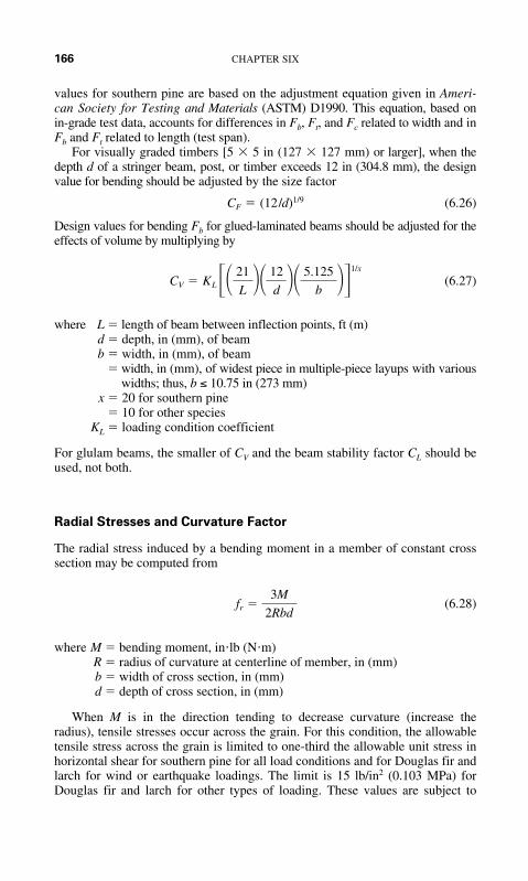
166 CHAPTER SIX
values for southern pine are based on the adjustment equation given in Ameri-can Society for Testing and Materials (ASTM) D1990. This equation, based onin-grade test data, accounts for differences in Fb, Ft, and Fc related to width and inFb and Ft related to length (test span).
For visually graded timbers [5 � 5 in (127 � 127 mm) or larger], when thedepth d of a stringer beam, post, or timber exceeds 12 in (304.8 mm), the designvalue for bending should be adjusted by the size factor
(6.26)
Design values for bending Fb for glued-laminated beams should be adjusted for theeffects of volume by multiplying by
(6.27)
where L � length of beam between inflection points, ft (m)d � depth, in (mm), of beamb � width, in (mm), of beam
� width, in (mm), of widest piece in multiple-piece layups with variouswidths; thus, b 10.75 in (273 mm)
x � 20 for southern pine� 10 for other species
KL � loading condition coefficient
For glulam beams, the smaller of CV and the beam stability factor CL should beused, not both.
Radial Stresses and Curvature Factor
The radial stress induced by a bending moment in a member of constant crosssection may be computed from
(6.28)
where M � bending moment, in�lb (N�m)R � radius of curvature at centerline of member, in (mm)b � width of cross section, in (mm)d � depth of cross section, in (mm)
When M is in the direction tending to decrease curvature (increase theradius), tensile stresses occur across the grain. For this condition, the allowabletensile stress across the grain is limited to one-third the allowable unit stress inhorizontal shear for southern pine for all load conditions and for Douglas fir andlarch for wind or earthquake loadings. The limit is 15 lb/in2 (0.103 MPa) forDouglas fir and larch for other types of loading. These values are subject to
fr �3M
2Rbd
CV � KL �� 21
L �� 12
d �� 5.125
b ��1/x
CF � (12 / d)1/9

TIMBER ENGINEERING FORMULAS 167
modification for duration of load. If these values are exceeded, mechanical rein-forcement sufficient to resist all radial tensile stresses is required.
When M is in the direction tending to increase curvature (decrease theradius), the stress is compressive across the grain. For this condition, the designvalue is limited to that for compression perpendicular to grain for all species.
For the curved portion of members, the design value for wood in bendingshould be modified by multiplication by the following curvature factor:
(6.29)
where t is the thickness of lamination, in (mm); and R is the radius of curvatureof lamination, in (mm). Note that t/R should not exceed 1/100 for hardwoodsand southern pine or 1/125 for softwoods other than southern pine. The curva-ture factor should not be applied to stress in the straight portion of an assembly,regardless of curvature elsewhere.
Bearing Area Factor
Design values for compression perpendicular to the grain Fc� apply to bear-ing surfaces of any length at the ends of a member and to all bearings 6 in(152.4 mm) or more long at other locations. For bearings less than 6 in(152.4 mm) long and at least 3 in (76.2 mm) from the end of a member, Fc�
may be multiplied by the bearing area factor:
(6.30)
where Lb is the bearing length, in (mm) measured parallel to grain. Equation(6.30) yields the values of Cb for elements with small areas, such as plates andwashers, listed in reference data. For round bearing areas, such as washers, Lbshould be taken as the diameter.
Column Stability and Buckling Stiffness Factors
Design values for compression parallel to the grain Ft should be multiplied bythe column stability factor Cp given by Eq. (6.31):
(6.31)
where � design value for compression parallel to the grain multiplied by allapplicable adjustment factors except Cp
FcE �
� modulus of elasticity multiplied by adjustment factorsE�
KcE E�/(Le /d)2
F *c
CP �1 � (FcE /F *
c )
2c� B� 1 � (FcE /Fc
*)
2c �2
�(FcE /F *
c )
c
Cb �Lb � 0.375
Lb
Cc � 1 � 2000 � t
R �2

168 CHAPTER SIX
KcE � 0.3 for visually graded lumber and machine-evaluated lumber� 0.418 for products with a coefficient of variation less than 0.11
c � 0.80 for solid-sawn lumber� 0.85 for round timber piles� 0.90 for glued-laminated timber
For a compression member braced in all directions throughout its length to pre-vent lateral displacement, Cp � 1.0.
The buckling stiffness of a truss compression chord of sawn lumber subjectedto combined flexure and axial compression under dry service conditions maybe increased if the chord is 2 � 4 in (50.8 � 101.6 mm) or smaller and has thenarrow face braced by nailing to plywood sheathing at least in (9.5 mm)thick in accordance with good nailing practice. The increased stiffness may beaccounted for by multiplying the design value of the modulus of elasticity E bythe buckling stiffness factor CT in column stability calculations. When theeffective column length Le, in (mm), is 96 in (2.38 m) or less, CT may be com-puted from
(6.32)
where KM � 2300 for wood seasoned to a moisture content of 19 percent or lessat time of sheathing attachment
� 1200 for unseasoned or partly seasoned wood at time of sheathingattachment
KT � 0.59 for visually graded lumber and machine-evaluated lumber
� 0.82 for products with a coefficient of variation of 0.11 or less
When Le is more than 96 in (2.38 m), CT should be calculated from Eq. (6.32)with Le � 96 in (2.38 m). For additional information on wood trusses with metal-plate connections, see design standards of the Truss Plate Institute, Madison,Wisconsin.
The slenderness ratio RB for beams is defined by
(6.33)
The slenderness ratio should not exceed 50.The effective length Le for Eq. (6.33) is given in terms of unsupported length
of beam in reference data. Unsupported length is the distance between supportsor the length of a cantilever when the beam is laterally braced at the supports toprevent rotation and adequate bracing is not installed elsewhere in the span.When both rotational and lateral displacements are also prevented at intermedi-ate points, the unsupported length may be taken as the distance between pointsof lateral support. If the compression edge is supported throughout the length ofthe beam and adequate bracing is installed at the supports, the unsupportedlength is zero.
RB � BLe d
b2
CT � 1 �KM Le
KT E
3�8

TIMBER ENGINEERING FORMULAS 169
The beam stability factor CL may be calculated from
(6.34)
where � design value for bending multiplied by all applicable adjustmentfactors, except Cfu, CV, and CL
FbE �
� 0.438 for visually graded lumber and machine-evaluated lumber
� 0.609 for products with a coefficient of variation of 0.11 or less
� design modulus of elasticity multiplied by applicable adjustmentfactors
FASTENERS FOR WOOD
Nails and Spikes
The allowable withdrawal load per inch (25.4 mm) of penetration of a commonnail or spike driven into side grain (perpendicular to fibers) of seasoned wood,or unseasoned wood that remains wet, is
(6.35)
where p � allowable load per inch (mm) of penetration into member receivingpoint, lb (N)
D � diameter of nail or spike, in (mm)G � specific gravity of wood, oven dry
The total allowable lateral load for a nail or spike driven into side grain ofseasoned wood is
(6.36)
where p � allowable load per nail or spike, lb (N)D � diameter of nail or spike, in (mm)C � coefficient dependent on group number of wood (see Table 6.1)
Values of C for the four groups into which stress-grade lumber is classified are
Group I: C � 2,040
Group II: C � 1,650
Group III: C � 1,350
Group IV: C � 1,080
p � CD3/2
p � 1,380G5/2D
E�
KbE
KbE E�/R 2B
F *b
CL �1 � (FbE/Fb
*)
1.9� B� 1 � (FbE/Fb
*)
1.9 �2
�FbE /F *
b
0.95

170 CHAPTER SIX
The loads apply where the nail or spike penetrates into the member, receiving itspoint at least 10 diameters for Group I species, 11 diameters for Group IIspecies, 13 diameters for Group III species, and 14 diameters for Group IVspecies. Allowable loads for lesser penetrations are directly proportional to thepenetration, but the penetration must be at least one-third that specified.
Wood Screws
The allowable withdrawal load per inch (mm) of penetration of the threadedportion of a wood screw into side grain of seasoned wood that remains dry is
p � 2,850G2D (6.37)
where p � allowable load per inch (mm) of penetration of threaded portion intomember receiving point, lb (N)
D � diameter of wood screw, in (mm)G � specific gravity of wood, oven dry (see Table 6.1)
Wood screws should not be loaded in withdrawal from end grain.The total allowable lateral load for wood screws driven into the side grain of
seasoned wood which remains dry is
p � CD2 (6.38)
where p � allowable load per wood screw, lb (N)D � diameter of wood screw, in (mm)C � coefficient dependent on group number of wood (Table 6.2)
Values of C for the four groups into which stress-grade lumber is classified are
Group I: C � 4,800
Group II: C � 3,960
Group III: C � 3,240
Group IV: C � 2,520
TABLE 6.2 Specific Gravity and Group Number for CommonSpecies of Lumber
Group SpecificSpecies number gravity, G G2 G5/2
Douglas fir II 0.51 0.260 0.186Pine, southern II 0.59 0.348 0.267Hemlock, western III 0.44 0.194 0.128Hemlock, eastern IV 0.43 0.185 0.121Pine, Norway III 0.47 0.221 0.151Redwood III 0.42 0.176 0.114Spruce IV 0.41 0.168 0.108
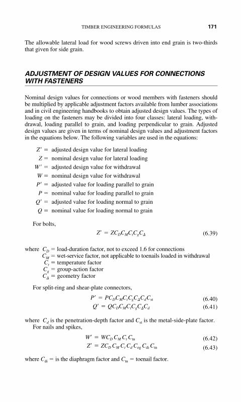
TIMBER ENGINEERING FORMULAS 171
The allowable lateral load for wood screws driven into end grain is two-thirdsthat given for side grain.
ADJUSTMENT OF DESIGN VALUES FOR CONNECTIONSWITH FASTENERS
Nominal design values for connections or wood members with fasteners shouldbe multiplied by applicable adjustment factors available from lumber associationsand in civil engineering handbooks to obtain adjusted design values. The types ofloading on the fasteners may be divided into four classes: lateral loading, with-drawal, loading parallel to grain, and loading perpendicular to grain. Adjusteddesign values are given in terms of nominal design values and adjustment factorsin the equations below. The following variables are used in the equations:
Z� � adjusted design value for lateral loading
Z � nominal design value for lateral loading
W � � adjusted design value for withdrawal
W � nominal design value for withdrawal
P� � adjusted value for loading parallel to grain
P � nominal value for loading parallel to grain
Q� � adjusted value for loading normal to grain
Q � nominal value for loading normal to grain
For bolts,
(6.39)
where CD � load-duration factor, not to exceed 1.6 for connectionsCM � wet-service factor, not applicable to toenails loaded in withdrawalCt � temperature factorCg � group-action factorC� � geometry factor
For split-ring and shear-plate connectors,
(6.40)(6.41)
where Cd is the penetration-depth factor and Cst is the metal-side-plate factor.For nails and spikes,
(6.42)
(6.43)
where Cdi � is the diaphragm factor and Ctn � toenail factor.
Z� � ZCD CM Ct Cd Ceg Cdi Ctn
W� � WCD CM Ct Ctn
Q� � QCDCMCtCgC�Cd
P� � PCDCMCtCgC�CdCst
Z� � ZCDCMCtCgC�

172 CHAPTER SIX
For wood screws,
(6.44)
(6.45)
where Ceg is the end-grain factor.For lag screws,
(6.46)(6.47)
For metal plate connectors,
(6.48)
For drift bolts and drift pins,
(6.49)(6.50)
For spike grids,
(6.51)
ROOF SLOPE TO PREVENT PONDING
Roof beams should have a continuous upward slope equivalent to in/ft(20.8 mm/m) between a drain and the high point of a roof, in addition tominimum recommended camber to avoid ponding. When flat roofs haveinsuffic-ient slope for drainage (less than in/ft) (20.8 mm/m) the stiffnessof supporting members should be such that a 5-lb/ft2 (239.4 N/mm2) loadcauses no more than -in (12.7 mm) deflection.
Because of ponding, snow loads or water trapped by gravel stops, parapetwalls, or ice dams magnify stresses and deflections from existing roof loads* by
(6.52)
where Cp � factor for multiplying stresses and deflections under existing loads todetermine stresses and deflections under existing loads plus ponding
W � weight of 1 in (25.4 mm) of water on roof area supported by beam, lb (N)L � span of beam, in (mm)E � modulus of elasticity of beam material, lb/in2 (MPa)I � moment of inertia of beam, in4 (mm4)
Cp �1
1 � W�L3/ 4EI
1�2
1�4
1�4
Z� � ZCDCMCtC�
Z� � ZCDCMCtCgC�CdCeg
W� � WCDCMCtCeg
Z� � ZCDCMCt
Z� � ZCDCMCtCgC�CdCeg
W� � WCDCMCtCeg
Z� � ZCDCMCtCdCeg
W� � WCDCMCt
*Kuenzi and Bohannan, “Increases in Deflection and Stresses Caused by Ponding of Water onRoofs,” Forest Products Laboratory, Madison, Wisconsin.

TIMBER ENGINEERING FORMULAS 173
BENDING AND AXIAL TENSION
Members subjected to combined bending and axial tension should be propor-tioned to satisfy the interaction equations
(6.53)
and
(6.54)
where ft � tensile stress due to axial tension acting alonefb � bending stress due to bending moment alone
� design value for tension multiplied by applicable adjustment factors
� design value for bending multiplied by applicable adjustment fac-tors except CL
� design value for bending multiplied by applicable adjustment factorsexcept CV
The load duration factor CD associated with the load of shortest duration in acombination of loads with differing duration may be used to calculate and
. All applicable load combinations should be evaluated to determine the criti-cal load combination.
BENDING AND AXIAL COMPRESSION
Members subjected to a combination of bending and axial compression (beamcolumns) should be proportioned to satisfy the interaction equation
(6.55)
where fc � compressive stress due to axial compression acting alone� design value for compression parallel to grain multiplied by applic-
able adjustment factors, including the column stability factorfb1 � bending stress for load applied to the narrow face of the memberfb2 � bending stress for load applied to the wide face of the member
� design value for bending for load applied to the narrow face of themember multiplied by applicable adjustment factors, including thecolumn stability factor
� design value for bending for load applied to the wide face of themember multiplied by applicable adjustment factors, includingthe column stability factor
F�b2
F�b1
F�c
�fb2
[1 � ( fc /FcE2) � ( fb1/FbE)2]F�b2� 1
� fc
F�c�
2
�fb1
[1 � ( fc /FcE1)]F�b1
F b*
F�t
F **b
F *b
F�t
( fb � ft)
F **b
� 1
ft
Fc��
fb
F *b
� 1

174 CHAPTER SIX
For either uniaxial or biaxial bending, fc should not exceed
(6.56)
where E� is the modulus of elasticity multiplied by adjustment factors. Also, forbiaxial bending, fc should not exceed
(6.57)
and fb1 should not be more than
(6.58)
where d1 is the width of the wide face and d2 is the width of the narrow face.Slenderness ratio RB for beams is given earlier in this section. KbE is definedearlier in this section. The effective column lengths Le1 for buckling in the d1 direc-tion and Le2 for buckling in the d2 direction, E�, FcE1, and FcE2 should be determinedas shown earlier.
As for the case of combined bending and axial tension, , , and should be adjusted for duration of load by applying CD.
Nomenclature for Formulas given in Eqs. (6.59) through (6.57):
Q � allowable load, lbP � ultimate load, lbA � section area of column, sq inL � length of column, inr � least radius of gyration of column section, in
Su � ultimate strength, psiSy � yield point or yield strength of material, psiE � modulus of elasticity of material, psim � factor of safety
(L/r)� � critical slenderness ratio
SOLID RECTANGULAR OR SQUARE COLUMNS WITH FLAT ENDS*
For select structural-grade lumber in general structural use under continuously dryconditions, the following formulas can be used for the allowable unit load, Q/A:
(6.59)Q
A� S�1 �
1
3 �L
Kd �4
�up to L
d� K � 0.64B
E
S
F�b2F�b1F�c
FbE �KbE E�
R2B
FcE2 �KcE E�
(Le2 /d2)2
FcE1 �KcE E�
(Le1/d1)2
*Roark—“Formulas for Stress and Strain,” McGraw-Hill.
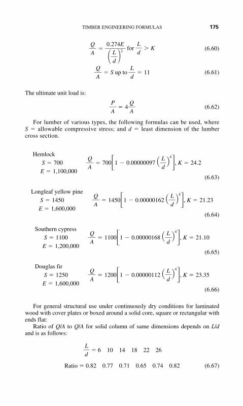
TIMBER ENGINEERING FORMULAS 175
(6.60)
(6.61)
The ultimate unit load is:
(6.62)
For lumber of various types, the following formulas can be used, whereS � allowable compressive stress; and d � least dimension of the lumbercross section.
(6.63)
(6.64)
(6.65)
(6.66)
For general structural use under continuously dry conditions for laminatedwood with cover plates or boxed around a solid core, square or rectangular withends flat:
Ratio of Q/A to Q/A for solid column of same dimensions depends on L/dand is as follows:
� 6 10 14 18 22 26
Ratio � 0.82 0.77 0.71 0.65 0.74 0.82 (6.67)
L
d
Q
A� 1200�1 � 0.00000112 � L
d�
4
�, K � 23.35
Douglas fir
S � 1250
E � 1,600,000
Q
A� 1100�1 � 0.00000168 � L
d�
4
�, K � 21.10
Southern cypress
S � 1100
E � 1,200,000
Q
A� 1450�1 � 0.00000162 � L
d�
4
�, K � 21.23
Longleaf yellow pine
S � 1450
E � 1,600,000
Q
A� 700�1 � 0.00000097 � L
d�
4
�, K � 24.2
Hemlock
S � 700
E � 1,100,000
P
A� 4
Q
A
Q
A� S up to
L
d� 11
Q
A�
0.274E
� L
d �2 for
L
d K

176 CHAPTER SIX
For solid circular columns with ends flat in general structural use under con-tinuously dry conditions:
Q/A is same as for square column of equal area. For tapered round column,d and A are taken as for section distant 1/3 L from smaller end. Q/A at smallend must not exceed S.
Note: Where numeric constants appear in formulas, compute in USCS val-ues and then convert to SI using the conversion factors in Chap. 1.

CHAPTER 7
177
SURVEYINGFORMULAS
UNITS OF MEASUREMENT
Units of measurement used in past and present surveys are
For construction work: feet, inches, fractions of inches (m, mm)
For most surveys: feet, tenths, hundredths, thousandths (m, mm)
For National Geodetic Survey (NGS) control surveys: meters, 0.1, 0.01, 0.001 m
The most-used equivalents are
1 meter � 39.37 in (exactly) � 3.2808 ft
1 rod � 1 pole � 1 perch � ft (5.029 m)
1 engineer’s chain � 100 ft � 100 links (30.48 m)
1 Gunter’s chain � 66 ft (20.11 m) � 100 Gunter’s links (lk) � 4 rods � mi(0.020 km)
1 acre � 100,000 sq (Gunter’s) links � 43,560 ft2 � 160 rods2 � 10 sq(Gunter’s) chains � 4046.87 m2 � 0.4047 ha
1 rood � acre (1011.5 m2) � 40 rods2 (also local unit � to 8 yd) (5.029 to 7.315 m)
1 ha � 10,000 m2 � 107,639.10 ft2 � 2.471 acres
1 arpent � about 0.85 acre, or length of side of 1 square arpent (varies) (about3439.1 m2)
1 statute mi � 5280 ft � 1609.35 m
1 mi2 � 640 acres (258.94 ha)
1 nautical mi (U.S.) � 6080.27 ft � 1853.248 m
1 fathom � 6 ft (1.829 m)
1 cubit � 18 in (0.457 m)
1 vara � 33 in (0.838 m) (Calif.), in (0.851 m) (Texas), varies
1 degree � circle � 60 min � 3600 s � 0.01745 rad
sin 1� � 0.01745241
1�360
331�3
51�23�4
1�80
161�2

178 CHAPTER SEVEN
1 rad � 57� 17� 44.8� or about 57.30�
1 grad (grade) � circle � quadrant � 100 centesimal min � 104 cen-tesimals (French)
1 mil � circle � 0.05625�
1 military pace (milpace) � ft (0.762 m)
THEORY OF ERRORS
When a number of surveying measurements of the same quantity have beenmade, they must be analyzed on the basis of probability and the theory oferrors. After all systematic (cumulative) errors and mistakes have been elimi-nated, random (compensating) errors are investigated to determine the mostprobable value (mean) and other critical values. Formulas determined fromstatistical theory and the normal, or Gaussian, bell-shaped probability distrib-ution curve, for the most common of these values follow.
Standard deviation of a series of observations is
(7.1)
where d � residual (difference from mean) of single observation and n � num-ber of observations.
The probable error of a single observation is
(7.2)
(The probability that an error within this range will occur is 0.50.)The probability that an error will lie between two values is given by the
ratio of the area of the probability curve included between the values to the totalarea. Inasmuch as the area under the entire probability curve is unity, there is a100 percent probability that all measurements will lie within the range of thecurve.
The area of the curve between � �s is 0.683; that is, there is a 68.3 percentprobability of an error between � �s in a single measurement. This error rangeis also called the one-sigma or 68.3 percent confidence level. The area of thecurve between � 2�s is 0.955. Thus, there is a 95.5 percent probability of anerror between � 2�s and � 2�s that represents the 95.5 percent error (two-sigma or 95.5 percent confidence level). Similarly, � 3�s is referred to as the99.7 percent error (three-sigma or 99.7 percent confidence level). For practicalpurposes, a maximum tolerable level often is assumed to be the 99.9 percenterror. Table 7.1 indicates the probability of occurrence of larger errors in a sin-gle measurement.
The probable error of the combined effects of accidental errors from differ-ent causes is
(7.3)Esum � 2E21 � E2
2 � E23 � � � �
PEs � �0.6745�s
�s � � Bd 2
n � 1
21�2
1�6400
1�1001�400

SURVEYING FORMULAS 179
where E1, E2, E3 . . . are probable errors of the separate measurements.Error of the mean is
(7.4)
where Es � specified error of a single measurement.Probable error of the mean is
(7.5)
MEASUREMENT OF DISTANCE WITH TAPES
Reasonable precisions for different methods of measuring distances are
Pacing (ordinary terrain): to
Taping (ordinary steel tape): to (Results can be improved by use oftension apparatus, transit alignment, leveling.)
Baseline (invar tape): to
Stadia: to (with special procedures)
Subtense bar: to (for short distances, with a 1-s theodolite, averag-ing angles taken at both ends)
Electronic distance measurement (EDM) devices have been in use since themiddle of the twentieth century and have now largely replaced steel tape mea-surements on large projects. The continued development, and the resulting dropin prices, are making their use widespread. A knowledge of steel-taping errorsand corrections remains important, however, because use of earlier survey datarequires a knowledge of how the measurements were made, common sources forerrors, and corrections that were typically required.
1�70001�1000
1�5001�300
1�1,000,0001�50,000
1�10,0001�1000
1�1001�50
PEm �PEs
�n� �0.6745B
d 2
n(n � 1)
Em �Esum
n�
Es�n
n�
Es
�n
TABLE 7.1 Probability of Error in a Single Measurement
ProbabilityConfidence of larger
Error level, % error
Probable (0.6745�s) 50 1 in 2Standard deviation (�s) 68.3 1 in 390% (1.6449�s) 90 1 in 102�s or 95.5% 95.5 1 in 203�s or 97.7% 99.7 1 in 370Maximum (3.29�s) 99.9� 1 in 1000

180 CHAPTER SEVEN
For ordinary taping, a tape accurate to 0.01 ft (0.00305 m) should be used. Thetension of the tape should be about 15 lb (66.7 N). The temperature should bedetermined within 10°F (5.56°C); and the slope of the ground, within 2 percent;and the proper corrections, applied. The correction to be applied for tempera-ture when using a steel tape is
(7.6)
The correction to be made to measurements on a slope is
(7.7)
or (7.8)
or (7.9)
where Ct � temperature correction to measured length, ft (m)Ch � correction to be subtracted from slope distance, ft (m)
s � measured length, ft (m)T � temperature at which measurements are made, �F (�C)
T0 � temperature at which tape is standardized, �F (�C)h � difference in elevation at ends of measured length, ft (m)� � slope angle, degree
In more accurate taping, using a tape standardized when fully supported through-out, corrections should also be made for tension and for support conditions. The cor-rection for tension is
(7.10)
The correction for sag when not fully supported is
(7.11)
where Cp � tension correction to measured length, ft (m)Cs � sag correction to measured length for each section of unsupported
tape, ft (m)Pm � actual tension, lb (N)Ps � tension at which tape is standardized, lb (N) (usually 10 lb) (44.4 N)S � cross-sectional area of tape, in2 (mm2)E � modulus of elasticity of tape, lb/in2 (MPa) [29 million lb/in2 (MPa) for
steel] (199,955 MPa)w � weight of tape, lb/ft (kg/m)L � unsupported length, ft (m)
Slope Corrections
In slope measurements, the horizontal distance H � L cos x, where L �slope distance and x � vertical angle, measured from the horizontal—a simple
Cs �w 2L3
24P 2m
Cp �(Pm � Ps)s
SE
� h2/2s approximate
� 0.00015s�2 approximate
Ch � s (1 � cos �) exact
Ct � 0.0000065s(T � T0)

SURVEYING FORMULAS 181
hand calculator operation. For slopes of 10 percent or less, the correction to beapplied to L for a difference d in elevation between tape ends, or for a horizon-tal offset d between tape ends, may be computed from
(7.12)
For a slope greater than 10 percent, Cs may be determined from
(7.13)
Temperature Corrections
For incorrect tape length:
(7.14)
For nonstandard tension:
(7.15)
where A � cross-sectional area of tape, in2 (mm2); and E � modulus of elas-ticity � 29,000,00 lb/ in2 for steel (199,955 MPa).
For sag correction between points of support, ft (m):
(7.16)
where w � weight of tape per foot, lb (N)Ls � unsupported length of tape, ft (m)P � pull on tape, lb (N)
Orthometric Correction
This is a correction applied to preliminary elevations due to flattening of theearth in the polar direction. Its value is a function of the latitude and elevationof the level circuit.
Curvature of the earth causes a horizontal line to depart from a level sur-face. The departure Cf, ft; or Cm, (m), may be computed from
(7.17)
(7.18)Cm � 0.0785K2
Cf � 0.667M 2 � 0.0239F 2
C � �w2L3
s
24P2
Ct �(applied pull � standard tension)L
AE
Ct �(actual tape length � nominal tape length)L
nominal tape length
Cs �d 2
2L�
d 4
8L3
Cs �d 2
2L

182 CHAPTER SEVEN
where M, F, and K are distances in miles, thousands of feet, and kilometers,respectively, from the point of tangency to the earth.
Refraction causes light rays that pass through the earth’s atmosphere tobend toward the earth’s surface. For horizontal sights, the average angular dis-placement (like the sun’s diameter) is about 32 min. The displacement Rf, ft, orRm, m, is given approximately by
(7.19)
(7.20)
To obtain the combined effect of refraction and curvature of the earth, subtractRf from Cf or Rm from Cm.
Borrow-pit or cross-section leveling produces elevations at the corners ofsquares or rectangles with sides that are dependent on the area to be covered,type of terrain, and accuracy desired. For example, sides may be 10, 20, 40,50, or 100 ft (3.048, 6.09, 12.19, 15.24, or 30.48 m). Contours can be locatedreadily, but topographic features, not so well. Quantities of material to beexcavated or filled are computed, in yd3 (m3), by selecting a grade elevation orfinal ground elevation, computing elevation differences for the corners, andsubstituting in
(7.21)
where n � number of times a particular corner enters as part of a division blockx � difference in ground and grade elevation for each corner, ft (m)A � area of each block, ft2 (m2)
VERTICAL CONTROL
The NGS provides vertical control for all types of surveys. NGS furnishesdescriptions and elevations of bench marks on request. As given in “Standardsand Specifications for Geodetic Control Networks,” Federal Geodetic ControlCommittee, the relative accuracy C, mm, required between directly connectedbench marks for the three orders of leveling is
First order: for Class I and for Class II (7.22)
Second order: for Class I and for Class II (7.23)
Third order: (7.24)
where K is the distance between bench marks, km.
C � 2.02K
1.32KC � 1.02K
0.72KC � 0.52K
Q �nxA
108
Rm � 0.011K2
Rf � 0.093M2 � 0.0033F 2

SURVEYING FORMULAS 183
STADIA SURVEYING
In stadia surveying, a transit having horizontal stadia crosshairs above andbelow the central horizontal crosshair is used. The difference in the rod read-ings at the stadia crosshairs is termed the rod intercept. The intercept maybe converted to the horizontal and vertical distances between the instrumentand the rod by the following formulas:
(7.25)
(7.26)
where H � horizontal distance between center of transit and rod, ft (m)V � vertical distance between center of transit and point on rod inter-
sected by middle horizontal crosshair, ft (m)K � stadia factor (usually 100)i � rod intercept, ft (m)a � vertical inclination of line of sight, measured from the horizontal,
degreef � c � instrument constant, ft (m) (usually taken as 1 ft) (0.3048 m)
In the use of these formulas, distances are usually calculated to the foot (meter)and differences in elevation to tenths of a foot (meter).
Figure 7.1 shows stadia relationships for a horizontal sight with theolder type of external-focusing telescope. Relationships are comparable forthe internal-focusing type.
For horizontal sights, the stadia distance, ft, (m) (from instrument spindle torod), is
(7.27)D � R� f
i� C�
V �1
2Ki (sin 2a) � ( f � c) sin a
H � Ki (cos a)2 � ( f � c) cos a
f1 f2
cC
a´
b´
mi
a
bF
D
f dB
A
R
FIGURE 7.1 Distance D is measured with an external-focusing telescope by determininginterval R intercepted on a rod AB by two horizontal sighting wires a and b.

184 CHAPTER SEVEN
where R � intercept on rod between two sighting wires, ft (m)f � focal length of telescope, ft (m) (constant for specific instrument)i � distance between stadia wires, ft (m)
C � f � c (7.28)
c � distance from center of spindle to center of objective lens, ft (m)
C is called the stadia constant, although c and C vary slightly.The value of f/i, the stadia factor, is set by the manufacturer to be about 100,
but it is not necessarily 100.00. The value should be checked before use onimportant work, or when the wires or reticle are damaged and replaced.
PHOTOGRAMMETRY
Photogrammetry is the art and science of obtaining reliable measurements byphotography (metric photogrammetry) and qualitative evaluation of image data(photo interpretation). It includes use of terrestrial, close-range, aerial, vertical,oblique, strip, and space photographs along with their interpretation.
Scale formulas are as follows:
(7.29)
(7.30)
where f � focal length of lens, in (m)H � flying height of airplane above datum (usually mean sea level), ft (m)h1 � elevation of point, line, or area with respect to datum, ft (m)
Photo scale �ab
AB�
f
H � h1
Photo scale
Map scale�
photo distance
map distance

CHAPTER 8
185
SOIL ANDEARTHWORKFORMULAS
PHYSICAL PROPERTIES OF SOILS
Basic soil properties and parameters can be subdivided into physical, index, andengineering categories. Physical soil properties include density, particle size anddistribution, specific gravity, and water content.
The water content w of a soil sample represents the weight of free watercontained in the sample expressed as a percentage of its dry weight.
The degree of saturation S of the sample is the ratio, expressed as percent-age, of the volume of free water contained in a sample to its total volume ofvoids Vv.
Porosity n, which is a measure of the relative amount of voids, is the ratio ofvoid volume to the total volume V of soil:
(8.1)
The ratio of Vv to the volume occupied by the soil particles Vs defines the voidratio e. Given e, the degree of saturation may be computed from
(8.2)
where Gs represents the specific gravity of the soil particles. For most inorganicsoils, Gs is usually in the range of 2.67 � 0.05.
The dry unit weight �d of a soil specimen with any degree of saturation maybe calculated from
(8.3)
where �w is the unit weight of water and is usually taken as 62.4 lb/ft3 (1001 kg/m3)for freshwater and 64.0 lb/ft3 (1026.7 kg/m3) for seawater.
�d ��w Gs S
1 � wGs
S �wGs
e
n �Vv
V
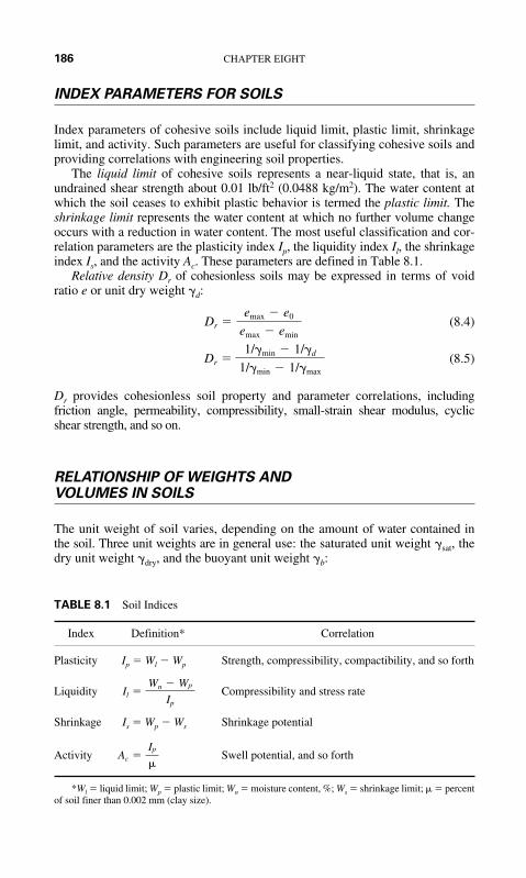
186 CHAPTER EIGHT
INDEX PARAMETERS FOR SOILS
Index parameters of cohesive soils include liquid limit, plastic limit, shrinkagelimit, and activity. Such parameters are useful for classifying cohesive soils andproviding correlations with engineering soil properties.
The liquid limit of cohesive soils represents a near-liquid state, that is, anundrained shear strength about 0.01 lb/ft2 (0.0488 kg/m2). The water content atwhich the soil ceases to exhibit plastic behavior is termed the plastic limit. Theshrinkage limit represents the water content at which no further volume changeoccurs with a reduction in water content. The most useful classification and cor-relation parameters are the plasticity index Ip, the liquidity index Il, the shrinkageindex Is, and the activity Ac. These parameters are defined in Table 8.1.
Relative density Dr of cohesionless soils may be expressed in terms of voidratio e or unit dry weight �d:
(8.4)
(8.5)
Dr provides cohesionless soil property and parameter correlations, includingfriction angle, permeability, compressibility, small-strain shear modulus, cyclicshear strength, and so on.
RELATIONSHIP OF WEIGHTS AND VOLUMES IN SOILS
The unit weight of soil varies, depending on the amount of water contained inthe soil. Three unit weights are in general use: the saturated unit weight �sat, thedry unit weight �dry, and the buoyant unit weight �b:
Dr �1/�min � 1/�d
1/�min � 1/�max
Dr �emax � e0
emax � emin
TABLE 8.1 Soil Indices
Index Definition* Correlation
Plasticity Ip � Wl � Wp Strength, compressibility, compactibility, and so forth
Liquidity Compressibility and stress rate
Shrinkage Is � Wp � Ws Shrinkage potential
Activity Swell potential, and so forth
*Wl � liquid limit; Wp � plastic limit; Wn � moisture content, %; Ws � shrinkage limit; � � percentof soil finer than 0.002 mm (clay size).
Ac �Ip
�
Il �Wn � Wp
Ip

SOIL AND EARTHWORK FORMULAS 187
(8.6)
(8.7)
(8.8)
Unit weights are generally expressed in pound per cubic foot or gram per cubiccentimeter. Representative values of unit weights for a soil with a specific grav-ity of 2.73 and a void ratio of 0.80 are
(8.9)
(8.10)
(8.11)
The symbols used in the three preceding equations and in Fig. 8.1 are
G � specific gravity of soil solids (specific gravity of quartz is 2.67; formajority of soils specific gravity ranges between 2.65 and 2.85; organicsoils would have lower specific gravities)
�0 � unit weight of water, 62.4 lb/ft3 (1.0 g/cm3)
e � voids ratio, volume of voids in mass of soil divided by volume of solidsin same mass; also equal to n / (1 � n), where n is porosity—volume ofvoids in mass of soil divided by total volume of same mass
S � degree of saturation, volume of water in mass of soil divided by volumeof voids in same mass
w � water content, weight of water in mass of soil divided by weight ofsolids in same mass; also equal to Se /G
�b � 60 lb/ft3 � 0.96 g/cm3
�dry � 95 lb/ft3 � 1.52 g/cm3
�sat � 122 lb/ft3 � 1.96 g/cm3
�b �(G � 1)�0
1 � e S � 100%
�dry �G�0
(1 � e) S � 0%
�sat �(G � e)�0
1 � e�
(1 � w)G�0
1 � e S � 100%
Total volume (solids + water + gas) = 1
Gas
Water
Solids1=
1 +
e
V(s
olid
s)
W(t
otal
) (f
or u
nitV
) =
γf
V =
1
V(v
oids
)
V(w
ater
)
W(w
ater
)W
(sol
ids)
e=
1 +
e
Se=
1 +
e
1G
γ 0γ 0
=1
+ e
G+
Seγ 0
=1
+ e
1 +
wG
γ 0=
1 +
e
Se=
1 +
e
FIGURE 8.1 Relationship of weights and volumes in soil.

188 CHAPTER EIGHT
INTERNAL FRICTION AND COHESION
The angle of internal friction for a soil is expressed by
(8.12)
where � � angle of internal frictiontan � � coefficient of internal friction
� � normal force on given plane in cohesionless soil mass! � shearing force on same plane when sliding on plane is
impending
For medium and coarse sands, the angle of internal friction is about 30° to 35°.The angle of internal friction for clays ranges from practically 0° to 20°.
The cohesion of a soil is the shearing strength that the soil possesses byvirtue of its intrinsic pressure. The value of the ultimate cohesive resis-tance of a soil is usually designated by c. Average values for c are given inTable 8.2.
VERTICAL PRESSURES IN SOILS
The vertical stress in a soil caused by a vertical, concentrated surface load maybe determined with a fair degree of accuracy by the use of elastic theory. Twoequations are in common use, the Boussinesq and the Westergaard. The Boussi-nesq equation applies to an elastic, isotropic, and homogeneous mass thatextends infinitely in all directions from a level surface. The vertical stress at apoint in the mass is
(8.13)�z �3P
2 z2 �1 � � r
z �2
�5/2
tan � �!
�
TABLE 8.2 Cohesive Resistance of Various Soil Types
Cohesion c
General soil type lb/ft2 (kPa)
Almost-liquid clay 100 (4.8)Very soft clay 200 (9.6)Soft clay 400 (19.1)Medium clay 1000 (47.8)Damp, muddy sand 400 (19.1)

SOIL AND EARTHWORK FORMULAS 189
The Westergaard equation applies to an elastic material laterally reinforcedwith horizontal sheets of negligible thickness and infinite rigidity, which preventthe mass from undergoing lateral strain. The vertical stress at a point in themass, assuming a Poisson’s ratio of zero, is
(8.14)
where �z � vertical stress at a point, lb/ft2 (kPa)P � total concentrated surface load, lb (N)z � depth of point at which �z acts, measured vertically downward
from surface, ft (m)r � horizontal distance from projection of surface load P to point at
which �z acts, ft (m)
For values of r/z between 0 and 1, the Westergaard equation gives stressesappreciably lower than those given by the Boussinesq equation. For values ofr /z greater than 2.2, both equations give stresses less than P /100z2.
LATERAL PRESSURES IN SOILS, FORCES ON RETAINING WALLS
The Rankine theory of lateral earth pressures, used for estimating approxi-mate values for lateral pressures on retaining walls, assumes that the pres-sure on the back of a vertical wall is the same as the pressure that wouldexist on a vertical plane in an infinite soil mass. Friction between the walland the soil is neglected. The pressure on a wall consists of (1) the lateralpressure of the soil held by the wall, (2) the pressure of the water (if any)behind the wall, and (3) the lateral pressure from any surcharge on the soilbehind the wall.
Symbols used in this section are as follows:
� � unit weight of soil, lb / ft3 (kg/m3) (saturated unit weight, dry unitweight, or buoyant unit weight, depending on conditions)
P � total thrust of soil, lb / linear ft (kg/ linear m) of wall
H � total height of wall, ft (m)
� � angle of internal friction of soil, degree
i � angle of inclination of ground surface behind wall with horizontal;also angle of inclination of line of action of total thrust P and pres-sures on wall with horizontal
KA � coefficient of active pressure
KP � coefficient of passive pressure
c � cohesion, lb/ft2 (kPa)
�z �P
z2 �1 � 2 � r
z �2
�3/2

190 CHAPTER EIGHT
LATERAL PRESSURE OF COHESIONLESS SOILS
For walls that retain cohesionless soils and are free to move an appreciableamount, the total thrust from the soil is
(8.15)
When the surface behind the wall is level, the thrust is
(8.16)
where (8.17)
The thrust is applied at a point H /3 above the bottom of the wall, and the pressuredistribution is triangular, with the maximum pressure of 2P /H occurring at thebottom of the wall.
For walls that retain cohesionless soils and are free to move only a slightamount, the total thrust is 1.12P, where P is as given earlier. The thrust isapplied at the midpoint of the wall, and the pressure distribution is trapezoidal,with the maximum pressure of 1.4P /H extending over the middle six-tenth ofthe height of the wall.
For walls that retain cohesionless soils and are completely restrained (veryrare), the total thrust from the soil is
(8.18)
When the surface behind the wall is level, the thrust is
(8.19)
where (8.20)
The thrust is applied at a point H /3 above the bottom of the wall, and the pres-sure distribution is triangular, with the maximum pressure of 2P /H occurringat the bottom of the wall.
KP � �tan �45���
2 ��2
P � 1�2�H 2KP
P �1
2�H 2 cos i
cos i � 2(cos i)2 � (cos �)2
cos i � 2(cos i)2 � (cos �)2
KA � �tan �45���
2 ��2
P � 1�2� H 2KA
P �1
2�H 2 cos i
cos i � 2(cos i)2 � (cos �)2
cos i � 2(cos i)2 � (cos �)2

SOIL AND EARTHWORK FORMULAS 191
LATERAL PRESSURE OF COHESIVE SOILS
For walls that retain cohesive soils and are free to move a considerable amountover a long period of time, the total thrust from the soil (assuming a level sur-face) is
(8.21)
or, because highly cohesive soils generally have small angles of internalfriction,
(8.22)
The thrust is applied at a point somewhat below H /3 from the bottom of thewall, and the pressure distribution is approximately triangular.
For walls that retain cohesive soils and are free to move only a smallamount or not at all, the total thrust from the soil is
(8.23)
because the cohesion would be lost through plastic flow.
WATER PRESSURE
The total thrust from water retained behind a wall is
(8.24)
where H � height of water above bottom of wall, ft (m); and �0 � unit weight ofwater, lb/ft3 62.4 lb/ft3 (1001 kg/m3) for freshwater and 64 lb/ft3 (1026.7 kg/m3)for saltwater.
The thrust is applied at a point H /3 above the bottom of the wall, and thepressure distribution is triangular, with the maximum pressure of 2P /H occur-ring at the bottom of the wall. Regardless of the slope of the surface behind thewall, the thrust from water is always horizontal.
LATERAL PRESSURE FROM SURCHARGE
The effect of a surcharge on a wall retaining a cohesionless soil or an unsatu-rated cohesive soil can be accounted for by applying a uniform horizontal loadof magnitude KAp over the entire height of the wall, where p is the surcharge inpound per square foot (kilopascal). For saturated cohesive soils, the full valueof the surcharge p should be considered as acting over the entire height of thewall as a uniform horizontal load. KA is defined earlier.
P � 1�2�0H 2
P � 1�2�H 2KP
P � 1�2�H 2 � 2cH
P � 1�2�H 2KA � 2cH �KA

192 CHAPTER EIGHT
STABILITY OF SLOPES
Cohesionless Soils
A slope in a cohesionless soil without seepage of water is stable if
(8.25)
With seepage of water parallel to the slope, and assuming the soil to be satu-rated, an infinite slope in a cohesionless soil is stable if
(8.26)
where i � slope of ground surface� � angle of internal friction of soil
�b, �sat � unit weights, lb/ft3 (kg/m3)
Cohesive Soils
A slope in a cohesive soil is stable if
(8.27)
where H � height of slope, ft (m)C � cohesion, lb/ft2 (kg/m2)� � unit weight, lb/ft3 (kg/m3)N � stability number, dimensionless
For failure on the slope itself, without seepage water,
(8.28)
Similarly, with seepage of water,
(8.29)
When the slope is submerged, � is the angle of internal friction of the soiland � is equal to �b. When the surrounding water is removed from a submergedslope in a short time (sudden drawdown), � is the weighted angle of internalfriction, equal to (�b /�sat)�, and � is equal to �sat.
BEARING CAPACITY OF SOILS
The approximate ultimate bearing capacity under a long footing at the surfaceof a soil is given by Prandtl’s equation as
N � (cos i)2 �tan i � � �b
�sat� tan ��
N � (cos i)2 (tan i � tan �)
H �C
�N
tan i � � �b
�sat� tan �
i � �

SOIL AND EARTHWORK FORMULAS 193
(8.30)
where qu � ultimate bearing capacity of soil, lb/ft2 (kg/m2)c � cohesion, lb/ft2 (kg/m2)� � angle of internal friction, degree
�dry � unit weight of dry soil, lb/ft3 (kg/m3)b � width of footing, ft (m)d � depth of footing below surface, ft (m)
Kp � coefficient of passive pressure
�
e � 2.718 . . .
For footings below the surface, the ultimate bearing capacity of the soil maybe modified by the factor 1 � Cd /b. The coefficient C is about 2 for cohesion-less soils and about 0.3 for cohesive soils. The increase in bearing capacity withdepth for cohesive soils is often neglected.
SETTLEMENT UNDER FOUNDATIONS
The approximate relationship between loads on foundations and settlement is
(8.31)
where q � load intensity, lb/ft2 (kg/m2)P � settlement, in (mm)d � depth of foundation below ground surface, ft (m)b � width of foundation, ft (m)
C1 � coefficient dependent on internal frictionC2 � coefficient dependent on cohesion
The coefficients C1 and C2 are usually determined by bearing-plate loading tests.
SOIL COMPACTION TESTS
The sand-cone method is used to determine in the field the density of com-pacted soils in earth embankments, road fill, and structure backfill, as well asthe density of natural soil deposits, aggregates, soil mixtures, or other similarmaterials. It is not suitable, however, for soils that are saturated, soft, or friable(crumble easily).
q
P� C1 �1 �
2d
b � �C2
b
�tan�45 ��
2 ��2
qu � � c
tan � � �1
2�dry b2Kp (Kp e tan � � 1)

194 CHAPTER EIGHT
Characteristics of the soil are computed from
(8.32)
(8.33)
(8.34)
(8.35)
(8.36)
Maximum density is found by plotting a density–moisture curve.
Load-Bearing Test
One of the earliest methods for evaluating the in situ deformability ofcoarse-grained soils is the small-scale load-bearing test. Data developedfrom these tests have been used to provide a scaling factor to express the set-tlement � of a full-size footing from the settlement �1 of a 1-ft2 (0.0929-m2)plate. This factor �/�1 is given as a function of the width B of the full-sizebearing plate as
(8.37)
From an elastic half-space solution, E�s can be expressed from results of a plateload test in terms of the ratio of bearing pressure to plate settlement kv as
(8.38)
where � represents Poisson’s ratio, usually considered to range between0.30 and 0.40. The E�s equation assumes that �1 is derived from a rigid, 1-ft(0.3048-m)-diameter circular plate and that B is the equivalent diameter ofthe bearing area of a full-scale footing. Empirical formulations, such as the�/�1 equation, may be significantly in error because of the limited footing-size range used and the large scatter of the database. Furthermore, considera-tion is not given to variations in the characteristics and stress history of thebearing soils.
Es� �kv (1 � �2) /4
4B/(1 � B)2
�
�1 � � 2B
1 � B �2
% Compaction �100(dry density)
max dry density
Dry density �field density
1 � % moisture/100
Field density, lb/ft 3 (kg /m3) �weight of soil, lb (kg)
volume of soil, ft3 (m3)
% Moisture �100(weight of moist soil � weight of dry soil)
weight of dry soil
�weight of sand filling hole, lb (kg)
density of sand, lb/ft 3 (kg/m3)
Volume of soil, ft 3 (m3)

SOIL AND EARTHWORK FORMULAS 195
California Bearing Ratio
The California bearing ratio (CBR) is often used as a measure of the quality ofstrength of a soil that underlies a pavement, for determining the thickness of thepavement, its base, and other layers.
(8.39)
where F � force per unit area required to penetrate a soil mass with a 3-in2
(1935.6-mm2) circular piston (about 2 in (50.8 mm) in diameter) at the rate of0.05 in/min (1.27 mm/min); and F0 � force per unit area required for corre-sponding penetration of a standard material.
Typically, the ratio is determined at 0.10-in (2.54-mm) penetration, althoughother penetrations sometimes are used. An excellent base course has a CBR of100 percent. A compacted soil may have a CBR of 50 percent, whereas aweaker soil may have a CBR of 10.
Soil Permeability
The coefficient of permeability k is a measure of the rate of flow of waterthrough saturated soil under a given hydraulic gradient i, cm/cm, and is definedin accordance with Darcy’s law as
(8.40)
where V � rate of flow, cm3/s; and A � cross-sectional area of soil conveyingflow, cm2.
Coefficient k is dependent on the grain-size distribution, void ratio, and soilfabric and typically may vary from as much as 10 cm/s for gravel to less than10–7 for clays. For typical soil deposits, k for horizontal flow is greater than kfor vertical flow, often by an order of magnitude.
COMPACTION EQUIPMENT
A wide variety of equipment is used to obtain compaction in the field. Sheeps-foot rollers generally are used on soils that contain high percentages of clay.Vibrating rollers are used on more granular soils.
To determine maximum depth of lift, make a test fill. In the process, themost suitable equipment and pressure to be applied, lb/in2 (kPa), for groundcontact also can be determined. Equipment selected should be able to producedesired compaction with four to eight passes. Desirable speed of rolling also canbe determined. Average speeds, mi/h (km/h), under normal conditions are givenin Table 8.3.
V � kiA
CBR �F
F0

196 CHAPTER EIGHT
Compaction production can be computed from
(8.41)
where W � width of roller, ft (m)S � roller speed, mi/h (km/h)L � lift thickness, in (mm)F � ratio of pay yd3 (m3) to loose yd3 (m3)E � efficiency factor (allows for time losses, such as those due to turns):
0.90, excellent; 0.80, average; 0.75, poorP � number of passes
FORMULAS FOR EARTHMOVING
External forces offer rolling resistance to the motion of wheeled vehicles, suchas tractors and scrapers. The engine has to supply power to overcome this resis-tance; the greater the resistance is, the more power needed to move a load.Rolling resistance depends on the weight on the wheels and the tire penetrationinto the ground:
(8.42)
where R � rolling resistance, lb (N)Rf � rolling-resistance factor, lb/ton (N/tonne)W � weight on wheels, ton (tonne)Rp � tire-penetration factor, lb/ton�in (N/tonne�mm) penetrationp � tire penetration, in (mm)
Rf usually is taken as 40 lb/ton (or 2 percent lb/lb) (173 N/t) and Rp as 30 lb/ton� in (1.5% lb/lb� in) (3288 N/t� mm). Hence, Eq. (8.42) can be written as
(8.43)
where � weight on wheels, lb (N); and � 2% � 1.5%p.R�W�
R � (2% � 1.5%p) W� � R�W�
R � Rf W � Rp pW
yd3/h (m3/h) �16WSLFE
P
TABLE 8.3 Average Speeds of Rollers
Type mi/h (km/h)
Grid rollers 12 (19.3)Sheepsfoot rollers 3 (4.8)Tamping rollers 10 (16.1)Pneumatic rollers 8 (12.8)

SOIL AND EARTHWORK FORMULAS 197
Additional power is required to overcome rolling resistance on a slope.Grade resistance also is proportional to weight:
(8.44)
where G � grade resistance, lb (N)Rg � grade-resistance factor � 20 lb/ton (86.3 N/t) � 1% lb/lb (N/N)
s � percent grade, positive for uphill motion, negative for downhill
Thus, the total road resistance is the algebraic sum of the rolling and grade resis-tances, or the total pull, lb (N), required:
(8.45)
In addition, an allowance may have to be made for loss of power with altitude.If so, allow 3 percent pull loss for each 1000 ft (305 m) above 2500 ft (762 m).
Usable pull P depends on the weight W on the drivers:
(8.46)
where f � coefficient of traction.
Earth Quantities Hauled
When soils are excavated, they increase in volume, or swell, because of anincrease in voids:
(8.47)
where Vb � original volume, yd3 (m3), or bank yardsVL � loaded volume, yd3 (m3), or loose yardsL � load factor
When soils are compacted, they decrease in volume:
(8.48)
where Vc � compacted volume, yd3 (m3); and S � shrinkage factor.Bank yards moved by a hauling unit equals weight of load, lb (kg), divided by
density of the material in place, lb (kg), per bank yard (m3).
SCRAPER PRODUCTION
Production is measured in terms of tons or bank cubic yards (cubic meters) ofmaterial a machine excavates and discharges, under given job conditions, in 1 h.
Production, bank yd3/h (m3/h) � load, yd3 (m3) � trips per hour
(8.49)Trips per hour �working time, min/h
cycle time, min
Vc � Vb S
Vb � VL L �100
100 � % swellVL
P � f W
T � (R� � Rg s)W� � (2% � 1.5%p � 1%s)W�
G � Rg sW

198 CHAPTER EIGHT
The load, or amount of material a machine carries, can be determined byweighing or estimating the volume. Payload estimating involves determinationof the bank cubic yards (cubic meters) being carried, whereas the excavatedmaterial expands when loaded into the machine. For determination of bankcubic yards (cubic meters) from loose volume, the amount of swell or the loadfactor must be known.
Weighing is the most accurate method of determining the actual load. This isnormally done by weighing one wheel or axle at a time with portable scales,adding the wheel or axle weights, and subtracting the weight of the vehicle whenempty. To reduce error, the machine should be relatively level. Enough loadsshould be weighed to provide a good average:
(8.50)
Equipment Required
To determine the number of scrapers needed on a job, required production mustfirst be computed:
(8.51)
(8.52)
(8.53)
Because speeds and distances may vary on haul and return, haul and returntimes are estimated separately.
(8.54)
Haul speed may be obtained from the equipment specification sheet when thedrawbar pull required is known.
VIBRATION CONTROL IN BLASTING
Explosive users should take steps to minimize vibration and noise from blastingand protect themselves against damage claims.
�haul distance, m
16.7 � speed, km/h�
return distance, m
16.7 � speed, km/h
Variable time, min �haul distance, ft
88 � speed, mi/h�
return distance, ft
88 � speed, mi/h
No. of scrapers a pusher can load �scraper cycle time, min
pusher cycle time, min
No. of scrapers needed �production required, yd3/h (m3/h)
production per unit, yd3/h (m3/h)
Production required, yd3/h (m3/h) �quantity, bank yd3 (m3)
working time, h
Bank yd3 �weight of load, lb (kg)
density of material, lb/bank yd3 (kg/m3)

SOIL AND EARTHWORK FORMULAS 199
Vibrations caused by blasting are propagated with a velocity V, ft /s (m/s);frequency f, Hz; and wavelength L, ft (m), related by
(8.55)
Velocity v, in/s (mm/s), of the particles disturbed by the vibrations depends onthe amplitude of the vibrations A, in (mm):
(8.56)
If the velocity v1 at a distance D1 from the explosion is known, the velocity v2 ata distance D2 from the explosion may be estimated from
(8.57)
The acceleration a, in/s2 (mm/s2), of the particles is given by
(8.58)
For a charge exploded on the ground surface, the overpressure P, lb/in2 (kPa),may be computed from
(8.59)
where W � maximum weight of explosives, lb (kg) per delay; and D � distance,ft (m), from explosion to exposure.
The sound pressure level, decibels, may be computed from
(8.60)
For vibration control, blasting should be controlled with the scaled-distanceformula:
(8.61)
where � � constant (varies for each site) and H � constant (varies for each site).Distance to exposure, ft (m), divided by the square root of maximum pounds
(kg) per delay is known as scaled distance.Most courts have accepted the fact that a particle velocity not exceeding 2 in/s
(50.8 mm/s) does not damage any part of any structure. This implies that, for thisvelocity, vibration damage is unlikely at scaled distances larger than 8.
v � H � D
�W ���
dB � � P
6.95 � 10�28 �0.084
P � 226.62 � W1/3
D �1.407
a � 4 2 f 2A
v2 � v1 � D1
D2�
1.5
v � 2 fA
L �V
f

200 CHAPTER EIGHT
Blasting Operations
Blasting operations are used in many civil engineering projects—for basementsin new buildings, bridge footings, canal excavation, dam construction, and so on.Here are a number of key formulas used in blasting operations of many types.*
Borehole Diameter
Generally there are three criteria in determining the borehole diameter to be used:the availability of equipment, the depth of the cut, and the distance to the neareststructure. To reduce the amount of drilling, the blaster will usually use the largesthole that the depth of the cut and the proximity of structures will permit. Themaximum borehole diameter that can be effectively used depends on the depth ofthe hole. Conversely, the minimum depth to which a hole can be drilled is depen-dent on the diameter and can generally be represented by the formula:
(8.62)
where L is the minimum length of the borehold in feet and Dh is the diameter ofthe borehole in inches. (For metric, multiply the hole diameter by 25.4 to obtainthe minimum hole depth in millimeters.)
Burden and Spacing Determination
The burden is the distance from the blast hole to the nearest perpendicular freeface. The true burden can vary depending upon the delay system used for theblast; therefore the delay design should be determined before the drill pattern islaid out.
Anderson Formula One of the first of the modern blasting formulas wasdeveloped by O. Andersen. He developed his formula on the premise that burdenis a function of the hole diameter and the length of the hole. The Andersenformula is
(8.63)
where B � burden, ftd � diameter of borehole, inL � length of borehole, ft
We have learned since this formula was developed that there are more fac-tors involved in burden determination than just hole diameter and length. How-ever, Andersen was quite correct in his assumption that length is a factor in
B � �dL
L � 2Dh
*The formulas presented here are the work of Gary B. Hemphill, P.E., who at the time of their pre-sentation was Construction Manager, Hecla Mining Company, and presented in Blasting Operations,McGraw-Hill.
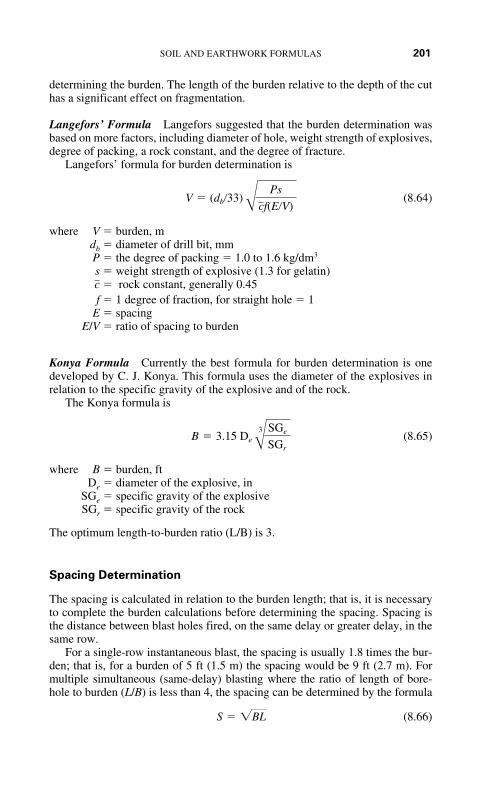
SOIL AND EARTHWORK FORMULAS 201
determining the burden. The length of the burden relative to the depth of the cuthas a significant effect on fragmentation.
Langefors’ Formula Langefors suggested that the burden determination wasbased on more factors, including diameter of hole, weight strength of explosives,degree of packing, a rock constant, and the degree of fracture.
Langefors’ formula for burden determination is
(8.64)
where V � burden, mdb � diameter of drill bit, mmP � the degree of packing � 1.0 to 1.6 kg/dm3
s � weight strength of explosive (1.3 for gelatin)� rock constant, generally 0.45
f � 1 degree of fraction, for straight hole � 1E � spacing
E/V � ratio of spacing to burden
Konya Formula Currently the best formula for burden determination is onedeveloped by C. J. Konya. This formula uses the diameter of the explosives inrelation to the specific gravity of the explosive and of the rock.
The Konya formula is
(8.65)
where B � burden, ftDe � diameter of the explosive, in
SGe � specific gravity of the explosiveSGr � specific gravity of the rock
The optimum length-to-burden ratio (L/B) is 3.
Spacing Determination
The spacing is calculated in relation to the burden length; that is, it is necessaryto complete the burden calculations before determining the spacing. Spacing isthe distance between blast holes fired, on the same delay or greater delay, in thesame row.
For a single-row instantaneous blast, the spacing is usually 1.8 times the bur-den; that is, for a burden of 5 ft (1.5 m) the spacing would be 9 ft (2.7 m). Formultiple simultaneous (same-delay) blasting where the ratio of length of bore-hole to burden (L/B) is less than 4, the spacing can be determined by the formula
(8.66)S � �BL
B � 3.15 DeB3 SGe
SGr
c
V � (db�33)BPs
cf(E�V)

202 CHAPTER EIGHT
where B � burden, ftL � length of borehole, ft
If the length-to-burden ratio is greater than 4, then the spacing is twice theburden. Therefore, if the L/B is 5 the spacing is determined by S = 2B. Forexample, if the burden were equal to 7 ft (2.1 m), the spacing would be
again showing the relationship of the length of borehole to the burden and spac-ing dimensions.
Stemming
There must be some substance put into the top of every borehole to preventthe explosive gases from escaping prematurely. This substance is called“stemming.”
Generally the amount of stemming required will range from 0.7B to 1B.Therefore, in the case of burdens of 8 ft (2.4 m) the stemming will be some-where between 5.6 ft (1.7 m) and 8 ft (2.4 m). That is, the ratio of stemming toburden can vary through this range depending on existing conditions. The con-dition most likely to affect the amount of stemming is the structural integrity ofthe material in the area of the borehole collar. If the material is very competent,as is a homogeneous granite, the stemming will approach 0.7B. However, if thematerial is fractured rock with many fissures and dirt seams, the required ratioof stemming to burden will be approximately 1. In material other than rock,such as overburden, the ratio of stemming to burden will be even greater. Over-burden is generally treated in a 2:1 ratio over rock; that is, 2 ft of overburden isapproximately equal to 1 ft of rock for stemming purposes. Therefore, if thereis 4 ft (1.2 m) of overburden on a shot that requires a burden of 7 ft (2.1 m), thestemming is calculated as follows.
Using the ratio of 0.7B, the stemming would ordinarily be 5 ft (1.5 m).However, with 4 ft (1.2 m) of overburden, for stemming purposes equal to 2 ft(0.6 m) of rock, the actual amount of stemming is 7 ft (2.1 m). Another way ofexpressing it is to compute the required stemming and then add one-half theoverburden depth. Thus
(8.67)
where B � burdenOB � overburden
To compute stemming for a side hill cut, use a right triangle and 2 to 1 ratio,as shown in Fig. 8.2.
Stemming � 0.7B �OB
2
S � 2(7) ft
� 14 ft

SOIL AND EARTHWORK FORMULAS 203
Air Concussion
Air concussion, or air blast, is a pressure wave traveling through the air; it isgenerally not a problem in construction blasting. The type of damage created byair concussion is broken windows. However, it must be realized that a properlyset window glass can generally tolerate pressures of up to 2 lb/in2 (13.8 kN/m2),whereas a wind of 100 mi/h (161 km/h) produces a pressure of only 0.35 lb/in2
(2.4 kN/m2).Air concussion is caused by the movement of a pressure wave generally
caused by one or more of three things: a direct surface energy release, a releaseof inadequately confined gases, and a shock wave from a large free face (seeFig. 8.3). Direct surface energy release is caused by detonation of an explosionon the surface.
Air concussion is also referred to as “overpressure,” that is, the air pressureover and above normal air pressure. The difference between noise and concus-sion is the frequency: air blast frequencies below 20 hertz (Hz), or cycles persecond, are concussions, because they are inaudible to human ears: whereasany air blast above 20 Hz is noise, because it is audible.
Overpressure can be measured in two ways: in pounds of pressure persquare inch (lb/in2) or in decibels (dB). Decibels are a measurement or expres-sion of the relative difference of power of sound waves. Pounds per square inchand decibels can be made relative by the following equation:
(8.68)
where overpressure (dB) � overpressure in decibelslog � the common logarithm
p � overpressure in lb/in2
p0 � 3 � 10–9 lb/in2
overpressure (dB) � 20 log p
p0
Top of explosive column
10
5
2 to 1
Stemming = 10 ft
5
Nearest freeface
FIGURE 8.2 To compute the stemming for a side hill cut, usea right triangle, as shown here. (Hemphill-Blasting operationsMcGraw-Hill.)

204 CHAPTER EIGHT
Vibration Control in Blasting*
Vibrations caused by blasting are propagated with a velocity V, ft/s; frequencyf, Hz; and wavelength L, ft, related by
(8.69)
Velocity v, in/s, of the particles disturbed by the vibrations depends on theamplitude of the vibrations A, in
(8.70)
If the velocity v1 at a distance D1 from the explosion is known, the velocity v2 ata distance D2 from the explosion may be estimated from
(8.71)v2 � v1� D1
D2�
1.5
v � 2 fA
L �V
f
Surface detonation Mudseam
Long free face
Inadequate stemmingof mudseam
FIGURE 8.3 Three causes of air blast. (Hemphill-Blastingoperations, McGraw-Hill.)
*Merritt—Standard Handbook of Civil Engineering, McGraw-Hill.

SOIL AND EARTHWORK FORMULAS 205
The acceleration a, in/s2, of the particles is given by
(8.72)
For a charge exploded on the ground surface, the overpressure P, psi, may becomputed from
(8.73)
where W � maximum weight of explosives, lb per delayD � distance, ft, from explosion to exposure
The sound pressure level, decibels, may be computed from
(8.74)
For vibration control, blasting should be controlled with the scaled-distanceformula:
(8.75)
where � � constant (varies for each site)H � constant (varies for each site)
Distance to exposure, ft, divided by the square root of maximum pounds perdelay is known as scaled distance.
v � H� D
�W ��β
dB � � P
6.95 � 10�28 �0.084
P � 226.62� W1�3
D �1.407
a � 4 2f 2A

This page intentionally left blank

CHAPTER 9
207
BUILDING ANDSTRUCTURESFORMULAS
LOAD-AND-RESISTANCE FACTOR DESIGN FOR SHEAR IN BUILDINGS
Based on the American Institute of Steel Construction (AISC) specifications forload-and-resistance factor design (LRFD) for buildings, the shear capacity Vu,kip (kN � 4.448 � kip), of flexural members may be computed from the fol-lowing:
(9.1)
(9.2)
(9.3)
where Fyw � specified minimum yield stress of web, ksi (MPa � 6.894 � ksi)Aw � web area, in2 (mm2) � dtw
� �
k � 5 if a/h exceeds 3.0 or 67,600/(h/tw)2, or if stiffeners are not required� 5 � 5/(a /h)2, otherwise
Stiffeners are required when the shear exceeds Vu. In unstiffened girders,h/tw may not exceed 260. In girders with stiffeners, maximum h/tw permitted is
for or for , where Fyf
is the specified minimum yield stress, ksi, of the flange. For shear capacity withtension-field action, see the AISC specification for LRFD.
a/h > 1.514,000/�Fyf (Fyf � 16.5)a/h � 1.52,000/�Fyf
1872k /Fyw
Vu �23,760kAw
(h/tw)2 when h
tw
1.25�
Vu �0.54�Fyw Aw
h/tw
when � �h
tw
� 1.25�
Vu � 0.54Fyw Aw when h
tw
� �

208 CHAPTER NINE
ALLOWABLE-STRESS DESIGN FOR BUILDING COLUMNS
The AISC specification for allowable-stress design (ASD) for buildings pro-vides two formulas for computing allowable compressive stress Fa, ksi(MPa), for main members. The formula to use depends on the relationshipof the largest effective slenderness ratio Kl/r of the cross section of anyunbraced segment to a factor Cc defined by the following equation andTable 9.1:
(9.4)
where E � modulus of elasticity of steel� 29,000 ksi (128.99 GPa)
Fy � yield stress of steel, ksi (MPa)
When Kl/r is less than Cc,
(9.5)
where F.S. � safety factor � .
When Kl /r exceeds Cc,
(9.6)
The effective-length factor K, equal to the ratio of effective-column lengthto actual unbraced length, may be greater or less than 1.0. Theoretical K valuesfor six idealized conditions, in which joint rotation and translation are eitherfully realized or nonexistent, are tabulated in Fig. 9.1.
Fa �12 2E
23(Kl/r)2 �150,000
(Kl/r)2
5
3�
3(Kl/r)
8Cc
�(Kl/r)3
8C3c
Fa ��1 �
(Kl/r)2
2C2c� Fy
F.S.
Cc � B2 2E
Fy
�756.6
�Fy
TABLE 9.1 Values of Cc
Fy Cc
36 126.150 107.0

BUILDING AND STRUCTURES FORMULAS 209
LOAD-AND-RESISTANCE FACTOR DESIGN FOR BUILDING COLUMNS
Plastic analysis of prismatic compression members in buildings is permitted ifdoes not exceed 800 and Fu � 65 ksi (448 MPa). For axially loaded
members with b/t � �r, the maximum load Pu, ksi (MPa � 6.894 � ksi), may becomputed from
(9.7)
where Ag � gross cross-sectional area of the memberFcr � 0.658�Fy for � � 2.25
� 0.877 Fy /� for � 2.25� � (Kl /r)2(Fy /286,220)
The AISC specification for LRFD presents formulas for designing memberswith slender elements.
ALLOWABLE-STRESS DESIGN FOR BUILDING BEAMS
The maximum fiber stress in bending for laterally supported beams and girdersis Fb � 0.66Fy if they are compact, except for hybrid girders and members withyield points exceeding 65 ksi (448.1 MPa). Fb � 0.60Fy for noncompact
Pu � 0.85AgFcr
�Fy (l/r)
2.0
2.0
2.0
2.10
1.0
1.0
1.0
1.2
0.7
0.80
0.5
(f)(e)(d)(c)(b)(a)
0.65Recommended design value whenideal conditions are approximated
End condition
Rotation fixed and translation fixed
Rotation fixed and translation free
Rotation free and translation free
Rotation free and translation fixed
Theoretical K value
Buckled shape of columnis shown by dashed line
FIGURE 9.1 Values of effective-length factor K for columns.

210 CHAPTER NINE
sections. Fy is the minimum specified yield strength of the steel, ksi (MPa).Table 9.2 lists values of Fb for two grades of steel.
The allowable extreme-fiber stress of 0.60Fy applies to laterally supported,unsymmetrical members, except channels, and to noncompact box sections.Compression on outer surfaces of channels bent about their major axis shouldnot exceed 0.60Fy or the value given by Eq. (9.12).
The allowable stress of 0.66Fy for compact members should be reduced to0.60Fy when the compression flange is unsupported for a length, in (mm),exceeding the smaller of
(9.8)
(9.9)
where bf � width of compression flange, in (mm) d � beam depth, in (mm)
Af � area of compression flange, in2 (mm2)
The allowable stress should be reduced even more when l/rT exceeds certainlimits, where l is the unbraced length, in (mm), of the compression flange, andrT is the radius of gyration, in (mm), of a portion of the beam consisting of thecompression flange and one-third of the part of the web in compression.
For , use
(9.10)
For , use
(9.11)
where Cb � modifier for moment gradient (Eq. 9.13).
Fb �170,000Cb
(l/rT)2
l/rT �510,000Cb/Fy
Fb � � 2
3�
Fy(l/rT)2
1,530,000Cb� Fy
�102,000Cb/Fy � l/rT � �510,00Cb /Fy
lmax �20,000
Fyd/Af
lmax �76.0bf
�Fy
TABLE 9.2 Allowable Bending Stresses in BracedBeams for Buildings
Yield strength, Compact, Noncompact,ksi (MPa) 0.66Fy (MPa) 0.60Fy (MPa)
36 (248.2) 24 (165.5) 22 (151.7) 50 (344.7) 33 (227.5) 30 (206.8)
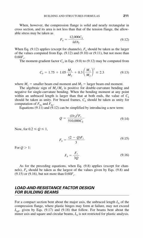
BUILDING AND STRUCTURES FORMULAS 211
When, however, the compression flange is solid and nearly rectangular incross section, and its area is not less than that of the tension flange, the allow-able stress may be taken as
(9.12)
When Eq. (9.12) applies (except for channels), Fb should be taken as the largerof the values computed from Eqs. (9.12) and (9.10) or (9.11), but not more than0.60Fy.
The moment-gradient factor Cb in Eqs. (9.8) to (9.12) may be computed from
(9.13)
where M1 � smaller beam end moment and M2 � larger beam end moment.The algebraic sign of M1 /M2 is positive for double-curvature bending and
negative for single-curvature bending. When the bending moment at any pointwithin an unbraced length is larger than that at both ends, the value of Cbshould be taken as unity. For braced frames, Cb should be taken as unity forcomputation of Fbx and Fby.
Equations (9.11) and (9.12) can be simplified by introducing a new term:
(9.14)
Now, for 0.2 � Q � 1,
(9.15)
For Q 1:
(9.16)
As for the preceding equations, when Eq. (9.8) applies (except for chan-nels), Fb should be taken as the largest of the values given by Eqs. (9.8) and(9.15) or (9.16), but not more than 0.60Fy.
LOAD-AND-RESISTANCE FACTOR DESIGNFOR BUILDING BEAMS
For a compact section bent about the major axis, the unbraced length Lb of thecompression flange, where plastic hinges may form at failure, may not exceedLpd , given by Eqs. (9.17) and (9.18) that follow. For beams bent about theminor axis and square and circular beams, Lb is not restricted for plastic analysis.
Fb �Fy
3Q
Fb �(2 � Q)Fy
3
Q �(l/rT)2Fy
510,000Cb
Cb � 1.75 � 1.05M1
M2� 0.3 � M1
M2�
2
� 2.3
Fb �12,000Cb
ld /Af

212 CHAPTER NINE
For I-shaped beams, symmetrical about both the major and the minor axis orsymmetrical about the minor axis but with the compression flange larger thanthe tension flange, including hybrid girders, loaded in the plane of the web:
(9.17)
where Fyc � minimum yield stress of compression flange, ksi (MPa)M1 � smaller of the moments, in�kip (mm�MPa) at the ends of the
unbraced length of beamMp � plastic moment, in�kip (mm�MPa)ry � radius of gyration, in (mm), about minor axis
The plastic moment Mp equals Fy Z for homogeneous sections, where Z � plas-tic modulus, in3 (mm3); and for hybrid girders, it may be computed from thefully plastic distribution. M1/Mp is positive for beams with reverse curvature.
For solid rectangular bars and symmetrical box beams:
(9.18)
The flexural design strength 0.90Mn is determined by the limit state of lateral-torsional buckling and should be calculated for the region of the last hinge toform and for regions not adjacent to a plastic hinge. The specification gives for-mulas for Mn that depend on the geometry of the section and the bracing pro-vided for the compression flange.
For compact sections bent about the major axis, for example, Mn depends onthe following unbraced lengths:
Lb � the distance, in (mm), between points braced against lateral displace-ment of the compression flange or between points braced to preventtwist
Lp � limiting laterally unbraced length, in (mm), for full plastic-bendingcapacity
� for I shapes and channels
� for solid rectangular bars and box beams
Fyf � flange yield stress, ksi (MPa) J � torsional constant, in4 (mm4) (see AISC “Manual of Steel Construction”
on LRFD)A � cross-sectional area, in2 (mm2)Lr � limiting laterally unbraced length, in (mm), for inelastic lateral buckling
For I-shaped beams symmetrical about the major or the minor axis, or sym-metrical about the minor axis with the compression flange larger than the ten-sion flange and channels loaded in the plane of the web:
(9.19)Lr �ry x1
Fyw � Fr21 � �1 � X2 FL
2
3750(ry /Mp)/�JA
300ry / �Fyf
Lpd �5000 � 3000(M1/Mp)
Fy
ry � 3000ry
Fy
Lpd �3600 � 2200(M1/Mp)
Fycry

BUILDING AND STRUCTURES FORMULAS 213
where Fyw � specified minimum yield stress of web, ksi (MPa)Fr � compressive residual stress in flange
� 10 ksi (68.9 MPa) for rolled shapes, 16.5 ksi (113.6 MPa), forwelded sections
FL � smaller of Fyf � Fr or FywFyf � specified minimum yield stress of flange, ksi (MPa)
X1 �
X2 � (4Cw/Iy) (Sx/GJ)2
E � elastic modulus of the steelG � shear modulus of elasticitySx � section modulus about major axis, in3 (mm3) (with respect to the
compression flange if that flange is larger than the tension flange)Cw � warping constant, in6 (mm6) (see AISC manual on LRFD)Iy � moment of inertia about minor axis, in4 (mm4)
For the previously mentioned shapes, the limiting buckling moment Mr, ksi (MPa),may be computed from
(9.20)
For compact beams with Lb � Lr, bent about the major axis,
(9.21)
where Cb � 1.75 � 1.05(M1 /M2) � 0.3(M1 /M2) � 2.3, where M1 is the smallerand M2 the larger end moment in the unbraced segment of the beam; M1/M2 ispositive for reverse curvature and equals 1.0 for unbraced cantilevers andbeams with moments over much of the unbraced segment equal to or greaterthan the larger of the segment end moments. (See Galambos, T. V., Guide toStability Design Criteria for Metal Structures, 4th ed., John Wiley & Sons, NewYork, for use of larger values of Cb.)
For solid rectangular bars bent about the major axis,
(9.22)
and the limiting buckling moment is given by:
(9.23)
For symmetrical box sections loaded in the plane of symmetry and bent aboutthe major axis, Mr should be determined from Eq. (9.20) and Lr from Eq. (9.22)
For compact beams with Lb > Lr, bent about the major axis,
(9.24)
where Mcr � critical elastic moment, kip�in (MPa�mm).
Mn � Mcr � Cb Mr
Mr � Fy Sx
Lr � 57,000 � ry
Mr� �JA
Mn � Cb �Mp � (Mp � Mr)Lb � Lp
Lr � Lp� � Mp
Mr � FL Sx
( /Sx)2EGJA/2

214 CHAPTER NINE
For shapes to which Eq. (9.24) applies,
(9.25)
For solid rectangular bars and symmetrical box sections,
(9.26)
For determination of the flexural strength of noncompact plate girders andother shapes not covered by the preceding requirements, see the AISC manualon LRFD.
ALLOWABLE-STRESS DESIGN FOR SHEAR IN BUILDINGS
The AISC specification for ASD specifies the following allowable shearstresses Fv, ksi (ksi � 6.894 � MPa):
(9.27)
(9.28)
where Cv � 45,000kv /Fy(h/tw)2 for Cv � 0.8
� for Cv 0.8
kv � 4.00 � 5.34/(a /h)2 for a /h � 1.0� 5.34 � 4.00/(a /h)2 for a /h 1.0
a � clear distance between transverse stiffeners
The allowable shear stress with tension-field action is
(9.29)
When the shear in the web exceeds Fv, stiffeners are required.Within the boundaries of a rigid connection of two or more members with
webs lying in a common plane, shear stresses in the webs generally are high.The commentary on the AISC specification for buildings states that such websshould be reinforced when the calculated shear stresses, such as those along
where Cv � 1,
Fv �Fy
289 �Cv �1 � Cv
1.15√1 � (a/h)2 � � 0.40Fy
236,000kv /Fy(h/tw)2
Fv �Cv Fy
289� 0.40Fy h
tw
380
�Fy
Fv � 0.40Fy h
tw
�380
�Fy
Mcr �57,000Cb �JA
Lb / ry
Mcr � Cb
Lb BEIy GJ � Iy Cw � E
Lb�
2

BUILDING AND STRUCTURES FORMULAS 215
plane AA in Fig. 9.2, exceed Fv, that is, when F is larger than dctwFv, where dcis the depth and tw is the web thickness of the member resisting F. The shearmay be calculated from
(9.30)
where Vs � shear on the sectionM1 � M1L � M1G
M1L � moment due to the gravity load on the leeward side of the connectionM1G � moment due to the lateral load on the leeward side of the connection M2 � M2L � M2G
M2L � moment due to the lateral load on the windward side of theconnection
M2G � moment due to the gravity load on the windward side of theconnection
STRESSES IN THIN SHELLS
Results of membrane and bending theories are expressed in terms of unit forcesand unit moments, acting per unit of length over the thickness of the shell. Tocompute the unit stresses from these forces and moments, usual practice is to
F �M1
0.95d1�
M2
0.95d2� Vs
Lower-story shear
M2
M1
d2
A
dc
d1
ΣFA
Upper-story shear, Vs
FIGURE 9.2 Rigid connection of steel members with websin a common plane.

216 CHAPTER NINE
assume normal forces and shears to be uniformly distributed over the shellthickness and bending stresses to be linearly distributed.
Then, normal stresses can be computed from equations of the form:
(9.31)
where z � distance from middle surfacet � shell thickness
Mx � unit bending moment about an axis parallel to direction of unit nor-mal force Nx
Similarly, shearing stresses produced by central shears T and twisting momentsD may be calculated from equations of the form:
(9.32)
Normal shearing stresses may be computed on the assumption of a parabolicstress distribution over the shell thickness:
(9.33)
where V � unit shear force normal to middle surface.
BEARING PLATES
To resist a beam reaction, the minimum bearing length N in the direction of thebeam span for a bearing plate is determined by equations for prevention oflocal web yielding and web crippling. A larger N is generally desirable but islimited by the available wall thickness.
When the plate covers the full area of a concrete support, the area, in2 (mm2),required by the bearing plate is
(9.34)
where R � beam reaction, kip (kN), fc� � specified compressive strength of theconcrete, ksi (MPa). When the plate covers less than the full area of the con-crete support, then, as determined from Table 9.3
(9.35)
where A2 � full cross-sectional area of concrete support, in2 (mm2).
A1 � � R
0.35 fc� �A2�
2
A1 �R
0.35 f c�
vxz �V
t3/6 � t2
4� z2�
vxy �T
t�
D
t3/12z
fx �Nx
t�
Mx
t 3/12z

BUILDING AND STRUCTURES FORMULAS 217
With N established, usually rounded to full inches (millimeters), the mini-mum width of plate B, in (mm), may be calculated by dividing A1 by N andthen rounded off to full inches (millimeters), so that BN � A1. Actual bearingpressure fp, ksi (MPa), under the plate then is
(9.36)
The plate thickness usually is determined with the assumption of cantileverbending of the plate:
(9.37)
where t � minimum plate thickness, in (mm)k � distance, in (mm), from beam bottom to top of web fillet
Fb � allowable bending stress of plate, ksi (MPa)
COLUMN BASE PLATES
The area A1, in2 (mm2), required for a base plate under a column supported by
concrete should be taken as the larger of the values calculated from the equa-tion cited earlier, with R taken as the total column load, kip (kN), or
(9.38)
Unless the projections of the plate beyond the column are small, the plate maybe designed as a cantilever assumed to be fixed at the edges of a rectangle withsides equal to 0.80b and 0.95d, where b is the column flange width, in (mm), andd is the column depth, in (mm).
A1 �R
0.70 fc�
t � � 1
2B � k�B
3fp
Fb
fp �R
BN
TABLE 9.3 Allowable Bearing Stress, Fp, on Concrete andMasonry*
Full area of concrete support
Less than full area of concretesupport
Sandstone and limestone 0.40
Brick in cement mortar 0.25
*Units in MPa � 6.895 � ksi.
0.35fc�BA1
A2� 0.70fc�
0.35fc�

218 CHAPTER NINE
To minimize material requirements, the plate projections should be nearlyequal. For this purpose, the plate length N, in (mm) (in the direction of d), maybe taken as
(9.39)
The width B, in (mm), of the plate then may be calculated by dividing A1 by N.Both B and N may be selected in full inches (millimeters) so that BN � A1. Inthat case, the bearing pressure fp, ksi (MPa), may be determined from the preced-ing equation. Thickness of plate, determined by cantilever bending, is given by
(9.40)
where Fy � minimum specified yield strength, ksi (MPa), of plate; and p �larger of 0.5(N � 0.95d) and 0.5(B � 0.80b).
When the plate projections are small, the area A2 should be taken as the maxi-mum area of the portion of the supporting surface that is geometrically similar toand concentric with the loaded area. Thus, for an H-shaped column, the columnload may be assumed distributed to the concrete over an H-shaped area with flangethickness L, in (mm), and web thickness 2L:
(9.41)
where Fp � allowable bearing pressure, ksi (MPa), on support. (If L is an imaginarynumber, the loaded portion of the supporting surface may be assumed rectangularas discussed earlier.) Thickness of the base plate should be taken as the larger of thevalues calculated from the preceding equation and
(9.42)
BEARING ON MILLED SURFACES
In building construction, allowable bearing stress for milled surfaces, includingbearing stiffeners, and pins in reamed, drilled, or bored holes, is Fp � 0.90Fy,where Fy is the yield strength of the steel, ksi (MPa).
For expansion rollers and rockers, the allowable bearing stress, kip/linear in(kN/mm), is
(9.43)
where d is the diameter, in (mm), of the roller or rocker. When parts in contacthave different yield strengths, Fy is the smaller value.
Fp �Fy � 13
20 0.66d
t � LB3fp
Fb
L �1
4 (d � b) �
1
4 B(d � b)2 �4R
Fp
t � 2pBfp
Fy
N � �A1 � 0.5(0.95d � 0.80b)

BUILDING AND STRUCTURES FORMULAS 219
PLATE GIRDERS IN BUILDINGS
For greatest resistance to bending, as much of a plate girder cross section aspracticable should be concentrated in the flanges, at the greatest distance fromthe neutral axis. This might require, however, a web so thin that the girderwould fail by web buckling before it reached its bending capacity. To precludethis, the AISC specification limits h/t.
For an unstiffened web, this ratio should not exceed
(9.44)
where Fy � yield strength of compression flange, ksi (MPa).Larger values of h/t may be used, however, if the web is stiffened at appro-
priate intervals.For this purpose, vertical angles may be fastened to the web or vertical plates
welded to it. These transverse stiffeners are not required, though, when h/t is lessthan the value computed from the preceding equation or Table 9.4.
With transverse stiffeners spaced not more than 1.5 times the girder depthapart, the web clear-depth/thickness ratio may be as large as
(9.45)
If, however, the web depth/thickness ratio h/t exceeds , where Fb,ksi (MPa), is the allowable bending stress in the compression flange that wouldordinarily apply, this stress should be reduced to , given by the followingequations:
(9.46)
(9.47)
(9.48)Re � � 12 � (Aw/Af)(3� � �3)
12 � 2(Aw /Af) � � 1.0
RPG � �1 � 0.0005Aw
Af� h
t�
760
�Fb�� � 1.0
Fb� � RPGRe Fb
Fb�
760/ �Fb
h
t�
2000
�Fy
h
t�
14,000
�Fy (Fy � 16.5)
TABLE 9.4 Critical h/t for Plate Girders in Buildings
Fy, ksi (MPa)
36 (248) 322 33350 (345) 243 283
2,000
2Fy
14,000
2Fy(Fy � 16.5)

220 CHAPTER NINE
where Aw � web area, in2 (mm2)Af � area of compression flange, in2 (mm2)� � 0.6Fyw/Fb � 1.0
Fyw � minimum specified yield stress, ksi, (MPa), of web steel
In a hybrid girder, where the flange steel has a higher yield strength than theweb, the preceding equation protects against excessive yielding of the lowerstrength web in the vicinity of the higher strength flanges. For nonhybrid gird-ers, Re � 1.0.
LOAD DISTRIBUTION TO BENTS AND SHEAR WALLS
Provision should be made for all structures to transmit lateral loads, such asthose from wind, earthquakes, and traction and braking of vehicles, to foun-dations and their supports that have high resistance to displacement. For thispurpose, various types of bracing may be used, including struts, tension ties,diaphragms, trusses, and shear walls.
Deflections of Bents and Shear Walls
Horizontal deflections in the planes of bents and shear walls can be computedon the assumption that they act as cantilevers. Deflections of braced bents canbe calculated by the dummy-unit-load method or a matrix method. Deflectionsof rigid frames can be computed by adding the drifts of the stories, as deter-mined by moment distribution or a matrix method.
For a shear wall (Fig. 9.3), the deflection in its plane induced by a load in itsplane is the sum of the flexural deflection as a cantilever and the deflection dueto shear. Thus, for a wall with solid rectangular cross section, the deflection atthe top due to uniform load is
(9.49)
where w � uniform lateral loadH � height of the wallE � modulus of elasticity of the wall materialt � wall thickness
L � length of wall
For a shear wall with a concentrated load P at the top, the deflection at the top is
(9.50)
If the wall is fixed against rotation at the top, however, the deflection is
(9.51)�f �P
Et ��H
L �3
� 3H
L �
�c �4P
Et �� H
L �3
� 0.75H
L �
� �1.5wH
Et �� H
L �3
�H
L �

BUILDING AND STRUCTURES FORMULAS 221
Units used in these equations are those commonly applied in United StatesCustomary System (USCS) and the System International (SI) measurements,that is, kip (kN), lb/in2 (MPa), ft (m), and in (mm).
Where shear walls contain openings, such as those for doors, corridors, or win-dows, computations for deflection and rigidity are more complicated. Approxi-mate methods, however, may be used.
COMBINED AXIAL COMPRESSIONOR TENSION AND BENDING
The AISC specification for allowable stress design for buildings includes threeinteraction formulas for combined axial compression and bending.
When the ratio of computed axial stress to allowable axial stress fu /Faexceeds 0.15, both of the following equations must be satisfied:
(9.52)
(9.53)fa
0.60Fy
�fbx
Fbx�
fby
Fby� 1
fa
Fa
�Cmx fbx
(1 � fa /F�ex)Fbx�
Cmy fby
(1 � fa / F�ey)Fby� 1
Wind bent
Shearwalls
Spandrelbeam
Columns
(a)
(c) (d) (e) (f)
(b)
(g)
FIGURE 9.3 Building frame resists lateral forces with (a) wind bents or (b) shearwalls or a combination of the two. Bents may be braced in any of several ways,including (c) X bracing, (d ) K bracing, (e) inverted V bracing, ( f ) knee bracing, and(g) rigid connections.

222 CHAPTER NINE
When fa /Fa � 0.15, the following equation may be used instead of the preced-ing two:
(9.54)
In the preceding equations, subscripts x and y indicate the axis of bending aboutwhich the stress occurs, and
Fa � axial stress that would be permitted if axial force alone existed, ksi (MPa)
Fb � compressive bending stress that would be permitted if bendingmoment alone existed, ksi (MPa)
� , ksi (MPa); as for Fa, Fb, and 0.6Fy, may beincreased one-third for wind and seismic loads
lb � actual unbraced length in plane of bending, in (mm)
rb � radius of gyration about bending axis, in (mm)
K � effective-length factor in plane of bending
fa � computed axial stress, ksi (MPa)
fb � computed compressive bending stress at point under consideration,ksi (MPa)
Cm � adjustment coefficient
WEBS UNDER CONCENTRATED LOADS
Criteria for Buildings
The AISC specification for ASD for buildings places a limit on compressivestress in webs to prevent local web yielding. For a rolled beam, bearing stiffen-ers are required at a concentrated load if the stress fa, ksi (MPa), at the toe ofthe web fillet exceeds Fa � 0.66Fyw, where Fyw is the minimum specified yieldstress of the web steel, ksi (MPa). In the calculation of the stressed area, theload may be assumed distributed over the distance indicated in Fig. 9.4.
For a concentrated load applied at a distance larger than the depth of thebeam from the end of the beam,
(9.55)
where R � concentrated load of reaction, kip (kN)tw � web thickness, in (mm)N � length of bearing, in (mm), (for end reaction, not less than k)k � distance, in (mm), from outer face of flange to web toe of fillet
For a concentrated load applied close to the beam end,
(9.56)fa �R
tw (N � 2.5k)
fa �R
tw (N � 5k)
Fe�149,000/(Klb /rb)2Fe�
fa
Fa
�fbx
Fbx
�fby
Fby
� 1

BUILDING AND STRUCTURES FORMULAS 223
To prevent web crippling, the AISC specification requires that bearing stiff-eners be provided on webs where concentrated loads occur when the compres-sive force exceeds R, kip (kN), computed from the following:
For a concentrated load applied at a distance from the beam end of at least d/2,where d is the depth of beam,
(9.57)
where tf � flange thickness, in (mm).
For a concentrated load applied closer than d/2 from the beam end,
(9.58)
If stiffeners are provided and extend at least one-half of the web, R need not becomputed.
Another consideration is prevention of sidesway web buckling. The AISCspecification requires bearing stiffeners when the compressive force from a con-centrated load exceeds limits that depend on the relative slenderness of web andflange rwf and whether or not the loaded flange is restrained against rotation:
(9.59)
where l � largest unbraced length, in (mm), along either top or bottom flange atpoint of application of load
bf � flange width, in (mm)dc � web depth clear of fillets � d � 2k
rwf �dc /tw
l / bf
R � 34t2w �1 � 3 � N
d �� tw
tf�
1.5
�2Fyw tf /tw
R � 67.5t2w �1 � 3 � N
d �� tw
tf�
1.5
�2Fyw tf /tw
N
N + 2.5k
N + 5k
N
k
k
Toe of fillet
FIGURE 9.4 For investigating web yielding, stresses are assumed to be distributedover lengths of web indicated at the bearings, where N is the length of bearing plates,and k is the distance from outer surface of beam to the toe of the fillet.

224 CHAPTER NINE
Stiffeners are required if the concentrated load exceeds R, kip (kN), computedfrom
(9.60)
where h � clear distance, in (mm), between flanges, and rwf is less than 2.3when the loaded flange is restrained against rotation. If the loaded flange is notrestrained and rwf is less than 1.7,
(9.61)
R need not be computed for larger values of rwf.
DESIGN OF STIFFENERS UNDER LOADS
AISC requires that fasteners or welds for end connections of beams, girders,and trusses be designed for the combined effect of forces resulting frommoment and shear induced by the rigidity of the connection. When flanges ormoment-connection plates for end connections of beams and girders are weldedto the flange of an I- or H-shape column, a pair of column-web stiffeners havinga combined cross-sectional area Ast not less than that calculated from the follow-ing equations must be provided whenever the calculated value of Ast is positive:
(9.62)
where Fyc � column yield stress, ksi (MPa)Fyst � stiffener yield stress, ksi (MPa)
K � distance, in (mm), between outer face of column flange and web toeof its fillet, if column is rolled shape, or equivalent distance if col-umn is welded shape
Pbf � computed force, kip (kN), delivered by flange of moment-connection plate multiplied by , when computed force is due tolive and dead load only, or by , when computed force is due tolive and dead load in conjunction with wind or earthquake forces
twc � thickness of column web, in (mm)tb � thickness of flange or moment-connection plate delivering concen-
trated force, in (mm)
Notwithstanding the preceding requirements, a stiffener or a pair of stiffen-ers must be provided opposite the beam-compression flange when the column-web depth clear of fillets dc is greater than
(9.63)dc �4100twc
3 �Fyc
Pbf
4�3
5�3
Ast �Pbf � Fyctwc(tb � 5K)
Fyst
R � 0.4r3wf
6800t3w
h
R �6800t3
w
h (1 � 0.4r3
wf)

BUILDING AND STRUCTURES FORMULAS 225
and a pair of stiffeners should be provided opposite the tension flange when thethickness of the column flange tf is less than
(9.64)
Stiffeners required by the preceding equations should comply with the follow-ing additional criteria:
1. The width of each stiffener plus half the thickness of the column web shouldnot be less than one-third the width of the flange or moment-connection platedelivering the concentrated force.
2. The thickness of stiffeners should not be less than tb /2.
3. The weld-joining stiffeners to the column web must be sized to carry the forcein the stiffener caused by unbalanced moments on opposite sides of the column.
FASTENERS IN BUILDINGS
The AISC specification for allowable stresses for buildings specifies allowableunit tension and shear stresses on the cross-sectional area on the unthreadedbody area of bolts and threaded parts. (Generally, rivets should not be used indirect tension.) When wind or seismic loads are combined with gravity loads,the allowable stresses may be increased by one-third.
Most building construction is done with bearing-type connections. Allowablebearing stresses apply to both bearing-type and slip-critical connections. In build-ings, the allowable bearing stress Fp, ksi (MPa), on projected area of fasteners is
(9.65)
where Fu is the tensile strength of the connected part, ksi (MPa). Distance mea-sured in the line of force to the nearest edge of the connected part (end distance)should be at least 1.5d, where d is the fastener diameter. The center-to-centerspacing of fasteners should be at least 3d.
COMPOSITE CONSTRUCTION
In composite construction, steel beams and a concrete slab are connected sothat they act together to resist the load on the beam. The slab, in effect, servesas a cover plate. As a result, a lighter steel section may be used.
Construction in Buildings
There are two basic methods of composite construction.
Method 1 The steel beam is entirely encased in the concrete. Composite actionin this case depends on the steel-concrete bond alone. Because the beam is
Fp � 1.2Fu
tf � 0.4BPbf
Fyc

226 CHAPTER NINE
completely braced laterally, the allowable stress in the flanges is 0.66Fy, whereFy is the yield strength, ksi (MPa), of the steel. Assuming the steel to carry thefull dead load and the composite section to carry the live load, the maximum unitstress, ksi (MPa), in the steel is
(9.66)
where MD � dead-load moment, in�kip (kN�mm)ML � live-load moment, in�kip (kN�mm)Ss � section modulus of steel beam, in3 (mm3)Str � section modulus of transformed composite section, in3 (mm3)
An alternative, shortcut method is permitted by the AISC specification. Itassumes that the steel beam carries both live and dead loads and compensatesfor this by permitting a higher stress in the steel:
(9.67)
Method 2 The steel beam is connected to the concrete slab by shear connectors.Design is based on ultimate load and is independent of the use of temporaryshores to support the steel until the concrete hardens. The maximum stress in thebottom flange is
(9.68)
To obtain the transformed composite section, treat the concrete above theneutral axis as an equivalent steel area by dividing the concrete area by n, theratio of modulus of elasticity of steel to that of the concrete. In determination ofthe transformed section, only a portion of the concrete slab over the beam maybe considered effective in resisting compressive flexural stresses (positive-moment regions). The width of slab on either side of the beam centerline thatmay be considered effective should not exceed any of the following:
1. One-eighth of the beam span between centers of supports
2. Half the distance to the centerline of the adjacent beam
3. The distance from beam centerline to edge of slab (Fig. 9.5)
NUMBER OF CONNECTORS REQUIRED FOR BUILDING CONSTRUCTION
The total number of connectors to resist Vh is computed from Vh /q, where q isthe allowable shear for one connector, kip (kN). Values of q for connectors inbuildings are given in structural design guides.
The required number of shear connectors may be spaced uniformly betweenthe sections of maximum and zero moment. Shear connectors should have at
fs �MD � ML
Str� 0.66Fy
fs �MD � ML
Ss
� 0.76Fy
fs �MD
Ss
�ML
Str� 0.66Fy

BUILDING AND STRUCTURES FORMULAS 227
least 1 in (25.4 mm) of concrete cover in all directions; and unless studs arelocated directly over the web, stud diameters may not exceed 2.5 times thebeam-flange thickness.
With heavy concentrated loads, the uniform spacing of shear connectorsmay not be sufficient between a concentrated load and the nearest point ofzero moment. The number of shear connectors in this region should be at least
(9.69)
where M � moment at concentrated load, ft�kip (kN�m)Mmax � maximum moment in span, ft�kip (kN�m)
N1 � number of shear connectors required between Mmax and zero moment� � Str /Ss or Seff /Ss, as applicable
Seff � effective section modulus for partial composite action, in3 (mm3)
Shear on Connectors
The total horizontal shear to be resisted by the shear connectors in building con-struction is taken as the smaller of the values given by the following two equations:
(9.70)
(9.71)
where Vh � total horizontal shear, kip (kN), between maximum positive momentand each end of steel beams (or between point of maximum posi-tive moment and point of contraflexure in continuous beam)
� specified compressive strength of concrete at 28 days, ksi (MPa)Ac � actual area of effective concrete flange, in2 (mm2)As � area of steel beam, in2 (mm2)
fc�
Vh �As Fy
2
Vh �0.85 fc� Ac
2
N2 �N1[(M�/Mmax) � 1]
� � 1
a
Concreteslab
C ≤ Span C C18
a
≤ a12
FIGURE 9.5 Limitations on effective width of concrete slabin a composite steel-concrete beam.

228 CHAPTER NINE
In continuous composite construction, longitudinal reinforcing steel may beconsidered to act compositely with the steel beam in negative-moment regions.In this case, the total horizontal shear, kip (kN), between an interior support andeach adjacent point of contraflexure should be taken as
(9.72)
where Asr � area of longitudinal reinforcement at support within effective area,in2 (mm2); and Fyr � specified minimum yield stress of longitudinal reinforce-ment, ksi (MPa).
PONDING CONSIDERATIONS IN BUILDINGS
Flat roofs on which water may accumulate may require analysis to ensure thatthey are stable under ponding conditions. A flat roof may be considered stableand an analysis does not need to be made if both of the following two equationsare satisfied:
(9.73)(9.74)
where Cp � 32LsLp4 /107Ip
Cs � 32SLs4 /107Is
Lp � length, ft (m), of primary member or girderLs � length, ft (m), of secondary member or purlinS � spacing, ft (m), of secondary membersIp � moment of inertia of primary member, in4 (mm4)Is � moment of inertia of secondary member, in4 (mm4)Id � moment of inertia of steel deck supported on secondary members,
in4/ft (mm4/m)
For trusses and other open-web members, Is should be decreased 15 percent. Thetotal bending stress due to dead loads, gravity live loads, and ponding should notexceed 0.80Fy, where Fy is the minimum specified yield stress for the steel.
LIGHTWEIGHT STEEL CONSTRUCTION
Lightweight steel construction is popular today for a variety of building compo-nents (floors, roofs, walls. etc.) and for entire buildings.* Such constructiontakes many forms, and a number of different designs of structural members andframing systems have been developed.
Id � 25S4/106
Cp � 0.9Cs � 0.25
Vh �Asr Fyr
2
*From Merritt—Building Construction Handbook, McGraw-Hill. Formulas in this section arebased on the work of F. E. Fahy, who, at the time of their preparation, was Chief Engineer, ProductEngineering, Bethlehem Steel Company.

BUILDING AND STRUCTURES FORMULAS 229
For structural design computations, flat compression elements of cold-formed structural members can be divided into two kinds—stiffened elementsand unstiffened elements. Stiffened compression elements are flat compressionelements; that is, plane compression flanges of flexural members and planewebs and flanges of compression members, of which both edges parallel to thedirection of stress are stiffened by a web, flange, stiffening lip, or the like (AISISpecification for the Design of Light Gage Steel Structural Members). A flatelement stiffened at only one edge parallel to the direction of stress is called anunstiffened element. If the sections shown in Fig. 9.6 are used as compressionmembers, the webs are considered stiffened compression elements.
In order that a compression element may qualify as a stiffened compressionelement, its edge stiffeners should comply with the following:
(9.75)
but not less than 9.2t4.
where w/t � flat-width ratio of stiffened elementImin � minimum allowable moment of inertia of stiffener (of any shape)
about its own centroidal axis parallel to stiffened element
Where the stiffener consists of a simple lip bent at right angles to the stiff-ened element, the required overall depth d of such a lip may be determined withsatisfactory accuracy from the following formula:
(9.76)d � 2.8tB6 � w
t �2
� 144
Imin � 1.83t4B� w
t �2
� 144
w
w t w t
Unstiffenedelement
(a) (b)
t
w
t
Stiffenedelement
Stiffeninglip
FIGURE 9.6 Typical lightweight steel compression elements.(Merritt–Building Construction Handbook, McGraw-Hill.)

230 CHAPTER NINE
but not less than 4.8t. A simple lip should not be used as an edge stiffener forany element having a flat-width ratio greater than 60.
For safe-load determination, that is, in computing effective area and sectionmodulus:
(9.77)
where f � computed unit stress in psi in the element based upon effective width.Equation (9.77) is based on a safety factor of about 1.65 against yield stress
at the outer fiber of the section. For any other safety factor m multiply the right-hand side of Eq. (9.77) by
For deflection determinations, that is, in computing moment of inertia to beused in deflection calculations or other calculations involving stiffness:
(9.78)
For a flat-width ratio w/t greater than 10 but not over 25, the compressivestress should not exceed:
(9.79)
where fb � basic design stress, not to exceed 30,000 psiw � width of elementt � thickness
If fb � 20,000 psi, this formula reduces to
(9.80)
Figure 9.7 shows a number compression elements used in lightweight steel con-struction.
For w/t greater than 25, not over 60, the compressive stress should notexceed fc as given by Eqs. (9.79) and (9.80). For angle struts,
(9.81)
For other sections,
(9.82)
Stiffened Light-gage Elements Subject to Local Bucking Compute sectionproperties based on an effective width of each stiffened compression element(Fig. 9.8). Determine the effective width b by means of Eqs. (9.83) and(9.84).
fc � 20,000 � 282w
t
fc �8,090,000
(w/t)2
fc � 24,700 � 470w
t
fc �5
3fb � 8,640 �
1
15 (fb � 12,950)
w
t
� w
t �lim�
5,160
�f
�1.65/m.
� w
t �lim�
4,020
�f

BUILDING AND STRUCTURES FORMULAS 231
For safe-load determinations, that is, in computing effective area and sectionmodulus
(9.83)
where f � unit stress in psi in the element computed on basis of reduced section,psi (MPa)
w � width of the element, in (mm)t � thickness, in (mm)
b
t�
8,040
�f �1 �2,010
(w/t)�f �
FIGURE 9.7 Typical compression elements used in light-weight steel construction. (Merritt–Building ConstructionHandbook, McGraw-Hill.)

232 CHAPTER NINE
w
t
t
t
t t
(a) (b) (c)
12
b 12
b
12
b2
12
b112
b112
b112
b112
b112
b112
b112
b1
12
b 12
b
w12
b 12
b
w12
b 12
b
w12
b 12
b
w1 w1 w1
w2 w2w2
t t tt
(e) (f)
Columns effective area for computing column factor Qa
(g)
12
b212
b2
12
b2
12
b212
b2
w1
(d)
Beams top flange in compression
12
b 12
bw w
FIGURE 9.8 Effective width of stiffened compression elements. (Merritt–Building Con-struction Handbook, McGraw-Hill.)

BUILDING AND STRUCTURES FORMULAS 233
For deflection determinations, that is, in computing moment of inertia to beused in deflection calculations or in other calculations involving stiffness,
(9.84)
with f, w, and t the same as for Eq. (9.83).
Web Stresses in Light-gage Members The shear on the gross web section inlight-gage cold-formed flexural members is usually limited to two-thirds of thebasic working stress in tension and bending, or
(9.85)
whichever is smaller. In this expression h/t is the ratio of depth to web thick-ness, or of stiffener spacing to web thickness, as for plate-girder construction.Where the web consists of two sheets, as in the case of two channels fastenedback to back to form an I section, each sheet should be considered as a separateweb carrying its share of the shear.
(9.86)
In solving this formula, B should not be assigned any value greater than h.
Pmax(1) � 100t2�980 � 42B
t� 0.22
B
t
h
t� 0.11
h
t �
h h
B
B
Pmax (1)
Pmax (1)
t = web thickness, mm
OveralldepthH
OveralldepthH
h = clear distance between flanges, mmB = length of bearing, mmH = overall depth, mm
Maximum End Reaction or Concentrated Load on End of Cantilever forSingle Unreinforced Web of Light-gage Steel
(Grade C steel, corner radii = thickness of material)
Shear, psi,v �64,000,000
(h/t)2
b
t�
10,320
�f �1 �2,580
(w�t)�f �

234 CHAPTER NINE
(9.87)
NOTE: In solving this formula, B should not be assigned any value greaterthan h.
This formula applies only where the distance x is greater than 1.5h. Other-wise, Eq. (9.86) governs.
(9.88)Pmax(3) � 20,000t2�7.4 � 0.93BB
t �
h
t
t
h
B
B
Pmax (3)
Pmax (3)
t = web thickness (each web sheet), mm
h = clear distance between flanges, mm
Maximum Reactions and Concentrated Loads Bearing on RestrainedWeb of Light-gage Steel
(Grade C steel, corner radii = thickness of material)
Pmax(2) � 100t2�3,050 � 23B
t� 0.09
B
t
h
t� 5
h
t �
X X
X
h h
BB
Pmax (2) Pmax (2)
Pmax (1) Pmax (2)
OveralldepthH
OveralldepthH
t = web thickness, mmh = clear distance between flanges, mmB = length of bearing, mmH = overall depth, mm
Maximum Interior Reaction or Concentrated Load on Single UnreinforcedWeb of Light-gage Steel
(Grade C steel, corner radii = thickness of material)

BUILDING AND STRUCTURES FORMULAS 235
(9.89)
Values of P max (4) apply only where the distance x is greater than 1.5h. Other-wise use P max (3).
The effective length of bearing B for substitution in the above formulasshould not be taken as greater than h.
The column-design formulas recommended by American Iron and SteelInstitute specifications for light-gage cold-formed sections consist of a familyof Johnson parabolas all tangent to a single Euler curve. It can be shown that aninfinite number of such parabolas can be drawn, all having the form
(9.90)
and all tangent to a single Euler curve represented by
(9.91)
In Eqs. (9.90) and (9.91), C and D are constants that depend on the safety factoreccentricity allowance, and end fixity, and fy is the yield point of the material.Observe that fy does not appear in Eq. (9.91). The point of tangency between theequations is always at a P/A value equal to half the initial value (fy /2C).
If a form factor or bucking factor Q is introduced such that
(9.92)
where fcr represents the reduced strength of the section due to the presence of widethin elements that buckle locally at stresses below the yield point of the material,then it is a simple matter to transform Eq. (9.90) into a consistent set of columncurves applicable to any value of Q, all tangent to a single curve of Eq. (9.91):
(9.93)P
A�
fy
CQ �
f 2y
DQ2� L
r �2
Q �fcr
fy
P
A�
D/4C2
(L/r)2
P
A�
fy
C�
f 2y
D � L
r �2
P max(4) � 20,000t2�11.1 � 2.41BB
t �
X
X
t
hh
t
BB
Pmax (4) Pmax (4)
Pmax (4) Pmax (4)
t = web thickness (each web sheet), mm
h = clear distance between flanges, mm

236 CHAPTER NINE
(When the effective-width treatment of stiffened elements is used, Q can bedefined as the ratio between effective area and total area of the cross section,and A in the quantity P/A can mean total area of section.)
Since fcr can never be greater than fy, the value of Q as a form factor orbuckling factor can never exceed 1.0. For any section that does not contain anyelement with a flat-width ratio exceeding that for full effectiveness (w/t � 10for unstiffened elements and for stiffened elements), Q � 1.0 anddisappears from the equation.
Unit Stress for Axially Loaded Cold-formed Members For cold-formed,axially loaded compression members of Grade C steel, the allowable unit stressP/A shall be
For L/r less than
(9.94)
For L/r greater than
(9.95)
(AISI) Specification for the Design of Light Gage Steel Structural Members)
where P � total allowable load, lbA � full, unreduced cross-sectional area of member, sq in (mm2)L � unsupported length of member, in (mm)r � radius of gyration of full, unreduced cross section, in (mm)
Q � a factor determined as follows:a. For members composed entirely of stiffened elements, Q is the
ratio between the effective design area, as determined from theeffective-design widths of such elements, and the full or grossarea of the cross section. The effective design area used in deter-mining Q is to be based on the basic design stress allowed in ten-sion and bending—20,000 psi for Grade C steel.
b. For members composed entirely of unstiffened elements, Q is theratio between the allowable compression stress for the weakestelement of the cross section (the element having the largest flat-width ratio) and the basic design stress.
c. For members composed of both stiffened and unstiffened ele-ments, the factor Q is to be the product of a stress factor Q, com-puted as outlined in b above and an area factor Qa computed asoutlined in a above. However, the stress on which Qa is to be basedshall be that value of the unit stress fc used in computing Qs; andthe effective area to be used in computing Qa shall include the fullarea of all unstiffened elements.
It is recommended that L/r not exceed 200, except that duringconstruction a value of 300 may be allowed.
P
A�
149,000,000
(L/r)2
132/2Q,
P
A� 17,000 � 0.485Q2� L
r �2
132/2Q,
4,020/2f

BUILDING AND STRUCTURES FORMULAS 237
Members subject to both axial compression and bending stresses shall be pro-portioned to meet the requirements of both of the following formulas, as applicable:
(9.96)
and at braced points only
(9.97)
where Fa � maximum axial unit stress in compression permitted by this specifi-cation where axial stress only exists
Fb � maximum bending unit stress in compression permitted by this spec-ification where bending stress only exists
(9.98)
fa � axial unit stress, axial load divided by full cross-sectional area ofmember P/A
f �b � bending unit stress, bending moment divided by section modulus ofmember M/S, noting that for members having stiffened compressionelements, section modulus shall be based on effective design widthsof such elements
l � actual unbraced length in plane of bendingrb � radius of gyration about axis of bending
Cm � 0.85, except as follows:1. When fa /Fa is equal to or less than 0.15, the member selected shall
meet the limitation that is equal to or less than unity.2. For restrained compression members in frames braced against joint
translation but not subject to transverse loading between their sup-ports in the plane of loading, Cm may be taken as 0.6 � 0.4 M1/M2,where M1/M2 is the ratio of smaller to larger moments at the ends ofthe critical unbraced length of the member. M1/M2 is positive whenthe unbraced length is bent in single curvature, negative when it isbent in reverse curvature. (Cm should not be taken at less than 0.4.)
3. For restrained compression members in frames braced against jointtranslation in the plane of loading and subject to transverse loadingbetween their supports (joints) in the plane of loading, a value of Cmmay be taken as 0.85 or may be determined by rational analysis.
Braced Wall Studs A fairly common application of cold-formed shapes—and one that requires special treatment—is as load-bearing wall studs in smalllight-occupancy buildings. Cold-formed steel studs are usually I, channel, orzee sections, to both flanges of which collateral materials are fastened. TheAmerican Iron and Steel Institute Specification for the Design of Light-gage Cold-formed Steel Structural Members permits the strength of studs to be computedon the assumption that they are laterally supported in the plane of the wall.
fa/Fa � f �b/Fb
Fe� �149,000,000
(l/rb)2
fa
0.515Q fy
�f �bFb
� 1
fa
Fa
�Cm f �b
(1�fa /F�c)Fb
� 1

238 CHAPTER NINE
However, the wall material and its attachments to the studs must comply withthe following:
1. Wall sheathing is attached to both faces or flanges of the studs.
2. The spacing in inches of attachments of wall material to each face or flangeof the stud does not exceed a in either:
(9.99)
(9.100)
where L � length of stud, inA � full cross-sectional area of stud, sq inr1 � radius of gyration of full cross section of stud about its axis parallel
to wall, inr2 � radius of gyration of full cross section of stud about its axis perpen-
dicular to wall, ink � combined modulus of elastic support, or spring constant, of one
attachment of wall material to stud and of wall material tributary tothat attachment, lb per in (kPa)
For any steel other than Grade C, having a yield point fy, a computed fromEq. (9.99) should be multiplied by (33,000/fy)
2.For continuous attachment—by an adhesive, for example—a should be
taken as unity in solving Eq. (9.99) for k.One attachment and the wall material tributary to it should be able to exert
on the stud a force in the plane of the wall at least equal to
(9.101)
where I2 � moment of inertia of full cross section of stud about its axis perpen-dicular to wall
P � load on stud
For continuous attachment, a � 1.Values of k and F for any particular combination of stud, wall material, and
attaching means can only be determined by test.A satisfactory value of k can be determined from the expression
(9.102)
where Pult � ultimate loadP0 � initial or zero loadn � number of attachmentsy � average change in length between attachments of each of the stud
pieces from initial load P0 to 0.75 Pult
k �0.75Pult � P0
0.5ny
Fmin �kLP
2,600,000�I2(k/a) � 240P
amax �L
2
r2
r1
amax � 0.22r 2
2
Ak

BUILDING AND STRUCTURES FORMULAS 239
For continuous attachment, use n equal to four times the attached lengthalong each faying surface.
Bolting Light-gage Members Bolting is employed as a common means ofmaking field connections in light-gage steel construction. The AISI Specificationfor the Design of Light-gage Steel Structural Members requires that the distancebetween bolt centers, in line of stress, and the distance from bolt center to edgeof sheet, in line of stress, shall not be less than 11/2 times the bolt diameter nor
(9.103)
where P � load on bolt, lb (N)t � thickness of thinnest connected sheet, in (mm)
fb � basic design stress, psi (MPa)
That specification also recommends a limit of 3.5fb for the bearing stress, and amaximum allowable tension stress on net section of
(9.104)
where d � bolt diameter, in (mm)s � spacing perpendicular to line of stress, in (mm)
CHOOSING THE MOST ECONOMIC STRUCTURAL STEEL*
Structural steel is available in different strengths and grades. So when choosingsteel members for a structure, the designer must compare their relative costbased on cross-sectional areas and prices. For two tension members of the samelength but of different steel strengths, their material-cost ratio C2/C1 is:
(9.105)
where A1 and A2 are the cross-sectional areas and p1 and p2 are the materialprices per unit weight. If the members are designed to carry the same load at astress that is a fixed percentage of the yield point, the cross-sectional areas areinversely proportional to the yield stresses. Therefore, their relative materialcost can be expressed as
(9.106)
where Fy1 and Fy2 are the yield stresses of the two steels. The ratio p2/p1 is therelative price factors. Values of this factor for several steels are given in engi-neering handbooks.*
C2
C1�
Fy1
Fy2
p2
p1
C2
C1�
A2
A1
p2
p1
�0.1 � 3d
s � fb
P
fbt
*Brockenbrough and Merritt, Structural Steel Designer’s Handbook, McGraw-Hill.

240 CHAPTER NINE
Beams The optimal section modulus for an elastically designed I-shaped beamresults when the area of both flanges equals half the total cross-sectional area ofthe member. Assume now two members made of steels having different yieldpoints and designed to carry the same bending moment, each beam beinglaterally braced and proportioned for optimal section modulus. Their relativeweight W2/W1 and relative cost C2/C1 are influenced by the web depth-to-thickness ratio d/t. For example, if the two members have the same d/t values,such as a maximum value imposed by the manufacturing process for rolledbeams, the relationships are
(9.107)
(9.108)
If each of the two members has the maximum d/t value that precludes elasticweb buckling, a condition of interest in designing fabricated plate girders, therelationships are
(9.109)
(9.110)
Relative steel costs and weights are given in engineering handbooks.* In makingthese calculations, the designer must remember that members with the same bend-ing moment must be compared. Further, the relative costs of girders used for longspans, may be considerably different from those for conventional structural steel.
Columns For columns, the relative material cost for two columns of differentsteels carrying the same load1 is:
(9.111)
where Fc1 and Fc2 are the column buckling stresses for the two members. Rela-tive costs for various structural steels are given in Brockenbrough and Merritt,Structural Steel Designer’s Handbook, McGraw-Hill.
STEEL CARBON CONTENT AND WELDABILITY
The chemical composition of steel and its welability are often expressed interms of the carbon equivalent of the structural steel, given by*
C2
C1�
Fc1
Fc2
p2
p1�
Fc1/p1
Fc2/p2
C2
C1�
p2
p1� Fy1
Fy2�
1/2
W2
W1� � Fy1
Fy2�
1/2
C2
C1�
p2
p1� Fy1
Fy2�
2/3
W2
W1� � Fy1
Fy2�
2/3
*Brockenbrough and Merritt, Structural Steel Designer’s Handbook, McGraw-Hill.

BUILDING AND STRUCTURES FORMULAS 241
(9.112)
where C � carbon content, %Mn � manganese content, %Cr � chromium content, %
Mo � molybdenum, %V � vanadium, %
Ni � nickel content, %Cu � copper, %
To prevent underbead cracking, the weld must be cooled at an acceptable rate.A higher carbon equivalent requires a longer cooling rate. Refer to ASTM 6 forfurther requirements.
STATICALLY INDETERMINATE FORCES AND MOMENTS IN BUILDING STRUCTURES*
Shear, moment, and deflection formulas for statically indeterminate forcesin rigid frames as present by Roark have the following notation: W � load,lb (kg); w � unit load, lb/linear in (kg/cm); M is positive when clockwise;V is positive when upward; y is positive when upward. Constrainingmoments, applied couples, loads, and reactions are positive when acting asshown. All forces are in pounds; all moments are in inch-pounds; all deflec-tions and dimensions are in inches. � is in radians and tan � � �. I �moment of inertia of the section of the beam with respect to the neutral axisof the beam, in4 (mm4).
With pinned supports, concentrated load on the horizontal member, Fig. 9.9:
(9.113)
(9.114)
With pinned supports, concentrated load on one vertical member, Fig. 9.10:
(9.115)
(9.116)V �Wa � H2(L1 � L2)
L3
H2 � W
2L13
I1�
2a3
I1�
3ab2
I1�
2L12L3
I3�
2L1L3b
I3�
L1L2L3
I3�
L2L3b
I3
2L13
I2�
2L22L3
I3�
2L1L2L3
I3�
2L13
I1�
2L12L3
I3
V1 �wb � H(L2�L1)
L3
H �1
2W
L1L2b � 2L2L3b � 3L2b2� (b3/L3)(L1 � L2)
L1L2L3 � L12L3 � L2
2L3 � L13 � (I3/I1) � L2
3(I3/I2)
Ceq � C �Mn
6�
(Cr � Mo � V)
5�
(Ni � Cu)
15
*Roark—Formulas for Stress and Strain, McGraw-Hill.

242 CHAPTER NINE
With pinned supports and a uniform load on the horizontal member, Fig. 9.11:
(9.117)
(9.118)
With pinned supports and a uniform load on the vertical member, Fig. 9.12:
(9.119)
(9.120)V �12WL1 � H2(L1 � L2)
L3
H2 �1
8W
5L31(I3/I1) � 2L1L2L3 � 4L2
1L3
L31 � (I3/I1) � L3
2(I3/I2) � L21L3 � L2
2L3 � L1L2L3
V1 �12WL3 � H(L1 � L2)
L3
H � WL3
2(L1 � L2)
8L12L3 � 4L1L2L3 � 8L3
1(I3/I1) � 8L32(I3/I2) � 8L2
2L3 � 4L1L2L3
3
12
wba
V1
V2
H
H
3
1 2
wb
a
V
V
H2
H1
FIGURE 9.9 Pinned supports, con-centrated load on the horizontalmember. (Roark–Formulas forStress and Stress, McGraw-Hill.)
FIGURE 9.10 Pinned supports, con-centrated load on one vertical member.(Roark–Formulas for Stress and Strain,McGraw-Hill.)
FIGURE 9.11 Pinned supports,uniform load on horizontal member.(Roark–Formulas for Stress andStrain, McGraw-Hill.)
FIGURE 9.12 Pinned supports, uni-form load on vertical member.(Roark–Formulas for Stress and Strain,McGraw-Hill.)
3
12
W
V1
V2
H
H
3
12W
V
V
H2
H1

BUILDING AND STRUCTURES FORMULAS 243
With fixed supports and a concentrated load on the horizontal member,Fig. 9.13:
(9.121)
(9.122)
(9.123)
With fixed supports and and a concentrated load on one vertical member,Fig. 9.14:
(9.124)
(9.125)
(9.126)
With fixed supports and a uniform load on the horizontal member, Fig. 9.15:
(9.127)
(9.128)
(9.129)12HL2
2
I2�
M2L2
I2�
13M2L3
I3�
16M1L3
I3�
124WL2
3
I3
�12HL2
1
I1�
M1L1
I1�
�13M1L3
I3�
16M2L3
I3�
124WL2
3
I3
12M1L2
1
I1�
13HL3
1
I1�
13HL3
2
I2�
12M2L2
2
I2
12HL2
2
I2�
M2L2
I2�
13M2L3
I3�
16M1L3
I3
12Wa2
I1�
12H2L2
1
I1�
M1L1
I1�
13M1L3
I3�
16M2L3
I3
13Wa3
I1�
12Wa2b
I1�
13H2L3
1
I1�
12M1L2
1
I1�
13H2L3
2
I2�
12M2L2
2
I2
12HL2
2
I2�
M2L2
I2�
13M2L3
I3�
16M1L3
I3�
16W[2bL3 � (b3/L3) � 3b2]
I3
�12HL2
1
I1�
M1L1
I1� �
13M1L3
I3�
16W(bL3 � b3/L3)
I3�
16M2L3
I3
�13HL3
1
I1�
12M1L
21
I1�
13HL3
2
I2�
12M2L
22
I2
FIGURE 9.13 Fixed supports, con-centrated load on horizontal member.(Roark–Formulas for Stress andStrain, McGraw-Hill.)
FIGURE 9.14 Fixed supports, concen-trated load on one vertical member.(Roark–Formulas for Stress and Strain,McGraw-Hill.)
3
1 2
Wba
V1
M1 M2
HV2
H
3
12
Wb
a
V
V
H2
H1
M1 M2

244 CHAPTER NINE
With fixed supports and a uniform load on the vertical member, Fig. 9.16:
(9.130)
(9.131)
(9.132)
ROOF LIVE LOADS*
Some building codes specify that design of flat, curved, or pitched roofs shouldtake into account the effects of occupancy and rain loads and be designed forminimum live loads. Other codes require that structural members in flat,pitched, or curved roofs be designed for a live load Lr (lb per ft2 of horizontalprojection) computed from
(9.133)
where R1 � reduction factor for size of tributary area� 1 for
� 1.2 � 0.001At for 200 < At < 600� 0.6 for At � 600
Al � tributary area, or area contributing load to the structural member, ft2
R2 � reduction factor for slope of roof� 1 for F � 4� 0.6 for F � 12
F � rate of rise for a pitched roof, in/ft� rise-to-span ratio multiplied by 32 for an arch or dome
At � 200
Lr � 20R1R2 � 12
12H2L2
2
I2�
M2L2
I2�
13M2L3
I3�
16M1L3
I3
16WL2
1
I1�
12H2L2
1
I1�
M1L1
I1�
13M1L3
I3�
16M2L3
I3
18WL3
1
I1�
12M1L2
1
I1�
13H2L3
1
I1�
13H2L3
2
I2�
12M2L2
2
I2
3
1 2
W
V1
V2
H
H
M1 M2W
3
12
V
V
H2
H1
M1 M2
FIGURE 9.15 Fixed supports,uniform load on horizontal member.(Roark–Formulas for Stress andStrain, McGraw-Hill.)
FIGURE 9.16 Fixed supports, uni-form load on one vertical member.(Roark–Formulas for Stress and Strain,McGraw-Hill.)
*Brokenbrough and Merritt—Structural Steel Designer’s Handbook, McGraw-Hill.

BUILDING AND STRUCTURES FORMULAS 245
Snow Loads
Determination of designing snow loads for roofs is often based on the maxi-mum ground snow load in 50-year mean recurrence period (2% probability ofbeing exceeded in any year). This load or data for computing it from anextreme-value statistical analysis of weather records of snow on the groundmay be obtained from the local building code or the National Weather Service.
Some building codes and ASCE 7-95 specify an equation that takes intoaccount the consequences of a structural failure in view of the end use of thebuilding to be constructed and the wind exposure of the roof:
(9.134)
where Ce � wind exposure factor (range 0.8 to 1.3)Ct � thermal effects factor (range 1.0 to 1.2)
I � importance factor for end use (range 0.8 to 1.2)pf � roof snow load, lb per ft2
pg � ground snow load for 50-year recurrence period, lb per ft2
The “Low-Rise Building systems Manual,” Metal Building ManufacturersAssociation, Cleveland, Ohio, based on a modified form of ASCE 7, recom-mends that the design of roof snow load be determined from
(9.135)
where Is is an importance factor and C reflects the roof type.
Wind Loads
Wind loads are randomly applied dynamic loads. The intensity of the windpressure on the surface of a structure depends on wind velocity, air density, ori-entation of the structure, area of contact surface, and shape of the structure.Because of the complexity involved in defining both the dynamic wind loadand the behavior of an indeterminate steel structure when subjected to windloads, the design criteria adopted by building codes and standards have beenbased on the application of an equivalent static wind pressure. This equivalentstatic design wind pressure p (psf) is defined in a general sense by
(9.136)
where q � velocity pressure, psfG � gust response factor to account for fluctuations in wind speed
Cp � pressure coefficient or shape factor that reflects the influence of thewind on the various parts of a structure
Velocity pressure is computed from
(9.137)qz � 0.00256 KzKztKdV2I
p � qGCp
pf � IsCpg
pf � 0.7CeCtIpg

246 CHAPTER NINE
where Kz � velocity exposure coefficient evaluated at height zKzt � topographic factorKd � wind directionality factor
I � importance factorV � basic wind speed corresponding to a 3-s gust speed at 33 ft above
the ground in exposure C
Velocity pressures due to wind to be used in building design vary with typeof terrain, distance above ground level, importance of building, likelihood ofhurricanes, and basic wind speed recorded near the building site. The windpressures are assumed to act horizontally on the building area projected on avertical plane normal to the wind direction.
ASCE 7 permits the use of either Method I or Method II to define the designwind loads. Method I is a simplified procedure and may be used for enclosed orpartially enclosed buildings.
ASCE 7 Method II is a rigorous computation procedure that accounts for theexternal, and internal pressure variation as well as gust effects. The following isthe general equation for computing the design wind pressure, p:
(9.138)
where q and qi � velocity pressure as given by ASCE 7G � gust effect factor as given by ASCE 7
Cp � external pressure coefficient as given by ASCE 7GCpt � internal pressure coefficient as given by ASCE 7
Codes and standards may present the gust factors and pressure coefficientsin different formats. Coefficients from different codes and standards should notbe mixed.
Seismic Loads
The engineering approach to seismic design differs from that for other load types.For live, wind or snow loads, the intent of a structural design is to preclude struc-tural damage. However, to achieve an economical seismic design, codes and stan-dards permit local yielding of a structure during a major earthquake. Local yield-ing absorbs energy but results in permanent deformations of structures. Thusseismic design incorporates not only application of anticipated seismic forces butalso use of structural details that ensure adequate ductility to absorb the seismicforces without compromising the stability of structures. Provisions for this areincluded in the AISC specifications for structural steel for buildings.
The forces transmitted by an earthquake to a structure result from vibratoryexcitation of the ground. The vibration has both vertical and horizontal compo-nents. However, it is customary for building design to neglect the vertical com-ponent because most structures have reserve strength in the vertical directiondue to gravity-load design requirements.
Seismic requirements in building codes and standards attempt to translatethe complicated dynamic phenomenon of earthquake force into a simplifiedequivalent static force to be applied to a structure for design purposes. For
p � qGCp � qi(GCpt)

BUILDING AND STRUCTURES FORMULAS 247
example, ASCE 7-95 stipulates that the total lateral force, or base shear, V(kips) acting in the direction of each of the principal axes of the main structuralsystem should be computed from
(9.139)
where Cs � seismic response coefficientW � total dead load and applicable portions of other loads
The seismic coefficient, Cs, is determined by the following equation:
(9.140)
where Cv � seismic coefficient for acceleration dependent (short period) struc-tures
R � response modification factorT � fundamental period, s
Alternatively, Cs need not be greater than
(9.141)
where Ca � seismic coefficient for velocity dependent (intermediate and longperiod) structures.
A rigorous evaluation of the fundamental elastic period, T, requires consid-eration of the intensity of loading and the response of the structure to the load-ing. To expedite design computations, T may be determined by the following:
(9.142)
where CT � 0.035 for steel framesCT � 0.030 for reinforced concrete framesCT � 0.030 steel eccentrically braced framesCT � 0.020 all other buildingshn � height above the basic to the highest level of the building, ft
For vertical distribution of seismic forces, the lateral force, V, should be dis-tributed over the height of the structure as concentrated loads at each floor levelor story. The lateral seismic force, Fx, at any floor level is determined by thefollowing equation:
(9.143)
where the vertical distribution factor is given by
(9.144)
where wx and wi � height from the base to level x or ik � 1 for building having period of 0.5 s or less
� 2 for building having period of 2.5 s or more� use linear interpolation for building periods between 0.5 and 2.5 s
Cux �wxh
kx
ni�1wihk
i
Fx � CuxV
Ta � CT hn3/4
Cs � 2.5Ca/R
Cs � 1.2Cv /RT2/3
V � CsW

248 CHAPTER NINE
For horizontal shear distribution, the seismic design story shear in any story,Vx, is determined by the following:
(9.145)
where Fi � the portion of the seismic base shear induced at level i. The seismicdesign story shear is to be distributed to the various elements of the force-resisting system in a story based on the relative lateral stiffness of the verticalresisting elements and the diaphragm.
Provision also should be made in design of structural framing for horizontaltorsion, overturning effects, and the building drift.
Vx � ni�1Fi

CHAPTER 10
249
BRIDGE ANDSUSPENSION-
CABLE FORMULAS
SHEAR STRENGTH DESIGN FOR BRIDGES
Based on the American Association of State Highway and Transportation Offi-cials (AASHTO) specifications for load-factor design (LFD), the shear capacity,kip (kN), may be computed from
(10.1)
for flexural members with unstiffened webs with h / tw � 150 or for girders withstiffened webs but a/h exceeding 3 or 67,600(h / tw)2:
For girders with transverse stiffeners and a /h less than 3 and 67,600(h / tw)2, theshear capacity is given by
(10.2)
Stiffeners are required when the shear exceeds Vu.Refer to Chap. 9, “Building and Structures Formulas,” for symbols used in
the preceding equations.
Vu � 0.58Fy dtw �C �1 � C
1.15 �1 � (a/h)2 �
�45,000k
Fy (h/tw)2 when h
tw
1.25�
��
h/tw
when � �h
tw
� 1.25�
C � 1.0 when h
tw
� �
Vu � 0.58Fy htwC

250 CHAPTER TEN
ALLOWABLE-STRESS DESIGN FOR BRIDGE COLUMNS
In the AASHTO bridge-design specifications, allowable stresses in concentri-cally loaded columns are determined from the following equations:
When Kl /r is less than Cc,
(10.3)
When Kl /r is equal to or greater than Cc,
(10.4)
See Table 10.1.
LOAD-AND-RESISTANCE FACTOR DESIGN FOR BRIDGE COLUMNS
Compression members designed by LFD should have a maximum strength, kip(kN),
(10.5)
where As � gross effective area of column cross section, in2 (mm2).
For
(10.6)
For
(10.7)Fcr � 2E
(KLc /r)2 �286,220
(KLc /r)2
KLc/r 22 2E/Fy ,
Fcr � Fy �1 �Fy
4 2E � KLc
r �2
�KLc /r � 22 2E/Fy ,
Pu � 0.85As Fcr
Fa � 2E
2.12(Kl/r)2 �135,000
(Kl/r)2
Fa �Fy
2.12 �1 �(Kl/r)2
2C2c�
TABLE 10.1 Column Formulas for Bridge Design
YieldAllowable stress, ksi (MPa)strength,
ksi (MPa) Cc Kl/r � Cc Kl/r � Cc
36 (248) 126.1 16.98–0.00053(Kl/r)2
50 (345) 107.0 23.58–0.00103(Kl/r)2
90 (620) 79.8 42.45–0.00333(Kl/r)2
100 (689) 75.7 47.17–0.00412(Kl/r)2
135,000
(Kl/r)2

BRIDGE AND SUSPENSION-CABLE FORMULAS 251
where Fcr � buckling stress, ksi (MPa)Fy � yield strength of the steel, ksi (MPa)K � effective-length factor in plane of bucklingLc � length of member between supports, in (mm)r � radius of gyration in plane of buckling, in (mm)E � modulus of elasticity of the steel, ksi (MPa)
The preceding equations can be simplified by introducing a Q factor:
(10.8)
Then, the preceding equations can be rewritten as shown next:For Q � 1.0,
(10.9)
For Q 1.0,
(10.10)
ADDITIONAL BRIDGE COLUMN FORMULAS*
The nomenclature for the bridge column formulas is shown at the end of theirexplanation of their applications. For bridges using structural carbon steel withsy � 33,000 psi for the tensile yield strength, or for structural shapes havingtheir ends riveted, the following formulas apply, using the nomenclature givenbelow for formulas from Eqs. (10.11) through (10.33) are known as the ‘secantformula’ when the ‘sec’ expression appears in their denominator:
Q � allowable load, 1b
P � ultimate load, 1b
A � section area of column, sq in
L � length of column, in
r � least radius of gyration of column section, in
Su � ultimate strength, psi
Sy � yield point or yield strength of material, psi
Fcr �Fy
2Q
Fcr � �1 �Q
2 � Fy
Q � � KLc
r �2
� Fy
2 2E �
*Roark—Formulas for Stress and Strain, McGraw-Hill.

252 CHAPTER TEN
E � modulus of elasticity of material, psi
m � factor of safety
(L/r)� � critical slenderness ratio
(10.11)
Suggested Sy � 32,000; suggested m � 1.7
(10.12)
or
(10.13)
(10.14)
(10.15)
When the column ends are pinned, the following formulas apply:
(10.16)
(10.17)
(10.18)
(10.19)
For structural silicon steel with Su � 80,000 psi and Sy � 45,000 psi, usingstructural shapes, or being fabricated with the ends riveted,
(10.20)Q
A� 20,000 � 0.46� L
r �2 up to L
r� 130
P
A� 25,600 � 0.566� L
r �2 up to L
r� 140
P
A�
Sy
1 � 0.25 sec� 0.85L
2r BP
EA �
Q
A�
18,750
1 � 0.25 sec� 0.875L
2r B1.76Q
EA � for L
r 140
Q
A� 15,000 �
1
3 � L
r �2 up to L
r� 140
Q
A�
18,750
1 � 0.25 sec0.75L
2r B1.76Q
EA
for L
r 140
Q
A� 15,000 �
1
4 � L
r �2
up to L
r� 140
P
A� 25,600 � 0.425� L
r �2
up to L
r� 160
P
A�
Sy
1 � 0.25 sec� 0.75L
2 BP
EA �
Q
A�
Sy/m
1 � 0.25 sec� 0.75L
2r BmQ
EA �

BRIDGE AND SUSPENSION-CABLE FORMULAS 253
(10.21)
(10.22)
(10.23)
When the column ends are pinned,
(10.24)
(10.25)
(10.26)
For structural nickel steel with Sy � 55,000 psi, using structural shapes, orbeing fabricated with column ends being riveted,
(10.27)
(10.28)
(10.29)
(10.30)
When the column ends are pinned,
(10.31)
(10.32)
(10.33)P
A� 1.83� Q
A �
Q
A�
30,000
1 � 0.25 sec� 0.875L
2r B1.83Q
EA � for L
r 120
Q
A� 24,000 � 0.86� L
r �2 up to L
r� 120
Q
A� 24,000 � 98� L
r �
P
A� 1.83� Q
A �
Q
A�
30,000
1 � 0.25 sec� 0.75L
2r B1.83Q
EA � for L
r 120
Q
A� 24,000 � 0.66� L
r �2 up to L
r� 120
P
A� 1.8� Q
A �
Q
A�
25,000
1 � 0.25 sec� 0.875L
2r B1.8Q
EA � for L
r 130
Q
A� 20,000 � 0.61� L
r �2 up to L
r� 130
P
A� 1.8� Q
A �
Q
A� 27,000 � 80� L
r � maxQ
A� 23,000
Q
A�
25,000
1 � 0.25 sec� 0.75L
2r B1.8Q
EA � for L
r 130

254 CHAPTER TEN
ALLOWABLE-STRESS DESIGN FOR BRIDGE BEAMS
AASHTO gives the allowable unit (tensile) stress in bending as Fb � 0.55Fy. Thesame stress is permitted for compression when the compression flange is support-ed laterally for its full length by embedment in concrete or by other means.
When the compression flange is partly supported or unsupported in a bridge,the allowable bending stress, ksi (MPa), is (Table 10.2):
(10.34)
where L � length, in (mm), of unsupported flange between connections of lat-eral supports, including knee braces
Sxc � section modulus, in3 (mm3), with respect to the compression flangeIyc � moment of inertia, in4 (mm4) of the compression flange about the
vertical axis in the plane of the webJ � 1/3(bc t3
c � btt3c � Dt3
w)bc � width, in (mm), of compression flangebt � width, in (mm), of tension flangetc � thickness, in (mm), of compression flangett � thickness, in (mm), of tension flange
tw � thickness, in (mm), of webD � depth, in (mm), of webd � depth, in (mm), of flexural member
In general, the moment-gradient factor Cb may be computed from the nextequation. It should be taken as unity, however, for unbraced cantilevers andmembers in which the moment within a significant portion of the unbracedlength is equal to, or greater than, the larger of the segment end moments. Ifcover plates are used, the allowable static stress at the point of cutoff should becomputed from the preceding equation.
The moment-gradient factor may be computed from
(10.35)Cb � 1.75 � 1.05 � M1
M2� � 0.3 � M1
M2�
2
� 2.3
� B0.772J
Iyc� 9.87 � d
L �2
� 0.55Fy
Fb � � 5 � 107Cb
Sxc� � Iyc
L �
TABLE 10.2 Allowable BendingStress in Braced Bridge Beams*
Fy Fb
36 (248) 20 (138)50 (345) 27 (186)
*Units in ksi (MPa).
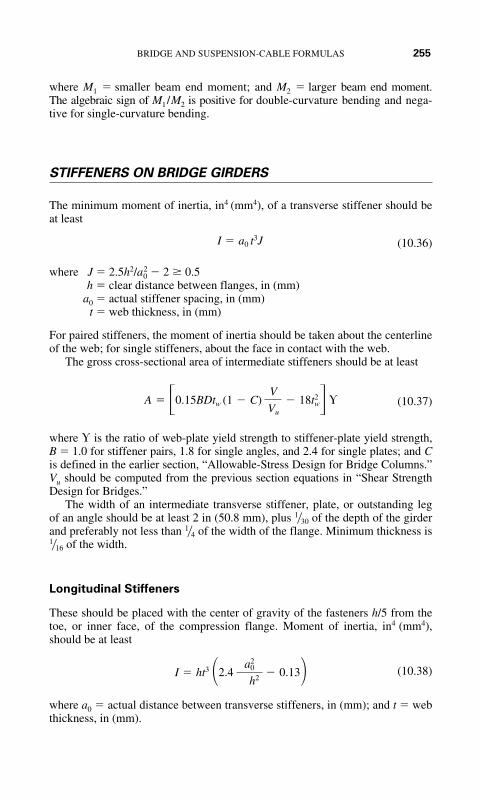
BRIDGE AND SUSPENSION-CABLE FORMULAS 255
where M1 � smaller beam end moment; and M2 � larger beam end moment.The algebraic sign of M1/M2 is positive for double-curvature bending and nega-tive for single-curvature bending.
STIFFENERS ON BRIDGE GIRDERS
The minimum moment of inertia, in4 (mm4), of a transverse stiffener should beat least
(10.36)
where J � 2.5h2/a20 � 2 � 0.5
h � clear distance between flanges, in (mm)a0 � actual stiffener spacing, in (mm)
t � web thickness, in (mm)
For paired stiffeners, the moment of inertia should be taken about the centerlineof the web; for single stiffeners, about the face in contact with the web.
The gross cross-sectional area of intermediate stiffeners should be at least
(10.37)
where " is the ratio of web-plate yield strength to stiffener-plate yield strength,B � 1.0 for stiffener pairs, 1.8 for single angles, and 2.4 for single plates; and Cis defined in the earlier section, “Allowable-Stress Design for Bridge Columns.”Vu should be computed from the previous section equations in “Shear StrengthDesign for Bridges.”
The width of an intermediate transverse stiffener, plate, or outstanding legof an angle should be at least 2 in (50.8 mm), plus of the depth of the girderand preferably not less than of the width of the flange. Minimum thickness is
of the width.
Longitudinal Stiffeners
These should be placed with the center of gravity of the fasteners h/5 from thetoe, or inner face, of the compression flange. Moment of inertia, in4 (mm4),should be at least
(10.38)
where a0 � actual distance between transverse stiffeners, in (mm); and t � webthickness, in (mm).
I � ht3 �2.4a2
0
h2 � 0.13�
1�16
1�4
1�30
A � �0.15BDtw (1 � C)V
Vu
� 18t2w� "
I � a0 t3J

256 CHAPTER TEN
Thickness of stiffener, in (mm), should be at least where b is the stiff-ener width, in (mm); and fb is the flange compressive bending stress, ksi (MPa).The bending stress in the stiffener should not exceed that allowable for the material.
HYBRID BRIDGE GIRDERS
These may have flanges with larger yield strength than the web and may becomposite or noncomposite with a concrete slab, or they may utilize anorthotropic-plate deck as the top flange.
Computation of bending stresses and allowable stresses is generally thesame as that for girders with uniform yield strength. The bending stress in theweb, however, may exceed the allowable bending stress if the computed flangebending stress does not exceed the allowable stress multiplied by
(10.39)
where � � ratio of web yield strength to flange yield strength# � distance from outer edge of tension flange or bottom flange of
orthotropic deck to neutral axis divided by depth of steel section� � ratio of web area to area of tension flange or bottom flange of
orthotropic-plate bridge
LOAD-FACTOR DESIGN FOR BRIDGE BEAMS
For LFD of symmetrical beams, there are three general types of members toconsider: compact, braced noncompact, and unbraced sections. The maximumstrength of each (moment, in�kip) (mm�kN) depends on member dimensionsand unbraced length, as well as on applied shear and axial load (Table 10.3).
The maximum strengths given by the formulas in Table 10.3 apply onlywhen the maximum axial stress does not exceed 0.15Fy A, where A is thearea of the member. Symbols used in Table 10.3 are defined as follows:
Fy � steel yield strength, ksi (MPa)
Z � plastic section modulus, in3 (mm3)
S � section modulus, in3 (mm3)
b� � width of projection of flange, in (mm)
d � depth of section, in (mm)
h � unsupported distance between flanges, in (mm)
M1 � smaller moment, in�kip (mm�kN), at ends of unbraced length of member
Mu � Fy Z
M1 /Mu is positive for single-curvature bending.
R � 1 ��#(1 � �)2 (3 � # � #�)
6 � �#(3 � #)
b�fb /71.2,
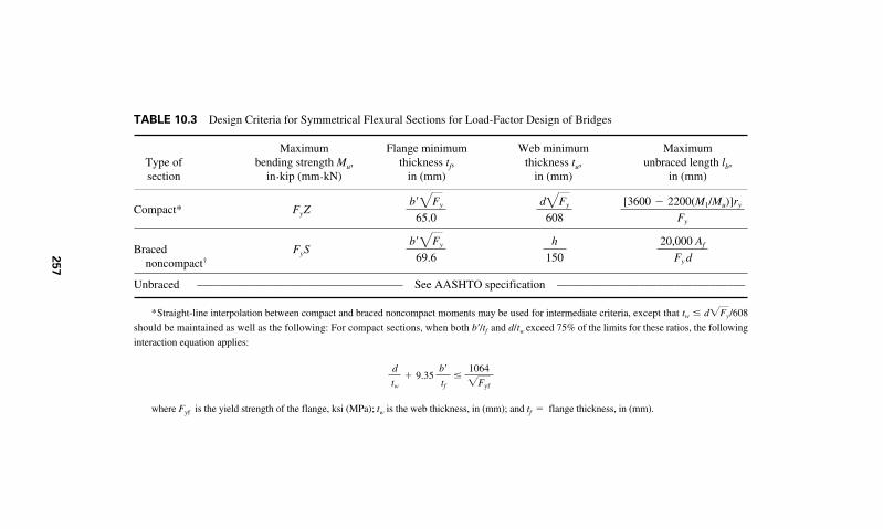
TABLE 10.3 Design Criteria for Symmetrical Flexural Sections for Load-Factor Design of Bridges
Maximum Flange minimum Web minimum Maximum Type of bending strength Mu, thickness tf, thickness tu, unbraced length lb,section in�kip (mm�kN) in (mm) in (mm) in (mm)
Compact* FyZ
Braced FySnoncompact†
Unbraced ___________________________________ See AASHTO specification ________________________________
*Straight-line interpolation between compact and braced noncompact moments may be used for intermediate criteria, except that
should be maintained as well as the following: For compact sections, when both and d/tw exceed 75% of the limits for these ratios, the following
interaction equation applies:
where Fyf is the yield strength of the flange, ksi (MPa); tw is the web thickness, in (mm); and tf � flange thickness, in (mm).
d
tw
� 9.35b�
tf
�1064
�Fyf
b�/tf
tw � d�Fy/608
20,000 Af
Fy d
h
150
b�2Fy
69.6
[3600 � 2200(M1/Mu)]ry
Fy
d2Fy
608
b�2Fy
65.0
257

258 CHAPTER TEN
BEARING ON MILLED SURFACES
For highway design, AASHTO limits the allowable bearing stress on milledstiffeners and other steel parts in contact to Fp � 0.80Fu. Allowable bearingstresses on pins are given in Table 10.4.
The allowable bearing stress for expansion rollers and rockers used inbridges depends on the yield point in tension Fy of the steel in the roller or thebase, whichever is smaller. For diameters up to 25 in (635 mm) the allowablestress, kip/linear in (kN/mm), is
(10.40)
For diameters from 25 to 125 in (635 to 3175 mm),
(10.41)
where d � diameter of roller or rocker, in (mm).
BRIDGE FASTENERS
For bridges, AASHTO specifies the working stresses for bolts. Bearing-typeconnections with high-strength bolts are limited to members in compressionand secondary members. The allowable bearing stress is
(10.42)
where Fp � allowable bearing stress, ksi (MPa); and Fu � tensile strength ofthe connected part, ksi (MPa) (or as limited by allowable bearing on the fas-teners). The allowable bearing stress on A307 bolts is 20 ksi (137.8 MPa) andon structural-steel rivets is 40 ksi (275.6 MPa).
Fp � 1.35Fu
p �Fy � 13
20 3�d
p �Fy � 13
20 0.6d
TABLE 10.4 Allowable Bearing Stresses on Pins*
Bridges
Pins subject Pins not subject Buildings to rotation to rotation
Fy Fp � 0.90Fy Fp � 0.40Fy Fp � 0.80Fy
36 (248) 33 (227) 14 (96) 29 (199)50 (344) 45 (310) 20 (137) 40 (225)
*Units in ksi (MPa).

BRIDGE AND SUSPENSION-CABLE FORMULAS 259
COMPOSITE CONSTRUCTION IN HIGHWAY BRIDGES
Shear connectors between a steel girder and a concrete slab in compositeconstruction in a highway bridge should be capable of resisting both hori-zontal and vertical movement between the concrete and steel. Maximumspacing for shear connectors generally is 24 in (609.6 mm), but wider spacingmay be used over interior supports, to avoid highly stressed portions of thetension flange (Fig. 10.1). Clear depth of concrete cover over shear connec-tors should be at least 2 in (50.8 mm), and they should extend at least 2 in(50.8 mm) above the bottom of the slab.
Span/Depth Ratios
In bridges, for composite beams, preferably the ratio of span/steel beam depthshould not exceed 30 and the ratio of span/depth of steel beam plus slab shouldnot exceed 25.
Effective Width of Slabs
For a composite interior girder, the effective width assumed for the concreteflange should not exceed any of the following:
1. One-fourth the beam span between centers of supports
2. Distance between centerlines of adjacent girders
3. Twelve times the least thickness of the slab
For a girder with the slab on only one side, the effective width of slab shouldnot exceed any of the following:
1. One-twelfth the beam span between centers of supports
2. Half the distance to the centerline of the adjacent girder
3. Six times the least thickness of the slab
Full penetration butt weld
Shear connectorspacing
Half space
C Bearing
Studs
1" Min clearance
2" Min
3"Min24"
Max24"Max 2"MinL
FIGURE 10.1 Maximum pitch for stud shear connectors in composite beams: 1 in (25.4 mm),2 in (50.8 mm), 3 in (76.2 mm), and 24 in (609.6 mm).

260 CHAPTER TEN
Bending Stresses
In composite beams in bridges, stresses depend on whether or not the members areshored; they are determined as for beams in buildings (see “Composite Construc-tion” in Chap. 9,“Building and Structures Formulas”), except that the stresses in thesteel may not exceed 0.55Fy. (See the following equations.)
For unshored members,
(10.43)
where fy � yield strength, ksi (MPa).
For shored members,
(10.44)
where fs � stress in steel, ksi (MPa)MD � dead-load moment, in.kip (kN.mm)ML � live-load moment, in.kip (kN�mm)Ss � section modulus of steel beam, in3 (mm3)Str � section modulus of transformed composite section, in3 (mm3)Vr � shear range (difference between minimum and maximum shears at
the point) due to live load and impact, kip (kN)Q � static moment of transformed compressive concrete area about neu-
tral axis of transformed section, in3 (mm3)I � moment of inertia of transformed section, in4 (mm4)
Shear Range
Shear connectors in bridges are designed for fatigue and then are checked forultimate strength. The horizontal-shear range for fatigue is computed from
(10.45)
where Sr � horizontal-shear range at the juncture of slab and beam at point underconsideration, kip/linear in (kN/linear mm).
The transformed area is the actual concrete area divided by n (Table 10.5).The allowable range of horizontal shear Zr, kip (kN), for an individual con-
nector is given by the next two equations, depending on the connector used.For channels, with a minimum of in (4.76 mm) fillet welds along heeland toe,
(10.46)Zr � Bw
3�16
Sr �VrQ
I
fs �MD � ML
Str� 0.55Fy
fs �MD
Ss
�ML
Str� 0.55Fy

BRIDGE AND SUSPENSION-CABLE FORMULAS 261
where w � channel length, in (mm), in transverse direction on girder flange; andB � cyclic variable � 4.0 for 100,000 cycles, 3.0 for 500,000 cycles, 2.4
for 2 million cycles, and 2.1 for over 2 million cycles.
For welded studs (with height/diameter ratio H/d � 4):
(10.47)
where d � stud diameter, in (mm); and� � cyclic variable � 13.0 for 100,000 cycles, 10.6 for 500,000 cycles,
7.85 for 2 million cycles, and 5.5 for over 2 million cycles.
Required pitch of shear connectors is determined by dividing the allowablerange of horizontal shear of all connectors at one section Zr, kip (kN), by thehorizontal range of shear Sr, kip per linear in (kN per linear mm).
NUMBER OF CONNECTORS IN BRIDGES
The ultimate strength of the shear connectors is checked by computation of thenumber of connectors required from
(10.48)
where N � number of shear connectors between maximum positive moment andend supports
Su � ultimate shear connector strength, kip (kN) [see Eqs. (10.1) and (10.2)that follow and AASHTO data]
� � reduction factor � 0.85P � force in slab, kip (kN)
N �P
�Su
Zr � �d 2
TABLE 10.5 Ratio of Moduli of Elasticity ofSteel and Concrete for Bridges
forconcrete
2.0–2.3 112.4–2.8 102.9–3.5 93.6–4.5 84.6–5.9 7
6.0 and over 6
n �Es
Ec
fc�

262 CHAPTER TEN
At points of maximum positive moments, P is the smaller of P1 and P2,computed from
(10.49)
(10.50)
where Ac � effective concrete area, in2 (mm2)fc� � 28-day compressive strength of concrete, ksi (MPa)As � total area of steel section, in2 (mm2)Fy � steel yield strength, ksi (MPa)
The number of connectors required between points of maximum positivemoment and points of adjacent maximum negative moment should equal orexceed N2, given by
(10.51)
At points of maximum negative moments, the force in the slab P3, is com-puted from
(10.52)
where Asr � area of longitudinal reinforcing within effective flange, in2 (mm2);and Fyr � reinforcing steel yield strength, ksi (MPa).
Ultimate Shear Strength of Connectors in Bridges
For channels,
(10.53)
where h � average channel-flange thickness, in (mm)t � channel-web thickness, in (mm)
w � channel length, in (mm)
For welded studs (H/d � 4 in (101.6 mm),
(10.54)
ALLOWABLE-STRESS DESIGN FOR SHEAR IN BRIDGES
Based on the AASHTO specification for highway bridges, the allowable shearstress, ksi (MPa), may be computed from
(10.55)Fv �Fy
3C �
Fy
3
Su � 0.4d2 2fc�Ec
Su � 17.4 �h �t
2 � w�fc�
P3 � AsrFyr
N2 �P � P3
�Su
P2 � 0.85 fc�Ac
P1 � AsFy

BRIDGE AND SUSPENSION-CABLE FORMULAS 263
for flexural members with unstiffened webs with h/tw � 150 or for girders withstiffened webs with a/h exceeding 3 and 67,600(h /tw)2:
or stiffeners are not required
For girders with transverse stiffeners and a/h less than 3 and 67,600(h/tw)2, theallowable shear stress is given by
(10.56)
Stiffeners are required when the shear exceeds Fv.
MAXIMUM WIDTH/THICKNESS RATIOSFOR COMPRESSION ELEMENTS FOR HIGHWAY BRIDGES
Table 10.6 gives a number of formulas for maximum width/thickness ratios forcompression elements for highway bridges. These formulas are valuable forhighway bridge design.
SUSPENSION CABLES
Parabolic Cable Tension and Length
Steel cables are often used in suspension bridges to support the horizon-tal roadway load (Fig. 10.2). With a uniformly distributed load along the
Fv �Fy
3 �C �1 � C
1.15 �1 � (a/h)2 �
� � 190Bk
Fy
� 5 � � 5
(a/h)2 � otherwise
k � 5 if a
h exceeds 3 or 67,600 � h
tw�
2
�45,000k
Fy (h/tw)2 when h
tw
1.25�
��
h/tw
when � �h
tw
� 1.25�
C � 1.0 when h
tw
� �

TABLE 10.6 Maximum Width/Thickness Ratios b/ta for Compression Elements for Highway Bridgesb
Load-and-resistance-factor designc
Description of element Compact Noncompactd
Flange projection of rolled orfabricated I-shaped beams
Webs in flexural compression 150
Allowable-stress design f
fa � 0.44Fy
Description of element fa � 0.44Fy Fy � 36 ksi (248 MPa) Fy � 50 ksi (344.5 MPa)
Plates supported in one side andoutstanding legs of angles
In main members 12 1151
wfa � 12
608
2Fy
70e
2Fy
65
2Fy
264

In bracing and other 12 11secondary members
Plates supported on two edges or 32 27webs of box shapesg
Solid cover plates supported on 40 34two edges or solid websh
Perforated cover plates supported 48 41on two edges for box shapes
a b � width of element or projection; t � thickness. The point of support is the inner line of fasteners or fillet welds con-necting a plate to the main segment or the root of the flange of rolled shapes. In LRFD, for webs of compact sections, b � d, thebeam depth; and for noncompact sections, b � D, the unsupported distance between flange components.
b As required in AASHTO “Standard Specification for Highway Bridges.” The specifications also provide special limita-tions on plate-girder elements.
c Fy � specified minimum yield stress, ksi (MPa), of the steel.d Elements with width/thickness ratios that exceed the noncompact limits should be designed as slender elements.e When the maximum bending moment M is less than the bending strength Mu, b/t in the table may be multiplied by
.f fa � computed axial compression stress, ksi (MPa).g For box shapes consisting of main plates, rolled sections, or component segments with cover plates.h For webs connecting main members or segments for H or box shapes.
�Mu/M
190
wfa � 55
158
wfa � 50
126
wfa � 45
51
wfa � 16
265

266 CHAPTER TEN
horizontal, the cable assumes the form of a parabolic arc. Then, the ten-sion at midspan is
(10.57)
where H � midspan tension, kip (N)w � load on a unit horizontal distance, klf (kN/m)L � span, ft (m)d � sag, ft (m)
The tension at the supports of the cable is given by
(10.58)
where T � tension at supports, kip (N); and other symbols are as before.Length of the cable, S, when d/L is 1/20, or less, can be approximated from
(10.59)
where S � cable length, ft (m).
Catenary Cable Sag and Distance between Supports
A cable of uniform cross section carrying only its own weight assumes theform of a catenary. By using the same previous notation, the catenary parame-ter, c, is found from
S � L �8d 2
3L
T � �H 2 � � wL
2 �2
�0.5
H �wL2
8d
A
A
(b)
CH
(a)
Unit load = w
B
C
L
d
T
FIGURE 10.2 Cable supporting load uniformly distributed alongthe horizontal.

BRIDGE AND SUSPENSION-CABLE FORMULAS 267
(10.60)
Then
(10.61)
(10.62)
Span length then is L � 2c, with the previous same symbols.
GENERAL RELATIONS FOR SUSPENSION CABLES
Catenary
For any simple cable (Fig. 10.3) with a load of qo per unit length of cable, kip/ft(N/m), the catenary length s, ft (m), measured from the low point of the cableis, with symbols as given in Fig. 10.3, ft (m),
(10.63)
Tension at any point is
(10.64)T � 2H2 � q2o s2 � H � qoy
s �H
qo
sinh qo x
H� x �
1
3! � qo
H �2
x3 � � � �
Sag � d � c ft (m)
c � �(d � c)2 � � S
2 �2
�0.5
d � c �T
w
(a)
Cable
P
(b)
C
M
VLTL
LL
H syM
y
hfR
R H
TRVR
L2
a bL
y
xx
L2
h/2
FIGURE 10.3 Simple cables: (a) shape of cable with concentrated load; (b) shape ofcable with supports at different levels.

268 CHAPTER TEN
The distance from the low point C to the left support is
(10.65)
where fL � vertical distance from C to L, ft (m). The distance from C to the rightsupport R is
(10.66)
where fR � vertical distance from C to R.Given the sags of a catenary fL and fR under a distributed vertical load qo, the
horizontal component of cable tension H may be computed from
(10.67)
where l � span, or horizontal distance between supports L and R � a � b. Thisequation usually is solved by trial. A first estimate of H for substitution in theright-hand side of the equation may be obtained by approximating the catenary bya parabola. Vertical components of the reactions at the supports can be com-puted from
(10.68)
Parabola
Uniform vertical live loads and uniform vertical dead loads other than cableweight generally may be treated as distributed uniformly over the horizontalprojection of the cable. Under such loadings, a cable takes the shape of aparabola.
Take the origin of coordinates at the low point C (Fig. 10.3). If wo is theload per foot (per meter) horizontally, the parabolic equation for the cableslope is
(10.69)
The distance from the low point C to the left support L is
(10.70)a �l
2�
Hh
wol
y �wo x2
2H
RL � H sinh qo a
H RR � H sinh
qo b
H
qo l
H cosh�1 � qo fL
H� 1� � cosh�1 � qo fR
H� 1�
b �H
qo
cosh�1 � qo
HfR � 1�
a �H
qo
cosh�1 � qo
HfL � 1�

BRIDGE AND SUSPENSION-CABLE FORMULAS 269
where l � span, or horizontal distance between supports L and R � a � b; h �vertical distance between supports.
The distance from the low point C to the right support R is
(10.71)
Supports at Different Levels
The horizontal component of cable tension H may be computed from
(10.72)
where fL � vertical distance from C to LfR � vertical distance from C to Rf � sag of cable measured vertically from chord LR midway between
supports (at x � Hh /wol)
As indicated in Fig. 10.3(b),
(10.73)
where yM � Hh2/2wol2. The minus sign should be used when low point C isbetween supports. If the vertex of the parabola is not between L and R, the plussign should be used.
The vertical components of the reactions at the supports can be computedfrom
(10.74)
(10.75)
Tension at any point is
(10.76)
Length of parabolic arc RC is
(10.77)
(10.78)� b �1
6 � wo
H �2
b3 � � � �
LRC �b
2 B1 � � wob
H �2
�H
2wo
sinh wob
H
T � 2H 2 � w2o x2
Vr � wob �wol
2�
Hh
l
VL � woa �wol
2�
Hh
l
f � fL �h
2� yM
H �wol2
h2 �fR �h
2� �fL fR� �
wol2
8f
b �1
2�
Hh
wol

270 CHAPTER TEN
Length of parabolic arc LC is
(10.79)
(10.80)
Supports at Same Level
In this case, fL � fR � f, h � 0, and a � b � l/2. The horizontal component ofcable tension H may be computed from
(10.81)
The vertical components of the reactions at the supports are
(10.82)
Maximum tension occurs at the supports and equals
(10.83)
Length of cable between supports is
(10.84)
(10.85)
If additional uniformly distributed load is applied to a parabolic cable, thechange in sag is approximately
(10.86)
For a rise in temperature t, the change in sag is about
(10.87)
where c � coefficient of thermal expansion.
� f �15
16
l2ct
f (5 � 24 f 2/l2) �1 �8
3
f 2
l2 �
� f �15
16
l
f
�L
5 � 24 f 2/l2
� l �1 �8
3
f 2
l2 �32
5
f 4
l4 �256
7
f 6
l6 � � � ��
L �1
2 B1 � � wol
2H �2
�H
wo
sinh wol
2H
TL � TR �wol
2 B1 �l2
16 f 2
VL � VR �wol
2
H �wol2
8f
� a �1
6 � wo
H �2
a 3 � � � �
LLC �a
2 B1 � � woa
H �2
�H
2wo
sinh woa
H

BRIDGE AND SUSPENSION-CABLE FORMULAS 271
Elastic elongation of a parabolic cable is approximately
(10.88)
where A � cross-sectional area of cableE � modulus of elasticity of cable steelH � horizontal component of tension in cable
If the corresponding change in sag is small, so that the effect on H is negligible,this change may be computed from
(10.89)
For the general case of vertical dead load on a cable, the initial shape of thecable is given by
(10.90)
where MD � dead-load bending moment that would be produced by load in asimple beam; and HD � horizontal component of tension due to dead load.
For the general case of vertical live load on the cable, the final shape of thecable is given by
(10.91)
where � � vertical deflection of cable due to live loadML � live-load bending moment that would be produced by live load in
simple beamHL � increment in horizontal component of tension due to live load
Subtraction yields
(10.92)
If the cable is assumed to take a parabolic shape, a close approximation to HLmay be obtained from
(10.95)
(10.94)
where �� � d2�/dx2.
�3l
32 f loge � 4 f
l� B1 �
16 f 2
l2 ��
K � l � 1
4 � 5
2�
16 f 2
l2 �B1 �16 f 2
l2
HL
AEK �
wD
HD�1
0� dx �
1
2�1
0�� � dx
� �ML � HL yD
HD � HL
yD � � �MD � ML
HD � HL
yD �MD
HD
� f �15
16
Hl2
AEf
1 � 16 f 2/3l2
5 � 24 f 2/l2
�L �Hl
AE �1 �16
3
f 2
l2 �

272 CHAPTER TEN
If elastic elongation and �� can be ignored,
(10.95)
Thus, for a load uniformly distributed horizontally wL,
(10.96)
and the increase in the horizontal component of tension due to live load is
(10.97)
(10.98)
CABLE SYSTEMS
The cable that is concave downward (Fig. 10.4) usually is considered the load-carrying cable. If prestress in that cable exceeds that in the other cable, the nat-ural frequencies of vibration of both cables always differ for any value of liveload. To avoid resonance, the difference between the frequencies of the cablesshould increase with increase in load. Thus, the two cables tend to assume dif-ferent shapes under specific dynamic loads. As a consequence, the resultingflow of energy from one cable to the other dampens the vibrations of bothcables.
Natural frequency, cycles per second, of each cable may be estimated from
(10.99)�n �n
l BTg
w
�wL
wD
HD
HL �3
2 f l
wLl 3
12�
wLl 2
8 f�
wLl 2
8
8HD
wDl 2
�1
0ML dx �
wL l3
12
HL �
�1
0ML dx
�1
0yD dx
�3
2 f l�1
0ML dx
(a) (b) (c) (d)
FIGURE 10.4 Planar cable systems: (a) completely separated cables;(b) cables intersecting at midspan; (c) crossing cables; (d) cables meetingat supports.

BRIDGE AND SUSPENSION-CABLE FORMULAS 273
where n � integer, 1 for fundamental mode of vibration, 2 for second mode, . . .l � span of cable, ft (m)
w � load on cable, kip/ft (kN/m)g � acceleration due to gravity � 32.2 ft/s2
T � cable tension, kip (N)
The spreaders of a cable truss impose the condition that under a given loadthe change in sag of the cables must be equal. Nevertheless, the changes in ten-sion of the two cables may not be equal. If the ratio of sag to span f /l is small(less than about 0.1), for a parabolic cable, the change in tension is givenapproximately by
(10.100)
where �f � change in sagA � cross-sectional area of cableE � modulus of elasticity of cable steel
RAINWATER ACCUMULATION AND DRAINAGE ON BRIDGES
Rainwater accumulation and drainage are important considerations in highwaybridge design. The runoff rate of rainwater from a bridge during a rainstorm isgiven by:*
(10.101)
where Q � peak runoff rate (ft3/s)C � runoff coefficienti � average rainfall intensity (in/h)
A � drainage area (acres)k � 1.00083
The runoff coefficient, C, ranges from 0.70 to 0.95 for pavements made ofasphalt, concrete, or brick. Specific values are available in Tonias—Bridge Engi-neering, McGraw-Hill.
Most bridge designers base the rainfall intensity on a once-in-10-year stormlasting for 5 min. Historic rainfall intensities can be determined from local munic-ipal records available from the city or state in which a bridge will be located.
To drain the water from a highway bridge the sheet flow of the rainwatermust be studied. Determine the deck width for handling the rainwater runoff tothe drain scuppers by using:*
(10.102)
where W � width of deck used in analysis
W � Shoulder Width �1
3 (Traffic Lane)
Q � kCiA
�H �16
3
AEf
l 2 �f
*Tonias—Bridge Engineering, McGraw-Hill.

274 CHAPTER TEN
The drain should have a large enough area to handle the maximum runoffanticipated. Rainwater runoff from a bridge should be led a specially designedand built, or existing, sewerage system. Where a new sewerage system is beingdesigned, the bridge must be considered as an additional water load source thatmust be included in the system load calculations.

CHAPTER 11
275
HIGHWAY AND ROAD FORMULAS
CIRCULAR CURVES
Circular curves are the most common type of horizontal curve used to con-nect intersecting tangent (or straight) sections of highways or railroads. Inmost countries, two methods of defining circular curves are in use: the first,in general use in railroad work, defines the degree of curve as the centralangle subtended by a chord of 100 ft (30.48 m) in length; the second, usedin highway work, defines the degree of curve as the central angle subtendedby an arc of 100 ft (30.48 m) in length.
The terms and symbols generally used in reference to circular curves arelisted next and shown in Figs. 11.1 and 11.2.
PC � point of curvature, beginning of curve
PI � point of intersection of tangents
PT � point of tangency, end of curve
R � radius of curve, ft (m)
D � degree of curve
I � deflection angle between tangents at PI, also central angle of curve
T � tangent distance, distance from PI to PC or PT, ft (m)
L � length of curve from PC to PT measured on 100-ft (30.48-m) chord forchord definition, on arc for arc definition, ft (m)
C � length of long chord from PC to PT, ft (m)
E � external distance, distance from PI to midpoint of curve, ft (m)
M � midordinate, distance from midpoint of curve to midpoint of longchord, ft (m)
d � central angle for portion of curve (d � D)
l � length of curve (arc) determined by central angle d, ft (m)
c � length of curve (chord) determined by central angle d, ft (m)
a � tangent offset for chord of length c, ft (m)
b � chord offset for chord of length c, ft (m)

276 CHAPTER ELEVEN
Equations of Circular Curves
(11.1)
(11.2)
(11.3)
(11.4)M � R vers 1�2 I � R (1 � cos 1�2 I) exact
E � R exsec 1�2 I � R (sec 1�2 I � 1) exact
T � R tan 1�2 I exact
�50
sin 1�2 D exact for chord definition
R �5,729.578
D exact for arc definition, approxi-
mate for chord definition
PI
I
T
PT
C
R
I
I2
T
PC
E
M
R
I2
FIGURE 11.1 Circular curve.
a
CC
b
dd
FIGURE 11.2 Offsets to circular curve.

HIGHWAY AND ROAD FORMULAS 277
(11.5)
(11.6)
(11.7)
(11.8)
(11.9)
(11.10)
(11.11)
(11.12)
PARABOLIC CURVES
Parabolic curves are used to connect sections of highways or railroads of differ-ing gradient. The use of a parabolic curve provides a gradual change in directionalong the curve. The terms and symbols generally used in reference to paraboliccurves are listed next and are shown in Fig. 11.3.
PVC � point of vertical curvature, beginning of curve
PVI � point of vertical intersection of grades on either side of curve
b �c2
R approximate
a �c2
2R approximate
sin d
z�
c
2R exact for chord definition
�Dc
100 approximate for chord definition
d �Dl
100 exact for arc definition
L � C �L 3
24R2 �C3
24R2 approximate
L �100I
D exact
C � 2R sin 1�2 I exact
L2
PVI(elev. V)
PVC (elev. E0) PVT (elev. Et)
Elev. Ex
L
XG2
G1
L2
FIGURE 11.3 Vertical parabolic curve (summit curve).

278 CHAPTER ELEVEN
PVT � point of vertical tangency, end of curve
G1 � grade at beginning of curve, ft/ft (m/m)
G2 � grade at end of curve, ft/ft (m/m)
L � length of curve, ft (m)
R � rate of change of grade, ft/ft2 (m/m2)
V � elevation of PVI, ft (m)
E0 � elevation of PVC, ft (m)
Et � elevation of PVT, ft (m)
x � distance of any point on the curve from the PVC, ft (m)
Ex � elevation of point x distant from PVC, ft (m)
xs � distance from PVC to lowest point on a sag curve or highest pointon a summit curve, ft (m)
Es � elevation of lowest point on a sag curve or highest point on a summitcurve, ft (m)
Equations of Parabolic Curves
In the parabolic-curve equations given next, algebraic quantities should alwaysbe used. Upward grades are positive and downward grades are negative.
(11.13)
(11.14)
(11.15)
(11.16)
(11.17)
Note: If xs is negative or if xs L, the curve does not have a high point ora low point.
HIGHWAY CURVES AND DRIVER SAFETY
For the safety and comfort of drivers, provision usually is made for gradualchange from a tangent to the start of a circular curve.
As indicated in Fig. 11.4, typically the outer edge is raised first until the outerhalf of the cross section is levelled with the crown (point B). Then, the outer edgeis raised farther until the cross section is straight (point C). From there on, theentire cross section is rotated until the full superelevation is attained (point E).
Es � E0 �G2
1
2R
xs � �G1
R
Ex � E0 � G1x � 1�2 Rx2
E0 � V � 1�2 LG1
R �G2 � G1
L

HIGHWAY AND ROAD FORMULAS 279
Superelevated roadway cross sections are typically employed on curves ofrural highways and urban freeways. Superelevation is rarely used on local streetsin residential, commercial, or industrial areas.
HIGHWAY ALIGNMENTS
Geometric design of a highway is concerned with horizontal and vertical align-ment as well as the cross-sectional elements.
Horizontal alignment of a highway defines its location and orientation in planview. Vertical alignment of a highway deals with its shape in profile. For a roadwaywith contiguous travel lanes, alignment can be conveniently represented by the cen-terline of the roadway.
Stationing
Distance along a horizontal alignment is measured in terms of stations. A full sta-tion is defined as 100 ft (30.48 m) and a half station as 50 ft (15.24 m). Station100 � 50 is 150 ft (45.7 m) from the start of the alignment, station 0 � 00.A point 1492.27 ft (454.84 m) from 0 � 00 is denoted as 14 � 92.27, indicatinga location 14 stations, 1400 ft (426.72 m) plus 92.27 ft (28.12 m), from the start-ing point of the alignment. This distance is measured horizontally along the cen-terline of the roadway, whether it is a tangent, a curve, or a combination of these.
Stopping Sight Distance
This is the length of roadway needed between a vehicle and an arbitrary object(at some point down the road) to permit a driver to stop a vehicle safely beforereaching the obstruction. This is not to be confused with passing sight distance,which American Association of State Highway and Transportation Officials(AASHTO) defines as the “length of roadway ahead visible to the driver.”Figure 11.5 shows the parameters governing stopping sight distance on a crestvertical curve.
Normal crownPoint of changefrom tangent tospiral
Tangent runout
Runoff length of spiral Start ofcurve
Fullsuperelevation E
Inner edge of pavement
Outer edge of pavementGrade at C pavement
T.S.
L
Profile controlNormalcrown
Grade at pavementedges
A B C D
Ls
E
E
CL
FIGURE 11.4 Superelevation variations along a spiral transition curve.

280 CHAPTER ELEVEN
For crest vertical curves, AASHTO defines the minimum length Lmin, ft (m), ofcrest vertical curves based on a required sight distance S, ft (m), as that given by
(11.18)
When eye height is 3.5 ft (1.07 m) and object height is 0.5 ft (0.152 m):
(11.19)
Also, for crest vertical curves:
(11.20)
When eye height is 3.5 ft (1.07 m) and object height 0.5 ft (0.152 m):
(11.21)
where A � algebraic difference in grades, percent, of the tangents to the verti-cal curve
H1 � eye height, ft (m), above the pavementH2 � object height, ft (m), above the pavement
Design controls for vertical curves can be established in terms of the rate ofvertical curvature K defined by
(11.22)
where L � length, ft (m), of vertical curve and A is defined earlier. K is usefulin determining the minimum sight distance, the length of a vertical curve fromthe PVC to the turning point (maximum point on a crest and minimum ona sag). This distance is found by multiplying K by the approach gradient.
Recommended values of K for various design velocities and stopping sightdistances for crest and sag vertical curves are published by AASHTO.
K �L
A
Lmin � 25 �1329
AS2 S L
Lmin � 25 �200 ��H1 � �H2�
2
AS2 S L
Lmin �AS2
1329 S � L
Lmin �AS2
100 �22H1 � 22H2�2 S � L
Stopping sight distance S
Vertical curve length L
PVI
PVT
PVC
H2H1
FIGURE 11.5 Stopping sight distance on a crest vertical curve.

HIGHWAY AND ROAD FORMULAS 281
STRUCTURAL NUMBERS FOR FLEXIBLE PAVEMENTS
The design of a flexible pavement or surface treatment expected to carry morethan 50,000 repetitions of equivalent single 18-kip axle load (SAI) requiresidentification of a structural number SN that is used as a measure of the abilityof the pavement to withstand anticipated axle loads. In the AASHTO designmethod, the structural number is defined by
(11.23)
where SN1 � structural number for the surface course � a1D1a1 � layer coefficient for the surface courseD1 � actual thickness of the surface course, in (mm)
SN2 � structural number for the base course � a2D2m2a2 � layer coefficient for the base courseD2 � actual thickness of the base course, in (mm)m2 � drainage coefficient for the base course
SN3 � structural number for the subbase course � a3D3m3a3 � layer coefficient for the subbase courseD3 � actual thickness of the subbase course, in (mm)m3 � drainage coefficient for the subbase
The layer coefficients an are assigned to materials used in each layer to con-vert structural numbers to actual thickness. They are a measure of the relativeability of the materials to function as a structural component of the pavement.Many transportation agencies have their own values for these coefficients. As aguide, the layer coefficients may be 0.44 for asphaltic-concrete surface course,0.14 for crushed-stone base course, and 0.11 for sandy-gravel subbase course.
The thicknesses D1, D2, and D3 should be rounded to the nearest in(12.7 mm). Selection of layer thicknesses usually is based on agency stan-dards, maintainability of the pavement, and economic feasibility.
Figure 11.6 shows the linear cross slopes for a typical two-lane highway.Figure 11.7 shows the use of circular curves in a variety intersecting grade-separated highways.
1�2
SN � SN1 � SN2 � SN3
4:1 or 6:1Cut slopes inshallow cuts
Rounded
2: 1 Cut slopes indeep cuts exceptin rock
Inslope 4:1or flatter
Slope Slope Slope Slope
Hinge point
4:1 or 6:1Fill slopeson low fills
Rounded
Roundedditch
2:1 Fill slopes on high fills,usually with guard rail
Natural ground (low fill)Natural ground (high fill)
Shoulder Travel lane Travel lane Shoulder
CL
FIGURE 11.6 Typical two-lane highway with linear cross slopes.

282 CHAPTER ELEVEN
Figure 11.8 shows the use of curves in at-grade four-leg intersections ofhighways. Figure 11.9 shows the use of curves in at-grade T (three-leg)intersections. Figure 11.10 shows street space and maneuvering space usedfor various parking positions.
Gradeseparation
(a) (b)
(c) (d)
(e) (f)
(g) (h)
FIGURE 11.7 Types of interchanges for intersecting grade-separated highways: (a) T ortrumpet; (b) Y or delta; (c) one quadrant; (d ) diamond; (e) full cloverleaf; ( f ) partial clover-leaf; (g) semidirect; (h) all-directional four leg.

HIGHWAY AND ROAD FORMULAS 283
(a) (b)
(c)
FIGURE 11.8 Highway turning lanes: (a) Unchannelized; (b) channelized; (c) flared.
(a) (b)
(c) (d)
FIGURE 11.9 Highway turning lanes: (a) Unchannelized; (b) intersec-tion with a right-turn lane: (c) intersection with a single-turning roadway;(d) channelized intersection with a pair of turning roadways.

284 CHAPTER ELEVEN
TRANSITION (SPIRAL) CURVES
On starting around a horizontal circular curve, a vehicle and its contents areimmediately subjected to centrifugal forces. The faster the vehicle enters thecircle and the sharper the curvature is, the greater the influence on vehicles anddrivers of the change from tangent to curve. When transition curves are not pro-vided, drivers tend to create their own transition curves by moving laterally withintheir travel lane and sometimes the adjoining lane, a hazardous maneuver.
The minimum length L, ft (m), of a spiral may be computed from
(11.24)
where V � vehicle velocity, mi/h (km/h)R � radius, ft (m), of the circular curve to which the spiral is joinedC � rate of increase of radial acceleration
An empirical value indicative of the comfort and safety involved, C valuesoften used for highways range from 1 to 3. (For railroads, C is often taken asunity 1.) Another, more practical, method for calculating the minimum lengthof spiral required for use with circular curves is to base it on the required lengthfor superelevation runoff.
L �3.15V 3
RC
7' 22'
19' 17'
40'
Right-angle parkingParallel parking
17'29'
18'
36'
60°-angle parking45°-angle parking
FIGURE 11.10 Street space and maneuvering space used for various parking positions. USCS(SI) equivalent units in ft (m): 7 (2.13), 17 (5.18), 18 (5.49), 19 (5.79), 22 (6.7), 29 (8.84), 36 (10.97), 40 (12.19).

HIGHWAY AND ROAD FORMULAS 285
DESIGNING HIGHWAY CULVERTS
A highway culvert is a pipelike drainage facility that allows water to flowunder the road without impeding traffic. Corrugated and spiral steel pipe arepopular for culverts because they can be installed quickly, have long life, arelow in cost, and require little maintenance. With corrugated steel pipe, the seamstrength must be adequate to withstand the ring-compression thrust from thetotal load supported by the pipe. This thrust C, lb/ft (N/m), of structure is
(11.25)
where LL � live-load pressure, lb/ft2 (N/m2)DL � dead-load pressure, lb/ft2 (N/m2)
S � span (or diameter), ft (m)
Handling and installation strength must be adequate to withstand shippingand placing of the pipe in the desired position at the highway job site. The han-dling strength is measured by a flexibility factor determined from
(11.26)
where D � pipe diameter or maximum span, in (mm)E � modulus of elasticity of the pipe material, lb/in2 (MPa)I � moment of inertia per unit length of cross section of the pipe wall,
in4/in (mm4/mm)
The ring-compression stress at which buckling becomes critical in the inter-action zone for diameters less then 126.5r/K is
(11.27)
For diameters greater than 126.5r /K,
(11.28)
where fc � buckling stress, lb/in2 (MPa)K � soil stiffness factorD � pipe diameter or span, in (mm)r � radius of gyration of pipe wall, in4/in (mm4/mm)E � modulus of elasticity of pipe material, lb/in2 (MPa)
Note: For excellent sidefill, compacted 90 to 95 percent of standard den-sity, K � 0.22; for good sidefill, compacted to 85 percent of standard density,K � 0.44.
f c �12E
(KD/r)2
f c � 45,000 � 1.406 � KD
r �2
FF �D2
EI
C � (LL � DL)S
2

286 CHAPTER ELEVEN
Conduit deflection is given by the Iowa formula. This formula gives the rel-ative influence on the deflection of the pipe strength and the passive side pres-sure resisting horizontal movement of the pipe wall, or
(11.29)
where �x � horizontal deflection of pipe, in (mm)D1 � deflection lag factorK � bedding constant (dependent on bedding angle)
Wc � vertical load per unit length of pipe, lb per linear in (N/mm)r � mean radius of pipe, in (mm)E � modulus of elasticity of pipe material, lb/in2 (MPa)I � moment of inertia per unit length of cross section of pipe wall, in4/in
(mm4/mm)E� � modulus of passive resistance of enveloping soil, lb/in2 (MPa)
Soil modulus E� has not been correlated with the types of backfill and com-paction. This limits the usefulness of the formula to analysis of installed struc-tures that are under observation.
AMERICAN IRON AND STEEL INSTITUTE (AISI) DESIGN PROCEDURE
The design procedure for corrugated steel structures recommended in their Hand-book of Steel Drainage and Highway Construction Projects is given below.
Backfill Density
Select a percentage of compaction of pipe backfill for design. The value chosenshould reflect the importance and size of the structure and the quality that canreasonably be expected. The recommended value for routine use is 85 percent.This value usually applies to ordinary installations for which most specifica-tions call for compaction to 90 percent. However, for more important structuresin higher fill situations, consideration must be given to selecting higher qualitybackfill and requiring this quality for construction.
Design Pressure
When the height of cover is equal to, or greater than, the span or diameter ofthe structure, enter the load-factor chart (Fig. 11.11) to determine the percent-age of the total load acting on the steel. For routine use, the 85 percent soilcompaction provides a load factor K � 0.86. The total load is multiplied by Kto obtain the design pressure P� acting on the steel. If the height of cover is less
�x �D1 KWc r3
EI � 0.061E�r3

HIGHWAY AND ROAD FORMULAS 287
than one pipe diameter, the total load TL is assumed to act on the pipe, andTL � Pv; that is,
(11.30)
When the height of cover is equal to, or greater than, one pipe diameter,
(11.31)
where Pv � design pressure, kip/ft2 (MPa/m2)K � load factor
DL � dead load, kip/ft2 (MPa/m2)LL � live load, kip/ft2 (MPa/m2)
I � impact, kip/ft2 (MPa/m2)H � height of cover, ft (m)S � span or pipe diameter, ft (m)
Ring Compression
The compressive thrust C, kip/ft (MPa/m), on the conduit wall equals the radi-al pressure Pv, kip/ft2 (MPa/m2), acting on the wall multiplied by the wallradius R, ft (m); or C � PvR. This thrust, called ring compression, is the force
Pv � K(DL � LL � I) H � S
Pv � DL � LL � I H � S
1.8
1.6
1.4
1.2
Loa
d fa
ctor
, K
1.0
0.8
0.670 75 80
Specified soil compaction, %Standard AASHTO T-99
85
At 85%Std. densityK = 0.86
90 95
FIGURE 11.11 Load factors for corrugated steel pipe are plottedas a function of specified compaction of backfill.

288 CHAPTER ELEVEN
carried by the steel. The ring compression is an axial load acting tangentiallyto the conduit wall (Fig. 11.12). For conventional structures in which the toparc approaches a semicircle, it is convenient to substitute half the span for thewall radius. Then,
(11.32)
Allowable Wall Stress
The ultimate compression in the pipe wall is expressed by Eqs. (11.34) and(11.35) that follow. The ultimate wall stress is equal to the specified minimumyield point of the steel and applies to the zone of wall crushing or yielding.Equation (11.34) applies to the interaction zone of yielding and ring buckling;Eq. (11.35) applies to the ring-buckling zone.
When the ratio D/r of pipe diameter—or span D, in (mm), to radius of gyra-tion r, in (mm), of the pipe cross section—does not exceed 294, the ultimatewall stress may be taken as equal to the steel yield strength:
(11.33)
When D/r exceeds 294 but not 500, the ultimate wall stress, ksi (MPa), is given by
(11.34)
When D/r is more than 500,
(11.35)Fb �4.93 � 106
(D/r)2
Fb � 40 � 0.000081 � D
r �2
Fb � Fy � 33 ksi (227.4 MPa)
C � Pv
S
2
S
R
Pv
C
FIGURE 11.12 Radial pressure, Pv, on the wall of a curved conduitis resisted by compressive thrust C.

HIGHWAY AND ROAD FORMULAS 289
A safety factor of 2 is applied to the ultimate wall stress to obtain the designstress Fc, ksi (MPa):
(11.36)
Wall Thickness
Required wall area A, in2/ft (mm2/m), of width, is computed from the calculatedcompression C in the pipe wall and the allowable stress Fc:
(11.37)
From the AISI table for underground conduits, select the wall thickness thatprovides the required area with the same corrugation used for selection of theallowable stress.
Check Handling Stiffness
Minimum pipe stiffness requirements for practical handling and installation,without undue care or bracing, have been established through experience. Theresulting flexibility factor FF limits the size of each combination of corrugationpitch and metal thickness:
(11.38)
where E � modulus of elasticity, ksi (MPa), of steel � 30,000 ksi (206,850 MPa);and I � moment of inertia of wall, in4/in (mm4/mm).
The following maximum values of FF are recommended for ordinaryinstallations:
FF � 0.0433 for factory-made pipe with less than a 120-in (30.48-cm) diam-eter and with riveted, welded, or helical seams
FF � 0.0200 for field-assembled pipe with over a 120-in (30.48-cm) diameteror with bolted seams
Higher values can be used with special care or where experience indicates.Trench condition, as in sewer design, can be one such case; use of aluminumpipe is another. For example, the flexibility factor permitted for aluminumpipe in some national specifications is more than twice that recommended herefor steel because aluminum has only one-third the stiffness of steel, the modu-lus for aluminum being about 10,000 versus 30,000 ksi (68,950 versus206,850 MPa) for steel. Where a high degree of flexibility is acceptable foraluminum, it is equally acceptable for steel.
FF �D2
EI
A �C
Fc
Fc �Fb
2

290 CHAPTER ELEVEN
Check Bolted Seams
Standard factory-made pipe seams are satisfactory for all designs within themaximum allowable wall stress of 16.5 ksi (113.8 MPa). Seams bolted in theshop or field, however, continue to be evaluated on the basis of test values foruncurved, unsupported columns. A bolted seam (standard for structural plate)must have a test strength of twice the design load in the pipe wall.

CHAPTER 12
291
HYDRAULICS AND WATERWORKS
FORMULAS
To simplify using the formulas in this chapter, Table 12.1 presents symbols,nomenclature, and United States Customary System (USCS) and System Inter-national (SI) units found in each expression.
CAPILLARY ACTION
Capillarity is due to both the cohesive forces between liquid molecules andadhesive forces of liquid molecules. It shows up as the difference in liquid sur-face elevations between the inside and outside of a small tube that has one endsubmerged in the liquid (Fig. 12.1).
Capillarity is commonly expressed as the height of this rise. In equation form,
(12.1)
where h � capillary rise, ft (m)� � surface tension, lb/ft (N/m)
w1and w2 � specific weights of fluids below and above meniscus, respec-tively, lb/ft (N/m)
� � angle of contactr � radius of capillary tube, ft (m)
Capillarity, like surface tension, decreases with increasing temperature. Itstemperature variation, however, is small and insignificant in most problems.
VISCOSITY
Viscosity � of a fluid, also called the coefficient of viscosity, absolute viscosity,or dynamic viscosity, is a measure of its resistance to flow. It is expressed as the
h �2� cos �
(w1 � w2)r

292
TABLE 12.1 Symbols, Terminology, Dimensions, and Units Used in Water Engineering
Symbol Terminology Dimensions USCS units SI units
A Area L2 ft2 mm2
C Chezy roughness coefficient L1/2/T ft5/s m0.5/sC1 Hazen–Williams roughness coefficient L0.37/T ft0.37/s m0.37/sd Depth L ft m dc Critical depth L ft m D Diameter L ft m E Modulus of elasticity F/L2 lb/in2 MPaF Force F lb N g Acceleration due to gravity L/T 2 ft/s2 m/s2
H Total head, head on weir L ft m h Head or height L ft m hf Head loss due to friction L ft m L Length L ft m M Mass FT 2/L lb�s2/ft N�s2/mn Manning’s roughness coefficient T/L1/3 s/ft1/3 s/m1/3
P Perimeter, weir height L ft m P Force due to pressure F lb N p Pressure F/L2 psf MPa Q Flow rate L3/T ft3/s m3/sq Unit flow rate L3/T�L ft3/(s�ft) m3/s�mr Radius L ft m R Hydraulic radius L ft m T Time T s s t Time, thickness T, L s, ft s, m V Velocity L/T ft/s m/s W Weight F lb kg

293
w Specific weight F/L3 lb/ft3 kg/m3
y Depth in open channel, distance from solid boundary L ft m
Z Height above datum L ft m $ Size of roughness L ft m � Viscosity FT/L2 lb�s/ft kg�s/m� Kinematic viscosity L2/T ft2/s m2/s� Density FT2/L4 lb�s2/ft4 kg�s2/m4
� Surface tension F/L lb/ft kg/m ! Shear stress F/L2 lb/in2 MPa
Symbols for dimensionless quantities
Symbol Quantity
C Weir coefficient, coefficient of discharge Cc Coefficient of contraction Cv Coefficient of velocity F Froude number f Darcy–Weisbach friction factor K Head-loss coefficient R Reynolds number S Friction slope—slope of energy grade line Sc Critical slope % Efficiency
s. g. Specific gravity

294 CHAPTER TWELVE
ratio of the tangential shearing stresses between flow layers to the rate of changeof velocity with depth:
(12.2)
where ! � shearing stress, lb/ft2 (N/m2)V � velocity, ft/s (m/s) y � depth, ft (m)
Viscosity decreases as temperature increases but may be assumed independentof changes in pressure for the majority of engineering problems. Water at 70°F(21.1°C) has a viscosity of 0.00002050 lb�s/ft2 (0.00098 N�s/m2).
Kinematic viscosity � is defined as viscosity � divided by density �. It isso named because its units, ft2/s (m2/s), are a combination of the kinematicunits of length and time. Water at 70°F (21.1°C) has a kinematic viscosity of0.00001059 ft2/s (0.000001 Nm2/s).
In hydraulics, viscosity is most frequently encountered in the calculation ofReynolds number to determine whether laminar, transitional, or completely tur-bulent flow exists.
� �!
dV/dy
θ
h
Meniscus
w1
l
w2
FIGURE 12.1 Capillary action raises waterin a small-diameter tube. Meniscus, or liquidsurface, is concave upward.

HYDRAULICS AND WATERWORKS FORMULAS 295
PRESSURE ON SUBMERGED CURVED SURFACES
The hydrostatic pressure on a submerged curved surface (Fig. 12.2) is given by
(12.3)
where P � total pressure force on the surface PH � force due to pressure horizontallyPV � force due to pressure vertically
P � 2P 2H � P 2
V
A
C
(a)
(b)E
PV = PV1 + W
PV1
BA
c.g.
WeightW
PH
FH Reaction
FV ReactionCD
B
FIGURE 12.2 Hydrostatic pressure on a submerged curvedsurface: (a) Pressure variation over the surface. (b) Free-bodydiagram.

296 CHAPTER TWELVE
FUNDAMENTALS OF FLUID FLOW
For fluid energy, the law of conservation of energy is represented by theBernoulli equation:
(12.4)
where Z1 � elevation, ft (m), at any point 1 of flowing fluid above an arbitrary datum Z2 � elevation, ft (m), at downstream point in fluid above same datum p1 � pressure at 1, lb/ft2 (kPa)p2 � pressure at 2, lb/ft2 (kPa)w � specific weight of fluid, lb/ft3 (kg/m3)
V1 � velocity of fluid at 1, ft/s (m/s) V2 � velocity of fluid at 2, ft/s (m/s) g � acceleration due to gravity, 32.2 ft/s2 (9.81 m/s2)
The left side of the equation sums the total energy per unit weight of fluid at1, and the right side, the total energy per unit weight at 2. The preceding equa-tion applies only to an ideal fluid. Its practical use requires a term to accountfor the decrease in total head, ft (m), through friction. This term hf, when addedto the downstream side, yields the form of the Bernoulli equation most fre-quently used:
(12.5)
The energy contained in an elemental volume of fluid thus is a functionof its elevation, velocity, and pressure (Fig. 12.3). The energy due to eleva-tion is the potential energy and equals WZa, where W is the weight, lb (kg),of the fluid in the elemental volume and Za is its elevation, ft (m), abovesome arbitrary datum. The energy due to velocity is the kinetic energy. Itequals , where Va is the velocity, ft /s (m/s). The pressure energyequals Wpa /w, where pa is the pressure, lb/ft2 (kg/kPa), and w is the specificweight of the fluid, lb /ft3 (kg /m3). The total energy in the elemental volumeof fluid is
(12.6)
Dividing both sides of the equation by W yields the energy per unit weight offlowing fluid, or the total head ft (m):
(12.7)
pa /w is called pressure head; V2a /2g, velocity head.
As indicated in Fig. 12.3, Z � p/w is constant for any point in a cross sec-tion and normal to the flow through a pipe or channel. Kinetic energy at the
H � Za �pa
w�
V 2a
2g
E � WZa �Wpa
w�
WV 2a
2g
WVa2 /2g
Z1 �p1
w�
V 21
2g� Z2 �
p2
w�
V 22
2g� hf
Z1 �p1
w�
V 21
2g� Z2 �
p2
w�
V 22
2g

HYDRAULICS AND WATERWORKS FORMULAS 297
section, however, varies with velocity. Usually, Z � p/w at the midpoint andthe average velocity at a section are assumed when the Bernoulli equation isapplied to flow across the section or when total head is to be determined. Aver-age velocity, ft/s (m/s) � Q/A, where Q is the quantity of flow, ft3/s (m3/s),across the area of the section A, ft2 (m2).
Momentum is a fundamental concept that must be considered in the designof essentially all waterworks facilities involving flow. A change in momentum,which may result from a change in velocity, direction, or magnitude of flow, isequal to the impulse, the force F acting on the fluid times the period of time dtover which it acts (Fig. 12.4). Dividing the total change in momentum by thetime interval over which the change occurs gives the momentum equation, orimpulse-momentum equation:
(12.8)
where Fx � summation of all forces in X direction per unit time causing changein momentum in X direction, lb (N)
� � density of flowing fluid, lb�s2/ft4 (kg�s2/m4) (specific weightdivided by g)
Q � flow rate, ft3/s (m3/s)�Vx � change in velocity in X direction, ft/s (m/s)
Fx � pQ �Vx
Total energy per lb of liquid
Vg2
2g
Pw
Paw
Va
Elemental volumeof liquid
Velocitydistribution
Arbitrary datum plane
Z Za
FIGURE 12.3 Energy in a liquid depends on elevation, velocity, and pressure.

298 CHAPTER TWELVE
Similar equations may be written for the Y and Z directions. The impulse–momentum equation often is used in conjunction with the Bernoulli equation butmay be used separately.
SIMILITUDE FOR PHYSICAL MODELS
A physical model is a system whose operation can be used to predict thecharacteristics of a similar system, or prototype, usually more complex orbuilt to a much larger scale.
Ratios of the forces of gravity, viscosity, and surface tension to the force ofinertia are designated, Froude number, Reynolds number, and Weber number,respectively. Equating the Froude number of the model and the Froude numberof the prototype ensures that the gravitational and inertial forces are in the sameproportion. Similarly, equating the Reynolds numbers of the model and proto-type ensures that the viscous and inertial forces are in the same proportion.Equating the Weber numbers ensures proportionality of surface tension andinertial forces.
The Froude number is
(12.9)F �V
�Lg
P1x
P1
V1x
V1y
P1y
V1
Fx
FyR
θ
Y
X
V2P2
FIGURE 12.4 Force diagram for momentum.

HYDRAULICS AND WATERWORKS FORMULAS 299
where F � Froude number (dimensionless) V � velocity of fluid, ft/s (m/s) L � linear dimension (characteristic, such as depth or diameter), ft (m) g � acceleration due to gravity, 32.2 ft/s2 (9.81 m/s2)
For hydraulic structures, such as spillways and weirs, where there is a rapidlychanging water-surface profile, the two predominant forces are inertia and gravity.Therefore, the Froude numbers of the model and prototype are equated:
(12.10)
where subscript m applies to the model and p to the prototype.The Reynolds number is
(12.11)
R is dimensionless, and � is the kinematic viscosity of fluid, ft2/s (m2/s). TheReynolds numbers of model and prototype are equated when the viscous andinertial forces are predominant. Viscous forces are usually predominant whenflow occurs in a closed system, such as pipe flow where there is no free surface.The following relations are obtained by equating Reynolds numbers of themodel and prototype:
(12.12)
The variable factors that fix the design of a true model when the Reynoldsnumber governs are the length ratio and the viscosity ratio.
The Weber number is
(12.13)
where � � density of fluid, lb�s2/ft4 (kg�s2/m4) (specific weight divided by g);and � � surface tension of fluid, lb/ft2 (kPa).
The Weber numbers of model and prototype are equated in certain types ofwave studies.
For the flow of water in open channels and rivers where the friction slope isrelatively flat, model designs are often based on the Manning equation. Therelations between the model and prototype are determined as follows:
(12.14)
where n � Manning roughness coefficient (T/L1/3, T representing time)R � hydraulic radius (L)S � loss of head due to friction per unit length of conduit (dimensionless)
� slope of energy gradient
Vm
Vp
�(1.486/nm)R2/3
m S1/2m
(1.486/np)R2/3p S1/2
p
W �V 2 L�
�
Vm Lm
vm
�Vp Lp
vp
Vr �vr
Lr
R �VL
�
Fm � Fp Vm
�Lm g�
Vp
�Lp g

300 CHAPTER TWELVE
For true models, Sr � 1, Rr � Lr. Hence,
(12.15)
In models of rivers and channels, it is necessary for the flow to be turbulent. TheU.S. Waterways Experiment Station has determined that flow is turbulent if
(12.16)
where V � mean velocity, ft/s (m/s) R � hydraulic radius, ft (m) � � kinematic viscosity, ft2/s (m2/s)
If the model is to be a true model, it may have to be uneconomically large forthe flow to be turbulent.
FLUID FLOW IN PIPES
Laminar Flow
In laminar flow, fluid particles move in parallel layers in one direction. Theparabolic velocity distribution in laminar flow, shown in Fig. 12.5, creates ashearing stress ! � � dV/dy, where dV/dy is the rate of change of velocity withdepth, and � is the coefficient of viscosity. As this shearing stress increases, theviscous forces become unable to damp out disturbances, and turbulent flowresults. The region of change is dependent on the fluid velocity, density, viscosity,and the size of the conduit.
A dimensionless parameter called the Reynolds number has been found tobe a reliable criterion for the determination of laminar or turbulent flow. It isthe ratio of inertial forces/viscous forces, and is given by
(12.17)R �VD�
��
VD
�
VR
�� 4000
Vr �L2/3
r
nr
Vmax
FIGURE 12.5 Velocity distribution for laminar flow ina circular pipe is parabolic. Maximum velocity is twicethe average velocity.

HYDRAULICS AND WATERWORKS FORMULAS 301
where V � fluid velocity, ft/s (m/s) D � pipe diameter, ft (m)� � density of fluid, lb�s2/ft4 (kg�s2/m4) (specific weight divided by g,
32.2 ft/s2)� � viscosity of fluid lb�s/ft2 (kg�s/m2)� � �/� � kinematic viscosity, ft2/s (m2/s)
For a Reynolds number less than 2000, flow is laminar in circular pipes. Whenthe Reynolds number is greater than 2000, laminar flow is unstable; a distur-bance is probably magnified, causing the flow to become turbulent.
In laminar flow, the following equation for head loss due to friction can bedeveloped by considering the forces acting on a cylinder of fluid in a pipe:
(12.18)
where hf � head loss due to friction, ft (m) L � length of pipe section considered, ft (m) g � acceleration due to gravity, 32.2 ft/s2 (9.81 m/s2)w � specific weight of fluid, lb/ft3 (kg/m3)
Substitution of the Reynolds number yields
(12.19)
For laminar flow, the preceding equation is identical to the Darcy–Weisbachformula because, in laminar flow, the friction f � 64/R. Equation (12.18) isknown as the Poiseuille equation.
Turbulent Flow
In turbulent flow, the inertial forces are so great that viscous forces cannotdampen out disturbances caused primarily by the surface roughness. These dis-turbances create eddies, which have both a rotational and translational velocity.The translation of these eddies is a mixing action that affects an interchange ofmomentum across the cross section of the conduit. As a result, the velocity dis-tribution is more uniform, as shown in Fig. 12.6. Experimentation in turbulentflow has shown that
The head loss varies directly as the length of the pipe.
The head loss varies almost as the square of the velocity.
The head loss varies almost inversely as the diameter.
The head loss depends on the surface roughness of the pipe wall.
The head loss depends on the fluid density and viscosity.
The head loss is independent of the pressure.
hf �64
R
L
D
V 2
2g
hf �32�LV
D2�g�
32�LV
D2w

302 CHAPTER TWELVE
Darcy–Weisbach Formula
One of the most widely used equations for pipe flow, the Darcy–Weisbach for-mula satisfies the condition described in the preceding section and is valid forlaminar or turbulent flow in all fluids:
(12.20)
where hf � head loss due to friction, ft (m)f � friction factor (see an engineering handbook)
L � length of pipe, ft (m)D � diameter of pipe, ft (m)V � velocity of fluid, ft/s (m/s)g � acceleration due to gravity, 32.2 ft/s2 (9.81 m/s2)
It employs the Moody diagram for evaluating the friction factor f. (Moody, L. F.,“Friction Factors for Pipe Flow,” Transactions of the American Society ofMechanical Engineers, November 1944.)
Because the preceding equation is dimensionally homogeneous, it can be usedwith any consistent set of units without changing the value of the friction factor.
Roughness values $, ft (m), for use with the Moody diagram to determinethe Darcy–Weisbach friction factor f are listed in engineering handbooks.
The following formulas were derived for head loss in waterworks designand give good results for water-transmission and -distribution calculations.They contain a factor that depends on the surface roughness of the pipe mater-ial. The accuracy of these formulas is greatly affected by the selection of theroughness factor, which requires experience in its choice.
Chezy Formula
This equation holds for head loss in conduits and gives reasonably good resultsfor high Reynolds numbers:
(12.21)V � C �RS
hf � fL
D
V 2
2g
Vmax
FIGURE 12.6 Velocity distribution for turbulent flowin a circular pipe is more nearly uniform than that forlaminar flow.

HYDRAULICS AND WATERWORKS FORMULAS 303
where V � velocity, ft/s (m/s)C � coefficient, dependent on surface roughness of conduitS � slope of energy grade line or head loss due to friction, ft/ft (m/m) of
conduitR � hydraulic radius, ft (m)
Hydraulic radius of a conduit is the cross-sectional area of the fluid in itdivided by the perimeter of the wetted section.
Manning’s Formula
Through experimentation, Manning concluded that the C in the Chezy equationshould vary as R1/6:
(12.22)
where n � coefficient, dependent on surface roughness. (Although based onsurface roughness, n in practice is sometimes treated as a lumped parameter forall head losses.) Substitution gives
(12.23)
On substitution of D/4, where D is the pipe diameter, for the hydraulicradius of the pipe, the following equations are obtained for pipes flowing full:
(12.24)
(12.25)
(12.26)
(12.27)
where Q � flow, ft3/s (m3/s).
Hazen–Williams Formula
This is one of the most widely used formulas for pipe-flow computations ofwater utilities, although it was developed for both open channels and pipe flow:
(12.28)V � 1.318C1R0.63S0.54
D � � 2.159Qn
S1/2 �3/8
hf � 4.66n2 LQ2
D16/3
Q �0.463
nD8/3S1/2
V �0.590
nD2/3S1/2
V �1.486
nR2/3S1/2
C �1.486R1/6
n

304 CHAPTER TWELVE
For pipes flowing full:
(12.29)
(12.30)
(12.31)
(12.32)
where V � velocity, ft /s (m/s)C1 � coefficient, dependent on surface roughness (given in engineering
handbooks)R � hydraulic radius, ft (m)S � head loss due to friction, ft/ft (m/m) of pipe D � diameter of pipe, ft (m)L � length of pipe, ft (m)Q � discharge, ft3/s (m3/s)hf � friction loss, ft (m)
Figure 12.7 shows a typical three-reservoir problem. The elevations of thehydraulic grade lines for the three pipes are equal at point D. The Hazen–Williamsequation for friction loss can be written for each pipe meeting at D. With the conti-nuity equation for quantity of flow, there are as many equations as there areunknowns:
Zb � Zd �PD
w�
4.727LB
D4.87B
� QB
CB�
1.85
Za � Zd �PD
w�
4.727LA
D4.87A
� QA
CA�
1.85
D �1.376
S0.205 � Q
C1�
0.38
hf �4.727
D4.87 L � Q
C1�
1.85
Q � 0.432C1D2.63S 0.54
V � 0.55C1D0.63S 0.54
Za
Zc
Datum
Zd
Zb
A
C
PDW
B
D
FIGURE 12.7 Flow between reservoirs.

HYDRAULICS AND WATERWORKS FORMULAS 305
(12.33)
(12.34)
where pD � pressure at D; and w � unit weight of liquid.
Comparison of the Darcy-Weisbach, Manning, and Hazen-Williams Formulas*
Because the Darcy-Weisbach, Manning, and Hazen-Williams equations are allused frequently in practice, it is important to know their similarities and differ-ences. They can be compared more easily if each is solved for the slope of theenergy grade line, Fig. 12.15, using this nomenclature:
S � slope of the energy grade line, m/m (ft/ft)
hf � head loss, m (ft)
L � length of pipeline, m (ft)
f � coefficient of friction
Q � flow rate, m3/s (ft3/s)
D � diameter of pipe, m (ft)
n � coefficient of roughness, Manning formula
C � coefficient of roughness, Hazen-Williams formula
Darcy-Weisbach:
(12.35)
Manning:
(SI units) (12.36)
(U.S. customary units) (12.37)
Hazen-Williams:
(SI units) (12.38)
(U.S. customary units) (12.39)S �4.73Q1.85
C1.85D4.87
S �10.7Q1.85
C1.85D4.87
S � 4.66n2 Q2
D16�3
S � 10.3n2 Q2
D16�3
S �hf
L�
8fQ2
2gD5
QA � QB � QC
Zc � Zd �pD
w�
4.727LC
D4.87C
� QC
CC�
1.85
*Metcalf & Eddy, Inc.—Wastewater Engineering, McGraw-Hill.

306 CHAPTER TWELVE
All three expressions are approximately of the form
(12.40)
where K � constant dependent on pipe roughness.If these expressions are equated and simplified, the following relationship
between f, n, and C is obtained:
(SI units) (12.41)
(U.S. customary units) (12.42)
When one of the coefficients is known, the other two can be calculated. Theresulting values will lead to identical slopes of the energy grade line, as calcu-lated with these formulas.
PRESSURE (HEAD) CHANGES CAUSED BY PIPE SIZE CHANGE
Energy losses occur in pipe contractions, bends, enlargements, and valves andother pipe fittings. These losses can usually be neglected if the length of thepipeline is greater than 1500 times the pipe diameter. However, in short pipe-lines, because these losses may exceed the friction losses, minor losses must beconsidered.
Sudden Enlargements
The following equation for the head loss, ft (m), across a sudden enlargementof pipe diameter has been determined analytically and agrees well with experi-mental results:
(12.43)
where V1 � velocity before enlargement, ft/s (m/s)V2 � velocity after enlargement, ft/s (m/s)g � 32.2 ft/s2 (9.81 m/s2)
It was derived by applying the Bernoulli equation and the momentum equationacross an enlargement.
Another equation for the head loss caused by sudden enlargements wasdetermined experimentally by Archer. This equation gives slightly better agree-ment with experimental results than the preceding formula:
(12.44)hL �1.1(V1 � V2)1.92
2g
hL �(V1 � V2)2
2g
0.0252f �4.66n2
D1�3 �4.73D0.13
C1.85Q0.15
0.0827f �10.3n2
D1�3 �10.7D0.13
C1.85D0.15
S �KQ2
D5

HYDRAULICS AND WATERWORKS FORMULAS 307
A special application of these two preceding formulas is the discharge from apipe into a reservoir. The water in the reservoir has no velocity, so a full velocityhead is lost.
Gradual Enlargements
The equation for the head loss due to a gradual conical enlargement of a pipetakes the following form:
(12.45)
where K � loss coefficient, as given in engineering handbooks.
Sudden Contraction
The following equation for the head loss across a sudden contraction of a pipewas determined by the same type of analytic studies as
(12.46)
where Cc � coefficient of contraction; and V � velocity in smaller diameterpipe, ft/s (m/s). This equation gives best results when the head loss is greaterthan 1 ft (0.3 m).
Another formula for determining the loss of head caused by a sudden con-traction, determined experimentally by Brightmore, is
(12.47)
This equation gives best results if the head loss is less than 1 ft (0.3 m).A special case of sudden contraction is the entrance loss for pipes. Some
typical values of the loss coefficient K in hL � KV 2/2g, where V is the velocityin the pipe, are presented in engineering handbooks.
Bends and Standard Fitting Losses
The head loss that occurs in pipe fittings, such as valves and elbows, and atbends is given by
(12.48)
To obtain losses in bends other than 90°, the following formula may be usedto adjust the K values:
(12.49)
where � � deflection angle, degrees. K values are given in engineering handbooks.
K� � KB�
90
hL �KV 2
2g
hL �0.7(V1 � V2)2
2g
hL � � 1
Cc
� 1�2 V 2
2g
hL �K(V1 � V2)2
2g
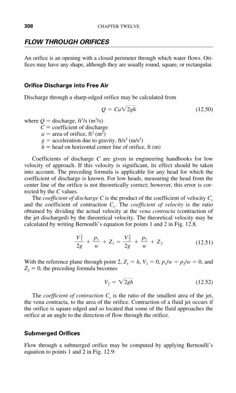
308 CHAPTER TWELVE
FLOW THROUGH ORIFICES
An orifice is an opening with a closed perimeter through which water flows. Ori-fices may have any shape, although they are usually round, square, or rectangular.
Orifice Discharge into Free Air
Discharge through a sharp-edged orifice may be calculated from
(12.50)
where Q � discharge, ft3/s (m3/s)C � coefficient of discharge a � area of orifice, ft2 (m2)g � acceleration due to gravity, ft/s2 (m/s2)h � head on horizontal center line of orifice, ft (m)
Coefficients of discharge C are given in engineering handbooks for lowvelocity of approach. If this velocity is significant, its effect should be takeninto account. The preceding formula is applicable for any head for which thecoefficient of discharge is known. For low heads, measuring the head from thecenter line of the orifice is not theoretically correct; however, this error is cor-rected by the C values.
The coefficient of discharge C is the product of the coefficient of velocity Cvand the coefficient of contraction Cc. The coefficient of velocity is the ratioobtained by dividing the actual velocity at the vena contracta (contraction ofthe jet discharged) by the theoretical velocity. The theoretical velocity may becalculated by writing Bernoulli’s equation for points 1 and 2 in Fig. 12.8.
(12.51)
With the reference plane through point 2, Z1 � h, V1 � 0, p1/w � p2/w � 0, andZ2 � 0, the preceding formula becomes
(12.52)
The coefficient of contraction Cc is the ratio of the smallest area of the jet,the vena contracta, to the area of the orifice. Contraction of a fluid jet occurs ifthe orifice is square edged and so located that some of the fluid approaches theorifice at an angle to the direction of flow through the orifice.
Submerged Orifices
Flow through a submerged orifice may be computed by applying Bernoulli’sequation to points 1 and 2 in Fig. 12.9:
V2 � �2gh
V 21
2g�
p1
w� Z1 �
V 22
2g�
p2
w� Z 2
Q � Ca�2gh

HYDRAULICS AND WATERWORKS FORMULAS 309
(12.53)
where hL � losses in head, ft (m), between 1 and 2.By assuming V1 � 0, setting h1 � h2 � �h, and using a coefficient of dis-
charge C to account for losses, the following formula is obtained:
(12.54)Q � Ca �2g �h
V2 � B2g �h1 � h2 �V 2
1
2g� hL�
1
h
Cc
2
X
Y
FIGURE 12.8 Fluid jet takes a parabolic path.
h1
2
1
h2
Δh
FIGURE 12.9 Discharge through a submerged orifice.

310 CHAPTER TWELVE
Values of C for submerged orifices do not differ greatly from those for nonsub-merged orifices.
Discharge under Falling Head
The flow from a reservoir or vessel when the inflow is less than the outflowrepresents a condition of falling head. The time required for a certain quantityof water to flow from a reservoir can be calculated by equating the volume ofwater that flows through the orifice or pipe in time dt to the volume decrease inthe reservoir. If the area of the reservoir is constant,
(12.55)
where h1 � head at the start, ft (m) h2 � head at the end, ft (m)
t � time interval for head to fall from h1 to h2, s
FLUID JETS
Where the effect of air resistance is small, a fluid discharged through an orificeinto the air follows the path of a projectile. The initial velocity of the jet is
(12.56)
where h � head on center line of orifice, ft (m); and Cv � coefficient of velocity. The direction of the initial velocity depends on the orientation of the surface
in which the orifice is located. For simplicity, the following equations weredetermined assuming the orifice is located in a vertical surface (see Fig. 12.8).The velocity of the jet in the X direction (horizontal) remains constant:
(12.57)
The velocity in the Y direction is initially zero and thereafter a function of timeand the acceleration of gravity:
(12.58)
The X coordinate at time t is
(12.59)X � Vx t � tCv �2gh
Vy � gt
Vx � V0 � Cv �2gh
V0 � Cv �2gh
t �2A
Ca �2g��h1 � �h2�
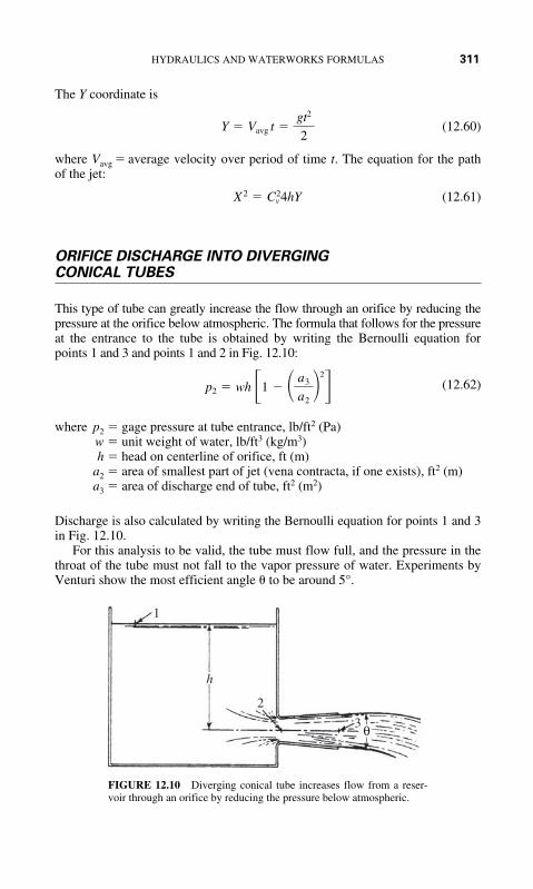
HYDRAULICS AND WATERWORKS FORMULAS 311
The Y coordinate is
(12.60)
where Vavg � average velocity over period of time t. The equation for the pathof the jet:
(12.61)
ORIFICE DISCHARGE INTO DIVERGING CONICAL TUBES
This type of tube can greatly increase the flow through an orifice by reducing thepressure at the orifice below atmospheric. The formula that follows for the pressureat the entrance to the tube is obtained by writing the Bernoulli equation forpoints 1 and 3 and points 1 and 2 in Fig. 12.10:
(12.62)
where p2 � gage pressure at tube entrance, lb/ft2 (Pa)w � unit weight of water, lb/ft3 (kg/m3)h � head on centerline of orifice, ft (m)
a2 � area of smallest part of jet (vena contracta, if one exists), ft2 (m)a3 � area of discharge end of tube, ft2 (m2)
Discharge is also calculated by writing the Bernoulli equation for points 1 and 3in Fig. 12.10.
For this analysis to be valid, the tube must flow full, and the pressure in thethroat of the tube must not fall to the vapor pressure of water. Experiments byVenturi show the most efficient angle � to be around 5°.
p2 � wh �1 � � a3
a2�
2
�
X 2 � C2v4hY
Y � Vavg t �gt2
2
1
h
2
θ3
FIGURE 12.10 Diverging conical tube increases flow from a reser-voir through an orifice by reducing the pressure below atmospheric.

312 CHAPTER TWELVE
WATER HAMMER
Water hammer is a change in pressure, either above or below the normal pres-sure, caused by a variation of the flow rate in a pipe.
The equation for the velocity of a wave in a pipe is
(12.63)
where U � velocity of pressure wave along pipe, ft/s (m/s) E � modulus of elasticity of water, 43.2 � 106 lb/ft2 (2.07 � 106 kPa)� � density of water, 1.94 lb�s/ft4 (specific weight divided by accelera-
tion due to gravity) D � diameter of pipe, ft (m) Ep � modulus of elasticity of pipe material, lb/ft2 (kg/m2)
t � thickness of pipe wall, ft (m)
PIPE STRESSES PERPENDICULAR TO THE LONGITUDINAL AXIS
The stresses acting perpendicular to the longitudinal axis of a pipe are causedby either internal or external pressures on the pipe walls.
Internal pressure creates a stress commonly called hoop tension. It may becalculated by taking a free-body diagram of a 1-in (25.4-mm)-long strip ofpipe cut by a vertical plane through the longitudinal axis (Fig. 12.11). Theforces in the vertical direction cancel out. The sum of the forces in the hori-zontal direction is
(12.64)pD � 2F
U � BE
� B1
1 � ED/Ep t
F F
D
FF
FIGURE 12.11 Internal pipe pressure produceshoop tension.

HYDRAULICS AND WATERWORKS FORMULAS 313
where p � internal pressure, lb/in2 (MPa)D � outside diameter of pipe, in (mm) F � force acting on each cut of edge of pipe, lb (N)
Hence, the stress, lb/in2 (MPa) on the pipe material is
(12.65)
where A � area of cut edge of pipe, ft2 (m2); and t � thickness of pipe wall,in (mm).
TEMPERATURE EXPANSION OF PIPE
If a pipe is subject to a wide range of temperatures, the stress, lb/in2 (MPa), dueto a temperature change is
(12.66)
where E � modulus of elasticity of pipe material, lb/in2 (MPa)�T � temperature change from installation temperature
c � coefficient of thermal expansion of pipe material
The movement that should be allowed for, if expansion joints are to be used, is
(12.67)
where �L � movement in length L of pipe, and L � length between expansionjoints.
FORCES DUE TO PIPE BENDS
It is a common practice to use thrust blocks in pipe bends to take the forces onthe pipe caused by the momentum change and the unbalanced internal pressureof the water.
The force diagram in Fig. 12.12 is a convenient method for finding the resul-tant force on a bend. The forces can be resolved into X and Y components to findthe magnitude and direction of the resultant force on the pipe. In Fig. 12.12,
V1 � velocity before change in size of pipe, ft /s (m/s)
V2 � velocity after change in size of pipe, ft /s (m/s)
p1 � pressure before bend or size change in pipe, lb/ft2 (kPa)
p2 � pressure after bend or size change in pipe, lb/ft2 (kPa)
�L � Lc �T
f � cE �T
f �F
A�
pD
2t

F2m =
Section 1
Section 2
Directionof flow
F2 = P2 A2
P1 = P1 A1
V1, P1, A1
V2, P2, A2
P2F1m
X
P1
α
α
θ
θ
F2m
Y
Y
X
R
V2Qwg Resultant
force
F1m =V1Qw
g
FIGURE 12.12 Forces produced by flow at a pipe bend and change in diameter.
314

HYDRAULICS AND WATERWORKS FORMULAS 315
A1 � area before size change in pipe, ft2 (m2)
A2 � area after size change in pipe, ft2 (m2)
F2m � force due to momentum of water in section 2 � V2Qw/g
F1m � force due to momentum of water in section 1 � V1Qw/g
P2 � pressure of water in section 2 times area of section 2 � p2A2
P1 � pressure of water in section 1 times area of section 1 � p1A1
w � unit weight of liquid, lb/ft3 (kg/m3)
Q � discharge, ft3/s (m3/s)
If the pressure loss in the bend is neglected and there is no change in magnitudeof velocity around the bend, a quick solution is
(12.68)
where R � resultant force on bend, lb (N) � � angle R makes with F1mp � pressure, lb/ft2 (kPa)w � unit weight of water, 62.4 lb/ft3 (998.4 kg/m3)V � velocity of flow, ft/s (m/s) g � acceleration due to gravity, 32.2 ft/s2 (9.81 m/s2)A � area of pipe, ft2 (m2)� � angle between pipes (0° � � � 180°)
CULVERTS
A culvert is a closed conduit for the passage of surface drainage under a high-way, a railroad, a canal, or other embankment. The slope of a culvert and itsinlet and outlet conditions are usually determined by the topography of the site.Because of the many combinations obtained by varying the entrance condi-tions, exit conditions, and slope, no single formula can be given that applies toall culvert problems.
The basic method for determining discharge through a culvert requiresapplication of the Bernoulli equation between a point just outside the entranceand a point somewhere downstream.
Entrance and Exit Submerged
When both the exit and entrance are submerged (Fig. 12.13), the culvert flows full,and the discharge is independent of the slope. This is normal pipe flow and is easilysolved by using the Manning or Darcy–Weisbach formula for friction loss.
� ��
2
R � 2A �wV2
g� p� cos
�
2

316 CHAPTER TWELVE
From the Bernoulli equation for the entrance and exit, and the Manningequation for friction loss, the following equation is obtained:
(12.69)
Solution for the velocity of flow yields
(12.70)
where H � elevation difference between headwater and tailwater, ft (m) V � velocity in culvert, ft/s (m/s) g � acceleration due to gravity, 32.2 ft/s2 (9.81 m/s2)
Ke � entrance-loss coefficient n � Manning’s roughness coefficient L � length of culvert, ft (m) R � hydraulic radius of culvert, ft (m)
The preceding equation can be solved directly because the velocity is the onlyunknown.
Culverts on Subcritical Slopes
Critical slope is the slope just sufficient to maintain flow at critical depth.When the slope is less than critical, the flow is considered subcritical.
V � BH
(1 � Ke/2g) � (n2L /2.21R4/3)
H � (1 � Ke)V 2
2g�
V 2n2L
2.21R4/3
V2
2g(1 + Ke)
Hydraulicgrade line
H
FIGURE 12.13 With entrance and exit of a culvert submerged, normal pipeflow occurs. Discharge is independent of slope. The fluid flows under pres-sure. Discharge may be determined from Bernoulli and Manning equations.

HYDRAULICS AND WATERWORKS FORMULAS 317
Entrance Submerged or Unsubmerged but Free Exit. For these conditions,depending on the head, the flow can be either pressure or open channel (Fig. 12.14).
The discharge for the open-channel condition is obtained by writing theBernoulli equation for a point just outside the entrance and a point a short dis-tance downstream from the entrance. Thus,
(12.71)
The velocity can be determined from the Manning equation:
(12.72)
By substituting this into
(12.73)
where H � head on entrance measured from bottom of culvert, ft (m) Ke � entrance-loss coefficient S � slope of energy grade line, which for culverts is assumed to equal
slope of bottom of culvert R � hydraulic radius of culvert, ft (m) dn � normal depth of flow, ft (m)
H � (1 � Ke)2.2
2gn2 SR4/3 � dn
V 2 �2.2SR4/3
n2
H � Ke
V 2
2g�
V 2
2g� dn
H
Entrance loss plus velocity head
Watersurface dc
Ddndn
S
V2
2g(1 + Ke)
FIGURE 12.14 Open-channel flow occurs in a culvert with free dischargeand normal depth dn greater than the critical depth dc when the entrance isunsubmerged or slightly submerged. Discharge depends on head H, loss atentrance, and slope of culvert.

318 CHAPTER TWELVE
To solve the preceding head equation, it is necessary to try different valuesof dn and corresponding values of R until a value is found that satisfies theequation.
OPEN-CHANNEL FLOW
Free surface flow, or open-channel flow, includes all cases of flow in which theliquid surface is open to the atmosphere. Thus, flow in a pipe is open channel ifthe pipe is only partly full.
A uniform channel is one of constant cross section. It has uniform flow if thegrade, or slope, of the water surface is the same as that of the channel. Hence,depth of flow is constant throughout. Steady flow in a channel occurs if the depthat any location remains constant with time.
The discharge Q at any section is defined as the volume of water passingthat section per unit of time. It is expressed in cubic feet per second, ft3/s (cubicmeter per second, m3/s), and is given by
(12.74)
where V � average velocity, ft/s (m/s) A � cross-sectional area of flow, ft2 (m2)
When the discharge is constant, the flow is said to be continuous and therefore
(12.75)
where the subscripts designate different channel sections. This preceding equa-tion is known as the continuity equation for continuous steady flow.
Depth of flow d is taken as the vertical distance, ft (m), from the bottom of achannel to the water surface. The wetted perimeter is the length, ft (m), of a linebounding the cross-sectional area of flow minus the free surface width. Thehydraulic radius R equals the area of flow divided by its wetted perimeter. Theaverage velocity of flow V is defined as the discharge divided by the area of flow:
(12.76)
The velocity head HV, ft (m), is generally given by
(12.77)
where V � average velocity, ft/s (m/s); and g � acceleration due to gravity, 32.2ft/s2 (9.81 m/s2).
The true velocity head may be expressed as
(12.78)HVa � �V 2
2g
HV �V 2
2g
V �Q
A
Q � V1 A1 � V2 A2 � � � �
Q � VA

HYDRAULICS AND WATERWORKS FORMULAS 319
where � is an empirical coefficient that represents the degree of turbulence.Experimental data indicate that � may vary from about 1.03 to 1.36 for pris-matic channels. It is, however, normally taken as 1.00 for practical hydraulic workand is evaluated only for precise investigations of energy loss.
The total energy per pound (kilogram) of water relative to the bottom of thechannel at a vertical section is called the specific energy head He. It is com-posed of the depth of flow at any point, plus the velocity head at the point. It isexpressed in feet (meter) as
(12.79)
A longitudinal profile of the elevation of the specific energy head is called theenergy grade line, or the total-head line (Fig. 12.15). A longitudinal profile of thewater surface is called the hydraulic grade line. The vertical distance between theseprofiles at any point equals the velocity head at that point.
Loss of head due to friction hf in channel length L equals the drop in eleva-tion of the channel �Z in the same distance.
Normal Depth of Flow
The depth of equilibrium flow that exists in the channel of Fig. 12.15 is calledthe normal depth dn. This depth is unique for specific discharge and channelconditions. It may be computed by a trial-and-error process when the channelshape, slope, roughness, and discharge are known. A form of the Manning equa-tion is suggested for this calculation:
(12.80)AR2/3 �Qn
1.486S1/2
He � d �V 2
2g
S
21
hf
SW
V2 = V1d2 = d1
S0
Hydraulic grade line
Energy grade line
Channel bottom
V1d1
Z1Z2
V22g
2g
ΔZ
Datum line
L
2 V12g
2
V12
FIGURE 12.15 Characteristics of uniform open-channel flow.

320 CHAPTER TWELVE
where A � area of flow, ft2 (m2)R � hydraulic radius, ft (m) Q � amount of flow or discharge, ft3/s (m3/s)n � Manning’s roughness coefficient S � slope of energy grade line or loss of head, ft (m), due to friction per
linear ft (m), of channel
AR2/3 is referred to as a section factor.
Critical Depth of Open-Channel Flow
For a given value of specific energy, the critical depth gives the greatest dis-charge, or conversely, for a given discharge, the specific energy is a minimumfor the critical depth.
For rectangular channels, the critical depth, dc ft (m), is given by
(12.81)
where dc � critical depth, ft (m)Q � quantity of flow or discharge, ft3/s (m3/s)b � width of channel, ft (m)
MANNING’S EQUATION FOROPEN CHANNELS
One of the more popular of the numerous equations developed for determina-tion of flow in an open channel is Manning’s variation of the Chezy formula:
(12.82)
where R � hydraulic radius, ft (m) V � mean velocity of flow, ft/s (m/s) S � slope of energy grade line or loss of head due to friction, ft/linear
ft (m/m), of channel C � Chezy roughness coefficient
Manning proposed:
(12.83)
where n is the coefficient of roughness in the Ganguillet–Kutter formula.When Manning’s C is used in the Chezy formula, the Manning equation for
flow velocity in an open channel results:
C �1.4861/6
n
V � C �RS
dc � B3 Q2
b2g

HYDRAULICS AND WATERWORKS FORMULAS 321
(12.84)
Because the discharge Q � VA, this equation may be written:
(12.85)
where A � area of flow, ft2 (m2); and Q � quantity of flow, ft3/s (m3/s).
HYDRAULIC JUMP
This is an abrupt increase in depth of rapidly flowing water (Fig. 12.16).Flow at the jump changes from a supercritical to a subcritical stage with anaccompanying loss of kinetic energy. Depth at the jump is not discontinuous.The change in depth occurs over a finite distance, known as the length ofjump. The upstream surface of the jump, known as the roller, is a turbulentmass of water.
The depth before a jump is the initial depth, and the depth after a jump isthe sequent depth. The specific energy for the sequent depth is less than that forthe initial depth because of the energy dissipation within the jump. (Initial andsequent depths should not be confused with the depths of equal energy, or alter-nate depths.)
Q �1.486
nAR2/3S1/2
V �1.486
nR2/3S1/2
Energy lossin jump ΔHe
L
DepthCritical
E.G.L. V2
V2
d2 dcd1
V1
2g
2
V12
2g
FIGURE 12.16 Hydraulic jump.

322 CHAPTER TWELVE
The pressure force F developed in hydraulic jump is
(12.86)
where d1 � depth before jump, ft (m) d2 � depth after jump, ft (m) w � unit weight of water, lb/ft3 (kg/m3)
The rate of change of momentum at the jump per foot width of channel equals
(12.87)
where M � mass of water, lb�s2/ft (kg�s2/m)V1 � velocity at depth d1, ft/s (m/s)V2 � velocity at depth d2, ft/s (m/s)q � discharge per foot width of rectangular channel, ft3/s (m3/s)t � unit of time, sg � acceleration due to gravity, 32.2 ft/s2 (9.81 kg/s2)
Then (12.88)
(12.89)
(12.90)
The head loss in a jump equals the difference in specific-energy head beforeand after the jump. This difference (Fig. 12.17) is given by
(12.91)
where He1 � specific-energy head of stream before jump, ft (m); and He2 �specific-energy head of stream after jump, ft (m).
The depths before and after a hydraulic jump may be related to the criticaldepth by
(12.92)
where q � discharge, ft3/s (m3/s) per ft (m) of channel width; and dc � criticaldepth for the channel, ft (m).
It may be seen from this equation that if d1 � dc, d2 must also equal dc.Figure 12.18 shows how the length of hydraulic jump may be computed using
the Froude number and the L /d2 ratio.
d1d2d1 � d2
2�
q2
g� d3
c
�He � He1 � He2 �(d2 � d1)3
4d1 d2
d1 ��d2
2� B
2V 22 d2
g�
d 22
4
d2 ��d1
2� B
2V 21 d1
g�
d 21
4
V 21 �
gd2
2d1 (d2 � d1)
F �MV1 � MV2
t�
qw
g (V1 � V2)
F �d2
2 w
2�
d21 w
2

HYDRAULICS AND WATERWORKS FORMULAS 323
NONUNIFORM FLOW IN OPEN CHANNELS
Symbols used in this section are V � velocity of flow in the open channel, ft/s(m/s); Dc � critical depth, ft (m); g � acceleration due to gravity, ft/s2 (m/s2);Q � flow rate, ft3/s (m3/s); q � flow rate per unit width, ft3/ft (m3/m); and Hm �minimum specific energy, ft�lb/lb (kg�m/kg). Channel dimensions are in feet ormeters and the symbols for them are given in the text and illustrations.
F1 = 1 – 1.7, Undular jump
F1 = 1.7 – 2.5, Weak jumposcillating jet
F1 = 2.5 – 4.5, Oscillating jump
F1 = 4.5 – 9.0, Steady jump
F1 = Larger than 9.0, strong jump
FIGURE 12.17 Type of hydraulic jump depends onFroude number.

7
6
5Ld2
4
3
Steady jumpUndular
jumpWeakjump
Oscillatingjump
WavySurfaceturbulence only
Bestperformance
Acceptableperformance
RollerL
d1 d2
V1
Strong jump
Expensive stilling basin andrough surface conditions
20191817161514131211109876543210
F1 = V1/√gd1
FIGURE 12.18 Length of hydraulic jump in a horizontal channel depends on sequent depth d2 and the Froude number of the approaching flow.
324

HYDRAULICS AND WATERWORKS FORMULAS 325
Nonuniform flow occurs in open channels with gradual or sudden changesin the cross-sectional area of the fluid stream. The terms gradually varied flowand rapidly varied flow are used to describe these two types of nonuniformflow. Equations are given next for flow in (1) rectangular cross-sectional chan-nels, (2) triangular channels, (3) parabolic channels, (4) trapezoidal channels,and (5) circular channels. These five types of channels cover the majority ofactual examples met in the field. Figure 12.19 shows the general energy rela-tions in open-channel flow.
Rectangular Channels
In a rectangular channel, the critical depth Dc equals the mean depth Dm; thebottom width of the channel b equals the top width T; and when the dischargeof fluid is taken as the flow per foot (meter) of width q of the channel, both band T equal unity. Then Vc, the average velocity, is
(12.93)
and (12.94)
Also, (12.95)
where g � acceleration due to gravity in USCS or SI units.
(12.96)
and (12.97)
The minimum specific energy is
(12.98)Hm � 3�2 Dc
Dc � B3 q2
g
q � �g Dc3/2
Q � �g bDc3/2
Dc �V 2
c
g
Vc � �gDc
V2
2gEnergygradient
Watersurface
Channelbottom
HeHD
ZDatum plane
FIGURE 12.19 Energy of open-channel fluid flow.

326 CHAPTER TWELVE
and the critical depth is
(12.99)
Then the discharge per foot (meter) of width is given by
(12.100)
With g � 32.16, Eq. (12.100) becomes
(12.101)
Triangular Channels
In a triangular channel (Fig. 12.20), the maximum depth Dc and the mean depthDm equal Dc. Then,
(12.102)
and (12.103)
As shown in Fig. 12.20, z is the slope of the channel sides, expressed as aratio of horizontal to vertical; for symmetrical sections, z � e/Dc. The area, a �
. Then,
(12.104)
With g � 32.16,
(12.105)
and (12.106)Dc � B5 2Q2
gz2
Q � 4.01zDc5/2
Q � Bg
2zDc
5/2
zD2c
Dc �2V 2
c
g
Vc � BgDc
2
1�2
q � 3.087H3/2m
q � �g (2�3)3/2H3/2m
Dc � 2�3 Hm
Dcz = e
Dc
Te e
FIGURE 12.20 Triangular open channel.

HYDRAULICS AND WATERWORKS FORMULAS 327
or (12.107)
With g � 32.16,
(12.108)
Parabolic Channels
These channels can be conveniently defined in terms of the top width T and thedepth Dc. Then the area a � DcT and the mean depth � Dm.
Then (Fig. 12.21),
(12.109)
and (12.110)
Further, (12.111)
With g � 32.16,
(12.112)
and (12.113)
Also, (12.114)
With g � 32.16,
(12.115)Q � 2.005TH3/2m
Q � B8g
27 � 3
4 �3/2
TH3/2m
Dc �3
2 B3 Q2
gT 2
Q � 3.087TD3/2c
Q � B8g
27TD3/2
c
Dc �3
2
V2c
g
Vc � �2�3 gDc
2�3
Q � 2.295zHm5/2
Q � Bg
2 � 4
5 �5/2
zHm5/2
T
Dc
FIGURE 12.21 Parabolic open channel.

328 CHAPTER TWELVE
Trapezoidal Channels
Figure 12.22 shows a trapezoidal channel having a depth of Dc and a bottomwidth b. The slope of the sides, horizontal divided by vertical, is z. Expressingthe mean depth Dm in terms of channel dimensions, the relations for criticaldepth Dc and average velocity Vc are
(12.116)
and (12.117)
The discharge through the channel is then
(12.118)
Then, the minimum specific energy and critical depth are
(12.119)
(12.120)
Circular Channels
Figure 12.23 shows a typical circular channel in which the area a, top width T,and depth Dc are
(12.121)a �d2
4 (�r �
1
2 sin 2�)
Dc �4zHm � 3b � 216z2H m
2 � 16zHm b � 9b2
10z
Hm �3b � 5zDc
2b � 4zDc
Dc
Q � Bg(b � zDc)3
b � 2zDc
D3/2c
Dc �V 2
c
c�
b
2z� B
V 4c
g2 �b2
4z2
Vc � Bb � zDc
b � 2zDc
gDc
d/2
θ θd/2
T Dc
FIGURE 12.23 Circular channel.
Dcz = e
Dcb
e eT
FIGURE 12.22 Trapezoidal open channel.

HYDRAULICS AND WATERWORKS FORMULAS 329
(12.122)
(12.123)
Flow quantity is then given by
(12.124)
WEIRS
A weir is a barrier in an open channel over which water flows. The edge or sur-face over which the water flows is called the crest. The overflowing sheet ofwater is the nappe.
If the nappe discharges into the air, the weir has free discharge. If the dis-charge is partly under water, the weir is submerged or drowned.
Types of Weirs
A weir with a sharp upstream corner or edge such that the water springs clear ofthe crest is a sharp-crested weir (Fig. 12.24). All other weirs are classed as weirsnot sharp crested. Sharp-crested weirs are classified according to the shape of theweir opening, such as rectangular weirs, triangular or V-notch weirs, trapezoidalweirs, and parabolic weirs. Weirs not sharp crested are classified according to theshape of their cross section, such as broad-crested weirs, triangular weirs, and (asshown in Fig. 12.25) trapezoidal weirs.
The channel leading up to a weir is the channel of approach. The meanvelocity in this channel is the velocity of approach. The depth of water produc-ing the discharge is the head.
Q �
23/2g1/2��r �1
2 sin 2��
3/2
8(sin �)1/2 (1 � cos �)5/2 D5/2c
Dc �d
2 (1 � cos �)
T � d sin �
Water surface
H
P
FIGURE 12.24 Sharp-crested weir.

330 CHAPTER TWELVE
Sharp-crested weirs are useful only as a means of measuring flowing water.In contrast, weirs not sharp crested are commonly incorporated into hydraulicstructures as control or regulation devices, with measurement of flow as theirsecondary function.
FLOW OVER WEIRS
Rectangular Weir
The Francis formula for the discharge of a sharp-crested rectangular weir hav-ing a length b greater than 3h is
(12.125)
where Q � discharge over weir, ft3/s (m3/s)b � length of weir, ft (m)h � vertical distance from level of crest of weir to water surface at point
unaffected by weir drawdown (head on weir), ft (m)n � number of end contractions (0, 1, or 2)
h0 � head of velocity of approach [equal to , where � velocity ofapproach, (ft/s) (m/s)], ft (m)
gc � 32.2 (lb mass) (ft)/(lb force) (s2)(m/s2)
If the sides of the weir are coincident with the sides of the approach channel,the weir is considered to be suppressed, and n � 0. If both sides of the weir arefar enough removed from the sides of the approach channel to permit free lat-eral approach of water, the weir is considered to be contracted, and n � 2. Ifone side is suppressed and one is contracted, n � 1.
Triangular Weir
The discharge of triangular weirs with notch angles of 30°, 60°, and 90° isgiven by the formulas in Table 12.2.
v0v02 /2gc
Q � 3.33 � b � nh
10 � [(h � h0)3/2 � h3/20 ]
Water surface
H
P
FIGURE 12.25 Weir not sharp crested.

HYDRAULICS AND WATERWORKS FORMULAS 331
Trapezoidal (Cipolletti) Weir
The Cipolletti weir, extensively used for irrigation work, is trapezoidal inshape. The sides slope outward from the crest at an inclination of 1:4 (horizontal:vertical). The discharge is
(12.126)
where b, h, and Q are as defined earlier. The advantage of this type of weir isthat no correction needs to be made for contractions.
Broad-Crested Weir
The discharge of a broad-crested weir is
(12.127)
Values of C for broad-crested weirs with rounded upstream corners generallyrange from 2.6 to 2.9. For sharp upstream corners, C generally ranges from 2.4to 2.6. Dam spillways are usually designed to fit the shape of the underside ofa stream flowing over a sharp-crested weir. The coefficient C for such a spill-way varies considerably with variation in the head, as shown in Table 12.3.
Q, b, and h are as defined for rectangular weirs.
Q � Cbh3/2
Q � 3.367bh3/2
TABLE 12.3 Variations in Head Ratio andCoefficient of Discharge for Broad-Crested Weirs
Ratio of actual head Coefficient ofto design head discharge
0.20 3.300.40 3.500.60 3.700.80 3.851.00 3.981.20 4.101.40 4.22
TABLE 12.2 Discharge of Triangular Weirs
Notch (vertex) angle Discharge formula*
90° Q � 0.685h2.45
60° Q � 1.45h2.47
30° Q � 2.49h2.48
*h is as defined above in the Francis formula.

332 CHAPTER TWELVE
PREDICTION OF SEDIMENT-DELIVERY RATE
Two methods of approach are available for predicting the rate of sediment accu-mulation in a reservoir; both involve predicting the rate of sediment delivery.
One approach depends on historical records of the silting rate for existingreservoirs and is purely empirical. The second general method of calculating thesediment-delivery rate involves determining the rate of sediment transportas a function of stream discharge and density of suspended silt.
The quantity of bed load is considered a constant function of the dischargebecause the sediment supply for the bed-load forces is always available in allbut lined channels. An accepted formula for the quantity of sediment transportedas bed load is the Schoklitsch formula:
(12.128)
where Gb � total bed load, lb/s (kg/s)Dg � effective grain diameter, in (mm)
S � slope of energy gradientQi � total instantaneous discharge, ft3/s (m3/s)b � width of river, ft (m)
qo � critical discharge, ft3/s (m3/s) per ft (m), of river width� (0.00532/S4/3)Dg
An approximate solution for bed load by the Schoklitsch formula can bemade by determining or assuming mean values of slope, discharge, and singlegrain size representative of the bed-load sediment. A mean grain size of 0.04 in(about 1 mm) in diameter is reasonable for a river with a slope of about 1.0 ft/mi(0.189 m/km).
EVAPORATION AND TRANSPIRATION
The Meyer equation, developed from Dalton’s law, is one of many evaporationformulas and is popular for making evaporation-rate calculations:
(12.129)
(12.130)
where E � evaporation rate, in 30-day monthC � empirical coefficient, equal to 15 for small, shallow pools and 11 for
large, deep reservoirsew � saturation vapor pressure, in (mm), of mercury, corresponding to
monthly mean air temperature observed at nearby stations for smallbodies of shallow water or corresponding to water temperatureinstead of air temperature for large bodies of deep water
# � 1 � 0.1w
E � C (ew � ea)#
Gb �86.7
D1/2g
S3/2 (Qi � bqo)

HYDRAULICS AND WATERWORKS FORMULAS 333
ea � actual vapor pressure, in (mm), of mercury, in air based on monthlymean air temperature and relative humidity at nearby stations forsmall bodies of shallow water or based on information obtainedabout 30 ft (9.14 m) above the water surface for large bodies of deepwater
w � monthly mean wind velocity, mi/h (km/h), at about 30 ft (9.14 m)aboveground
# � wind factor
As an example of the evaporation that may occur from a large reservoir, themean annual evaporation from Lake Mead is 6 ft (1.82 m).
METHOD FOR DETERMINING RUNOFF FOR MINORHYDRAULIC STRUCTURES
The most common means for determining runoff for minor hydraulic structuresis the rational formula:
(12.131)
where Q � peak discharge, ft3/s (m3/s)C � runoff coefficient � percentage of rain that appears as direct runoff I � rainfall intensity, in/h (mm/h)
A � drainage area, acres (m2)
COMPUTING RAINFALL INTENSITY
Chow lists 24 rainfall-intensity formulas of the form:
(12.132)
where I � rainfall intensity, in/h (mm/h)K, b, n, and n1 � coefficient, factor, and exponents, respectively, depend-
ing on conditions that affect rainfall intensityF � frequency of occurrence of rainfall, yearst � duration of storm, min
� time of concentration
Perhaps the most useful of these formulas is the Steel formula:
(12.133)I �K
t � b
I �KF n1
(t � b)n
Q � CIA

334 CHAPTER TWELVE
where K and b are dependent on the storm frequency and region of the UnitedStates (Fig. 12.26 and Table 12.4).
The Steel formula gives the average maximum precipitation rates for dura-tions up to 2 h.
GROUNDWATER
Groundwater is subsurface water in porous strata within a zone of saturation. Itsupplies about 20 percent of the United States water demand.
Aquifers are groundwater formations capable of furnishing an economicalwater supply. Those formations from which extractions cannot be made eco-nomically are called aquicludes.
75
3
26
1
3
4 4
2
FIGURE 12.26 Regions of the United States for usewith the Steel formula.
TABLE 12.4 Coefficients for Steel Formula
RegionFrequency,
years Coefficients 1 2 3 4 5 6 7
2 K 206 140 106 70 70 68 32b 30 21 17 13 16 14 11
4 K 247 190 131 97 81 75 48b 29 25 19 16 13 12 12
10 K 300 230 170 111 111 122 60b 36 29 23 16 17 23 13
25 K 327 260 230 170 130 155 67b 33 32 30 27 17 26 10

HYDRAULICS AND WATERWORKS FORMULAS 335
Permeability indicates the ease with which water moves through a soil anddetermines whether a groundwater formation is an aquifer or aquiclude.
The rate of movement of groundwater is given by Darcy’s law:
(12.134)
where Q � flow rate, gal/day (m3/day)K � hydraulic conductivity, ft/day (m/day)I � hydraulic gradient, ft/ft (m/m)
A � cross-sectional area, perpendicular to direction of flow, ft2 (m2)
WATER FLOW FOR FIREFIGHTING
The total quantity of water used for fighting fires is normally quite small, but thedemand rate is high. The fire demand as established by the American InsuranceAssociation is
(12.135)
where G � fire-demand rate, gal/min (liter/s); and P � population, thousands.
FLOW FROM WELLS
The steady flow rate Q can be found for a gravity well by using the Dupuitformula:
(12.136)
where Q � flow, gal/day (liter/day)K � hydraulic conductivity, ft/day (m/day), under 1:1 hydraulic gradientH � total depth of water from bottom of well to free-water surface before
pumping, ft (m)h � H minus drawdown, ft (m)D � diameter of circle of influence, ft (m)d � diameter of well, ft (m)
The steady flow, gal/day (liter/day), from an artesian well is given by
(12.137)
where t is the thickness of confined aquifer, ft (m).
Q �2.73Kt (H � h)
log(D/d)
Q �1.36K (H 2 � h2)
log(D/d)
G � 1020�P (1 � 0.01�P)
Q � KIA

336 CHAPTER TWELVE
ECONOMICAL SIZING OF DISTRIBUTION PIPING
An equation for the most economical pipe diameter for a distribution system forwater is
(12.138)
where D � pipe diameter, ft (m)f � Darcy–Weisbach friction factorb � value of power, $/hp per year ($/kW per year)
Qa � average discharge, ft3/s (m3/s)S � allowable unit stress in pipe, lb/in2 (MPa)a � in-place cost of pipe, $/lb ($/kg)i � yearly fixed charges for pipeline (expressed as a fraction of total
capital cost)Ha � average head on pipe, ft (m)
VENTURI METER FLOW COMPUTATION
Flow through a venturi meter (Fig. 12.27) is given by
(12.139)
(12.140)K �4
B2g
1 � (d2�d1)2
Q � cKd 22 2h1 � h2
D � 0.215 � fbQ3a S
aiHa�
1/7
Throat
Throat connection
Flow-rate scaleMain connection
Main section
21°
5
5°–7°
4321
h1 – h2
FIGURE 12.27 Standard venturi meter.

HYDRAULICS AND WATERWORKS FORMULAS 337
where Q � flow rate, ft3/s (m3/s)c � empirical discharge coefficient dependent on throat velocity and
diameterd1 � diameter of main section, ft (m)d2 � diameter of throat, ft (m)h1 � pressure in main section, ft (m) of waterh2 � pressure in throat section, ft (m) of water
HYDROELECTRIC POWER GENERATION
Hydroelectric power is electrical power obtained from conversion of potentialand kinetic energy of water. The potential energy of a volume of water is theproduct of its weight and the vertical distance it can fall:
(12.141)
where PE � potential energyW � total weight of the waterZ � vertical distance water can fall
Power is the rate at which energy is produced or utilized:
1 horsepower (hp) � 550 ft�lb/s
1 kilowatt (kW) � 738 ft�lb/s
1 hp � 0.746 kW
1 kW � 1.341 hp
Power obtained from water flow may be computed from
(12.142)
(12.143)
where kW � kilowatthp � horsepowerQ � flow rate, ft3/s (m3/s)w �unit weight of water � 62.4 lb/ft3 (998.4 kg/m3)h � effective head � total elevation difference minus line losses due to
friction and turbulence, ft (m)% � efficiency of turbine and generator
kW �%Qwh
738�
%Qh
11.8
hp �%Qwh
550�
%Qh
8.8
PE � WZ

338 CHAPTER TWELVE
PUMPS AND PUMPING SYSTEMS
Civil engineers use centrifugal and other rotating pumps for a variety oftasks—water supply, irrigation, sewage treatment, fire-fighting systems, shipcanals—and numerous other functions. This section of Chap. 12 presents per-tinent formulas for applying rotating pumps for these, and other tasks.Reciprocating-pump formulas are excluded because such pumps do not findmajor usage in large civil-engineering projects. Their prime usage is as meter-ing and control dispensers in sewage treatment. The formulas given in thissection are the work of Metcalf & Eddy, Inc., written and edited by GeorgeTchobanoglous, Professor of Civil Engineering, University of California,Davis, at the time of their preparation.
Capacity
The capacity (flowrate) of a pump is the volume of liquid pumped per unit oftime, which usually is measured in liters per second or cubic meters per second(gallons per minute or million gallons per day).
Head
The term head is the elevation of a free surface of water above or below a ref-erence datum.
In pump systems, the head refers to both pumps and pump systems havingone or more pumps and the corresponding piping system. The height to whicha pump can raise a liquid is the pump head and is measured in meters (feet) ofthe flowing liquid. The head required to overcome the losses in a pipe systemat a given flowrate is the system head.
Terms applied specifically to the analysis of pumps and pump systemsinclude (1) static suction head, (2) static discharge head, (3) static head, (4)friction head, (5) velocity head, (6) minor head loss, and (7) total dynamichead, which is defined in terms of the other head terms. Each of these terms isdescribed in the following and is illustrated graphically in Fig. 12.28. All theterms are expressed in meters (feet) of water.
Static Suction Head. The static suction head hs is the difference in elevationbetween the suction liquid level and the centerline of the pump impeller. If thesuction liquid level is below the centerline of the pump impeller, it is a staticsuction lift.
Static Discharge Head. The static discharge head hd is the difference inelevation between in discharge liquid level and the centerline of the pumpimpeller.
Static Head. Static Hstat is the difference in elevation between the staticdischarge and static suction liquid levels (hd – hs).

FIGURE 12.28 Definition sketch for the head on a pump. (Metcalf & Eddy—Wastewater Engineering: Collection and Pumping ofWastewater, McGraw-Hill.)
hd
hs
Ho
hfd + Σhmd
hfs + Σhms Ht
Hs
Vs2
Motor
Ent
ranc
e lo
ss
Suction intake
Energy grade line
Datum
Pumpdischarge
Pump
Hydraulic grade line
Hstat
2g
Vd2
2g
Vd2
2g
339

340 CHAPTER TWELVE
Friction Head. The head of water that must be supplied to overcome thefrictional loss caused by the flow of fluid through the piping system is the frictionhead. The frictional head loss in the suction (hfs) and discharge (hfd) pipingsystem may be computed with the Darcy-Weisbach or Hazen-Williamsequations, discussed earlier in this chapter.
Velocity Head. The velocity head is the kinetic energy contained in the liquidbeing pumped at any point in the system and is given by
(12.144)
where V � velocity of fluid, m(ft)g � acceleration due to gravity 9.81 m/s2 (32.2 ft/s2)
In determining the head at any point in a piping system, the velocity head mustbe added to the gage reading.
Minor Head Loss. The head of water that must be supplied to overcome theloss of head through fittings and valves is the minor head loss. Minor losses inthe suction (hms) and discharge (hmd) piping system are usually estimated asfractions of the velocity head by using the following expression:
(12.145)
where hm � minor head loss, m (ft)K � head loss coefficient
Typical values of K for various pipeline fittings and appurtenances are pre-sented in standard textbooks and reference works on hydraulics.
Total Dynamic Head. The total dynamic head Ht is the head against which thepump must work when water or wastewater is being pumped. The total dynamichead on a pump, commonly abbreviated TDH, can be determined by consideringthe static suction and discharge heads, the frictional head losses, the velocityheads, and the minor head losses. The expression for determining the totaldynamic head on a pump is given in Eq. (12.146):
(12.146)
(12.147)
(12.148)HS � hs � hfs � hms �V2
s
2g
HD � hd � hfd � hmd
Ht � HD � HS �V2
d
2g�
V2s
2g
hm � KV2
2g
Velocity head �V2
2g

HYDRAULICS AND WATERWORKS FORMULAS 341
where Ht � total dynamic head, m (ft)Hd (HS) � discharge (suction) head measured at discharge (suction) nozzle
of pump referenced to the centerline of the pump impeller, m (ft)Vd (Vs) � velocity in discharge (suction) nozzle, m/s (ft/s)
g � acceleration due to gravity, 9.81 m/s2 (32.2 ft/s2)hd (hs) � static discharge (suction) head, m (ft)
hfd (hfg) � frictional head loss in discharge (suction) piping, m (ft)hmd (hms) � minor fitting and valve losses in discharge (suction) piping
system, m (ft). Entrance loss is included in computing theminor losses in the suction piping.
The reference datum for writing Eq. (12.146) is taken as the elevation of thecenterline of the pump impeller. In accordance with the standards of theHydraulic Institute, distances (heads) above datum are considered positive; dis-tances below datum are considered negative.
In terms of the static head, Eq. (12.146) can be written as
(12.149)
where Ht � total dynamic head, m (ft)Hstat � total static head, m (ft)
� hd – hs
In Eq. (12.149), the energy in the velocity head is usually considered tobe lost at the outlet of the piping system. In practice, this loss of energy is takenas being equivalent to the exit loss and is included as a minor loss.
The energy (Bernoulli’s) equation can also be applied to determine the totaldynamic head on the pump. The energy equation written between the suctionand discharge nozzle of the pump is
(12.150)
where Ht � total dynamic head, m (ft)Pd (Ps) � discharge (suction) gage pressure, kN/m2 (lbf /ft
2)� � specific weight of water, N/m3 (lbf /ft
3)Vd (Vs) � velocity in discharge (suction) nozzle, m/s (ft/s)
g � acceleration due to gravity, 9.81 m/s2 (32.2 ft/s2)zd (zs) � elevation of zero of discharge (suction) gage above datum, m (ft)
Head losses within the pump are incorporated in the total dynamic head term inEq. (12.150).
Pump Efficiency and Power Input
Pump performance is measured in terms of the capacity that a pump can dis-charge against a given head and at a given efficiency. The pump capacity is a
Ht �Pd
��
V2d
2g� zd �
Ps
��
V2s
2g� zs
V 2d�2g
Ht � Hstat � hfs � hms � hfd � hmd �V2
d
2g

342 CHAPTER TWELVE
function of the design. Information on the design is furnished by the pump manu-facturer in a series of curves for a given pump. Pump efficiency Ep—the ratio ofthe useful output power of the pump to the input power to the pump—is given by
(SI units) (12.151)
(U.S. customary units) (12.152)
where Ep � pump efficiency, dimensionlessPi � power input, kW, kN�m/s� � specific weight of water, kN/m3 (lb/ft3)Q � capacity, m3/s (ft3/s)Ht � total dynamic head, m (ft)
bhp � brake horsepower550 � conversion factor for horsepower to ft�lbf /s
Pump efficiencies usually range from 60 to 85 percent.
Characteristic Relationships for Centrifugal Pumps
The relationships described in the following are used to predict the perfor-mance of centrifugal pumps at rotational speeds other than those for whichpump characteristic curves (pump curves) were developed.
Flow, Head, and Power Coefficients. In centrifugal pumps, similar flowpatterns occur in a series of geometrically similar pumps. By applying theprinciples of dimensional analysis and the procedure proposed by Buckingham,the following three independent dimensionless groups can be derived to describethe operation of rotodynamic machines including centrifugal pumps:
(12.153)
(12.154)
(12.155)
where CQ � flow coefficientQ � capacityN � speed, rev/minD � impeller diameter
CH � head coefficientH � head
CP � power coefficientP � power input
CP �P
N3D5
CH �H
N2D2
CQ �Q
ND3
Ep �pump output
bhp�
�QHt
bhp � 550
Ep �pump output
Pi
��QHt
Pi
HYDRAULICS AND WATERWORKS FORMULAS 343
The operating points at which similar flow patterns occur are called corre-sponding points; the Eqs. (12.153) to (12.155) apply only to correspondingpoints. However, every point on a pump head-capacity curve corresponds to apoint on the head-capacity curve of a geometrically similar pump operating atthe same speed or a different speed.
Affinity Laws. For the same pump operating at a different speed, the diameterdoes not change and the following relationships can be derived from Eqs. (12.153)through (12.155):
(12.156)
(12.157)
(12.158)
These relationships, collectively known as the affinity laws, are used todetermine the effect of changes in speed on the capacity, head, and power of apump.
Specific Speed. For a geometrically similar series of pumps operating undersimilar conditions, the specific speed is
(12.159)
where Ns � specific speedN � speed, rev/minQ � capacity, m3/s (gal/min)H � head, m (ft)
To obtain the specific speed based on U.S. customary units of head andcapacity, multiply the specific speed based on metric units of head and capacityby 52.
For any pump operating at any given speed, Q and H are taken at the pointof maximum efficiency. When using Eq. (12.159) for pumps having double-suction impellers, one-half of the discharge is used, unless otherwise noted. Formultistage pumps, the head is the head per stage.
Cavitation
When determining if cavitation will be a problem, two different net positivesuction heads (NPSH or hsv) are used. The NPSH available (NPSHA) is theNPSH available in the system at the eye of the impeller. The NPSH required(NPSHR) is the NPSH required at the pump to prevent cavitation in the pump.The NPSHA is the total absolute suction head, as given by Eq. (12.149) above
Ns �C1�2
Q
C1�2H
�(Q�ND3)1�2
(H�N2D2)3�4 �NQ1�2
H3�4
P1
P2�
N31
N32
H1
H2�
N21
N22
Q1
Q2�
N1
N2

344 CHAPTER TWELVE
the vapor pressure of the water, expressed in meters (feet). Cavitation occurswhen the NPSHA is less than the NPSHR. The NPSHA is found by adding theterm to the right-hand side of Eq. (12.148) or to the energy(Bernoulli’s) equation applied to the suction side of the pump. Thus,
(12.160)
(12.161)
where NPSHA � available net positive suction head, m (ft)Patm � atmospheric pressure, N/m2 (lbf /ft
2)Pvapor � absolute vapor pressure of water, N/m2 (lbf /ft
2)� � specific weight of water, N/m3 (lbf /ft
2)
In the computation of NPSHA, including the velocity head, at the suctionnozzle is somewhat illogical because it is not a pressure available to preventvaporization of the liquid. However, in practice this term cancels out because itis also included in the NPSH required by the pump.
HYDRAULIC TURBINES*
Generation of electricity by hydraulic turbines is gaining popularity because ofthe emphasis on global warming and “clean” power. Hydro power is consideredas one of the cleanest, nonpolluting sources of electricity available today,alongside wind turbines and solar panels. Using the nomenclature below:
D � diameter of runner, in (mm)
d � jet diameter of impulse turbine, in (mm)
e � overall efficiency of turbine
eh � hydraulic efficiency (including draft tube)
em � mechanical efficiency
g � acceleration of gravity
H � net effective head, ft (m)
h � head change due to load change, ft (m)
n � rpm
n1 � rpm at 1 ft head
ns � specific speed
P � horsepower (kW)
P1 � horsepower at 1 ft head � P�H3/2
� n�P�H5/4 � n1�P1
� n��H
� eh � em
V 23 �2g
NPSHA �Ps
��
V2s
2g� zs �
Patm
��
Pvapor
�
NPSHA � hs � hfs � hms �V2
3
2g�
Patm
��
Pvapor
�
Patm�� � Pvapor��
*Marks, Mechanical Engineer’s Handbook, McGraw–Hill.

HYDRAULICS AND WATERWORKS FORMULAS 345
Q � discharge, cfs (cu m/s)
Q1 � discharge at 1 ft head cfs (cu m/s)
t � thickness, in, or time, sec
u � circumferential velocity of a point on runner, fps (m/s)
V � absolute velocity of water, fps (m/s)
Vu � tangential component of absolute velocity � V cos �
Vr � component of V in radial plane
v � velocity of water relative to runner, fps (m/s)
w � weight of water per cu ft (cu m)
The theoretical horsepower PT of a hydraulic turbine can be expressed as
(12.162)
The actual horsepower of a hydraulic turbine is the theoretical horsepowermultiplied by the turbine efficiency e,
(12.163)
(12.164)
(12.165)
(12.166)
(12.167)
(12.168)
The laws of proportionality for homologous turbines are:
For constant For constant For variablerunner diam head diam and head
P & H3/2 P & D2 P & D2H3/2
n & H1/2 n & 1/D n & H1/2DQ & H1/2 Q & D2 Q & D2H1/2
Selecting the Turbine Rotative Speed
The speed should be as high as practicable as higher the speed the lessexpensive will be the turbine and generator and the more efficient will be thegenerator.
e � over-all efficiency of turbine � eh � em
ns � specific speed � n�P�H5/4 � n1�P1
n1 � rpm at 1 ft head � n��H
Q1 � discharge at 1 ft head � Q��H, cfs
P1 � horsepower at 1 ft head � P�H3/2
P � ePT � eHQ�8.82
PT � HQw�550 � HQ�8.82
� Q��H,

346 CHAPTER TWELVE
A convenient way of determining the highest practicable speed is by therelation of the specific speed to the head. For Francis turbines this is
USCS (12.169)
SI
For propeller-type turbines, USCS (12.170)
SI
Affinity Laws. The relationships between head, discharge, speed, horsepower,and diameter are shown in the following equations, where Q � rate of discharge,H � head, N � speed, hp � horsepower, D � diameter, and subscripts denotetwo geometrically similar units with the same specific speed:*
(12.171)
(12.172)
(12.173)
(12.174)
Most designs used are tested as exact homologous models, and performance isstepped up from the model by the normal affinity laws given above.
Water Hammer in Penstocks.† If a gate movement is considered as a seriesof instantaneous movements with a very small interval between eachmovement, the pressure variation in the penstock following the gatemovement will be the effect of a series of pressure waves, each caused by oneof the instantaneous small gate movements. For a steel penstock, the velocityof the pressure wave (USCS) (SI), where d is the penstock diameter, in (m); and t is the penstock wallthickness, in (m). The pressure change at any point along the penstock at anytime after the start of the gate movement may be calculated by summing upthe effect of the individual pressure waves.
Approximate formulas (De Sparre) for the increase in pressure h, ft (m), fol-lowing gate closure, are Eqs. (12.175) through (12.177). They are quite accu-rate for pressure rises not exceeding 50 percent of the initial pressure, whichincludes most practical cases.
for (12.175)K � 1, N � 1h � aV�g
(1,420��1 � d�100t)a � 4,660�21 � d�100t
hp1
N13D1
5 �hp2
N23D2
5
N12D1
2
H1�
N22D2
2
H2
Q12
H1D14 �
Q22
H2D24
Q1
N1D31
�Q2
N2D32
� 2,100�2H
ns � 1,000�2H
� 1,900�2H
ns � 900�2H
*Karrasik—Pump Handbook, McGraw–Hill.†Marks, Mechanical Engineer’s Handbook, McGraw–Hill.

HYDRAULICS AND WATERWORKS FORMULAS 347
for (12.176)
for (12.177)
where V and H are the penstock velocity, ft/s (m/s);and head, ft (m), prior to closure; L is the penstock length, ft (m); and T is thetime of gate closure. For full load rejection, T may be taken as 85 percent of thetotal gate traversing time to allow for nonuniform gate motion.
For pressure drop following a complete gate opening, the following formula(S. Logan Kerr) may be used with T not less than 2L/a:
ft (m) (12.178)
Speed Rise Following Load Reduction.* For sudden load reductions in theelectrical system that a hydraulic turbine serves, the approximate speed rise is
(USCS) (12.179)
(SI)
where nt is the speed, rpm, at the end of time Tt; n is the speed, rpm, before theload decrease; Tt is the time interval, seconds, for the governor to adjust the flowto the new load; Pt is the reduction in load, hp (kW); h is the head rise caused bythe retardation of the flow, ft (m); H is the net effective head before the loadchange, ft (m); WR2 is the product of the revolving parts weight, lb, and thesquare of their radius of gyration, ft; and GD2 is the product of the revolvingparts weight, kg, and the square of their diameter of gyration, m.
Speed Drop Following Load Increase. For sudden load increases in theelectrical system that a hydraulic turbine serves, the approximate speed drop is
(USCS) (12.180)
(SI)
where Pt is the actual load increase and h is the head drop caused by theincrease of the flow. If the speed drop is to be determined for a given increasein gate opening, the governor time Tt for making this increase and the normalchange in load for the change in gate opening, under constant head H, can beused in the following formula:
(USCS) (12.181)
(SI)
The actual change in load, however, will be Pt (1 � h�H)3�2.
� [1 � 365,000TtPt (1 � h�H)3�2�GD2n2]1�2
nt �n � [1 � 1,620,000TtPt (1 � h�H)3�2�WR2n2]1�2
� [1 � 365,000TtPt�GD2n2 (1 � h�H)3�2]1�2
nt�n � [1 � 1,620,000TtPt�WR2n2 (1 � h�H)3�2]1�2
� [1 � 365,000TtPt (1 � h�H)3�2�GD2n2]1�2
nt�n � [1 � 1,620,000TtPt (1 � h�H)3�2�WR2n2]1�2
h �aV
g � �K � �K2 � N2
N2 � � pressure drop,
K � aV�(2gH); N � aT�(2L).
K 1, N 1h � aV�[g(2N � K)]
K � 1, N 1h � aV�{g[N � K(N � 1)]}
*Marks—Mechanical Engineer’s Handbook, McGraw-Hill.

348 CHAPTER TWELVE
DAMS
A structure that bars or detains the flow of water in an open channel or water-course. Dams are constructed for several principal purposes. Diversion damsdivert water from a stream; navigation dams raise the level of a stream toincrease the depth for navigation purposes; power dams raise the level of astream to create or concentrate hydrostatic head for power purposes; and stor-age dams store water for municipal and industrial use, irrigation, food control,river regulation, recreation, or power production. A dam serving two or morepurposes is called a multiple-purpose dam. Dams are commonly classified bythe material from which they are constructed, such as masonry, concrete, earth,rock, timber, and steel.*
Gravity Dams†
Any dam that does not depend on arch action to resist the forces imposed onit might be termed a gravity dam. The term, however, is customarilyrestricted to solid masonry or concrete dams of roughly triangular sectionwhich are straight or only slightly curved in plan. Dams of this type dependfor their stability almost entirely upon their own weight and, in spite of theirimpressive bulk, have a small factor of safety. This fact must be kept con-stantly in mind at all stages in the design and construction of a gravity dam,(Fig. 12.29).
Water Pressure. The unit pressure of water increases in proportion to itsdepth. The horizontal force due to water pressure can thus be represented by atriangular load whose resultant is at two-thirds of the distance from the watersurface to the base of the section under consideration. The formula for this waterpressure, Fig. 12.29, is:
(12.182)
where H � total height of dam from base to crest, ft (m)h � height of section considered to water surface, depth of water, ft (m)b � base or thickness of dam from the face to the back measured
horizontally, ft (m)e � eccentricity, distance from point of application of resultant to
center of base, ft (m)y1 � distance from center of base to downstream face, ft (m)y2 � distance from center of base to upstream face, ft (m)w � density of water, 62.5 lb/cu ft (kg/cu m)R � resultant, foundation reaction, or equilibrant, lb (N)F � total force, see Fig. 12.29 for subscripts, lb (N)
F2 � 1/2 wh2
*Encyclopedia of Science and Technology, McGraw-Hill.†Davis—Handbook of Applied Hydraulics, McGraw–Hill.

HYDRAULICS AND WATERWORKS FORMULAS 349
U � total uplift forceH � algebraic summation of all active horizontal forcesV � algebraic summation of all active vertical forcesM � algebraic summation of all moments�z� vertical normal stress
�1 � first principal stress�2 � second principal stress!zy � horizontal and vertical shearing stress
� � angle made by downstream face with vertical� � angle made by upstream face with verticala � ratio of acceleration due to earthquake forces to the acceleration of
gravityf � sliding factor
f � � coefficient of maximum static friction between two surfacesq � unit shear resistance of foundation materialQ � shear-friction factor of safety
F8
F3
F5
H
F6
F4
F1 F6
F8
F2
F7
Max water surface
Tailwater surface
RU
FIGURE 12.29 External forces acting on gravity dam. (Davis—Handbook of HydraulicsMcGraw-Hill.)

350 CHAPTER TWELVE
The resistance of a gravity dam to sliding is primarily dependent upon thedevelopment of sufficient shearing strength. The factor of safety due to com-bined shearing and sliding resistance may be expressed by the formula.
(12.183)
In practice, this resistance is attained in part by stepping the foundation andby measures taken to ensure bond between concrete and rock and successivepours of concrete.
Structural Analysis. In final designs for high gravity dams, considerationshould be given to combined beam and cantilever action, the effect of rockmovements and the effects of twist and beam action along sloping abutments inaddition to the conventional stability and stress analyses.
Ordinarily the following steps will suffice:
1. Compute the righting and overturning moments on selected horizontal planes,taking into consideration all of the forces which may act on the section.
2. Compute the vertical normal stresses �x on each selected plane of analysis bythe formulas
�x max (at downstream face) (12.184)
�x min (at upstream face) (12.185)
Vertical normal stresses may be assumed to have straight-line variationbetween the toe and the heel. Usually these stresses are computed on theassumption that no uplift pressure is acting on the base.
3. Compute the principal and shearing stresses at the downstream face. The firstprincipal stress in which � � the angle between the down-stream face and the vertical. The horizontal shearing stress at the toe is
4. Estimate the probable distribution of uplift pressure on the foundation, anddetermine its effects upon the stability of the section.
5. Considering the effects of uplift on the sliding factor, compute the shear-friction factor of safety and the factor of safety against overturning.
Arch Dam
An arch dam is a curved dam that carries a major part of its water load horizon-tally to the abutments by arch action, the part so carried being primarily depen-dent on the amount of curvature. Massive masonry dams, slightly curved, are
!x � �xtan� .
�1 � �x�cos2�
�V
144b �1 �6e
b �
�V
144b �1 �6e
b �
Q �[(V � U) � f �] � (b � q)
H

HYDRAULICS AND WATERWORKS FORMULAS 351
usually considered as gravity dams, although some parts of the loads may becarried by arch action. Many early arch dams were built of rubble, ashlar, orcyclopean masonry. However, practically all arch dams constructed duringrecent years have been built of concrete. Arch principles have been used indams since about 2000 B.C.
Full Load on Arches. Formulas for analyzing circular arches of constantthickness, under uniform radial loads, have been developed by various engineers.The studies made by William Cain were especially noteworthy. Slightlymodified forms of Cain’s equations for thrust and moment at the crown andabutment sections, due to uniform water loads, are as follows:
Thrust at crown, (12.186)
Moment at crown, (12.187)
Thrust at abutments, (12.188)
Moment at abutments, (12.189)
In these formulas, r is the radius to the center line of the arch, p the normalradial pressure at the center line, t the horizontal arch thickness, and ' the anglebetween the crown and abutment radii. The center-line pressure p is the extra-dos pressure times the ratio of the upstream radius to the center-line radius (seeFig. 12.30).
If shear is neglected, values of D are given by the equation
(12.190)
In order to simplify the formulas for crown thrust, D has been used in lieu of thelengthy right-hand part of Eq. 12.190, which appears in the original formulas.
When shear is included, D is replaced by Ds, the value of which is given by
(12.191)
Thrusts and moments having been calculated, intrados and extrados stressesmay be found by the usual formula
(12.192)S �H
t�
6M
t2
Ds � �1 �t2
12r2 � w �w �sin 2w
2 � � 2 sin2w � 3.00t2
12r2w�w �
sin 2w
2 �
D � �1 �t2
12r2 � w �w �sin 2w
2 � � 2 sin2w
Mα � r(pr � H0)� sin w
w� cos w�
Hα � pr � (pr � H0) cos w
M0 � � (pr � H0)r�1 �sin w
w �
H0 � pr �pr
D2w sin w
t2
12r2

352 CHAPTER TWELVE
Rock Movements. Considerations of rock movements and their effects on thesection of arch dams may be based on approximate formulas.* If the ends of thearch elements are vertical, and the bases of the cantilever elements, horizontal,rock rotations and deflections of elements with parallel sides 1 ft apart may becalculated by the following equations:
Rotation due to moment, (12.193)
Deflection due to thrust, (12.194)
Deflection due to shear, (12.195)
Rotation due to twist, (12.196)
Rotation due to shear (12.197)
Deflection due to moment, (12.198)�� �MK5
Ert
α� �VK5
Ert
�� �MtK4
Ert2
�� �VK3
Er
β� �HK2
Er
α� �MK1
Ert2
FIGURE 12.30 Constant-thickness circular arch, fixed at abutments. (Davis—Handbook of Hydraulics, McGraw-Hill.)
pP Extrados
Center line
Intrados
Mo
Hot
Cro
wn
Center ofcurvature
Abutment
Ha R a
R d
r
Maφ
*Vogt, Fredrik—Ueber dis Berehnung der Fundamentdeformation, Det Norske Videnskapa-akademi.

HYDRAULICS AND WATERWORKS FORMULAS 353
In the preceding equations, M and V are the arch and cantilever momentsand shears, H the arch thrust, Mt the cantilever twisting moment, Er the elasticmodulus of the rock, t the radial thickness of the element, and K1, K2, K3, K4,and K5 constants depending on Poisson’s ratio and the ratio of the averagelength of the dam b to the average width a. Table 12.5 gives values of K con-stants for a Poisson’s ratio of 0.20 and different values of b/a.
Formulas given in Eqs. (12.193) to (12.198) give movements at the ends ofthe arch and cantilever elements. Equation (12.194) gives horizontal movementscaused by arch thrusts. Vertical movements at cantilever bases and twist move-ments at arch abutments are not needed. Equation (12.196) gives twist move-ments at cantilever bases. Rotations and deflections given by Eqs. (12.197) and(12.198) are of a secondary nature and relatively unimportant.
Buttress Dams
The principal structural elements of a buttress dam are the water-supportingupstream face, or deck, and the buttresses. These water-bearing upstream mem-bers are supported on the buttresses and span between them; the buttresses areequally spaced triangular walls proportioned to transmit to the foundation thewater load and the weight of the structure, Fig. 12.31.
For a buttress dam, the normal foundation pressure on the horizontal planeis obtained from the well-known law of the trapezoid:
(12.199)�x �maxmin � �
N
A�
MY
I
TABLE 12.5 Values of K Constants in Eqs. (12.193) to (12.198) for Poisson’s Ratio � 0.20
Values of K
Values of b/a K1 K2 K3 K4 K5
1.0 4.32 0.62 1.02 4.65 0.3451.5 4.65 0.78 1.23 4.80 0.4132.0 4.84 0.91 1.39 5.18 0.4583.0 5.04 1.10 1.60 5.64 0.5154.0 5.15 1.25 1.77 5.90 0.550
5.0 5.22 1.36 1.89 6.08 0.5746.0 5.27 1.47 2.00 6.20 0.5928.0 5.32 1.63 2.17 6.37 0.614
10.0 5.36 1.75 2.31 6.46 0.63015.0 5.41 1.98 2.55 6.59 0.653
20.0 5.43 2.16 2.72 6.66 0.668
Vogt, Fredrik—Ueber dis Berehnung der Fundamentdeformation, Det Norske Videnskapa-akademi.

354 CHAPTER TWELVE
where �x � intensity of normal stress on horizontal planeN � total vertical load on section (masonry � water)A � sectional area of baseM � moment � Nee � eccentricity (distance from point of application to center of gravity
of section)Y � distance from center of gravity to most remote fiberI � moment of inertia of horizontal section
Either USCS or SI units can be used in this formula.
Dams on Soft or Porous Foundations. The foundation material beneath thedam may be viewed as a conduit (often called a pipe) connecting the reservoirupstream with the tailwater downstream. The objective of the designer is to makethis conduit long enough and to create within it enough friction to reduce watervelocities below values capable of moving foundation material.
An the length of water travel beneath the dam is decreased, both the velocityand head of the water increase until ultimately a channel or pipe is formedbeneath the dam. Complete failure may follow such a break.
Darcy’s law furnishes a theoretical basis for providing adequate length ofwater travel beneath a dam. This relation may be expressed as
(12.200)Q � C1HA
L
H
D
a
1110
Flow lines
Equipotentiallines
Buttresses@15'–0"c.c.
Axi
s of
dam
93765
5
4
4
3
2
2
1
1
12 13 14 1516
1718
FIGURE 12.31 Buttress dam flow net diagram. (Davis—Handbook of Hydraulic,McGraw-Hill.)

HYDRAULICS AND WATERWORKS FORMULAS 355
where Q � discharge, cfsH � head, ftL � length, ft
C1 � a coefficient that depends on the character of the materialSubstituting for Q, the value Av [Eq. 12.200] becomes
(12.201)
For each class of foundation material, homogeneity being assumed, there is adefinite maximum velocity Vn, at which the water can emerge below the damwithout carrying away foundation material and causing the failure of the structure.This value of Vn may be combined with C1 to form a new coefficient
Substituting C2 in Eq. (12.201) for C1/V, there results
(12.202)
where Ln � minimum safe length of travel pathC2 � a coefficient depending upon the foundation material
One way to avoid the possibility of a dam being carried away by the flow ofwater under it is shown in Fig. 12.31. From the flow net diagram and Darcy’slaw of flow through soils, the approximate uplift pressures and percolationvelocities can be computed.
If the number of equipotential divisions N1 in Fig.12.31 is 18, and the num-ber of flow channels N2 bounded by flow lines is 5, then
Hydraulic gradient per unit head (12.203)
For a soil of permeability k, void ratio e, and specific gravity s, the flowunder a head H is
(12.204)
At a point a (Fig.12.31) at a depth D, below the surface, a saturated founda-tion and flow path L being assumed, the total pressure is calculated as follows:
Let P � total stress per unit area
Pe � effective stress per unit area
Pn � neutral stress per unit area
� specific gravity of water
Then (12.205)
(12.206)pn � D�w �D
LH�w
p � D� s � e
1 � e ��w
�w
Q � kHN1
N2
i �N1
N2
Ln � C2H
C2 � C1�Vn.
L � C1H
V

356 CHAPTER TWELVE
and the effective stress in the soil
(12.207)
but 1/L i and i � N1/N2, therefore
(12.208)
Were the soil structure of such a nature and the reservoir head H greatenough to create a large amount of percolation or high seepage pressure, theflow Q would exceed the limits for a safe foundation and the effective pressurePe would be reduced enough to permit soil distortion and sliding of the founda-tion material upon itself.
To reduce under-dam seepage a cutoff wall, Fig. 12.31, can be used. Then,Darcy’s law, as modified to include the Schliter formula, gives the followingformula for the depth of the cutoff wall:
(12.209)
in which d � depth of cutoff, ft (m)K � a transmission constantH � head, ft (m)P � porosity of the material expressed as a decimalV � permissible velocity, fpm (m/s)b � effective base width of the dam, ft (m)
Earth Dams
Earth dams, dikes, and levees are the commonest structures used to impoundwater, and innumerable instances of their use exist in all parts of the world. Theentire range in soils, from clays to boulders or quarried stone, has been used intheir construction.
Seepage in earth dams through the dam itself and the foundation, should bekept within the limits prescribed by use of the reservoir, and by economic con-siderations. The flow of water through all soils except the coarser ones is of thelaminar type and is in accordance with Darcy’s law:
(12.210)
where Q � quantity of flow in time, tk � coefficient of permeabilityi � hydraulic gradient expressed as head lost per unit length of flow path
A � superficial area of flow (total cross-sectional area of flow, notmerely cross-sectional area of soil pores)
Q � kiAt
d �KH
2PV�
b2PV
2KH
pe � D�w� s � 1
1 � e�
N1
N2H�
(
pe � p � pn � D� s � e
1 � e ��w � D�w � DH
L�w

HYDRAULICS AND WATERWORKS FORMULAS 357
The coefficient of permeability may be determined in the laboratory by testson distributed or remolded samples of the soil.
Quantity of Seepage. The quantity of seepage can be computed directlyfrom a flow net. Or, in certain instances, from charts or equations without theconstruction of a flow net. The formula for computing the quantity of seepagefrom a flow net is
(12.211)
where Q � quantity of seepage in length of dam under considerationk � effective coefficient of permeability which is nf � number of flow channels of netnd � number of equipotential drops of netht � head difference between headwater and tail waterL � length of dam to which the flow net applies
The ratio nf / nd is termed the shape factor of the flow net.Approximate solutions for the quantity of seepage underneath an impervi-
ous embankment founded on a pervious foundation have been developed byTerzaghi. The definitions of terms for the equations are as given above or asdefined in Fig. 12.32:
Case I. When I > 2U,
(12.212)Q � � hk
0.88 �I
U
L�
�kmaxkmin
Q � knf
nd
htL
Pervious
Line of seepage
Impervious
Impervious
B
Pervious foundation with cutoff
Blanket
Variable
VariableImpervious
Perviousshells
Pervious undergroundb U
I
Pervious
FIGURE 12.32 Blanket diagram. (Davis—Handbook of Hydraulics, McGraw-Hill.)
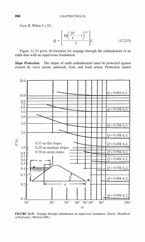
358 CHAPTER TWELVE
Case II. When I < 2U,
(12.213)
Figure 12.33 gives 10 formulas for seepage through the embankment of anearth dam with an impervious foundation.
Slope Protection. The slopes of earth embankments must be protected againsterosion by wave action, rainwash, frost, and wind action. Protection cannot
Q � � hk� 2U
I� 1�
1�3
2�L
20.0
10.0
8.07.06.05.0
4.0
3.0
2.0
1.00.33-m-flat slopes0.25-m-medium slopes0.10-m-steep slopes
m
ht
dht
0.80.70.60.50.4
0.3
0.2
0.110° 20° 30° 40° 50° 60° 80° 100°
Q = 0.90k ht L
Q = 0.80k ht L
Q = 0.70k ht L
Q = 0.60k ht L
Q = 0.50k ht L
Q = 0.40k ht L
Q = 0.30k ht L
Q = 0.20k ht L
Q = 0.10k ht L
Q = 0.05k ht L
d
α
α
FIGURE 12.33 Seepage through embankment on impervious foundation. (Davis—Handbookof Hydraulics, McGraw-Hill.)

HYDRAULICS AND WATERWORKS FORMULAS 359
economically by provided against the erosion which would occur if the dam wereovertopped. A major cause of earth-dam failures has been overtopping; therefore,care must be exercised that freeboard and spillway capacity are ample to prevent it.
Wave Action. The height and velocity of waves are functions of fetch and windvelocity. Fetch is the clear-water distance form the dam to the opposite shore.Generally the straight-line distance is used. However, where slight bends in themeasured line will lengthen the fetch, such bends may be incorporated accordingto judgment. The Molitor-Stevenson equation for the height of waves, hw, is
For a fetch greater than 20 miles,
(12.214)
For a fetch less than 20 miles,
(12.215)
where hw � height of wave from trough to crest, ftV � wind velocity, mphF � fetch, statute miles
For wave heights between 1 and 7 ft, the velocity, v, in feet per second isgiven approximately by the formula
(12.216)
where is in feet.
Freeboard. Freeboard (sometimes termed net freeboard) is the verticaldistance between the maximum water surface of the spillway design flood andthe crown of the dam. This vertical distance should be ample to preventovertopping of the dam due to wind setup and wave action.
Wind setup may be computed by the Zuider Zee formula
(12.217)
where S � setup above pool level, ftV � wind velocity, mphF � fetch, milesD � average depth of water, ftA � angle of incidence of waves
The height of waves above pool level plus the run-up of waves on the faceof the dam may be computed by the formula
Height of wave action (12.218)� 0.75hw �V2
2g1.5hw
S �V 2F
1,400Dcos A
hw
v � 7 � 2hw
hw � 0.17(VF)0.5 � 2.5 � (F)0.25
hw � 0.17(VF)0.5

This page intentionally left blank

CHAPTER 13
361
STORMWATER, SEWAGE,SANITARY WASTEWATER,
AND ENVIRONMENTALPROTECTION*
DETERMINING STORM WATER FLOW
Sewers must handle storm water flows during, and after, rain storms, and snow-and ice-melting events. The rational formula for peak storm-water runoff is
Q � CIA (13.1)
where Q � peak runoff, ft3/sA � drainage area, acresC � coefficient of runoff of areaI � average rainfall rate, in/h of rain producing runoff
In heavily populated urban areas C ranges from 0.70 to 0.90. Residential areaswith gardens, shrubs, and extensive open land have C values ranging from 0.30to 0.40.
FLOW VELOCITY IN STRAIGHT SEWERS
Obstruction-free straight sewers will have a flow velocity of
(13.2)V �C
nR2/3S1/2
*Hicks—Handbook of Civil Engineering Calculations, McGraw-Hill. The formulas and text in thischapter, beginning with formula 13.11 and running through 13.77, and 13.84 through 13.88, are thework of Kevin D. Wills, M.S.E., P.E., Consulting Engineer.

362 CHAPTER THIRTEEN
where n � coefficient dependent on roughness of conduit surfaceR � hydraulic radius, ft � area, ft2, of fluid divided by wetted perimeter, ftS � energy loss, ft/ft of conduit length; approximately the slope of the
conduit invert for uniform flowC � 1.486 (conversion factor to account for change from metric units
used in development of the formula)
The value of n can range from 0.013 in smooth concrete sewers to 0.02 in plainpipe. Further, n usually increases as a sewer pipe ages. Specific n values aregiven in engineering handbooks such as those cited in the references section ofthis book.
The water flow, cu ft/s is
Q � AV (13.3)
where A � cross-sectional area of flow, ft2.
Required Flow Velocity
To ensure full carriage of the solids, soils, refuse, and sand conveyed by stormand sanitary sewers, minimum flow velocities must be maintained. For stormsewers, the minimum flow velocity should be 3 ft/s; for sanitary sewers, 2 ft/sis recommended. Full-flow velocity of the liquid in a sewer is given by:
(13.4)
where d � inside diameter of pipe, ft.Flow quantity, cu ft/s, for a full-flowing sewer pipe is given by
(13.5)
Disposing of Storm Water
Storm water must be allowed to drain off streets and roads to prevent pond-ing and interference with pedestrian and vehicular traffic. Storm-waterinlets, Fig. 13.1, at a curb opening, with full gutter flow, have a capacity of:
(13.6)
where Q � quantity of runoff, ft3/sL � length of opening, fta � depression in curb inlet, fty � depth of flow at inlet, ft
Q � 0.7L (a � y)3/2
Q �0.463
nd8/3S1/2
V �0.59
nd2/3S1/2

STORMWATER, WASTEWATER, AND ENVIRONMENTAL PROTECTION 363
When a grate inlet is used to collect the storm water, an opening of 18 in, ormore, is recommended. With a flow depth of up to 4.8 in, the inlet capacity is
(13.7)
where P � perimeter, ft, of grate opening over which water may flow, ignoringthe bars.
If the flow depth exceeds 1 ft 5 in, the capacity is
(13.8)
where A � total area of clear opening, ft2
g � acceleration due to gravity, 32 ft/s2
Controlling Sewer-Water Flow
Controls used to regulate sewer-water flow include side weirs, siphon spill-ways, and leaping weirs (Fig. 13.2). Flow diversion for a side weir is, in cu ft/s:
(13.9)Q � 3.32l0.83h1.67
Q � 0.6A22gy
Q � 3Py3/2
Manhole coverJointfiller Curb
Normal gutter line
Depressedgutter
3' wide5'
Opening
Minimuminside
width 2'-6"
Rungs-14"C. to C.
Pipe
12 1
6"
6"
Invert shaped withconcrete fill
6"
FIGURE 13.1 Storm-water inlet with opening in a curb. (Merritt—Standard Handbook forCivil Engineering, McGraw-Hill.)

364 CHAPTER THIRTEEN
where l � length of weir, fth � depth of flow over weir at down-stream end, ft
Siphon spillways are better adapted to handling large storm water and sewerflows. The area for the siphon throat, A sq ft, is:
(13.10)
where Q � discharge, ft3/sc � coefficient of discharge, which varies from 0.6 to 0.8g � acceleration due to gravity � 32.2 ft/s2
h � head, ft
DESIGN OF A COMPLETE-MIX ACTIVATED SLUDGE REACTOR
The volume of the reactor can be determined using the following equationderived from Monod kinetics:
(13.11)Vr �� cQY(So � S)
Xa(1 � kd� c)
A �Q
c�2gh
Combined
sewerSiphon
Bypass
Combined
sewer
Storm
sewer Sewer
Air vent
Weir
(a) (b)
Wet-weather
flow
(c)
Sanitary
sewerStorm
sewer
FIGURE 13.2 Flow-regulating devices for sewers: (a) Side weir. (b) Siphon spillway.(c) Leaping weir. (Merritt—Standard Handbook for Civil Engineering, McGraw-Hill.)

STORMWATER, WASTEWATER, AND ENVIRONMENTAL PROTECTION 365
where Vr � reactor volume (Mgal) (m3)�c � mean cell residence time, or the average time that the sludge remains
in the reactor (sludge age). For a complete-mix activated sludgeprocess, �c ranges from 5 to 15 days. The design of the reactor isbased on �c on the assumption that substantially all the substrate(BOD) conversion occurs in the reactor.
Q � average daily influent flow rate (Mgd)Y � maximum yield coefficient (mg VSS/mg BOD5). For the activated
sludge process for domestic wastewater Y ranges from 0.4 to 0.8.Essentially, Y represents the maximum mg of cells produced per mgorganic matter removed.
S0 � influent substrate (BOD5) concentration (mg/L)S � effluent substrate (BOD5) concentration (mg/L)
Xa � concentration of microorganisms in reactor � mixed liquor volatilesuspended solids (MLVSS) in mg/L. It is generally accepted that theratio MLVSS/MLSS � 0.8, where MLSS is the mixed liquor sus-pended solids concentration in the reactor. MLSS represents the sumof volatile suspended solids (organics) and fixed suspended solids(inorganics). For a complete-mix activated sludge process, MLSSranges from 1000 to 6500 mg/L.
kd � endogenous decay coefficient (d–1) which is a coefficient represent-ing the decrease of cell mass in the MLVSS. The activated sludgeprocess for domestic wastewater kd ranges from 0.025 to 0.075 d–1.
The hydraulic retention time, �, is
� � Vr /Q (13.12)
For a complete-mix activated sludge process, (� is generally 3 to 5 h).The observed cell yield:
Yobs � Y/1 � kd�c (13.13)
And the observed cell yield is always less than the maximum cell yield, (Y).The increase in MLVSS is computed using the following equation:
(13.14)
where Px is the net waste activated sludge produced each day in (lb VSS/d).The theoretical oxygen requirements for the removal of the carbonaceous
organic matter in waste water for an activated-sludge system can be computedusing the following equation:
O2/d (lb) � (total mass of BODL utilized, lb/d)� 1.42 (mass of organisms wasted, lb/d) (13.15)
Using terms that have been defined previously where f � conversion factorfor converting BOD5 to BODL (0.68 is commonly used):
(13.16)O2/d(lb) �
Q(SO � S)�8.34lb/Mgal
mg/L �f
� (1.42)(Px)
Px � YobsQ (SO � S)(8.34 lb/Mgal/mg/L)

366 CHAPTER THIRTEEN
It is recommended that aeration equipment be designed with a factor ofsafety of at least 2.
The food to microorganism ratio is defined as
F:M � SO�Xa (13.17)
where F:M is the food to microorganism ratio in d–1.F:M is simply a ratio of the “food” or BOD5 of the incoming waste, to the
concentration of “microorganisms” in the aeration tank or MLVSS.Typical values for F:M reported in literature vary from 0.05 d–1 to 1.0 d–1
depending on the type of treatment process used.The volumetric (organic) loading (VL) is defined as
(13.18)
VL is a measure of the pounds of BOD5 applied daily per thousand cubic feetof aeration tank volume.
To determine the waste activated sludge (WAS) and return activated sludge(RAS), Figs. 13.3 and 13.4 are used, along with the following variables:
VL � SOQ/Vr � SO/�
Q, S0
X, S, Vr
Control volume
Aeration tank
Qr, xr, SReturn
line
Settlingtank
Qe, S, Xe
Qw, X
Q + QrX
FIGURE 13.3 Aeration tank mass balance. (Hicks—Handbook of CivilEngineering Calculations, McGraw-Hill.)
Settlingtank
Q, So
X, S, Vr
Aeration tank
Qr, Xr, S
Qw, Xr
Return line
Qe, S, XeQ + QrX
Control volume
FIGURE 13.4 Settling tank mass balance. (Hicks—Handbook of Civil EngineeringCalculations, McGraw-Hill.)

STORMWATER, WASTEWATER, AND ENVIRONMENTAL PROTECTION 367
X � mixed liquor suspended solids (MLSS)
Qr � return activated sludge pumping rate (Mgd)
Xr � concentration of sludge in the return line (mg/L). When lacking sitespecific operational data, a value commonly assumed is 8000 mg/L.
Qe � effluent flow rate (Mgd)
Xe � concentration of solids in effluent (mg/L). When lacking site specificoperational data, this value is commonly assumed to be zero.
Qw � waste activated sludge (WAS) pumping rate from the reactor (Mgd)
Qw� � waste activated sludge (WAS) pumping rate from the return line (Mgd)
Other variables are as defined previously.
(a) Waste Activated Sludge (WAS) pumping rate from the return line. If the meancell residence time is used for process control and the wasting is from the sludgereturn line (Fig. 13.3), the wasting rate is computed using the following:
(13.19)
Assuming that the concentration of solids in the effluent from the settlingtank (Xe) is low, then the above equation reduces to:
(13.20)
To determine the WAS pumping rate using this method, the solids concen-tration in both the aeration tank and the return line must be known.
If the food to microorganism ratio (F:M) method of control is used, theWAS pumping rate from the return line is determined using the following:
(13.21)
(b) Waste Activated Sludge (WAS) pumping rate from the aeration tank. If themean cell residence time is used for process control, wasting is from the aer-ation tank (Fig. 13.4 and the solids in the plant effluent (Xe) are againneglected, then the WAS pumping rate is estimated using the following:
(13.22)
Assuming that the sludge blanket level in the settling tank remains constantand that the solids in the effluent from the settling tank (Xe) are negligible, amass balance around the settling tank (Fig. 13.3) yields the following equationfor RAS pumping rate:
(13.23)Qr �XQ � XrQw�
Xr � X
�c �Vr
Qw
Qw �Vr
� c
Px(ss) � Qw�Xr(8.34 lb/Mgal/mg/L)
� c �Vr X
Qw�Xr
Qw� �Vr X
� cXr
� c �Vr X
(Qw�Xr � QeXe)

368 CHAPTER THIRTEEN
The ratio of RAS pumping rate to influent flow rate, or recirculation ratio (�),may now be calculated:
(13.24)
Recirculation ratio can vary from 0.25 to 1.50 depending upon the type ofactivated sludge process used. Common design practice is to size the RASpumps so that they are capable of providing a recirculation ratio ranging from0.50 to 1.50.
DESIGN OF A CIRCULAR SETTLING TANK
Circular settling tanks are widely used in domestic wastewater treatment. Sur-face loading rates for settling tanks should be based on the peak flow conditionanticipated, using a peaking factor to adjust for unanticipated overloads. Or,
Qp � (average daily load, Mgd) (peaking factor) (13.25)
A peaking factor of 2.0 to 4.0 might be chosen by a designer based on the prob-able load on the system.
The surface area of the settling tank is
A � Qp /(design surface loading rate, gal/day/sq ft) (13.26)
The toal solids load on a clarifier consists of loads from the influent and theReturn Activated Sludge (RAS). Then:
Qr � RAS flow rate � 1.25 (Q) (13.27)
X � MLSS in aeration tank
Therefore, the maximum solids loading occurs at peak flow and maximumRAS flow rate. The maximum solids entering the clarifier is calculated using:
Max solids (lb/d) � (Qp � Qr)(X)(8.34) lb�L/mg�Mgal) (13.28)
The surface area needed, based on an assumed solids loading rate (such as2.0 (lb/sq�ft�h) at peak flow) is
A � (maximum solids)/(assumed solids loading rate) (13.29)
Since two required areas have been computed, designers choose the largerof the two areas to provide safety in the design. For backup purposes two tanksare normally chosen. The actual solids loading can be compared with theassumed loading using
A � (solids processed, lb/h)/(total settling tank surface area, sq ft) (13.30)
α �Qr
Q

STORMWATER, WASTEWATER, AND ENVIRONMENTAL PROTECTION 369
SIZING A POLYMER DILUTION/FEED SYSTEM
Depending on the quality of settled secondary effluent, organic polymer addi-tion is often used to enhance the performance of tertiary effluent filters in adirect filtration process: see Design of a Rapid Mix Basin and FlocculationBasin. Because the chemistry of the wastewater has a significant effect on theperformance of a polymer, the selection of a type of polymer for use as a filteraid generally requires experimental testing. Common test procedures for poly-mers involve adding an initial polymer dosage to the wastewater (usually 1 partper million, ppm) of a given polymer and observing the effects. Dependingupon the effects observed, the polymer dosage should be increased or decreasedby 0.5 ppm increments to obtain an operating range.
The gallons per day (gal/day) (L/d) of active polymer required is calculatedusing the following:
Active polymer (gal/day) � (wastewater flow, Mgd) � (active polymer dosage, ppm) (13.31)
The quantity of dilution water required is calculated using the following:
(13.32)
The quantity of neat polymer required is calculated as follows:
(13.33)
(13.34)
DESIGN OF A SOLID-BOWL CENTRIFUGE FOR SLUDGE DEWATERING
Centrifuges are commonly used for thickening or dewatering Waste ActivatedSludge (WAS) and other biological sludges from secondary wastewater treat-ment. In the process, centrifuges reduce the volume of stabilized (digested)sludges to minimize the cost of ultimate disposal.
The capacity of sludge dewatering to be installed at a given facility is afunction of the size of a facility, capability to repair machinery on-site, and theavailability of an alternative disposal means. Some general guidelines relatingthe minimal capacity requirements are listed in Table 13.1 This table is basedon the assumption that there is no alternative mode of sludge disposal and thatthe capacity of store solids is limited.
Time required to use one drum of polymer �drum capacity, gal
neat polymer, gal/h
Neat polymer (gal/h) �active polymer, gal/h
% active polymer in emulsion as supplied
Dilution water (gal/h) �active polymer, gal/h
% solution used (as a decimal)

370 CHAPTER THIRTEEN
The sludge feed rate for the dewatering facility is
(13.35)
And the sludge weight flow rate is
(13.36)
Ws � weight flow rate of sludge feed, lb/h (kg/h)
V � volume flow rate of sludge feed, gal/min (L/s)
s.g. � specific gravity of sludge
% solids � percent solids expressed as a decimal
� � density of water, 62.4 lb/ft3 (994.6 kg/m3)
Since the solids exiting the centrifuge are split between the centrate and thecake, it is necessary to use a recovery formula to determine solids capture.Recovery is the mass of solids in the cake divided by the mass of solids in thefeed. If the solids content of the feed, centrate, and cake are measured, it is pos-sible to calculate percent recovery without determining total mass of any of thestreams. The equation for percent solids recovery is
(13.37)
where R � recovery, percent solidsCs � cake solids, percent solids (25%)F � feed solids, percent solids (5%)
Cc � centrate solids, percent solids (0.3%)
The dewatered sludge (cake) discharge rate is
Cake discharge rate (lb/h) dry solids � (sludge feed rate, lb/h)(solids recovery)(13.38)
R � 100� Cs
F �� F � Cc
Cs � Cc�
Ws �(V)(p)(s.g.)(% solids)(60 min/h)
7.48 gal/ft3
Sludge feed rate �gal/day of digested sludge
operating h/day, 7 days/week (60 min/h)
TABLE 13.1 Facility Capacity and Number of Centrifuges
Facility size, Dewatering Centrifuges operating �Mgd (m3/d) operation, h/d Spare @ gal/min (L/s)
2 (7570) 7 1 � 1 @ 25 (1.58)5 (18,930) 7.5 1 � 1 @ 50 (3.16)20 (75,700) 15 2 � 1 @ 50 (3.16)50 (189,250) 22 2 � 1 @ 75 (4.73)100 (378,500) 22 3 � 2 @ 100 (6.31)250 (946,250) 22 4 � 2 @ 200 (12.62)
(Design Manual for Dewatering Municipal Wastewater Sludges, U.S. EPA)

STORMWATER, WASTEWATER, AND ENVIRONMENTAL PROTECTION 371
The wet cake discharge (lb/h) is
(13.39)
The volume of wet cake, assuming a cake density of 60 lb/ft3 is
(13.40)
The percent reduction in sludge volume is then
(13.41)
The centrifugal acceleration force (G), defined as multiples of gravity, is afunction of the rotational speed of the bowl and the distance of the particle fromthe axis of rotation. In the centrifuge, the centrifugal force, G, is calculated asfollows:
(13.42)
where N � rotational speed of centrifuge (rev/s)R � bowl radius, ft (cm)
The polymer feed rate (lb/h) of dry polymer is
(13.43)
Polymer feed rate (gal/h) is
(13.44)
where s.g. � specific gravity of the polymer solution % polymer concentration expressed as a decimal
DESIGN OF A TRICKLING FILTER USING THE NRC EQUATIONS
Two possible process flow schematics for a two-stage trickling filter system areshown in Fig. 13.5.
Polymer feed rate (gal/h) �polymer feed rate (lb/h)
(8.34 lb/gal)(s.g.)(% polymer concentration)
Polymer feed rate (lb/h) �(polymer dosage, lb/ton)(dry sludge feed, lb/h)
2000 lb/ton
G �(2 N)2R
32.2 ft/s2
% Volume reduction �sludge volume in � sludge volume out
sludge volume in
Volume of wet cake (ft3/h) �wet cake rate, lb/h
cake density, lb/ft3
Wet cake discharge (lb/h) �dry cake rate, lb/h
cake % solids

372 CHAPTER THIRTEEN
The NRC equations for trickling filter performance are empirical equations,which are primarily applicable to single and multistage rock systems with recir-culation.
The overall efficiency of the two-stage trickling filter is
(13.45)
Also, overall efficiency � E1 � E2(1 – E1); and E1 � E2. (13.46)
where E1 � the efficiency of the first filter stage, including recirculation and set-tling (%)
E2 � the efficiency of the second filter stage, including recirculation andsettling (%)
For a single stage or first stage rock trickling filter, the NRC equation is
(13.47)
where W � BOD5 loading to the filter, lb/d (kg/d)V � volume of the filter media, 103 ft3 (m3)F � recirculation factor
Recirculation factor represents the average number of passes of the influentorganic matter through the trickling filter. The recirculation factor is
(13.48)F �1 � R
[1 � (R�10)]2
E1 �100
1 � 0.0561BW
VF
Overall efficiency �influent BOD5 � effluent BOD5
influent BOD5� 100
FIGURE 13.5 Two-stage trickling filter process flow schematics. (Hicks—Handbook ofCivil Engineering Calculations, McGraw-Hill.)
Recycle
Influent
Influent
Primaryclarifier
Primaryclarifier
First-stagefilter
First-stagefilter
Recycle Recycle
EffluentClarifier
Second-stagefilter
Second-stagefilter
Clarifier
ClarifierEffluent
Recycle

STORMWATER, WASTEWATER, AND ENVIRONMENTAL PROTECTION 373
where R � recirculation ratio � Qr /QQr � recirculation flowQ � wastewater flow
The BOD5 loading for the first stage filter is calculated using
W � (influent BOD5, mg/L)(wastewater flow, Mgd)\ � (8.34 lb/Mgal/mg/L) (13.49)
The BOD5 loading for the second stage trickling filter is
(13.50)
where loading to the second stage filter.The NRC equation for a second stage trickling filter is
(13.51)
The hydraulic loading to each filter is
(13.52)
DESIGN OF A RAPID-MIX BASIN AND FLOCCULATION BASIN
The hydraulic retention time of typical rapid mix operations in wastewatertreatment range from 5 to 20 seconds. The required volume of the rapid-mixbasin, Fig. 13.6, is
Volume (V) � (hydraulic retention time)(wastewater flow)
Hydraulic loading �(1 � R)(Q)
(area)(1440 min/d)
E2 �100
1 �0.0561
1 � E1BW�
VF
W� � BOD5
W� � (1 � E1)W
FIGURE 13.6 Process flow for direct filtration. (Hicks—Handbook of Civil EngineeringCalculations, McGraw-Hill.)
To
disinfection
FiltrationFlocculationRapid mix
(coagulation)
From
secondary
treatment
Polymer
addition

374 CHAPTER THIRTEEN
The power input per volume of liquid is generally used as a rough measureof mixing effectiveness, based on the reasoning that more input power createsgreater turbulence, and greater turbulence leads to better mixing. The followingequation is used to calculate the required power for mixing:
(13.53)
where G � mean velocity gradient (s–1)P � power requirement (ft�lb/s) (kW)� � dynamic viscosity (lb�sq ft) (Pa�s)V � volume of mixing tank (ft3) (m3)
G is a measure of the mean velocity gradient in the fluid. G values for rapidmixing operations in wastewater treatment range from 250 to 1500 s–1.
The required power for mixing is
P � G2�V (13.54)
The required volume of the flocculation basin is
(13.55)
G values for flocculation in a direct filtration process range from 20 to 100 s–1.The power required for flocculation is
(13.56)
If the flows to the rapid mix and flocculation basin vary significantly, orturn down capability is desired, a variable speed drive should be provided foreach mixer and flocculator.
It should be noted that the above analysis provides only approximate valuesfor mixer and flocculator sizes. Mixing is in general a “black art,” and a mixingmanufacturer is usually consulted regarding the best type and size of mixer orflocculator for a perticular application.
DESIGN OF AN AEROBIC DIGESTER
The volume of digested sludge is
(13.57)
where V � sludge volume (ft3) (m3)Ws � weight of sludge (lb) (kg)
� � density of water (62.4 lb/ft3) (994.6 kg/m3)s.g. � specific gravity of digested sludge (assume s.g. � 1.03)
% solids � percent solids expressed as a decimal
V �Ws
(ρ)(s.g.)(% solids)
P � G2�V
V �(retention time, min) (flow rate of secondary effluent, Mgd)
(min per day)
G � BP
�V

STORMWATER, WASTEWATER, AND ENVIRONMENTAL PROTECTION 375
The weight of oxygen, (lb2/day) required to destroy the VSS is approximately
(13.58)
Then, the volume of air required at standard conditions of 14.7 lb/sq in and68 F with 23.2 percent oxygen by weight and a density of 0.075 lb/ft3 is:
(13.59)
The volume of the aerobic digester is computed using the following equa-tion, assuming the digester is loaded with waste activated sludge only:
(13.60)
where V � volume of aerobic digester, ft3 (m3)Qi � influent average flow rate to the digester, ft3/d (m3/d)Xi � influent suspended solids, mg/L (50,000 mg/L for 5.0% solids)X � digester total suspended solids, mg/L
Kd � reaction rate constant, d–1. May range from 0.05 d–1 at 15°C (59°F)to 0.14 d–1 at 25°C (77°F)
Pv � volatile fraction of digester suspended solids (expressed as a decimal)� � solids retention time (sludge age), d
The usual design procedure computes needed values for both summer andwinter conditions for the digester.
DESIGN OF A PLASTIC MEDIA TRICKLING FILTER
Due to the predictable properties of plastic media, empirical relationships areavailable to predict performance of trickling filters packed with plastic media.However, the treatability constant must first be adjusted for both the tempera-ture of the wastewater and the depth of the actual filter.
Adjustment for temperature. The treatability constant is first adjusted fromthe given standard at 20°C (68°F) to the actual wastewater temperature using
(13.61)
where k30/20 � treatability constant at 30°C (86°F) and 20 ft (6.1 m) filter depthk20/20 � treatability constant at 20°C (68°F) and 20 ft (6.1 m) filter depth
(as example values)� � temperature activity coefficient (assume 1.035)T � wastewater temperature
Note: The actual temperature, °C and depth, ft (m) are used when this for-mula is applied in practice. The numbers given here are for illustrative purposesonly.
k30�20 � k20�20�T�20
V �QiXi
X(KdPv � 1� c)
Volume of air (ft3) � (WO2)�(0.075 lb/ft3) (0.232)
WO2� (lb VSS/d) (2.3 lb O2/lb VSS)

376 CHAPTER THIRTEEN
Adjustment for depth. The treatability constant is then adjusted from thestandard depth of 20 ft (6.1 m) to the example filter depth of 25 ft (7.6 m) usingthe following equation:
(13.62)
where k30/25 � treatability constant at 30°C (86°F) and 25 ft (7.6 m) filter depth(as example value)
k30/20 � treatability constant at 30°C (86°F) and 20 ft (6.1 m) filter depthD1 � depth of reference filter (20 ft) (6.1 m)D2 � depth of actual filter (25 ft) (7.6 m) (as example value)
x � empirical constant (0.3 for plastic medium filters)
The empirical formula used for sizing plastic media trickling filters is
(13.63)
where Se � BOD5 of settled effluent from trickling filter (mg/L)Si � BOD5 of influent wastewater to trickling filter (mg/L)
k20 � treatability constant adjusted for wastewater temperature and filterdepth � (k30/25)
D � depth of filter (ft)Qv � volumetric flowrate applied per unit of filter area (gal/min�sq ft)
(L/s�m2) � Q/AQ � flowrate applied to filter without recirculation (gal/min)(L/s)A � area of filter (sq�ft) (m2)n � empirical constant (usually 0.5)
Rearranging and solving for the trickling filter area (A):
(13.64)
The hydraulic loading of the filter in gpm/ft2, or L/s�m2 is
Hydraulic loading � Q/A (13.65)
For plastic media trickling filters, the hydraulic loading ranges from 0.2 to1.20 gal/min�sq�ft (0.14 to 0.82 L/s�m2).
The organic loading to the trickling filter is calculated by dividing the BOD5load to the filter by the filter volume as follows:
Organic loading � BOD5/(A) (filter length, ft) (13.66)
For plastic media trickling filters, the organic loading ranges from 30 to200 lb/103 ft3�d (146.6 to 977.4 kg/m2�d).
To optimize the treatment performance of a trickling filter, there should be acontinual and uniform growth of biomass and sloughing of excess biomass; to
A � Q� �ln(Se/Si
(k30/25)D�
1/n
Se
Si
� exp[�kD(Qv)�n]
k30/25 � k30/20(D1/D2)x

STORMWATER, WASTEWATER, AND ENVIRONMENTAL PROTECTION 377
achieve uniform growth and sloughing, higher periodic dosing rates arerequired. The required dosing rate in inches per pass of distributor arm may beapproximated using the following:
Dosing rate � (organic loading, lb/103 ft3�d)(0.12) (13.67)
Typical dosing rates for trickling filters are listed in Table 13.2. To achievethe typical dosing rates, the speed of the rotary distributor can be controlled by(1) reversing the location of some of the existing orifices to the front of the dis-tributor arm, (2) adding reversed deflectors to the existing orifice discharges,and (3) by operating the rotary distributor with a variable speed drive.
The rotational speed of the distributor is a function of the instantaneous dos-ing rate and may be determined using the following:
(13.68)
where n � rotational speed of distribution (rpm)QT � total applied hydraulic loading rate (gal/min�sq ft) (L/s�m2) �
Q � QRQ � influent wastewater hydraulic loading rate (gal/min�sq ft) (L/s�m2)
QR � recycle flow hydraulic loading rate (gal/min�sq ft) (L/s�m2) Note:recycle is assumed to be zero in this example.
A � number of arms in rotary distributor assemblyDR � dosing rate (in/pass of distributor arm)
DESIGN OF AN ANAEROBIC DIGESTOR
Anaerobic digestion is one of the oldest processes used for the stabilization ofsludge. It involves the decomposition of organic and inorganic matter in theabsence of molecular oxygen. The major applications of this process are in thestabilization of concentrated sludges produced from the treatment of wastewater.
n �1.6(QT)
(A)(DR)
TABLE 13.2 Typical Dosing Rates for Trickling Filters
Organic loading lb BOD5/103 Dosing rate,ft3�d (kg/m2�d) in./pass (cm/pass)
<25 (122.2) 3 (7.6)50 (244.3) 6 (15.2)75 (366.5) 9 (22.9)100 (488.7) 12 (30.5)150 (733.0) 18 (45.7)200 (977.4) 24 (60.9)
(Wastewater Engineering: Treatment, Disposal, and Reuse, Metcalf& Eddy, 3rd Ed, McGraw-Hill.)

378 CHAPTER THIRTEEN
In the anaerobic digestion process, the organic material is converted biologi-cally, under anaerobic conditions, to a variety of end products includingmethane (CH4) and carbon dioxide (CO2). The process is carried out in an air-tight reactor. Sludge, introduced continuously or intermittently, is retained inthe reactor for varying periods of time. The stabilized sludge, withdrawn con-tinuously or intermittently from the reactor, is reduced in organic and pathogencontent and is nonputrescible.
In the high rate digestion process, as shown in Fig. 13.7, the contents of thedigester are heated and completely mixed. For a complete-mix flow throughdigester, the mean cell residence time (�c) is the same as the hydraulic retentiontime (�).
The digester volume V required is
V � �cQ (13.69)
where V � required volume, ft3 (m3)�c � required hydraulic retention time, minQ � influent sludge flow rate, gal/day (m3/day)
Then, the
Volumetric loading � (BOD/day)/V (13.70)
The volumetric loading is expressed in lb/ft3 ( day�kg/m3�day).For high rate digesters, loading range from 0.10 to 0.35 lb/ft3�d (1.6 to 5.61
kg/m3�d).The quantity of volatile solids produced each day is
(13.71)Px �Y [(BODin, lb/d) � (BODout, lb/d)]
1 � kd� c
Fixed cover
Sludgeoutlets
Sludgeinlets
Sludge heater
Gas storage
Methane + Carbon dioxide
Mixer
FIGURE 13.7 High-rate single-stage complete-mix anaerobic digester. (Adapted fromMetcalf & Eddy, Wastewater Engineering: Treatment, Disposal, and Reuse, 3rd ed.,McGraw-Hill.)

STORMWATER, WASTEWATER, AND ENVIRONMENTAL PROTECTION 379
where Px � volatile solids produced, lb/d (kg/d)Y � yield coefficient (lb VSS/lb BODL)kd � endogenous coefficient (d–1)�c � mean cell residence time (d)
The volume of methane gas produced at standard conditions (32°F and 1 atm)(0°C and 101.3 kPa) is calculated using
(13.72)
where � volume of methane gas produced at standard conditions (ft3/d) (m3/d).
Percent stabilization is calculated using
(13.73)
DESIGN OF A CHLORINATION SYSTEM FOR WASTEWATER DISINFECTION
The reduction of coliform organisms in treated effluent is defined by
(13.74)
where Nt � number of coliform organisms at time tN0 � number of coliform organisms at time t0Ct � total chlorine residual at time t (mg/L)
t � residence time (min)
The required residual, RR is
(13.75)
Codes often require a residence time, t, of 15 min. However, the local codeshould be checked to determine the exact residence time currently required.
The capacity of the chlorinator at peak flow
Cl2 (lb/d) � (Dosage, mg/L)(Avg flow, Mgd)(P.F.)(8.34) (13.76)
where Cl2 � pounds of chlorine required per day (kg/d)Dosage � dosage used to obtain coliform reduction
Avg. Flow � average flowP.F. � peaking factor for average flow8.34 � 8.34 lb.L/Mgal.mg
RR � Ctt/t
Nt
N0� (1 � 0.23Ctt)�3
% Stabilization �[(BODin, lb/d) � (BODout, lb/d) � 1.42 Px]
BODin, lb/d� 100
VCH4
VCH4� 5.62 ft3/lb[(BODin, lb/d) � (BODout, lb/d) � 1.42Px]

380 CHAPTER THIRTEEN
The average daily consumption of chlorine is
Cl2 lb/d � (average dosage, mg/L) (Mgd)(8.34) (13.77)
A typical chlorination flow diagram is shown in Fig. 13.8. This is a com-pound loop system, which means the chlorine dosage is controlled through sig-nals received from both effluent flow rate and chlorine residual.
SANITARY SEWER SYSTEM DESIGN
Compute the sanitary sewer system flow rate, SSfr, gal/day:
SSfr � (city or town area, ac) (residential population/ac) � (gal/day of sewage per person) (13.78)
The residential population per acre (ac) can be determined from census dataor from data in engineering handbooks.
Convert SSfr from gal/day to cubic feet per second, cfs with
cfs � 1.55 (gpd/106) (13.79)
Size the main sewer, into which lateral sewers discharge, on the basis offlowing full. This is the usual design procedure followed by experienced sani-tary engineers.
Flow meterInjector
Chlorine gas
Control signal
Chlorinator
Compressedgas storageControl
signalChlorine residualanalyzer
Receiving water or reuse
Chlorine solution
Chlorinecontactchannel
Rotometer
Watereffluent
FIGURE 13.8 Compound-loop chlorination system flow diagram. (Hicks—Handbook ofCivil Engineering Calculation, McGraw-Hill.)

STORMWATER, WASTEWATER, AND ENVIRONMENTAL PROTECTION 381
To size the main and lateral sewers, use the Manning formula and the appro-priate conveyance factor from Table 13.2.
When the conveyance factor Cf is used, the Manning formula becomes
(13.80)
where Q � flow rate through the pipe, ft3/s; Cf � conveyance factor corre-sponding to a specific n value listed in Table 13.3; S � pipe slope or hydraulicgradient, ft/ft.
Next, compute the flow rate for each lateral sewer discharging into the mainsewer using
LSfr � (SSfr)/(percent lateral sewer flow, expressed as a whole number)(13.81)
In this formula, SSfr is expressed in cfs, as computed earlier.Compute the lateral sewer pipe diameter using the Manning formula, as given
above. Next, compute the value of for each lateral sewer pipe in the system.Then take the sum of all lateral pipes, or
(13.82)
The ΣLS should be less than d2.5 for the main sewer. If the ΣLS is greater thanthe d2.5 for the main sewer, the diameter of the main sewer should be increaseduntil its d2.5 is greater than ΣLS.
Next, compute the sewer size with infiltration from the groundwater. Infil-tration is the groundwater that enters a sewer. The quantity and rate of infiltra-tion depend on the character of the soil in which the sewer is laid, the relativeposition of the groundwater level and the sewer, the diameter and length of thesewer, and the material and care with the sewer is constructed. With tile andother joined sewers, infiltration depends largely on the type of joint used in thepipes. In large concrete or brick sewers, the infiltration depends on the type ofwaterproofing applied.
LS� d2.5
LS1 � d2.5LS2 . . ..
d2.5LS
Q � Cf S1/2
TABLE 13.3 Manning Formula Conveyance Factor
Pipe Pipe diameter, cross-sectional
n
in (mm) area, sq ft (m2) 0.011 0.013 0.015 0.017
6 (152) 0.196 (0.02) 6.62 5.60 4.85 4.288 (203) 0.349 (0.03) 14.32 12.12 10.50 9.27
10 (254) 0.545 (0.05) 25.80 21.83 18.92 16.7012 (305) 0.785 (0.07) 42.15 35.66 30.91 27.2715 (381) 1.227 (0.11) 76.46 64.70 56.07 49.4818 (457) 1.767 (0.16) 124.2 105.1 91.04 80.3321 (533) 2.405 (0.22) 187.1 158.3 137.2 121.1

382 CHAPTER THIRTEEN
Infiltration is usually expressed in gallons per day per mile of sewer. Withvery careful construction, infiltration can be kept down to 5000 gal/(day�mi)[0.14 L/(km�s)] of pipe even when the groundwater level is above the pipe.With poor construction, porous soil, and high groundwater level, infiltrationmay amount to 100,000 gal/(day�mi) [2.7 L/(km�s)] or more. Sewers laid indense soil where the groundwater level is below the sewer do not experienceinfiltration except during and immediately after a rainfall. Even then, the infil-tration will be small amounts.
The total infiltration to a sanitary sewer system is
Ti (gpd) � (infiltration, gpd/mi) (sewer system length, mi) (13.83)
Compute the infiltration for each lateral sewer and add it to the infiltrationinto the main sewer. The capacity of the main sewer must be such that it canhandle the sanitary sewage load plus the infiltration load. If the main sewer istoo small to handle both the loads, it must be enlarged, using the Manning for-mula, to handle both the loads with some reserve capacity.
Where a sewer must also handle the runoff from fire-fighting apparatus,compute the quantity of fire-fighting water for cities of less than 200,000 populationfrom where Q � fire demand, gal/min; and P �city population in thousands. Add the fire demand to the sanitary sewageand infiltration flows to determine the maximum quantity of liquid the sewermust handle. For cities having a population of more than 200,000 persons,consult the fire department headquarters to determine the water flow quanti-ties anticipated.
Some sanitary engineers apply a demand factor to the average daily waterrequirements per capita before computing the flow rate into the sewer. Thus,the maximum monthly water consumption is generally about 125 percent of theaverage annual demand but may range up to 200 percent of the average annualdemand. Maximum daily demands of 150 percent of the average annual demandand maximum hourly demands of 200 to 250 percent of the annual averagedemand are commonly used for design by some sanitary engineers.
Most local laws and many sewer authorities recommend that no sewer beless than 8 in (203 mm) in diameter. The sewer should be sloped sufficiently togive a flow velocity of 2 ft/s (0.6 m/s) or more when flowing full. This velocityprevents the deposit of solids in the pipe. Manholes serving sewers should notbe more than 400 ft (121.9 m) apart.
Where industrial sewage is discharged into a sanitary sewer, the industrialflow quantity must be added to the domestic sewage flow quantity before thepipe size is chosen. Swimming pools may also be drained into sanitary sewersand may cause temporary overflowing because the sewer capacity is inade-quate. The sanitary sewage flow rate from an industrial area may be less thanfrom a residential area of the same size because the industrial population issmaller.
Many localities and cities restrict the quantity of commercial and industrialsewage that may be discharged into public sewers. Thus, one city restricts com-mercial sewage from stores, garages, beauty salons, etc., to 135 gal/day percapita. Another city restricts industrial sewage from factories and plants to50,000 gal/(day�acre) [0.55 mL/(m�s)].
Q � 1020(P)0.5[1 � 0.01(P)0.5],

STORMWATER, WASTEWATER, AND ENVIRONMENTAL PROTECTION 383
DESIGN OF AN AERATED GRIT CHAMBER
Grit removal in a wastewater treatment facility prevents unnecessary abrasionand wear of mechanical equipment such as pumps and scrappers, and grit depo-sition in pipelines and channels. Grit chambers are designed to remove grit(generally characterized as non-putrescible solids) consisting of sand, gravel, orother heavy solid materials that have settling velocities greater than those of theorganic putrescible solids in the wastewater.
In aerated grit chamber systems, air introduced along one side near the bot-tom causes a spiral roll velocity pattern perpendicular to the flow through thetank. Figure 13.9 shows a typical aerated grit chamber.
At peak flow rate, the detention time in the aerated grit chamber shouldrange from 2 to 5 min. Because it is necessary to drain the chamber periodicallyfor routine maintenance, two redundant chambers are required. Therefore, thevolume of each chamber is
(13.84)
Width-depth ratio for aerated grit chambers range from 1:1 to 5:1. Depthsrange from 7 to 16 ft (2.1 to 4.87 m).
Width of grit chamber (ft) � (selected width-ratio) (chosen depth, ft)
V (ft3) �(peak flow rate, gal/day)(detention time, min)
(7.48 gal/ft3)(24 h/d)(60 min/h)
Inlet
Trajectory ofgrit particles
Outlet weir
Helical liquidflow pattern
FIGURE 13.9 Aerated grit chamber. (Metcalf & Eddy, WastewaterEngineering: Treatment, Disposal, and Reuse, 3rd ed., McGraw-Hill.)

384 CHAPTER THIRTEEN
Length of grit chamber (ft) � (volume)/[(width, ft) (depth, ft)] (13.86)
Length-width ratios range from 3:1 to 5:1.The air supply requirement for an aerated grit chamber ranges from 2.0 to
5.0 ft3/min/ft of chamber length (0.185 to 0.46 m3/min � m).
(13.87)
Grit quantities must be estimated to allow sizing of grit handling equipmentsuch as grit conveyors and grit dewatering equipment. Grit quantities from anaerated grit chamber vary from 0.5 to 27 ft3/Mgal (3.74 to 201.9 m3/L) of flow.
Volume of grit (ft3/day) � (assumed grit quantity, ft3/Mgal)� (Mgd handled) (13.88)
Air supply required (ft3/min) �(chosen air supply, ft3/min/ft)
chamber length, ft

INDEX

This page intentionally left blank
387
Activated sludge reactor, design of,364
Adjustment factors for lumber, 169
Aerated grit chamber, design of, 383
Aerobic digester, design of, 374Allowable bond stresses in concrete
beams, 124Allowable loads for piles, 105Allowable stress design for buildings,
208Aluminum columns, design loads
for, 96Anaerobic digester, design of,
377Anderson formula, 200Aquifers, 334Arch dams, 350Axial capacity of a single pile,
112Axially loaded steel columns, 102
Balanced reinforcing of concrete, 131
Beam formulas, 11–79beams of uniform strength, 52characteristics of loadings, 43column formulas, 250–253combined axial and bending loads,
72continuous beams, 11, 39, 40
Beam formulas (Cont.):curved beams, 65–69
eccentrically curved, 68eccentric loading, 73–74elastic diagrams, 21–31elastic-curve equations for
prismatic beams, 32–38elastic lateral buckling,
69–72fixed-end moments, 78natural circular and periods of
vibration, 74–76rolling and moving loads,
53–65safe loads for beams of various
types, 53–63Castigliano’s theorem, 52Maxwell’s theorem, 51parabolic beam, 52steel beam, 62triangular beam, 52
ultimate strength ofcontinuous beams, 46–52
uniform strength, 52unsymmetrical bending, 73
Blasting, vibration control in, 204Bridge and suspension-cable
formulas, 249–274allowable-stress design, 250
for bridge beams, 254for bridge columns, 250–254for shear, 249, 262

388 INDEX
Bridge and suspension-cable formulas(Cont.):
bearing on milled surfaces, 258bridge fasteners, 258cable systems, 272–273composite construction in highway
bridges, 259bending stresses, 260effective width of slabs, 259shear range, 260span/depth ratios, 259
connectors, number of, 261general relations for suspension
cables, 269–270keeping strength at different
levels, 269-270parabola, 268supports at different levels,
269–270supports at same level,
270–272hybrid bridge girders, 256load-and-resistance factor design,
250for bridge beams, 256for bridge columns, 250
maximum width/thickness ratios,263
number of connectors in bridges,261
ultimate strength of connectors,262
rainwater accumulation on, 273
shear strength design for bridges,249
stiffeners on bridge girders, 255
longitudinal stiffeners, 255suspension cables,
263–273catenary cable sag, 266parabolic cable tension and
length, 263–266
Building and structures formulas,207–248
allowable-stress design, 208for building beams,
209–211for building columns, 208for shear in buildings, 214
bearing plates, 216bents and shear in walls, 220
deflections of, 220choosing most economic structural
steel, 239carbon content, 240–241
column base plates, 217combined axial compression or
tension and bending, 221composite construction, 225connectors, 226–228design of stiffeners under load, 224fasteners in buildings, 225lightweight steel construction,
228–239load-and-resistance factor design,
207for building beams, 211–214for columns, 209for shear, 207
milled surfaces, bearing on, 218number of connections required,
226shear on connectors, 227
plate girders in buildings, 219ponding considerations, 228roof live loads, 244seismic loads, 246snow loads, 245statically indeterminate forces, 241stiffeners, 224stresses in thin shells, 215webs under concentrated loads,
222–224wind loads, 245
Buttress dams, 353foundations for, 354–356

INDEX 389
Cable systems, 272–273California bearing ratio, 195Cantilever retaining walls,
153–155Centrifugal pumps, 342–343Chezy formula, 302Chlorination system, design of 379Circular channels, 328Circular curves, 275Circular settling tank, design of,
368Column formulas, 81–104
for bridges, 249–254Column moments, 146Columns, axially loaded steel, 102Columns, lumber, 160Columns, of special metal materials,
88Commonly used USCS and SI units,
2Complete-mix activated sludge
reactor, 364Composite construction, 225Concrete, formulas for,
115–155braced and unbraced frames, 147cantilever retaining walls,
153–155column moments, 146compression development lengths,
128continuous beams, 11, 39, 46,
117–123one-way slabs, 117
crack control, 128deflection, computation for, 130design methods, 118
beams, 118–123columns, 123–127
flat-plate construction, 142direct design method, 144
flat-slab construction, 142footings, wall, 155gravity retaining walls, 150–153
Concrete, formulas for (Cont.):hardened-state properties, 127job mix volume, 116load-bearing walls, 148modulus of elasticity, 116properties in hardened state, 127reinforced, 115reinforcing steel, 117required strength, 129retaining walls, 150–155shear in slabs, 145shear walls, 148–150spirals, 147tensile strength, 117tension development length,
128ultimate-strength design of I- and
T-beams, 138ultimate-strength design of
rectangular beams, 135balanced reinforcing, 131with compression bars, 135development of tensile
reinforcement, 133hooks on bars, 133moment capacity, 131rectangular beams, 135tension, 130–133
ultimate-strength design fortorsion, 140
wall footings, 155water-cementation ratio, 115working-stress design:
for allowable bending moment,134
for allowable shear, 134of I- and T-beams, 138of rectangular beams,
136–138for torsion, 141
Continuous beams, 11, 39, 40, 46,117–123
Conversion factors for civilengineering, 1–9

390 INDEX
Conversion table, typical, 2Crack control, 128Culverts, highway, designing,
285–290
Darcy–Weisbach formula, 302Design methods, 118–127
beams, 118–123columns, 123–127
Direct design method for flat-plateconcrete slabs, 144
Distance measurements in surveying,177–180
Earth dams, 356–359seepage in, 357slope protection, 358wave action on, 359
Earthmoving formulas, 196–197Elastic–curve equations for prismatic
beams, 32–38Environmental protection,
361–383Expansion, temperature, of pipe,
313
Factors, adjustment, for lumber, 164–169
conversion, 2–9Fasteners, for wood, 169Fixed-end moments, 42–46, 78
chart for, 42Flat-plate construction, 142Flat-slab construction, 142Forest Products Laboratory, 162Foundation stability analysis,
109–112
Geometric properties of sections,13–20
Grading of lumber, 157Gravity dams, 348Gravity retaining walls,
150–153
Grit chamber, design of, 383Groups of piles, 107–109
Hardened-state properties of concrete,127
Highway and road formulas, 275–290
American Association of StateHighway and TransportationOfficials (AASHTO),279–280
circular curves, 275–277equations of, 276
culverts, highway, designing, 285–290
allowable wall stress, 288American Iron and Steel Institute
(AISI) design procedure,286–290
bolted seams, checking of, 290
handling stiffness, 289ring compression, 287wall thickness, 289
highway alignments, 279curves and driver safety, 278stopping sight distance, 279stationing, 279
interchanges, types of, 282parabolic curves, 277
equations of, 278street and maneuvering space,
284structural numbers for flexible
pavements, 281transition (spiral) curves, 284turning lanes, 283
Hooks on bars, for concrete, 133Hydraulic turbines, 344–347
selecting rotative speed, 345speed drop, 347speed rise, 347water hammer in penstocks,
346

INDEX 391
Hydraulic and waterworks formulas,291–359
capillary action, 291computing rainfall intensity, 333culverts, 315
entrance and exit submerged,315
on subcritical slopes, 316dams, 348–359
arch, 348, 350 buttress, 353–354diversion, 348earth, 348, 356multi-purpose, 348navigation, 348power, 348storage, 348types of, 348
economical sizing of distribution piping, 336
evaporation and transpiration, 332flow from wells, 335flow over weirs, 330
broad-crested weir, 331 rectangular weir, 330trapezoidal (Cipolletti) weir, 331triangular weir, 330
flow through orifices, 308–310discharge under falling head,
310submerged orifices, 308–310
fluid flow in pipes, 300Chezy formula, 399Darcy–Weisbach formula,
302Hazen–Williams formula, 303Konya formula, 201Manning’s formula, 303turbulent flow, 301
fluid jets, 310forces due to pipe bends, 313formula comparison, 305fundamentals of fluid flow, 296groundwater, 334
Hydraulic and waterworks formulas(Cont.):
hydraulic jump, 321hydroelectric power generation,
337turbines, 344–347
Manning’s equation for openchannels, 320
method for determining runoff, 333
nonuniform flow in open channels, 323
circular channels, 328parabolic channels, 327rectangular channels, 325trapezoidal channels, 328triangular channels, 326
open-channel flow, 318critical depth of flow, 320normal depth of flow, 319
orifice discharge, 308pipe stresses, 312prediction of sediment delivery
rate, 332pressure changes caused by pipe
size changes, 306bends and standard fitting losses,
307gradual enlargements, 307sudden contraction, 307
pumps and pumping systems,338–344
similitude for physical models, 298
submerged curved surfaces,pressure on, 295
temperature expansion of pipe, 313venturi meter flow computation,
336viscosity, 291water flow for firefighting, 335water hammer, 312weirs, 329
types of, 329

392 INDEX
Langefors’ formula, 201Laterally loaded vertical piles,
105–107Load-and-resistance factor design,
207for bridge beams, 256for bridge columns, 250for building beams, 211for building columns, 209for building shear, 207
Load-bearing walls, 148Lumber formulas, 157–175
adjustment factors for designvalues, 164
beams, 159bearing area, 159, 165, 167bending and axial compression,
173bending and axial tension, 173column stability and buckling,
167–169for connections with fasteners,
171–172columns, 160–161
in combined bending and axialload, 161
compression, at angle to grain, 161
on oblique plane, 163–164fasteners for wood, 169
nails, 169screws, 170spikes, 169
flat ends of columns, 174–176
Forest Products Laboratoryrecommendations, 162–163
grading of lumber, 157radial stresses and curvature, 166sizes of lumber, 157
Manning’s formula, 303, 320Maxwell’s theorem, 51
Modulus of elasticity, of concrete,116
Molitor-Stevenson equation, 359Moment capacity of concrete, 131
Natural circular frequencies ofprismatic beams, 74
coefficients for computing, 75
Open channels, nonuniform flow in,318
Orifice discharge, 311Orifices, flow through, 308
Parabolic channels, 327Piles and piling formulas, 105–113
allowable load, 105axial-load capacity, single piles,
112foundation-stability and, 109–112groups of piles, 107–109laterally loaded, 105shaft resistance, 113shaft settlement, 112toe capacity load, 107
Pipe bends, 313Pipes, flow in, 300Piping, economical sizing of, 336Plastic media trickling filter, 375Plate girders in buildings, 219Polar moments of inertia, 77Polymer dilution feed system, sizing
of, 369Ponding, roof, 228Prismatic beams, elastic-curve
equations for, 35–38, 74Pumps and pumping systems,
338–344capacity, 338cavitation, 343characteristic relationships, 342coefficients, 342
definitions, 339

INDEX 393
Pumps and pumping systems (Cont.):efficiency and power input, 341friction head, 340head, 338static discharge head, 338static head, 338static suction head, 338velocity head, 340
Rainfall intensity, computing, 333Steel formula, 333
Rainwater accumulation on bridges,273
Rankine theory, 189Rapid-mix basin, design of
373Required strength of concrete,
129Rectangular channels, 325Retaining walls, forces on, 189
types of, 151Reynolds number, 299Road formulas, 275–286Rolling and moving loads, 53Roof live loads, 244
seismic loads, 246–248snow loads, 245wind loads, 245
Roof slope, to avoid ponding, 172
Safe loads for beams, 53for steel beams, 62
Sanitary sewer system design, 380Sanitary wastewater treatment, 368,
369, 373, 374, 383Scaled distance, 199, 205Schliter formula, 356Section, transformed, of concrete
beam, 121Sections, geometric properties
of, 13Sediment, prediction of delivery rate,
332Settlement of column shafts, 112
Sewers, flow velocity in, 361flow-regulating devices
for, 364required flow velocity
in, 362sanitary system, design of,
380Shaft settlement of columns,
112Shear in concrete slabs, 145Similitude, physical models,
298Single piles, axial capacity of,
112Sizes of lumber, 157Slope correction in surveying,
180Soils and earthwork formulas,
185–205Anderson formula, 200bearing capacity of, 192blasting operations, 198–205
air concussion, 203borehole diameter, 200burden and spacing
determination,200–202
Konya formula, 201Langefors’ formula, 201stemming, 202vibration control, 204
California bearing ratio, 195
cohesionless soils, lateral pressurein, 188
cohesive soils, lateral pressure in,189
compaction equipment, 195compaction tests, 193
load-bearing, 194earthmoving formulas,
196–197quantities hauled, 197

394 INDEX
Soils and earthwork formulas (Cont.):forces on retaining walls,
189index parameters, 186internal friction and cohesion,
188lateral pressures, 189load-bearing test, 194permeability, 195physical properties of soils,
185Rankine theory, 189scraper production, 197–198
equipment required, 198settlement under foundations,
193stability of slopes, 192
cohesionless soils, 192cohesive soils, 192
surcharge lateral pressure, 191
vertical pressures, 188vibration control in blasting,
204–205water pressure and soils, 191weights and volumes, relationships
of, 186–187Westergaard equation, 188
Solid-bowl centrifuge for sludgedewatering, 369
Stadia surveying, 183Statically indeterminate forces in
building structures, 241–244
Stemming, 202Stormwater, determining flow of,
361disposing of, 362
Strain energyin bending, 79in torsion, 77
Strength, tensile, of concrete, 117
Submerged curved surfaces, 295
Surcharged lateral pressure, 189
Surveying formulas, 177–184distance measurement with tapes,
179–182orthometric correction, 181photogrammetry, 184slope corrections, 180stadia surveying, 183temperature corrections, 181theory of errors, 178units of measurement, 177vertical control, 182
Suspension cables, 263
Table, conversion, 2Tapes, measuring distance with,
179–182Temperature corrections in surveying,
181Terzaghi formula, 357Theorems,
Castigliano’s, 52Maxwell’s, 51
Theory of errors, 178Temperature expansion of pipe,
313Thin shells, 215Timber engineering, 157–176Toe capacity pile load, 107Transformed section of concrete
beam, 121Trapezoidal channels, 328Triangular channels, 326Trickling filter, design of, 371
Ultimate strength, of continuous beams, 46
Uniform strength, of beams, 52Units of measuring in surveying,
177

INDEX 395
Venturi meter flow computations, 336
Vertical control in surveying, 182Vibration, natural circular and periods
of, 74Viscosity, 291
Wall footings, 155Walls, load bearing, 148
Water flow for firefighting, 335Water hammer, 312
in penstocks, 346Weirs, 329Wells, flow from, 335Westergaard equation,
188
Zuider Zee formula, 359