class notes for spring 2004 instructor: rachel garshick...
TRANSCRIPT
CLASS NOTES
for
PBAF 528: Quantitative Methods II
SPRING 2004
Instructor:
Rachel Garshick Kleit
Assistant Professor
Daniel J. Evans School of Public Affairs
University of Washington
PBAF 528 Spring 2004 1
1. Correlation, Linear Relationships, and Causality Example: Travel Time and Distance to Campus (Assignment 1)
⇒ Are travel time to campus and distance from campus correlated? ⇒ Does one cause the other?
A. The purposes of research
B. Bivariate Relationships
You ended the last quarter having learned how to compare means of one variable. You either compared two groups to see if they were the same on that measure or looked to see if one group changed over time. Now we’re starting to look at relationships among more than one variable. We begin with relationships between 2 variables. We can think about 2 variables correlated--whether one causes the other is another question.
PBAF 528 Spring 2004 2
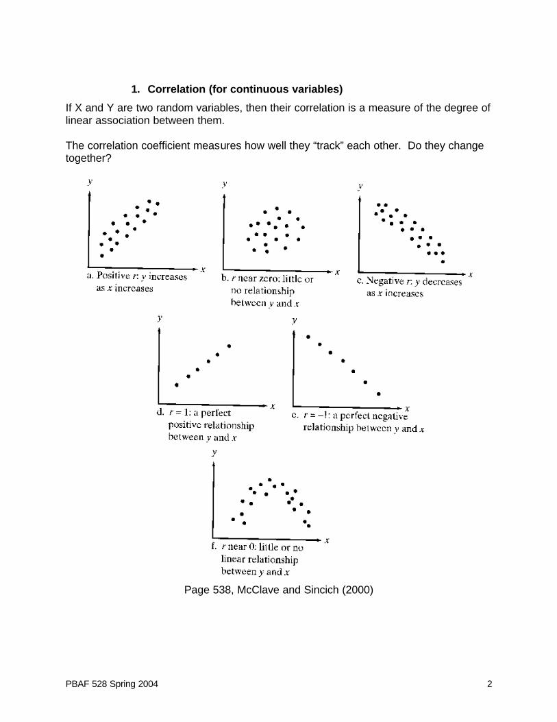
1. Correlation (for continuous variables)
If X and Y are two random variables, then their correlation is a measure of the degree of linear association between them. The correlation coefficient measures how well they “track” each other. Do they change together?
Page 538, McClave and Sincich (2000)

PBAF 528 Spring 2004 3
ρ population correlation coefficient; it equals between –1 and +1 (say rho)
r sample correlation coefficient; it equals between –1 and +1
The closer the correlation coefficient is to –1 or +1, the stronger the linear relationship (negative or positive respectively). We can say they are strongly correlated.
The closer it is to 0, the weaker the linear relationship.
Let’s look at some examples:
Correlations with Household Income HH income Poverty Level .770 Hours worked per week .069 # of phone lines .139 # of people living in house .041 Age -.020 Wages per week .357
To calculate a sample correlation coefficient use SPSS or Excel (see Assignment 1) or:
( )( )
( ) ( )
−
−
−==
∑∑∑∑
∑ ∑∑
ny
ynx
x
nyx
xyr
2
2
2
2yyxx
xy
SSSS
SS
Often we want to know if the population value of the correlation, ρ, is different from 0 based on what we observe the correlation to be in our sample, r?
Null hypothesis: ρ=0 Alternative hypothesis: ρ≠0
Test statistic:
21 2
−−
=
nr
rt
for t with n-2 df
Could be one-tailed (is the correlation positive only? negative only?) Could be two-tailed (is this correlation different from zero?)
Decision rule: Select a significance level (α). If t>tα we can reject the null hypothesis.

PBAF 528 Spring 2004 4
C. Causation
Does A cause B? eg: Does distance to work cause travel time? Does one cause the other? Can we find out all the unique causes? (idiographic) OR Only the most important (monothetic)--those that explain the most variation? Conditions for establishing causation:
⇒ The cause precedes the effect in time. ⇒ Empirically correlated with each other ⇒ The observed correlation cannot be explained in terms of some third variable that
causes both of them. Necessary cause
Sufficient cause THINK CRITICALLY ABOUT CAUSATION! What else could be causing the relationship?
D. Course Syllabus and Requirements
PBAF 528 Spring 2004 5
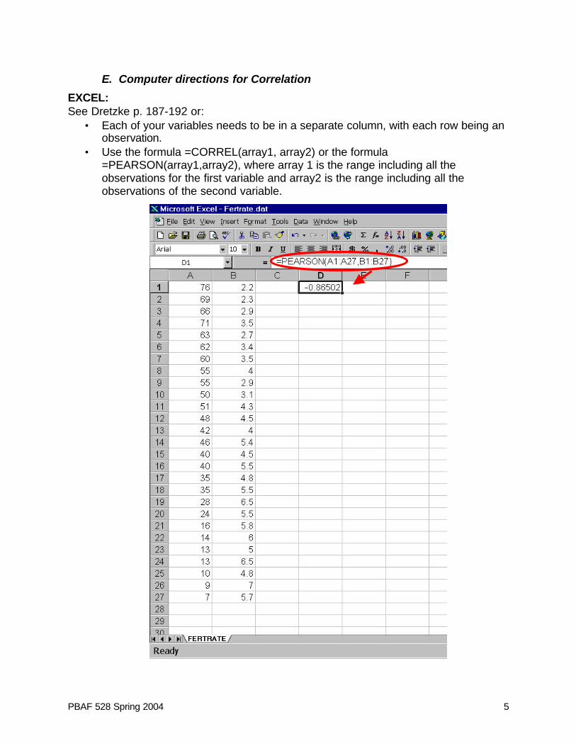
E. Computer directions for Correlation
EXCEL: See Dretzke p. 187-192 or:
• Each of your variables needs to be in a separate column, with each row being an observation.
• Use the formula =CORREL(array1, array2) or the formula =PEARSON(array1,array2), where array 1 is the range including all the observations for the first variable and array2 is the range including all the observations of the second variable.

PBAF 528 Spring 2004 6
SPSS: See Carver and Nash p. 52-54 or: • Select ANALYZE>CORRELATE>BIVARIATE • Select the first variable from the list. Click the arrow to move it to the “Variables”
box. • Select the second variable from the list. Click the arrow to move it to the
“Variables” box. • Make sure the box in front of “Pearson” is checked. • Make sure you have the tails box checked appropriately. • Click OK.
PBAF 528 Spring 2004 7
2. Regression Analysis and the Research Process
A. Simple Linear Regression—Bivariate Relationships Continued
We are looking for the line that minimizes the distance through all the points in the scatter plot.
⇒ The actual outcomes are spread around this "best guess" line. Algebra equation for a line: Y = MX + B In regression we write this as: Y = β1X + β0 + ε usually Y = β0 + β1X + ε (Regress Y on X) Y is the outcome variable—the dependent variable. X is the explanatory or predictor variable -- the independent variable. β0 is where the line hits the vertical axis -- the constant term. β1 is XY ∆∆ —the amount of change in Y for a unit change in X--the slope
ε is random unexplained noise, other explanatory factors, measurement error, or another equation with a different form—the residual or error.
NB: Y is not known exactly as soon as we know X, but our estimate of it is
narrowed down. We know the mean value of Y associated with that particular X, because of the relationship that we observe in the data.
“The best guess" line will depend on which cases were in the sample (we have the sampling distribution that provides SEs, p values, and hypothesis testing). There are two unknown population parameters β0 and β1 out there, but we will have to rely on a sample to estimate them. So, we estimate an equation and produce estimated regression coefficients (beta-hats):
ii e++= XˆˆY 10i ββ
The subscript letter i takes values from 1 to n (there are n data points). Each value ei is the distance from the fitted regression line estimate of y to the ith datapoint y.
iY is the value of Y lying on the fitted regression line for a given value of X.
1. Common mistake about regression and correlation
People often think that as the slope of the estimated regression line gets larger, so does r. But in fact r really measures how close all the data points are to our estimated regression line, not how steep the slope of the regression line is. If the points while exactly on the line, then the correlation is either +1 or -1, regardless of the slope, unless the slope is 0. If there is no linear relationship, then r = 0.
PBAF 528 Spring 2004 8
B. More simple linear regression
From a sample we estimate the following equation:
ii e++= XˆˆY 10i ββ
Ordinary Least Squares (OLS) gives estimates of model parameters. ⇒ Minimizes the sum of the square distances between the data points and the
fitted line. ⇒ Coefficients weight “outliers” more, since residuals are squared. ⇒ Precision of these estimates (SE) depends on sample size (larger is better),
amount of noise (less is good), amount of variation in explanatory factor (more is good).
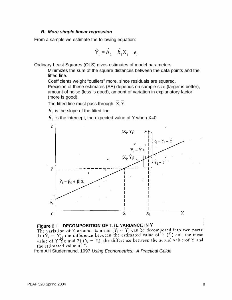
⇒ The fitted line must pass through Y,X
⇒ 1β is the slope of the fitted line
⇒ 0β is the intercept, the expected value of Y when X=0
from AH Studenmund. 1997 Using Econometrics: A Practical Guide

PBAF 528 Spring 2004 9
The straight-line regression model assumes four things: ⇒ X and Y are linearly related ⇒ The only randomness in Y comes from the error term, not from uncertainty
about X ⇒ The errors are normally distributed with mean 0 and variance σ2 ⇒ The errors associated with various datapoints are uncorrelated (not related to
each other) To estimate the coefficients for a regression line with just one dependent variable and one independent variable:
xy 10ˆˆ ββ −=
( ) ( )[ ]( ) ( )
∑ ∑∑ ∑∑
∑
∑
−
−=
−
−⋅−==
=
=
n
xx
n
yxyx
xx
yyxx
SS
SS
ii
iiii
n
ii
n
iii
xx
xy2
2
1
2
11β
PBAF 528 Spring 2004 10
C. An Aside about the Research Process--Points to Address in a Research Proposal
In the proposal, make sure you respond to each of these points.
1. Formulate a question/problem
2. Review the literature and develop a theoretical model
⇒ What else has been done on this? What theories address it?
3. Specify the model: independent and dependent variables
4. Hypothesize about the expected signs of the coefficients
⇒ Translate your question into specific hypotheses
5. Collect the data/operationalize
⇒ all variables have same number of observations ⇒ unit of analysis (person, month, year, household) ⇒ degrees of freedom (at least 1 more than the number of parameters—more is
better)
6. Analysis
⇒ In the case of regression, estimate and evaluate the equation ⇒ In the proposal, discuss what analyses will you undertake.
7. Document
⇒ In the proposal, explain how you will document all of the above ⇒ Discuss implications ⇒ Avoid ecological fallacy in interpretation
PBAF 528 Spring 2004 11
3. Interpreting results
A. Goodness of Fit
OLS solves for the estimates of β0 and β1 that minimizes the squares of the distances between data points and predicted values (residuals). SSyy = SSyy- SSE +SSE (your book)
( )∑=
−n
i 1
2
i yy = ( )∑=
−n
i
y1
2iy + ( )∑
=
−n
iii yy
1
2ˆ
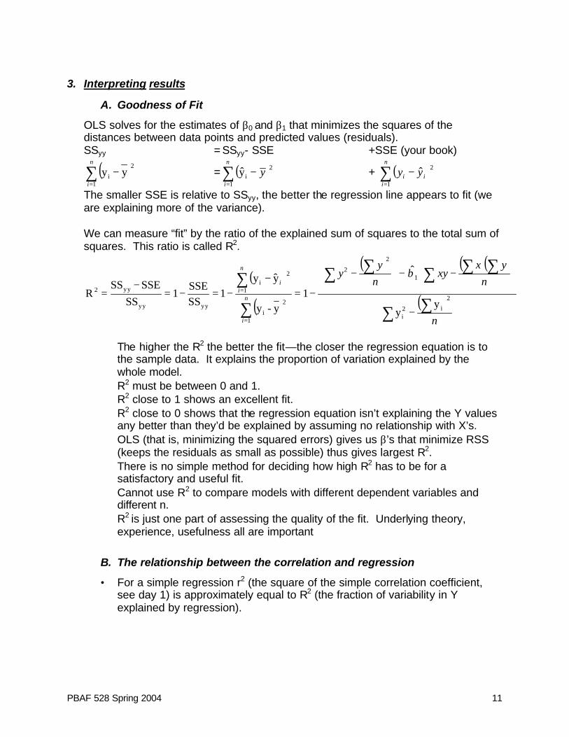
The smaller SSE is relative to SSyy, the better the regression line appears to fit (we are explaining more of the variance). We can measure “fit” by the ratio of the explained sum of squares to the total sum of squares. This ratio is called R2.
( )
( )
( ) ( )( )
( )∑ ∑
∑ ∑∑∑∑
∑
∑
−
−−
−
−=−
−=−=−
=
=
=
n
nyx
xyny
y
n
i
n
ii
2
i2i
1
2
2
1
2
i
1
2i
yyyy
yy2
yy
ˆ
1y-y
yy1
SSSSE
1SS
SSESSR
β
⇒ The higher the R2 the better the fit—the closer the regression equation is to
the sample data. It explains the proportion of variation explained by the whole model.
⇒ R2 must be between 0 and 1. ⇒ R2 close to 1 shows an excellent fit. ⇒ R2 close to 0 shows that the regression equation isn’t explaining the Y values
any better than they’d be explained by assuming no relationship with X’s. ⇒ OLS (that is, minimizing the squared errors) gives us β’s that minimize RSS
(keeps the residuals as small as possible) thus gives largest R2. ⇒ There is no simple method for deciding how high R2 has to be for a
satisfactory and useful fit. ⇒ Cannot use R2 to compare models with different dependent variables and
different n. ⇒ R2 is just one part of assessing the quality of the fit. Underlying theory,
experience, usefulness all are important
B. The relationship between the correlation and regression
• For a simple regression r2 (the square of the simple correlation coefficient, see day 1) is approximately equal to R2 (the fraction of variability in Y explained by regression).
PBAF 528 Spring 2004 12
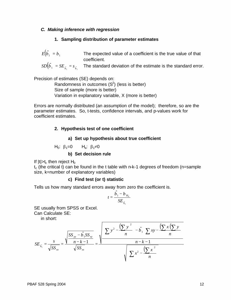
C. Making inference with regression
1. Sampling distribution of parameter estimates
( ) 11
ˆ ββ =E The expected value of a coefficient is the true value of that coefficient.
( )11
ˆˆ1ˆ
βββ sSESD == The standard deviation of the estimate is the standard error.
Precision of estimates (SE) depends on:
⇒ Randomness in outcomes (S2) (less is better) ⇒ Size of sample (more is better) ⇒ Variation in explanatory variable, X (more is better)
Errors are normally distributed (an assumption of the model); therefore, so are the parameter estimates. So, t-tests, confidence intervals, and p-values work for coefficient estimates.
2. Hypothesis test of one coefficient
a) Set up hypothesis about true coefficient
H0: β1=0 Ha: β1≠0
b) Set decision rule
If |t|>tc then reject H0 tc (the critical t) can be found in the t table with n-k-1 degrees of freedom (n=sample size, k=number of explanatory variables)
c) Find test (or t) statistic
Tells us how many standard errors away from zero the coefficient is.
1
0
ˆ
1ˆ
β
ββ
SEt H−
=
SE usually from SPSS or Excel. Can Calculate SE:
in short:
( ) ( )( )
( )
−
−−
−−
−
=−−−
==∑∑
∑ ∑∑∑∑
nx
x
kn
n
yxxy
n
yy
SSkn
SSSS
SSs
SExx
xyyy
xx2
2
1
2
2
1
ˆ1
ˆ
1
ˆ
1
ββ
β

PBAF 528 Spring 2004 13
d) Compare critical t and test statistic
3. Problems with hypothesis tests
a) Type I Error
Reject the null when the null is true. The p-value tells us the chance of making this type of error
b) Type II Error
We fail to reject the null when the null is false. The chances of making this type of error decreases with larger sample sizes, with larger standard errors of the parameter estimate, and with the size of the true parameter.
D. Confidence Interval for parameter estimate
A (1-α)% confidence interval for the true coefficient (the slope or β on some predictor X) is given by:
1ˆ,211
ˆβαβ SEt df−± , where we use t at n-k-1 degrees of freedom.
E. P-value
Probability that you would get an estimate so far (in SEs) from βH0 if H0 were true. • p-values give the level of support for H0 • you can look up t-statistic in t or z table (or use Excel) to find the probability in the
tail.

PBAF 528 Spring 2004 14
4. What About Other Causal Factors?
A. Framing a Research Question
What if we were interested in the impact of rent control on homelessness? What is our question? How does our question shape how we approach finding the answer? Why might rent control cause homelessness? How about another question: How do we know if a vaccine is effective?
B. Experiments and Quasi-Experiments
Does the presence of the independent variable cause some change in the dependent (outcome) variable? How do we rule out all the other potential causes and attribute a change only to our factor of interest?
One Shot Case Study In depth study, can’t be sure of effects of independent variable, though.
Pretest-posttest That is, before and after some stimulus; but still don’t know what changes would have been over time without stimulus.
Experiment and Control group Two randomly assigned groups. One gets the treatment, the other doesn't. Sometimes the experiment itself causes an effect, the Hawthorne effect.
Internal Validity: Does the stimulus really cause the change in the dependent
variable? . External Validity: Generalizability

PBAF 528 Spring 2004 15
C. Multiple Regression
Much of the time, we don’t have the money to do an experiment with random assignment. Or it is unethical. Or it is impractical. We still have to deal with the issue of multiple causes. For example, there is likely some relationship between education and income, but we cannot randomly assign people to more or less education, or rule out all the threats to internal validity, we can try to do this through multiple regression.
Multivariate regression model
εββββ ++++= nn X...XXY 22110
⇒ β0 is the intercept--the expected value of Y if all explanatory factors are zero ⇒ β1 is the effect of a one unit change in X1 on Y, holding constant all other
explanatory variables (X2)
⇒ β2 is the effect of a one unit change in X2 on Y, holding constant X1
⇒ In this linear model, the effect on the outcome of a change in an explanatory variable (the slope) is the same regardless of where you start.
For a sample: enn ++++= Xˆ...XˆXˆˆY 22110 ββββ
1. More on Goodness of Fit—Multiple Xs
With multiple Xs, OLS solves for the estimates of β0, β1, and β2 that minimizes the squares of the distances between data points and predicted values (residuals). SSyy = SSyy- SSE +SSE (your book) TSS = ESS + RSS Total Sum of Squares = Explained Sum of Squares + Residual Sum of Squares
( )∑=
−n
i 1
2
i YY = ( )∑=
−n
i 1
2
i YY + ∑=
n
iie
1
2[this = ( )∑
=
−n
iii YY
1
2ˆ ]
With multiple Xs, it is still true that the smaller SSE is relative to SSyy, the better the regression line appears to fit (we are explaining more of the variance). R2 is still the measure of fit, calculated as the ratio of the explained sum of squares to the total sum of squares:
( )( ) ( )∑
∑
∑
∑
=
=
=
= −=−
−=−=−
== n
i
n
ii
n
i
n
iii eYY
1
2
i
1
2
1
2
i
1
2
yyyy
yy2
Y-Y1
Y-Y
ˆ
1SSSSE1
SS
SSESS
TSSESSR

PBAF 528 Spring 2004 16
⇒ The higher the R2 the better the fit—the closer the regression equation is to the sample data. It explains the proportion of variation explained by the whole model.
⇒ R2 must be between 0 and 1. ⇒ R2 close to 1 shows an excellent fit. ⇒ R2 close to 0 shows that the regression equation isn’t explaining the Y values
any better than they’d be explained by assuming no relationship with X’s. ⇒ OLS (that is, minimizing the squared errors) gives us β’s that minimize RSS
(keeps the residuals as small as possible) thus gives largest R2. ⇒ There is no simple method for deciding how high R2 has to be for a
satisfactory and useful fit. ⇒ Cannot use R2 to compare models with different dependent variables and
different n. ⇒ R2 is just one part of assessing the quality of the fit. Underlying theory,
experience, usefulness all are important Characteristics of R2 in multiple regression: When you add another variables, R2 always increases. So, we adjust R2 for the number of degrees of freedom--
2R (the adjusted R-squared—your book calls it
2aR )
The number of degrees of freedom is the number of data points above and beyond the number of coefficients that are being predicted. n-(k+1) or n-k-1, where n is the number of data points, k is the number of predictors, and adding 1 to k to account for the intercept.
( )
−−−−=
−
−
+−
−==
∑
∑
=
=
1)1(
1
))1((1RR 222
1
1
2
22a kn
kRR
n
YY
kn
e
n
i
n
ii
D. The relationship between the correlation and multiple regression
• While for a regression with one X and one Y r2 (the square of the simple correlation coefficient, see day 1) is approximately equal to R2 (the fraction of variability in Y explained by regression), this is not the case for multiple regression.
• Some x’s may be correlated with each other (this phenomenon is called multicollinearity) and you would expect them to the correlated to some extent or else you wouldn't need regression analysis to tease apart the relationships. If two X’s are highly correlated, then you don't need both of them to predict the Y value -- they are redundant that case.

PBAF 528 Spring 2004 17
E. Choosing Factors to Include: The role of theory
Source: Babbie (1st Edition) p. 39
F. What factors cause homelessness?
How much confidence can we have in our estimates?

PBAF 528 Spring 2004 18
G. In-Class Exercise
Does Rent Control Cause Homelessness?1 • Data from 50 U.S. Cities • Outcome is log of rate of homelessness • Rent control is “dummy variable” (0=no law, 1=rent control law) • Tucker’s coefficient on Rent Control is .42 t=3.99, n=50, k=3, tα=2.02 (at df n-k-1)
1 Quigley, John M. 1990. Journal of Policy Analysis and Management, pp. 89-93.
PBAF 528 Spring 2004 19
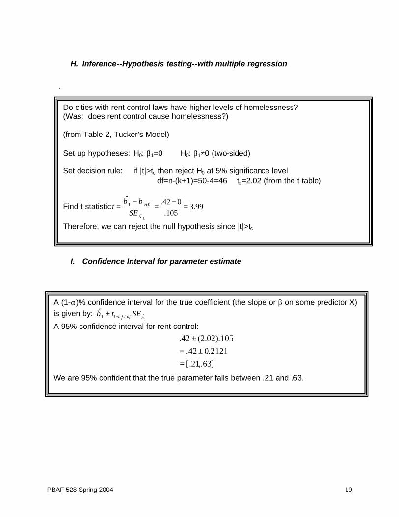
H. Inference--Hypothesis testing--with multiple regression
.
I. Confidence Interval for parameter estimate
Do cities with rent control laws have higher levels of homelessness? (Was: does rent control cause homelessness?) (from Table 2, Tucker’s Model) Set up hypotheses: H0: β1=0 H0: β1≠0 (two-sided) Set decision rule: if |t|>tc then reject H0 at 5% significance level df=n-(k+1)=50-4=46⇒ tc=2.02 (from the t table)
Find t statistic 99.3105.
042.ˆ
1ˆ
01 =−=−
=β
ββSE
t H
Therefore, we can reject the null hypothesis since |t|>tc
A (1-α)% confidence interval for the true coefficient (the slope or β on some predictor X) is given by:
1ˆ,211
ˆβαβ SEt df−±
A 95% confidence interval for rent control:
]63,.21[.
2121.042.105).02.2(42.
=±=
±
We are 95% confident that the true parameter falls between .21 and .63.

PBAF 528 Spring 2004 20
J. P-value
.
K. Discussion Questions
1. What do the adjusted R-squares for the models in Table 2 tell you? 2. How did the coefficient for rent control change from Tucker’s Model to Model I? How
about the change from Model I to Model II? What does the change suggest to you about rent control’s relationship with homelessness?
3. What does the change in the t-statistic for rent control for Tucker’s Model to Models I and II tell you?
4. How does Model III differ from the other two models? In your opinion, given what you have learned about hypothesis testing and goodness of fit, does this model explain homelessness better than the other models?
How likely is it that we’d get a coefficient of .42 if there were no relationship between homelessness and rent control? P[t>|3.99| if β1=0] <.01 (for df=46, 2-sided from table) Therefore, we would expect a t-statistic this big (an estimate this far from our hypothesized one) less than 1 percent of the time, if the null hypothesis were true. This does not mean that there is a one percent chance that the null hypothessis is true.

PBAF 528 Spring 2004 21
L. About omitted variables
1. Included coefficient is too high (toward positive) if
• the omitted factor is positively correlated with the outcome and included factor
or • the omitted factor is negatively correlated with the outcome and
included factor
2. Included coefficient is too low (toward negative) if
• the omitted factor is positively correlated with the outcome and negatively correlated with the included factor
or • the omitted factor is negatively correlated with the outcome and
positively correlated with the included factor
M. Classical Assumptions
About OLS and its estimators 1. The regression model is linear in the coefficients, is correctly specified, and has
an additive error term. 2. The error term has zero population mean. 3. All explanatory variables are uncorrelated with the error term. 4. Observations of the error term are uncorrelated with each other (no serial
correlation). 5. The error term has a constant variance (no heteroskedasticity). 6. No explanatory variable is a perfect linear function of any other explanatory
variable. 7. The error term is normally distributed.
Given these seven classical assumptions the OLS coefficient estimators can be shown to have the following properties:
⇒ Unbiased ⇒ Minimum Variance ⇒ Consistent ⇒ Normally distributed
OR, OLS is BLUE (Best Linear Unbiased Estimator)

PBAF 528 Spring 2004 22
N. Reporting requirements
1. Required elements
⇒ Data source or sources (time, duration, place, units, method of data collection)
⇒ Sample size (n) ⇒ Descriptive statistics for dependent and independent variables (mean, SD) ⇒ Coefficients for the regression model ⇒ Standard errors for coefficients (and/or t statistics—next time!)
⇒ Goodness of fit (R2, 2
R , or others like log-likelihood (for discrete outcomes—we’ll get to this)
⇒ Issues of concern or debate
2. Possible Additions
⇒ Predicted values for important cases ⇒ Confidence intervals around coefficients (next time!) ⇒ Standardized coefficients or elasticities ⇒ Alternative regression models ⇒ Regressions on selected subsets of your sample

PBAF 528 Spring 2004 23
5. Interpreting Results--Reprise
A. Comments about hypotheses and hypothesis testing
1. A hypothesis states the relationship between two variables.
A hypothesis needs to clearly state a prediction about a relationship and the unit of analysis for this relationship.
2. Hypothesis testing is about statistical significance, not theoretical validity.
There are variables whose relationship is statistically significant but have no theoretical basis for being related. Likewise, there are theoretical relationships that may not turn out to be statistically significant (due to sample size or limited to variability in X in the data set) but should be included in your model for completeness. All of this takes judgment.
3. T-tests do not test importance of the coefficient.
The magnitude of the coefficient (that is, the slope 1β , 2β , etc) is a separate issue from the magnitude of the t-statistic (which tells you how confident to be about the coefficient estimate).
4. T-tests are intended for use on samples.
Use a t-test with relatively small samples, not with data for the entire population. With very large samples you can reject almost any null hypothesis.
1
1ˆ
β
βSE
t = and as sample size increases, SE diminishes and t approaches infinity, but
this doesn't mean that the true β is not really zero, just that it is a large number of SEs away from zero (but as SEs become very small of this starts to be less important).
PBAF 528 Spring 2004 24
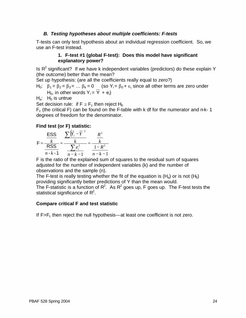
B. Testing hypotheses about multiple coefficients: F-tests
T-tests can only test hypothesis about an individual regression coefficient. So, we use an F-test instead.
1. F-test #1 (global F-test): Does this model have significant explanatory power?
Is R2 significant? If we have k independent variables (predictors) do these explain Y (the outcome) better than the mean? Set up hypothesis: (are all the coefficients really equal to zero?) H0: β1 = β2 = β3 = … βk = 0 (so Yi = β0 + εi, since all other terms are zero under
H0, in other words Y i = Y + ei) Ha: H0 is untrue Set decision rule: if F ≥ Fc then reject H0 Fc (the critical F) can be found on the F-table with k df for the numerator and n-k- 1 degrees of freedom for the denominator. Find test (or F) statistic:
( )
11
1
ˆ
2
2
2
2
−−−
=
−−
−
==∑
∑
knR
kR
kne
k
YY
kn
ki
i
1--RSS
ESS
F
F is the ratio of the explained sum of squares to the residual sum of squares adjusted for the number of independent variables (k) and the number of observations and the sample (n). The F-test is really testing whether the fit of the equation is (Ha) or is not (H0) providing significantly better predictions of Y than the mean would. The F-statistic is a function of R2. As R2 goes up, F goes up. The F-test tests the statistical significance of R2. Compare critical F and test statistic If F>Fc then reject the null hypothesis—at least one coefficient is not zero.

PBAF 528 Spring 2004 25
2. F-test #2: Do a subset of predictors add to the explanatory power of the model?
Would a model with fewer explanatory variables be just as good? First, we create an equation with a set of constraints or restrictions that are put on the regression equation. So, the regression equation is written as if the null hypothesis were true. For this test, that a subset of coefficients are equal to zero. Second, we compare the fit of this constrained equation to an equation that is unconstrained (or unrestricted) -- where the subset of coefficients are allowed to vary from zero. One equation must be a subset of the other in order to compare them. Hypothesis: (are a subset of coefficients really equal to zero?)
Restricted equation (null model)
εββ ++= 110 XY
H0: βi…=βM=0 (all M coefficients are zero)
Unrestricted equation εβββ ++++= MM XXY ...110
Ha: All M coefficients are not zero.
Find test (F) statistic: Can be expressed in terms of RSS or R2:
1--RSS
MRSSRSS
FUR
URR
1)-k-n(M,
kn
−
=
11
−−−
−
=
kn
2UR
2R
2UR
1)-k-n(M, RM
RR
F
M is the number of constraints on the equation. M of the k variables are omitted (set equal to 0 under the H0). RSSR is the residual sum of squares (unexplained sum of squares) under the restricted or constrained equation and RSSR≥RSSUR
You need to calculate the RSSR and the RSSUR. So, you first run the regression with all the independent variables included and get RSSUR (this is the original regression model). Then run the regression without the M variables (this assumes that they have all been set to zero and gives a new regression model) and get the RSSR. The two equations must have the same number of cases. Decision rule: if F(M,n-k-1) ≥ Fc then reject H0
Rejecting the null means that not all of the coefficients are zero. Example: As a group, do gender and race provide information about differences in earnings?
PBAF 528 Spring 2004 26
C. Computer Directions for F-tests
1. F-test #1: Does this model have significant explanatory power?
To test the explanatory power of the whole set of explanatory variables, as compared to just using the overall mean of the outcome variable, use the F-statistic and the p-value printed by SPSS or Excel under “ANOVA.” If this p-value is less than 0.05, you can reject the null hypothesis (which is that all of the variables have coefficients of zero) at the 5% significance level. If the p-value is less than 0.01 you can reject at the 1% significance level.
2. F-test #2: Do a subset of predictors add to the explanatory power of the model?
To test if, as a group, a subset of explanatory variables have significant explanatory power, you must first run one regression that includes all explanatory variables and then a second regression with only the subset you want to test. In Excel, you’ll just have to run the regressions twice, once with all the regressors and once with only a subset. The use the R2 from each model to compare them as outlined in the lecture notes. In SPSS there is a shortcut. Click on ANALYSIS, REGRESSION, LINEAR and designate your DEPENDENT VARIABLE. Put in all the variables (both those you are testing and those you are not testing) as INDEPENDENT VARIABLES. Now, you'll see BLOCK 1 of 1; click on NEXT to move to the next "block" of explanatory variables. Put in the list of independent variables that you want to test (your subset of variables). Click on METHOD and change this to REMOVE. This will cause SPSS to run to regression equations when you click run. The first will include all of your variables and the second run a regression without the variables you specified. Use the R2 or residual sum of squares under "ANOVA" to do the F-test as illustrated in the lecture notes.

PBAF 528 Spring 2004 27
D. Using Models for Prediction
You used a regression model for prediction in assignment 1, when you found out the predicted time to campus for someone who lived at the average distance away. You can use an estimated regression model to predict the dependent variable for different values of the independent variables. For example, what if we wanted to predict the level of homelessness in average cities with and without rent control? And suppose we thought Tucker’s model was a good one. Based on his estimates, we know the following:
( ) ( ) ( )GrowthPercent 005.0eTemperatur017.0ControlRent 42.0484.0ssHomelessne −++−=∧
We can substitute the means for temperature and percent growth. A city with rent control has a 1 in that spot, a 0 without. So, let’s compare: With rent control:
( ) ( ) ( )1.49-005.056.94017.0142.0484.0ssHomelessne −++−=∧
91.00745.0968.042.0484.0
=−++−=
Remember, homelessness was logged, so take the inverse to be able to interpret (you don’t need to this if the DV isn’t logged!):
484.291. =e homeless per thousand Without rent control:
( ) ( ) ( )1.49-005.056.94017.0042.0484.0ssHomelessne −++−=∧
49.00745.0968.00484.0
=−++−=
Again, remember homelessness was logged, so take the inverse to be able to interpret (you don’t need to this if the DV isn’t logged!):
631.149. =e homeless per thousand
We see that not only did the coefficient show there to be a difference, but we can predict the expected value (the average) associated with the difference.

PBAF 528 Spring 2004 28
E. In-Class Exercise: Hypothesis testing and prediction
An local community development corporation (CDC) is trying to value 2 multifamily properties it redeveloped when it first started as a CDC, 15 years ago. As their summer intern, your boss at the CDC asks you to look into this. You boss took a sample of 25 multifamily buildings at random from all buildings sold during a recent year as a way to begin the analysis and then ran some regression models. Use the list of questions that follow to help guide your analysis. The data, summary statistics, and models are on the following pages. Your boss used Excel because that’s what she had on her computer.
1. Do each of the models presented have significant explanatory power? How do you
know? 2. Does the number of parking areas in combination with the age of the structure and
lot size add to the explanatory power of the model? (Compare model 1 with model 2) (HINT: remember that on Excel printout, the ESS and RSS are in the ANOVA table. The ESS (explained sum of squares) is called “regression” and RSS (residual sum of squares) is called residual.)
3. Given the print out you’ve seen so far and the tests that you’ve conducted, what variables do you think should remain in the model? Is there other information you’d like before you settle on a model?
4. Based on Model 2, tell your boss the predicted sale values for the two buildings. Here are the characteristics:
Characteristic Building 1 Building 2 No. of Apartments 14 30 Age of Structure 85 15 Lot Size 11,745 21000 No. of On-Site Parking Spaces 0 30 Gross Building Area 23,704 30,000

PBAF 528 Spring 2004 29
Table 1: Random Selection of Multifamily Buildings Code No Sale
Price ($) No of
Apartments Age of
Structure Lot size No of On-site
parking spaces
Gross Building
Area 229 90300 4 82 4365 0 4266 94 384000 20 13 17798 0 14391 43 157500 5 66 5913 0 6615 79 676200 26 64 7750 6 34144
134 165000 5 55 5150 0 6120 179 300000 10 65 12506 0 14552 87 108750 4 82 7160 0 3040
120 276538 11 23 5120 0 7881 246 420000 20 18 11745 20 12600 25 950000 62 71 21000 3 39448 15 560000 26 74 11221 0 30000
131 268000 13 56 7818 13 8088 172 290000 9 76 4900 0 11315 95 173200 6 21 5424 6 4461
121 323650 11 24 11834 8 9000 77 162500 5 19 5246 5 3828 60 353500 20 62 11223 2 13680
174 134400 4 70 5834 0 4680 84 187000 8 19 9075 0 7392 31 155700 4 57 5280 0 6030 19 93600 4 82 6864 0 3840 74 110000 4 50 4510 0 3092 57 573200 14 10 11192 0 23704
104 79300 4 82 7425 0 3876 24 272000 5 82 7500 0 9542
Table 2: Descriptive Statistics
Data Total Average of Sale Price ($) 290,573.52 StdDev of Sale Price ($) 211,529.15 Average of No of Apartments 12.16 StdDev of No of Apartments 12.58 Average of Age of Structure 52.92 StdDev of Age of Structure 25.89 Average of Lot size 8,554.12 StdDev of Lot size 4,199.30 Average of No of On-site parking spaces 2.52 StdDev of No of On-site parking spaces 4.93 Average of Gross Building Area 11,423.40 StdDev of Gross Building Area 10,019.35
PBAF 528 Spring 2004 30
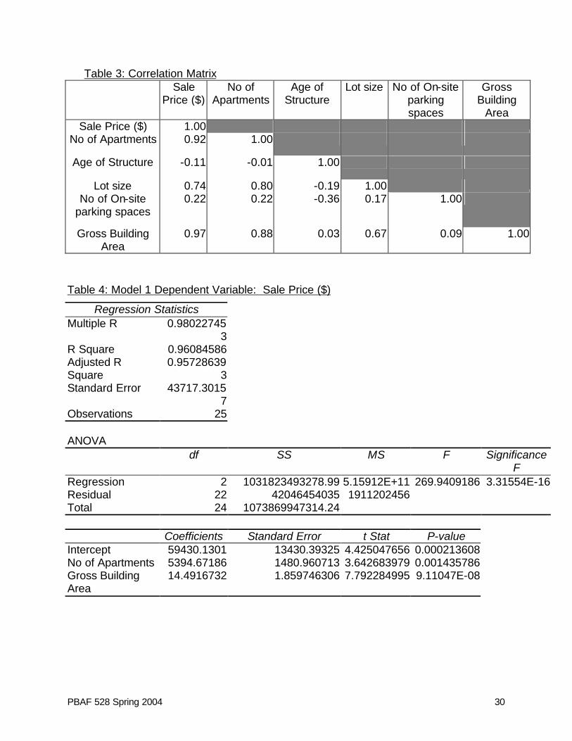
Table 3: Correlation Matrix Sale Price ($)
No of Apartments
Age of Structure
Lot size No of On-site parking spaces
Gross Building
Area Sale Price ($) 1.00
No of Apartments 0.92 1.00
Age of Structure -0.11 -0.01 1.00
Lot size 0.74 0.80 -0.19 1.00 No of On-site
parking spaces 0.22 0.22 -0.36 0.17 1.00
Gross Building Area
0.97 0.88 0.03 0.67 0.09 1.00
Table 4: Model 1 Dependent Variable: Sale Price ($)
Regression Statistics Multiple R 0.98022745
3
R Square 0.96084586 Adjusted R Square
0.957286393
Standard Error 43717.30157
Observations 25
ANOVA df SS MS F Significance
F Regression 2 1031823493278.99 5.15912E+11 269.9409186 3.31554E-16 Residual 22 42046454035 1911202456 Total 24 1073869947314.24
Coefficients Standard Error t Stat P-value
Intercept 59430.1301 13430.39325 4.425047656 0.000213608 No of Apartments 5394.67186 1480.960713 3.642683979 0.001435786 Gross Building Area
14.4916732 1.859746306 7.792284995 9.11047E-08
PBAF 528 Spring 2004 31
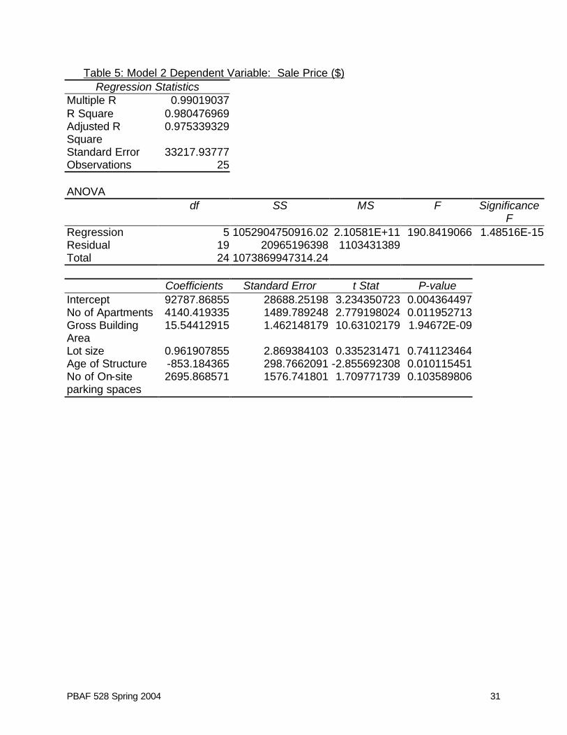
Table 5: Model 2 Dependent Variable: Sale Price ($) Regression Statistics
Multiple R 0.99019037 R Square 0.980476969 Adjusted R Square
0.975339329
Standard Error 33217.93777 Observations 25
ANOVA
df SS MS F Significance F
Regression 5 1052904750916.02 2.10581E+11 190.8419066 1.48516E-15 Residual 19 20965196398 1103431389 Total 24 1073869947314.24
Coefficients Standard Error t Stat P-value
Intercept 92787.86855 28688.25198 3.234350723 0.004364497 No of Apartments 4140.419335 1489.789248 2.779198024 0.011952713 Gross Building Area
15.54412915 1.462148179 10.63102179 1.94672E-09
Lot size 0.961907855 2.869384103 0.335231471 0.741123464 Age of Structure -853.184365 298.7662091 -2.855692308 0.010115451 No of On-site parking spaces
2695.868571 1576.741801 1.709771739 0.103589806
PBAF 528 Spring 2004 32
6. The Hunt for Data and Quiz Preview
A. Where can we find data?
• The Web • CSSCR • Publications • Personal contacts (privacy issues?)
B. In what form is data when we get it?
• Text file (ASCII): delimited or not? • SPSS, SAS
C. How do we need to manipulate data when we get it?
• Continuous or Discrete? • Transformations • Cleaning • Missing cases, missing variables
D. Quiz preview
1. Conditions for causation
2. Correlation
3. Simple and multiple linear regression
• The relationship between correlation and regression • Coefficient interpretation • Measures of Goodness of Fit: R-Square, Adjusted R-Square • Hypothesis testing for one coefficient (t-tests, p-values) • Confidence intervals for estimated coefficient values • What tests would you use to test hypothesis for multiple coefficients? (why
use F-tests #1 and #2) • Why is the estimated regression coefficient a good estimate of the true
regression coefficient? • Prediction with regression equations.
7. Quiz I
PBAF 528 Spring 2004 33
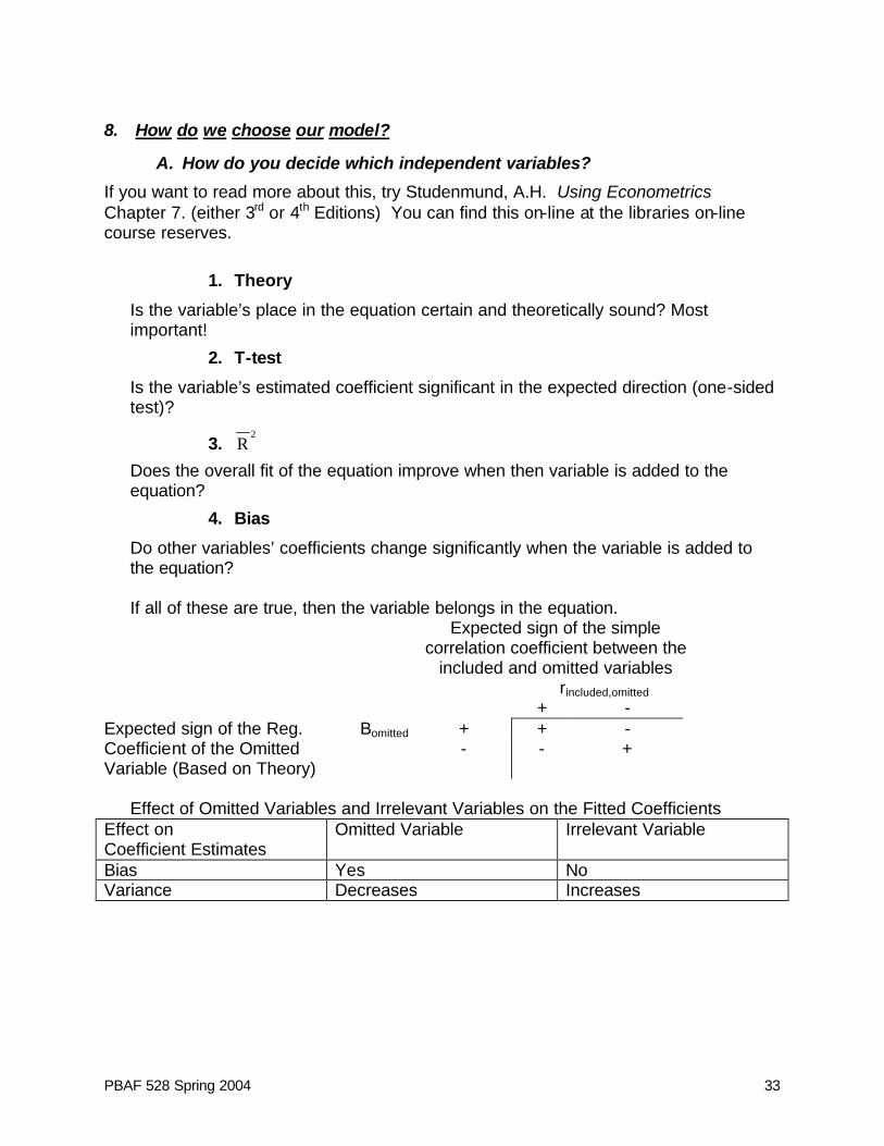
8. How do we choose our model?
A. How do you decide which independent variables?
If you want to read more about this, try Studenmund, A.H. Using Econometrics Chapter 7. (either 3rd or 4th Editions) You can find this on-line at the libraries on-line course reserves.
1. Theory
Is the variable’s place in the equation certain and theoretically sound? Most important!
2. T-test
Is the variable’s estimated coefficient significant in the expected direction (one-sided test)?
3. 2
R
Does the overall fit of the equation improve when then variable is added to the equation?
4. Bias
Do other variables’ coefficients change significantly when the variable is added to the equation? If all of these are true, then the variable belongs in the equation.
Expected sign of the simple correlation coefficient between the
included and omitted variables rincluded,omitted
+ - Expected sign of the Reg. Bomitted + + - Coefficient of the Omitted Variable (Based on Theory)
- - +
Effect of Omitted Variables and Irrelevant Variables on the Fitted Coefficients
Effect on Coefficient Estimates
Omitted Variable Irrelevant Variable
Bias Yes No Variance Decreases Increases

PBAF 528 Spring 2004 34
B. Dummy variables
Also called indicator or categorical variables.
1. What are they?
0,1 to distinguish between 2 categories (eg: male or female; college degree or not; King county or the rest of the state; Africa or not) Can also use for more than two categories. You need one dummy to represent each category, EXCEPT one category gets designated as the reference category (or the omitted group). This category has no dummy (eg: one for each racial group except one; one for each education level but one). More on this later.
2. Intercept Dummy Variables
When you fit a regression model, the coefficients on the dummy variables indicate the difference in the intercept of the fitted line between the reference group and the targeted group. What does this mean?
⇒ The intercept of the fitted line for the reference group is β0, consistent with our nomenclature thus far.
⇒ The intercept of the fitted line for the selected or targeted group is β0+βdummy What does the regression equation look like with a dummy in it?
Yi = β0 + β1X + β2Di + εI
⇒ Remember, the dummy, Di takes only 0 or 1 ⇒ So, for the reference group, Di = 0 and the regression equation is
Yi = β0 + β1X + εi What’s the intercept for the reference group?
⇒ For the “indicated” group, Di=1 and the regression equation is Yi = β0 + β1X + β2+ εI
What’s the intercept for the indicated group? What does a graph of the regression line (for simple regression look like with a dummy in it?

PBAF 528 Spring 2004 35
from AH Studenmund. 1997 Using Econometrics: A Practical Guide p. 233
Example: Dummy Variable for 2 Categories (One Dummy Variable) Question: What is the difference in rent for people in King County versus the rest of the state? Using the WAPOP data, I’ve developed a model that says that rent (Q3P5) is a function of personal earnings, number of minutes getting to school of work, King County residence (vs. everywhere else), and the respondent’s age. MODEL 1: Q3P5 = β0 + β1(PEARN97) + β3(Q8P4) + β4(KING) + β2(AGE) +ε Q3P5 is Rent Q8p4 is number of minutes getting to work or school last week. To answer our research question, we need to understand what coefficient on King County tells us. (see next page for model results)

PBAF 528 Spring 2004 36
MODEL 1: Q3P5 = β0 + β1(PEARN97) + β3(Q8P4) + β4(KING) + β2(AGE) +ε Model Summary
Model R R Square Adjusted R Square
Std. Error of the Estimate
1 .333a .111 .107 224.34
ANOVA
Sum of Squares df Mean Square F Sig. Regression 6490340.558 4 1622585.140 32.241 .000
Residual 52188868.264 1037 50326.777 Total 58679208.822 1041
Coefficients
Unstandardized Coefficients
t Sig.
Model B Std. Error 1 (Constant) 468.757 23.925 19.593 .000 1997
PERSONAL EARNINGS (constructed)
.002217 .000 5.933 .000
King County Resident
137.051 16.379 8.367 .000
AGE OF PERSON (constructed)
-.572 .639 -.896 .370
# MINUTES GETTING TO SCHOOL/WORK LAST WK
.558 .331 1.685 .092
1. What does the equation for your regression line look like if you live in King County? 2. What does the equation for your regression line look like if you live outside King
County?

PBAF 528 Spring 2004 37
3. Draw a picture of the two lines in (1) and (2). Don’t worry about the exact slope. 4. What does the coefficient on the dummy mean? 5. How sure are we of the effect of living in King County?

PBAF 528 Spring 2004 38
CAUTION: Don’t include too many dummies or you’ll have to explain each data point! CAUTION: Don’t include a dummy that only takes a value of 1 for one data point! Some ideas for using dummy variables: • Could use dummy for seasonal changes if you have data where each case is at a
different time point. • Dummies can also be used to make a different slope on the relationship between X
and Y (called slope dummies) or can be used for dependent variables (we’ll get to this later).
Example: More than 2 categories (more than one dummy variable) Education can be thought of as (1) not having earned a high school diploma, (2) having earned a high school diploma, and (3) having more education than a high school diploma. Then we use two dummies. We’ll call them D1 and D2. D1=1 if you have a diploma and 0 otherwise, D2=1 if you have a BA and 0 otherwise. What are all the possibilities? you have more than a high school degree D1= _____ and D2= ____
you have a high school diploma and nothing beyond that
D1= ____ and D2= ____
you have not earned any diploma D1= ____ and D2= ____
PBAF 528 Spring 2004 39
C. Interaction Terms
⇒ Interaction terms are products of two or more independent variables (really). ⇒ Allow for differences in effect of an explanatory factor across categories or
levels of another factor ⇒ Can interact dummies or continuous variables. ⇒ For 2 dummies: coefficient on interaction gives the effect of having the
combination (over being in either category separately) ⇒ For a continuous and a dummy: coefficient on interaction gives the effect of
being in the category and the continuous effect (over the continuous effect or the category separately)
⇒ For two continuous variables: coefficient on the interaction givens the synergistic effect of the two variables in combination, rather than each one being held constant.
1. What does the regression equation look like with an interaction in it?
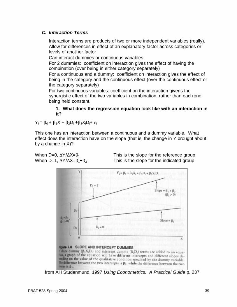
Yi = β0 + β1X + β2Di +β3XiDi+ εI
This one has an interaction between a continuous and a dummy variable. What effect does the interaction have on the slope (that is, the change in Y brought about by a change in X)? When D=0, ∆Y/∆X=β1 This is the slope for the reference group When D=1, ∆Y/∆X=β1+β3 This is the slope for the indicated group
from AH Studenmund. 1997 Using Econometrics: A Practical Guide p. 237

PBAF 528 Spring 2004 40
2. You need both the slope dummy and the intercept dummy in the equation.
The above regression line has both a slope dummy and an intercept dummy (a dummy that does not get multiplied by anything). This is necessary in most cases since just including a slope dummy would bias the slope by forcing it to explain more than it should, for example, changes in the mean between two groups. An intercept dummy best explains this sort of change. So, the model should include an intercept dummy (plain dummy term) where there is a slope dummy (a dummy multiplied by a predictor). Think carefully about your hypotheses about the direction of the relationship between the dummies and the outcomes since these terms make the model very flexible.
3. How do you test for significance of interaction terms?
⇒ To test for differences in slopes between the categories, use the t-test on the interaction term.
⇒ To test overall differences in the regression relationship with and without the inclusion of an interaction use an F-test (#2).

PBAF 528 Spring 2004 41
4. Example: Dummy Variable Interacting with a Continuous Variable
Does extensive media coverage of a military crisis influence public opinion on how to respond to the crisis? Political scientists at UCLA came up with a model concerning the 1990 Persian Gulf War, precipitated by Iraq leader Saddam Hussein’s invasion of Kuwait. They developed a model to analyze the level of support Americans had for military (rather than diplomatic) response to the crisis. The dependent variable ranges from 0 (preference for a diplomatic response) to 4 (preference for military response. Here is the model they developed based on data from 1,763 U.S. Citizens. E(y)=β0 + β1x1 + β2x2 +β3x3 +β4x4 +β5x5 +β6x6 +β7x7 +β8x2x3 +β9x2x4 where: x1 = Level of TV news exposure in a selected week (number of days) x2 = Knowledge of seven political figures (1 point for each correct answer) x3 = Dummy variable for Gender (1 if male, 0 if female) x4 = Dummy variable for Race (1 if nonwhite, 0 if white) x5 = Partisanship (0-6 scale, where 0 = strong Democrat and 6 = strong Republican) x6 = Defense spending attitude (1-7 scale, where 1 = greatly decrease spending and
7 = greatly increased spending) x7 = Education The regression results:
Variable β estimate Standard Error Two-Tailed p-Value TV news exposure (x1) .02 .01 .03 Political knowledge (x2) .07 .03 .03 Gender (x3) .67 .11 <.001 Race (x4) -.76 .13 <.001 Partisanship (x5) .07 .01 <.001 Defense spending (x6) .20 .02 <.001 Education (x7) .07 .02 <.001 Knowledge X Gender (x2x3) -.09 .04 .02 Knowledge X Race (x2x4) .10 .06 .08 R2=.194, F=46.88 (p<.001)
Source: Iyengar, S. and Simon, A. 1993. News coverage of the Gulf Crisis and public opinion. Communication Research 20,: 380 (Table 2)

PBAF 528 Spring 2004 42
1) Interpret the β estimates for TV news exposure. 2) Is there enough support to say that TV news exposure is associated with support
for a military resolution of the crisis? 3) Is there sufficient evidence to say that the relationship between support for a
military resolution and gender depends on political knowledge? 4) What is the effect of knowledge on support for military resolution for men? E(y)=β0 + β1x1 + β2x2 +β3(1) +β4x4 +β5x5 +β6x6 +β7x7 +β8x2(1) +β9x2x4 5) What is the effect of knowledge on support for military resolution for women? E(y)=β0 + β1x1 + β2x2 +β3(0) +β4x4 +β5x5 +β6x6 +β7x7 +β8x2(0) +β9x2x4 6) What test would you use to answer the following question: Overall, does gender
affect support for a military resolution?

PBAF 528 Spring 2004 43
5. Example: Interacting 2 continuous variables
Fowles and Loeb hypothesized that drunk driving fatalities are more likely at high altitude because higher elevations diminish the oxygen intake of the brain, which increases the impact of a given amount of alcohol.
ABADSBF iiiiii ⋅+−−+−−= 023.035.024.017.0024.033.2ˆ (t-statistics) (-0.8) (1.53) (-0.96) (-1.07) (1.97) Hypothesized relationship + + - + +? n=48, adjusted R2=.499 Fi= Traffic fatalities per vehicle mile (by state) Bi= per capita consumption of beer Si= average highway driving speed Di= dummy (1=state has a vehicle inspection program, 0=no inspection program) Ai= average altitude of metro areas (1000s of feet) The interaction in this model is between two continuous variables, consumption rate of beer and altitude. The effect on the outcome of each the two variables involved in the interaction depends on the interaction coefficient and the coefficient on the original variable. 1) Does the average altitude of metropolitan areas in the state affect the relationship between per capita beer consumption and the rate of traffic fatalities? 2) How much higher a fatality rate do we expect for an average altitude of metro area increase by 1000 feet? 3) Does the altitude affect the overall regression relationship explaining fatality rate? (How would you approach this?)

PBAF 528 Spring 2004 44
6. We could also have interactions between two dummy variables.
We could look at t-statistic for the interaction of the two dummies to see if the effect of being a member of both categories denoted by the dummies had an effect on the regression relationship. For example, look at the possible synergistic effect on earnings of being both black and female (all else held equal) you could run a regression in which you created one dummy to denote gender and another to denote race and then look at the t-statistic on the interaction of race and gender.

PBAF 528 Spring 2004 45
9. How do we choose our model? (continued)
We know that the β s are our estimate of the slope of the relationship between a predictor (explanatory factor), X, and an outcome, Y. The slope is the amount of change in the outcome that occurs when the predictor changes by “1 unit” (in units measured by the units of that variable). There are several other types of measures of the relationship between a predictor and an outcome.
A. Standardized regression coefficients
Show the expected change in outcome in standard deviations for a 1 standard deviation change in the explanatory factor. SPSS calculates this for us (but Excel will not). When you run a linear regression in SPSS they are in the table called “coefficients,” in the column called “Beta,” to the right of the standard error.
⇒ Best for continuous variables, not dummies or categoricals. ⇒ Can be used to compare the impact of variables just as β s can. ⇒ Allow you to compare the impacts of factors on the dependent variable
(they are on the same scale).
( )( ) 1
1ˆˆˆ edStandardiz 2
222
2222
−−∑
−−∑≡≡
nYY
nXXSD
SD
y
x βββ
So, if you are working in Excel and want to interpret standardized coefficients, you’ll have to create a formula to adjust each estimated coefficient.
How much (in standard deviations) would rent change with a 1 standard deviation change in personal earnings? From our model of factors predicting rent we find the standardized coefficient. We would expect rent to increase by .18 standard deviations for every 1 standard deviation change in personal earnings (PEARN97). We could also calculate this, using the descriptive statistics on rent (Q3P5) and personal earnings (PEARN97):
( )( ) 18.
42.23763.247,19
*002217.ˆˆ =≡≡Q3P5
PEARN97 edStandardiz PEARN97PEARN97 SD
SDββ

PBAF 528 Spring 2004 46
B. Elasticities
Show the expected percentage change in the outcome for a 1% change in the explanatory factor.
YX
XXYY 2
222
β=∆
∆≡≡
2xy,EElasticity
⇒ Must evaluated at a specific point, (X,Y), since elasticity is not constant
over the length of the regression line or plane. The specific point could be the mean of X and Y or any other X, Y point.
⇒ Can’t read these directly off SPSS or Excel output for a linear
regression since elasticity is not a constant.
What percentage would we expect rent to rise for a 1% increase in personal earnings? We’ll assess this at the mean of X and Y:
096.86.546
40.681,23002217.ˆ ==≡Y
X PEARN97PEARN97xy, PEARN97
E β
So, a 1% in personal earnings is associated with a .096% change in rent paid. What does a .096% change in rent paid mean?
52.0$86.546100096.0
=
So, rent goes up 52 cents for each additional $237 in annual personal earnings.
PBAF 528 Spring 2004 47
C. Does a straight line explain all relationships?
Not always! Sometimes theory or experience suggests that a linear functional form is inappropriate. So, you might consider a nonlinear form.
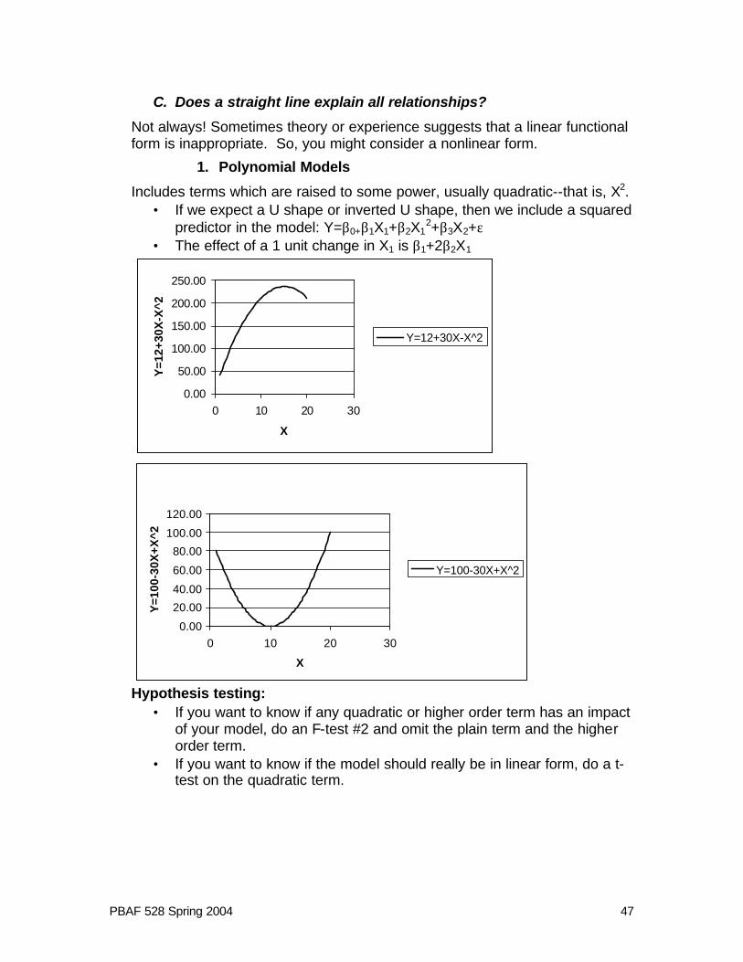
1. Polynomial Models
Includes terms which are raised to some power, usually quadratic--that is, X2. • If we expect a U shape or inverted U shape, then we include a squared
predictor in the model: Y=β0+β1X1+β2X12+β3X2+ε
• The effect of a 1 unit change in X1 is β1+2β2X1
0.00
50.00
100.00
150.00
200.00
250.00
0 10 20 30
X
Y=1
2+30
X-X
^2
Y=12+30X-X^2
0.00
20.00
40.00
60.00
80.00
100.00
120.00
0 10 20 30
X
Y=1
00-3
0X+X
^2
Y=100-30X+X^2
Hypothesis testing:
• If you want to know if any quadratic or higher order term has an impact of your model, do an F-test #2 and omit the plain term and the higher order term.
• If you want to know if the model should really be in linear form, do a t-test on the quadratic term.

PBAF 528 Spring 2004 48
2. Inverse Models
If the impact of a particular independent variable is expected to approach 0 as it increases, then you should use the inverse form in the regression model:
εβββ +++= 2210
1X
XY
1
• Effect of X on Y decreases quickly as X increases. • Can’t use for explanatory variables with 0 values. • A 1-unit change in X1 is associated with a -β1(1/Xi
2) change in Y.
Inverse
0
2
4
6
8
10
12
0 5 10 15 20 25
X
Y
Y=6+5*1/XY=6-5*1/X
An example is the relationship between rate of unemployment and the percentage change in wages. The theory is that the percentage change in wages is negatively related to the rate of unemployment, but past some level of unemployment, further increases in unemployment do not reduce the level of wage increases any further.

PBAF 528 Spring 2004 49
3. Logarithmic Models
Basically, logs are exponents. We typically use natural logs, which are logs in base e (e=2.718).
ln(x)=b means that eb=x so, since e2=7.389, ln(7.389)=2
Why do we use logs? • Logging depresses the number. • We use logs to reduce the absolute size of numbers and get at the
meaning behind them • We use logs to make it easy to figure out impacts in percentage terms.
We can log both explanatory and outcome variables but ONLY IF THEY ARE POSITIVE AND NON-ZERO. In SPSS or Excel, if you take the log of 0 or a negative number, you will get error messages. Often, when taking the log of income, economists will add 1 to the variable before taking the log (like in the homelessness/rent control example from class). When we log the dependent variable, the effect of a 1-unit change in X depends on the levels of all variables.
PBAF 528 Spring 2004 50
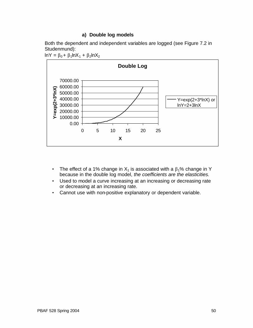
a) Double log models
Both the dependent and independent variables are logged (see Figure 7.2 in Studenmund): lnY = β0 + β1lnX1 + β2lnX2
Double Log
0.0010000.0020000.0030000.0040000.0050000.0060000.0070000.00
0 5 10 15 20 25
X
Y=e
xp(2
+3*l
nX)
Y=exp(2+3*lnX) orlnY=2+3lnX
• The effect of a 1% change in X1 is associated with a β1% change in Y because in the double log model, the coefficients are the elasticities.
• Used to model a curve increasing at an increasing or decreasing rate or decreasing at an increasing rate.
• Cannot use with non-positive explanatory or dependent variable.

PBAF 528 Spring 2004 51
b) Semi-log models
Has at least one logged factor (but not all), either the outcome or an explanatory factor lnY = β0 + β1X1 + β2X2
• Effect of X increases in magnitude as outcome increases
• A change in 1-unit of X1 is associated with a 100•β1% change in Y, holding other factors constant.
• Can’t use with non-positive DV
Y = β0 + β1X1 + β2lnX2 • Effect of X2 on Y decreases as X2
gets larger. • A change of 1% in X is
associated with β2 units change in Y.
• Can’t use with non-positive variables.
CAUTION: YOU CANNOT COMPARE THE ADJUSTED R2 FOR MODELS WITH AND WITHOUT Y TRANSFORMED How do we know if we have the right model? Theory about shape, predictive power, tests of residuals (next time).
Semilog (Dependent Variable)
0.00
100.00
200.00
300.00
400.00
500.00
0 10 20 30
X
Y=e
xp(2
+0.2
X)
Y=exp(2+0.2X) orlnY=2+0.2X
Semilog (Indep Var)
0.00
2.00
4.00
6.00
8.00
10.00
12.00
0 10 20 30
X
Y=2
+3*l
nX
Y=2+3*lnX
PBAF 528 Spring 2004 52
D. Class Exercises/Examples
1. Polynomial Example
Example: In assignment 3, we look at predictors age, earnings, marital status, king county residency, and commute time on rent. Here we add income-squared into the set of predictors. Here’s the model: Q3P5=β0+ β1(PEARN97) + β2(AGE) + β3(Q8P4) + β4(KING) + β5(MARRIED)
+ β6(INCOMESQ) + ε Here’s the fitted model:
3P5Q =447.9+ 2.733E-03(PEARN97) – 0.742(AGE) + 0.416(Q8P4) + 144.85(KING) + 62.664(MARRIED) –5.377E-09(INCOMESQ)
Why do we expect the sign on PEARN97 to be positive and on INCOMESQ to be negative? What’s the slope of PEARN97 and how do we interpret it? At what level of earnings is rent expected to decrease? That is, where does the curve flatten or turn downward? HINT: Solve for PEARN97 where ∆Y/∆X =∆RENT/∆PEARN97=0:

PBAF 528 Spring 2004 53
2. Double Log Example:
From a 1957 study by Murti and Sastri, they fit the following function for the cotton and sugar industries in India. lnQ I = β0 + β1lnL I + β2lnK I + ε Q = output of cotton, sugar L = labor K = capital For the Cotton Industry: lnQ I = 0.97 + 0.92lnL I + 0.12lnKI SE (0.30) (0.04) sign? (+) (+) t-value 30.7 3.0 (sig at a 5% level? is this a hard question?) R2=.98 For the Sugar Industry: lnQ I = 2.70 + 0.59lnL I + 0.33lnKI SE (0.14) (0.17) sign? (+) (+) t-value 4.2 1.94 (sig at a 5% level?) R2=.80 What are the elasticities of output with respect to labor and capital for each industry? What do they mean?

PBAF 528 Spring 2004 54
3. Inverse Example
What makes a car accelerate well? Here is an equation that tests different car attributes: Si= -2.16 – 1.59Ti + 7.4Ei + 0.0013Pi + 886(1/Hi) SE (0.50) (3.2) (0.0005) (102) t -3.15 2.28 2.64 8.66 Adjusted R2=.748 n=38 Si= the number of seconds it takes the ith car to accelerate from 0 to 62 mph. Ti= a dummy equal to 1 if the car has manual transmission, 0 if not. Ei= the coefficient of drag on the ith car (eg: drag is low for a jet and high for a parachute—high drag slows the car down, low drag doesn’t) Pi= the curb weight (in pounds) of the ith car Hi= the bhp horsepower of the ith car. What relationships do you expect the explanatory factors to have with the dependent variable? (positive or negative—think about the transformation) What is the effect of horsepower on time to accelerate? Evaluate at 195 bhp (your typical GM car) and 326 bhp (a BMW 7 series). Interpret your results.
4. Semi-log example
lnwageI=β0 + 0.032exp I +eI, where years of experience predicts annual wages. What is the effect of experience on wages? (interpret the coefficient)

PBAF 528 Spring 2004 55
10. What are some problems with our model? We have spent a lot of the quarter talking about how to use regression models to represent relationships between some dependent variable and one or more predictors. In order to make inference from the sample data about the true relationships, we have to make assumptions about the model. In real life, though, we often violate these assumptions. Those violations have implications for our estimates. Is important to understand when these violations effect the reliability of our estimates. When reporting our results to a nontechnical audience, we DO NOT report these analyses in the body. We might discuss them in an appendix or a footnote, but often they are not mentioned at all.
A. Properties of OLS regression coefficients
OLS estimators (coefficients) are supposed to be BLUE (Best Linear Unbiased Estimator). That is, they are:
⇒ Unbiased -- on average, they are right ⇒ Minimum Variance -- efficient -- chosen estimates are closer to the true
value than alternative estimates ⇒ Consistent -- the estimates get better at sample size get larger
B. Regression Residuals
These properties have implications for the residuals of the regression. Remember that the residual is the distance between the actual value of the outcome and the estimated value according to the regression line. Put another way, The residual is the distance between the data point and the regression line. In SPSS you can save the residuals when you do a regression (see Assignment #4) and then use them to make plots, get descriptive statistics, and diagnose various problems that prevent your equation from being BLUE.
PBAF 528 Spring 2004 56
C. The Assumptions
1. The regression model is linear in the coefficients, is correctly specified, and has an additive error term.
2. The error term has zero population mean.
3. All explanatory variables are uncorrelated with the error term.
4. Observations of the error term are uncorrelated with each other (no serial correlation).
5. The error term has a constant variance (no heteroskedasticity).
6. No explanatory variable is a perfect linear function of any other explanatory variable (no multicollinearity).
7. The error term is normally distributed.
D. The Problems
1. When the linear regression is inappropriate
Could be a violation of #1, #2, or #3: An OLS model is supposed to be linear in its coefficients. But, a linear model does not explain the relationships. Instead, a model in which terms that were functions of several coefficients multiplied together or otherwise combined would be better than a linear model.
a) To check
Look at scattered diagrams of Y i and Xi; the distributions of the actual measured data should lie along a line.
2. Specification error (omitted variable bias)
A violation of #3: If the explanatory factors and the errors are correlated, then a variable is could be missing. Does the model include all important factors?
a) Symptom
Coefficients on the variables that included are of unexpected sign or are not significant. The model may lack explanatory power.
b) To check
Look at scattered diagram of residuals ei vs Xi: are they scattered about zero?
PBAF 528 Spring 2004 57
c) Effects
Coefficients on any included variables that are correlated with the omitted variable are biased and inconsistent.
d) To Fix
Add the omitted variables or a proxy variable to the regression model. If the data are unavailable and you can’t add a variable you may have to use theory to discuss the interpretation of the coefficients of the included variables, such as to explain the sign (+/-) or the bias.
e) Example
Is an earnings model biased by not including a variable representing work experience or motivation of the individual? Earnings would certainly be affected by these factors—not just age, gender, race, education. If work experience and motivation have a positive effect on earnings and if work and earnings are positively correlated with education, then the coefficient on the education variable that has been included in the model may be too positive (because it has to account for the influence of both education AND experience and motivation on earnings.
3. Serial correlation
A violation of #4: each observation is correlated with the previous one, and therefore is not independent.
a) To check
First, think about how the data were collected. Was this a random sample? Were measures made on the same individuals over time (which would mean that one value might be dependent on the previous one). Second, look at a plot of the residuals vs. time and see if it looks like there is a correlation.
b) Effects
Coefficients are unbiased but not efficient, SEs are biased and inconsistent, residuals are correlated and residuals on adjacent outcomes.
c) To Fix
There are methods to remove correlation errors. In short, one estimates the correlation between the errors and if it is a problem, you could either try to remove the correlation or you could use some other estimation method for your model.
d) Example
The classic example is series correlation in time series data. For example, if you were predicting GNP over time, each year’s GNP would be somewhat related to the previous year’s GNP (each year’s GNP is not an independent shot in the dark occurrence, the country’s GNP has up and down trends).

PBAF 528 Spring 2004 58
4. Heteroskedasticity
A violation of #5, that the model should be homoskedastic. That is, for all observations, there is an equal variance in the distribution of the Ys. A violation of this assumption could result from the variance in the error terms being related to an explanatory factor or outcome, e.g. does the variance in earnings go up with age?
a) To check
Look at a scattered diagram of Y i and Xi Look at the residual plot of ei and Xi
b) Effects
Coefficients are unbiased and consistent, but inefficient Estimated SEs are biased and inconsistent.
c) To fix
You could use weighted least squares to fit the regression model instead of ordinary least squares (which is what we’ve been using). Weighted least squares gives greater weight to observations with the smallest variance. OR if this problem happens with demographic data you could redefine the variables, such as in per capita terms, to get everything on the same basis.
d) Example
Does the variance of earnings go up with age? This would be observed if the residuals have a wider distribution at older values of age.
5. Multicollinearity
A violation of #6. The problem is that there is not enough variation in the data so that two or more explanatory variables are highly correlated with each other.
a) Symptoms
Model has a high R2 but low t-values on the products The coefficients change dramatically when you drop a variable Simple correlation between Xs is high (look at correlation in SPSS; if above .8 worry, if about .9 do something about it!).
b) Effects
OLS regression cannot disentangle the effect of one factor from another. The SEs are high on the coefficients. This does not violate regression assumptions (OLS is still BLUE). Estimates are unbiased and consistent. Standard errors are inflated. Computed t-statistics will fall, making it difficult to see significant effects.

PBAF 528 Spring 2004 59
c) To fix
If two variables are measuring the same thing, you don’t need them both—drop one! Or just live with the problems of including both. You can use an F test to check the predictive power of a group of correlated variables. Or, you can get a larger sample and this may solve your problem.
d) Example
If you have both number of hours worked per week on average and number of hours worked per year on average, the latter will be 52 times the former. You don’t need both.
6. Measurement error
a) Symptoms
The measured values of one or more variables ( X or Y) are known not to be "right" since there is a known problem of measurement, or the variable values just don't look right, or there is theory about mismeasurement.
b) Effects
If the error is in the dependent variable, then variability of the dependent variable is increased and thus the overall statistical fit the equation is decreased. An error of measurement in the dependent variable does not cause any bias in estimates. If the error is in the explanatory variable, then the coefficients and standard errors are biased and inconsistent -- even if the error is random. If the error is random, the coefficient would be biased toward zero, that is, toward not showing predictor to be significant.
c) To fix
Find an alternative quantity to represent variable in question, one that is measured without error.
d) Example
Suppose that we believe that rainfall is measured with a random error because of the way it is measured (it have to fall into a rain gauge which only works well when rainfall is straight down, not when the wind is blowing which is what happens during many storms).The effect that this will have is that the influence of rainfall may be underestimated. In a model predicting temperature (from rainfall and some other factors).The fix would be to use another rainfall estimation technique, such as radar or satellite data.
7. Non-normal errors
A violation of number 7. One assumption of the model is that the distribution of Y values at each X follows a normal distribution. The result if that the
PBAF 528 Spring 2004 60
variance in Y is constant for each XI so that the errors, ei, are normally distributed with a mean of 0 and a variance of σ2.
a) Symptoms
Look at the distribution of the residuals to see if they are normally distributed. This can be done graphically by constructing a frequency histograms or numerically by looking at mean and standard deviations of the residuals.
b) Effects
Coefficients are unbiased, but SEs and t-statistics are biased and inconsistent because hypothesis testing relies on the assumption of normality of the error terms.
c) To fix
This is a situation where you might specify a different functional form (like polynomial or natural log), or get a larger sample, or add omitted variables and check the residuals again.
PBAF 528 Spring 2004 61
11. The regression user’s guide
A. Steps for Regression Analysis
1. Review the literature and develop the theoretical model.
2. Specify the model: choose the independent variables and the functional form.
3. Hypothesize the expected signs of the coefficients.
4. Collect the data (if you haven't already got it); transform it if necessary
Including: • Making dummy variables out of categorical data • Thinking about the degrees of freedom (does the sample size exceed
the number of coefficients by one or more?) • Making sure that your dependent variable is continuous for OLS and
bivariate for logit or probit.
5. Estimate and evaluate the equation
a) Use this following checklist (Pages 414 and 415 in Studenmund) to evaluate your model. Check these every time you look at output until you get used to looking at output!

PBAF 528 Spring 2004 62
PBAF 528 Spring 2004 63
b) Check the list of potential problems with OLS on Page 417 of Studenmund (copy on next page).
(1) Omitted Variables (2) Irrelevant Variable (3) Incorrect Functional Form (4) Multicollinearity (5) Serial Correlation (6) Heteroskedasticity
c) Think about the effects of each problem you have on your model results.
(1) What happens to the coefficient? Are they biased by the problem? (2) What happens to the standard errors and therefore the t-statistics? (3) Is it still possible to do hypothesis testing?
d) Decide whether to alter the model or to live with the problem.
(1) If you decide to live with the problem, discuss the implications in an appendix or footnote.
6. Document the Results
a) Talk about the meaning of your model in non-technical terms in the text
b) Use footnote and appendices to talk about the model itself and other technical issues.
c) Make sure your reader knows whether your variables are continuous or dummy variables from your discussion.
B. How good are these results?
Class Exercise: Wringing the Bell Curve (p. 691 in McClave and Sincich)

PBAF 528 Spring 2004 64

PBAF 528 Spring 2004 65
12. Dummy Dependent Variables So far, we have only look at models with continuous outcomes. What happens when we want to predict some sort of 0, 1 outcome?
A. Example
From David Scott. 1995. Habitation Sites and Culturally Modified Trees, Cultural Survival Quarterly. 18, 4: 19-20. The Ditidaht First Nation from the West Coast of Vancouver Island wanted a means to identify locations likely to have been ancient sites of habitation of their nation. They looked at land tracts on the West Coast of Vancouver Island. For every land tract they had information about several variables.
Their outcome: whether it was the site of CMTs (1=yes CMTs Present, 0=CMTs not present)
Their predictors: the elevation the slope the beach type the distance to water the distance to salmon
What is the predicted outcome (in plain English)? The probability that a given tract of land will have CMTs What is the average of the outcome variable (in plain English)? The proportion of land tracts with CMTs present
B. Bivariate Associations
We might look first at the dependent variable against the predictors. Let’s look at a simple case of bivariate association between two categorical variables:
Beach Type CMTs Present
Sandy (1) Rocky (0) TOTAL
Yes (1) 14 40 54 No (0) 13 10 23 TOTAL 27 50 77
C. Contingency Tables
Early last quarter you looked at probabilities to determine whether there was independence or dependence between two variables. We’ll use what we observe about the frequencies in a crosstab and what we know about

PBAF 528 Spring 2004 66
probabilities—the expected values for each cell of a contingency table—to perform a hypothesis test about independence.
One of the three rules of independence:
A and B are independent if P(A∩B)=P(A)P(B) For this test, H0: The two classification variables are independent of each other. Ha: The two classification variables are not independent of each other.
To test the hypotheses, we set up a table that can have several rows (r) and several columns (c). The count of elements in cell (i,j) is denoted by Oij. Below is a table for r=4 and c=3.
1st Category 2nd Category 1 2 3 4 Total 1 O11 O12 O13 O14 R1
2 O21 O22 O23 O24 R2
3 O31 O32 O33 O34 R3
Total C1 C2 C3 C4 n
We need to find the expected cell counts, Eij. If the two classification variables are independent, then the expected cell count in each cell is Eij=nP(i∩j). If we assume independence of the two variables, then event i and event j are independent events and P(i∩j)=P(i)P(j). We know that we can estimate the probability of an event i as Ri/n and the probability of event j as Ci/n. So,
( )
n
CRE
n
C
nR
njPinPjinPE
jiij
jiij
=
=
=== )()(I

PBAF 528 Spring 2004 67
The Chi-square distribution is the probability distribution of the sum of several independent, squared standard normal variables. It is always positive, and so is right skewed. It is NOT symmetric. Its mean equals the degrees of freedom, and the variance equals twice the degrees of freedom. As df increases, the chi-square distribution approaches a normal distribution with mean df and variance 2(df). See Table VII, page 812-813 in M&S for critical values.
We use this information to calculate a Chi-Square test statistic. Usually this test statistics is produced from computer output:
( )∑
−=
ij
ijij
E
EO 22χ with df=(r-1)(c-1)
Then we compare the test statistic to a critical value of the chi-square distribution at the appropriate degrees of freedom and a specific level of significance (α). If χ2>χα
2 we can reject the null hypothesis and accept the alternative—that the two variables are not independent. Assumptions: 1. All the expected cell counts are at least 5. 2. The n observed counts are a random sample from
the population of interest.
D. Example
Our example: Culturally modified trees and beach type. (There are only two categories in this example, but, as you see above, one can create contingency tables with more categories). Observed Frequencies
Beach Type CMTs Present
Sandy (1) Rocky (0) TOTAL
Yes (1) 14 40 54 No (0) 13 10 23 TOTAL 27 50 77 Expected Frequencies
Beach Type CMTs Present
Sandy (1) Rocky (0) TOTAL
Yes (1) 19 35 54 No (0) 8 15 23 TOTAL 27 40 77
63.62 =χ with 1 df [(r-1)(c-1)=(2-1)(2-1)=1]; p-value=.01 So, we can reject the null hypothesis at a 5% level (just looking at p-value). CMTs and Beach type are not independent of each other.

PBAF 528 Spring 2004 68
E. Chi-Square Computer Directions
In SPSS: ANALYZEàDESCRIPTIVE STATISTICSàCROSSTABS. Choose your row and column categorical variables. Click on STATISTICS and check the box next to chi-square to do a chi-square test. In Excel: Create the contingency table with the frequencies. Create another contingency table with expected cell frequencies. Use the formula =CHITEST(actual range,expected range) to calculate the p-value for the chi-square. =CHIINV will produce the actual chi-square statistic.
F. Multivariate concerns
One could look at these tables for subgroups as well. But how to think about the impact of continuous variables on the probability of CMTs being present? How to think about multiple variables?
1. Linear Probability Model
If we ran OLS with a dummy variable as the dependent variable. Di=β0 + β1X1i + ε Where Di is a dummy outcome variable. E(Di)=Pi The expected value of Di is the probability that Di=1 (that is, the site has CMTs). PI is a probability that can never be observed (we cannot observe how likely a site is to have CMTs), we can only observe the outcome (the site either has CMTs or not).
a) Problems with the linear probability model
• Errors are heteroskedastic (violates regression assumption #5) • Errors are non-normal (violates regression assumption #7) •
2R is not an accurate measure of overall fit.
• It predicts probabilities above one or below zero
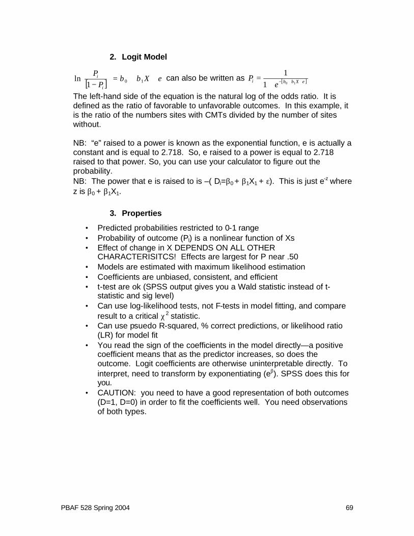
PBAF 528 Spring 2004 69
2. Logit Model
[ ] εββ ++=
−
XP
P
i
i101
ln can also be written as [ ]εββ ++−+= Xi e
P101
1
The left-hand side of the equation is the natural log of the odds ratio. It is defined as the ratio of favorable to unfavorable outcomes. In this example, it is the ratio of the numbers sites with CMTs divided by the number of sites without. NB: “e” raised to a power is known as the exponential function, e is actually a constant and is equal to 2.718. So, e raised to a power is equal to 2.718 raised to that power. So, you can use your calculator to figure out the probability. NB: The power that e is raised to is –( Di=β0 + β1X1 + ε). This is just e-z
where z is β0 + β1X1.
3. Properties
• Predicted probabilities restricted to 0-1 range • Probability of outcome (PI) is a nonlinear function of Xs • Effect of change in X DEPENDS ON ALL OTHER
CHARACTERISITCS! Effects are largest for P near .50 • Models are estimated with maximum likelihood estimation • Coefficients are unbiased, consistent, and efficient • t-test are ok (SPSS output gives you a Wald statistic instead of t-
statistic and sig level) • Can use log-likelihood tests, not F-tests in model fitting, and compare
result to a critical χ2 statistic. • Can use psuedo R-squared, % correct predictions, or likelihood ratio
(LR) for model fit • You read the sign of the coefficients in the model directly—a positive
coefficient means that as the predictor increases, so does the outcome. Logit coefficients are otherwise uninterpretable directly. To interpret, need to transform by exponentiating (eβ). SPSS does this for you.
• CAUTION: you need to have a good representation of both outcomes (D=1, D=0) in order to fit the coefficients well. You need observations of both types.
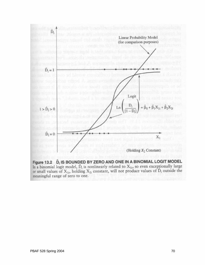
PBAF 528 Spring 2004 70

PBAF 528 Spring 2004 71
4. Logit Example
How does the elevation of the site affect the probability that it will be a site that has culturally modified trees on it? We’ll see what the probability that “site 25” (one particular parcel of land) has culturally modified trees on it. Using logit model to predict probability, proceed as follows:
zeP −+
=1
1
where z=β0 + β1X1 +…+ε: ( ) ( ) ( ) ( ) ( ) esalmonwaterbeachslopeelevationz salmonwaterbeachslopeelev ++++++= ββββββ ˆˆˆˆˆ
0
For site 25: elevation above sea level=1 slope of land=20 degrees beach=0 (0=rocky, 1=sandy) distance to water=46 distance to salmon=450 The authors fit a logit model (that is, they got the coefficients for the model, in bold below) and now we just have to fill in the characteristics of site 25. z=3.2587+(-0.3095)(1)+(0.0801)(20)+(-2.1536)(0)+(-0.0112)(46)+(0.0001)(450) z=4.081
983.01
11
1081.4 =
+=
+= −− ee
P zi
So, a site like site 25 has a 98.3% chance of having culturally modified trees—it is very likely to have them. What would the chance of having these trees be it the site were 20 feet closer to the water? You could recalculate in the form used above with water are 26 feet instead of 46, or you can take the result of above and change it by –20 times the coefficient for water. z=4.081+(-0.0112)(-20)=4.081+0.224=4.305
987.01
11
1305.4 =
+=
+= −− ee
P zi
So, if the site were 20 feet closer to the water, it would be slightly more likely to have culturally modified trees on it. The probability hasn’t changed much since the initial probability was so high. It can’t be more than 100% or 1.0. If z is very large, P approaches 1.0. If it is very negative, then P approaches 0. For this type of location, the increase is less than 1 percentage point. NB: the amount of change depends on the X values!

PBAF 528 Spring 2004 72
5. How do we interpret logit coefficients?
Coefficients are not directly interpretable. So, we have to transform them to interpret them (either as we did above or )--transform as eβ (SPSS does this). A one-unit change in X is associated with being eβ(100%) as likely to be Di=1. OR If positive sign:
eβ(100%)-(100%) more likely to be Di=1
If negative sign: 100%-eβ(100%) less likely to be Di=1
What is the impact of elevation on the probability of having a CMT or not?
Elevation is negatively associated with having a CMTs (coefficient sign). If we exponentiate the coefficient, we can interpret it: e-0.3095=.734 An additional foot of elevation is associated with being 73% as likely (or 27% less likely (100%-73%)) to have CMTs.
What is the impact of having a rocky beach in the area?
Having a rocky beach is associated with being less likely to be a CMT (negative sign). If we exponentiate the coefficient, we can interpret it: e-2.1536=.116 So, having a rocky beach is associated with being 11.6% as likely or (because a negative sign) being 88% less likely (100-11.6%) to have a CMT. If the coefficient were positive, we would subtract 1 from it. See example below.

PBAF 528 Spring 2004 73
To run a logit regression, in SPSS choose ANALYZE>REGRESSION>BINARY LOGISTIC and fill in the dependent and independent variables.
6. Some notes about logit models
• Model assumptions for OLS not a problem • Concerned about influential cases and outliers. Plot residuals to identify
those. • To compare subsets of models, can do a Likelihood Ratio (LR) test,
similar to an F-test #2. Use the –2loglikelihood statistics of nested models from the output. (LR=-2logLR-(-2logLu) =2logLu-2logLR) and compare to critical χ2 where df=number if additional regressors. If the calculated statistic is greater than the critical value, the model has explanatory power.
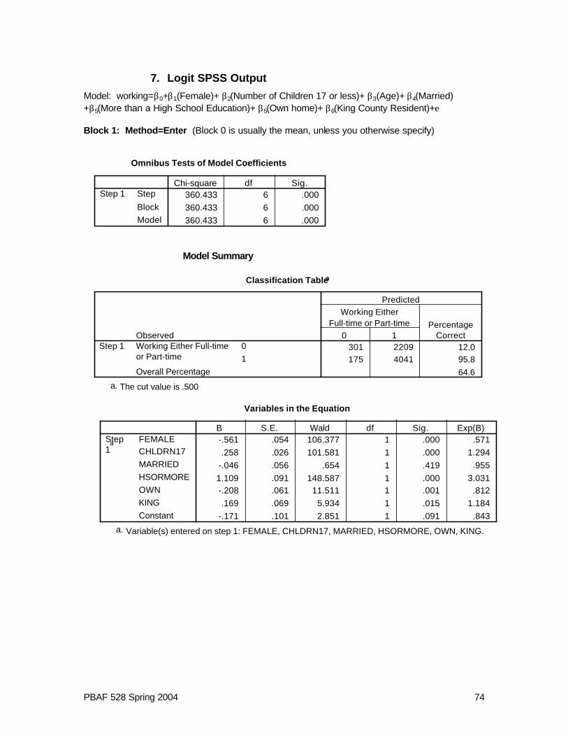
PBAF 528 Spring 2004 74
7. Logit SPSS Output
Model: working=β0+β1(Female)+ β2(Number of Children 17 or less)+ β3(Age)+ β4(Married) +β5(More than a High School Education)+ β5(Own home)+ β6(King County Resident)+e Block 1: Method=Enter (Block 0 is usually the mean, unless you otherwise specify)
Omnibus Tests of Model Coefficients
360.433 6 .000360.433 6 .000360.433 6 .000
StepBlockModel
Step 1Chi-square df Sig.
Model Summary
8526.305 .052 .071Step1
-2 Loglikelihood
Cox & SnellR Square
NagelkerkeR Square
Classification Tablea
301 2209 12.0175 4041 95.8
64.6
Observed01
Working Either Full-timeor Part-time
Overall Percentage
Step 10 1
Working EitherFull-time or Part-time Percentage
Correct
Predicted
The cut value is .500a.
Variables in the Equation
-.561 .054 106.377 1 .000 .571.258 .026 101.581 1 .000 1.294
-.046 .056 .654 1 .419 .9551.109 .091 148.587 1 .000 3.031-.208 .061 11.511 1 .001 .812.169 .069 5.934 1 .015 1.184
-.171 .101 2.851 1 .091 .843
FEMALECHLDRN17MARRIEDHSORMOREOWNKINGConstant
Step1
a
B S.E. Wald df Sig. Exp(B)
Variable(s) entered on step 1: FEMALE, CHLDRN17, MARRIED, HSORMORE, OWN, KING.a.
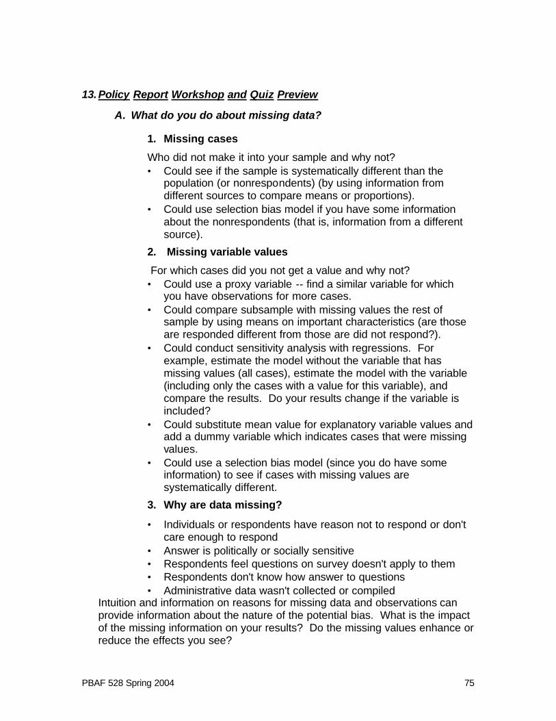
PBAF 528 Spring 2004 75
13. Policy Report Workshop and Quiz Preview
A. What do you do about missing data?
1. Missing cases
Who did not make it into your sample and why not? • Could see if the sample is systematically different than the
population (or nonrespondents) (by using information from different sources to compare means or proportions).
• Could use selection bias model if you have some information about the nonrespondents (that is, information from a different source).
2. Missing variable values
For which cases did you not get a value and why not? • Could use a proxy variable -- find a similar variable for which
you have observations for more cases. • Could compare subsample with missing values the rest of
sample by using means on important characteristics (are those are responded different from those are did not respond?).
• Could conduct sensitivity analysis with regressions. For example, estimate the model without the variable that has missing values (all cases), estimate the model with the variable (including only the cases with a value for this variable), and compare the results. Do your results change if the variable is included?
• Could substitute mean value for explanatory variable values and add a dummy variable which indicates cases that were missing values.
• Could use a selection bias model (since you do have some information) to see if cases with missing values are systematically different.
3. Why are data missing?
• Individuals or respondents have reason not to respond or don't care enough to respond
• Answer is politically or socially sensitive • Respondents feel questions on survey doesn't apply to them • Respondents don't know how answer to questions • Administrative data wasn't collected or compiled
Intuition and information on reasons for missing data and observations can provide information about the nature of the potential bias. What is the impact of the missing information on your results? Do the missing values enhance or reduce the effects you see?
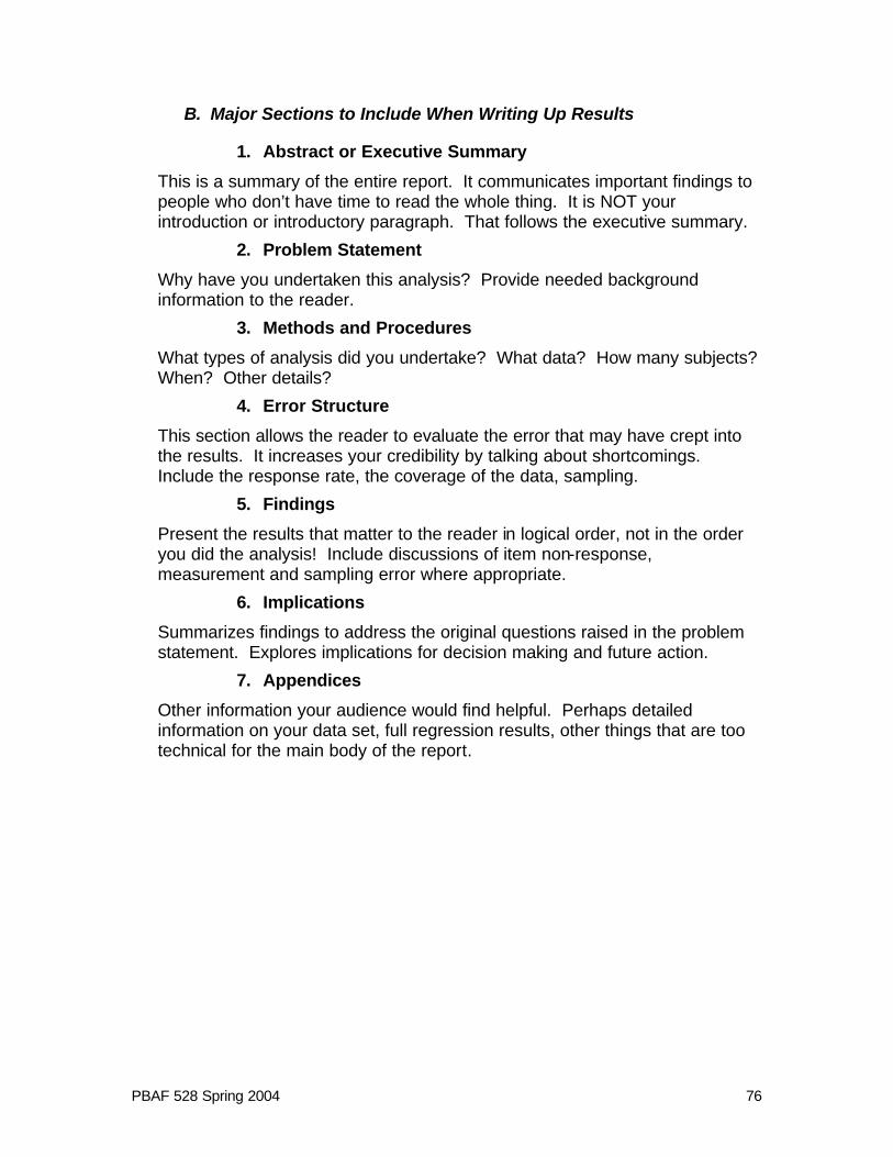
PBAF 528 Spring 2004 76
B. Major Sections to Include When Writing Up Results
1. Abstract or Executive Summary
This is a summary of the entire report. It communicates important findings to people who don’t have time to read the whole thing. It is NOT your introduction or introductory paragraph. That follows the executive summary.
2. Problem Statement
Why have you undertaken this analysis? Provide needed background information to the reader.
3. Methods and Procedures
What types of analysis did you undertake? What data? How many subjects? When? Other details?
4. Error Structure
This section allows the reader to evaluate the error that may have crept into the results. It increases your credibility by talking about shortcomings. Include the response rate, the coverage of the data, sampling.
5. Findings
Present the results that matter to the reader in logical order, not in the order you did the analysis! Include discussions of item non-response, measurement and sampling error where appropriate.
6. Implications
Summarizes findings to address the original questions raised in the problem statement. Explores implications for decision making and future action.
7. Appendices
Other information your audience would find helpful. Perhaps detailed information on your data set, full regression results, other things that are too technical for the main body of the report.

PBAF 528 Spring 2004 77
C. Quiz Preview
1. Continuous Dependent Variables--OLS
a) Determine the significance of coefficients
b) R2 and adjusted R2
c) Coefficient interpretation, including dummy variables, interactions, and nonlinear functional form
d) Hypothesis testing with F-tests.
e) Prediction with regression models
2. Dummy Dependent Variables
a) Contingency Tables and Chi-Square
b) Logit Models
(1) Determine the significance of coefficients with t-test or Wald Chi-Square statistic. (2) Calculate predicted probabilities (3) Interpret regression coefficients
14. Quiz 2
15. Policy Report Question and Answer Session

PBAF 528 Spring 2004 78
16. So, you want to collect data What type of data collection is appropriate?
A. When would you use Qualitative Methods?
When you: • want to understand processes, social phenomena and dynamics in their
natural setting. • want to learn about the depth of a problem, an intervention. • can’t get a large enough sample of a population to perform a quantitative
analysis. Included most often in policy and management applications: Focus groups Case studies Ethnography Participatory Action Research
B. When is a Survey Appropriate?
When you: • need to describe the characteristics of a large population. • want direct measurement of attributes, attitudes, and orientations,
opinion
C. Types of Surveys
1. Self-administered questionnaires
mail survey, administer to a group, home delivery
a) Some advice:
• Make it easy to return using self mailers, booklets, stamped envelops/business reply
• Send it out as if that each respondent is the only on receiving it--No bulk rate!
• Always include a paragraph or letter explaining they study and why it is in the interest of the respondent to reply!
• FOLLOW UP: A thank you letter, another survey at 2 week intervals (3 waves total)
b) Problems
• Low return rate • Incomplete responses • Confusion when writing answers down • Need to monitor returns to evaluate nonresponse bias.
But if confidential, a problem
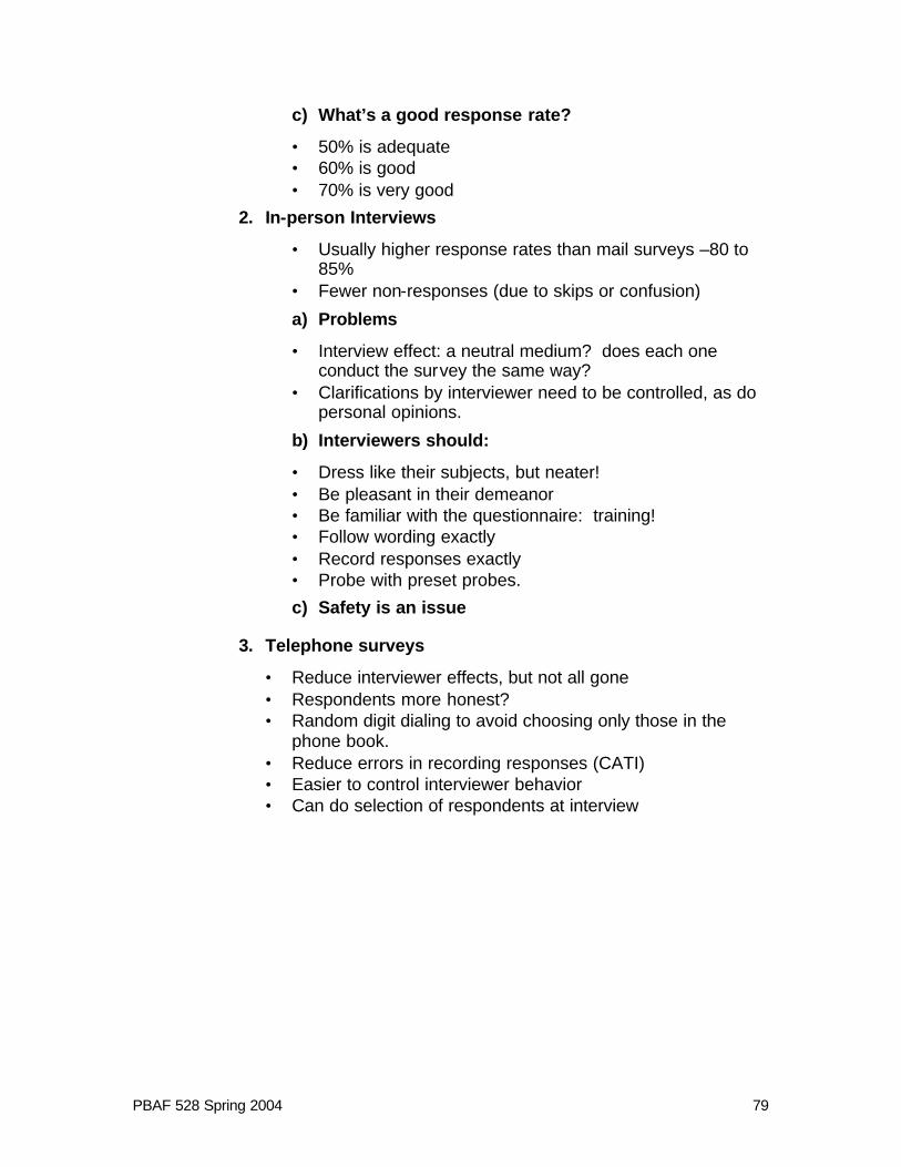
PBAF 528 Spring 2004 79
c) What’s a good response rate?
• 50% is adequate • 60% is good • 70% is very good
2. In-person Interviews
• Usually higher response rates than mail surveys –80 to 85%
• Fewer non-responses (due to skips or confusion)
a) Problems
• Interview effect: a neutral medium? does each one conduct the survey the same way?
• Clarifications by interviewer need to be controlled, as do personal opinions.
b) Interviewers should:
• Dress like their subjects, but neater! • Be pleasant in their demeanor • Be familiar with the questionnaire: training! • Follow wording exactly • Record responses exactly • Probe with preset probes.
c) Safety is an issue
3. Telephone surveys
• Reduce interviewer effects, but not all gone • Respondents more honest? • Random digit dialing to avoid choosing only those in the
phone book. • Reduce errors in recording responses (CATI) • Easier to control interviewer behavior • Can do selection of respondents at interview
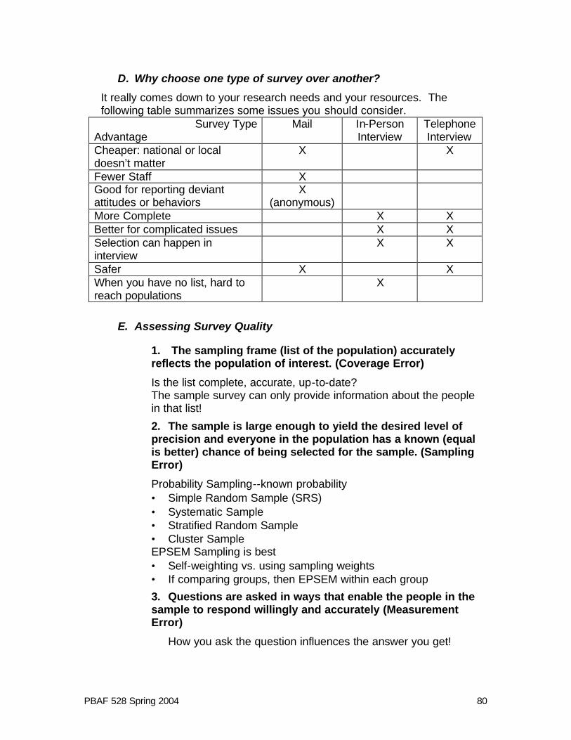
PBAF 528 Spring 2004 80
D. Why choose one type of survey over another?
It really comes down to your research needs and your resources. The following table summarizes some issues you should consider.
Survey Type Advantage
Mail In-Person Interview
Telephone Interview
Cheaper: national or local doesn’t matter
X X
Fewer Staff X Good for reporting deviant attitudes or behaviors
X (anonymous)
More Complete X X Better for complicated issues X X Selection can happen in interview
X X
Safer X X When you have no list, hard to reach populations
X
E. Assessing Survey Quality
1. The sampling frame (list of the population) accurately reflects the population of interest. (Coverage Error)
Is the list complete, accurate, up-to-date? The sample survey can only provide information about the people in that list!
2. The sample is large enough to yield the desired level of precision and everyone in the population has a known (equal is better) chance of being selected for the sample. (Sampling Error)
Probability Sampling--known probability • Simple Random Sample (SRS) • Systematic Sample • Stratified Random Sample • Cluster Sample EPSEM Sampling is best • Self-weighting vs. using sampling weights • If comparing groups, then EPSEM within each group
3. Questions are asked in ways that enable the people in the sample to respond willingly and accurately (Measurement Error)
How you ask the question influences the answer you get!

PBAF 528 Spring 2004 81
• Question structure can influence the responses you get, as can order.
• How specific? • Will it produce credible information? • Will R be able to answer? • Will R be willing to answer? • Do you want to know about
behavior or attributes attitudes or beliefs
Interviewer error can cause problems, as can misunderstandings by respondents.
4. The characteristics of people selected in the sampling process but who do not participate in the survey are similar to the characteristics of those who do. (nonresponse error)2
• More than a small number of people who were selected in the sample are not interviewed, either because they cannot be reached or refuse to participate
• Nonrespondents are different from respondents in a way that pertains to the study focus.
• A high response rate helps avoid this: Mail: 50% or more, 70% better In-person or Telephone: 80-75% The last few are the most expensive!
F. Survey Ethics and Psychology
1. Why would someone (anyone?) participate in a survey?
2. What sorts of questions are appropriate for different survey modalities?
3. Pretest, pretest, pretest.
4. Confidentiality or not?
5. Human Subjects
If you plan to do your own survey, I highly recommend: Priscilla Salant and Don A. Dillman. 1994. How to Conduct Your Own Survey (New York:John Wiley and Sons).
2 Salant and Dillman.1994. How to Conduct Your Own Survey (New York: John Wiley and Sons, Inc.).

PBAF 528 Spring 2004 82
17. Evaluating Empirical Studies What unresolved questions?
18. Discussion of Projects, Course Evaluations