class progress - smu
TRANSCRIPT

1Physics 3340 - Fall 2017
Class Progress
Basics of Linux, gnuplot, CVisualization of numerical dataRoots of nonlinear equations (Midterm 1)Solutions of systems of linear equationsSolutions of systems of nonlinear equationsMonte Carlo simulationInterpolation of sparse data pointsNumerical integration (Midterm 2)Solutions of ordinary differential equations

2Physics 3340 - Fall 2017
Helmholtz Coil for Uniform Magnetic Field

3Physics 3340 - Fall 2017
Magnetic Field Along Axis of a Single Coil
y
z
x
R = coil radius
current I
R
Bz(z) = z component of magnetic
field at coordinate z on the axis of symmetry
B z (z) =μ0 I R2
2(R2+z2)32

4Physics 3340 - Fall 2017
Magnetic Field on Axis of a Helmholtz Coil
y
z
x
R = coil radiusD = z distance of the plane of each coil from the z=0 planeD = R/2 for best uniform fields
D
Dcurrent I
R
(Region of approximately uniform magnetic field in z direction)
current I

5Physics 3340 - Fall 2017
Magnetic Field on Axis of a Helmholtz CoilR=10cm D=5cm I=1A
0
2x10⁻⁶
4x10⁻⁶
6x10⁻⁶
8x10⁻⁶
1x10⁻⁵
1.2x10⁻⁵
-0.1 -0.05 0 0.05 0.1
Z c
om
po
ne
nt o
f ma
gn
etic
fie
ld (
T)
Z coordinate (m)
Both coilsLower coilUpper coil

6Physics 3340 - Fall 2017
Magnetic Field on Axis of a Helmholtz CoilR=10cm D=6cm I=1A
0
2x10⁻⁶
4x10⁻⁶
6x10⁻⁶
8x10⁻⁶
1x10⁻⁵
1.2x10⁻⁵
-0.1 -0.05 0 0.05 0.1
Z c
om
po
ne
nt o
f ma
gn
etic
fie
ld (
T)
Z coordinate (m)
Both coilsLower coilUpper coil

7Physics 3340 - Fall 2017
Magnetic Field on Axis of a Helmholtz CoilR=10cm D=4cm I=1A
0
2x10⁻⁶
4x10⁻⁶
6x10⁻⁶
8x10⁻⁶
1x10⁻⁵
1.2x10⁻⁵
-0.1 -0.05 0 0.05 0.1
Z c
om
po
ne
nt o
f ma
gn
etic
fie
ld (
T)
Z coordinate (m)
Both coilsLower coilUpper coil

8Physics 3340 - Fall 2017
Two-Dimensional Wave Diffraction Patterns
y
z
x
z=-D0
z=0
z=D1
Aperture
ObservationScreen
R
(x,y)
r1
θ1
(x1,y
1)
Point source
d1
d0
(x0,y
0)

9Physics 3340 - Fall 2017
Review of PhasorsConsider any physical system described by a linear second order ODE with constant coefficients, driven by a sinusoid at a fixed frequency and a reference phase:
−ω2 Aei ϕ+ a iω Ae iϕ+ b Aei ϕ=c
Plug prototype solution back into ODE:
dx2
dt 2+ a dx
dt+ b x=c eiω t
Look only for a solution in the form of a steady state sinusoid with unknown amplitude and phase. Form a prototype solution of the form:
x=Aei (ω t−ϕ)=Aei ϕeiω t
−ω2 Aei ϕe iω t+ a iω Ae iϕeiω t+ b Aei ϕe iω t=c e iω t
Cancel eiωt factors:
Second order ODE has been transformed into a complex algebraic equation AeiΦ is called the “phasor” of the solution x

10Physics 3340 - Fall 2017
Phasor Method for Wave Interference
Point source 2
Observation point
Point source 1
E field at observation point=∑ E j from point source jAssume uniform polarization,so for instance E j=E jx xE jx=E j0 e
i t−=E j0 eiei t
E j0 ei is the 'phasor' from source j
is due to path length differencesd
2
d1

11Physics 3340 - Fall 2017
Diffraction Pattern from Single Point Source
R=1D
1=20
D0=20
λ=0.2x
0=0
y0=0

12Physics 3340 - Fall 2017
Diffraction Pattern from Single Point Source
R=1D
1=20
D0=20
λ=0.2x
0=3
y0=0

13Physics 3340 - Fall 2017
Diffraction Pattern from Single Point Source
R=1D
1=20
D0=20
λ=0.2x
0=-3
y0=0
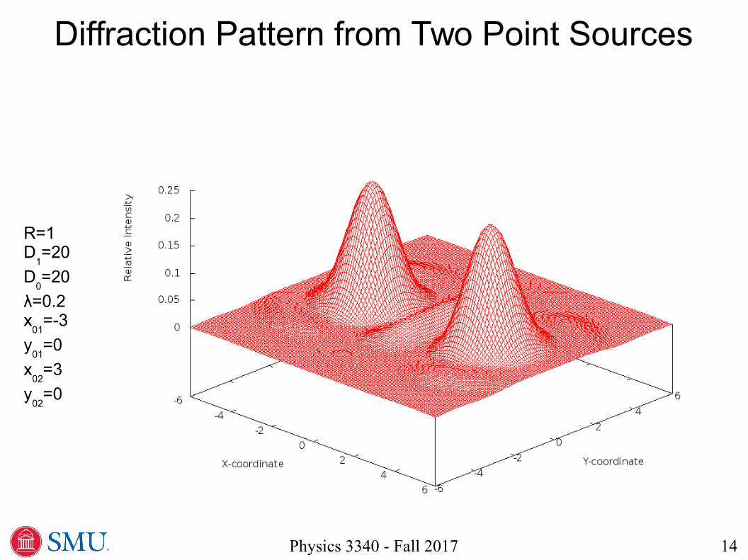
14Physics 3340 - Fall 2017
Diffraction Pattern from Two Point Sources
R=1D
1=20
D0=20
λ=0.2x
01=-3
y01
=0
x02
=3
y02
=0

15Physics 3340 - Fall 2017
Diffraction Pattern from Two Point Sources
R=1D
1=20
D0=20
λ=0.2x
01=-1
y01
=0
x02
=1
y02
=0

16Physics 3340 - Fall 2017
Diffraction Pattern from Two Point Sources
R=1D
1=20
D0=20
λ=0.2x
01=-2
y01
=0
x02
=2
y02
=0

17Physics 3340 - Fall 2017
Simulation of the Poisson Spot
RDISC
=2D
1=20
D0=20
λ=0.2x
0=0
y0=0

18Physics 3340 - Fall 2017
One-Dimensional Wave Diffraction Patterns
y
x
y=-D0
x=W/2
y=D1
Aperture
ObservationScreen
x
x1
Point source
d1
d0
x0
y=0
x=0
x=-W/2

19Physics 3340 - Fall 2017
1-Dimensional Diffraction Pattern from Single Point Source
W=1D
1=20
D0=20
λ=0.2x
0=0
0
0.1
0.2
0.3
0.4
0.5
0.6
0.7
0.8
0.9
1
-10 -5 0 5 10
Re
lativ
e In
ten
sity
X-coordinate

20Physics 3340 - Fall 2017
1-Dimensional Diffraction Pattern from Single Point Source
W=1D
1=20
D0=20
λ=0.2x
0=-5
0
0.1
0.2
0.3
0.4
0.5
0.6
0.7
0.8
0.9
1
-10 -5 0 5 10
Re
lativ
e In
ten
sity
X-coordinate

21Physics 3340 - Fall 2017
1-Dimensional Diffraction Pattern from Single Point Source
W=1D
1=20
D0=20
λ=0.2x
0=5
0
0.1
0.2
0.3
0.4
0.5
0.6
0.7
0.8
0.9
1
-10 -5 0 5 10
Re
lativ
e In
ten
sity
X-coordinate

22Physics 3340 - Fall 2017
1-Dimensional Diffraction Pattern from Two Point Sources
W=1D
1=20
D0=20
λ=0.2x
01=5
x02
=-5
0
0.2
0.4
0.6
0.8
1
1.2
1.4
-10 -5 0 5 10
Re
lativ
e In
ten
sity
X-coordinate

23Physics 3340 - Fall 2017
1-Dimensional Diffraction Pattern from Two Point Sources
W=1D
1=20
D0=20
λ=0.2x
01=2
x02
=-2
0
0.2
0.4
0.6
0.8
1
1.2
1.4
1.6
1.8
-10 -5 0 5 10
Re
lativ
e In
ten
sity
X-coordinate

24Physics 3340 - Fall 2017
1-Dimensional Diffraction Pattern from Two Point Sources
W=1D
1=20
D0=20
λ=0.2x
01=3
x02
=-3
0
0.1
0.2
0.3
0.4
0.5
0.6
0.7
-10 -5 0 5 10
Re
lativ
e In
ten
sity
X-coordinate

25Physics 3340 - Fall 2017
Plotting Vectors with gnuplot
plot 'efield1.dat' using 1:2 with lines
Column with Y coordinate
Column with X coordinate
plot 'efield1.dat' using 1:2:3:4 with vectors
Column with starting Y coordinate
Column with starting X coordinate
Column with Y distance
Column with X distance
plot 'efield1.dat' using 1:2 with points
Another plot mode:
We have used:

26Physics 3340 - Fall 2017
Electric Field Vectors for Dipole
-25
-20
-15
-10
-5
0
5
10
15
20
25
-25 -20 -15 -10 -5 0 5 10 15 20 25

27Physics 3340 - Fall 2017
Electric Field Vectors for Quadrapole
-25
-20
-15
-10
-5
0
5
10
15
20
25
-25 -20 -15 -10 -5 0 5 10 15 20 25

28Physics 3340 - Fall 2017
Electric Field Vectors for Example Arbitrary Charges
-25
-20
-15
-10
-5
0
5
10
15
20
25
-25 -20 -15 -10 -5 0 5 10 15 20 25

29Physics 3340 - Fall 2017
C Code for Mapping Electric Field Vectors
xstop = xstop + xinc * 0.5; ystop = ystop + yinc * 0.5; rtest = 1.0e-6 * (xinc*xinc + yinc*yinc); x = xstart; while (((xinc > 0.0) && (x < xstop)) || ((xinc < 0.0) && (x > xstop))) { y = ystart; while (((yinc > 0.0) && (y < ystop)) || ((yinc < 0.0) && (y > ystop))) { ex = 0.0; ey = 0.0; i = 0; while (i < n) { rsq = (x-xi[i])*(x-xi[i]) + (y-yi[i])*(y-yi[i]); if (rsq < rtest) break; r = sqrt(rsq); ex += qi[i] * (x-xi[i]) / (r * rsq); ey += qi[i] * (y-yi[i]) / (r * rsq); i++; } if (i >= n) { emag = sqrt(ex*ex + ey*ey); vx = xinc * ex / emag; vy = yinc * ey / emag; printf("%.8g %.8g %.8g %.8g\n",x-0.5*vx,y-0.5*vy,vx,vy); } y = y + yinc; } x = x + xinc; }
Loop over n charges.double array qi[] hold each charge q
i and
double arrays xi[] and yi[] hold x
i and y
i coordinates

30Physics 3340 - Fall 2017
Classical Electric Field Lines
Note that the vectors plotted by this method only record the direction of the E field vector at an array of sampled points. These are not quite equivalent to the classical field lines, which convey both the direction of the field and its magnitude from the density of drawn lines.

31Physics 3340 - Fall 2017
Classical Electric Equipotential Lines
A simple modification of this algorithm can be used to plot a sampling of the direction of the electric equipotential lines. At a given point, field lines and equipotential lines will have slopes that are negative reciprocals of each other. Again, no magnitude information is present, only direction.

32Physics 3340 - Fall 2017
Equipotential Vectors for Example Arbitrary Charges
-25
-20
-15
-10
-5
0
5
10
15
20
25
-25 -20 -15 -10 -5 0 5 10 15 20 25
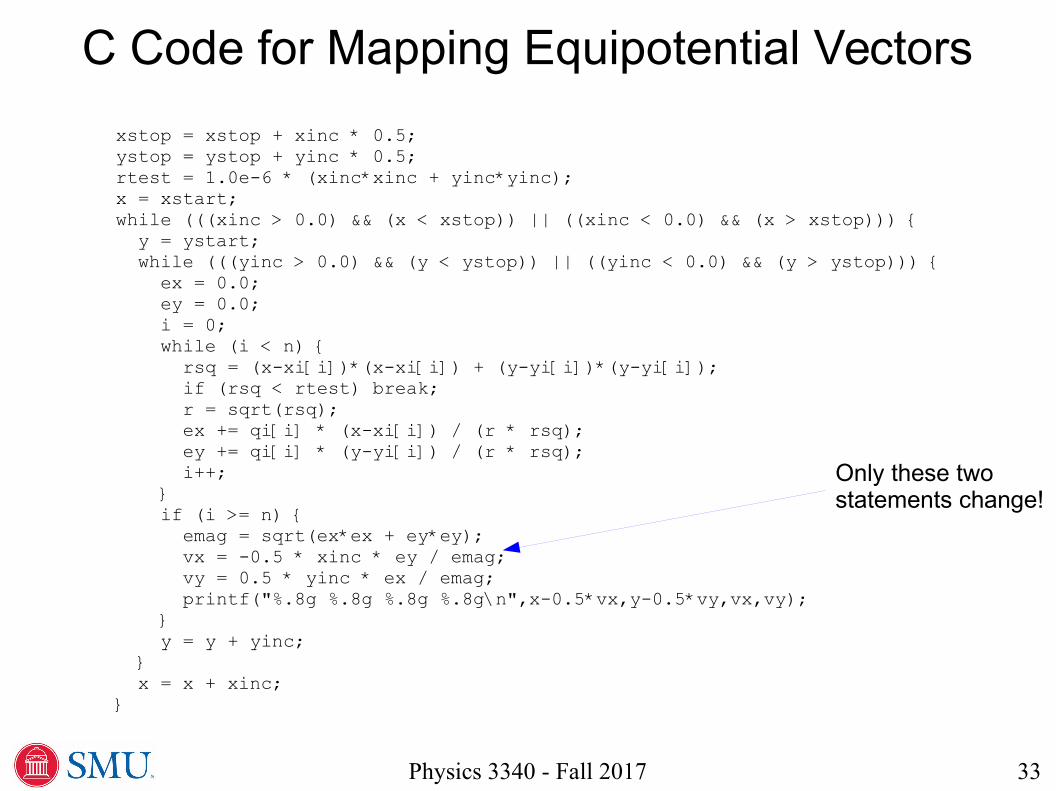
33Physics 3340 - Fall 2017
C Code for Mapping Equipotential Vectors
xstop = xstop + xinc * 0.5; ystop = ystop + yinc * 0.5; rtest = 1.0e-6 * (xinc*xinc + yinc*yinc); x = xstart; while (((xinc > 0.0) && (x < xstop)) || ((xinc < 0.0) && (x > xstop))) { y = ystart; while (((yinc > 0.0) && (y < ystop)) || ((yinc < 0.0) && (y > ystop))) { ex = 0.0; ey = 0.0; i = 0; while (i < n) { rsq = (x-xi[i])*(x-xi[i]) + (y-yi[i])*(y-yi[i]); if (rsq < rtest) break; r = sqrt(rsq); ex += qi[i] * (x-xi[i]) / (r * rsq); ey += qi[i] * (y-yi[i]) / (r * rsq); i++; } if (i >= n) { emag = sqrt(ex*ex + ey*ey); vx = -0.5 * xinc * ey / emag; vy = 0.5 * yinc * ex / emag; printf("%.8g %.8g %.8g %.8g\n",x-0.5*vx,y-0.5*vy,vx,vy); } y = y + yinc; } x = x + xinc; }
Only these two statements change!

34Physics 3340 - Fall 2017
Examples of Optical Glare
(Vacuum tube arithmetic unit and magnetic drum memory from the Univac 1, on display at the Deutches Museum of Technology, Munich, Germany)
Glare is the reflected room light off of an intervening plexiglass protective sheet.Reflections occur at the interface between two materials of different refractive indices.

35Physics 3340 - Fall 2017
Computing Another Kind of Glare: a Rainbow

36Physics 3340 - Fall 2017
Rene Descartes Graphical Derivation
“I took my pen and made an accurate calculation of the paths of the rays which fall on the different points of a globe of water to determine at which angles, after two refractions and one or two reflections they will come to the eye, and I then found that after one reflection and two refractions there are many more rays which can be seen at an angle of from forty-one to forty-two degrees than at any smaller angle; and that there are none which can be seen at a larger angle"

37Physics 3340 - Fall 2017
Calculating Reflection and Refraction Angles
θi1
θr1
θ12
θn2
θ23
θ12
θi2
θr2
(x0,y
0)
θ23
θi3
θn3θ
out
θr3
(x2,y
2)
(x1,y
1)
(x3,y
3)
Spherical water raindrop cross section, index of refraction n
Output ray
Horizontal input ray
Radius r
(0,0)

38Physics 3340 - Fall 2017
Calculating Reflection and Refraction Angles
x1=−√r2− y02 y1=y 0 θi1=arctan (∣y1
x1∣)
Snell's law: θr1=arcsin ( 1n
sin (θi1))θ12=θi1−θr1 m12= tan (−θ12)
x 2=x1(m12
2 −1)−2m12 y1
m122 +1
y 2= y1+m12(x2−x1)
θn2=arctan ( y2
x2) θi2=θn2+θ12 θ23=θn2+θi2=2θn2+θ12 m23= tan (θ23)
x3=x2(m23
2 −1)−2m23 y2
m232 +1
y3= y2+m23(x3−x 2)
θn3=arctan ( y3
x3) θi3=θn3−θ23
Snell's law: θr3=arcsin (n⋅sin (θi3))θout=θn3−θr3

39Physics 3340 - Fall 2017
Reflection and Refractions through a Raindrop
Incoming violet light λ=400nm
Reflected light rays to observer on ground
Spherical raindrop of water, n=1.339at λ=400nm
Many reflection paths bundled at an angle of about 40˚ below horizontal
-3
-2.5
-2
-1.5
-1
-0.5
0
0.5
1
-2 -1.5 -1 -0.5 0 0.5 1 1.5 2

40Physics 3340 - Fall 2017
Reflection and Refractions through a Raindrop
Incoming red light λ=700nm
Reflected light rays to observer on ground
Spherical raindrop of water, n=1.331at λ=700nm
Many reflection paths bundled at an angle of about 42˚ below horizontal
-3
-2.5
-2
-1.5
-1
-0.5
0
0.5
1
-2 -1.5 -1 -0.5 0 0.5 1 1.5 2

41Physics 3340 - Fall 2017
1.33 1.331
1.332 1.333
1.334 1.335
1.336 1.337
1.338 1.339
Refractive index
0 0.1
0.2 0.3
0.4 0.5
0.6 0.7
0.8 0.9
1Incident Y coordinate
0
5
10
15
20
25
30
35
40
45
Ou
tpu
t an
gle
(d
eg
ree
s )
Output Angle Relative to Horizontal
Angle reaches a maximum, which concentrates much of the output energy around 40˚ - 42˚
λ=700nm (red)
λ=400nm (violet)

42Physics 3340 - Fall 2017
Total Effect of Many Raindrops is a Rainbow
Observer
Red light appears on the top, violet light appears on the bottom
Incident white sunlight
Many raindrops in rainfall

43Physics 3340 - Fall 2017
Wave Packets for Quantum Mechanics
d2 ψ(x)d x2 =−2m
ℏ2 [E−V (x) ] ψ(x)
Solutions of the time-independent Schrödinger equation in one dimension
in regions where particles are free to move and not subject to forces, or
V (x)=0 and E>0are of the form
ψ(x)=A e+i(kx−ω t )+Be−i(kx+ω t)
ψ(x)=A e+ikx+Be−ikx
which makes the complete solution including the time dependence
where k= pℏ
and ω= Eℏ
so the relationship between ω and k is
ω=ℏ
2mk2

44Physics 3340 - Fall 2017
Wave Packets for Quantum Mechanics
ψ(x)=∫ A (k )ψk (x)dk
A single wave solution is associated with a continuous flux of particles in the positive or negative x direction, with momentum p and energy E.
Solutions that are linear combinations of multiple waves form wave packets that are associated with single particles.
A (k )=e−a2(k−k0)2
Look at Gaussian wave packets where
ψ(x)=∑k
Ak ψk (x)
Or in the continuous limit
Ak=e−a2(k−k0)2
Or in the continuous limit

45Physics 3340 - Fall 2017
Distribution of Wave Numbers
0
0.2
0.4
0.6
0.8
1
40 45 50 55 60
A(k
)
k
Gaussian wavepacket
a=1a=2
a=0.5

46Physics 3340 - Fall 2017
Corresponding Spatial Wave Distribution
0
200
400
600
800
1000
1200
1400
-15 -10 -5 0 5 10 15
Psi
(X)
X
Gaussian wavepacket
a=1a=2
a=0.5
47Physics 3340 - Fall 2017
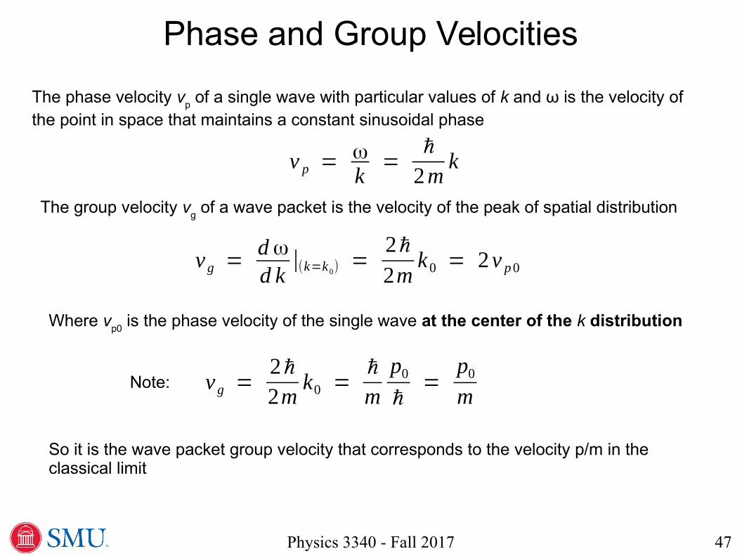
Phase and Group Velocities
The phase velocity vp of a single wave with particular values of k and ω is the velocity of
the point in space that maintains a constant sinusoidal phase
v g =2ℏ2m
k0 =ℏm
p0
ℏ=
p0
m
The group velocity vg of a wave packet is the velocity of the peak of spatial distribution
v p = ωk
=ℏ
2mk
Where vp0
is the phase velocity of the single wave at the center of the k distribution
v g = d ωd k
|(k=k0) =2ℏ2m
k0 = 2v p0
Note:
So it is the wave packet group velocity that corresponds to the velocity p/m in the classical limit

48Physics 3340 - Fall 2017
Discrete Approximation to Gaussian Packet
-20
-15
-10
-5
0
5
10
15
20
-15 -10 -5 0 5 10 15
Psi
(X)
X
Gaussian wavepacket, a=1
RealImaginary
49Physics 3340 - Fall 2017
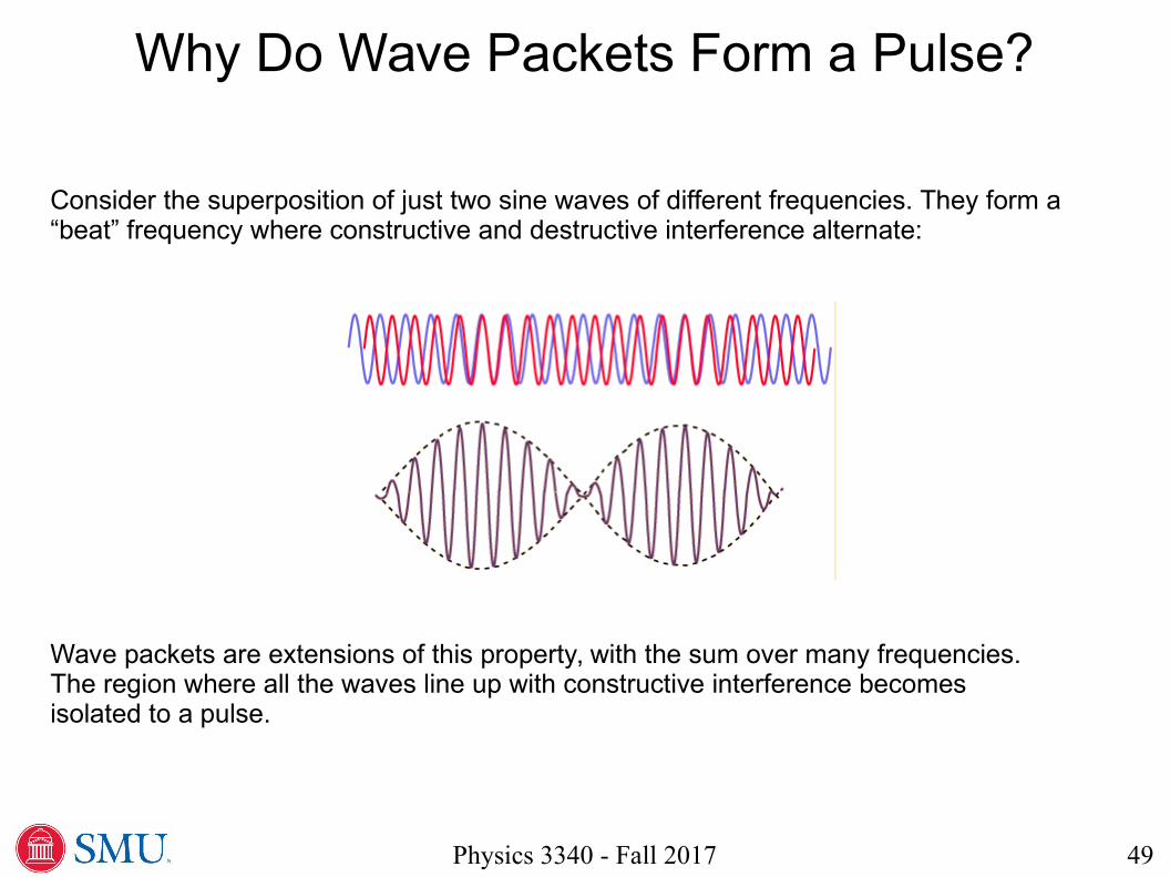
Why Do Wave Packets Form a Pulse?
Consider the superposition of just two sine waves of different frequencies. They form a “beat” frequency where constructive and destructive interference alternate:
Wave packets are extensions of this property, with the sum over many frequencies. The region where all the waves line up with constructive interference becomes isolated to a pulse.

50Physics 3340 - Fall 2017
Quality of Discrete Approximations
0
10
20
30
40
50
60
-15 -10 -5 0 5 10 15
Ma
gn
itud
e S
qu
are
d o
f Psi
( x)
X
Gaussian Wave Packet, n=number of component waves
n=1n=3n=5n=7n=9
n=11n=13n=17

51Physics 3340 - Fall 2017
Group Velocity versus Phase Velocity
-20
-15
-10
-5
0
5
10
15
20
-10 -5 0 5 10 15 20
Psi
(X)
X
Gaussian wavepacket, a=1, time=5, phase velocity=1
RealImaginary

52Physics 3340 - Fall 2017
Uncertainty Principle of Wave Packets
Δ k2=[k−k ]2=∫ A (k)2[k−k ]2 dk
∫ A (k)2 dk
Δ x2=[x−x ]2=∫ψ(x)2[x−x ]2 dx
∫ψ(x)2dx
then Δ x2⋅Δ k2≥14