Class-Size Effects in School Systems Around the World: Evidence from Between-Grade

Variation in TIMSS

Ludger Wößmann and Martin R. West

PEPG/02-02

Class-Size Effects in School Systems Around the World: Evidence from Between-Grade Variation in TIMSS

Ludger Wößmann Kiel Institute for World Economics

Duesternbrooker Weg 120 24100 Kiel, Germany

Phone: (+49) 431-8814 497 E-mail: woessmann@ifw.uni-kiel.de

Martin R. West Program on Education Policy and Governance

Harvard University 79 J. F. Kennedy Street, Taubman 306

Cambridge, MA 02138, USA Phone: (+1) 617-496 5488

E-mail: mrwest@fas.harvard.edu

March 26, 2002

Class-Size Effects in School Systems Around the World: Evidence from Between-Grade Variation in TIMSS∗

Abstract

We estimate the effect of class size on student performance in 18 countries, combining school fixed effects and instrumental variables to identify random class-size variation between two adjacent grades within individual schools. Conventional estimates of class-size effects are shown to be severely biased by the non-random placement of students between and within schools. Smaller classes exhibit beneficial effects only in countries with relatively low teacher salaries. While we find sizable beneficial effects of smaller classes in Greece and Iceland, the possibility of even small effects is rejected in Japan and Singapore. In 11 countries, we rule out large class-size effects.

∗ We would like to thank Sveinn Agnarsson (University of Iceland) and George Psacharopoulos

(University of Athens) for sharing their knowledge of their respective countries’ school systems, and Paul E. Peterson and Erich Gundlach for their comments on the manuscript. One author would like to thank the Program on Education Policy and Governance (PEPG) at the Kennedy School of Government, Harvard University, and the National Bureau of Economic Research (NBER) for their hospitality during his stay in Cambridge, Mass., during which the main work on this paper was completed.

I. Introduction

School systems around the world differ in many respects. Important sources of variation include

examination systems, the existence of high-stakes incentives for students and teachers, the

provision of remedial instruction for lagging students or of enrichment classes for outstanding

students, the level and allocation of resources, the quality of the teaching force, and average class

size. Given these differences, it is not obvious that findings from any particular school system

translate directly into general principles for all systems. Although the effect of class size on

student achievement in the United States has recently been the subject of a great deal of research,

the U.S. findings simply may not generalize to school systems in other parts of the world with

distinctive institutional configurations. This paper explores this possibility by providing

estimates of class-size effects in 18 education systems scattered across four continents.

The central problem in estimating class-size effects is that placement decisions made by

parents and schools obscure the causal relationship between class size and student performance.

For example, parents may place children in schools with bigger or smaller class sizes on the

basis of their educational performance; administrative rules may track students into different

schools depending on their achievement; and individual educators may sort students within a

school into differently sized classes according to their behavior or demonstrated academic

potential. As a result, naïve estimates of education production functions may be biased both by

endogeneity of class size with respect to student performance and by omitted variables.

Estimating “true” class-size effects, i.e. the causal effect of class size on student performance,

thus requires an identification strategy that restricts the analysis to exogenous variations in class

size, thereby allowing for the causal class-size effect to be disentangled from the effects of

sorting.

In principle, two such strategies are available. The first is to conduct an experiment, using

random assignment of students to classrooms to ensure that all variation in class size is

exogenous. The second is to adopt a quasi-experimental approach in which instrumental variable

(IV) estimates are used to restrict the analysis to that part of the total variation in class size that is

exogenous to student achievement.

1

Evidence from the one large-scale random-assignment experiment on class-size effects, the

Tennessee Student/Teacher Achievement Ratio experiment (“Project STAR”), has been analyzed

both in terms of its initial impact on student achievement (Krueger 1999) and in its longer-term

consequences for academic progress (Krueger and Whitmore 2001). Unfortunately, however, the

validity of this experiment may actually have been undermined by specific decentralized

placement decisions; non-random parental choices prior to the start of the experiment – e.g. not

to send their children to participating schools if they were assigned to larger classes – cannot be

ruled out and would bias any estimate of class-size effects. Several other issues of design and

implementation of Project STAR also call into question the validity of its results (Hanushek

1999). Furthermore, any experiment suffers from the so-called “Hawthorne effect” in that

participants are aware that they are being evaluated, and may respond by increasing their effort.

Knowledge of one’s participation in an experiment can also alter the prevailing incentive

conditions in important ways. For example, the schools participating in Project STAR may have

realized that their future resource endowments would be affected by the outcome of the

experiment, and may have adjusted their behavior accordingly (Hoxby 2000). In short, the use of

randomized experiments to assess the effects of class size has intrinsic problems, and the

implementation of the one major class-size experiment seems to have been less than optimal.

And it must be recalled that we have evidence from only one experiment, conducted in a single

U.S. state in the mid-eighties. The near universal popularity of country music notwithstanding,

the situation in Tennessee simply may not be representative of school systems in other parts of

the world.

Studies using quasi-experimental evidence also have important disadvantages. Principle

among them is the need to examine rather specific variations in class size that make it possible to

disentangle the causal effect of class size on student achievement from the results of sorting. As

a consequence, studies using this kind of identification strategy are also only available for a few

countries and situations. Angrist and Lavy (1999) exploit a specific rule on maximum class size

in Israel to extract presumably exogenous variation in Israeli class sizes. While this identification

strategy excludes class-size variations due to student assignments within a school, it is not

immune to bias from parental residential choice. Moreover, they are only able to analyze the

effects of variation in class size between 20 and 40 students, which may not be the range most of

interest to policy-makers in many countries. Case and Deaton (1999) identify class-size effects

2

by looking at data on black students in South Africa during apartheid, arguing that the variation

in class sizes for black students was largely exogenous, because the black population at this time

had neither freedom of residential choice nor control over their schools’ endowments. But the

South African school system during apartheid was obviously unique in its institutional

configuration, and was characterized by district-average class sizes of up to 80 students. It is

therefore unclear whether the results are relevant to more advanced countries. Hoxby (2000)

exploits variation over time in student enrollments due to random fluctuations in the timing of

births and district rules regarding maximum or minimum class sizes to identify exogenous

variation in class sizes, applying this approach to elementary schools in the U.S. state of

Connecticut. Unfortunately, her identification strategies require a long panel of rich data and

have yet to be applied in other contexts.

In this paper, we use the international database of the Third International Mathematics and

Science Study (TIMSS) and develop a new identification strategy that provides unbiased

estimates of the effects of class size on student achievement in a host of school systems from all

over the world. The TIMSS database provides data on representative samples of students in the

two adjacent grades with the highest share of thirteen-year-old students from about 40 countries,

18 of which have data rich enough to support the implementation of our identification strategy.

Our identification strategy is designed to take advantage of two unique characteristics of this

database. Specifically, it exploits the fact that the TIMSS database contains information on the

performance and class size of students in two adjacent grades of each school taking the same

achievement test, as well as on the average class size in each grade of each school.

In a nutshell, our identification strategy uses the part of the between-grade difference in class

size in a school that reflects differences in the school’s average class size between the two grades

to predict that part of the between-grade difference in student performance that is idiosyncratic to

the school. In doing so, we exclude both between-school and within-school sources of student

sorting. Between-school sources of student sorting are eliminated by controlling for school fixed

effects, while within-school sorting is filtered out by instrumenting actual class sizes by the

average class size in the relevant grade at each respective school. The remaining variation in

class size between classes at different grades of a school is random, and presumably reflects

natural fluctuations in student enrollment. We can use this random variation to identify the

causal impact of class size on student performance.

3

The paper is organized as follows. Section II details our identification strategy, while Section

III illustrates the basic intuition behind this strategy with two examples. Section IV introduces

our data. In Section V, we present our estimates of causal class-size effects and compare them to

naïve estimates of class-size effects. We also discuss the precision and magnitude of our

estimates in greater detail, comparing them to previous estimates from the United States. Section

VI concludes with some observations about the relationship between the institutional

characteristics of school systems and the existence of class-size effects.

II. The Identification Strategy

A. The Standard Method and Potential Sorting Biases

The standard method to estimate the relationship between class size and student performance is a

least-squares (LS) regression of test scores on class size, controlling for a set of family-

background characteristics. Basically all of the estimates of education production functions

surveyed in Hanushek (1986, 1996) and Krueger (2000) use this method. Assuming that we use

test-score data from different grades, the following education production function would be

estimated:

(1) , icgscgicgscicgs GCtrlST ευγβα ++++= 1

where Ticgs is the test score of student i in class c at grade level g in school s, S is the class size,

Ctrl is a vector of controls for student- and family-background characteristics, and G is the grade

level. The coefficients α1, β, and γ are parameters to be estimated, υ is a class-specific

component of the error term, and ε is a student-specific component of the error term. The

following subscripts are applied throughout: i is for student, c is for class, g is for grade level,

and s is for school.

While this identification method has been commonly used in the literature, it is clearly naïve

to interpret the estimated parameter α1 as a causal effect of class size on student performance.

The difficulty is that the variation in class sizes S is not necessarily exogenous to the variation in

test scores T. There are any number of plausible ways in which class size may be influenced by

student performance. Parents of high-performing students may choose to live in residential

districts with small class sizes to better foster their abilities. On the other hand, it might also be

4

the case that parents of poorly performing students may choose schools with small class sizes

because they feel that their children need extra attention. Schools may set up smaller remedial

classes for laggards, or they may establish special enrichment classes for their most talented

students. Likewise, the school system as a whole may track students of different performance

levels into different kinds of schools with different average class sizes. In short, all kinds of

placement mechanisms are at work in every school system, and a priori it is not even clear

whether their overall effect is to place the worse- or the better-performing students in smaller

classes.

In effect, every decision by parents, schools, or administrative entities that places students of

different performance levels into classes of different size introduces sorting effects. These

sorting effects influence the naïvely estimated relationship between class size and student

performance, so that the coefficient estimate α1 is a mixture of the “true” class-size effect (the

causal impact of class size on student performance) and of the consequences of sorting. The

diversity and decentralized character of these decisions makes it impossible to control for the

effect of sorting by including additional variables in the regression. Some kind of omitted

variable bias would inevitably remain, and it may be fallacious to assume it to be of second-

order magnitude. Instead, we need a strategy to identify causal effects of class sizes on student

performance that bases its estimation on exclusively exogenous variation in class size.

B. School Fixed Effects to Account for Between-School Sorting

We can usefully divide the different kinds of sorting into two broad categories: sorting taking

place between schools, such as residential choice or tracking by schools, and sorting taking place

within schools, such as parents pressuring their children to be placed into particular classes or

heads of schools assigning students to different classes. The development of the identification

strategy used in this paper proceeds through two stages, each of which eliminates one of these

two categories of sorting effects.

The strategy used to eliminate the effects of between-school sorting is to control for school

fixed effects (SFE). Any systematic between-school variation, stemming from any source

whatsoever, is thereby removed when estimating the class-size effect. This strategy is

implemented simply by including a dummy variable for each school:

(2) , icgscsgicgscicgs DGCtrlST ευδγβα +++++= 2

5

where D is a vector of school dummies. Obviously, this identification strategy requires that our

dataset contain information on more than one class from each school.

C. Instrumental Variables to Account for Within-School Sorting

Even having controlled for school fixed effects, however, the estimates produced by equation (2)

might still be biased by sorting taking place within schools wherever there is more than one class

per grade in a school. We therefore apply an instrumental variables (IV) strategy to ensure that

only an exogenous part of the class-size variation is used to estimate the causal class-size effect.

To be used as an instrument, a variable should be highly correlated with the endogenous

explanatory variable (class size), but causally unrelated with the dependent variable (student

performance). That is, the instrument should have no effect on the dependent variable apart from

its indirect effect through the endogenous explanatory variable, and it should not be endogenous

to the dependent variable.

The variable we use to instrument for the actual class size is the average class size at the

respective grade level of the school.1 It is expected – and it is shown below – that schools’

average class size in each particular grade is highly correlated with the actual class size

experienced by their students in that grade.2 There is no reason to expect that the average class

size would affect the performance of students in a specific class except for through its effect on

the actual size of the class of the students. Furthermore, we do not see how student performance

should have an impact on the grade-average class size, once any school fixed effect is accounted

for. Given this instrument, the second stage of the two-stage least-squares (2SLS) estimation is

then:

(3) , icgscsgicgscicgs DGCtrlST ευδγβα +++++= ˆ3

1 The average grade-level class size was first applied as an instrument for actual class size in Akerhielm

(1995). However, as Akerhielm did not control for school fixed effects, her estimates may still be biased by between-school sorting effects. Furthermore, Akerhielm also used the overall grade-level enrollment of a school as a second instrument in addition to average class size. However, this may be a false instrument as there might be a direct relationship between overall enrollment and student performance that is unrelated to differences in class size (cf. Angrist and Lavy 1999). Moreover, none of the coefficients on enrollment in Akerhielm’s first-stage regressions are significant, suggesting that it is not a good instrument.

2 When there is only one class at a grade level in a particular school, actual and grade-average class size will be equal and the problem of within-school sorting does not exist.

6

where is the predicted value of the first-stage regression of actual class size S$Sc j on the average

class size of the grade level in the school Aj and the other exogenous variables:

(4) . icgscsgicgscs DGCtrlAS ευδγβφ +++++=

The average difference in performance between students from the adjacent grades is

controlled for by the grade-level dummy G, so that the remaining performance difference

between the classes from the different grades is idiosyncratic to each school. This idiosyncratic

variation in student performance is then related to that part of the actual class-size difference

between the two grades that is due to differences in average class size between the two grades.

Arguably, this remaining class-size variation is caused by random fluctuations in cohort size

between two adjacent grades of a school. The coefficient estimate α3 can thus be interpreted as a

true estimate of the causal impact of class size on student performance which is unbiased by

within-school and between-school sorting.

Because equation (3) includes school fixed effects, and because every class size at a given

grade level is instrumented by the same average class size, this IV strategy (SFE-IV) requires

that we have comparable information on student performance from more than one grade level in

each school. As the same achievement test can only sensibly be administered to different grade

levels if the students’ performance levels are not too far apart, the grade levels should be

adjacent. In short, our identification strategy requires a dataset with very unique characteristics.3

The class-size variation on which the estimate α3 is based, namely within-school between-

grade variation, certainly is a rather specific one. Any differences in class size within one grade

and any differences in class size between schools are excluded from the analysis. However, as

will be discussed below, this variation has the distinct advantage of being in the relevant range of

variation for potential policy initiatives in each country. The variations in class size analyzed

here are generally of a magnitude that may be affordable given the budget constraints on class-

size reduction, and they occur by design at the level most relevant for each country.

3 Additionally, there should not be institutional differences in the rules determining class size between the

two adjacent grades, which might introduce non-random differences in class sizes between the two grade levels. Even if there were such institutional differences, however, the inclusion of a grade dummy in all the equations ensures that the estimated class-size effects will be unbiased as long as the existence of the rule is unrelated to student performance.

7

III. Two Illustrative Examples

Before actually implementing this identification strategy, we first present two graphical

examples that illustrate visually the basic intuition behind our identification strategy. The

specific examples we use – the mathematics performance of students in Singapore and Iceland –

are chosen purely on the basis of their capacity to demonstrate the advantages of our

identification strategy. While a more thorough discussion of the data is relegated to Section IV, it

suffices here to point out that it comes from the Third International Mathematics and Science

Study (TIMSS), which tested representative samples of seventh- and eighth-grade students in a

host of countries. As a general rule, one seventh-grade class and one eighth-grade class were

tested in each school. TIMSS mathematics test scores were scaled to an international mean of

500 and an international standard deviation of 100. For these illustrative examples only, we do

not use student-level data, but rather the average test score in each classroom. Nor do we yet

control for family-background characteristics.

A. Class Size and Mathematics Performance in Singapore

In Singapore, we have 268 classes in our sample – 134 schools with one seventh-grade class and

one eighth-grade class each. With an average mathematics test score of 623, students in

Singapore are the best performers of all countries participating in TIMSS. The average class size

in Singapore is 33.2. Figure 1 plots the average test-score performance of students in class-size

blocks of five students. Each block with five students more on average has a higher average level

of performance than the previous block, indicating that students in larger classes perform better

than students in smaller classes.4 The same counterintuitive pattern is apparent in the top panel of

Figure 2, which presents a scatter plot of class-average test scores versus class size.5 Note that

this positive correlation is not driven by outliers or non-linearities. Rather, the relationship

between class size and student performance appears to be quite linear. Interpreting this

4 This pattern of performance steadily increasing with class size in Singapore is driven mainly by

performance differences within seventh grade. Within eighth grade, the only statistically significant difference in performance between the different blocs of class sizes is that classes with more than 39 students scored higher, on average, than classes with 35-39 students. Within seventh grade, all the performance differences between consecutive blocks reported in Figure 1 are statistically significant excepting 35-39 versus 40-45 and 10-14 versus 15-19.

5 For purposes of clarity, the trend line in the top panel of Figures 2 and 3 does not control for the grade level of each class. However, trend lines controlling for grade level would look just the same in both cases.

8

correlation as causation would lead to the unexpected conclusion that larger classes facilitate

student learning. As argued above, however, this relationship between performance and class

size is likely to be spurious, reflecting the differential sorting of students between and within

schools.

Looking at differences-in-differences allows us to control for the effects of between-school

sorting. That is, for each school, we measure both the difference in average student performance

between seventh and eighth grade and the difference in class size between seventh and eighth

grade. This procedure removes any difference in the overall performance levels between schools

(school fixed effects), leaving only within-school variation in both test scores and class sizes.

The middle panel of Figure 2 plots within-school differences in performance against within-

school differences in class size. Once again we observe a statistically significant positive

correlation between performance differences and class size, although the size of the positive

correlation is substantially reduced. This reduction suggests that on average in Singapore, poorly

performing students seem to be sorted into schools with smaller classes.

However, even the differences-in-differences picture might be distorted by various types of

student sorting that occur within schools. The next step in our identification strategy accordingly

attempts to eliminate any effects of within-school sorting by using only that part of the between-

grade variation in actual class sizes that reflects variations in grade-average class sizes. We first

regress the between-grade difference in actual class size on the between-grade difference in

grade-average class size (that is, we instrument actual class size by grade-average class size),

and then use the predicted between-grade difference in class size for each school from this

regression as the measure of between-grade difference in class size on the horizontal axis of the

bottom panel of Figure 2. This scatter plot reflects the basic idea of our identification strategy: It

relates that part of the between-grade difference in class size in each school that reflects

differences in the average class size of the two grades to the difference in student performance

between the two grades in the school. Having eliminated the effects of student sorting both

between and within schools, we interpret the bottom panel of Figure 2 as a picture of the causal

effect of class size on student performance. The picture suggests that class size has no causal

effect on student performance whatsoever in mathematics in Singapore. Rather, weaker students

seem to be consistently placed in smaller classes, both between and within schools.

9

B. Class Size and Mathematics Performance in Iceland

The second country we use to illustrate our identification strategy is Iceland. The mathematics

sample in Iceland consists of 131 classes in 65 schools (there was one school where two seventh-

grade classes were tested). The average TIMSS test score in mathematics in Iceland was 467,

and the average class size 20.3. Figure 3 depicts the same three scatter plots for Iceland that were

depicted in Figure 2 for Singapore.

The top panel of Figure 3 shows that class size and mathematics performance in Iceland are

uncorrelated. Note that there are some extremely small classes in Iceland; however, these do not

reflect unusually small schools, which were excluded from the TIMSS sample. Using

differences-in-differences to exclude between-school differences in performance levels in the

middle panel again reveals no obvious relationship between class size and performance. The lack

of a substantial change in the slope of the trend lines between the first two panels of the figure

suggests that in Iceland, unlike in Singapore, students of lower ability are not systematically

sorted into schools with smaller classes. The bottom panel of Figure 3 again provides the picture

most representative of our identification strategy, which excludes any sorting effects. This final

picture reveals a negative relationship between class sizes and student performance – smaller

classes seem to cause better mathematics performance in Iceland.6

Although the simple correlation between class size and student performance in Iceland

initially suggests that there is no relationship between the two, this lack of correlation cannot be

taken at face value. Our identification strategy reveals that smaller classes do in fact enhance

students’ learning in mathematics in Iceland. In this simple class-level correlation without

control variables, the negative coefficient on class-size differences is statistically significant at

the 10 percent level. The class-size coefficient is slightly larger than 2 (in absolute terms),

implying that a class size smaller by one student elevates student performance by 2 TIMSS test-

score points. That is, a class that is 5 students (or a quarter of the average class size in Iceland)

smaller than another one would have performed, on average, slightly more than 10 test-score

points (or 10 percent of an international standard deviation in TIMSS test scores) better as a

result of the class-size effect.

6 The result stays virtually unchanged when the two outlying observations at the right-hand side of the graph

are dropped. Additionally dropping the outlying observation at the bottom of the graph, the coefficient on class size grows (in absolute terms) to –3.01 and is statistically significant at the 5 percent level.

10

C. Examples of Individual Schools in Iceland

The basic features of our identification strategy, and of the class-size/performance link in

Iceland, can be further illuminated by looking at several cases of individual schools. The three

schools, A to C, that we discuss here are all real schools taken from the TIMSS data for Iceland.

In school A, the sampled seventh-grade class has 21 students, and the sampled eighth-grade class

has 25 students. The same is true for the average class sizes in seventh and eighth grade in this

school, suggesting that the school may only have one class in each of these two grades. The

seventh-grade class is thus smaller, both on average and actually, in school A. The average

performance of the seventh-grade students sampled in school A is 462, and in eighth grade it is

473. That is, the tested eighth-graders in school A performed 11 test-score points better than the

seventh-graders tested in school A. On average across all schools in Iceland, however, eighth-

graders performed 31 points better than seventh-graders. This means that the smaller class size in

seventh grade in school A might have led to a lag in performance relative to eighth-graders that

is smaller than the lag usually observed. It is informative to note here that a between-school

evaluation in this case would have led to the opposite, counterintuitive result. The average test

score of seventh-graders in Iceland is 450, and the average class size (when averaged over

classes, not students) is about 14.5 in both seventh and eighth grade. Although the size of the

seventh-grade class in school A is significantly above average, its performance is also above

average. However, this between-school variation might be contaminated by various forms of

sorting.

In school B, the tested seventh-grade class has 26 students, and the tested eighth-grade class

has 19. The grade-average class sizes in school B are 25 in seventh grade and 17 in eighth grade.

That is, the tested eighth grade is smaller than the tested seventh grade, and this difference seems

to be caused by a smaller student cohort in eighth grade in school B. The seventh-graders scored

429 points on average, the eighth-graders 494. The lead of the eighth-graders is thus 65 test-

score points, which is substantially larger than the country-average lead of 31 points, and we

would attribute the relatively better performance of the eighth-graders to their smaller class size.

In school C, the seventh-grade class actually tested was larger by 3 students than the tested

eighth-grade class (24 versus 21 students). The lag in performance, however, was only 13 test-

score points (as compared to the country-average lag of 31 points). As such, this would seem

counterintuitive. However, the average class size in seventh grade in school C was 23, while it

11

was 24 in eighth grade. That is, the tested eighth-grade class was smaller by 3 students than the

average eighth-grade class. It might be suspected that the tested eighth-grade class is one where

poorer-performing students had been sorted into a smaller-than-average class, perhaps in an

effort to provide them with extra attention. Therefore, the relatively small lead of tested eighth-

graders in school C might have nothing to do with a causal class-size effect, but might be due to

within-school sorting.

These illustrative examples at the country and the school level confirm that it can be highly

misleading to take naïve estimates of class-size effects for causal effects. However, by applying

an identification strategy that accounts for sorting effects, causal class-size effects can be

distilled. The preliminary analyses presented here suggest that there does not seem to be a causal

class-size effect on mathematics performance in Singapore, but that smaller classes do lead to

superior mathematics performance in Iceland. The difference between the two results reinforces

the importance of assessing the impact of class-size resources independently for different school

systems.

IV. Data and Descriptive Statistics

A. Some Background on the TIMSS Database

As indicated in Section II, the proposed identification strategy is rather demanding in its data

requirements. Specifically, it requires a dataset with two features: first, performance, class-size,

and student-background data from more than one grade level in each school taking the same

achievement test; and second, additional information on the average grade-level class size for

each grade in each school. The data collected in the Third International Mathematics and Science

Study (TIMSS) for a host of countries is the only large-scale dataset we are aware of that meets

these stringent requirements.7

7 Note that not even the other recent international student achievement tests allow for an implementation of

our identification strategy. In the repeat study of TIMSS conducted in 1999, data was collected for students from only one grade (eighth, but not seventh), making the between-grade assessment within each school which is necessary to implement our identification strategy impossible. In the Programme for International Student Assessment (PISA), conducted by the OECD in 2000, the target population was that of 15-year-old students, so the sampling frame did not provide for a clear sampling of two classes in two grades per school. Furthermore, the PISA school questionnaire does not provide data on grade-average class size, which would be necessary to implement our identification strategy.

12

TIMSS, conducted in 1994/95 by the International Association for the Evaluation of

Educational Achievement (IEA), was the largest and most encompassing international study of

student performance ever conducted, with more than 40 countries initially participating. Each of

these countries administered the test to a nationally representative sample of middle school

students, defined as those students enrolled in the two adjacent grades that contained the largest

proportion of 13-year-old students at the time of testing (grades seven and eight in most

countries). All countries endorsed the curriculum framework which was set up to ensure that the

test content was appropriate for the students in both grades and reflected their current

curriculum. Students were tested in a wide array of content dimensions in mathematics and

science, using both free-response and multiple-choice items. In addition, extensive background

information was gathered through student, teacher, and school-principal questionnaires. In the

end, datasets for the middle school years were made available for 39 school systems around the

world.

Student performance in mathematics and science were measured separately using the scale of

international achievement scores, which have an international mean of 500 and an international

standard deviation of 100. Data on the actual class size of each mathematics and science class is

available in the background questionnaires completed by each teacher. Data on the school-level

average class size in grades seven and eight are available from the school-principal background

questionnaires. Finally, family background data is contained in the student background

questionnaires. We use the international TIMSS database constructed by Wößmann (2000),

which merged performance data and data from the different background questionnaires for each

individual student. This database also includes imputed data for missing values of the variables

contained in the background questionnaires. Complete performance data is available for all

participating students.

Each country was meant to collect data for a sample of at least 150 schools. While a few

countries did not reach this target, others like Canada sampled as many as 429 schools.

Generally, one class per grade was selected at random within each sampled school, and all of its

students tested.8 Some countries tested more than one class per grade. Schools in geographically

remote regions, extremely small schools, and schools for students with special needs were

8 Deviations from this general rule for the sampling of schools and students are documented in Martin and

Kelly (1998: Appendix B).

13

excluded from the target population. Within sampled schools, disabled students who were unable

to follow even the test instructions were excluded; students who merely exhibited poor academic

performance or discipline problems were required to participate (Foy et al. 1996; s. a. Martin and

Kelly 1998: Appendix B). The overall exclusion rate was not to exceed 10 percent of the total

student population.

To be able to implement our identification strategy, we were forced to restrict the sample to

those schools in which both a seventh-grade and an eighth-grade class were actually tested.

Furthermore, for a school to be included, both data on the actual class size and data on the grade-

average class size had to be available for both the seventh-grade and the eighth-grade class. This

second criterion ensures that our class-size estimates are based on non-imputed values for our

variables of interest: actual class size, instrument, and student performance. We ultimately

conducted our analysis on the 18 of the 39 countries for which data for at least 50 schools in both

mathematics and science remained after applying these criteria. Appendix 1 details the specific

reasons for the exclusion of each of the other TIMSS participants.

B. Descriptive Statistics

The number of students, classes, and schools per country in our mathematics and science sample

are presented in the first three columns of Tables 1 and 2. In mathematics, the number of schools

ranges from 55 in Hong Kong to 168 in Canada; in science, it ranges from 50 in Hong Kong to

148 in Japan. The smallest number of students is in Iceland (1,448 in science), the largest in

Japan (10,142 in mathematics). Tables 1 and 2 also present descriptive statistics of the dataset.

Portugal exhibits the lowest average test scores (439 in mathematics and 453 in science), while

Singapore achieves the highest (623 and 577). We use the following variables to control for

student and family background: the student’s sex, age, and country of birth, data on whether the

student is living with both parents, and parental education and the number of books in the

student’s home (both categorical variables with five categories).

Appendix Tables A1 and A2 compare the sample of students included in our study to the full

sample of students tested by TIMSS. The highest share of students excluded in our mathematics

sample is in Iceland (55 percent), and it is Canada in our science sample (75 percent). At the

opposite extreme, less than 2 percent of the tested students in either mathematics or science were

excluded in Japan. The difference in the average performance between the included and the full

14

sample of students is quite small in all the countries, except for science performance in Iceland,

where the difference is 9 test-score points. There are also almost no substantial differences in the

student- and family-background data for the included and the full samples of students. The

largest differences by far are that the share of female students included in the French school

system of Belgium is 4.2 percentage points larger than the original share in mathematics (6.7

percentage points in science), and that the share of parents who finished university in Iceland is

5.9 percentage points smaller in our mathematics sample (5.2 percentage points in science). In

the science sample, the share of parents with a university degree is also smaller in Canada (6.1

percentage points), while the share of parents with some education after secondary school is

larger in Romania (6.1 percentage points). Apart from these relatively minor exceptions,

however, the sample of students that we include in our study is very similar to the full sample of

students tested in TIMSS, making us confident that the exclusion of students is unrelated to our

variables of interest and thus does not introduce bias to our estimation.

Tables 3 and 4 present descriptive statistics on class size. The smallest average class size of

20.3 students per class is found in Iceland, closely followed by the two Belgian school systems

(column (1)). With an average of 56.9 students per class in mathematics and 48.8 in science,

Korea has the largest classes by far. The other East Asian countries also feature relatively large

classes of more than 30 students. The country averages of the grade-average class size in a

school (column (2)) are generally quite similar to actual class sizes, except for the fact that

Korea’s grade-average class size is only 50.5 students in mathematics. The amount of within-

country variation in grade-average class sizes is somewhat smaller than the variance in actual

class sizes. This is of course what we would expect, as outlying cases of extremely small and

large tested classes are balanced out by other classes within the same grade.

Column (3) of Tables 3 and 4 reports the class-size difference between the seventh- and

eighth-grade classes actually tested in each school. On average, there are no sizable differences

in class size between seventh and eighth grade. The only exceptions are Korea and Singapore,

where on average over all schools, the eighth-grade classes have between 4.2 and 6.9 students

more than seventh-grade classes. In Korea, these differences vanish once we look at the

difference in the grade-average class size (column (4)). Thus, there do not seem to be

institutional differences within countries in the rules governing class size between seventh and

eighth grade, with the exception of Singapore. Even there, any effect of this rule on our estimates

15

of class-size effects should be controlled for by the inclusion of a grade dummy in the

estimation, as long as the rule is unrelated to student performance.

As outlined above, our estimation strategy focuses on the difference in class size between

seventh and eighth grade within each school. The standard deviations reported in parentheses in

the first four columns of Tables 3 and 4 demonstrate that the variation in the grade difference in

class size is by and large comparable to the variation in actual class sizes in every country. That

is, our estimates of class-size effects on student performance draw from a range of class-size

variations comparable to the actual variation in each country.

The standard deviation in the between-grade difference in average class size ranges from 1.1

in Hong Kong to over 6 in Spain and Singapore, with an average over the 18 countries in our

sample of 3.5, or 13 percent of the average actual class size. In other words, our estimates of

class-size effects draw on a range of variation that encompasses the range of feasible policy

initiatives in most countries. Columns (5) and (6) of Tables 3 and 4 show the minimum and

maximum of the difference in the average class size between seventh and eighth grade in a

school for each country, providing further information on the range of variation in class sizes we

are able to use.

Exceptions with low variation in class size are Hong Kong and Scotland, where there is not

much variation left once between-school variations as well as within-grade variations in a school

are accounted for. The standard deviation of the between-grade difference in average class size is

less than 2 in these two countries, while it is larger than 2 in all other countries. The largest

positive class-size difference between eighth- and seventh-grade classes in a school is only 2 in

Hong Kong, and the largest negative difference between eighth- and seventh-grade classes is

only 3. That is, there seems to be basically no between-grade variation in average class size

within individual schools in Hong Kong and Scotland, leaving little variation in class size on

which to base our estimation.

In columns (7) and (9) of Tables 3 and 4, coefficient estimates of a simple regression of actual

class size on grade-average class size are reported for each country. The regression reported in

column (7) has no constant. As is evident, the estimates are very close to 1 in all countries.

Column (8) reports the probabilities, based on a Wald test, that these estimates can be

statistically significantly distinguished from 1. Even though these coefficients are very precisely

estimated, they are statistically indistinguishable from 1 in most countries. This shows that the

16

data on actual class size, collected from teachers, are consistent with the data on grade-average

class size, collected from school principals; data from the different background questionnaires

therefore seem compatible. Furthermore, these estimates confirm that the sampled classes are of

the same size as the average class sizes of the grades of the sampled schools. Column (9) reports

coefficient estimates of the same regression of actual class size on grade-average class size, this

time with a constant included in the regression. These estimates are all smaller than 1 (with the

exception of the Canadian science sample, where the estimate is very imprecise). This confirms

that grade-average class sizes are larger than actual class sizes when actual class sizes are small,

and smaller than actual class sizes when actual class sizes are large. Thus, the classes actually

tested in TIMSS do indeed feature unusually small and large classes, which might reflect

decisions to sort students of different ability levels into especially small or large classes. This

reinforces the importance of our IV strategy, which enables us to use only that part of the

variation in actual class sizes that is due to variations in grade-average class sizes.

V. Estimation Results

Estimates of class-size effects based on the different methods advanced in Section II for the 18

countries in our sample are presented in Tables 5 to 8. The dependent variable in the results

reported in Tables 5 and 7 is the TIMSS mathematics score, while in Tables 6 and 8 it is the

TIMSS science score. To facilitate comparisons of the estimates across countries we use the non-

standardized TIMSS test scores, which have an international mean of 500 and an international

standard deviation of 100. All reported results control for grade level as well as for the complete

set of student- and family-background variables discussed in Section IV. All regressions are

performed at the level of the individual student, which allows for a perfect matching of the

student- and family-background controls to the performance of each student.

In each of our estimations, attention was given to the complex data structure produced by the

survey design and the multi-level nature of the explanatory variables. To achieve nationally

representative student samples, TIMSS used stratified sampling within each country, which

produced varying sampling probabilities for different students (Martin and Kelly 1998). Thus, all

estimations are weighted by students’ sampling weights in order to obtain nationally

representative coefficient estimates from the stratified survey data. This ensures that the

17

contribution of the students from each stratum in the sample to the parameter estimates is the

same as would have been obtained in a complete census enumeration (DuMouchel and Duncan

1983).

Furthermore, the explanatory variable of interest in our study, class size, is measured at a

different level than the dependent variable, student performance. As shown by Moulton (1986),

such a hierarchical structure of the data requires the addition of a higher-level error component

to avoid spurious results. Thus, the error terms in equations (1) to (4) have a class-specific error

component υc in addition to the conventional student-specific error component εicgs. The

clustering-robust linear regression (CRLR) method delivers consistent estimates of standard

errors in the presence of hierarchically structured data (cf. Deaton 1997). CRLR relaxes the usual

assumption of independence of all observations and requires only that the observations be

independent across classes, allowing any amount of correlation within classes. It thus lets the

data determine the structure of the error components in these equations.

A. Results of the WLS and SFE Methods

Column (2) of Tables 5 and 6 reports the coefficient on class size α1 from a standard least-

squares estimation as in equation (1). More than half of these weighted least-squares (WLS)

estimates in mathematics, and nearly half the estimates in science, have a statistically significant

positive sign; students in larger classes apparently performed significantly better than students

in smaller classes.9 In other words, the naïve WLS estimation method leads to the

counterintuitive result that students fare better in larger classes. Moreover, this result seems quite

universal: It emerges in Western Europe (e.g., Belgium, France), in Eastern Europe (e.g., Czech

Republic, Romania), in Australia, and in East Asia (e.g., Hong Kong, Japan). These results

immediately suggest a problem with the WLS method. The only cases with statistically

significant negative coefficients on class size on the basis of the WLS method are Korea in

mathematics and Iceland and Scotland in science.

9 These estimates confirm the results of Hanushek and Luque (2002), who estimate class-size coefficients for

mathematics performance in TIMSS using ordinary least squares (OLS) and find statistically significant positive estimates in the majority of countries. Hanushek and Luque (2002) use only classroom-level rather than student-level data, and their controls for student background are inferior to the detailed data on individual students used in this paper as they do not use the student background questionnaire. Thus, although they can control for a few school-level indicators based on principals’ assessments, they lack such information as parental education or the number of books in an individual student’s home.

18

Results of the estimation method that takes into account school fixed effects (SFE) as in

equation (2) are presented in column (4) of Tables 5 and 6. These estimates of the coefficient α2

control for any between-school differences in student ability or educational quality. The number

of countries with statistically significant positive coefficient estimates decreases to about half the

number found with the WLS method. On the other hand, there is only one additional statistically

significant negative estimate (in science). The increased prevalence of statistically insignificant

results cannot be attributed to a lower degree of precision in our estimates. On average over the

18 countries, the standard deviation of the estimates actually decreases slightly from 0.628 in

mathematics (0.490 in science) with the WLS method to 0.619 (0.469) with the SFE method.

There seems instead to be less evidence of any relationship between class size and student

performance once between-school differences are eliminated. Still, there remain a large number

of counterintuitive results, as 10 out of the total of 36 estimates exhibit a statistically significant

positive sign. As discussed before, the α2 estimates may be contaminated by the effects of

within-school sorting.

B. First- and Second-Stage Results of the SFE-IV Method

The final identification strategy presented in Section II was designed to eliminate any effect of

between- and within-school sorting from our class-size estimates by combining school fixed

effects with an instrumental variable approach (SFE-IV). The correlation between our

instrument, the grade-specific average class size in the school, and the endogenous explanatory

variable, actual class size, was already reported in columns (7) to (9) of Tables 3 and 4. It was

shown that there is a strong and statistically highly significant correlation between actual class

size and grade-average class size within all countries in both mathematics and science, with only

3 exceptions. Once controlling for a constant, the coefficient on grade-average class size was

statistically insignificant in Flemish Belgium and Korea in mathematics and in Scotland in

science. However, the estimates reported in Tables 3 and 4 contained no further controls as

additional right-hand-side variables.

Column (1) of Tables 7 and 8 reports the coefficient φ on grade-average class size of the first-

stage regression of the 2SLS estimation of our SFE-IV method (equation (4) in Section II),

where school fixed effects, grade level, and the whole set of student- and family-background

variables are controlled for. Even after controlling for these factors, grade-average class size

19

remains highly correlated with actual class size in nearly all cases. Exceptions with statistically

insignificant estimates include the 3 cases mentioned above, the United States in mathematics,

and Australia, Hong Kong, Korea, and the United States in science.10 In these cases, the grade-

average class size does not retain any useful information as an instrument for actual class size

after controlling for school fixed effects, grade level, and background characteristics. That is, our

instrument in these countries is quite poor, and our preferred identification strategy cannot be

properly applied. It may be that in these countries, the relevant subject (mathematics or science)

is taught in special classes, created for example by breaking down or rearranging regular classes.

Such a policy would explain why classes in these subjects do not appear to be of the same size as

typical classes in the relevant grade.

The estimates of class-size effects α3 based on our SFE-IV method (equation (3) in Section II)

are presented in column (5) of Tables 7 and 8. As explained in Section II, this method excludes

any variation caused by between- and within-school sorting, so the coefficient α3 can be

interpreted as an unbiased estimate of the causal effect of class size on student performance. The

most notable feature of our SFE-IV results is the disappearance of the counterintuitive,

statistically significant positive coefficients on class size in all but one case, namely Portugal in

mathematics. We find a statistically significant negative coefficient on class size in France and

Iceland in mathematics, as well as in Greece and Spain in science. In these four cases, smaller

classes seem to produce superior student performance. In the vast majority of cases, however, the

estimated coefficient is not statistically significantly different from zero.

In what follows, we discuss these results in greater detail. Section V.C compares the three

identification methods in terms of the sign and significance level of the estimated class-size

effects they produce. Section V.D comments on the precision of our SFE-IV estimates, while

Section V.E gives a detailed assessment of their magnitude. In the end, it is the potential size of

any class-size effect that decides whether a class-size reduction will be worth its costs. While

many of our estimates are statistically indistinguishable from zero, they may offer for

meaningful conclusions if they allow us to reject the existence of sizable class-size effects.

10 The coefficient estimate in the United States in science actually has a negative sign and is statistically

significant at the 10 percent level.

20

C. Comparison of the Three Methods

A comparison of the estimates of class-size effects based on the three methods is revealing.

Imagine, for example, that we were to conduct a meta-analysis of our estimates similar to the

meta-analyses in the surveys of class-size estimates conducted by Hanushek (1986, 1996) and

Krueger (2000). Figure 4 depicts the distribution of the total of 36 estimates – pooling

mathematics and science results – into statistically significant positive, statistically insignificant

positive, statistically insignificant negative, and statistically significant negative categories for

each of the three methods. Taking the WLS estimates at face value, we would have to conclude

that in more than half the school systems in our sample larger classes produce better student

performance. Only in 6 of the 36 cases would a (statistically significant or insignificant) negative

coefficient be detected – indicating that students learn more in smaller classes. With the SFE

method, we would still find a statistically significant positive coefficient in more than a quarter

of the cases. Among the statistically insignificant estimates, the relative number of negative

signs increases.

Using our SFE-IV identification method, we do not detect a statistically significant effect of

class size on student achievement for most school systems in our sample. In four cases, however,

we observe that smaller classes have led to a superior level of student performance. Only in one

case do we obtain a counterintuitive statistically significant positive effect.11 The statistically

insignificant estimates are rather evenly split between positive and negative results, with a slight

majority negative.

D. Precision of the SFE-IV Estimates

The question arises whether the increasing prevalence of statistically insignificant estimates of

the class-size coefficient with the SFE-IV method relative to the other methods reflects a genuine

lack of a causal impact of class size on student performance, or whether it is just due to a lack of

precision of the SFE-IV method. In several cases, the standard error of the estimate of α3 is

extremely large. This is the case for five countries in mathematics and for three countries in

science. These countries are Australia (standard error of 3.9 in mathematics and 9.5 in science),

11 This pattern of results contrasts with Hanushek and Luque’s (2002) conclusion, also based on TIMSS data,

that sorting effects do not heavily influence estimates of class-size effects. Their assessment relies primarily on the use of weak proxies in an attempt to restrict their analysis to schools with only one class per grade, and it does not address the possibility of student sorting at the between-school level.

21

Hong Kong (7.2 and 12.8), and Scotland (6.3 and 51.9) in both subjects, plus Flemish Belgium

(6.7) and the United States (69.6) in mathematics.

The lack of precision in these cases seems to be a direct consequence of the rather demanding

data requirements of our identification strategy, as we can account for them in the following

ways. It is obvious that the quality of the instrument as depicted by its statistical significance in

the first-stage estimation is directly reflected in the precision of the estimates of the second-stage

estimation. Flemish Belgium and the United States in mathematics, as well as Australia, Hong

Kong, and Scotland in science, were all cases with statistically insignificant estimates in the first

stage. This leaves the cases of Australia, Hong Kong, and Scotland in mathematics.

For Hong Kong and Scotland, we saw that there was basically no variation in the average

class size between the two grades in a school (Section IV). The largest between-grade difference

in average class size, positive or negative, observed in mathematics in any school in Hong Kong

is only 3, and it is only 5 in Scotland (columns (5) and (6) of Table 3). That is, in these two

countries there is simply not much of the within-school variation in grade-average class size on

which our estimation strategy relies. Similarly, in Australia, Scotland, and the United States

approximately 50 percent of the sampled schools exhibit no difference in average class size

between the two grades, and in all three countries this is true both in mathematics and in science.

The reduced-form association between student performance and grade-average class size,

reported in column (3) of Tables 7 and 8, confirms that the extremely imprecisely estimated

outliers in the estimates of class-size effects are indeed consequences of weak instruments in

these cases. In the reduced-form results, the extreme values vanish both among the coefficient

estimates and among their standard errors. This underscores the weakness of the instrument in

these cases; if there were any causal class-size effect in these cases, the instrument would be too

weak to detect it.

Thus, the five cases in mathematics and three cases in science with extremely imprecise

estimates of α3 can be attributed to data insufficient to implement the demanding SFE-IV

identification strategy. Excluding these cases, however, the standard errors of the estimates of

our identification strategy SFE-IV are only about half a test-score point larger than the standard

errors of the estimates produced by the less demanding WLS and SFE methods. Excluding the

five countries with standard errors larger than 3.9 in mathematics (Australia, Flemish Belgium,

Hong Kong, Scotland, and United States), the average standard error of the remaining 13

22

countries is 1.022 with the SFE-IV method, compared to 0.583 with the WLS method and 0.594

with the SFE method. Similarly, excluding only the three countries with standard errors larger

than 9 in science (Australia, Hong Kong, and Scotland) leaves an average standard error among

the other 15 countries of 1.151 with the SFE-IV method, compared to 0.440 with the WLS

method and 0.450 with the SFE method.

A standard error of approximately 1 is equal to the effect of a class-size reduction leading to a

gain of 1 test-score point per student. This corresponds to a reduction in class size by 5 students

leading to an increase in student performance by 5 test-score points, or only 5 percent of the

international standard deviation in TIMSS test scores. In other words, a class-size reduction of 5

students that produced an increase in test scores of only 10 points, or 10 percent of a standard

deviation, would be statistically significantly estimated at the 5 percent confidence level with our

SFE-IV method. Apart from the 8 out of 36 cases with extremely large standard errors, therefore,

the estimates produced with the SFE-IV method seem precise enough to pick up any sizable

class-size effect.

E. Magnitude of the Class-Size Effect

Given the precision of the SFE-IV estimates in the remaining 28 cases, we can now assess

whether there are any sizable class-size effects in educational production in these cases. As most

of the previous studies that build on exogenous variations in class size by using an experimental

or quasi-experimental design have been implemented for the United States, it seems sensible to

compare the magnitude of our estimates of class-size effects in different countries to the previous

estimates from the United States. The problem in this is that the magnitude of the existing

estimates of causal class-size effects varies widely even within the United States. On the one

hand, Krueger (1999) finds in his analysis of Project STAR in Tennessee a quite substantial

increase in student performance due to the experimental reduction in class size. On the other

hand, Hoxby (2000) provides quasi-experimental evidence from Connecticut that rules out the

existence of even very modest causal effects of class size on student performance.12

As not even the studies on the United States come to conclusive results, we chose to assess

the magnitude of our estimated effects for other school systems by comparing them to those

produced by Krueger (1999), which lie at the upper bound of estimates produced so far. Krueger

12 Angrist and Lavy’s (1999) estimates for Israel lie somewhere in between these two extremes.

23

presents a very rough cost-benefit analysis based on these estimates suggesting that the

economic benefits in terms of increased future earnings due to improved test scores caused by

reducing class size fall in the same ballpark as the costs. At least in the United States, then, the

benefits of smaller classes would have to be of roughly this same magnitude in order for class-

size reductions to be cost effective. Krueger (1999: 530) found that the students in classes that

were 7 to 8 students smaller on average than regular-sized classes performed about 0.22 standard

deviations of a test score better. This means that students performed about 3 percent of a

standard deviation better for every 1 student less in the class. In terms of the international

TIMSS test score, this is equivalent to 3 test-score points.

None of our statistically significant point estimates of class-size effects, presented again in

column (1) of Tables 9 and 10, is as large as 3 (in absolute terms). However, in three of the four

cases in which we find a statistically significant negative coefficient on class size, the value of

this coefficient is larger in absolute terms than 2.4. These are France and Iceland in mathematics

and Greece in science. That is, in three out of the 28 reasonably precisely estimated cases we do

find point estimates that are not too distant from the order of magnitude presented by Krueger.

As most of our class-size estimates are statistically insignificantly different from zero, we

next consider whether we can reject with reasonable confidence an effect of the magnitude of

Krueger’s estimates. Columns (3) and (4) of Tables 9 and 10 present results of Wald tests that

test whether our estimated coefficients are statistically significantly different from –3.13 For eight

countries in mathematics, and also for eight countries in science, the tests reject a class-size

effect of that order of magnitude at the 1 percent confidence level. In another three cases, such

an effect is rejected at the 5 percent confidence level, and in another two cases at the 10 percent

level. Thus, in 16 to 21 (depending on the degree of confidence) of the 28 rather precisely

estimated class-size effects, we can reject a class-size effect of the order of magnitude of

13 While –3 would be the order of magnitude of Krueger’s (1999) estimates in terms of standard deviations

of the international test score (which has a standard deviation of 100), the standard deviations of the test scores within each country vary around 100 (see column (4) of Tables 1 and 2). These within-country standard deviations of test scores range from 63.6 (in Portugal in mathematics, which is an outlier at the lower bound) to 108.0 (in Korea in mathematics). On average across the countries in our sample, the within-country standard deviation is slightly less than 100. To estimate the magnitude of the class-size effects in terms of the standard deviation of test scores within each country, we also did the Wald tests in terms of –0.03 of a within-country standard deviation. This did not introduce any substantive changes to the results presented in columns (3) and (4) of Tables 9 and 10. Thus, we chose to present the tests relative to the same value of –3 in each country in order to maintain direct comparability across countries, which is feasible because the test scores have been scaled in the same way for all countries.

24

Krueger’s (1999) estimates. This is not to say that we can reject any class-size effect of any order

of magnitude whatsoever in these cases. It only shows that we can be rather confident that the

causal effect of class size on student performance is not as large as the one estimated by Krueger

for the Project STAR.

To assess whether even smaller class-size effects can be rejected for specific school systems,

columns (5) and (6) of Tables 9 and 10 test whether we can reject that a class smaller by one

student leads to an improvement of student performance by only a single TIMSS test-score point

(equivalent to 1 percent of an international standard deviation). We can reject even such a small

impact in three cases at the 1 percent level, and in a total of eight cases at the 10 percent level. In

many cases, therefore, our identification strategy has considerable power to identify the

existence of class-size effects.

In sum, we can split our total of 36 estimates of class-size effects from different school

systems into four (slightly overlapping) broad categories: First, a group of four cases in which

we find a statistically significant beneficial effect from smaller classes (France and Iceland in

mathematics, Greece and Spain in science); second, eight cases where we can reject any sizable

class-size effect with reasonable confidence (Japan and Singapore in both subjects, plus French

Belgium, Canada, and Portugal in mathematics and Romania in science); third, another thirteen

cases where we can reject class-size effects of the order of magnitude reported by Krueger

(1999) with reasonable confidence (Flemish Belgium, Czech Republic, Korea, Slovenia, and

Spain in both mathematics and science, plus French Belgium, France, and Portugal in science);14

and fourth, a group of twelve cases where we cannot say any of these things about the class-size

effect with a reasonable degree of confidence on the basis of our identification strategy (the eight

cases with extremely imprecise estimates referred to before except for Flemish Belgium, plus

Greece and Romania in mathematics and Canada, Iceland, and the United States in science).

These results confirm that the question of whether there are sizable class-size effects in

educational production is one that has to be answered separately for each school system. In

Appendix 2, we show that our results on class-size effects are robust against several alternative

specifications of the estimated relationship and against several peculiarities of the dataset.

14 Note that the science estimate in Spain belongs to both the first and the third group, as it is estimated

precisely enough to reject both that it is equal to zero and that it is equal to –3 with reasonable confidence.

25

F. Interpretation of the Results

When interpreting the results, it should be noted that there are many aspects of the level and

quality of educational resources that may influence student performance, of which class size is

only one. These other classroom inputs, however, are also likely to be endogenous. Lacking

suitable instruments for these variables, we were forced to restrict our analysis to the effects of

class size. To the extent that they are correlated with grade-level average class sizes, any class

size effects we identify could actually be attributable to these other factors. Therefore, our

estimates are most precisely interpreted as the effects on student achievement of class size and

all other resource inputs with which it is associated (cf. Boozer and Rouse 2001). If smaller

classes are also more likely to receive more of other resources, our results may overstate the

effect of class size on achievement.

Another issue to be addressed is our use of level scores as opposed to gain scores as our

measure of student achievement. Because students in the TIMSS sample were only tested at a

single point in time, our data do not support the estimation of value-added models of educational

production. Level formulations of the kind we use instead essentially rely on the similarity in the

size of students’ classes over the course of their recent careers. To the extent that this assumption

is violated, our estimated class-size effects will be biased towards zero. Confidence in the

validity of this assumption for our purposes, however, is increased by the fact that our

identification strategy is explicitly designed to identify only those variations in class size caused

by natural differences in student enrollment between adjacent grades in a school, which should

be relatively constant over time. Moreover, the TIMSS exam was itself designed to test concepts

in mathematics and science covered during the middle school years, further minimizing the

potential bias resulting from this form of measurement error in our explanatory variable. In our

specific case, therefore, the use of level scores seems quite plausible, and may even be superior

to the use of value-added measures given the latter’s greater unreliability (Kane and Staiger

2001).

Finally, in addition to estimating the causal effect of class size on student performance, our

identification strategy allows us to quantify the extent to which students’ levels of performance

affect the relative size of the class in which they are taught. The large differences in the

estimated coefficients on class size between our three different methods of estimation (see

Tables 5 to 8) suggest that there is substantial sorting of students according to achievement

26

levels in most of the school systems we analyze. West and Wößmann (2002) show that the

nature (within or between schools), direction, and magnitude of the sorting effects in the

different school systems can be linked to such likely sources of student sorting as student and

family mobility, distribution of responsibility for the placement of students and classes,

academic selectivity of schools, and availability of remedial or enrichment teaching, giving

additional confidence in the plausibility and importance of our identification strategy.

VI. Conclusion: Where to Look for Class-Size Effects

Are there sizable class-size effects in educational production? Our results suggest that the answer

to this question depends on which school system you are looking at. It is possible to boil down

the pattern of our 36 class-size estimates to a basic picture for the 18 countries, ignoring

differences between the two subjects, without doing too much harm to the detailed findings

presented above. In four countries – Australia, Hong Kong, Scotland, and the United States – our

identification strategy leads to extremely imprecise estimates that do not allow for any confident

assertion about class-size effects. In two countries – Greece and Iceland – there seem to be non-

trivial beneficial effects of reduced class sizes.15 France is the only country where there seem to

be noteworthy differences between mathematics and science teaching: While there is a

statistically significant and sizable class-size effect in mathematics, a class-size effect of

comparable magnitude can be ruled out in science. The nine school systems for which we can

rule out large-scale class-size effects in both mathematics and science are the two Belgian

systems, Canada, the Czech Republic, Korea, Portugal, Romania, Slovenia, and Spain.16 Finally,

we can rule out any noteworthy causal effect of class size on student performance in two

countries, Japan and Singapore.

In short, class-size effects estimated in one school system cannot be interpreted as a general

finding for all school systems. In the majority of countries in our sample (11 out of 18), we can

be quite confident that the effect of class size on student performance is not as large as the one

15 This assertion rests on the statistically significant sizable estimates for Greece in science and for Iceland in

mathematics. The estimates for Greece in mathematics and for Iceland in science are less clear-cut, but cannot rule out a sizable effect. Actually, the mathematics estimate in Greece is statistically significant at a confidence level of 13 percent, and the reduced-form estimate is statistically significant at a confidence level of 8 percent.

16 The rejection of a class-size effect of the Krueger magnitude for Canada in science and for Romania in mathematics is statistically significant at the 15 percent level only.

27

Krueger (1999) found for the Project STAR. Given that in Krueger’s (1999) own analysis of

class-size reductions, the benefits only marginally outweigh the costs, this raises considerable

doubts about the desirability of class-size reductions as a policy intervention in most of the

school systems we examine. However, the results for individual countries are much more

diverse. While at one extreme, Greece and Iceland do seem to show sizable class-size effects,

there seem to be no class-size effects whatsoever in Japan and Singapore. In these two school

systems, our estimates resemble Hoxby’s (2000: 1280) “rather precisely estimated zeros”.

The existence of class-size effects in Greece and Iceland, and their total absence in Japan and

Singapore, raises the question of why class-size effects exist in some school systems, but not in

others. The answer to this question should indicate to policymakers when class-size reductions

are most likely to be effective. One might expect the existence of class-size effects to be related

to such characteristics of a country as its level of development or its overall level of resources.

However, columns (1), (3), and (7) of Table 11 demonstrate that there is no clear pattern in

countries’ GDP per capita or average class size that distinguishes countries where substantial

class-size effects do exist (mainly Greece and Iceland) from those where no class-size effect

exists (Japan and Singapore), or from the larger group of 9 school systems where large class-size

effects can be ruled out (“no-large-CSE”). If the main influence were diminishing returns to

resource inputs, one would expect the countries with notable class-size effects to be those with a

lower GDP per capita and with larger class sizes. While Greece’s GDP per capita is slightly

below the mean of the countries where we rule out large class-size effects, Iceland’s is above it;

and while class sizes in Greece are similar to the mean of the no-large-CSE sample, in Iceland

they are substantially lower. Thus, the existence of class-size effects does not seem to be driven

by diminishing returns.17

Additionally, the countries with significant class-size effects perform below average in terms

of overall achievement on the TIMSS tests (column (5) of Table 11), while the countries where

even small effects are ruled out perform above average. That is, the significant class-size effects

in Greece and Iceland do not suggest that these are especially “effective” systems. Quite to the

contrary, they achieve much lower performance levels than Japan and Singapore despite much

smaller classes. The significant class-size effects in Greece and Iceland simply imply that class-

17 This confirms previous findings based on standard OLS estimates of class-size coefficients (Hanushek and

Luque 2002).

28

size reductions would work to raise student performance within their current institutional

environments, which as a whole are rather ineffective.

To understand the existence of class-size effects (and the lack thereof), we have to turn to

other characteristics of the different school systems. Columns (8) to (11) of Table 11 suggest that

the overall level of educational spending is relatively low in Greece and Iceland. Columns (8)

and (9) take data from Lee and Barro (2001) for 1990 (their latest available year), while columns

(10) and (11) have data from the OECD for 1994. As each of these datasets is available for a

different sample of countries, we present both. All these indicators suggest that, both in absolute

terms and relative to the countries’ GDP per capita, educational expenditures per student in

Greece and Iceland are substantially below the average of the subset of countries without class-

size effects.

Given that class sizes in these countries are equal to (Greece) or below (Iceland) the mean

class size of the countries without sizable class-size effects, these expenditure data suggest that

Greece and Iceland spend rather little per employed teacher. This is indeed reflected in the

available data on teacher salaries. Columns (12) to (16) present data on teacher salaries in the

different countries. Lee and Barro’s (2001) teacher-salary data (columns (12) and (13)) are

available only for primary-school teachers in 1990, while the OECD data (columns (14) to (16))

refer to teachers in lower secondary education in 1994. Teacher salaries in Greece and Iceland

are below the mean of the no-large-CSE countries, both in absolute terms, in terms of salary per

teaching hour, and relative to the country’s GDP per capita, which might be viewed as a proxy

for the overall salary level in a country and thus as the opportunity cost of becoming a teacher.

Conversely, teacher salaries seem to be above average in Japan and Singapore.

A low average salary level for teachers probably means that a country is drawing its teaching

population from a relatively low level of the overall capability distribution of all employees in

this country. If this is the case, the different countries seem to have chosen different points on the

quantity-quality tradeoff with respect to teachers: Greece and Iceland have relatively many but

poorly-paid teachers, while Japan and Singapore have relatively few but well-paid teachers.

The assumption that paying teachers less would lead to a lower average level of capability in

the teacher population also seems to be borne out by the available data on teacher quality. In

Greece, the highest level of education reached by the vast majority of teachers is the equivalent

of a BA without any teacher training (columns (17) to (22) of Table 11), based on the sample of

29

teachers of the TIMSS students. In Iceland, about a third of the teacher population does not even

have a proper degree of secondary education, but only some basic teacher training. In both

countries, the share of teachers with the equivalent of an MA or Ph.D. is very small, at about 2 to

3 percent. Meanwhile, in the sample of countries without large class-size effects, more than 60

percent of the teachers received more education than a BA without additional training, and

nearly 20 percent have an MA degree. Judging solely from teachers’ educational levels,

therefore, Greece and Iceland appear to have a population of teachers that is less capable on

average than the population of teachers in the 11 countries where we can reject the existence of

large class-size effects.

Thus, the evidence on class-size effects presented in this paper suggests the interpretation that

capable teachers are able to promote student learning equally well regardless of class size (at

least within the range of variation that occurs naturally between grades). In other words, they are

capable enough to teach well in large classes. Less capable teachers, however, while perhaps

doing reasonably well when faced with smaller classes, do not seem to be up to the job of

teaching large classes. This interpretation is corroborated by the responses given by teachers

sampled in TIMSS when asked to what extent their teaching was limited by a high

student/teacher ratio in their classroom. While 48 percent of teachers in Greece and 42 percent in

Iceland reported that their teaching was limited “a great deal” by a high student/teacher ratio

(column (23) of Table 11), the percentage of teachers who gave this response averaged only 22

percent across those countries with no large class-size effects, and it was similarly low in Japan

and Singapore. Given that actual class sizes in Greece and Iceland are, on average, smaller than

those in Japan, Singapore, and the group average of countries without substantial class-size

effects, this response pattern is suggestive both of differences in the quality of teachers in the

two groups of countries and of the plausibility of the link between these differences and the

existence of class-size effects.

The explanation we propose jointly explains why class-size effects exist in some countries but

not in others, and why the countries where sizable class-size effects do exist are those with a

poor overall performance level: Greece and Iceland exhibit class-size effects and poor overall

performance because they have a population of relatively less capable teachers, while Japan and

Singapore (and, to a lesser extent, the other countries for which large class-size effects are ruled

out) exhibit no class-size effects but high overall performance because they have a population of

30

relatively capable teachers. An apparent implication of our research, therefore, is that it may be

better policy to devote the limited resources available for education to employing more capable

teachers rather than to reducing class sizes – moving more to the quality side of the quantity-

quality tradeoff in the hiring of teachers. The merits of this admittedly speculative conclusion

seem a promising topic for future research.

31

References

Akerhielm, Karen, “Does Class Size Matter?” Economics of Education Review 14 (June 1995),

229-241.

Angrist, Joshua D., and Victor Lavy, “Using Maimonides’ Rule to Estimate the Effect of Class

Size on Scholastic Achievement,” Quarterly Journal of Economics 114 (May 1999), 533-575.

Boozer, Michael, and Cecilia Rouse, “Intraschool Variation in Class Size: Patterns and

Implications,” Journal of Urban Economics 50 (July 2001), 163-189.

Case, Anne, and Angus Deaton, “School Inputs and Educational Outcomes in South Africa,”

Quarterly Journal of Economics 114 (August 1999), 1047-1084.

Deaton, Angus, The Analysis of Household Surveys: A Microeconometric Approach to

Development Policy (Baltimore: The Johns Hopkins University Press, 1997).

DuMouchel, William H., and Greg J. Duncan, “Using Sample Survey Weights in Multiple

Regression Analyses of Stratified Samples,” Journal of the American Statistical Association

78 (September 1983), 535-543.

Foy, Pierre, Keith Rust, and Andreas Schleicher, “Sample Design,” in Michael O. Martin, and

Dana L. Kelly (eds.), TIMSS Technical Report Volume I: Design and Development (Chestnut

Hill, MA: Boston College, 1996).

Hanushek, Eric A., “The Economics of Schooling: Production and Efficiency in Public Schools,”

Journal of Economic Literature 24 (September 1986), 1141-1177.

Hanushek, Eric A., “School Resources and Student Performance,” in Gary Burtless (ed.), Does

Money Matter? The Effect of School Resources on Student Achievement and Adult Success

(Washington, DC: The Brookings Institution, 1996).

Hanushek, Eric A., “Some Findings from an Independent Investigation of the Tennessee STAR

Experiment and from Other Investigations of Class Size Effects,” Educational Evaluation and

Policy Analysis 21 (Summer 1999), 143-163.

Hanushek, Eric A., and Javier A. Luque, “Efficiency and Equity in Schools Around the World,”

forthcoming in Economics of Education Review (2002).

32

Hoxby, Caroline M., “The Effects of Class Size on Student Achievement: New Evidence from

Population Variation,” Quarterly Journal of Economics 115 (November 2000), 1239-1285.

Kane, Thomas J., and Douglas O. Staiger, “Improving School Accountability Measures,” NBER

Working Paper 8156, National Bureau of Economic Research (March 2001).

Krueger, Alan B., “Experimental Estimates of Education Production Functions,” Quarterly

Journal of Economics 114 (May 1999), 497-532.

Krueger, Alan B., “Economic Considerations and Class Size,” Working Paper 447, Princeton

University, Industrial Relations Section (September 2000).

Krueger, Alan B., and Diane M. Whitmore, “The Effect of Attending a Small Class in the Early

Grades on College-Test Taking and Middle School Test Results: Evidence from Project

STAR,” Economic Journal 111 (January 2001), 1-28.

Lee, Jong-Wha, and Robert J. Barro, “Schooling Quality in a Cross-Section of Countries,”

Economica 68 (November 2001), 465-488.

Martin, Michael O., and Dana L. Kelly (eds.), TIMSS Technical Report Volume II:

Implementation and Analysis, Primary and Middle School Years (Chestnut Hill, MA: Boston

College, 1998).

Moulton, Brent R., “Random Group Effects and the Precision of Regression Estimates,” Journal

of Econometrics 32 (August 1986), 385-397.

OECD, Education at a Glance: OECD Indicators (Paris: Organisation for Economic Co-

operation and Development, 1996-2001).

West, Martin R., and Ludger Wößmann, “Regressive and Compensatory Education Systems:

Sorting Between and Within Schools Around the World,” Mimeo, Harvard University and

Kiel Institute for World Economics (March 2002).

33

World Bank, World Development Indicators CD-Rom (Washington, DC: International Bank for

Reconstruction and Development, 2000).

Wößmann, Ludger, “Schooling Resources, Educational Institutions, and Student Performance:

The International Evidence,” Working Paper 983, Kiel Institute for World Economics

(December 2000).

34

Table 1: Descriptive Statistics: Sample Size, Student Performance, and Student Background in the Mathematics Sample (1)-(3): Absolute numbers. – (4)-(17): Weighted means; standard deviations in parentheses.

Mathematics (1) (2) (3) (4) (5) (6) (7) (8) (9) (10) (11) (12) (13) (14) (15) (16) (17) Sample Size Test Upper Female Age Born Living Parents’ Education Books at Home Students Classes Schools Score Grade in

Country with both

Parents Some

Secondary Finished

Secondary Some

after Sec. Finished

University 11-25 26-100 101-200 More

than 200

514.600 0.488 0.506 13.727 0.887 0.833 0.214 0.231 0.265 0.277 0.062 0.250 0.266 0.398Australia 9080 386 110 (96.393) (0.500) (0.500) (0.695) (0.317) (0.373) (0.410) (0.422) (0.441) (0.448) (0.242) (0.433) (0.442) (0.490)565.486 0.536 0.534 13.618 0.971 0.916 0.142 0.362 0.227 0.211 0.162 0.351 0.185 0.217Belgium (Fl) 3749 193 92 (84.545) (0.499) (0.499) (0.739) (0.168) (0.277) (0.349) (0.481) (0.419) (0.408) (0.369) (0.477) (0.389) (0.412)522.613 0.530 0.558 13.738 0.918 0.857 0.066 0.192 0.398 0.304 0.102 0.279 0.217 0.343Belgium (Fr) 3004 159 75 (82.562) (0.499) (0.497) (0.882) (0.274) (0.350) (0.249) (0.394) (0.490) (0.460) (0.303) (0.448) (0.412) (0.475)515.359 0.499 0.499 13.646 0.906 0.818 0.084 0.171 0.328 0.371 0.102 0.271 0.252 0.335Canada 8044 359 168 (85.274) (0.500) (0.500) (0.776) (0.293) (0.386) (0.277) (0.377) (0.470) (0.483) (0.302) (0.444) (0.434) (0.472)545.597 0.492 0.505 13.879 0.988 0.919 0.193 0.361 0.204 0.216 0.043 0.314 0.299 0.340Czech Rep. 3306 146 73 (94.512) (0.500) (0.500) (0.654) (0.107) (0.272) (0.395) (0.480) (0.403) (0.411) (0.202) (0.464) (0.458) (0.474)518.542 0.481 0.491 13.743 - 0.877 0.173 0.417 0.252 0.109 0.167 0.386 0.200 0.201France 3938 164 82 (78.546) (0.500) (0.500) (0.831) (-) (0.329) (0.378) (0.493) (0.434) (0.312) (0.373) (0.487) (0.400) (0.401)459.853 0.481 0.481 13.110 0.941 0.877 0.201 0.219 0.225 0.150 0.225 0.432 0.174 0.116Greece 5528 216 108 (89.331) (0.500) (0.500) (0.735) (0.236) (0.328) (0.401) (0.413) (0.417) (0.357) (0.418) (0.495) (0.379) (0.320)578.438 0.507 0.458 13.684 0.877 0.917 0.422 0.282 0.059 0.074 0.290 0.297 0.104 0.108Hong Kong 4385 110 55 (99.581) (0.500) (0.498) (0.869) (0.329) (0.276) (0.494) (0.450) (0.236) (0.262) (0.454) (0.457) (0.305) (0.311)466.833 0.505 0.479 13.143 0.950 0.895 0.078 0.128 0.527 0.192 0.058 0.323 0.285 0.326Iceland 1672 131 65 (71.434) (0.500) (0.500) (0.582) (0.219) (0.306) (0.268) (0.335) (0.499) (0.394) (0.234) (0.468) (0.452) (0.469)588.643 0.512 0.483 13.903 - - - - - - - - - -Japan 10142 298 149 (100.515) (0.500) (0.500) (0.575) (-) (-) (-) (-) (-) (-) (-) (-) (-) (-)594.228 0.504 0.437 13.707 0.991 0.883 0.170 0.419 0.112 0.234 0.104 0.332 0.245 0.233Korea 5021 258 129 (108.027) (0.500) (0.496) (0.609) (0.096) (0.322) (0.375) (0.493) (0.315) (0.424) (0.305) (0.471) (0.430) (0.423)438.820 0.486 0.515 13.987 0.914 0.896 0.243 0.098 0.057 0.075 0.266 0.320 0.137 0.160Portugal 5058 212 106 (63.613) (0.500) (0.500) (1.116) (0.281) (0.305) (0.429) (0.298) (0.232) (0.263) (0.442) (0.466) (0.343) (0.367)475.999 0.508 0.508 14.145 0.953 0.772 0.243 0.308 0.318 0.089 0.206 0.225 0.132 0.262Romania 3858 144 72 (89.517) (0.500) (0.500) (0.696) (0.212) (0.420) (0.429) (0.462) (0.466) (0.285) (0.405) (0.418) (0.338) (0.440)475.992 0.514 0.500 13.215 0.924 0.840 0.152 0.380 0.354 0.114 0.170 0.311 0.188 0.213Scotland 3219 142 70 (83.791) (0.500) (0.500) (0.601) (0.265) (0.367) (0.360) (0.485) (0.478) (0.317) (0.376) (0.463) (0.391) (0.410)622.927 0.503 0.492 13.937 0.922 - 0.002 0.564 0.135 0.073 0.219 0.409 0.145 0.120Singapore 8109 268 134 (93.124) (0.500) (0.500) (0.830) (0.268) (-) (0.044) (0.496) (0.342) (0.259) (0.413) (0.492) (0.352) (0.325)517.888 0.482 0.514 14.274 0.967 0.912 0.075 0.337 0.311 0.167 0.178 0.387 0.207 0.198Slovenia 3644 160 80 (88.727) (0.500) (0.500) (0.634) (0.179) (0.283) (0.263) (0.473) (0.463) (0.373) (0.383) (0.487) (0.405) (0.399)468.501 0.501 0.488 13.744 0.974 0.908 0.220 0.125 0.122 0.158 0.180 0.331 0.194 0.240Spain 4313 173 85 (73.587) (0.500) (0.500) (0.857) (0.159) (0.289) (0.414) (0.331) (0.327) (0.365) (0.385) (0.471) (0.396) (0.427)490.306 0.499 0.502 13.730 0.931 0.802 0.055 0.179 0.411 0.343 0.118 0.284 0.213 0.304United States 6000 287 97 (91.196) (0.500) (0.500) (0.715) (0.254) (0.399) (0.227) (0.383) (0.492) (0.475) (0.322) (0.451) (0.409) (0.460)

Table 2: Descriptive Statistics: Sample Size, Student Performance, and Student Background in the Science Sample (1)-(3): Absolute numbers. – (4)-(17): Weighted means; standard deviations in parentheses.

Science (1) (2) (3) (4) (5) (6) (7) (8) (9) (10) (11) (12) (13) (14) (15) (16) (17) Sample Size Test Upper Female Age Born Living Parents’ Education Books at Home Students Classes Schools Score Grade in

Country with both

Parents Some

Secondary Finished

Secondary Some

after Sec. Finished

University 11-25 26-100 101-200 More

than 200

525.486 0.485 0.523 13.723 0.896 0.835 0.203 0.223 0.270 0.292 0.056 0.245 0.259 0.419Australia 7744 327 93 (104.853) (0.500) (0.500) (0.688) (0.305) (0.371) (0.403) (0.416) (0.444) (0.455) (0.230) (0.430) (0.438) (0.493)545.655 0.517 0.515 13.559 0.972 0.926 0.134 0.370 0.245 0.213 0.154 0.360 0.199 0.216Belgium (Fl) 3023 155 74 (77.409) (0.500) (0.500) (0.697) (0.166) (0.261) (0.341) (0.483) (0.430) (0.410) (0.361) (0.480) (0.400) (0.411)461.268 0.525 0.583 13.680 0.909 0.860 0.066 0.171 0.386 0.334 0.097 0.269 0.219 0.359Belgium (Fr) 2852 148 71 (81.579) (0.499) (0.493) (0.880) (0.288) (0.347) (0.248) (0.376) (0.487) (0.472) (0.296) (0.444) (0.413) (0.480)522.689 0.490 0.493 13.664 0.939 0.815 0.097 0.212 0.355 0.300 0.108 0.291 0.256 0.305Canada 4135 171 84 (89.171) (0.500) (0.500) (0.743) (0.239) (0.388) (0.296) (0.409) (0.478) (0.458) (0.310) (0.454) (0.436) (0.460)553.618 0.508 0.492 13.893 0.987 0.908 0.210 0.350 0.209 0.208 0.041 0.326 0.303 0.323Czech Rep. 3890 170 85 (86.794) (0.500) (0.500) (0.647) (0.114) (0.289) (0.407) (0.477) (0.406) (0.406) (0.199) (0.469) (0.460) (0.468)476.196 0.488 0.494 13.751 - 0.869 0.156 0.410 0.267 0.120 0.171 0.367 0.202 0.217France 3350 138 69 (79.684) (0.500) (0.500) (0.844) (-) (0.337) (0.363) (0.492) (0.442) (0.325) (0.377) (0.482) (0.401) (0.412)471.577 0.486 0.482 13.111 0.940 0.873 0.202 0.208 0.227 0.158 0.228 0.427 0.177 0.116Greece 5998 236 118 (89.086) (0.500) (0.500) (0.734) (0.238) (0.333) (0.402) (0.406) (0.419) (0.365) (0.420) (0.495) (0.382) (0.320)509.177 0.505 0.446 13.688 0.883 0.908 0.427 0.288 0.053 0.068 0.285 0.309 0.098 0.104Hong Kong 3975 100 50 (88.415) (0.500) (0.497) (0.877) (0.322) (0.289) (0.495) (0.453) (0.224) (0.251) (0.451) (0.462) (0.297) (0.305)468.859 0.503 0.487 13.148 0.955 0.894 0.074 0.120 0.528 0.199 0.066 0.337 0.275 0.317Iceland 1448 115 57 (78.321) (0.500) (0.500) (0.592) (0.207) (0.309) (0.263) (0.326) (0.499) (0.400) (0.248) (0.473) (0.447) (0.465)551.909 0.512 0.483 13.902 - - - - - - - - - -Japan 10067 296 148 (90.537) (0.500) (0.500) (0.575) (-) (-) (-) (-) (-) (-) (-) (-) (-) (-)550.288 0.504 0.424 13.716 0.991 0.883 0.174 0.418 0.110 0.225 0.111 0.334 0.241 0.229Korea 4710 242 121 (93.823) (0.500) (0.494) (0.606) (0.092) (0.321) (0.379) (0.493) (0.313) (0.417) (0.314) (0.472) (0.428) (0.420)452.532 0.481 0.504 13.986 0.919 0.894 0.239 0.094 0.058 0.072 0.269 0.318 0.133 0.157Portugal 5903 248 124 (76.680) (0.500) (0.500) (1.125) (0.273) (0.307) (0.427) (0.292) (0.234) (0.258) (0.443) (0.466) (0.340) (0.364)474.249 0.507 0.488 14.170 0.958 0.736 0.253 0.265 0.332 0.104 0.209 0.197 0.126 0.256Romania 3412 130 65 (102.251) (0.500) (0.500) (0.713) (0.201) (0.441) (0.435) (0.441) (0.471) (0.306) (0.407) (0.398) (0.331) (0.436)493.785 0.512 0.488 13.217 0.922 0.843 0.144 0.385 0.350 0.120 0.161 0.305 0.198 0.230Scotland 3547 152 76 (98.682) (0.500) (0.500) (0.600) (0.269) (0.364) (0.352) (0.487) (0.477) (0.325) (0.368) (0.460) (0.398) (0.421)576.693 0.503 0.486 13.940 0.921 - 0.002 0.563 0.135 0.073 0.218 0.408 0.146 0.121Singapore 7822 258 129 (102.222) (0.500) (0.500) (0.834) (0.269) (-) (0.045) (0.496) (0.341) (0.260) (0.413) (0.492) (0.353) (0.326)542.736 0.479 0.514 14.278 0.964 0.913 0.078 0.340 0.301 0.172 0.176 0.388 0.205 0.203Slovenia 4023 176 88 (88.467) (0.500) (0.500) (0.639) (0.185) (0.283) (0.267) (0.474) (0.459) (0.378) (0.381) (0.487) (0.404) (0.402)497.248 0.496 0.501 13.730 0.972 0.906 0.221 0.123 0.128 0.163 0.178 0.328 0.198 0.246Spain 4215 167 82 (81.203) (0.500) (0.500) (0.848) (0.164) (0.292) (0.415) (0.329) (0.334) (0.369) (0.382) (0.470) (0.399) (0.431)527.572 0.494 0.515 13.723 0.933 0.808 0.054 0.177 0.406 0.349 0.122 0.283 0.213 0.306United States 5018 242 82 (106.881) (0.500) (0.500) (0.722) (0.250) (0.394) (0.227) (0.382) (0.491) (0.477) (0.327) (0.451) (0.410) (0.461)

Table 3: Descriptive Statistics: Class Size in the Mathematics Sample (1)-(4): Weighted means; standard deviations in parentheses. – (5)-(6): Absolute number. – (7)-(9): Coefficient of a regression of actual on grade-average class size; robust standard errors in

parentheses.

Mathematics (1) (2) (3) (4) (5) (6) (7) (8) (9) Actual Class Grade-Average Between-Grade Between-Grade Minimum of Bet.- Maximum of Bet.- Actual on Average Probability of Actual on Average Size Class Size Difference in

Actual Class Size Difference in

Average Class Size Grade Difference in Average C.S.

Grade Difference in Average C.S.

C. S., No Constant Estimate = 1 C. S. inc. Constant

26.692 26.962 0.057 -0.045 0.987* 0.748* Australia (4.869) (3.187) (4.566) (2.259) -10 9 (0.009) 0.125 (0.077) 20.780 20.087 -0.438 -0.940 1.009* 0.365Belgium (Fl) (4.275) (3.979) (5.378) (2.807) -7 8 (0.018) 0.615 (0.289) 20.809 20.330 1.239 0.583 1.016* 0.629* Belgium (Fr) (3.369) (2.750) (3.813) (2.407) -10 9 (0.014) 0.239 (0.100) 27.534 27.813 0.008 -0.128 0.983* 0.601* Canada (6.472) (3.867) (9.602) (3.401) -14 23 (0.017) 0.317 (0.135) 25.791 25.637 0.218 0.598 1.000* 0.690* Czech Rep. (3.641) (3.593) (4.630) (3.765) -10 20 (0.013) 0.993 (0.136) 25.440 25.567 -0.328 -0.420 0.992* 0.747* France (3.266) (2.619) (3.650) (2.576) -8 8 (0.008) 0.349 (0.073) 27.475 28.555 0.049 0.025 0.903* 0.1885* Greece (4.441) (8.224) (3.812) (4.474) -24 12 (0.041) 0.018 (0.065) 39.211 40.611 0.553 -0.767 0.965* 0.771‡ Hong Kong (5.252) (1.781) (5.468) (1.114) -3 2 (0.012) 0.004 (0.392) 20.295 20.136 -0.579 -0.199 1.005* 0.962* Iceland (6.017) (5.630) (5.263) (4.112) -8 16 (0.016) 0.777 (0.038) 36.564 36.334 0.576 1.216 1.001* 0.675* Japan (4.030) (4.592) (3.609) (4.780) -13 35 (0.002) 0.645 (0.211) 56.859 50.513 5.235 0.229 1.120* 0.319Korea (25.357) (4.290) (35.564) (2.360) -4 11 (0.034) 0.000 (0.555) 25.139 25.645 0.545 -0.414 0.974* 0.706* Portugal (4.867) (3.906) (6.426) (3.569) -22 9 (0.009) 0.007 (0.134) 28.351 27.436 -0.559 -0.715 1.017* 0.557* Romania (5.711) (5.234) (4.693) (4.168) -24 10 (0.013) 0.197 (0.177) 26.046 26.190 0.005 0.022 0.990* 0.710* Scotland (3.941) (3.362) (4.150) (1.496) -5 4 (0.010) 0.324 (0.098) 33.200 32.493 6.876 8.005 1.015* 0.836* Singapore (7.073) (6.242) (8.445) (6.075) -4 21 (0.009) 0.089 (0.046) 24.528 24.215 -1.440 -1.430 1.001* 0.620* Slovenia (4.069) (4.362) (4.075) (4.059) -14 17 (0.012) 0.964 (0.112) 29.093 28.551 0.128 0.942 1.004* 0.743* Spain (8.702) (6.868) (8.317) (6.640) -15 38 (0.024) 0.871 (0.137) 27.667 25.909 0.017 -0.618 1.049* 0.403‡ United States (16.664) (4.476) (20.952) (3.392) -23 6 (0.038) 0.201 (0.218)

Significance levels (based on clustering-robust standard errors): * 1 percent. — † 5 percent. — ‡ 10 percent.

Table 4: Descriptive Statistics: Class Size in the Science Sample (1)-(4): Weighted means; standard deviations in parentheses. – (5)-(6): Absolute number. – (7)-(9): Coefficient of a regression of actual on grade-average class size; robust standard errors in

parentheses.

Science (1) (2) (3) (4) (5) (6) (8) (9) Actual Class Grade-Average Between-Grade Between-Grade Minimum of Bet.- Maximum of Bet.- Actual on Average Probability of Actual on Average Size Class Size Difference in

Actual Class Size Difference in

Average Class Size C. S., No Constant C. S. inc. Constant

27.870 27.057 0.424 -0.076 1.025* 0.600 *Australia (2.934) (3.001) (2.187) -9 6 (0.006) 0.000 (0.070)

20.872 20.643 -0.767 -0.816 1.000*Belgium (Fl) (4.367) (3.355) (5.522) (2.500) -7 4 (0.015) 0.982 (0.153)

21.387 20.749 1.070 0.636 1.022* 0.573 *Belgium (Fr) (4.084) (2.805) (4.216) (2.203) -10 (0.017) 0.179 (0.137)

28.388 0.315 1.031* 1.244 †Canada (12.821) (3.337) (18.528) (2.252) 10 (0.053) 0.563

25.775 25.466 0.266 0.063 1.007* 0.751 *Czech Rep. (3.658) (3.512) (4.354) (3.993) -9 20 (0.011) 0.495 (0.132)

25.174 25.758 -1.033 -0.832 0.976* 0.797 *France (2.447) (4.984) (2.617) -7 5 (0.011) 0.033 (0.111)

28.435 28.396 -0.443 -0.211 0.942*Greece (10.389) (8.132) (12.858) (4.011) -24 12 (0.047) 0.212 (0.081)

40.472 40.180 -0.590 -0.737 1.000* 0.307 *Hong Kong (2.952) (4.129) (3.641) (1.105) -3 (0.006) 0.994 (0.114)

20.387 -0.296 0.988* 0.825 *Iceland (5.762) (6.234) (3.997) (4.798) 16 (0.020) 0.556

36.549 36.309 0.589 1.218 1.001* 0.675 *Japan (4.042) (4.601) (3.621) (4.799) -13 35 (0.002) 0.565 (0.211)

48.805 49.993 4.199 0.284 0.973* 0.637 *Korea (5.117) (15.476) (2.515) -4 11 (0.017) 0.118 (0.195)

25.154 25.813 0.027 -0.530 0.967*Portugal -22 22 0.000

(7)

Grade Difference in Average C.S.

Grade Difference in Average C.S.

Estimate = 1

(3.593)

0.595 *

9

27.624 1.456 -15 (0.504)

(3.909)

0.213 *

2

20.311 -0.558 -11 (0.072)

(12.904)

0.632 *

(4.187) (3.896) (5.651) (3.918) (0.008) (0.099) 27.877 27.359 -0.692 -1.010 1.006* 0.721* Romania (6.018) (0.013) (5.827) (4.923) (4.088) -24 7 0.654 (0.129) 22.063 26.675 0.715 -0.030 0.818* 0.108Scotland (5.564) (2.957) (2.888) (1.878) -8 5 (0.011) 0.000 (0.095) 33.447 32.485 6.876 8.048 1.023* 0.842* Singapore (6.852) (6.193) (8.534) (6.105) -4 21 (0.008) 0.005 (0.044) 24.388 24.325 -1.480 -1.652 0.994* 0.691* Slovenia (3.823) (4.025) (4.117) (4.116) -14 17 (0.011) 0.591 (0.119) 29.691 28.487 1.839 1.476 1.031* 0.831* Spain (9.415) (6.839) (10.279) (6.132) -9 38 (0.019) 0.114 (0.098) 27.979 25.845 -0.665 -0.561 1.071* 0.597† United States (14.601) (4.085) (16.091) (2.841) -19 6 (0.034) 0.037 (0.256)

Significance levels (based on clustering-robust standard errors): * 1 percent. — † 5 percent. — ‡ 10 percent.

Table 5: Least-Squares and Fixed-Effects Estimates in Mathematics Estimates of the coefficient on class size. Dependent variable: Mathematics test score. Controlling for

grade level and 12 student- and family-background variables. Clustering-robust standard errors in parentheses.

Mathematics (1) (2) (3) (4) (5) Observations (Students) WLSa SFEa Coefficient (α1) Standard Error Coefficient (α2) Standard Error

Australia 9080 4.326* (0.718) 4.297* (0.671) Belgium (Fl) 3749 2.175‡ (1.161) 0.821 (1.180) Belgium (Fr) 3004 1.505‡ (0.837) -0.529 (0.932) Canada 8044 0.760 (0.794) 0.201 (0.429) Czech Rep. 3306 2.370† (1.193) -1.096 (1.738)

France 3938 2.588* (0.804) 1.602† (0.777) Greece 5528 0.460 (0.425) -0.878 (0.664) Hong Kong 4385 5.467* (1.067) 4.064* (0.522) Iceland 1672 0.158 (0.512) -0.443 (0.581) Japan 10142 3.805* (0.823) -0.294 (0.348)

Korea 5021 -0.152† (0.075) -0.213* (0.039) Portugal 5058 0.771* (0.269) 0.851* (0.220) Romania 3858 2.135* (0.574) 0.304 (0.663) Scotland 3219 2.515* (0.661) 2.924* (0.918) Singapore 8109 4.688* (0.473) 3.103* (0.408)

Slovenia 3644 0.524 (0.634) -0.050 (0.739) Spain 4313 0.174 (0.166) -0.095 (0.190) United States 6000 -0.163 (0.109) 0.002 (0.123)

a WLS: Weighted least squares. — SFE: School fixed effects. — See text for details on the methods of estimation. Significance levels (based on clustering-robust standard errors): * 1 percent. — † 5 percent. — ‡ 10 percent.

Table 6: Least-Squares and Fixed-Effects Estimates in Science Estimates of the coefficient on class size. Dependent variable: Science test score. Controlling for

grade level and 12 student- and family-background variables. Clustering-robust standard errors in parentheses.

Science (1) (2) (3) (4) (5) Observations (Students) WLSa SFEa Coefficient (α1) Standard Error Coefficient (α2) Standard Error

Australia 7744 3.647* (0.639) 1.455† (0.688) Belgium (Fl) 3023 1.471‡ (0.862) 0.478 (1.041) Belgium (Fr) 2852 -0.581 (0.651) -1.696† (0.813) Canada 4135 0.089 (0.089) 0.168† (0.079) Czech Rep. 3890 1.434† (0.709) -1.818† (0.859)

France 3350 0.547 (0.510) 0.101 (0.529) Greece 5998 0.294* (0.091) 0.051 (0.045) Hong Kong 3975 5.579* (1.261) 3.501* (0.744) Iceland 1448 -1.005* (0.350) -0.472 (0.703) Japan 10067 2.587* (0.673) -0.438 (0.308)

Korea 4710 0.185 (0.114) 0.074 (0.101) Portugal 5903 0.167 (0.302) 0.070 (0.296) Romania 3412 1.429‡ (0.832) 0.703 (0.654) Scotland 3547 -0.657† (0.317) -0.632† (0.269) Singapore 7822 5.029* (0.478) 3.471* (0.452)

Slovenia 4023 -0.393 (0.597) 0.131 (0.547) Spain 4215 0.194 (0.166) 0.099 (0.172) United States 5018 0.039 (0.174) 0.151 (0.149)

a WLS: Weighted least squares. — SFE: School fixed effects. — See text for details on the methods of estimation. Significance levels (based on clustering-robust standard errors): * 1 percent. — † 5 percent. — ‡ 10 percent.

Table 7: Class-Size Effects in Mathematics in 18 Countries Estimates of the coefficient on class size (grade-average class size in columns (1) and (3)).

Dependent variable in column (1): Actual class size. Dependent variable in columns (3) and (5): Mathematics test score. Controlling for school fixed effects, grade level, and 12 student- and family-background variables. Clustering-robust standard errors in parentheses.

Mathematics (1) (2) (3) (4) (5) (6) First-Stage Results Reduced-Form Results SFE-IVa Coefficient (φ) Standard Error Coefficient Standard Error Coefficient (α3) Standard Error

Australia 0.463* (0.128) -0.963 (1.709) -2.079 (3.907)Belgium (Fl) 0.430 (0.284) 3.480† (1.413) 8.093 (6.674)Belgium (Fr) 0.907* (0.093) 0.723 (0.891) 0.798 (0.983) Canada 1.033* (0.170) 0.261 (0.649) 0.253 (0.615) Czech Rep. 0.527* (0.153) 1.405 (0.923) 2.669 (2.252)

France 0.757* (0.085) -2.065† (0.918) -2.727† (1.369) Greece 0.364* (0.092) -0.555‡ (0.311) -1.526 (0.994) Hong Kong 0.730† (0.352) -3.810 (4.316) -5.216 (7.175)Iceland 1.006* (0.106) -2.608* (0.772) -2.593* (0.850) Japan 0.456† (0.179) 0.030 (0.195) 0.065 (0.436)

Korea 1.747 (1.212) -1.576‡ (0.823) -0.902 (0.569) Portugal 0.703* (0.176) 1.083† (0.548) 1.541† (0.702) Romania 0.407* (0.117) -0.124 (0.712) -0.304 (1.708) Scotland 0.385‡ (0.230) -1.917 (1.910) -4.982 (6.323)Singapore 0.891* (0.060) 0.404 (0.457) 0.454 (0.505)

Slovenia 0.510* (0.153) 0.639 (0.672) 1.251 (1.458) Spain 0.423* (0.075) -0.131 (0.348) -0.311 (0.852) United States -0.064 (0.218) -1.295 (1.085) 20.261 (69.600)

a SFE-IV: School fixed effects and instrumental variables. — See text for details on the method of estimation. Significance levels (based on clustering-robust standard errors): * 1 percent. — † 5 percent. — ‡ 10 percent.

Table 8: Class-Size Effects in Science in 18 Countries Estimates of the coefficient on class size (grade-average class size in columns (1) and (3)).

Dependent variable in column (1): Actual class size. Dependent variable in columns (3) and (5): Science test score. Controlling for school fixed effects, grade level, and 12 student- and family-background variables. Clustering-robust standard errors in parentheses.

Science (1) (2) (3) (4) (5) (6) First-Stage Results Reduced-Form Results SFE-IVa Coefficient (φ) Standard Error Coefficient Standard Error Coefficient (α3) Standard Error

Australia 0.170 (0.125) -0.119 (1.612) -0.698 (9.468)Belgium (Fl) 0.977* (0.254) 1.057 (1.372) 1.082 (1.442) Belgium (Fr) 0.912* (0.127) -0.610 (0.988) -0.669 (1.104) Canada 0.803* (0.281) -0.987 (0.847) -1.228 (1.218) Czech Rep. 0.597* (0.134) -0.617 (0.595) -1.033 (0.919)

France 0.757* (0.136) 0.107 (0.662) 0.142 (0.872) Greece 0.450† (0.206) -1.085* (0.335) -2.410† (1.255) Hong Kong 0.487 (0.303) -6.318‡ (3.774) -12.981 (12.816)Iceland 0.596* (0.105) -0.939 (0.809) -1.576 (1.521) Japan 0.456† (0.179) -0.120 (0.221) -0.264 (0.417)

Korea 0.607 (0.461) -0.253 (0.882) -0.418 (1.351) Portugal 0.658* (0.161) -0.203 (0.361) -0.308 (0.567) Romania 0.453* (0.142) 1.498† (0.724) 3.307 (2.190) Scotland -0.065 (0.103) -2.048‡ (1.135) 31.580 (51.875)Singapore 0.912* (0.059) 0.476 (0.479) 0.522 (0.516)

Slovenia 0.621* (0.129) 0.182 (0.532) 0.294 (0.873) Spain 0.917* (0.079) -0.638* (0.238) -0.696* (0.265) United States -0.399‡ (0.218) 0.511 (1.070) -1.283 (2.758)

a SFE-IV: School fixed effects and instrumental variables. — See text for details on the method of estimation. Significance levels (based on clustering-robust standard errors): * 1 percent. — † 5 percent. — ‡ 10 percent.

Table 9: Tests of the Magnitude of the Class-Size Effect in Mathematics

Mathematics (1) (2) (3) (4) (5) (6) SFE-IV Wald Test: α3 = −3 Wald Test: α3 = −1 Coefficient (α3) Standard Error F-Statistic Probability>F F-Statistic Probability>F

Australia -2.079 (3.907) 0.06 (0.814) 0.08 (0.783) Belgium (Fl) 8.093 (6.674) 2.76‡ (0.098) 1.86 (0.175) Belgium (Fr) 0.798 (0.983) 14.93* (0.000) 3.35‡ (0.069) Canada 0.253 (0.615) 27.98* (0.000) 4.15† (0.042) Czech Rep. 2.669 (2.252) 6.33† (0.013) 2.65 (0.106)

France -2.727† (1.369) 0.04 (0.842) 1.59 (0.209) Greece -1.526 (0.994) 2.20 (0.140) 0.28 (0.598) Hong Kong -5.216 (7.175) 0.10 (0.758) 0.35 (0.558) Iceland -2.593* (0.850) 0.23 (0.633) 3.51‡ (0.063) Japan 0.065 (0.436) 49.45* (0.000) 5.97† (0.015)

Korea -0.902 (0.569) 13.60* (0.000) 0.03 (0.864) Portugal 1.541† (0.702) 41.90* (0.000) 13.12* (0.000) Romania -0.304 (1.708) 2.49 (0.117) 0.17 (0.684) Scotland -4.982 (6.323) 0.10 (0.754) 0.40 (0.530) Singapore 0.454 (0.505) 46.74* (0.000) 8.28* (0.004)

Slovenia 1.251 (1.458) 8.50* (0.004) 2.38 (0.125) Spain -0.311 (0.852) 9.97* (0.002) 0.65 (0.420) United States 20.261 (69.600) 0.11 (0.739) 0.09 (0.760)

Significance levels (based on clustering-robust standard errors): * 1 percent. — † 5 percent. — ‡ 10 percent.

Table 10: Tests of the Magnitude of the Class-Size Effect in Science

Science (1) (2) (3) (4) (5) (6) SFE-IV Wald Test: α3 = −3 Wald Test: α3 = −1 Coefficient (α3) Standard Error F-Statistic Probability>F F-Statistic Probability>F

Australia -0.698 (9.468) 0.06 (0.808) 0.00 (0.975) Belgium (Fl) 1.082 (1.442) 8.01* (0.005) 2.08 (0.151) Belgium (Fr) -0.669 (1.104) 4.46† (0.036) 0.09 (0.765) Canada -1.228 (1.218) 2.11 (0.148) 0.04 (0.852) Czech Rep. -1.033 (0.919) 4.58† (0.034) 0.00 (0.971)

France 0.142 (0.872) 12.99* (0.000) 1.72 (0.192) Greece -2.410† (1.255) 0.22 (0.639) 1.26 (0.262) Hong Kong -12.981 (12.816) 0.61 (0.438) 0.87 (0.352) Iceland -1.576 (1.521) 0.88 (0.351) 0.14 (0.706) Japan -0.264 (0.417) 42.98* (0.000) 3.11‡ (0.078)

Korea -0.418 (1.351) 3.66‡ (0.057) 0.19 (0.667) Portugal -0.308 (0.567) 22.54* (0.000) 1.49 (0.223) Romania 3.307 (2.190) 8.30* (0.005) 3.87‡ (0.051) Scotland 31.580 (51.875) 0.44 (0.506) 0.39 (0.531) Singapore 0.522 (0.516) 46.67* (0.000) 8.72* (0.003)

Slovenia 0.294 (0.873) 14.25* (0.000) 2.20 (0.140) Spain -0.696* (0.265) 75.49* (0.000) 1.31 (0.253) United States -1.283 (2.758) 0.39 (0.534) 0.01 (0.919)

Significance levels (based on clustering-robust standard errors): * 1 percent. — † 5 percent. — ‡ 10 percent.

Table 11: Country Characteristics and the Existence of Class-Size Effects

(1) (2) (3) (4) (5) (6) (7) (8) (9) (10) (11) (12) (13) (14) (15) (16) (17) (18) (19) (20) (21) (22) (23)

Teachers’ Education

Class-Size

Effect

Std. Error

Mean Class Size

Std. Dev.

Mean Test

Score

Std. Dev.

GDP per

Capita

Expend. per

Student (LB)

Rel. to GDP per

Capita

Expend. per

Student (OECD)

Rel. to GDP per

Capita

Primary Teacher Salary (LB)

Rel. to GDP per

Capita

Second. Teacher Salary

(OECD)

Rel. to GDP per

Capita

Per Teach-

ing Hour

Training no Sec-ondary

Secon-dary BA

BA plus

Training MA

MA plus

Training

Teachers Report

Limiting STR

Greece -2.0 (1.1) 28.0 (7.4) 465.7 (89.2) 12577 996 14.7 1490 13 13869 2.05 14946 1.27 38 0.0 0.0 85.4 11.5 2.4 0.8 48.4Iceland -2.1 (1.2) 20.3 (5.9) 467.8 (74.9) 22095 1235 9.2 3258c 17.4c 22726 – – 0.82e 34e 31.5 9.7 5.2 51.8 0.8 1.0 41.5France -1.3 (1.1) 25.3 (3.6) 497.4 (79.1) 19614 2891 20.8 5810 30 16381 1.18 27587 1.39 45 0.4 27.9 16.8 16.9 18.5 19.5 33.0Japan -0.1 (0.4) 36.6 (4.0) 570.3 (95.5) 22357 2456 17.2 4580 22 39097 2.73 – 1.7f – – – – – – – 16.7Singapore 0.5 (0.5) 33.3 (7.0) 599.8 (97.7) 20427 – – – – 31585 – – – – 6.3 29.0 1.3 57.9 0.0 5.5 27.5Mean No-Large-CSEa

0.4 (1.1) 28.4 (7.1) 513.6 (86.0) 14053 2247 18.9 4110 27.2 24618 2.36 28357 1.95 46 1.5 24.5 12.4 43.0 1.0 17.6 22.1

Belgium (Fl) 1.1b (1.4)b 20.8 (4.3) 555.6 (81.0) 46 12.9Belgium (Fr) 0.1 (1.0) 21.1 (3.7) 491.9 (82.1)

21294 3630 27.5 5780 28 23048 1.74 27997 1.3744

– – – – – –16.5

Canada -0.5 (0.9) 28.0 (9.6) 519.0 (87.2) 22202 4251 24.7 6640d 33d 39970 2.33 – – – 0.0 8.6 0.2 77.3 0.1 13.7 11.5Czech Rep. 0.8 (1.6) 25.8 (3.7) 549.6 (90.7) 11414 – – 2690 30 – – – 0.9g 13 0.0 1.6 0.0 0.0 2.3 96.2 11.9Korea -0.7 (1.0) 52.8 (19.1) 572.3 (100.9) 12217 671 10.1 2170 21 21795 3.27 – 3.1g 77 0.0 0.4 0.0 86.2 0.0 13.4 35.1Portugal 0.6 (0.6) 25.1 (4.5) 445.7 (70.1) 12923 1361 18.2 – – 15438 2.06 30079 2.44 41 0.0 0.0 25.5 74.6 0.0 0.0 24.5Romania 1.5 (1.9) 28.1 (5.9) 475.1 (95.9) 5838 – – – – – – – – – 0.3 51.3 2.5 45.6 0.4 0.1 39.0Slovenia 0.8 (1.2) 24.5 (3.9) 530.3 (88.6) 12145 – – – – – – – – – 1.3 88.8 1.0 9.0 0.0 0.0 23.8Spain -0.5 (0.6) 29.4 (9.1) 482.9 (77.4) 14394 1322 13.8 3270 24 22838 2.38 26995 1.95 56 8.6 20.8 58.0 8.3 4.3 0.0 24.1

(1)-(6): Simple mean of mathematics and science. Source: Tables 1 to 4, 7, and 8. – (7): GDP per capita, 1994 (PPP, current international $). Source: World Bank (2000). – (8)-(9): Real government current educational expenditure per pupil at secondary school, 1990. Source: Lee and Barro (2001). – (10)-(11): Expenditure per student on public and private institutions at secondary level, 1994 (PPP, US dollars). Source: OECD (1996; 1997). – (12)-(13): Average real salary of primary school teachers, 1990 (PPP-adjusted 1985 international dollars). Source: Lee and Barro (2001). – (14)-(16): Teachers’ salaries in lower secondary education, 1994 (annual statutory salaries at 15 years experience in public institutions; PPP, equivalent US dollars). Source: OECD (1996-2001). – (17)-(22): Highest level of formal education of the teachers of the classes tested in TIMSS (in percent); mean of mathematics and science in seventh and eighth grade. Source: TIMSS teacher background

questionnaires. (17) is teacher training without completing secondary; (18) combines secondary only and secondary plus up to 4 years of training. (19) and (20) refer to BA or equivalent. (21) and (22) refer to MA or Ph.D.. (19) and (21) are with no teacher training. Some countries omitted or modified options in accordance with their national systems. –

(23): Percentage of teachers reporting that their teaching is limited “a great deal” by a high student/teacher ratio; mean of mathematics and science in seventh and eighth grade. Source: TIMSS teacher background questionnaires.

a Mean of the countries for which we rule out large-scale class-size effects but cannot rule out all noteworthy class-size effects, listed individually in the bottom panel of this table. – b Science only. – c 1993. – d All levels of education combined. – e 1999. – f 1998. – g 1996.

Figure 1: Mathematics Performance by Class-Size Blocs in Singapore

487

523547

595627 634

652

400

500

600

700

10-14 15-19 20-24 25-29 30-34 35-40 40-45

Class Size

Test

Sco

re

Figure 2: Class Size and Mathematics Performance in Singapore

R 2 = 0.14-100

-50

0

50

100

150

200

250

-20 -10 0 10 20 3

(b) G

rade

Diff

eren

ce

Class Size

Test Score

T = 29.63 + 2.69 S (0.58)

0

R 2 = 0.40400

450

500

550

600

650

700

750

0 10 20 30 40 5

(a) A

ll C

lass

es

Class Size

Test Score

× Seventh Grade o Eighth Grade

T = 435.94 + 5.47 S (0.41)

0

R 2 = 0.00-100

-50

0

50

100

150

200

250

-20 -10 0 10 20 3

(c) G

rade

Diff

eren

ce, I

nstru

men

ted

Class Size

Test Score

T = 53.03 - 0.23 S (0.97)

0

Figure 3: Class Size and Mathematics Performance in Iceland

R 2 = 0.00350

375

400

425

450

475

500

525

550

575

0 5 10 15 20 25 30 35 40

(a) A

ll C

lass

es

× Seventh Grade o Eighth Grade

Test Score

Class Size

T = 464.52 + 0.05 S (0.38)

R 2 = 0.01-75

-50

-25

0

25

50

75

100

125

150

-25 -20 -15 -10 -5 0 5 10 15

(b) G

rade

Diff

eren

ce

Class Size

Test Score

T = 30.54 - 0.54 S (0.97)

R 2 = 0.05-75

-50

-25

0

25

50

75

100

125

150

-25 -20 -15 -10 -5 0 5 10 15

(c) G

rade

Diff

eren

ce, I

nstru

men

ted

Class Size

Test Score

T = 29.85 - 2.18 S (1.25)

Figure 4: The Coefficient on Class Sizea

17

9

3

4

4

311

13

14

10

19

1

Positive Signific. Insign.

Negative Insign. Signif.

WLS

SFE

SFE-IV

a Number of cases showing a statistically significant positive (black), a statistically insignificant positive (white), a statistically insignificant negative (light gray), and a statistically significant negative (dark gray) coefficient, respectively. — WLS: Weighted least squares. — SFE: School fixed effects. — SFE-IV: School fixed effects and instrumental variables. — See text for details on the methods of estimation.

Appendix 1: The Sample of Countries

Originally, 46 countries participated in TIMSS. As Argentina, Indonesia, and Italy were unable

to complete the steps necessary to appear in the data base, Mexico chose not to release its results,

and Bulgaria, the Philippines, and South Africa had insufficient data quality for the background

data to be included in the international data base, performance and background datasets were

available for 39 countries.

Data limitations made the implementation of our identification strategy impossible in a

number of countries. Israel and Kuwait tested only eighth-grade students and no seventh-grade

students. In Sweden, the seventh grade is in elementary schools, while the eighth grade is in

secondary schools, so that there is no single school in the sample with both a seventh-grade and

an eighth-grade class in it. Ninth-grade classes, which were additionally tested in both Sweden

and Switzerland, could not be used as no information on grade-average class size was available

for these classes. In England and Hungary, the question on grade-average class sizes was not

administered in the school-principal background questionnaire.

In a couple of countries, response rates on the class-size questions in the teacher and the

school-principal background questionnaires were dismal. For example, data on the actual class

size from the background questionnaires of the mathematics teachers were missing for 68

percent of the sampled students in Austria, 59 percent in Thailand, 53 percent in the Russian

Federation, and 45 percent in Switzerland. Data on the grade-average class size from the

background questionnaires of the school principals were missing for 44 percent of the sampled

students in Norway and for 43 percent in Germany. Thus, the following countries were excluded

because they had less than 50 schools left in either math or science for whom the appropriate

data were available: Austria, Colombia, Cyprus, Denmark, Germany, Iran, Ireland, Latvia,

Lithuania, Netherlands, New Zealand, Norway, Russian Federation, Slovak Republic,

Switzerland, and Thailand.

This left us with our sample of 18 school systems: Australia, Flemish Belgium, French

Belgium, Canada, Czech Republic, France, Greece, Hong Kong, Iceland, Japan, Korea, Portugal,

Romania, Scotland, Singapore, Slovenia, Spain, and the United States.

Appendix 2: Robustness of the Results

We checked our results for robustness against alternative specifications of the estimation

equation and against peculiarities in the data. These robustness checks include using the log of

class size, controlling for teacher characteristics, checking for imputed student- and family-

background data, and checking for outliers.

The first alternative specification is to use a different functional form for the class-

size/performance relationship. While the analysis before used a linear form – as, for example,

also applied by Angrist and Lavy (1999), among many others – Hoxby (2000) suggests using the

natural logarithm of class size, consistent with the observation that the proportional impact of a

one-student reduction in class size is greater the smaller the initial size of the class. Tables A3

and A4 present the coefficients on the log of class size using each of the identification strategies

applied above. As is apparent in columns (6) and (7), this adjustment produces only two

noteworthy changes in our estimates generated using the SFE-IV method: In Korea in

mathematics, the previously insignificant negative coefficient on class size becomes statistically

significant at the 10 percent level, as does the positive coefficient on class size for science

performance in Romania. A version of Figure 4 based on estimates using the log of class size

would therefore contain an additional statistically significant result on each end of the

distribution, bringing the total number of statistically significant estimates to five on the negative

side and two on the positive. Our basic substantive conclusions regarding the magnitude of these

effects, however, remain the same.

We also checked whether our results are robust to a specification that includes variables

controlling for teacher characteristics. These characteristics are the sex, age, years of experience,

and level of education of the specific mathematics and science teacher in each class in the

TIMSS sample. Results from the re-estimation of our regressions with teacher controls included

are presented in Tables A5 and A6. The figures in columns (17) and (18) confirm the lack of any

substantive changes in our estimates of causal class-size effects produced by the SFE-IV method.

The estimated coefficients on the vast majority of the teacher variables across countries do not

reach statistical significance. This suggests that excluding the teacher controls in the initial

specification seems warranted in order to preserve degrees of freedom. Among the statistically

significant teacher results, there is no clear pattern in the coefficients on teacher’s sex or age.

The estimated coefficients on teaching experience are consistently positive, suggesting that,

controlling for age, teacher’s experience may have a positive impact on student achievement.

The statistically significant coefficients on the different educational levels of the teacher are

mostly positive in mathematics, although this pattern is less clear in science. It is important to

emphasize, however, that any interpretation of these estimated coefficients on teacher

characteristics needs to take into account that, like other resource inputs in education, they are

potentially endogenous with respect to student performance (see Section V.F). Lacking good

instruments for these variables, their inclusion provides only limited additional information

about causal influences on student achievement.

The family-background data for which we control contain imputed values in cases where

values were missing. The procedures used to generate these values are described in Wößmann

(2000). While this allows for the inclusion of students for whom some family-background data

was missing to have a full dataset for all participants in the test, the imputed values of the

family-background data are no real data and might introduce uncertainties about the estimated

effects. We have thus re-estimated the class-size effects under exclusion of all students with any

missing value in the family-background data, which includes the data on the students’ sex and

age, the data on whether the student was born in the country and is living with both parents, and

the data on parents’ education and the number of books at home. The results of the re-estimation

without imputed background data are presented in Tables A7 and A8. Column (1) reports the

number of students with full original data. The exclusion rate relative to our original samples is

highest at 19 percent in Greece (both in the mathematics and the science sample), and it is less

than 1 percent in Japan and Singapore. As is obvious from columns (2) to (7) of Tables A7 and

A8, no substantial changes in the results occur. To note, the significance level of the SFE-IV

estimate for Greece in science drops to 11.5 percent, although the coefficient estimate remains

within 0.21 of the previous result. In essence, the estimates of class-size effects excluding

observations with imputed background data remain substantively the same.

In some countries, outliers of especially large or small classes are present in the dataset. It is

not clear whether these outliers indeed represent actual large or small classes, or whether there

are errors in the data. There are reasons for especially large or small classes to exist in reality. In

small villages, a student cohort might by chance be especially small, which would result in an

especially small class size. Likewise, chronic illness of teachers might lead to particularly large

classes in special cases. Very large classes do exist in a lot of countries, and this class-size

variation might reasonably be used to estimate class-size effects. Nevertheless, it is always

possible that outlying cases in the dataset are caused by misunderstandings of questionnaire

items on part of the teacher or the school principal, by mistakes in writing when filling in the

questionnaires, or simply by typing errors in the construction of the database. As we cannot tell

whether an error exists in any particular case, we chose to leave any outlying cases in the

database for our estimations. However, to check whether any of our results are driven by such

outliers, we went through the data for each country and subject, excluded any obvious outliers,

and re-estimated our results. None of the results changed in any substantial way, so that we can

be confident that our results are not driven by any outliers. In a few instances, the number of

students in the database who were actually tested in a class was larger than the class size

reported by the teacher. We replaced the reported class size by the number of tested students in

these cases, continuing to leave out any outliers. Again, this had no noteworthy impact on our

results.

Table A1: Comparison of Sample of Included Students to Full Sample in Mathematics (1), (2), and (4): Absolute numbers. – (5)-(18): Weighted means. Full sample in brackets.

(1) (2) (3) (4) (5) (6) (7) (8) (9) (10) (11) (12) (13) (14) (15) (16) (17) (18)Students Percent Schools Test Upper Female Age Born Living Parents’ Education Books at Home

Included Score Grade inCountry

with both Parents

Some Secondary

Finished Secondary

Some after Sec.

11-25 26-100 101-200 Morethan 200

9080 386 110 514.600 0.488 13.727 0.887 0.833 0.214 0.231 0.265 0.277 0.062 0.266 0.398Australia [12821] 70.8% [547] [161] [513.619] [0.492] [0.508] [13.727] [0.891] [0.833] [0.214] [0.235] [0.273] [0.062] [0.243] [0.265]3749 193 92 0.536 0.534 13.618 0.971 0.142 0.362 0.211 0.162 0.351 0.185Belgium (Fl) [5662] 66.2% [296] [141] [561.695] [0.539] [0.497] [13.642] [0.969] [0.914] [0.147] [0.375] [0.228] [0.197] [0.162] [0.343] [0.193] [0.215]

Mathematics Classes

Finished University

0.506 0.250[0.267] [0.406]

565.486 0.916 0.227 0.217

3004 15962.0% 75 522.613 0.530 0.558 13.738 0.918 0.857 0.066 0.192 0.398 0.304 0.102 0.279 0.217 0.343[4849] [260] [120] [517.769] [0.544] [0.516] [13.794] [0.909] [0.862] [0.065] [0.189] [0.414] [0.296] [0.214] [0.345]8044 359 168 515.359 0.499 0.499 13.646 0.084 0.171 0.328 0.371 0.102 0.271 0.252 0.335Canada [16572] 48.5% [776] [380] [510.651] [0.500] [0.495] [13.634] [0.905] [0.812] [0.087] [0.173] [0.335] [0.361] [0.101] [0.267] [0.254] [0.335]

146 73 545.597 0.492 0.505 13.879 0.988 0.919 0.361 0.204 0.216 0.043 0.314 0.299 0.340Czech Rep. [6671] 49.6% [299] [150] [543.585] [0.500] [0.499] [13.887] [0.909] [0.205] [0.363] [0.199] [0.209] [0.044] [0.317] [0.308] [0.326]3938 164 82 518.542 0.481 0.491 13.743 - 0.877 0.173 0.417 0.252 0.109 0.167 0.386 0.200France [5898] 66.8% [248] [132] [514.267] [0.487] [0.484] [13.808] [-] [0.879] [0.194] [0.410] [0.245] [0.100] [0.177] [0.380] [0.197] [0.195]5528 108 459.853 0.481 0.481 13.110 0.941 0.877 0.219 0.225 0.150 0.225 0.432 0.174 0.116Greece [7921] 69.8% [312] [156] [461.172] [0.484] [13.117] [0.941] [0.194] [0.208] [0.238] [0.165] [0.222] [0.421] [0.184]

110 55 578.438 0.458 13.684 0.877 0.917 0.422 0.282 0.059 0.074 0.290 0.104 0.108Hong Kong [6745] 65.0% [171] [86] [575.809] [0.499] [0.449] [13.688] [0.873] [0.914] [0.423] [0.283] [0.053] [0.074] [0.280] [0.101] [0.105]1672 131 65 466.833 0.505 0.479 0.950 0.895 0.078 0.527 0.192 0.058 0.323 0.285Iceland [3727] 44.9% [274] [155] [473.241] [0.487] [13.137] [0.933] [0.877] [0.070] [0.496] [0.251] [0.051] [0.291] [0.353]10142 298 149 588.643 0.512 13.903 - - - - - - - - -Japan [10271] [302] [151] [588.348] [0.512] [0.483] [13.902] [-] [-] [-] [-] [-] [-] [-] [-]5021 258 594.228 0.504 0.437 0.991 0.883 0.170 0.419 0.112 0.104 0.332 0.245Korea [5827] 86.2% [300] [150] [0.504] [0.438] [0.991] [0.881] [0.175] [0.415] [0.110] [0.226] [0.109] [0.241] [0.227]5058 212 438.820 0.486 0.515 13.987 0.914 0.896 0.243 0.098 0.057 0.075 0.266 0.320 0.137 0.160Portugal [6753] 74.9% [283] [142] [438.279] [0.483] [0.504] [13.971] [0.923] [0.894] [0.097] [0.060] [0.077] [0.265] [0.317] [0.134]3858 144 72 475.999 0.508 0.508 14.145 0.772 0.243 0.308 0.318 0.089 0.206 0.225 0.132Romania 51.6% [325] [163] [0.501] [0.512] [14.124] [0.962] [0.768] [0.256] [0.307] [0.271] [0.227] [0.209] [0.113] [0.217]3219 70 475.992 0.514 0.500 13.215 0.924 0.152 0.380 0.354 0.170 0.311 0.188 0.213Scotland [5666] 56.8% [254] [127] [481.210] [0.506] [13.215] [0.923] [0.841] [0.375] [0.369] [0.122] [0.164] [0.303] [0.236]

268 622.927 0.503 0.492 13.937 0.922 - 0.002 0.564 0.135 0.073 0.219 0.145 0.120Singapore [8285] 97.9% [274] [622.277] [0.502] [0.492] [13.939] [0.920] [-] [0.002] [0.564] [0.134] [0.072] [0.219] [0.409] [0.120]3644 160 80 517.888 0.482 0.514 14.274 0.967 0.075 0.337 0.311 0.167 0.178 0.387 0.207 0.198Slovenia [5603] 65.0%

Belgium (Fr) [0.096] [0.283]0.906 0.818

3306 0.193[0.988]

0.201

216 0.201[0.481] [0.873] [0.120]

4385 0.507 0.297[0.310]

13.143 0.128 0.326[0.500] [0.118] [0.295]

0.483 -98.7% [-] [-]129 13.707 0.234 0.233

[592.332] [13.710] [0.336]106

[0.237] [0.165]0.953 0.262

[7471] [468.015] [0.089] 142 0.840 0.114

[0.485] [0.134] [0.194]8109 134 0.409

[137] [0.145]0.912

[243] [122] [518.635] [0.481] [0.514] [14.274] [0.966] [0.903] [0.072] [0.337] [0.308] [0.182] [0.165] [0.388] [0.216] [0.205]4313 0.122 173 85 468.501 0.501 0.488 13.744 0.974 0.908 0.220 0.125 0.158 0.180 0.331 0.194 0.240Spain [7595] 56.8% [309] [154] [467.624] [0.499] [0.503] [13.757] [0.972] [0.911] [0.205] [0.133] [0.134] [0.157] [0.182] [0.335] [0.191] [0.244]6000 287 97 490.306 0.499 0.502 13.730 0.931 0.802 0.055 0.179 0.411 0.343 0.118 0.284 0.213 0.304United States [10967] 54.7% [529] [183] [487.786] [0.502] [0.498] [13.736] [0.928] [0.803] [0.053] [0.180] [0.423] [0.330] [0.122] [0.290] [0.209] [0.299]

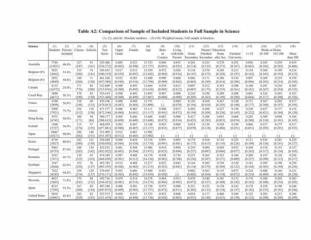
Table A2: Comparison of Sample of Included Students to Full Sample in Science (1), (2), and (4): Absolute numbers. – (5)-(18): Weighted means. Full sample in brackets.

Science (1) (2) (3) (4) (5) (6) (7) (8) (9) (10) (11) (12) (13) (14) (15) (16) (17) (18) Students Percent Classes Schools Test Upper Female Age Born Living Parents’ Education Books at Home Included Score Grade in

Country with both Parents

Some Secondary

Finished Secondary

Some after Sec.

Finished University

11-25 26-100 101-200 Morethan 200

7744 327 93 525.486 0.485 0.523 13.723 0.896 0.835 0.203 0.223 0.270 0.292 0.056 0.245 0.259 0.419Australia [12821] 60.4% [547] [161] [524.272] [0.492] [0.508] [13.727] [0.891] [0.833] [0.214] [0.235] [0.273] [0.267] [0.062] [0.243] [0.265] [0.406]3023 155 74 545.655 0.517 0.515 13.559 0.972 0.926 0.134 0.370 0.245 0.213 0.154 0.360 0.199 0.216Belgium (Fl) [5662] 53.4% [296] [141] [540.319] [0.539] [0.497] [13.642] [0.969] [0.914] [0.147] [0.375] [0.228] [0.197] [0.162] [0.343] [0.193] [0.215]2852 148 71 461.268 0.525 0.583 13.680 0.909 0.860 0.066 0.171 0.386 0.334 0.097 0.269 0.219 0.359Belgium (Fr) [4849] 58.8% [260] [120] [457.588] [0.544] [0.516] [13.794] [0.909] [0.862] [0.065] [0.189] [0.414] [0.296] [0.096] [0.283] [0.214] [0.345]4135 171 84 522.689 0.490 0.493 13.664 0.939 0.815 0.097 0.212 0.355 0.300 0.108 0.291 0.256 0.305Canada [16572] 25.0% [776] [380] [515.076] [0.500] [0.495] [13.634] [0.905] [0.812] [0.087] [0.173] [0.335] [0.361] [0.101] [0.267] [0.254] [0.335]3890 170 85 553.618 0.508 0.492 13.893 0.987 0.908 0.210 0.350 0.209 0.208 0.041 0.326 0.303 0.323Czech Rep. [6671] 58.3% [299] [150] [553.440] [0.500] [0.499] [13.887] [0.988] [0.909] [0.205] [0.363] [0.199] [0.209] [0.044] [0.317] [0.308] [0.326]3350 138 69 476.196 0.488 0.494 13.751 - 0.869 0.156 0.410 0.267 0.120 0.171 0.367 0.202 0.217France [5898] 56.8% [248] [132] [474.053] [0.487] [0.484] [13.808] [-] [0.879] [0.194] [0.410] [0.245] [0.100] [0.177] [0.380] [0.197] [0.195]5998 236 118 471.577 0.486 0.482 13.111 0.940 0.873 0.202 0.208 0.227 0.158 0.228 0.427 0.177 0.116Greece [7921] 75.7% [312] [156] [472.196] [0.484] [0.481] [13.117] [0.941] [0.873] [0.194] [0.208] [0.238] [0.165] [0.222] [0.421] [0.184] [0.120]3975 100 50 509.177 0.505 0.446 13.688 0.883 0.908 0.427 0.288 0.053 0.068 0.285 0.309 0.098 0.104Hong Kong [6745] 58.9% [171] [86] [508.635] [0.499] [0.449] [13.688] [0.873] [0.914] [0.423] [0.283] [0.053] [0.074] [0.280] [0.310] [0.101] [0.105]1448 115 57 468.859 0.503 0.487 13.148 0.955 0.894 0.074 0.120 0.528 0.199 0.066 0.337 0.275 0.317Iceland [3727] 38.9% [274] [155] [477.881] [0.500] [0.487] [13.137] [0.933] [0.877] [0.070] [0.118] [0.496] [0.251] [0.051] [0.295] [0.291] [0.353]10067 296 148 551.909 0.512 0.483 13.902 - - - - - - - - - -Japan [10271] 98.0% [302] [151] [551.507] [0.512] [0.483] [13.902] [-] [-] [-] [-] [-] [-] [-] [-] [-] [-]4710 242 121 550.288 0.504 0.424 13.716 0.991 0.883 0.174 0.418 0.110 0.225 0.111 0.334 0.241 0.229Korea [5827] 80.8% [300] [150] [550.058] [0.504] [0.438] [13.710] [0.991] [0.881] [0.175] [0.415] [0.110] [0.226] [0.109] [0.336] [0.241] [0.227]5903 248 124 452.532 0.481 0.504 13.986 0.919 0.894 0.239 0.094 0.058 0.072 0.269 0.318 0.133 0.157Portugal [6753] 87.4% [283] [142] [452.922] [0.483] [0.504] [13.971] [0.923] [0.894] [0.237] [0.097] [0.060] [0.077] [0.265] [0.317] [0.134] [0.165]3412 130 65 474.249 0.507 0.488 14.170 0.958 0.736 0.253 0.265 0.332 0.104 0.209 0.197 0.126 0.256 Romania [7471] 45.7% [325] [163] [468.850] [0.501] [0.512] [14.124] [0.962] [0.768] [0.256] [0.307] [0.271] [0.089] [0.227] [0.209] [0.113] [0.217]3547 152 76 493.785 0.512 0.488 13.217 0.922 0.843 0.144 0.385 0.350 0.120 0.161 0.305 0.198 0.230Scotland [5666] 62.6% [254] [127] [493.355] [0.506] [0.485] [13.215] [0.923] [0.841] [0.134] [0.375] [0.369] [0.122] [0.164] [0.303] [0.194] [0.236]7822 258 129 576.693 0.503 0.486 13.940 0.921 - 0.002 0.563 0.135 0.073 0.218 0.408 0.146 0.121Singapore [8285] 94.4% [274] [137] [576.171] [0.502] [0.492] [13.939] [0.920] [-] [0.002] [0.564] [0.134] [0.072] [0.219] [0.409] [0.145] [0.120]4023 176 88 542.736 0.479 0.514 14.278 0.964 0.913 0.078 0.340 0.301 0.172 0.176 0.388 0.205 0.203Slovenia [5603] 71.8% [243] [122] [544.433] [0.481] [0.514] [14.274] [0.966] [0.903] [0.072] [0.337] [0.308] [0.182] [0.165] [0.388] [0.216] [0.205]4215 167 82 497.248 0.496 0.501 13.730 0.972 0.906 0.221 0.123 0.128 0.163 0.178 0.328 0.198 0.246Spain [7595] 55.5% [309] [154] [497.075] [0.499] [0.503] [13.757] [0.972] [0.911] [0.205] [0.133] [0.134] [0.157] [0.182] [0.335] [0.191] [0.244]5018 242 82 527.572 0.494 0.515 13.723 0.933 0.808 0.054 0.177 0.406 0.349 0.122 0.283 0.213 0.306United States [10967] 45.8% [529] [183] [521.419] [0.502] [0.498] [13.736] [0.928] [0.803] [0.053] [0.180] [0.423] [0.330] [0.122] [0.290] [0.209] [0.299]

Table A3: Class-Size Effects in Mathematics Using the Log of Class Size Estimates of the coefficient on log class size. Dependent variable: Mathematics test score. Controlling for

grade level and 12 student- and family-background variables. Clustering-robust standard errors in parentheses.

Mathematics (1) (6) (2) (3) (4) (5) (7) Observations (Students) WLSa SFEa SFE-IVa Standard Error Coefficient (α1) Coefficient (α2) Standard Error Coefficient (α3) Standard Error

Australia 9080 65.047† (27.131) 57.838* (20.558) -34.154 (80.165) Belgium (Fl) 3749 41.470† (20.677) 18.317 (21.066) 432.541 (1064.735) Belgium (Fr) 3004 31.913† (14.146) -6.686 (15.348) 5.577 (16.831) Canada 8044 28.760‡ (15.222) 9.730 (9.724) 6.380 (15.896) Czech Rep. 3306 60.125† (28.663) -13.624 (44.899) 112.083 (85.110) France 3938 64.239* (19.817) 46.227† (18.156) -69.019† (34.699) Greece 5528 12.764 (10.504) -19.553 (17.216) -39.576 (25.923) Hong Kong 4385 160.774* (30.692) 130.675* (15.660) -166.939 (230.574) Iceland 1672 1.803 (6.104) -5.906 (7.701) -34.279* (9.862) Japan 10142 -9.948 103.189* (25.927) (10.984) 9.089 (17.932) Korea 5021 -8.799 (6.549) -14.555* (3.796) -49.558‡ (26.756) Portugal 5058 22.301* (5.917) 24.616* (6.534) 36.639† (15.742) Romania 3858 52.319* (15.201) 17.292 (16.937) 40.998 (50.212) Scotland 3219 -122.436 56.201* (16.006) 58.352* (21.027) (210.346) Singapore 8109 138.160* (13.189) 90.533* (11.186) 11.478 (14.974) Slovenia 3644 11.608 (15.028) 0.664 (17.631) 19.375 (28.614) Spain 4313 7.827 (6.212) -1.602 (7.603) 0.231 (22.715) United States 6000 -4.987 (7.203) -0.147 (8.073) -3172.532 (24544.980)

a WLS: Weighted least squares. — SFE: School fixed effects. — SFE-IV: School fixed effects and instrumental variables. — See text for details on the methods of estimation. Significance levels (based on clustering-robust standard errors): * 1 percent. — † 5 percent. — ‡ 10 percent.

Table A4: Class-Size Effects in Science Using the Log of Class Size Estimates of the coefficient on log class size. Dependent variable: Mathematics test score. Controlling for

grade level and 12 student- and family-background variables. Clustering-robust standard errors in parentheses.

Science (1) (2) (3) (4) (5) (6) (7) Observations (Students) WLSa SFEa SFE-IVa Coefficient (α1) Standard Error Coefficient (α2) Standard Error Coefficient (α3) Standard Error

Australia 7744 85.158* (17.393) 32.899‡ (16.936) 9.785 (406.287) Belgium (Fl) 3023 23.438 (15.472) 10.460 (18.407) 18.970 (30.385) Belgium (Fr) 2852 -5.309 (12.658) -24.513‡ (14.217) -11.461 (16.744) Canada 4135 2.941 (6.180) 11.544† (5.617) -27.941 (22.836) Czech Rep. 3890 34.461† (16.999) -44.036† (21.232) -18.738 (24.786) France 3350 10.882 (10.787) -3.695 (12.054) 0.435 (24.238) Greece 5998 14.486* (4.458) -1.532 (4.727) -68.341‡ (36.586)

3975 197.803* (47.984) 125.036* (18.948) -852.418 (1346.080) Iceland 1448 -14.419* (4.736) -11.674 (8.961) -1.427 (17.245) Japan 10067 68.213* (20.747) -13.909 (9.735) 7.860 (22.436) Korea 3.587 4710 7.832† (3.354) (4.641) -33.193 (70.803) Portugal 5903 3.341 (7.016) 1.662 (6.763) -19.768 (22.615) Romania 3412 31.716 (20.701) 25.328 (16.618) 130.564‡ (72.313) Scotland 3547 -11.953 (7.598) -12.151† (5.830) 398.022 (428.458) Singapore 7822 15.419 148.770* (12.921) 100.357* (12.376) (15.326) Slovenia 4023 -11.956 (13.600) 1.232 (13.419) 2.151 (19.099) Spain 4215 8.846 (5.579) 3.780 (6.288) -22.393* (10.136) United States 5018 -1.313 (10.409) 8.300 (8.469) -31.889 (130.550)

Hong Kong

a WLS: Weighted least squares. — SFE: School fixed effects. — SFE-IV: School fixed effects and instrumental variables. — See text for details on the methods of estimation. Significance levels (based on clustering-robust standard errors): * 1 percent. — † 5 percent. — ‡ 10 percent.

Table A5: Class-Size Effects in Mathematics Controlling for Teacher Characteristics Estimates of the coefficient on class size. Dependent variable: Mathematics test score. Controlling for grade level,

12 student- and family-background variables, and the 6 teacher-background variables mentioned below.

Mathematics (1) (13) (2) (3) (4) (5) (6) (7) (8) (9) (10) (11) (12) (14) (15) (16) (17) (18) (19) (20) (21) (22) (23) (24)WLSa Teacher’s Teacher’s Educ. SFEa Teacher’s Educ. SFE-IVa Teacher’s Teacher’s Educ.

Coeff. (α1) Std. Error Sexb Age Exp. Sec. BA MA Coeff. (α2) Std. Error Sexb Age Exp. Sec. BA MA Coeff. (α3) Std. Error Sexb Age Exp. Sec. BA MA

Australia 4.192* (0.724) +† 4.257* (0.647) -1.625 (3.655) Belgium (Fl) 1.118 2.243† (0.110) −* (1.199) −† 4.823 (3.608) −† Belgium (Fr) 1.693† (0.670) +‡ −* +* -0.073 (0.654) +* −* +* -0.617 (0.921) +* −* +* Canada 0.925 (0.819) 0.152 (0.426) +† +† 0.411 (0.605) +† +† Czech Rep. 2.235 (1.375) -0.380 (1.762) −† +‡ 2.871 (2.020) −† +†

France +* +* 2.440* (0.825) +* +* +* 1.452† (0.741) +* +* +* -2.524‡ (1.308) +*

Greece 0.220 (0.445) +* -0.960 (0.710) +‡ -1.552 (1.055) Hong Kong 5.254* (1.117) −‡ 4.360* (0.529) −* -7.698 (10.590) Iceland 0.033 (0.498) +† −‡ -0.246 (0.576) +† −* -2.285* (0.661) +† +† −* Japan 3.801* (0.792) −* -0.317 (0.356) −* +* -0.105 (0.419) −* +*

Korea -0.134‡ (0.074) +* +* -0.157* (0.043) +* +* -0.909 (0.758) +‡ Portugal 0.778* (0.268) +‡ 0.781* (0.223) 1.610‡ (0.729) Romania (0.599) 1.012 2.217* (0.580) +* 0.541 −† +† +* +† (1.890) −† +† +* +‡ Scotland 2.586* (0.657) +† +† 3.023* (0.903) + -2.815 (6.074) +‡ Singapore − 4.743* (0.472) 3.174* (0.422) ‡ 0.578 (0.501)

Slovenia 0.522 (0.663) -0.312 (0.677) +† 0.262 (1.392) +† Spain 0.187 (0.167) -0.016 (0.174) +* +* +* -0.758 (0.898) +* +‡ United States -0.094 (0.111) +‡ 0.005 (0.128) 18.007 (68.053)

Teacher’s

a WLS: Weighted least squares. — SFE: School fixed effects. — SFE-IV: School fixed effects and instrumental variables. — See text for details on the methods of estimation. – b Dummy variable with female = 1 and male = 0. Significance levels (based on clustering-robust standard errors): * 1 percent. — † 5 percent. — ‡ 10 percent.

Table A6: Class-Size Effects in Science Controlling for Teacher Characteristics Estimates of the coefficient on class size. Dependent variable: Mathematics test score. Controlling for grade level,

12 student- and family-background variables, and the 6 teacher-background variables mentioned below.

Science (1) (2) (3) (4) (5) (6) (7) (8) (9) (10) (11) (12) (13) (14) (15) (16) (17) (18) (19) (20) (21) (22) (23) (24)WLSa Teacher’s Teacher’s Educ. SFEa Teacher’s Teacher’s Educ. SFE-IVa Teacher’s Teacher’s Educ.

Coeff. (α1) Std. Error Sexb Age Exp. Sec. BA MA Coeff. (α2) Std. Error Sexb Age Exp. Sec. BA MA Coeff. (α3) Std. Error Sexb Age Exp. Sec. MA

Australia 3.564* (0.660) 1.506† (0.682) -4.089 (10.994) Belgium (Fl) 1.475‡ (0.874) 0.357 (1.016) −* 0.992 (1.415) −* Belgium (Fr) -0.528 (0.627) −† +‡ -1.132 (0.683) +† −* +† -0.659 (1.181) −* +† Canada + 0.074 (0.010) −† −* −* 0.051 (0.082) +* −* −† -1.255 (1.069) ‡ −* −* Czech Rep. 0 + 1.251‡ (0.723) -2.03 † (0.810) † -1.158 (0.986) +‡

France 0.600 (0.490) 0.075 (0.475) −† +* 0.138 (0.876) −† −* Greece 0.290* (0.086) +* +* 0.093 (0.068) +‡ -2.620‡ (1.353) Hong Kong 5.500* (1.270) 3.420 (0.649) +† −† +† -9.585 (8.119) +‡ Iceland -1.010* (0.313) +† +† -1.036† (0.443) +* +* +* -1.263 (0.987) +* +* +* Japan 2.567* (0.666) -0.447 (0.297) -0.285 (0.404)

Korea 0.194 (0.118) −* −* 0.042 (0.104) −† -0.738 (1.248) −† 0.170 (0.296) +‡ 0.094 (0.291) +* -0.376 (0.557) +†

Romania 0.924 (0.841) −* +† +† +‡ 0.646 (0.659) +† +* 3.075 (2.327) +‡ +* Scotland 8 (0.282) − -0.735† (0.323) −† +† -0.55 † † −* −* 35.442 (105.381) Singapore (0.487) 4.959* (0.482) +* +‡ +‡ 3.326* (0.427) +† 0.440 +*

Slovenia -0.388 (0.584) * +‡ +* +* -0.522 (0.583) −† +* +* + -0.161 (0.943) −† +* +* +* Spain 0.116 (0.157) +‡ 0.128 (0.181) +‡ +† −* -0.693* (0.265) +‡ −* United States 0.021 (0.179) 0.205 (0.151) −‡ -0.770 (2.763)

BA

Portugal

a WLS: Weighted least squares. — SFE: School fixed effects. — SFE-IV: School fixed effects and instrumental variables. — See text for details on the methods of estimation. – b Dummy variable with female = 1 and male = 0. Significance levels (based on clustering-robust standard errors): * 1 percent. — † 5 percent. — ‡ 10 percent.

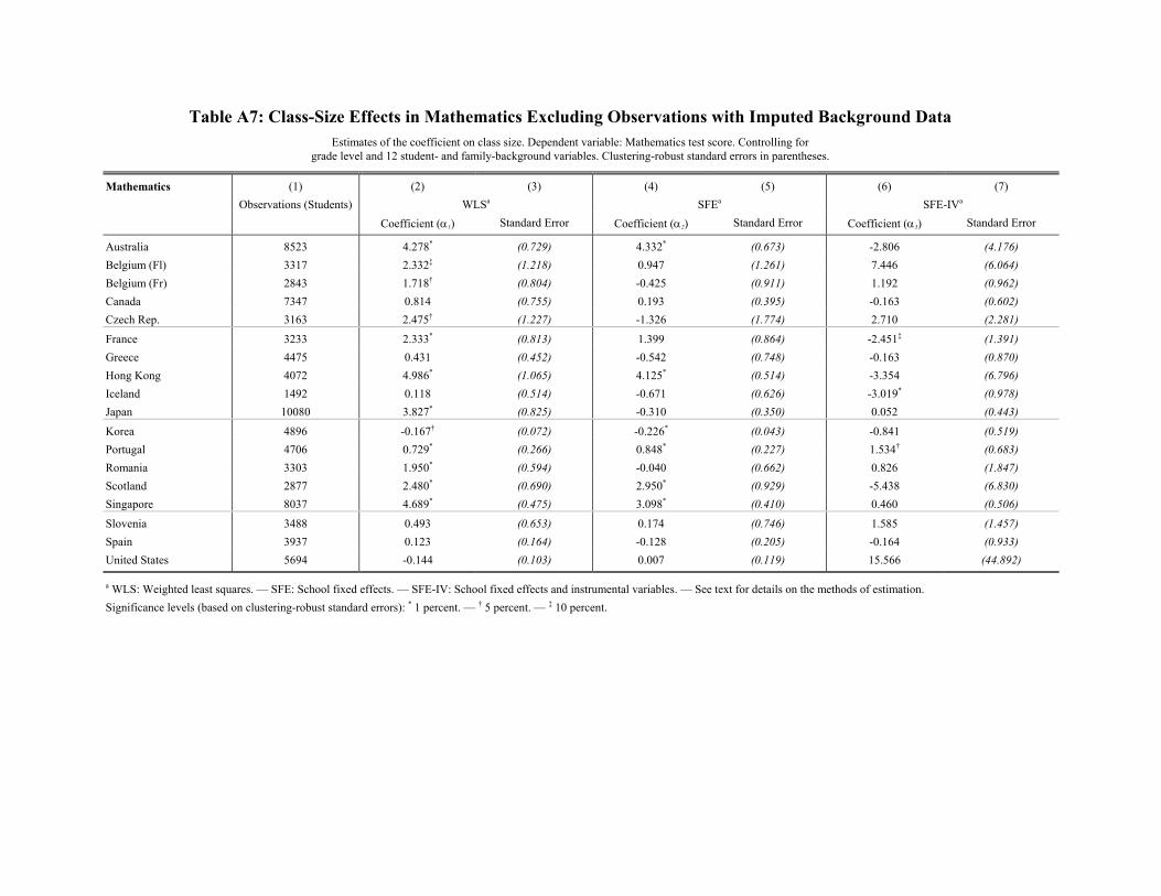
Table A7: Class-Size Effects in Mathematics Excluding Observations with Imputed Background Data Estimates of the coefficient on class size. Dependent variable: Mathematics test score. Controlling for

grade level and 12 student- and family-background variables. Clustering-robust standard errors in parentheses.

Mathematics (1) (2) (3) (4) (5) (6) (7) Observations (Students) WLSa SFEa SFE-IVa Coefficient (α1) Standard Error Coefficient (α2) Standard Error Coefficient (α3) Standard Error

Australia 8523 4.278* (0.729) 4.332* (0.673) -2.806 (4.176) Belgium (Fl) 3317 2.332‡ (1.218) 0.947 (1.261) 7.446 (6.064) Belgium (Fr) 2843 1.718† (0.804) -0.425 (0.911) 1.192 (0.962) Canada 7347 0.814 (0.755) 0.193 (0.395) -0.163 (0.602) Czech Rep. 3163 2.475† (1.227) -1.326 (1.774) 2.710 (2.281)

France 3233 2.333* (0.813) 1.399 (0.864) -2.451‡ (1.391) Greece 4475 0.431 (0.452) -0.542 (0.748) -0.163 (0.870) Hong Kong 4072 4.986* (1.065) 4.125* (0.514) -3.354 (6.796) Iceland 1492 0.118 (0.514) -0.671 (0.626) -3.019* (0.978) Japan 10080 3.827* (0.825) -0.310 (0.350) 0.052 (0.443)

Korea 4896 -0.167† (0.072) -0.226* (0.043) -0.841 (0.519) Portugal 4706 0.729* (0.266) 0.848* (0.227) 1.534† (0.683) Romania 3303 1.950* (0.594) -0.040 (0.662) 0.826 (1.847) Scotland 2877 2.480* (0.690) 2.950* (0.929) -5.438 (6.830) Singapore 8037 4.689* (0.475) 3.098* (0.410) 0.460 (0.506)

Slovenia 3488 0.493 (0.653) 0.174 (0.746) 1.585 (1.457) Spain 3937 0.123 (0.164) -0.128 (0.205) -0.164 (0.933) United States 5694 -0.144 (0.103) 0.007 (0.119) 15.566 (44.892)

a WLS: Weighted least squares. — SFE: School fixed effects. — SFE-IV: School fixed effects and instrumental variables. — See text for details on the methods of estimation. Significance levels (based on clustering-robust standard errors): * 1 percent. — † 5 percent. — ‡ 10 percent.

Table A8: Class-Size Effects in Science Excluding Observations with Imputed Background Data Estimates of the coefficient on class size. Dependent variable: Science test score. Controlling for

grade level and 12 student- and family-background variables. Clustering-robust standard errors in parentheses.

Science (1) (2) (3) (4) (5) (6) (7) Observations (Students) WLSa SFEa SFE-IVa Coefficient (α1) Standard Error Coefficient (α2) Standard Error Coefficient (α3) Standard Error

Australia 7340 3.682* (0.603) 1.628† (0.682) -3.275 (9.658) Belgium (Fl) 2692 1.502‡ (0.846) 0.246 (0.970) 0.446 (1.426) Belgium (Fr) 2708 -0.333 (0.608) -1.384‡ (0.787) -0.057 (1.065) Canada 3828 0.046 (0.086) 0.0192† (0.092) -0.636 (1.112) Czech Rep. 3730 1.552† (0.707) -1.666‡ (0.920) -1.044 (0.943)

France 2786 0.758 (0.493) 0.410 (0.554) 0.654 (0.833) Greece 4876 0.329† (0.138) 0.069 (0.057) -2.208 (1.397) Hong Kong 3609 5.327* (1.259) 3.590* (0.680) -12.858 (13.992) Iceland 1295 -1.022* (0.369) -0.446 (0.754) -1.269 (1.488) Japan 10005 2.606* (0.674) -0.433 (0.310) -0.189 (0.453)

Korea 4588 0.216 (0.113) 0.111 (0.098) -0.769 (1.277) Portugal 5501 0.186 (0.300) 0.113 (0.290) -0.018 (0.551) Romania 2999 1.269 (0.853) 0.375 (0.673) 3.588 (2.314) Scotland 3162 -0.769† (0.360) -0.647† (0.305) 25.551 (33.469) Singapore 7748 5.017* (0.479) 3.475* (0.453) 0.545 (0.515)

Slovenia 3866 -0.357 (0.620) 0.388 (0.563) 0.568 (0.867) Spain 3839 0.167 (0.165) 0.099 (0.203) -0.813* (0.271) United States 4750 0.034 (0.172) 0.180 (0.142) -1.768 (3.049)

a WLS: Weighted least squares. — SFE: School fixed effects. — SFE-IV: School fixed effects and instrumental variables. — See text for details on the methods of estimation. Significance levels (based on clustering-robust standard errors): * 1 percent. — † 5 percent. — ‡ 10 percent.