classical and quantum strategies for bit commitment...
TRANSCRIPT

Classical and quantum strategies for bitcommitment schemes in the two-prover model
Jean-Raymond Simard
School of Computer Science
McGill University
Montreal, Quebec
February 2007
A thesis submitted to McGill University in partial fulfilment of the requirements of the
degree of Master of Science
c© Jean-Raymond Simard MMVII

Remerciements
Je tiens a remercier Claude Crepeau, mon superviseur, pour son soutien, sa confiance et tout
le temps qu’il m’a consacre. Merci a Louis Salvail et Alain Tapp, sans qui cette recherche
n’aurait probablement pas avancee si vite. Un gros merci a Simon Pierre Desrosiers,
pour l’incroyable travail de correction qu’il a fait sur ce travail, ainsi que pour toutes les
savoureuses discussions que nous avons eues. Merci a tous ceux qui m’ont appuye jusqu’ici,
specialement ma famille, mes amis et professeurs. Finalement, merci a ma copine, Audrey
Desautels, pour tout l’encouragement, les petits mots et tous les beaux moments passes
avec moi a essayer de comprendre ce que je racontais.
Merci aussi au Conseil de recherches en sciences naturelles et en genie du Canada, et
aux Fonds quebecois de la recherche sur la nature et les technologies, pour m’avoir soutenu
financierement durant ces deux annees.
2

Abstract
We show that the long-standing assumption of “no-communication” between the provers
of the two-prover model is not sufficiently precise to guarantee the security of a bit com-
mitment scheme against malicious adversaries. Indeed, we show how a simple correlated
random variable, which does not allow to communicate, can be used to cheat a simpli-
fied version (sBGKW) of the bit commitment scheme of Ben-Or, Goldwasser, Kilian, and
Wigderson [BGKW88]. Instead we propose a stronger notion of separation between the
two provers which takes into account correlated computations. To emphasize the risk that
entanglement still represents for the security of a commitment scheme despite the stronger
notion of separation, we present two variations of the sBGKW scheme that can be cheated
by quantum provers with probability (almost) one. A complete proof of security against
quantum adversaries is then given for the sBGKW scheme. By reduction we also obtain
the security of the original BGKW scheme against quantum provers. For the unfamiliar
reader, basic notions of quantum processing are provided to facilitate the understanding of
the proofs presented.
3

Resume
Dans ce memoire, nous montrerons que l’hypothese traditionnelle d’impossibilite de commu-
nication faite dans le modele a deux proveurs n’est pas suffisamment precise pour garantir
la securite d’un protocole de mise en gage contre des prouveurs malhonnetes. Nous mon-
trerons comment une variable aleatoire correlee, ne permettant pas de communiquer, peut
etre utilisee pour tricher une version simplifiee (sBGKW) du protocole de mise en gage de
Ben-Or, Goldwasser, Kilian, and Wigderson [BGKW88]. Pour resoudre ce probleme, nous
proposerons une notion de separation entre les deux prouveurs beaucoup plus forte que
l’hypothese traditionnelle. Afin de mettre en evidence le risque que constitue l’intrication
pour la securite d’un protocole de mise en gage, nous presenterons deux variations du
protocole sBGKW qui peuvent etre triche par des prouveurs quantiques avec probabilite
(presque) un. Une demonstration detaillee de la securite quantique du protocole sBGKW
sera ensuite donnee. La securite quantique du protocole original de BGKW sera ensuite
obtenue par reduction. Un bref apercu des notions de bases d’informatique quantique sera
propose en introduction pour faciliter la comprehension des demonstrations presentees dans
ce memoire.
4
Contents
Remerciements 2
Abstract 3
Resume 4
Contents 5
Introduction 8
The two-prover model . . . . . . . . . . . . . . . . . . . . . . . . . . . . . . . . . 8
Bit commitment scheme . . . . . . . . . . . . . . . . . . . . . . . . . . . . . . . . 12
Related Works . . . . . . . . . . . . . . . . . . . . . . . . . . . . . . . . . . . . . 15
Organization of the thesis and contributions . . . . . . . . . . . . . . . . . . . . . 16
1 Preliminaries and background 18
1.1 Basic notions of quantum mechanics . . . . . . . . . . . . . . . . . . . . . . 18
1.1.1 Hilbert space, the bra-ket notation and the qubit . . . . . . . . . . . 18
1.1.2 The trace function . . . . . . . . . . . . . . . . . . . . . . . . . . . . 21
1.1.3 Tensor product . . . . . . . . . . . . . . . . . . . . . . . . . . . . . . 22
1.1.4 Important matrix properties . . . . . . . . . . . . . . . . . . . . . . . 23
1.1.5 Measurements . . . . . . . . . . . . . . . . . . . . . . . . . . . . . . 24
1.1.6 Entanglement . . . . . . . . . . . . . . . . . . . . . . . . . . . . . . . 27
1.2 Security definitions . . . . . . . . . . . . . . . . . . . . . . . . . . . . . . . . 28
5
1.3 Non-local games . . . . . . . . . . . . . . . . . . . . . . . . . . . . . . . . . 32
2 Bit commitment in the two-prover model 36
2.1 The original scheme . . . . . . . . . . . . . . . . . . . . . . . . . . . . . . . 36
2.2 A simpler version . . . . . . . . . . . . . . . . . . . . . . . . . . . . . . . . . 38
2.3 Cheating sBGKW with a NL-box . . . . . . . . . . . . . . . . . . . . . . . . 40
2.3.1 The NL-box that breaks the original BGKW scheme . . . . . . . . . 41
2.4 Defining isolation . . . . . . . . . . . . . . . . . . . . . . . . . . . . . . . . . 42
2.5 Fixing the proof of Theorem 2.3 . . . . . . . . . . . . . . . . . . . . . . . . 52
3 Intermediate schemes towards quantum secure bit commitment 54
3.1 A weaker acceptance criteria: the wBGKW scheme . . . . . . . . . . . . . . 54
3.2 The Magic Square . . . . . . . . . . . . . . . . . . . . . . . . . . . . . . . . 56
3.2.1 The game . . . . . . . . . . . . . . . . . . . . . . . . . . . . . . . . . 56
3.2.2 Magic Square bit commitment . . . . . . . . . . . . . . . . . . . . . 57
4 Quantum secure bit commitment in the two-prover model 61
4.1 The scheme . . . . . . . . . . . . . . . . . . . . . . . . . . . . . . . . . . . . 61
4.2 mBGKW is secure against quantum adversaries . . . . . . . . . . . . . . . . 62
4.3 Reduction to the original BGKW scheme . . . . . . . . . . . . . . . . . . . . 68
Conclusion and open problems 70
A Classical and quantum optimal implementation of the NL-box and the
Magic Square game 72
A.1 The CHSH game . . . . . . . . . . . . . . . . . . . . . . . . . . . . . . . . . 73
A.1.1 Optimal classical strategy for the CHSH game . . . . . . . . . . . . 73
A.1.2 Optimal quantum strategy for the CHSH game . . . . . . . . . . . . 75
A.2 The Magic Square game . . . . . . . . . . . . . . . . . . . . . . . . . . . . . 80
A.2.1 Optimal strategy for classical players . . . . . . . . . . . . . . . . . . 81
A.2.2 Quantum winning strategy . . . . . . . . . . . . . . . . . . . . . . . 82
6

Bibliography 84
7

Introduction
The two-prover model
The two-prover model, and its generalized version with k provers, was first introduced by
Ben-Or, Goldwasser, Kilian, and Wigderson [BGKW88] to prove that all NP languages
have a two-prover perfect zero-knowledge interactive proof-system, without having to make
intractability assumptions, such as the existence of one-way functions used in [GMW86]
which is necessary to prove a similar result in the one-prover model. At the time, their
result was of great importance since such a general statement was known to be impossible
in the one-prover model, unless the polynomial-time hierarchy collapsed [For87].
Loosely speaking, an interactive proof-system (IPS) consists of an all powerful prover
who attempts to convince a probabilistic polynomial-time bounded verifier of the truth of a
proposition [GMR85]. It is termed perfect zero-knowledge if there exists a prover such that
for any verifier there exists a stand-alone polynomial-time simulator, not interacting with
anybody, whose output has the same probability distribution as the output produced by
the verifier after interacting with the prover. That is, whatever can be efficiently extracted
from the interaction with the prover when input a proposition, can also be efficiently ex-
tracted from the proposition itself.
Using the formalism of IPS, the setting of the two-prover model consists of two provers,
Peggy and Paula, sometime taken to be computationally unbounded, who jointly agree on
a strategy to convince the verifier, Vic, of the truth of an assertion under the constraint
8

that Peggy and Paula cannot communicate with each other once the interaction with Vic
has started. This no-communication limitation is the key point which allows Vic to decide
whether he should accept or not the proposition. We stress that the two-prover model is
defined as a synchronous model. This means that, although no prover can get the content
of the conversations between Vic and the other prover, a prover can see that messages are
exchanged between the other two participants. The model may be depicted as in Figure 1.
Vic
Paula
Peggy
separation
interaction
interaction
Figure 1: The two-prover model
The authors of [BGKW88] give a particularly enlightening example to illustrate the
power of the two-prover model, as they note:
“The main novelty of our model is that the verifier can “check” its interactions
with the provers “against each other”. One may think of this as the process of
checking the alibi of two suspects of a crime (who have worked long and hard to
prepare a joint alibi), where the suspects are the provers and the verifier is the
interrogator. The interrogator’s conviction that the alibi is valid stems from his
conviction that once the interrogation starts, the suspects can not talk to each
other as they are kept in separate rooms, and since they can not anticipate the
randomized questions he may ask them, he can trust his findings.”
From then on, the two-prover model has been extensively studied and numerous fun-
damental results in the theory of computation were found. A few years after BGKW’s
9
results, Babai, Fortnow and Lund [BFL90] used the same model to prove that every lan-
guage is in NEXP (the non-deterministic exponential-time complexity class) if and only
if it has a many-rounds perfect zero-knowledge two-prover IPS. This result was in sharp
contrast to what was previously expected since Fortnow, Rompel, and Sipser [FRS94] had
shown that relative to some oracle, even the class coNP did not have a multi-prover IPS.
Several refinements of [BFL90]’s result were then made [CCL90, Fei91, LS91], until Feige
and Lovasz [FL92] proved that a language is in NEXP if and only if it has a two-prover
one-round interactive proof system with perfect completeness (if a word is in the language
than the verifier always accepts) and exponentially small soundness error (if a word is not
in the language than the probability of accepting it is exponentially small). This last result
closed the subject on which complexity class may be achieved in the two-prover model with
classical provers.
In the quantum case, the situation is filled with fuzziness. To this day, it is still not
known which complexity class may be achieved with an IPS in a two-quantum-prover against
a quantum-verifier situation. One promising way to tackle the problem is by first consid-
ering one-round IPS with a classical verifier. This means that the interaction between the
verifier and a prover is limited to one round: a query and an answer. Notice that Feige and
Lovasz [FL92] used the classical flavor of this setting to prove their result. This special case
of the two-prover model is particularly interesting to us as it corresponds to the setting of
the so-called non-local games (see Section 1.3). Naturally, a good understanding of such
games will help determine what happens when the provers share entanglement. Recently
Cleve, Høyer, Toner and Watrous investigated this subject [CHTW04] from the point of
view of non-locality and made clear connections with multi-prover IPS. They gave various
examples of one-round multi-prover IPS which are classically sound but where entangle-
ment seriously affects the soundness of the proof system. They also looked at the amount of
entanglement required by optimal and nearly optimal quantum strategies for these games.
More specifically, they showed why the known protocol which equates NEXP to the two-
prover IPS breaks down if the provers can share entanglement, unless EXP=NEXP.
10
We claimed in the previous paragraph that it is not known which class may be achieved
in a two-quantum-prover against a quantum-verifier situation. This is not completely true.
For a restricted case, when the provers share only a polynomial number of qubits, it has
been demonstrated by Kobayashi and Matsumoto [KM03] that the class of languages ac-
cepted by a two-prover IPS is included in NEXP. Whether the two classes are equal is
still an open problem. Recently, Gavinsky [Gav06] gave a partial converse to the result
of [KM03] using a new approach for bounding entanglement, and the parallel repetition
theorem of [Raz95] for improving the soundness of a known classical two-prover IPS which
accepts NEXP. He showed that in order to cheat, the provers require a number of entangled
qubits asymptotically close to the number of parallel repetitions. Thus, by bounding the
amount of shared qubits by some a priori fixed polynomial in the input length1, enough
repetitions can be introduced to make any cheating impossible. Formally,
Theorem [Gav06]: Let MIP ∗poly(n) be the model of two-prover IPS when the provers
are allowed to share any entangled state over poly(n) qubits, where n is the input length of
the problem. Then MIP ∗poly(n) can accept a language L if and only if L ∈ NEXP.
In other words, the power of MIP ∗poly(n) and that of the classical two-prover IPS (equiv-
alent to NEXP) are the same. However, more general results with respect to MIP ∗∞ and
NEXP are not known yet. The problems of integrating the zero-knowledge aspect in a
two-prover IPS with quantum players and which complexity class may be reached are even
less known.1In [KM03] the provers are allowed a fixed number of shared qubits per protocol. However, in [Gav06]
the provers are allowed a fixed number of shared qubits for the whole model. This is what makes [Gav06]’s
converse only partial, since in [KM03] the provers have more freedom.
11

Bit commitment scheme
The cryptographic primitive known as a commitment scheme (often prefixed with bit when
the committed word is a bit) has been one of the major building blocks of cryptography
from its advent in the early 80’s. Although it seems fair to attribute the concept to M.
Blum [Blu82], the terminology of commitments, influenced by the legal vocabulary, first
appeared in the contract signing protocol of S. Even [Eve82]. Commitment lies at the heart
of important complex cryptographic applications such as coin tossing [Blu82], two-party
computation [Kil88] and zero-knowledge proofs [GMW91, BCC88].
The general idea and security of bit commitment is often best explained from this sim-
ple example: suppose Alice wants to commit to a certain secret bit value b to Bob without
him learning this value before she decides it. To do so, she writes b down on a piece
of paper, puts the paper in a box which she locks with a key; she then gives the locked
box to Bob (who does not have the ability to pick it). This first stage in the protocol is
called committing. Whenever Alice consider that Bob is ready to learn her bit, she sends to
him the key, he opens the box and learns the value of b. This second stage is called unveiling.
As illustrated in the example, there are two essential aspects to the security of a bit
commitment scheme:
1. Once Alice commits to her bit, she cannot change her mind and reveal to Bob a
different bit value. This is known as the binding property of the commitment.
2. Until unveiling starts, Bob cannot learn to which value Alice committed. This is
known as the concealing property of the commitment.
Of course, these security characteristics naturally extend to the more general form of com-
mitment scheme known as string commitment.
It has been known for long that unconditionally secure classical bit commitment is
12

impossible2. So to achieve some security properties, extra assumptions need to be made.
For instance, computational assumptions can be imposed on the binding or concealing
properties. Under such restrictions, commitments come in two dual flavors: binding but
computationally concealing and concealing but computationally binding. The first type
may be achieved from any one-way function [Nao91, HILL98]. Those of the second type
may be achieved from any one-way permutation [NOVY93] or any collision-free hash func-
tion [HM96]. The problem of achieving commitments of the second type using only one-way
functions is still open.
When Bennett and Brassard [BB84] brought back to life the idea of Wiesner [Wie70]
to use quantum physics to achieve cryptographic tasks, a lot of hopes and efforts were
put by cryptographers to revitalize the security of commitment schemes without any extra
assumption. The first form of quantum bit commitment came implicitly with the BB84
coin-flipping protocol [BB84]. However, problems relating to the physical control of the
quantum system made it easy to cheat for the receiver in practice. Bennett and Brassard
also pointed out that it was possible, in theory, for the sender to cheat the binding property
of the commitment. To solve these two problems, Brassard, Crepeau, Josza and Langlois
[BCJL93] presented a new protocol, which was in fact an extension of the protocol found
in [BC90], along with a “proof” of its unconditional security against quantum adversaries.
For a while, most people were convinced that quantum bit commitment could be performed
securely.
Unfortunately, rarely do nice things happen without any surprises. Doubts on the se-
curity of the BCJL’s protocol against the sender settled in when, a couple of years after
their result, Mayers found a subtle flaw in the proof and gave a specific attack to the pro-2The intuition behind the proof is simple. Unconditional security requires an information theoretic
argument. Let C be the random variable representing the commitment. To satisfy the binding property,
C must hold a lot of information about the committed bit. However, to satisfy the concealing property, C
must not hold any information on the committed bit. It is easy to see that C cannot satisfy both properties
at the same time.
13

tocol. Mayers and the BCJL team then engaged in a battle of attacks and corrections
of the protocol for about a year, until Mayers finally draw the final strike with its gen-
eral impossibility theorem for quantum bit commitment [May96a, May96b]. We note that
a similar result was, around the same time, independently achieved by Lo and Chau [LC97].
In their ’98 paper [BCMS98], Brassard et al. nicely stated the disappointment:
“[...] In 1993 a protocol for quantum bit commitment, henceforth referred to as
BCJL, was thought to be “provably secure”. Because of quantum bit commit-
ment, the future of quantum cryptography was very bright, with new applications
such as the identification protocol of Crepeau and Salvail [CS95] coming up reg-
ularly. The trouble began in October 1995 when Mayers found a subtle flaw in
the BCJL protocol. [...] After BCJL was shown not secure, the spontaneous at-
titude was to try alternative quantum bit commitment protocols by making some
clever use of measurements and classical communication. However, all of these
protocols were found not secure against Mayers’ attack!”
Nevertheless, the fate of quantum bit commitment is not sealed definitely. The general
impossibility theorem of Mayers and Lo-Chau does not apply in all communication models.
Indeed, the possibility of unconditionally secure (quantum) bit commitment has already
been demonstrated in various models different from the standard noiseless communication
model with two players, namely:
• the noisy communication model [CK88, Cre97, DFMS04, DKS99, CMW04],
• the multi-party computations model [BGW88, CCD88],
• the multi-prover model under some relativistic time constraint [Ken05, Ken99],
• the (quantum) memory-bounded model [CCM98, DFSS05],
• the multi-prover model under some physical separation constraints [BGKW88].
The fifth scenario, where we consider the case of two provers, is our main focus here.
In [BGKW88], the authors introduced a bit commitment scheme for which they gave an
14

unconditional security proof against classical adversaries. Here we wish to provide a similar
proof against adversaries that have full access to quantum resources.
Related Works
The starting point of this research is definitely the bit commitment scheme introduced by
Ben-Or, Goldwasser, Kilian and Wigderson in [BGKW88] to provide a sufficient toolbox
for their two-prover interactive proof-system to be perfect zero-knowledge. The classical
security of their scheme is proven in [BGKW88].
The security of BGKW’s scheme against quantum adversaries has been considered in
the work of Brassard, Crepeau, Mayers and Salvail [BCMS98]. They showed that if such
a bit commitment is used as a building block in the Quantum Oblivious Transfer protocol
of [CK88] then the security of the commitment scheme is not sufficient to guarantee the
security of the resulting QOT if the two provers can get back together at the end of the pro-
tocol. This result is in accordance with Mayers’ suggestion [May97] that his version of the
no-go theorem should also apply to commitment schemes based on temporary relativistic
signaling constraints. However they did not address directly the question whether BGKW’s
bit commitment scheme is itself secure against quantum adversaries while the provers are
not allowed to get back together. In the current work, we consider precisely this situation.
In a closely related work, Kent [Ken05] showed how impossibility of communication,
implemented through relativistic assumptions, may be used to obtain a bit commitment
scheme similar to BGKW’s. Although the model he considered is essentially classical, he
also discussed how his scheme behaves in a quantum setting. Kent proves the classical
security of his scheme, but he remained elusive about its quantum security. Still, he proves
the security of one round of his protocol (see [Ken05], Lemma 3, p. 329) against quantum
adversaries, which is more or less the same as our Lemma 4.1. However, the proof he gave
is erroneous in its last inequality and is not as tight as he claims. Lemma 4.1 can be viewed
15
as a notable clarification, and a fix for his proof. Among the differences with the scheme
we present in this work, we note that his bit commitment scheme needs to be constantly
updated (there is always new commitments made) to avoid cheating the first commitment
made, whereas in ours we only need to maintain the physical separation assumption between
the two provers for the commitment to remain secure. This particularity of his protocol
translates in a constant blowup of the communication complexity proportional to the time
we want to sustain the commitment, since a permanent flow of communications needs to
be set between the two parties.
Another related line of research by Cleve, Høyer, Toner and Watrous [CHTW04], is
one of the main inspiration of the current research as briefly discussed in the introduction.
They have established nice relations between non-locality games and the two-prover model.
They developed methods for establishing limits on the nonlocal behavior of such games to
characterize how the soundness of two-prover IPS is affected. They also investigated the
amount of entanglement required by (nearly) optimal quantum strategies to achieve these
limits. However they did not consider how the zero-knowledge aspect of the studied IPS is
affected by quantum adversaries.
Organization of the thesis and contributions
The remainder of the present document is organized as follows. Chapter 1 presents an
overview of the basic notions of quantum mechanics needed to understand this work. We
review the security definitions of a bit commitment scheme against classical and quantum
adversaries, and briefly discuss a new binding definition recently introduced by Damgaard,
Fehr, Salvail and Schaffner [DFSS06]. We also present some definitions and theorems that
relate to non-local games. Chapter 2 introduces the original two-prover bit commitments of
[BGKW88] and exposes the various problems (weakness) of the model’s assumption “that
the two provers are not allowed to talk to each other”; this chapter concludes with a re-
finement of BGKW’s original assumption. In Chapter 3 we present two bit commitment
16
schemes in the two-prover model and show how entanglement-based strategies can be used
to cheat each of them. Finally, Chapter 4 presents a variation of the bit commitment of
Section 2.2 and prove its security against quantum adversaries. We obtain by reduction
that the original BGKW’ scheme is also secure against quantum adversaries. We conclude
with some open problems. Appendix A treats of the classical and quantum optimal strate-
gies to implement what we call the “NL-box” (see Section 2.3) and the Magic Square game
(see Section3.2).
Parts of Chapter 2 (specifically sections 2.2, 2.3, and 2.4), Chapter 3, and Chapter
4 are all original contributions in which the author of the present work has intensively
participated, in collaboration with Claude Crepeau, Louis Salvail, and Alain Tapp.
17
Chapter 1
Preliminaries and background
This chapter introduces the basic definitions and results that relate to quantum mechanics
and information processing, to the security of bit commitment, and to the so-called non-
local games. In no circumstances is this chapter meant to be a comprehensive introduction
to the three subjects. Its sole purpose is to provide the reader with the specific tools
required for the understanding of the present work. The interested reader is invited to
consult [NC00] and [Bro04] for more information on these areas.
1.1 Basic notions of quantum mechanics
1.1.1 Hilbert space, the bra-ket notation and the qubit
The basic objects of linear algebra are vector spaces, themselves composed of elements
called vectors. For instance, Cn is the space of all n-tuples (a.k.a. vectors) of complex
numbers (v1, . . . , vn). A useful representation for vectors is the column matrix notationv1...
vn
. (1.1)
18
Let ϕ be such an object. In linear algebra, the standard notation to indicate that ϕ is a
vector is to write it toped with an arrow pointing in the right direction
~ϕ.
The type of vectors used in quantum mechanics are those of norm one. However, for
historical reasons physicists have decided not to use the previous notation. Instead, in
quantum mechanics the standard way to indicate that the object ϕ is a vector of norm one
is to label it as
|ϕ〉.
The entire object |ϕ〉 is sometimes called a ket, and it is part of a set of similar labels known
as the Dirac notation. In the same manner, we define the bra as the dual vector of |ϕ〉
〈ϕ| :=[v1 . . . vn
],
where vi is the complex conjugate of vi. One can see that a bra is simply a ket conjugated
and transposed. These two transformations are usually represented using a dagger sign †
〈ϕ| def= |ϕ〉T def= |ϕ〉†.
Most vector spaces are not interesting unless an inner product function is defined on
that space. For the vector space Cn, the inner product between vectors |ψ〉 = [u1, . . . , un]T
and |ϕ〉 = [v1, . . . , vn]T is defined as
〈ψ|ϕ〉 :=[u1 . . . un
]·
v1...
vn
=∑
i
uivi.
Similarly, the outer product between vectors |ψ〉 and |ϕ〉 is defined as
|ψ〉〈ϕ| :=
u1
...
un
· [ v1 . . . vn
].
In quantum mechanics’ terminology, the complex vector space of dimension d equipped
with such an inner product is usually referred to as a Hilbert space, denoted Hd. For a
19

finite d, the Hilbert space is exactly the same as the complex inner product space. More-
over, quantum mechanics postulates that, to any isolated physical system we can associate
a Hilbert space, known as the state space. The state of the system is completely described
by a vector of norm one in that Hilbert space, known as the state vector. This first pos-
tulate is particularly important as it makes a connection between the physical world and
the mathematical formalism of quantum mechanics. To avoid any irrelevant description of
a system, from now on we assume that all the vectors in Hd are of norm one.
We know that a vector space of dimension d is spanned by a set of d vectors |ϕ0〉 to
|ϕd−1〉, such that any vector |ϕ〉 in that space can be written as a linear combination of the
vectors in that set, that is,
|ϕ〉 =d−1∑i=0
ai|ϕi〉 where ai ∈ C.
This set of vectors is called a basis of the vector space. It is conventional to define the
computational basis of dimension 2d as the set {|i〉}i∈{0,1}d where
|i〉 =
z0...
z2d−1
s.t. zj =
0 j 6= i
1 j = i.
The simplest quantum mechanical system, and the one with which we will be most
concerned for quantum computation and information, is called the qubit. A qubit lives is
a two-dimensional Hilbert space H2; that is, it has a two-dimensional state space. Using
the computational basis {|0〉, |1〉}, we can express an arbitrary state vector |ϕ〉 ∈ H2 of the
qubit as a superposition
|ϕ〉 = α|0〉+ β|1〉,
where |α|2 + |β|2 = 1. Hence, contrary to the classical bit that can take only values zero
and one, the qubit can take any combinations of those values in H2, and in particular |0〉
and |1〉.
20

1.1.2 The trace function
The trace of an arbitrary matrix A = {aij} is defined to be the sum of its diagonal elements,
Tr(A) :=∑
i
aii. (1.2)
For A,B and C, arbitrary matrices, and z a complex number, the following important
properties hold:
1. Cyclic property of trace
Tr(ABC) = Tr(BCA).
2. Linearity of trace
Tr(A+B) = Tr(A) + Tr(B),
Tr(zA) = zTr(A).
Consider the operator A and a unit vector |ϕ〉, then an extremely useful corollary of the
cyclic property of trace is
Tr(A|ϕ〉〈ϕ|) = 〈ϕ|A|ϕ〉. (1.3)
Let A be of dimension d and |i〉 any orthonormal basis of dimension d. Using (1.3) and
the completeness relation of the basis,∑
i |i〉〈i| = Id, we can give an alternative definition
for the trace function,
Tr(A) = Tr(A · Id) = Tr
(A∑
i
|i〉〈i|
)=
∑i
Tr (A|i〉〈i|)
=∑
i
〈i|A|i〉.
21
1.1.3 Tensor product
The tensor product construction is a crucial element to manipulate a multi-particle system.
Indeed, the fourth postulate of quantum mechanics stipulates that the state space of a
composite system is the tensor product of the state space of the component systems.
Let us first give a concrete idea of the tensor product with a matrix representation. Let
A be an m × n matrix, and B a p × q matrix. The tensor product of A with B is defined
as the nq ×mp matrix
A⊗B :=
a11B a12B . . . a1nB
a21B a22B . . . a2nB...
......
...
am1B am2B . . . amnB
.
The terms like a11B denote a submatrix
aA11 ·
b11 . . . b1q
......
...
bp1 . . . bpq
.With that in mind, it is easier to understand the situation for Hilbert spaces, and more
generally vector spaces. Let V and W be Hilbert spaces of dimension m and n respec-
tively. If |i〉 and |j〉 are orthonormal bases for V and W respectively, then |i〉 ⊗ |j〉 is an
orthonormal basis for the tensor product of V with W , also labelled V ⊗W . Note that the
abbreviated notations |i〉|j〉, |i, j〉 or |ij〉 are often used to write the tensor product |i〉⊗ |j〉.
So V ⊗W is a mn dimensional Hilbert space and any of its elements can be represented as
a combination of the basis elements.
By definition, for arbitrary |v1〉, |v2〉 ∈ V , |w1〉, |w2〉 ∈W and z ∈ C, the tensor product
satisfies the following properties:
1. z(|v1〉 ⊗ |w1〉) = (z|v1〉)⊗ |w1〉 = |v1〉 ⊗ (z|w1〉),
22
2. (|v1〉+ |v2〉)⊗ |w1〉 = |v1〉 ⊗ |w1〉+ |v2〉 ⊗ |w1〉 (distributivity),
3. |v1〉 ⊗ (|w1〉+ |w2〉) = |v1〉 ⊗ |w1〉+ |v1〉 ⊗ |w2〉 (associativity),
4. (V ⊗W )† = V † ⊗W †.
Let A and B be linear operators on V and W respectively, then we can define an operator
A⊗B acting on V ⊗W by the equation
(A⊗B)(∑
i
ai|vi〉 ⊗ |wi〉)
def=∑
i
aiA|vi〉 ⊗B|wi〉.
The inner product on V and W can also be used to define the inner product on V ⊗W .
Let |ϕ〉 =∑
i ai|vi〉 ⊗ |wi〉 and |ψ〉 =∑
j bj |v′j〉 ⊗ |w′j〉, then
〈ϕ|ψ〉 def=∑ij
aibj〈vi|v′j〉〈wi|w′j〉.
1.1.4 Important matrix properties
In this section we review the common matrix properties found in the literature of quantum
mechanics. Let A be an operator on a d-dimensional vector space V .
A is said to be a Hermitian or self-adjoint operator if it is its own adjoint,
A = A†.
An important class of Hermitian operators is the projector. An operator P is said to be
a projector if P = P 2. Intuitively, this means that once a projector has been applied on
a vector space, successive applications of the same projector on the resulting space will
have no further effect. More interestingly, suppose W is a k-dimensional vector subspace
of V such that, without loss of generality, V ’s orthonormal basis is |1〉, . . . , |d〉 and W ’s
orthonormal basis is |1〉, . . . , |k〉. Then by definition the projector P onto the subspace W
is
Pdef=
k∑i=1
|i〉〈i|.
23
Another important class of Hermitian operators is the positive operators. A is said to
be a positive operator if and only if
∀ |v〉 ∈ V 〈v|A|v〉 ≥ 0.
If ∀ |v〉 ∈ V, 〈v|A|v〉 > 0 then we say that A is a positive definite operator.
A is said to be normal ifAA† = A†A. By definition, Hermitian operators are also normal.
An extremely useful representation theorem follows from the normality of an operator.
Theorem 1.1 (Spectral decomposition) Any operator M on V is normal if and only
if it is diagonal with respect to some orthonormal basis for V.
In terms of outer product representation, it means that M can be written as the matrix∑i λi|i〉〈i|, where λi are the eigenvalues of M and |i〉 is an orthonormal eigenbasis of V .
Finally, A is said to be unitary if AA† = I. Unitary transformations are fundamental to
quantum mechanics as they describe the evolution of the state of a quantum system. For
a closed quantum system, the state |ϕ〉 at time t1 is related to the state |ϕ′〉 at time t2 by
a unitary operator A which depends only on t1 and t2, that is,
|ϕ′〉 = A|ϕ〉.
Notice that a unitary operator also satisfies A†A = I, and so A is normal and has a spectral
decomposition. Notice also that a unitary operator preserves inner products between states
(or vectors):
∀ |u〉, |v〉 ∈ V 〈u|A†A|v〉 = 〈u|I|v〉 = 〈u|v〉.
1.1.5 Measurements
The general way of talking about a quantum measurement is by describing it with a col-
lection {Mm} of measurement operators satisfying the completeness equation∑m
M †mMm = I.
24

These operators act on the state space of the system being measured, and the index m
refers to the measurement outcomes that may occur from the measurement. Let |ϕ〉 be the
state of the quantum system immediately before the measurement takes place, then the
probability that result m occurs is
Pr[m] = 〈ϕ|M †mMm|ϕ〉,
and the state after the measurement evolves to
Mm|ϕ〉√〈ϕ|M †
mMm|ϕ〉=
Mm|ϕ〉√Pr[m]
.
Measurement in the computational basis is often given to illustrate how measurement
works. From the definition we gave in Section 1.1.1, the computational basis on one qubit
is {|0〉, |1〉}. The measurement of one qubit in the computational basis is hence defined
using the measurement operators M0 = |0〉〈0| and M1 = |1〉〈1|. Measuring some state
|ϕ〉 = α|0〉+ β|1〉 with M0 and M1 results in a state |ϕ′〉 such that
|ϕ′〉 = |0〉 with probability Pr[0] = |α|2
|ϕ′〉 = |1〉 with probability Pr[1] = |β|2
Two special cases of the previous general measurement scenario are widely used in the
quantum literature and are worth seeing as they often greatly simplify the analysis of a
quantum circuit for quantum computation and information: the projective or von Neu-
mann measurements and the POVM measurements.
A projective measurement is described by an observable M , a Hermitian operator acting
on the state space of the system being observed (note the difference with the measurement’s
terminology). Being a Hermitian operator, M has a spectral decomposition
M =∑m
mPm,
where Pm is the projector onto the eigenspace of M with eigenvalue m. The set {m}, the
eigenvalues of the observables, also corresponds to the possible outcomes of the measure-
25

ment. As in the general definition, m occurs with probability
Pr[m] = 〈ϕ|Pm|ϕ〉 = Tr[Pm|ϕ〉〈ϕ|],
and the state immediately after measurement is
Pm|ϕ〉√Pr[m]
.
One of the main reason why projective measurements are so much enjoyed is that, when
augmented with the ability to perform unitary transformations, they are actually equivalent
to the previous general description! We refer the reader to [NC00] for further details.
Whenever the statistics associated with the different possible measurement outcomes
are of main interest rather than the post-measurement state, the mathematical tool known
as POVM, which stands for Positive Operator-Valued Measurement, is particularly well
adapted. We review here the important points of this formalism.
Let Mm be the measurement operator describing a measurement. We define
Em = M †mMm.
Then, Em is a positive operator such that
∑m
Em = I and Pr[m] = 〈ϕ|Em|ϕ〉 = Tr[Em|ϕ〉〈ϕ|],
where |ϕ〉 is the state on which the measurement is applied. The operators Em are known
as the POVM elements and are sufficient to determine the probabilities of the different
measurement outcomes. The set {Em} is known as the POVM.
The interest for such a tool is best explained with a simple example. Suppose Bob is
given one of two states, |ϕ1〉 and |ϕ2〉, such that these two states cannot be distinguished
perfectly. Bob wants to determine which of the two states he has received such that when-
ever his technique returns an answer, he never makes an error of mis-identification. It turns
26
out that using the POVM formalism, it is possible for Bob to perform the measurement
described by the POVM {E1, E2, E3} such that E1 and E2 are cleverly chosen to satisfy
〈ϕ1|E1|ϕ1〉 = 0 and 〈ϕ2|E2|ϕ2〉 = 0 (and E3 is taken to be I − E1 − E2 for the POVM to
satisfy the completeness relation). This way, whenever outcome E1 occurs, Bob is sure that
he received the state |ϕ2〉, when outcome E2 occurs he is sure that he received the state
|ϕ1〉, and he learns nothing when outcome E3 occurs.
1.1.6 Entanglement
We finish our review of quantum mechanics with what is probably the most puzzling be-
havior of composite systems: entanglement. Let H2m⊗H2n be a composite system of m+n
qubits. A pure state |ϕ〉 ∈ H2m ⊗ H2n is said to be a product state if there exists states
|σ〉 ∈ H2m and |ψ〉 ∈ H2n such that |ϕ〉 = |σ〉⊗ |ψ〉; otherwise |ϕ〉 is said to be an entangled
state.
The most common entangled states present in the quantum literature are the famous
two qubit Bell states:
|Φ+〉 =1√2(|00〉+ |11〉)
|Φ−〉 =1√2(|00〉 − |11〉)
|Ψ+〉 =1√2(|01〉+ |10〉)
|Ψ−〉 =1√2(|01〉 − |10〉)
The last state, |Ψ−〉, is also known as the Einstein-Podolsky-Rosen (EPR) pair, or as the
singlet state.
The best way to get the flavor of the mysterious behavior unique to entangled state is
certainly with a simple example. To do so consider the entangled state |Φ+〉. This is a two
qubit state, so let Alice have one of the qubit and Bob have the other. Then Alice and Bob
are separated as far as they can be. Both are instructed to measure their respective qubit
27

in the computational basis {|0〉〈0|, |1〉〈1|}. If we consider only Alices’ system, her qubit is
in the state with density matrix
1√2(|0〉〈0|+ |1〉〈1|), (1.4)
see [NC00] page 106 for the details on how to carry such a computation. Notice that this
is also the state of Bob’s qubit alone.
Therefore, when Alice measures, she obtains |0〉 with probability 1/2 and |1〉 with prob-
ability 1/2. Without loss of generality, suppose that she obtains |0〉, then when Bob perform
his measurement, he will also obtain |0〉. If instead Alice had obtained |1〉, then Bob would
have also obtained |1〉. The strange thing is that, on one hand, as soon as Alice measures
her part of |Φ+〉 she knows exactly that the result of Bob’s measurement will be the same
as hers, whether he as already measured his part or not. On the other hand, whether Alice
has measured or not her state, as long as Bob does not perform his measurement, his part
of |Φ+〉 is still, for him, in state (1.4) and from his point of view he still has probability
1/2 to obtain either |0〉 or |1〉, even if Alice has measured! And this is true the other way
around. No matter who measures first, we know for sure that Alice and Bob’s respective
outcomes will be the same!
No wonder why Einstein qualified this surprising feature of entanglement as “spooky
action at a distance” [EPR35]. To get a glimpse why this is possible, we need to consider
the global state of the two qubits. When one of the participants performs his measurement
and obtains outcome |i〉 = |0〉 or |1〉, the global state |Φ+〉 collapses to |i〉|i〉. Of course, the
view of the other participant’ state is still (1.4), but from the global point of view he his
sure to obtain outcome |i〉 with certainty.
1.2 Security definitions
First let us define the condition on the two provers. We say that Peggy and Paula are iso-
lated from one another. The intuitive meaning of this term is that Peggy and Paula cannot
28

communicate with each other, since this condition is explicitly imposed by the two-prover
model. However, we introduce this new terminology instead of the traditional “cannot
communicate with one another” because, as explained in Section 2.3 and 2.4, we noticed
that the meaning of “no-communication” is too weak and must be very clearly defined to
produce valid security proofs. This isolation will be formally defined in Section 2.4. For
now, the reader may follow his intuition and picture Peggy and Paula as being separated1
and unable to communicate with each other.
We use the following security definitions for bit commitment against a classical malicious
pair Peggy-Paula. Let n be the security parameter.
Definition 1.1 We call a function µ : N → R negligible if for every polynomials p(·) and
all sufficiently large n’s,
µ(n) <1
p(n).
Henceforth, the function µ(n) will always refer to a negligible function in n.
Definition 1.2 A bit commitment scheme is statistically concealing if only a negligible
amount of information on the committed bit can leak to the verifier before the unveiling
stage. It is unconditionally concealing if no information leaks.
Definition 1.3 A bit commitment scheme is statistically binding if the isolated provers
Peggy and Paula successfully unveil for any other value than the one committed with negli-
gible probability. It is unconditionally binding if the probability is zero.
In this work, all the bit commitment schemes presented are unconditionally concealing and
statistically binding. To lighten the lecture, we will simply use the term concealing and
binding. The term secure will be used when both properties hold at the same time.
1Such a split can be implemented by physically trapping the two provers in Faraday cages or using some
relativistic effects keeping them separated by a long enough distance.
29

In the case where the cheating pair Peggy-Paula can manipulate, share, and store quan-
tum information, the binding condition 1.3 is too strong to be satisfied. With its general
impossibility proof for quantum bit commitment, Mayers [May96a, May96b], and indepen-
dently Lo and Chau [LC97], was the first to point out that the condition where either
p0 ≤ µ(n) or p1 ≤ µ(n) (note that this is only a restatement of Definition 1.3), where pb is
the probability of successfully unveiling b, could never be satisfied since it was always possi-
ble to cheat by performing the honest protocol at the quantum level. Note that “quantum
level” simply means that we perform the honest protocol with a superposition representing
all the possible commitments. Subsequently, Dumais, Mayers and Salvail [DMS00] proposed
the following weaker binding condition.
Definition 1.4 A bit commitment scheme is statistically binding if, for b ∈ {0, 1}, the
probability pb that isolated Peggy and Paula successfully unveil for b satisfies
p0 + p1 ≤ 1 + µ(n). (1.5)
As the authors noted, for classical applications, this binding condition with µ(n) = 0 is
as good as if the committer were permitted to honestly commit to a bit, according to the
probability distribution of his choice, and only had the power to abort in view of the bit
he is about to unveil. Notice also that using the language of Definition 1.4, the essential
result of Mayers and Lo and Chau, that unconditionally concealing (or with probability at
least 1 − q(n)) quantum bit commitment protocols are insecure according to the binding
property, can be rephrased with the equation
p0 + p1 = 2− q(n),
where q(n) is the probability that the concealing property is cheated. These two cases
clearly define the bounds of equation (1.5) between a secure and (near-) maximally inse-
cure scheme. It follows that the concealing and binding conditions cannot be simultaneously
satisfied.
Moreover, as Kent [Ken05] argues, another reason to prefer this definition to define
the security of a quantum protocol rather than Definition 1.3 is that the classical defi-
30

nition implies something stronger he calls classical certification [Ken04]. A protocol that
has classical certification guarantees that its quantum inputs belong to a fixed basis, so
that the inputing parties are effectively required to input classical information. If such a
requirement were part of the definition of a quantum bit commitment, then showing that
unconditionally secure quantum bit commitment is impossible would only require showing
that no quantum protocol can prevent the commitment of superposed bits. This is a much
simpler result [Ken04] which does not give any insights on the fundamental reasons2 why
unconditionally secure quantum bit commitment is impossible.
Although this work sticks to Definition 1.4 to characterize the security of quantum
bit commitment, Damgard, Fehr, Salvail and Schaffner recently [DFSS06] introduced a
new definition stronger than 1.4, but still weaker than its classical counterpart. This new
definition is motivated by the following imaginary, but not that hard to construct, quantum
bit commitment scheme: with probability 1/2, you can unveil to whatever you want and
with probability 1/2, you cannot unveil at all. Of course, this is clearly not what we want,
and expect, from a bit commitment scheme, at least intuitively. However, since for this
example
p0 + p1 =12
+12
= 1 < 1 + µ(n).
Existence of such a scheme is not excluded if we only require equation (1.5) to be satisfied
for the commitment scheme to be binding. Instead they propose to use a stronger variant
closer to the classical binding condition:
Definition 1.5 [DFSS06] A bit commitment scheme is statistically binding if for every
possibly dishonest committer there exists a binary random variable D ∈ {0, 1} such that
p1−D is negligible.
The crucial point of their definition is that it still allows to commit to a superposition!
The reason is that the random variable D is defined to be the outcome obtained when the2E.g. if the commitment is unconditionally concealing, then we can rotate from the state representing
the commitment of a zero to the state representing the commitment of a one.
31
superposition of commitments is measured. It then follows by definition of measurements
that the information to unveil as 1−D is destroyed and so the value of D cannot be changed.
Alternatively we might say that the dishonest committer does not control the probability
distribution of D. That is, he cannot change with certainty its value from zero to one, or
from one to zero. Using the same language as its classical counterpart, it boils down to
saying that in Definition 1.4 the probabilities p0 and p1 take values before the superposition
is measured, whereas in the new Definition 1.5 the probabilities p0 and p1 take values after
the superposition has been measured. Although it has not been proven yet, it wouldn’t be
surprising if this new definition were the strongest possible with respect to what it means
for a commitment scheme to be quantum and binding. A stronger definition would proba-
bly require a classical certification of the quantum system used for the commitment.
Moreover, as the authors of [DFSS06] point out, it is not hard to prove that committing
bit by bit on a string with a scheme satisfying Definition 1.5 yields a string commitment
fulfilling the same definition (adapted for strings). This natural extension was impossible
using Definition 1.4.
For our matter, it is still an open problem if the quantum scheme presented in Section
4.2 is binding with respect to Definition 1.5.
1.3 Non-local games
Informally speaking, a two-party non-local game is a scenario where two players, Peggy
and Paula, who are isolated from each other, cooperate against a verifier, Vic, in order
to produce a consistent answer to a question that Vic independently asked to both Peggy
and Paula. Of course, these kind of games can be cast using more than two players. Our
interest in such games is that the two-prover model is exactly the setting in which these
games take place. Hence, some theoretical results from this field will be quite useful to ease
the classical security proofs of our protocols.
32

The reader familiar with the subject might already have noticed the similarities with
the so-called pseudo-telepathy games. It is true that the framework is the same, and that
when Peggy and Paula are classical players, they have an unavoidable nonzero probability
of failure. However, following the definition given in [Bro04], when Peggy and Paula are
quantum players, a pseudo-telepathy game is guaranteed to have a perfect winning quan-
tum strategy. In our case, we do not need to ask so much from a quantum strategy. It is
why we prefer to use the term “non-local”.
The next definitions and theorems are taken from the work of A. L. Broadbent [Bro04]
on pseudo-telepathy games. LetW be a predicate (a relation) on the finite sets S×T×U×V .
A two-party non-local game G = (W,S, T, U, V ) is defined as follows. Peggy and Paula are
isolated. Vic randomly selects a pair of elements (questions) (s, t) ∈ S × T (he may do so
according to a specific probability distribution Π on S × T ). Vic sends s to Peggy and t to
Paula, who respond with u ∈ U and v ∈ V respectively, according to the pre-agreed strat-
egy of their choice. They win if W evaluates to one on input (s, t, u, v) and lose otherwise.
Definition 1.6 A deterministic strategy is successful in proportion p if the ratio of number
of instances of G for which the players win and the total number of instances of G is p.
Definition 1.7 A strategy is successful with probability q if it wins any instance of G with
probability at least q.
Using the two previous definitions, we define the following bounds reached by optimal
strategies.
Definition 1.8 ωc(G) is the maximum success proportion, over all possible deterministic
strategies, for classical Peggy-Paula that play the game G.
Definition 1.9 ωc(G) is the maximum success probability, over all possible strategies, for
classical Peggy-Paula that play the game G.
33

and likewise,
Definition 1.10 ωq(G) is the maximum success probability, over all possible strategies, for
quantum Peggy-Paula that play the game G.
It is a common fact that for a non-local game G, to determine ωc(G), one needs only
to consider deterministic strategies. Intuitively, a shared random variable R can always be
fixed to the randomness of the best strategy, hence transforming the probabilistic strategy
into a deterministic one; a formal proof is given next.
Lemma 1.2 [Bro04] For any non-local game G, ωc(G) is the maximum probability that
the players win if the questions are asked uniformly at random among the set of possible
questions.
Proof : Let s be a probability distribution over a finite set of deterministic strategies
{s1, s2, . . . , sm}; s represents a probabilistic strategy. Let Pr(si) be the probability that
strategy si is chosen, and pi be the success proportion of strategy si, then the probability
that the players win the game ism∑
i=1
Pr(si)pi ≤m∑
i=1
Pr(si)ωc(G)
= ωc(G)
2
Theorem 1.3 [Bro04] For any non-local game G, ωc(G) ≤ ωc(G).
Proof : Consider any strategy s successful with probability ωc(G). Let χ be the set of
possible questions for G. By definition, ∀ x ∈ χ, the probability of winning on question x is
Pr(win | x) ≥ ωc(G). Let the question be chosen uniformly at random, then the probability
q of winning the game using s is
q =∑x∈χ
1|χ|
· Pr(win | x)
≥∑x∈χ
1|χ|
· ωc(G)
= ωc(G) (1.6)
34

By Lemma 1.2, ωc(G) ≥ q, and from (1.6), we get that ωc(G) ≤ ωc(G).
2
The next lemma will also be useful.
Lemma 1.4 [Bro04] Let G = (W,S, T, U, V ) be a game with ωc(G) < 1, then
ωc(G) ≤ |S| · |T | − 1|S| · |T |
.
Proof : Recall that ωc(G) is the ratio of the maximum number of questions on which the
classical players can win, and the total number of questions possible. Since ωc(G) < 1,
and the total number of questions possible is |S| · |T |, the next best alternative is that
ωc(G) = |S|·|T |−1|S|·|T | . So we conclude that ωc(G) ≤ |S|·|T |−1
|S|·|T | .
2
35
Chapter 2
Bit commitment in the two-prover
model
As explained in the beginning of this work, the idea of bit commitment in the two-prover
model was first introduced by Ben-Or, Goldwasser, Kilian and Wigderson [BGKW88], along
with the notion of Multi-Prover Interactive proofs, as an efficient way to prove that every
language L ∈ NP has a two-prover perfect zero-knowledge interactive proof system. In
order to present a classically secure bit commitment scheme, which we call the “BGKW”
scheme, they used the simple assumption that the two provers could not communicate with
one other once the protocol had started. We show in this chapter that, stated as above,
this assumption, on which the security of their scheme depends, is too weak and needs to
be made more precise to preserve the soundness of their construction.
2.1 The original scheme
We now present the BGKW scheme together with some intuitive explanations of its security.
We strongly refer the reader to [BGKW88] for more details.
Define the functions σ0, σ1 : {0, 1, 2} → {0, 1, 2} such that
1. ∀ i, σ0(i) = i,
36
2. σ1(0) = 0, σ1(1) = 2, σ1(2) = 1.
The bit commitment for a bit b is as follows. Note that we are in the setting of BGKW,
so in this case the term isolation means that Peggy and Paula are separated and cannot
communicate with each other.
BGKW
Peggy and Paula agree on a trit w ∈ {0, 1, 2}. They are then isolated.
Commit to b:
- V chooses at random r ∈ {0, 1} and sends it to Peggy.
- Peggy computes z := E(r, w, b) = σr(w) + b mod 3 and sends it to
Vic.
Unveil b:
- Paula sends to Vic the trit w.
- Vic computes σr(w) and sets b := z − σr(w) mod 3.
It is not hard to understand why the BGKW scheme is secure against classical adversaries.
The key idea is simply that Paula does not know r and has never seen the trit z = E(r, w, b).
Notice however that the two-prover model allows Paula to detect when messages are trans-
mitted between Vic and Peggy, as defined in the introduction. Therefore, the probability
that Paula successfully reveals a bit value b is upper bounded by her probability to correctly
determine r, which is 1/2. More formally,
Lemma 2.1 [BGKW88] ∀ w ∈ {0, 1, 2}, b ∈ {0, 1}, having that Peggy sent the trit z, if
Paula sends to Vic the trit w then
Pr[w is s.t. b = z − σr(w) mod 3] ≤ 12.
The BGKW scheme is also secure against Vic since knowing r and the trit z = E(r, w, b)
gives no advantage in guessing b. It is assume that the value b is selected uniformly. More
formally,
37

Lemma 2.2 [BGKW88] Let the variable B represents the committed bit, then ∀ r ∈ {0, 1}
Pr[B = 0 | E(r, w, 0), r] = Pr[B = 1 | E(r, w, 1), r] =12.
Observing that independent executions of the above protocol can be performed in parallel
without affecting the security, we can decrease the probability of successfully cheating to
2−n by performing n independent commitments and unveils to b.
2.2 A simpler version
For a protocol to be considered cryptographically secure, its probability of successfully
being cheated must be at most negligible in n, the security parameter. Hence, for cryp-
tographic ends, we are looking at n executions of the BGKW scheme. In this context, the
BGKW scheme turns out to be unnecessarily complicated. With no loss in security, it can
be replaced by a far simpler and compact version, called “simplified-BGKW” (or sBGKW
as a short hand), where the σ functions are removed and only one execution is needed to
achieve the same security probability of 2−n. For a n-bit string r and a bit b, we define the
n-bit string b · r := b ∧ r1 . . . b ∧ rn.
sBGKW
Peggy and Paula agree on an n-bit string w. They are then isolated from one
another.
Commit to b:
- Vic sends a random n-bit string r to Peggy,
- Peggy replies with x := (b · r)⊕ w.
Unveil b:
- Paula announces b and an n-bit string w,
- Vic accepts iff w = (b · r)⊕ x.
38
Note that at the unveiling stage, as in the original scheme it is not required that Paula be
the one announcing b. It is as good to let Vic deduce b: Vic computes Z := w⊕x, if Z = 0n
he sets b := 0 and if Z = r he sets b := 1, and otherwise rejects. Indeed, Paula may not
even know b!
For obvious simplicity reasons, we use the sBGKW scheme for what follows. The as-
sumption made in [BGKW88] is that Peggy and Paula are not allowed to communicate
with each other. Based solely on that isolation constraint, the following seems a “correct
proof” that the sBGKW scheme is secure classically:
Theorem 2.3 Defining isolation as in [BGKW88], the sBGKW is secure classically.
Proof : Vic does not know w, that is, from its point of view w is uniformly distributed
among all possible n-bit strings. It follows that the two strings w and r⊕w he can receive
as commitment are perfectly indistinguishable from one another. Hence, absolutely no
information on the committed bit is learned by Vic before the unveiling stage. This proves
that sBGKW is concealing.
Now suppose that Peggy and Paula would like to be able to unveil a certain instance of b
both as 0 and as 1. To do so, Paula would like to announce wb such that wb = (b ·r)⊕x. We
note that this models the two possible dishonest behaviors for Peggy and Paula: honestly
commit to b and try to change to b afterwards, and commit to nothing by sending some x
and decide which b they want to unveil only at the unveiling stage. It follows that in both
scenarios, a successful cheating strategy would allow to produce the two strings w0 and w1,
such that w0 = x and w1 = r ⊕ x. However, w0 ⊕ w1 = (0 · r) ⊕ x ⊕ (1 · r) ⊕ x = r is
completely unknown to Paula by the no-communication assumption. Therefore, even using
unlimited computational power, her probability of issuing a valid pair w0, w1 is at most
1/2n. This proves that sBGKW is binding (see Definition 1.3).
2
Nevertheless, this result is incomplete! We noticed that the meaning of isolation as “no-
communication” must be very clearly defined for the statement to be correct. Indeed,
39

we show next how a correlated random variable can be used to invalidate the result of
Theorem 2.3 while not violating the “no-communication” assumption. This suggest that
the conventional wording “no-communication” is intuitively insufficient as it is not explicit
enough to cover any kind of cheating mechanism Peggy and Paula can employ.
2.3 Cheating sBGKW with a NL-box
The NL-box, short-hand for “Non-Locality box”, is a device with two input bits s and t,
and two output bits u and v such that u and v are individually uniformly distributed and
the following relation is satisfied
s ∧ t = u⊕ v. (2.1)
The pair (s, u) is on Peggy’s side and the pair (t, v) is on Paula’s side. Equivalently
v := u ⊕ s ∧ t. Notice that v is also uniformly distributed and u := v ⊕ s ∧ t. There-
fore, because u and v are individually uniformly distributed the NL-box does not allow
Peggy and Paula to communicate.
Note that here the NL-box is taken as a black box, that is, as a workable device whose
building is hidden and cannot be influenced or changed. This “non-local primitive” was
first introduced as a black box by Popescu and Rohrlich [PR94, PR97] as a tool to achieve a
better understanding of the non-local behavior of quantum mechanics. Appendix A covers
in details the optimal classical and quantum strategy to implement this type of device,
usually referred as the CHSH game in this context (which leads to the seminal CHSH Bell
inequality).
s //NL
too
u //oo v := u⊕ (s ∧ t)
Figure 2.1: the cheating NL-box
This NL-box allows Peggy and Paula to unveil the bits committed through sBGKW in
either way, at Paula’s will. For each position i, 1 ≤ i ≤ n, Peggy inputs in the NL-box
the bit s := ri received from Vic and obtains output xi := u from the NL-box, which
40
corresponds to the i-th bit of the commitment string. To unveil bit b, Paula inputs t := b
in the NL-box and obtains the output wi := v from the NL-box, which she sends to Vic. If
b = 0 then b ∧ ri = 0 and thus wi = xi which is the right value she must disclose. If b = 1
then b ∧ ri = ri and thus wi ⊕ xi = ri or wi = xi ⊕ ri which is again the right value she
must disclose.
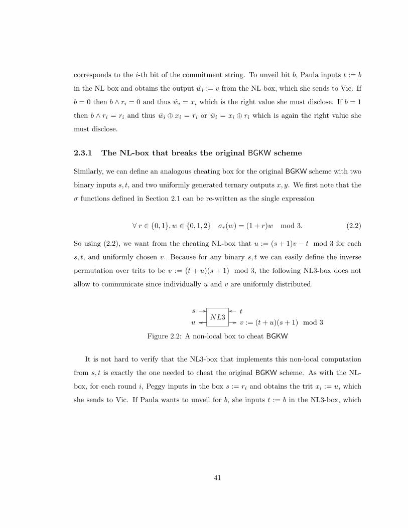
2.3.1 The NL-box that breaks the original BGKW scheme
Similarly, we can define an analogous cheating box for the original BGKW scheme with two
binary inputs s, t, and two uniformly generated ternary outputs x, y. We first note that the
σ functions defined in Section 2.1 can be re-written as the single expression
∀ r ∈ {0, 1}, w ∈ {0, 1, 2} σr(w) = (1 + r)w mod 3. (2.2)
So using (2.2), we want from the cheating NL-box that u := (s + 1)v − t mod 3 for each
s, t, and uniformly chosen v. Because for any binary s, t we can easily define the inverse
permutation over trits to be v := (t + u)(s + 1) mod 3, the following NL3-box does not
allow to communicate since individually u and v are uniformly distributed.
s //NL3
too
u //oo v := (t+ u)(s+ 1) mod 3
Figure 2.2: A non-local box to cheat BGKW
It is not hard to verify that the NL3-box that implements this non-local computation
from s, t is exactly the one needed to cheat the original BGKW scheme. As with the NL-
box, for each round i, Peggy inputs in the box s := ri and obtains the trit xi := u, which
she sends to Vic. If Paula wants to unveil for b, she inputs t := b in the NL3-box, which
41

correctly outputs wi := v. Clearly, they successfully cheat since
∀ i (1 + ri)wi − xi mod 3 = (1 + ri)(b+ xi)(1 + ri)− xi mod 3
= (1 + ri)2(b+ xi)− xi mod 3
= (b+ xi)− xi mod 3
= b.
2.4 Defining isolation
The existence of such an inputs-correlated1 random variable, which does not allow commu-
nication but allows cheating of the sBGKW two-prover bit commitment scheme sheds some
light on the original assumption of Ben-Or, Goldwasser, Kilian and Wigderson:
“Our construction does not assume that the verifier is polynomial time bounded.
The assumption that there is no communication between the two provers while
interacting with the verifier, must be made in order for the verifier to believe
the validity of the proofs. It need not be made to show that the interaction is
perfect zero-knowledge.”
Indeed this assumption is necessary but not sufficient to guarantee the binding property of
the bit commitment scheme. Among its weakness, we note that it does not explicitly force
any cheating strategy to be repeatable. Still, it is not hard to see that this was something
implicitly assumed in the proof of Theorem 2.3, when we wrote that in both cheating sce-
narios, a successful cheating end up in knowing wb for both b ∈ {0, 1}. The NL-box not
being a repeatable process2 gives a first understanding why we can still cheat the sBGKW
1We emphasize that at least one of the “inputs” to the random variable needs to be obtained once the
provers are isolated, otherwise such a random variable can be shared while the provers are together, and is
thus useless to cheat the sBGKW scheme.2Of course, the NL-box can be repeated as often as one wants. For instance, Peggy and Paula can easily
generate the output pair (x0, w0) from the input pair (r, 0), and the output pair (x1, w1) from the input
pair (r, 1), and all these outputs are individually uniformly distributed. However, Peggy can send only one
of x0 and x1 to Vic, and thus only the corresponding w will be valid on Paula’s side for unveiling. There
42

despite the result of Theorem 2.3.
Clearly, to achieve the binding condition a stronger assumption must be made. How-
ever, pin-pointing it precisely is not easy. At first sight, one could require the following
assumption:
“Once the provers are isolated, there exists no mechanism by which they may
sample a joint random variable which is dependent on inputs they provide.”
We note that, among other things, this new condition excludes communication between the
two provers, as desired. However, it excludes a lot more, such as shared entanglement! This
last observation is somewhat constraining as it forbids to Peggy and Paula the use of some
of the nicest properties of quantum mechanics. In a context where quantum processing is
used but entanglement is not allowed, some results (e.g [BBKM04, KMR05]) showed that
it is still possible to slightly outperform classical computations. Yet, it would be surprising
that this small separation from the classical setting is enough to cheat the sBGKW scheme.
Moreover, such a scenario is far fetch: to get interesting security results we need to consider
entanglement. This new assumption is simply too strong; we need to be more subtle in the
way we define this “mechanism to sample a joint random variable”.
It seems reasonable to believe that nature does not allow the existence of an NL-box as
described in Section 2.3 (that is, as a black-box or an implementation exponentially close
to a black-box). So why even ask for a stronger assumption than the no-communication
assumption of [BGKW88]? Part of the answer is that Vic can play the role of the NL-box,
or any other joint sampler. In no circumstances can we ignore the fact that both Peggy and
Paula individually talk to Vic. Definitely, we need to consider this aspect of the protocol
with great care. For instance, consider the scenario where r is sent to Peggy but commit-
ting and unveiling is not done immediately after, but rather once Vic and the two provers
have been involved in other, unrelated, interactive protocols. It is perfectly conceivable
is no way for them to force the relation x0 = x1. This means that, in our context, the NL-box cannot be
repeated to generate two valid strings w0 and w1.
43
that within those protocols, for each i, Peggy and Paula succeed in sending ri and b to Vic,
and then in a completely different context, or a moment of unawareness, Vic performs the
required computation and output xi and wi, which are then sent to respectively Peggy and
Paula. It is obvious that if such a computation, or any alike, can take place with enough
probability then Peggy and Paula would succeed in cheating the sBGKW protocol!
More generally, we must not only consider Vic but any other third party, call it Ted, to
which Peggy and Paula might have access to obtain correlated information. The previous
situation highlights the fact that there is a whole class of functions with inputs coming
from Peggy and Paula for which Ted must not send the outputs. Intuitively, each time Ted
sends a message to either Peggy or Paula, he must ensure that the message does not:
• allow Peggy and Paula to communicate;
• allow Peggy and Paula to achieve correlations better than what can be attained by
local variables if Peggy and Paula are classical players, or shared entanglement if they
are quantum provers.
That is, Ted must not outperform what Peggy and Paula can achieve using local vari-
ables in the sense of quantum mechanics. We wish to formulate that statement as a con-
venient computable criteria. A natural way to tackle the problem is to look at the entropy
of the message Ted is about to send conditioned on what was previously sent from and to
Ted. Suppose Ted is sending a message M to Peggy. Loosely speaking, if the uncertainty
about M is the same whether Peggy has access to Paula’s information or a local variable
independent of Paula’s information, then there is no problem sending M to Peggy because
she can produce M on her own. However, if there is less uncertainty when Paula’s infor-
mation is available, then it means that Peggy needs some information held by Paula to
produce this M with the same probability distribution. Hence, if Ted sends M , he gives
to Peggy a string with a probability distribution (correlations) she could not have obtained
otherwise. In the quantum case, the local variables are replaced by a quantum state, which
often allows more correlations between Peggy and Paula than local variables do. At this
44

point, we will not consider the quantum case.
The above gives the flavor of an information theoretic approach to the problem; this
is suitable as long as we stay at the variable level of a protocol. However, when Ted is
involved in some computations with Peggy and Paula, he his working with instances of
variables, and he may not know exactly, or have access to, the whole distribution from
which come the instances he receives from Peggy and Paula. Of course, running the same
computation multiple times on new instances would allow to re-generate the distribution of
each variable, but it would be much more practical to have a criteria from which Ted can
decide directly with the messages he has if he can send a message, or not. To this end, we
start by introducing the following criteria.
Let Peggy be represented by P0 and Paula by P1. The variable D ∈ {0, 1} is a reference
to player PD, and T ∈ {∅, {0}, {1}, {0, 1}} is a tag appended to each message that indicates
to Ted the player(s) that are eligible for receiving this message, where T = {0, 1} means by
both players and T = ∅ means by none of them. The message about to be sent from Ted
to prover PD is represented by (m,T )D. We formalize Ted’s behavior as follows.
Definition 2.1 (Practical definition) Ted is said to be a “secure third party” if ∀D ∈
{0, 1}, Ted follows these points.
1. A message received from player PD is tagged with T := {D}.
2. A message generated without involving any of the previous messages, e.g. picking a
random string, is tagged with T := {0, 1}.
3. A message obtained from a computation involving previous messages is tagged with
the intersection of the tags of all the messages involved in that computation.
4. A message (m,T )D is sent to player PD only if D ∈ T .
45

We now explain why Ted will not send a message that allows P0 and P1 to communicate
or establish non-local correlations. Let (m,T )D be the message Ted is about to send to
player PD. From the fourth point of Definition 2.1, Ted will send (m,T )D only if it is
tagged T = {D} or {0, 1}. Looking at the message’s tag assignment rule number 3, this
happens only if there is absolutely no message tagged {1 − D} or ∅ used in the compu-
tation of (m,T )D. Using an induction argument, it is not hard to see that this happens
only when all the variables involved in the computation of (m,T )D are independent of the
information of P1−D, that is, they have been themselves generated using variables tagged
{D} or {0, 1}. Thus, such a message (m,T )D is also independent of the information known
only to P1−D. Therefore, the messages sent by Ted do not let the two players communicate.
The case of non-locality is slightly more subtle, yet pretty straightforward. Recall that
in a general non-local process, both players use a message each and receive a message
uniformly distributed, from their point of view, such that the four messages satisfy a cer-
tain relation. The received message does not allow to communicate with the other player.
Suppose P1−D receives his message first. Since from his point of view, this message is uni-
formly distributed, Ted can in fact generate a uniformly distributed message, tag it with
T := {0, 1} and send it to P1−D. At this point, this behavior does not violate anything
because non-locality has not been created yet. Then, Ted computes the message for PD.
Because this message needs to satisfy the relation that binds together the four messages,
at least a message tagged with T 6= {D} and one tagged with T 6= {1 − D} are used in
its computation (it can be the same message), so the resulting message (m,T )D will be
assigned a tag T := ∅ because the intersection does not contain {D} and {1 − D}. This
message (m, ∅)D is the one creating the non-local relation. However, from point 4 of Defi-
nition 2.1, since D /∈ ∅, Ted will never send (m, ∅)D.
As mentioned before the previous definition, we can alternatively formalize Ted’s be-
havior in terms of entropy. Let the message about to be sent from Ted to prover PD be
represented by the variable (M,T )D. The set of variables SD,T represents all the variables
46
(messages) with tag T sent by prover PD to Ted, and the set of variables RD,T all the
variables (messages) with tag T sent by Ted to prover PD before (M,T )D.
Definition 2.2 (Information based definition) Ted is said to be a “secure third party”
if ∀D ∈ {0, 1}, Ted follows these points.
1. An information received from player PD is tagged with T := {D}3.
2. A variable M to be sent to PD is tagged with the less restrictive tag T ∈ {∅, {D}, {0, 1}}
that satisfies the following relation4,5. Note that the calligraphic tag T ′ stands for the
tag {0, 1}/(T∩{D}
)and the calligraphic tag T ′′ stands for the tag {D}∪
(T∩{1−D}
).
H((M,T )D|SD,{D}, RD,{D}, RD,{0,1}, S1−D,T ′ , R1−D,T ′ , R1−D,{0,1})
= H((M,T )D|SD,T ′′ , RD,T ′′ , RD,{0,1}, R1−D,{0,1}) (2.3)
3. A variable (M,T )D is sent to player PD only if D ∈ T .
We warn the reader that the tags and players’ variables D and 1−D do not play any
role in the computation of the entropies; they are only present to discriminate the variables
and determine which ones to include in the conditional part of the entropies. Notice also
that, contrary to Definition 2.1, a variable’s tag is set only when Ted consider sending it to a
player, except for incoming variables. This relaxation will turn out to be the key point to ex-
plain why this generalized definition is not stronger than local variables on the players’ side.
To strengthen the understanding, we first give an example of the application of this
definition using the relation of the NL-box. Recall that P0 has input X, P1 input Y 6,3This implies that the sets SD,{0,1} and S1−D,{0,1} are always empty. Therefore we did not include them
in equation (2.3), but a formal expression should include them in the conditional part on both sides of the
equality.4In order to write a clear equation, we had to specify to which player the message is intended. As a
result, we did not include {1−D} in the set of possible tags. It turns out that the empty set tag is sufficient
to cover both communication and correlation.5Explanations for equation (2.3) will be provided after the example of its application.6We are not using S and T for the variables’ name to avoid notation conflicts with the set S and tag T
used in Definition 2.2.
47
and they want to produce respectively a variable U and V such that the following relation
holds,
X ∧ Y = U ⊕ V.
Both players send their input to Ted, who tags them accordingly, i.e. (X, {0})0 and
(Y, {1})1. Suppose U is the first message to be sent. Recall from Section 2.3 that U
and V are individually uniformly distributed. Hence, Ted can pick U uniformly and send it
to P0, and U is tagged with {0, 1} 7. Then Ted would like to send V = U ⊕ X ∧ Y .
Let’s compute the left- and right-hand sides for the three possible tags. Notice that
S1,{1} = {(Y, {1})1}, S0,{0} = {(X, {0})0}, R0,{0,1} = {(U, {0, 1})0}, and all the other sets
are empty.
- If we set T := ∅, then T ′ = {0, 1} and T ′′ = {1}. The left-hand side is
H((V, ∅)1|S1,{1}, R1,{1}, R1,{0,1}, S0,{0,1}, R0,{0,1}) =
H((V, ∅)1|(Y, {1})1, (U, {0, 1})0) =12.
The right-hand side is
H((V, ∅)1|S1,{1}, R1,{1}, R1,{0,1}, R0,{0,1}) =
H((V, ∅)1|(Y, {1})1, (U, {0, 1})0) =12.
- If we set T := {1}, then T ′ = {0} and T ′′ = {1}. The left-hand side is
H((V, {1})1|S1,{1}, R1,{1}, R1,{0,1}, S0,{0}, R0,{0}, R0,{0,1}) =
H((V, {1})1|(Y, {1})1, (X, {0})0, (U, {0, 1})0) = 0.
The right-hand side is
H((V, {1})1|S1,{1}, R1,{1}, R1,{0,1}, R0,{0,1}) =
H((V, {1})1|(Y, {1})1, (U, {0, 1})0) =12.
7It is straightforward to verify that this is the less restrictive tag.
48

- If we set T := {0, 1}, then T ′ = {0} and T ′′ = {0, 1}. The left-hand side is
H((V, {0, 1})1|S1,{1}, R1,{1}, R1,{0,1}, S0,{0}, R0,{0}, R0,{0,1}) =
H((V, {0, 1})1|(Y, {1})1, (X, {0})0, (U, {0, 1})0) = 0.
The right-hand side is
H((V, {0, 1})1|S1,{0,1}, R1,{0,1}, S0,{0,1}, R0,{0,1}) =
H((V, {0, 1})1|(U, {0, 1})0) = 1.
Thus the equation (2.3) holds only when T := ∅. It follows from point 3 that Ted won’t
send V to P1, as expected.
The process of determining which tag to assign can be broken into two steps. We start
with the empty tag ∅. The first step is to decide whether we can add {D} to the tag, or not.
Notice that the right-hand side of equation (2.3) is the same for T ∈ {∅, {D}}. This results
from the calligraphic tag T ′′, which is equivalent to {D} in this case. On the other hand,
the calligraphic tag T ′ introduces the terms S1−D,{1−D} and R1−D,{1−D} in the left-hand
side of equation (2.3) when T = {D}. Thus, if the result of this first step is that the tag
is at least {D}, then it means that the message to be sent is independent of the private
information held by P1−D. However, if we find that the tag is not even {D}, then it means
that the message to be sent has some dependencies with the private information of P1−D,
and therefore the message should not be sent.
If the first step terminates with a tag containing at least {D}, then we can move on to
determine whether we can add {1−D} to the tag, or not. We note that T ′ won’t change
for T ∈ {{D}, {0, 1}}, so the left-hand side is invariant. However, the calligraphic tag T ′′
will remove the terms SD,{D} and RD,{D} from the right-hand side if we consider the tag
T = {0, 1}. Hence, if equation (2.3) is satisfied with T = {0, 1}, it means that the message
to be sent is not only independent of the private information of P1−D (from first step), but
also of the private information of PD. It follows naturally that this message be eligible for
49

distribution to both players.
The interest of Definition 2.2 is that it is more flexible in the tag assignation than
the practical definition 2.1. Indeed, whenever Ted deliberately randomizes a message with
new [uniformly distributed] information, the information-based tag assignment rule con-
clude that there is no problem to send to PD a message that would have been tagged with
T = {1−D} or ∅ in the practical definition. We give two examples of these particular cases.
Let P0 send to Ted a message represented by (X, {0})0 (the variable X is tagged with
{0} and comes from P0). Then Ted generates a uniform random variable (W,T )D (its tag
and receiver have not been set yet) and produces the message M = X⊕W for P1. Checking
with equation (2.3) we see there is no problem setting M’s tag to {1}, as
H((M, {1})1|(X, {0})0) = H((W,T )D) = H((M, {1})1).
This is satisfied since (W,T )D is uniform and has never been sent. However, the practical
definition would have assigned the tag T := {0} since W ’s tag would have been {0, 1} (by
the second rule) and {0} = {0} ∩ {0, 1}. Let Ted send (M, {1})1. We now get that for both
D = 0 and 1, if T = {D} or {0, 1} then the left-hand side of equation (2.3) for W is
H((W,T )D|(X, {0})0, (M, {1})1) = 0,
and the right-hand side is respectively
H((W, {0})0|(X, {0})0) = H((W, {0})0) = 1,
H((W, {1})1|(M, {1})1) = H((X, {0})0) = 1,
H((W, {0, 1})D) = 1.
Because equation (2.3) is not satisfied for both T = {D} and {0, 1}, W ’s tag is set to
T := ∅, and Ted should not send (W, ∅)D to neither of PD, for D = 0, 1.
Similarly, we can send to P1 a messageM that would have been tagged ∅ by the practical
definition. We again take the NL-box relation for example. Suppose the variables (X, {0})0
50

and (Y, {1})1 have already been sent to Ted by the players (and tagged accordingly), and
(U, {0, 1})0 8 has been sent by Ted to P0. Let (W,T )D be a uniformly distributed random
variable chosen by Ted, with D ∈ {0, 1}. Consider the following variable for P1,
V = U ⊕(W ⊕X
)∧ T,
that is, we randomized the variable tagged {0} (i.e. X) in the NL-box relation. In the
practical definition, because W is chosen uniformly and independently of previous variables,
the second rule would have assigned a tag {0, 1} to it, and so V ’s tag would have been set
to ∅ = {0, 1} ∩ {0, 1} ∩ {0} ∩ {1}. However, checking with equation (2.3), because W has
not been sent yet, we get that there is no problem setting V ’s tag to {1}, as
H((V, {1})1|(Y, {1})1, (X, {0})0, (U, {0, 1})0) =12
= H((V, {1})1|(Y, {1})1, (U, {0, 1})0).
So Ted would send this message (V, {1})1 to P1. Is this a problem? No, because the classical
limitations of non-locality have not be violated yet! The reason is simple: by randomizing
completely all the [private] variables related to P0, Ted is reducing the message he sends
to P1 to what P1 can exactly achieve using local variables. That is to say, P1 already
has a random view of P0’s variables, so there is no problem for Ted to first randomize P0’s
variables and then send this message to P1. If we make the calculations, we see that indeed,
for the variable V sent, the relation
V = U ⊕X ∧ Y
holds with probability 75%, just as in the classical scenario, and no W will never let us
beat that. Of course, as in the previous example, the variable (W,T )D used to randomize
can never be disclosed to any of the two players, and equation (2.3) agrees with that (W ’s
tag will be set to T := ∅ for both D).
Thus, if the message intended to PD is computed in such a way that it is independent of
S1−D,T and R1−D,T , for T ∈ {{0}, {1}, ∅}, i.e. it is randomized such that it no longer carries
8It is straightforward to verify that this is the less restrictive tag.
51

information that is known only to P1−D, then the criteria of Definition 2.2 does let Ted send
a message that would have been tagged {1−D} or ∅ in the practical definition. However,
the variables used to randomize such a message can never be disclosed to any of the players.
But this is correct since it is now these variables that carry the information dependent on
S1−D,T and R1−D,T , for T ∈ {{0}, {1}, ∅}. In this sense, Definition 2.2 is more general than
Definition 2.1 as it does not consider only the tag of a message to determine whether Ted
should send it, but rather its relevant information content. Moreover, Definition 2.2 does
let Ted send messages to the players that achieve the classical limitations of non-locality,
that is, Ted never sends a message that outperforms what the players can achieve with local
variables!
Henceforth, the two-prover model’s assumption is based on this refined definition of
isolation.
Definition 2.3 Peggy and Paula are isolated from one another if they cannot communicate
with one another, and for any third party Ted that interacts with Peggy and Paula, Ted is
a secure third party.
2.5 Fixing the proof of Theorem 2.3
We now prove the security of the sBGKW scheme with respect to this new definition. But
let’s first express the sBGKW scheme with the new terminology, to show that the protocol
can indeed be completed in the context of the practical definition of isolation.
sBGKW
P0 and P1 agree on an n-bit string w. They are then isolated from one another
according to Definition 2.3.
Commit to b:
- Vic sends a random n-bit string (r, {0, 1})0 to P0,
52
- P0 computes x := (b · r)⊕w and sends it to Vic. Upon reception, Vic
tags it (x, {0})0.
Unveil b:
- P1 announces b and an n-bit string w to Vic. Upon reception, Vic tags
them (b, {1})1 and (w, {1})1.
- Let e = 0 if “w = (b · r) ⊕ x”, and e = 1 otherwise. Vic accepts iff
e = 0, and tags e with (e, ∅)D for both D ∈ {0, 1}.
Since the only communication from Vic to the provers is a random n-bit string, it is straight-
forward that the protocol will complete with the new isolation assumption.
Theorem 2.4 Let Peggy (P0) and Paula (P1) be isolated as in Definition 2.3, then the
sBGKW is secure classically.
Proof : As before, the concealing condition is satisfied since Vic does not know w.
The previous section explained that in the setting of Definition 2.3, we are now guar-
anteed that any strategy that Peggy and Paula try to perform through a third party can
be achieved using only local variables on each side. We also know from Theorem 1.3 that
there’s no gain for Peggy and Paula to use a probabilistic strategy; we can thus assume,
without loss of generality, that a deterministic strategy is employed.
Suppose the two provers have a deterministic strategy that successfully produces w0
when they want to unveil as B = 0, and w1 when they want to unveil as B = 1. Because
we are dealing with classical information, the instances of the local variables and the infor-
mation of Peggy and Paula can be copied. From the deterministic behavior of the strategy,
their classical strategy can be run on each copy of the information to output both w0 and w1,
something we could not assert from only the no-communication assumption of [BGKW88].
Thus, any successful deterministic strategy would let Paula compute the string w0⊕w1 = r.
However r is completely unknown to her by the no-communication assumption. Therefore,
even using unlimited computational power, her probability of issuing a valid pair w0, w1 is
at most 1/2n. This proves that sBGKW is binding.
2
53

Chapter 3
Intermediate schemes towards
quantum secure bit commitment
We first exhibit two intermediate schemes to emphasize how shared entanglement can be
used to cheat with probability one (or almost one) a classically secure two-prover bit com-
mitment. The first protocol is a weaker version of the sBGKW scheme, called wBGKW,
where the acceptance criteria of the unveiling stage is loosen to tolerate some errors. The
second protocol is also a modified version of the sBGKW scheme where the acceptance
criteria is based on the Magic Square game (see Section 3.2).
3.1 A weaker acceptance criteria: the wBGKW scheme
We need the following notion.
Definition 3.1 The distance d(x, y) of a pair of binary words x, y is the number of bit-
positions where x and y differ.
In this section we consider a weaker version of sBGKW, called wBGKW, where the
acceptance criteria of the verifier Vic is to accept b and w if d(w, x ⊕ (b · r)) < n/5. This
means that the string w sent by Paula differs in at most n/5 positions from what it should
be. In comparison, in sBGKW the acceptance criteria is d(w, x ⊕ (b · r)) = 0. Note that
54

the choice of b is part of the expectation. The interest of such a modification is that now a
cheating quantum pair Peggy and Paula, isolated as in Definition 2.3, can use the non-local
property of entanglement to implement an NL-box and successfully cheat wBGKW, while,
as we show next, the bit commitment is secure classically. To facilitate notation we add an
index b to the string w, since w is different whether we unveil zero or one. Also, define as
B the random variable corresponding to the value they unveil.
Theorem 3.1 For any classical strategy, the probability that it outputs a string w0 when
B = 0 and w1 when B = 1 such that E[d(wb, x ⊕ (b · r))] < n/5 for both values of b, is
exponentially small in n.
Proof : Using the same arguments as in the proof of Theorem 2.4, we can assume the
provers use a deterministic strategy that may produce such a w0 when B = 0, and w1 when
B = 1, so they can in fact output both w0 and w1. Hence, Paula can compute the string
w0⊕w1. Recall that when d(wb, x⊕(b ·r)) = 0 then w0⊕w1 = r. We want to determine the
distance between w0 ⊕ w1 and r for this situation. From the theorem’s assumption, there
exists a classical strategy that outputs w0 and w1 such that E[d(wb, x⊕ (b · r))] < n/5, for
B = 0, 1. We easily obtain that for such a strategy, the expected distance from r is
E[d(w0 ⊕ w1, r)] = E[d(w0 ⊕ w1, x⊕ (x⊕ r))] ≤ E[d(w0, x)] + E[d(w1, x⊕ r)] < 2n/5
by the triangular inequality. Using a standard Chernoff Bound argument, and since r is
absolutely unknown to Paula, her probability of outputting a string z = w0 ⊕ w1 such that
E[d(z, r)] < (1/2 − ε) · n is exponentially small in n for any 0 < ε ≤ 1/4. Hence, because
2/5 < 1/2, we conclude that such a strategy cannot exist except with exponentially small
probability, and so unveiling must fail for one of the two possibilities.
2
Conversely, this scheme is almost totally insecure against quantum adversaries.
Theorem 3.2 There exists a quantum strategy that successfully cheats the wBGKW scheme
with probability 1− µ(n).
55
Proof : We saw in Section 2.3 that the NL-box, taken as a black box, correctly produced
the needed wb to unveil as b. Using the result of Theorem A.5 of Appendix A, we get
that through entanglement, Peggy and Paula can optimally simulate the NL-box such
that for each i taken independently, 1 ≤ i ≤ n, the NL-box produces correlated outputs
with probability cos2(π/8) ≈ 0.85. Therefore, using the standard Chernoff Bound, this
independent quantum strategy yields that for both values of b
E[d(w, x⊕ (b · r))] = (1− cos2(π/8)) · n,
with probability exponentially close to one. Having that
(1− cos2(π/8)) · n < 0.15 · n < n/5,
we conclude that a pair of quantum provers defeat the binding condition of the scheme with
probability 1− µ(n).
2
3.2 The Magic Square
The magic square game is a two-player pseudo-telepathy game that was presented by Pad-
manabhan Aravind [Ara02, Ara03], who built on work by Mermin [Mer90]. The most
interesting feature of this game is that it is extremely easy to show that there cannot be
a classical strategy that wins with probability one (see Section A.2.1). It follows that a
successful implementation of the quantum winning strategy (see Section A.2.2) would con-
vince any observer that something classically impossible is happening, with no need for the
observer to understand why the quantum strategy works.
3.2.1 The game
A magic square is a 3× 3 matrix whose entries are in {0, 1}, with the property that the sum
of each row is even and the sum of each column is odd. Such a square is magic because it
cannot exist! Indeed, suppose we calculate the parity of the nine entries, that is, the parity
56

of the whole square. This value is equal to the parity of the parities of the three rows and
equal to the parity of the parities of the three columns. However, according to the rows the
parity is even, yet according to the columns, the parity is odd! This is obviously impossible.
The task that the players face while playing the game is the following. Let x, y ∈
{0, 1, 2}. Peggy is asked to give the entries of the x-th row, labeled rx := rx0r
x1r
x2 , and Paula
is asked to give the entries of the y-th column, labeled cy := cy0cy1c
y2. To win the game,
the parity of the row rx must be even, the parity of the column cy must be odd, and the
intersection of the given row and column must agree, that is rxy = cyx.
Classical and quantum optimal strategies can be found in Section A.2 of Appendix A.
3.2.2 Magic Square bit commitment
The Magic Square bit commitment scheme, named MSBC, is an original idea due to Claude
Crepeau. This scheme is particularly relevant in our study of bit commitments in the two-
prover model as it is perfectly secure classically but can easily be cheated with probability
one using a quantum strategy. First, define the validity of a square.
Definition 3.2 A (3× 3) matrix Sx is valid for bit x if all rows of Sx xor to 0 when x = 0
and all columns of Sx xor to 1 when x = 1.
For instance the following matrix S0 is valid for zero while S1 is valid for one:
S0 =[
0 0 00 1 11 0 1
], S1 =
[1 0 11 1 01 0 0
]. (3.1)
The scheme is as follows.
MSBC
Peggy and Paula agree on a random n-bit string w and an identical random
square SPeggyi = SPaula
i for each bit wi of w such that Si is valid for wi. They
are then isolated as in Definition 2.3.
57

Commit to b:
- Vic chooses a random n-bit string a and sends it to Peggy. Label
a0 := 0n, the all 0’s n-bit string, and a1 := a.
- Peggy computes x := ab ⊕ w and sends x to Vic.
Unveil b:
- Peggy sends b to Vic.
- Vic computes w := ab ⊕ x.
- Vic challenges Peggy and Paula for each bit wi of w using a test on
the squares SPeggyi and SPaula
i . Vic picks a pair of random trits tPeggyi
and tPaulai and asks Peggy for row number tPeggy
i of SPeggyi and Paula
for column number tPaulai of SPaula
i .
- Vic accepts b if for each i, the row or column that should xor to wi
does, and if the intersection of the row and column is identical from
both Peggy and Paula. Vic rejects otherwise.
Note that this scheme does not differ much from the sBGKW scheme. Instead of having
Paula send explicitly w, both Peggy and Paula send information to Vic to allow him to
reconstruct w. Indeed, we can easily see that the magic squares are just a very redundant
version of w. If Vic sees all the magic squares of Peggy-Paula at unveiling, it is just repeat-
ing him what w was for each of Peggy and Paula. He can then compare this w to his w
and decide whether or not he should accept b.
We now prove that the MSBC is secure classically. It is straightforward to see that the
concealing property holds for Vic who does not know w.
Theorem 3.3 Any classical strategy successfully cheats the binding property of the MSBC
scheme with probability at most(
89
)n/6, except with exponentially small probability.
Proof : In order to cheat the bit commitment scheme, Peggy and Paula must be able to win
a weaker form of the Magic Square pseudo-telepathy game given in Section 3.2.1, where
58

for each i Vic verifies only that the row or column that should xor to wi does, instead
of verifying that the row xores to zero and the column xores to one. Using the result of
Theorem 1.3, we only need to consider deterministic strategies.
To simplify the proof, assume that Peggy always knows when she is being tested. The
probability of successfully cheating we will obtain under this assumption will be an upper
bound on the probability for any other strategy. One of the key point is that we cannot
make the same assumption regarding Paula: since she doesn’t know the random string
a1 := a sent by Vic to Peggy, she cannot tell whether she is being tested or not. Hence,
when she’s asked a column that does not xor to 1, she doesn’t know if she has to change
one of the bit to make it xor to 1.
However, Paula is using a deterministic strategy and Peggy knows all the information
possessed by Paula, except for the number tPaulai asked by Vic. This means that Peggy can
do the same computations as defined by Paula’s strategy to get the three possible columns
that Paula could output. Note that, put together, these three columns form a square S
which is the square that holds the most relevant information regarding Paula’s choices1.
Without lost of generality, we can thus assume that Paula always output a column that
xores to 1, and if needed, modifies the first bit of the column. So Paula always succeeds
her challenges. To simplify the proof further, we can assume that the last two rows of all
the squares SPeggyi = SPaula
i they share in the beginning of the protocol always xor to 0.
Consider a challenge i where Peggy is being tested (otherwise she simply outputs the
row tPeggyi asked by Vic and they succeed the challenge). As long as tPeggy
i = 1 or 2, she
can simply outputs the required row and succeed without being caught. However, with
probability 1/3, tPeggyi = 0, and from Paula’s strategy, this row xores to 1 in the square S
corresponding to the three possible columns answered by Paula. So Peggy has to modify1Hence, to maximize her probability of cheating, Peggy needs to base her strategy on S when returning
the row asked by Vic.
59
one bit of the row. With probability 1/3, she will modify the bit corresponding to the
column number tPaulai , and they will get caught. Therefore, for a challenge i, when Peggy
is being tested, their probability of success is at most 8/9.
By independence of the challenges, we get that the success probability is at most 8/9 for
each one where Peggy is being tested. Let x be the string sent by Peggy, prepared according
to the strategy of her choice. Since wi = x⊕ab, the test will toggle between Peggy and Paula
whenever ab = 1. The problem for Peggy is that whenever the test toggles, she can succeed
with certainty for at most only one of b ∈ {0, 1}. Since a is uniformly distributed, using a
Chernoff argument, except with exponentially small probability, the string a1 := a contains
n/3 1’s. Thus, there is at least one of b ∈ {0, 1} for which in at least n/6 challenges Peggy
will answer correctly with probability at most 8/9 (the sum of the challenges where she
succeeds with probability at most 8/9 for 0 and those where she succeeds with probability
at most 8/9 for 1 adds up to n/3). Therefore, their probability of successfully cheating is
at most (89
)n/6
for any classical strategy.
2
It follows that for n big enough, the MSBC scheme is binding. Conversely, this scheme is
totally insecure against quantum adversaries.
Theorem 3.4 There exists a quantum strategy that successfully cheats the MSBC scheme
with probability one.
Proof : Using the quantum strategy presented in Section A.2.2, a quantum pair Peggy-
Paula can always produce a row and column that satisfy the winning condition of the Magic
Square game (Section 3.2.1). Hence they can unveil for both values of b with probability
one.
2
60

Chapter 4
Quantum secure bit commitment
in the two-prover model
We now present the modified version of the sBGKW scheme, called the mBGKW scheme,
and prove its security against quantum adversaries. Although the two schemes are almost
identical, it turns out the proof against quantum provers is easier with the latter. The
security of the sBGKW and BGKW schemes will follow as a corollary of mBGKW’s security.
4.1 The scheme
mBGKW
Peggy and Paula agree on an n-bit string w. They are then isolated as in
Definition 2.3.
Commit to b:
- Vic sends two random n-bit strings r0, r1 to Peggy.
- Peggy replies with x := rb ⊕ w.
Unveil b:
- Paula announces an n-bit string w to Vic.
61
- Vic computes r := w ⊕ x. He accepts iff r ∈ {r0, r1} and deduces b
from r = rb.
4.2 mBGKW is secure against quantum adversaries
We want to show that the mBGKW scheme is secure against a quantum adversary. Clearly
the commitment is concealing because Vic does not know w. This means that there exists
w and w′ such that x = r0 ⊕ w = r1 ⊕ w′, and Vic cannot determine which of w or w′ has
been used. This is merely an application of the One-Time Pad (Vernam Cipher). We refer
the reader to [Sti05] for a complete proof of its security, which provides a nice information
theoretic argument why Vic cannot learn any information about rb.
Before diving into the formal proof that the binding property holds, let’s first sketch the
background intuition. We use Definition 1.4 to give the security argument for the binding
property. As in Definition 1.4, let p0 be the probability of successfully unveiling zero and p1
be the probability of successfully unveiling one. Imagine Peggy and Paula are able to open
B = 0 or B = 1 with a good probability of success. This means that Paula can announce
w0 such that r0 = w0 ⊕ x or w1 such that r1 = w1 ⊕ x, depending upon whether B = 0
or B = 1 is unveiled. We stress that, unlike in the classical scenario, even if they use a
deterministic1 quantum strategy to get w0 or w1, we cannot assert that Paula is able to
generate both, since quantum states cannot be copied (see [NC00], pages 24 and 532 for
details), so the process cannot be repeated exactly. It follows that with a quantum strategy,
we can always hope to have w0 and w1, but not both at the same time, with non-negligible
probability. We refer the reader to the introductory Section 1.2 for clarifications on this
important distinction with the classical setting, particularly with Definition 1.3.
Yet, the crucial observation on which our proof relies is the same as in the classical
case, namely that if Paula could simultaneously compute (w0, w1), then she would learn1The process (algorithm) can be deterministic, still the final result will be random, by the probabilistic
nature of quantum mechanics and measurements.
62
r0 ⊕ r1 = w0 ⊕ w1. Clearly, this should not be possible with probability higher than 2−n
since Paula does not have any information about r0 and r1 2. However, we will not use this
bound directly as the security marker, but rather as an optimal limit to upper bound the
equation p0 + p1 of Definition 1.4.
Ideally, one expects that for any cheating strategy
p0 + p1 ≤ 1 +12n, (4.1)
the bound achieved when Peggy and Paula are classical. However, it turns out this upper
bound is not so easy to reach; the analysis needed to produce an upper bound that tight
needs to be incredibly precise. Fortunately, as long as we get something bounded above by
1 + µ(n) the binding condition is satisfied. The consequence of the next lemma gives an
upper bound slightly weaker than (4.1) by about a square root distance to 1.
Define
p⊕ := Pr[Paula determines r0 ⊕ r1].
The next lemma relates p⊕ to p0 + p1. We show that whenever p0 + p1 is greater than
1 + ε, Paula can guess r0 ⊕ r1 with probability at least ε2. Then, exploiting the fact that
the probability p⊕ to determine r0⊕ r1 is 2−n, the binding condition will naturally follows.
Lemma 4.1 Assume Peggy and Paula have probability pb to open b successfully such that
p0 + p1 ≥ 1 + ε for ε > 0. Then, Paula can guess r0 ⊕ r1 with probability p⊕ ≥ ε2/4.
Proof : Assume without loss of generality that when the unveiling phase of mBGKW starts,
Paula holds the pure state |ψ〉 ∈ HN of dimension N ≥ 2n. Note that we do not need to
consider the whole bipartite state between Peggy and Paula since when the unveiling phase
starts, Peggy does no longer play an active role in the protocol and no communication is
allowed between the two; hence her system can be traced-out of the global Hilbert space.2Recall that no quantum process can send information from Peggy to Paula without communicating some
classical information. Therefore r0 ⊕ r1 remains uniformly distributed over {0, 1}n during the execution of
the whole protocol.
63
Moreover, by linearity, the proof also holds if |ψ〉 is replaced by a mixed state. Notice also
that, from the new model’s assumption (see Section 2.4), Peggy and Paula cannot do better
using a third party than what they can achieve with entanglement; the state |ψ〉 can thus
be seen as her part of the shared entangled state.
Generally speaking, Paula has two possible strategies depending upon the bit b she
wants to unveil. When B = 0, she applies a unitary transform U0 to |ψ〉 in order to get the
state |ψ0〉 := U0|ψ〉 that she measures in the computational basis {|w〉〈w|}w∈{0,1}n applied
to the first n qubits of |ψ0〉. When B = 1, she proceeds similarly with unitary transform
U1 allowing to prepare the state |ψ1〉 := U1|ψ〉. She then measures |ψ1〉 using the same
measurement as for B = 0. All general measurement can be realized in this fashion, this
is thus a general strategy for Paula. Notice that in the proof of Kent [Ken05], the use of
unitary transformations U0 and U1 is obscured by the fact that he works with projective
measurements. Notice also that the measurement on the first n qubits of |ψb〉 can alter-
natively be expressed by the measurement operators {|w〉〈w| ⊗ IM}w∈{0,1}n on the whole
state |ψb〉, where IM is the identity matrix on the system of dimension M = N/2n.
From the values r0, r1, x ∈ {0, 1}n announced by Vic and Peggy during the committing
phase, we define wb := rb ⊕ x as the string Paula has to announce in order to open b with
success. We have,
pb = 〈ψb|wb〉〈wb|ψb〉, (4.2)
which by assumption satisfies
p0 + p1 ≥ 1 + ε, ε > 0. (4.3)
Notice that 〈ψb|wb〉 is a generalized inner product3 since |wb〉 lives in a subspace of dimension
2n in HN . Therefore when wb is obtained, there is some state left in HN of dimension N/2n
which we label as |vb〉 (i.e. |ψb〉 has not been completely collapsed by the measurement).
3If |w〉 ∈ HM and |ψ〉 ∈ HN then for |ψ〉N =P
i αi|ai〉M ⊗ |bi〉N/M we define 〈w|ψ〉 =P
i αi〈w|ai〉|bi〉.
64

Thus, using (4.2) we can write |ψb〉 as
|ψb〉 =√pb|wb〉|vb〉+
√1− pb|w⊥b 〉, (4.4)
where ‖〈vb|〈wb|w⊥b 〉‖2 = 0. Note that the “state” |w⊥b 〉 has not necessarily a physical signi-
fication. It is simply a mathematical tool that allows us to conveniently carry the statistics.
We want to determine a lower bound for the probability p⊕. One possible way for Paula
to compute r0 ⊕ r1 is to obtain w0 and w1 individually. Again, one possible way to do this
is to use the following strategy:
1. Paula applies the strategy allowing to open B = 0 from |ψ0〉 = U0|ψ〉 resulting in
the state |ψ0〉 after the measurement in the computational basis {|w〉〈w|}w∈{0,1}n has
been performed on the first n qubits, and
2. Paula prepares |ψ1〉 := U1U†0 |ψ0〉 before applying again the measurement in the com-
putational basis {|w〉〈w|}w∈{0,1}n on the first n qubits.
Note that when preparing |ψ1〉, we applied U †0 before U1. This is to put back the state
|ψ0〉 as close as possible as the original state |ψ〉. From (4.3) and for N big enough, the
probability to measure w0 in the first step is not too small and so, by applying the inverse
of all the unitary transformations generated by U0, the state |ψ〉 we get before applying U1
is a good enough approximation of the original |ψ〉. Similarly we can say that the fidelity
F (|ψ〉, |ψ〉) is large enough. By invariance under unitary transformation, it follows that
|ψ1〉 approximates |ψ1〉 with the same fidelity F (|ψ〉, |ψ〉).
In the strategy described above, the probability to determine r0 ⊕ r1 is
p0 · pw1|w0.
As we said earlier, this is only one of the possible strategies to determine r0 ⊕ r1, thus
p⊕ ≥ p0 · pw1|w0.
65
Let us first find a lower bound on the probability pw1|w0to produce w1 given that w0 has
already been produced after step 1. Since w0 was obtained, the state |ψ0〉 is equal to
|w0〉|v0〉. We have,
|ψ1〉 = U1U†0 |ψ0〉
= U1U†0 |w0〉|v0〉
= U1
(U †
0
|ψ0〉√p0− U †
0
√1− p0
p0|w⊥0 〉
)(4.5)
= U1|ψ〉√p0− U1U
†0
√1− p0
p0|w⊥0 〉 (4.6)
=|ψ1〉√p0− U1U
†0
√1− p0
p0|w⊥0 〉 (4.7)
=1√p0
(√p1|w1〉|v1〉+
√1− p1|w⊥1 〉 − U1U
†0
√1− p0|w⊥0 〉
), (4.8)
where (4.5) follows from isolating |w0〉|v0〉 in (4.4), (4.6) and (4.7) are obtained by definition
of U0 and U1 respectively, and (4.8) also follows from (4.4). At this point, Paula applies
the measurement in the computational basis in order to obtain w1. Since we are interested
only in finding a lower bound, the probability to obtain w1 is minimized when U1U†0 |w⊥0 〉 =
|w1〉|v1〉. It easily follows that,
pw1|w0= 〈ψ1|w1〉〈w1|ψ1〉
≥ 1p0
(√p1 −
√1− p0
)2(4.9)
≥ 1p0
(√p1 −
√p1 − ε
)2 (4.10)
≥ ε2
4p0, (4.11)
where (4.9) follows from (4.8), (4.10) is obtained from (4.3), and (4.11) follows from a Taylor
expansion. Finally, (4.11) gives the desired result since
p⊕ ≥ p0 · pw1|w0≥ ε2
4.
2
Theorem 4.2 The binding condition of mBGKW satisfies p0 + p1 ≤ 1 + 1√2n−2
.
66

Proof : From the isolation assumption, we have
p⊕ =12n
.
Using the result from Lemma 4.1,
12n
≥ ε2
4=⇒ ε ≤ 1√
2n−2. (4.12)
It follows that the binding condition is satisfied: plugging (4.12) in (4.3), we get for any
cheating strategies
p0 + p1 ≤ 1 +1√
2n−2.
2
The next corollary summarizes the security of the mBGKW against a cheating pair
Peggy-Paula with access to quantum resources.
Corollary 4.3 If there exists an algorithm A that can cheat the mBGKW bit commitment
scheme with probabilities p0 +p1 ≥ 1+1/p(n), for every polynomials p(·) and all sufficiently
large n’s, then there exists an algorithm A′ that can predict an unknown n-bit string (r0⊕r1)
with probabilities 1/4p(n)2, which is impossible.
Indeed the following stronger statement is also true:
Corollary 4.4 If there exists an algorithm A that can cheat the mBGKW bit commitment
scheme with probabilities p0 + p1 > 1 + (1/√
2)n then there exists an algorithm A′ that
can predict an unknown n-bit string (r0 ⊕ r1) with probabilities better than 1/2n, which is
impossible.
Notice the square root gap between the intuitively expected binding condition 1 + 12n
and the proven result of Corollary 4.4. This is merely the consequence of the crude lower
bound we found for p⊕. A more precise analysis covering more strategies to compute r0⊕r1
and results on the maximum information we can extract from optimal measurement on |ψ〉
might close the gap. Nevertheless, this small hole is not important enough to compromise
67

the security of the mBGKW scheme because the binding condition is still exponentially close
to one.
Notice also that the proof presented in Lemma 4.1 can easily be generalized to a whole
class of bit commitment schemes with the properties that information unknown to Paula
is sent to Peggy to commit, and an exact answer is needed from Paula to unveil success-
fully the committed bit. Corollary 4.4 therefore holds for a whole class of bit commitment
scheme in the two-prover model.
Note finally that sBGKW is the same as mBGKW where r0 := 000...0 is the all-zero
string all the time. The statement and proof of Lemma 4.1 is equally valid for any fixed
choice of either (but not both) r0 or r1 because the probability to predict r0 ⊕ r1 remains
exponentially small. Hence using only the model’s assumption we get
Corollary 4.5 If there exists an algorithm A that can cheat the sBGKW bit commitment
scheme with probabilities p0 + p1 > 1 + (1/√
2)n then there exists an algorithm A′ that can
predict an unknown n-bit string r with probabilities better than 1/2n, which is impossible.
4.3 Reduction to the original BGKW scheme
Building on Corollary 4.5, we can easily derive a similar result for the original BGKW
scheme. Consider the following reduction from the BGKW scheme to the sBGKW scheme.
First, Peggy and Paula perform their cheating algorithm for the BGKW scheme as usual.
Suppose they successfully cheat for b; check Section 2.3.1 and Figure 2.2 to get a flavor of
what a successful strategy is supposed to output. For each bit of the random string r and
choice of bit b, Peggy receives the trit xi and Paula receives the trit yi := (ri + 1)(b + xi)
mod 3 from their strategy. They then convert these trits into bits to answer the sBGKW
scheme, as follows:
1. Peggy sends the bit x′i :=((ri + 1)xi mod 3
)mod 2.
2. Paula sends the bit y′i :=(yi + 2b mod 3
)mod 2.
68
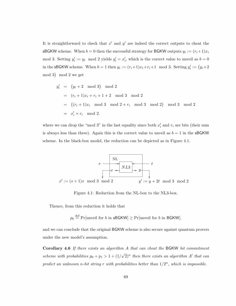
It is straightforward to check that x′ and y′ are indeed the correct outputs to cheat the
sBGKW scheme. When b = 0 then the successful strategy for BGKW outputs yi := (ri+1)xi
mod 3. Setting y′i := yi mod 2 yields y′i = x′i, which is the correct value to unveil as b = 0
in the sBGKW scheme. When b = 1 then yi := (ri+1)xi+ri+1 mod 3. Setting y′i :=(yi+2
mod 3)
mod 2 we get
y′i =(yi + 2 mod 3
)mod 2
= (ri + 1)xi + ri + 1 + 2 mod 3 mod 2
=((ri + 1)xi mod 3 mod 2 + ri mod 3 mod 2
)mod 3 mod 2
= x′i + ri mod 2.
where we can drop the “mod 3” in the last equality since both x′i and ri are bits (their sum
is always less than three). Again this is the correct value to unveil as b = 1 in the sBGKW
scheme. In the black-box model, the reduction can be depicted as in Figure 4.1.
NLs //
NL3oo t
x //oo y
�� ��x′ := (s+ 1)x mod 3 mod 2 y′ := y + 2t mod 3 mod 2
Figure 4.1: Reduction from the NL-box to the NL3-box.
Thence, from this reduction it holds that
pbdef= Pr[unveil for b in sBGKW] ≥ Pr[unveil for b in BGKW],
and we can conclude that the original BGKW scheme is also secure against quantum provers
under the new model’s assumption.
Corollary 4.6 If there exists an algorithm A that can cheat the BGKW bit commitment
scheme with probabilities p0 + p1 > 1 + (1/√
2)n then there exists an algorithm A′ that can
predict an unknown n-bit string r with probabilities better than 1/2n, which is impossible.
69
Conclusion and open problems
In this thesis we have shown that the long-standing assumption of no-communication be-
tween the two provers was not sufficiently precise to preserve the binding property of a
bit commitment scheme against all possible attacks. An extra assumption concerning the
verifier, and more generally any third party the two provers may have access to, needs to
be made to prevent him to send correlated messages to the provers, even if those messages
do not allow to explicitly communicate. This refinement has been formally modeled with
Definition 2.1.
The questions whether there exists classically secure commitment schemes that are
insecure against quantum provers, and whether there exists commitment schemes secure
against quantum provers, have both found affirmative answers. Once again, this highlights
the fact that even in the two-prover model, the question as whether a classically secure
commitment scheme is also secure against quantum adversaries is non-trivial. Indeed, we
have presented two schemes, the wBGKW and MSBC schemes, that can be cheated with
probability one, or exponentially close to one, if the provers share entanglement. On the
other hand, we also presented a scheme, the mBGKW scheme, for which a proof that no
quantum strategy can cheat the commitment was given. The security of the original BGKW
commitment scheme has been proved by reduction from the security of the mBGKW scheme.
A natural question with respect to our new model’s assumption is how can it be loos-
ened. Actually, it forbids Peggy an Paula to have access to any kind of non-local boxes
70

(which may be perfectly implemented through a third party); however such a strong re-
striction does not necessarily need to be imposed. Take for instance the sBGKW scheme in
the classical setting. Permitting Peggy and Paula to have access to a non-local box for the
Magic Square game would not give them the ability to cheat the commitment scheme: if
instead of the non-local box we let them have the entanglement that implements perfectly
such a box (see Section A.2.2), something that makes them strictly more powerful, then we
know from Lemma 4.1 that it does not help them to cheat. Still, our model’s assumption
does not allow such an inconsequential box! So how can the assumption be further refined?
Which boxes can we allow in the assumption, and which can we not? How can we prove
that a non-local box is futile without invoking Lemma 4.1?
The various applications of the sBGKW scheme also need to be studied. A direct conse-
quence of its security against quantum adversaries is probably the possibility to elaborate
quantum zero-knowledge proofs in the two-prover model. Using simple classical techniques
from [BGG+89] and [IY87] its seems rather straightforward for the two provers to prove in
zero-knowledge any statements in IP=PSPACE. However, as discussed in the introduction,
up to which complexity class it is possible to do so is not known, unless the amount of
entanglement shared between the provers is bounded by some a priori fixed polynomial in
the input length.
Questions like is it possible to build a quantum oblivious transfer protocol using the
construction of [CK88, Cre97], or a quantum mutual identification protocol as in [CS95]
are also intriguing. Determining if the quantum scheme presented in Section 4.2 is binding
with respect to the stronger Definition 1.5 is still an open problem.
71

Appendix A
Classical and quantum optimal
implementation of the NL-box and
the Magic Square game
Since its discovery by Einstein, Podolsky and Rosen, in the famous “thought experiment”
of [EPR35], and taking all its profound fundamentality with the controversial result of John
Bell in 1964 [Bel64], non-locality and its impact has been one of the major line of research
in quantum mechanics. As presented in [NC00],
“ [...] substantial experimental evidence together with the large set of inequalities
generically known as the Bell inequalities showed that non-local correlations are
a fundamental difference between classical and quantum physics, often referred
as the non-classical property of quantum mechanics.”
On a more practical hand, in quantum computation and information, non-locality is intro-
duced as entanglement shared between two (or more) parties. It is surprising to see how
non-locality can be exploited as a resource to perform information processing task impos-
sible using classical physic, e.g. quantum teleportation [BBC+93] and superdense coding
[BW92].
72
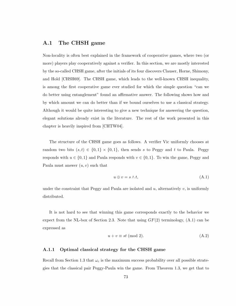
A.1 The CHSH game
Non-locality is often best explained in the framework of cooperative games, where two (or
more) players play cooperatively against a verifier. In this section, we are mostly interested
by the so-called CHSH game, after the initials of its four discovers Clauser, Horne, Shimony,
and Hold [CHSH69]. The CHSH game, which leads to the well-known CHSH inequality,
is among the first cooperative game ever studied for which the simple question “can we
do better using entanglement” found an affirmative answer. The following shows how and
by which amount we can do better than if we bound ourselves to use a classical strategy.
Although it would be quite interesting to give a new technique for answering the question,
elegant solutions already exist in the literature. The rest of the work presented in this
chapter is heavily inspired from [CHTW04].
The structure of the CHSH game goes as follows. A verifier Vic uniformly chooses at
random two bits (s, t) ∈ {0, 1} × {0, 1}, then sends s to Peggy and t to Paula. Peggy
responds with u ∈ {0, 1} and Paula responds with v ∈ {0, 1}. To win the game, Peggy and
Paula must answer (u, v) such that
u⊕ v = s ∧ t, (A.1)
under the constraint that Peggy and Paula are isolated and u, alternatively v, is uniformly
distributed.
It is not hard to see that winning this game corresponds exactly to the behavior we
expect from the NL-box of Section 2.3. Note that using GF (2) terminology, (A.1) can be
expressed as
u+ v ≡ st (mod 2). (A.2)
A.1.1 Optimal classical strategy for the CHSH game
Recall from Section 1.3 that ωc is the maximum success probability over all possible strate-
gies that the classical pair Peggy-Paula win the game. From Theorem 1.3, we get that to
73
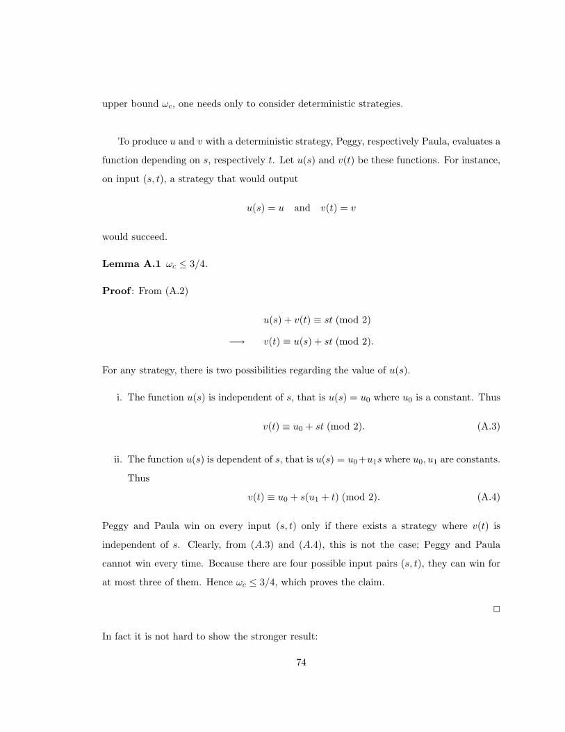
upper bound ωc, one needs only to consider deterministic strategies.
To produce u and v with a deterministic strategy, Peggy, respectively Paula, evaluates a
function depending on s, respectively t. Let u(s) and v(t) be these functions. For instance,
on input (s, t), a strategy that would output
u(s) = u and v(t) = v
would succeed.
Lemma A.1 ωc ≤ 3/4.
Proof : From (A.2)
u(s) + v(t) ≡ st (mod 2)
−→ v(t) ≡ u(s) + st (mod 2).
For any strategy, there is two possibilities regarding the value of u(s).
i. The function u(s) is independent of s, that is u(s) = u0 where u0 is a constant. Thus
v(t) ≡ u0 + st (mod 2). (A.3)
ii. The function u(s) is dependent of s, that is u(s) = u0+u1s where u0, u1 are constants.
Thus
v(t) ≡ u0 + s(u1 + t) (mod 2). (A.4)
Peggy and Paula win on every input (s, t) only if there exists a strategy where v(t) is
independent of s. Clearly, from (A.3) and (A.4), this is not the case; Peggy and Paula
cannot win every time. Because there are four possible input pairs (s, t), they can win for
at most three of them. Hence ωc ≤ 3/4, which proves the claim.
2
In fact it is not hard to show the stronger result:
74

Theorem A.2 ωc = 3/4.
Proof : Consider the truth table.
s t s ∧ t
0 0 0
0 1 0
1 0 0
1 1 1
The strategy where
u(s) = 0 and v(t) = 0
always output u(s)⊕v(s) = 0. It is straightforward that this strategy wins the CHSH game
3/4 of the time.
2
Among other things, the result of Theorem A.2 means that the NL-box cannot be simulated
perfectly using local variables on each side.
A.1.2 Optimal quantum strategy for the CHSH game
We now turn to the scenario where Peggy and Paula are allowed to use a quantum strategy.
We show that sharing entanglement, Peggy and Paula can beat the classical bound of 3/4.
As in [CHTW04], consider this specific strategy. Peggy and Paula share the entangled one
qubit state
|Φ+〉 =1√2
(|00〉+ |11〉
).
Define
|ψ0(θ)〉 := cos(θ)|0〉+ sin(θ)|1〉,
|ψ1(θ)〉 := sin(θ)|0〉 − cos(θ)|1〉.
75

Given s, Peggy will perform a projective measurement determined by the measurement
operators {Xus | u ∈ {0, 1}} and report u to Vic. Likewise, given t, Paula will perform a
projective measurement determined by the operators {Y vt | v ∈ {0, 1}} and send v to Vic.
Let the operators be
Xu0 = |ψu(0)〉〈ψu(0)|,
Xu1 = |ψu(π/4)〉〈ψu(π/4)|,
Y v0 = |ψv(π/8)〉〈ψv(π/8)|,
Y v1 = |ψv(−π/8)〉〈ψv(−π/8)|.
To prove this quantum strategy outperforms ωc, we need the following little identity.
Lemma A.3 Let |ϕ〉 ∈ Cd ⊗ Cd be any maximally entangled state, then for any d × d
complex matrix X (X ⊗ I
)|ϕ〉 =
(I ⊗XT
)|ϕ〉.
Proof : Using the Schmidt decomposition, the maximally entangled state |ϕ〉 can be ex-
pressed as
|ϕ〉 =1√d
d−1∑j=0
|j〉|j〉.
Similarly, the d× d complex matrix X can be expressed as
X =d−1∑k=0
d−1∑l=0
λkl|k〉〈l| λkl ∈ C.
Using some elementary linear algebra,
(X ⊗ I
)|ϕ〉 =
1√d
d−1∑j=0
d−1∑k=0
d−1∑l=0
λkl|k〉〈l|j〉|j〉
=1√d
d−1∑k=0
d−1∑l=0
λkl|k〉|l〉. (A.5)
76
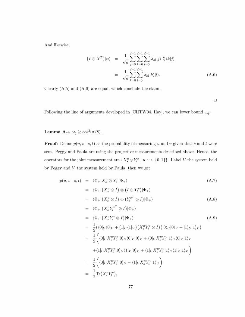
And likewise,
(I ⊗XT
)|ϕ〉 =
1√d
d−1∑j=0
d−1∑k=0
d−1∑l=0
λkl|j〉|l〉〈k|j〉
=1√d
d−1∑k=0
d−1∑l=0
λkl|k〉|l〉. (A.6)
Clearly (A.5) and (A.6) are equal, which conclude the claim.
2
Following the line of arguments developed in [CHTW04, Hay], we can lower bound ωq.
Lemma A.4 ωq ≥ cos2(π/8).
Proof : Define p(u, v | s, t) as the probability of measuring u and v given that s and t were
sent. Peggy and Paula are using the projective measurements described above. Hence, the
operators for the joint measurement are {Xus ⊗Y v
t | u, v ∈ {0, 1}}. Label U the system held
by Peggy and V the system held by Paula, then we get
p(u, v | s, t) = 〈Φ+|Xus ⊗ Y v
t |Φ+〉 (A.7)
= 〈Φ+|(Xu
s ⊗ I)⊗(I ⊗ Y v
t
)|Φ+〉
= 〈Φ+|(Xu
s ⊗ I)⊗(Y vT
t ⊗ I)|Φ+〉 (A.8)
= 〈Φ+|(Xu
s YvT
t ⊗ I)|Φ+〉
= 〈Φ+|(Xu
s Yvt ⊗ I
)|Φ+〉 (A.9)
=12(〈0|U 〈0|V + 〈1|U 〈1|V
)(Xu
s Yvt ⊗ I
)(|0〉U |0〉V + |1〉U |1〉V
)=
12
(〈0|UXu
s Yvt |0〉U 〈0|V |0〉V + 〈0|UXu
s Yvt |1〉U 〈0|V |1〉V
+〈1|UXus Y
vt |0〉U 〈1|V |0〉V + 〈1|UXu
s Yvt |1〉U 〈1|V |1〉V
)=
12
(〈0|UXu
s Yvt |0〉U + 〈1|UXu
s Yvt |1〉U
)=
12Tr(Xu
s Yvt
),
77
where (A.7) is by definition of measurement, (A.8) is by applying the identity of Lemma A.3
and (A.9) is because, given our particular choice of measurement operators for Paula, Y vt
is invariant under transpose. It is now routine to check that for every pair of inputs (s, t),
Peggy and Paula give the correct answer with probability cos2(π/8). As an example, we
do the case where (s, t) = (1, 1). Because s ∧ t = 1, Peggy and Paula need (u, v) ∈
{(0, 1), (1, 0)}. The first pair gives
p(0, 1 | 1, 1) =12Tr(X0
1Y11
)=
12Tr(|ψ0(π/4)〉〈ψ0(π/4)||ψ1(−π/8)〉〈ψ1(−π/8)|
)=
12|〈ψ0(π/4)|ψ1(−π/8)〉|2 by cyclicity of the trace
=12|(cos(π/4)〈0|+ sin(π/4)〈1|)(sin(−π/8)|0〉 − cos(−π/8)|1〉)|2
=12| − cos(π/4) sin(π/8)− sin(π/4) cos(π/8)|2
=12| − sin(π/4 + π/8)|2 =
12| − cos(π/2− π/4− π/8)|2
=12
cos2(π/8).
Doing the calculations, (u, v) = (1, 0) also gives p(1, 0 | 1, 1) = 1/2 cos2(π/8). Therefore the
probability to win when (s, t) = (1, 1) is 12 cos2(π/8) + 1
2 cos2(π/8) = cos2(π/8). The same
holds for the three other sets of inputs (s, t).
2
Theorem A.5 ωq = cos2(π/8).
Proof : The intuition behind what follows is that a strategy that could do better than
cos2(π/8) would require more “power” from entanglement. Our goal is then to show that
the strategy presented above exploits entanglement’s correlations to its maximum.
First, let us translate the measurement operators Xus , Y
vt into observables with eigen-
values ±1 ([NC00] p. 87). It is straightforward from its definition that the projector Xu0
corresponds exactly to a measurement in the computational basis {|0〉〈0|, |1〉〈1|}. Consider
the observable Z,
Z =
1 0
0 −1
= |0〉〈0| − |1〉〈1|. (A.10)
78

If Peggy applies the observable Z to her part of |Φ+〉, if she obtains the eigenvalue 1 it
means her part of |Φ+〉 has been projected in the state |0〉〈0|. On the other hand, if she
obtains the eigenvalue -1 it means her part of |Φ+〉 has been projected in the state |1〉〈1|.
One easily realizes that this has the same effect as applying the measurement {|0〉〈0|, |1〉〈1|}.
The measurement operator Xu1 corresponds to a measurement in the diagonal basis
{H|0〉〈0|H,H|1〉〈1|H}. We know from a simple calculation ([NC00] p. 459) that
HZH = X.
Hence, using the expression for Z in (A.10),
X = H|0〉〈0|H −H|1〉〈1|H.
As it was the case for the observable Z, the eigenvalue obtained after applying the observable
X has the same effect on the observed state as a measurement in the diagonal basis. Using
the same type of reasoning, we get that the observable for a general rotation Rθ by angle
θ is defined by
RθZRθ =
cos(θ) sin(θ)
sin(θ) − cos(θ)
·
1 0
0 −1
·
cos(θ) sin(θ)
sin(θ) − cos(θ)
=
cos2(θ)− sin2(θ) 2 cos(θ) sin(θ)
2 cos(θ) sin(θ) −(cos2(θ)− sin2(θ))
=
cos(2θ) sin(2θ)
sin(2θ) − cos(2θ)
.
Thus, the observable Y0 associated with the measurement in basis defined by Y v0 is
Y0 = Rπ/8ZRπ/8 =1√2
1 1
1 −1
=Z +X√
2.
and the observable Y1 associated with the measurement in basis defined by Y v1 is
Y1 = R−π/8ZR−π/8 =1√2
1 −1
−1 −1
=Z −X√
2.
79

To summarize, upon reception of (s, t) Peggy and Paula perform their measurement
using the observables
X0 = Z, Y0 =Z +X√
2,
X1 = X, Y1 =Z −X√
2.
Plugging these observables in the famous Bell inequality known as the CHSH inequality,
we get
〈X0Y0〉+ 〈X1Y0〉+ 〈X1Y1〉 − 〈X0Y1〉 = 2√
2, (A.11)
where 〈XiYj〉 = 〈Φ+|Xi ⊗ Yj |Φ+〉 denotes the mean value of Xi and Yj ; see [NC00] p. 116
for more details.
But wait! Using Tsirel’son [Cir80, Cir87] upper bound1 for any observable (X0 and X1
being applied by Peggy and Y0 and Y1 by Paula)
〈X0Y0〉+ 〈X1Y0〉+ 〈X1Y1〉 − 〈X0Y1〉 ≤ 2√
2,
we get that our strategy already uses the maximum out of the correlations produced by
entanglement. This conclude the theorem since no other strategy can do better.
2
A.2 The Magic Square game
A description of the Magic Square game can be found in Section 3.2.1.
For the interested reader, there are other pseudo-telepathy games that are related to
the magic square game. Adan Cabello’s game [Cab01b, Cab01a] does not resemble the
magic square game on first approach. However, closer analysis reveals that the two games
are totally equivalent! A formal proof of this claim can be found in [Bro04], along with the1Although Tsirel’son proved is bound using the singlet state 1√
2(|01〉− |10〉), a generalization by Wehner
[Weh06] showed it holds for any bipartite state.
80

definition of equivalence between pseudo-telepathy games.
Furthermore, Aravind has generalized his own magic square idea [Ara03] to a two-player
pseudo-telepathy game in which the players share n Bell states, n being an arbitrary odd
number larger than one.
A.2.1 Optimal strategy for classical players
Theorem A.6 When restricted to classical strategies, Peggy and Paula can win the Magic
Square game with probability at most 89 .
Proof : Using Theorem 1.3, we only have to consider deterministic strategies to establish
a bound for ωc(G), the maximum success probability of winning when the game G is the
Magic Square game.
A deterministic classical strategy would have to assign definite binary values to each of
the nine entries of the magic square. From our set of winning conditions (see Section 3.2.1),
it implies that the parity of the nine entries is even according to the rows and odd according
the columns. Obviously, no such set of entries can exist, so ωc(G) < 1. Using Lemma 1.4,
we get that ωc(G) ≤ 89 .
Consider the following square and associated deterministic strategy.
0 1 2
0
1
2
0 0 0
0 0 0
1 1 ?
The parity of rows zero and one is even, and the parity of columns zero and one is odd, so
Peggy and Paula win every time for these four possible cases without changing anything. If
Peggy is asked row two, then she changes the ? of entry (2,2) to zero to get an even parity,
and similarly Paula changes it to one to get a odd parity for column two. It is not hard
81

to see that they get caught cheating only when the intersection of the answered row and
column is the entry (2,2). Therefore ωc(G) = 89 , which conclude the proof together with
Lemma 1.2.
2
A.2.2 Quantum winning strategy
The quantum winning strategy for the magic square game is not as simple as the classical
impossibility proof. We refer the reader to [Ara02, Bro04] for a clear and detailed proof,
since we will present here only a swift overview.
Let Peggy and Paula share the entangled state
|ψ〉 = 12 |0011〉 − 1
2 |0110〉 − 12 |1001〉+ 1
2 |1100〉 . (A.12)
The first two qubits belong to Peggy and the last two to Paula. Upon receiving their inputs
x and y from the verifier Vic, Peggy and Paula apply respectively the unitary transformation
Rx and Cy, according to the following matrices. Note that, as a reminder, we used Rx as
the transformation associated with the computation for the row, and Cy for the column.
R0 =1√2
[ ı 0 0 10 −ı 1 00 ı 1 01 0 0 ı
], R1 = 1
2
[ ı 1 1 ı−ı 1 −1 ı
ı 1 −1 −ı−ı 1 1 −ı
], R2 =
12
[−1 −1 −1 11 1 −1 11 −1 1 11 −1 −1 −1
],
C0 =12
[ ı −ı 1 1−ı −ı 1 −1
1 1 −ı ı−ı ı 1 1
], C1 = 1
2
[−1 ı 1 ı1 ı 1 −ı1 −ı 1 ı
−1 −ı 1 −ı
], C2 =
1√2
[ 1 0 0 1−1 0 0 1
0 1 1 00 1 −1 0
].
Then, Peggy and Paula measure their qubits in the computational basis. This provides
two bits to each player, which are the first two bits of their respective output rx and cy.
Finally, Peggy and Paula determine their third output bit from the first two, so that their
parity condition is satisfied. The intersection condition is also always satisfied.
Consider for example inputs x = 1 and y = 2. After Peggy and Paula apply R1 and C2,
82

respectively, the state evolves to
(R1 ⊗ C2)|ψ〉 = 12√
2
[|0000〉 − |0010〉 − |0101〉+ |0111〉 (A.13)
+|1001〉+ |1011〉 − |1100〉 − |1110〉]. (A.14)
Suppose for instance that after measurement, Peggy and Paula obtained 10 and 01. In that
case, Peggy would complete with bit one so that her output r1 = 101 has even parity and
Paula would complete with bit zero so that her output c2 = 010 has odd parity. Vic will
be satisfied with the answer since both Peggy and Paula agree that the third entry of the
second row is indeed the same as the second entry of the third column: c21 = r12 = 1. It is
easy to check that the seven other possible answers that Peggy and Paula could have given
on this example are all appropriate. The verification that this quantum strategy wins also
on the other eight possible questions is tedious but straightforward.
83
Bibliography
[Ara02] P. K. Aravind. Bell’s theorem without inequalities and only two distant ob-
servers. Foundation of Physics Letters, pages 397–405, 2002.
[Ara03] P. K. Aravind. A simple demonstration of Bell’s theorem involving two ob-
servers and no probabilities or inequalities. ArXiv Quantum Physics e-prints
quant-ph/0206070, 2003.
[BB84] C. H. Bennett and G. Brassard. Quantum cryptography: Public key distri-
bution and coin tossing. In Proceedings of IEEE international Conference on
Computers, Systems and Signal Processing, Bangalore, India, pages 175-179,
New York, 1984. IEEE Press.
[BBC+93] C. H. Bennett, G. Brassard, C. Crepeau, R. Jozsa, A. Peres, and W. Wootters.
Teleporting an unknown quantum state by dual classical and EPR channel.
Physical Review Letter, volume 70, pages 1895–1898, 1993.
[BBKM04] E. Biham, G. Brassard, D. Kenigsberg, and T. Mor. Quantum computation
without entanglement. Theoretical Computer Science, volume 320, pages 13–
33, 2004.
[BC90] G. Brassard and C. Crepeau. Quantum bit commitment and coin tossing pro-
tocols. In Crypto ’91, volume 537 of Lecture Notes in Computer Science, pages
49–61. Springer, 1990.
84

[BCC88] G. Brassard, D. Chaum, and C. Crepeau. Minimum disclosure proofs of knowl-
edge. In Journal of Computer System Science, volume 37, pages 156–189, 1988.
[BCJL93] G. Brassard, C. Crepeau, R. Josza, and D. Langlois. A quantum bit com-
mitment scheme provably unbreakable by both parties. In Proceedings of the
34th Annual IEEE Symposium on the Foundations of Computer Science, pages
362-371, Los Alamitos, CA, 1993. IEEE Computer Science Press.
[BCMS98] G. Brassard, C. Crepeau, D. Mayers, and L. Salvail. Defeating classical bit
commitment schemes with a quantum computer. ArXiv Quantum Physics e-
prints quant-ph/9806031, 1998.
[Bel64] J. S. Bell. On the Einstein Podolsky Rosen paradox. Physics, volume 1, number
3, pages 195–200, 1964.
[BFL90] L. Babai, L. Fortnow, and C. Lund. Non-deterministic exponential time has
two-prover interactive protocols. Technical report, Chicago, IL, USA, 1990.
[BGG+89] M. BenOr, O. Goldreich, S. Goldwasser, J. Hastad, J. Kilian, S. Micali, and
P. Rogaway. Everything provable is provable in zero-knowledge. In Springer-
Verlag, editor, Advances in Cryptology, Crypto ’88, volume 403, pages 37–56,
1989.
[BGKW88] M. BenOr, S. Goldwasser, J. Kilian, and A. Widgerson. Multi-prover interactive
proofs: how to remove intractability. In STOC ’88: Proceedings of the twentieth
annual ACM symposium on Theory of computing, pages 113–131, New York,
NY, USA, 1988. ACM Press.
[BGW88] M. BenOr, S. Goldwasser, and A. Widgerson. Completeness theorems for non-
cryptographic fault-tolerant distributed computation. In STOC ’88: Proceed-
ings of the twentieth annual ACM symposium on Theory of computing, pages
1–10, New York, NY, USA, 1988. ACM Press.
85
[Blu82] M. Blum. Coin flipping by telephone, a protocol for solving impossible prob-
lems. SIGACT News, volume 15, number 1, pages 23–27, 1982.
[Bro04] A. L. Broadbent. Quantum pseudo-telepathy games. Memoire de Maıtrise,
Universite de Montreal, 2004.
[BW92] C. H. Bennett and S. J. Wiesner. Communication via one and two particle
operators on EPR states. Physical Review Letter, volume 69, pages 2881, 1992.
[Cab01a] A. Cabello. All versus nothing inseparability for two observers. Physical Review
Letters, page 010403, 2001.
[Cab01b] A. Cabello. Bell’s theorem without inequalities and without probabilities for
two observers. Physical Review letters, pages 1911–1914, 2001.
[CCD88] D. Chaum, C. Crepeau, and I. Damgard Multiparty unconditionally secure
protocols. In STOC ’88: Proceedings of the twentieth annual ACM symposium
on Theory of computing, pages 11–19, New York, NY, USA, 1988, ACM Press.
[CCL90] J. Cai, A. Condon, and R. Lipton. On bounded round multi-prover interactive
proof systems. In Fifth Annual conference on Structure in Complexity Theory,
pages 45–54, 1990.
[CCM98] C. Cachin, C. Crepeau, and J. Marcil. Oblivious transfer with a memory-
bounded receiver. In Foundations of Computer Science, FOCS’98, pages 493–
502, 1998.
[CHSH69] J. F. Clauser, M. A. Horne, A. Shimony, and R. A. Holt. Proposed experiement
to test local hidden-variable theories. Physical Review Letters, volume 23, pages
880–884, 1969.
[CHTW04] R. Cleve, P. Høyer, B. Toner, and J. Watrous. Consequences and limits of non-
local strategies. In CCC ’04: Proceedings of the 19th IEEE Annual Conference
on Computational Complexity, pages 236–249, Washington, DC, USA, 2004.
IEEE Computer Society.
86

[Cir80] B. S. (Tsirelson) Cirel’son. Quantum generalizations of Bell’s inequality. Letters
in Mathematical Physics, volume 4, number 2, pages 93–100, 1980.
[Cir87] B. S. (Tsirelson) Cirel’son. Quantum analogues of the Bell inequalities: the
case of two spatially separated domains. Journal of Soviet mathematics, volume
36, pages 557–570, 1987.
[CK88] C. Crepeau and J. Kilian. Achieving oblivious transfer using weakened se-
crity assumptions. In IEEE, editor, 29th Symposium on Theory of Computing,
STOC’88, pages 42–52, 1988.
[CMW04] C. Crepeau, K. Morozov, and S. Wolf. Efficient unconditional oblivious trans-
fer from almost any noisy channel. In Security in Communication Networks,
4th International Conference, SNC 2004, Amalfi, Italy, September 8-10, 2004,
Revised Selected Papers, pages 47–59, 2004.
[Cre97] C. Crepeau. Efficient cryptographic protocols based on noisy channels. In
EUROCRYPT, pages 306–317, 1997.
[CS95] C. Crepeau and L. Salvail. Quantum oblivious mutual identification. In
EUROCRYPT, pages 133–146, 1995.
[DFMS04] I. B. Damgard, S. Fehr, K. Morozov, and L. Salvail. Unfair noisy channels and
oblivious transfer. In Theory of Cryptography Conference - TCC ’04, pages
355–373, February 2004.
[DFSS05] I. Damgard, S. Fehr, L. Salvail, and C. Schaffner. Cryptography in the bounded
quantum-storage model. In 46th Annual IEEE Symposium on Foundations of
Computer Science (FOCS 2005), pages 449–458. IEEE Computer Society, 2005.
[DFSS06] I. Damgard, S. Fehr, L. Salvail, and C. Schaffner. 1-2 OT in the bounded
quantum-storage model with applications. In preparation, 2005-06.
87

[DKS99] I. Damgard, J. Kilian, and L. Salvail. On the (im)possibility of basing obliv-
ious transfer and bit commitment on weakened security assumptions. In
EUROCRYPT, pages 56–73, 1999.
[DMS00] P. Dumais, D. Mayers, and L. Salvail. Perfectly concealing quantum bit com-
mitment from any quantum one-way permutation. In EUROCRYPT, pages
300–315, 2000.
[EPR35] A. Einstein, B. Podolsky, and N. Rosen. Can quantum-mechanical description
of physical reality be considered complete? Physical Review, volume 47, pages
777–780, 1935.
[Eve82] S. Even. Protocol for signing contracts. In Allen Gersho, editor, Advances in
Cryptography, pages 148–153, Santa Barbara, California, USA, 1982.
[Fei91] U. Feige. On the success probability of two provers in one-round proof systems.
In Sixth Annual Conference on Structure in Complexity Theory, pages 116–123,
1991.
[FL92] U. Feige and L. Lovasz. Two-prover one-round proof systems: their power
and their problems (extended abstract). In Proceedings of the twenty-fourth
annual ACM symposium on Theory of computing, STOC ’92, pages 733–744,
New York, NY, USA, 1992. ACM Press.
[For87] L. Fortnow. The complexity of perfect zero-knowledge. In Proceedings of the
nineteenth annual ACM conference on Theory of computing, STOC ’87, pages
204–209, New York, NY, USA, 1987. ACM Press.
[FRS94] L. Fortnow, J. Rompel, and M. Sipser. On the power of multi-prover interactive
protocols. Theory of Computer Science, volume 134, number 2, pages 545–557,
1994.
[Gav06] D. Gavinsky. On the role of shared entanglement. ArXiv Quantum Physics
e-prints quant-ph/0604052, 2006.
88

[GMR85] S. Goldwasser, S. Micali, and C. Rackoff. The knowledge complexity of interac-
tive proof-systems. In Proceedings of the seventeenth annual ACM symposium
on Theory of computing, STOC ’85, pages 291–304, New York, NY, USA, 1985.
ACM Press.
[GMW86] O. Goldreich, S. Micali, and A. Wigderson. Proofs that yield nothing but their
validity and a methodology of cryptographic protocol design. In IEEE, 27th
Annual IEEE Symposium on Foundations of Computer Science, pages 174–187,
New York, 1986.
[GMW91] O. Goldreich, S. Micali, and A. Wigderson. Proofs that yield nothing but their
validity or all languages in NP have zero-knowledge proof systems. In Journal
of The Association for Computing Machinery, volume 38, pages 691–729, 1991.
[Hay] P. Hayden. Comp761 course notes, winter 2005. McGill university.
[HILL98] J. Hastad, R. Impagliazzo, L. Levin, and M. Luby. A pseudorandom generator
from any one-way function. SICOMP: SIAM journal on Computing, volume
28, number 4, 1998.
[HM96] S. Halevi and S. Micali. Practical and provably-secure commitment schemes
from collision-free hashing. In Koblitz, editor, Advances in Cryptology:
Crypto’96, pages 201–215. Springer-Verlag, 1996.
[IY87] R. Impagliazzo and M. Yung. Direct minimum knowledge computations. In
Springer-Verlag, editor, Advances in Cryptology: Crpyto’87, volume 293, pages
40–51, 1987.
[Ken99] A. Kent. Unconditionally secure bit commitment. Physical Review Letters,
volume 83, pages 1447, 1999.
[Ken04] A. Kent. Promising the impossible: classical certification in a quantum world.
ArXiv Quantum Physics e-prints quant-ph/0409029, 2004.
89

[Ken05] A. Kent. Secure classical bit commitment using fixed capacity communication
channels. In Journal of Cryptology, volume 18, number 4, pages 313–335, 2005.
[Kil88] J. Kilian. Founding cryptography on oblivious transfer. In 20th ACM Sympo-
sium on theory of Computing, STOC’88, pages 20–31. ACM, 1988.
[KM03] H. Kobayashi and K. Matsumoto. Quantum multi-prover interactive proof
systems with limited prior entanglement. Journal of Computer System Science,
volume 66, number 3, pages 429–450, 2003.
[KMR05] D. Kenigsberg, T. Mor, and G. Ratsaby. Quantum advantage without entan-
glement. ArXiv Quantum Physics e-prints quant-ph/0511272, 2005
[LC97] H-K Lo and H. F. Chau. Is quantum bit commitment really possible? Physical
Review Letters, volume 78, number 17, pages 3410–3413, April 1997.
[LS91] D. Lapidot and A. Shamir. Fully parallelized multi-prover protocols for
nexp-time. In 32nd Annual Symposium on foundations of Computer Science,
FOCS’91, pages 13–18, 1991.
[May96a] D. Mayers. The trouble with quantum bit commitment. ArXiv Quantum
Physics e-prints quant-ph/9603015, March 1996.
[May96b] D. Mayers. Unconditionally secure quantum bit commitment is impossible.
ArXiv Quantum Physics e-prints quant-ph/9605044 November 1996.
[May97] D. Mayers. Unconditionally secure quantum bit commitment is impossible.
Physical Review Letters, volume 78, pages 3414–3417, 1997.
[Mer90] N. D. Mermin. Simple unified form for the major no-hidden-variables theorems.
Physical Review Letters, volume 65, number 27, pages 3373–3376, 1990.
[Nao91] M. Naor. Bit commitment using pseudorandomness. Journal of Cryptology,
volume 4, number 2, pages 151–158, 1991.
90

[NC00] M. A. Nielsen and I. L. Chuang. Quantum computation and quantum informa-
tion. Cambridge University Press, New York, NY, USA, 2000.
[NOVY93] M. Naor, R. Ostrovsky, R. Venkatesan, and M. Yung. Perfect zero-knowledge
arguments for NP can be based on general complexity assumptions. In Advances
in Cryptology: Procceedings of Crypto’ 92. Springer-Verlag, 1993.
[PR94] S. Popescu and D. Rohrlich. Nonlocality as an axiom. Foundations of Physics,
volume 24, pages 379, 1994.
[PR97] S. Popescu and D. Rohrlich. Causality and nonlocality as axioms for quantum
mechanics. In Symposium on Causality and Locality in Modern Physics and
Astronomy, 1997.
[Raz95] R. Raz. A parallel repetition theorem. In Proceedings of the twenty-seventh
annual ACM symposium on Theory of computing, STOC ’95, pages 447–456,
New York, NY, USA, 1995. ACM Press.
[Sti05] D. R. Stinson. Cryptography: Theory and Practice, Third Edition. CRC Press,
2005.
[Weh06] S. Wehner. Tsirelson bounds for generalized Clauser-Horne-Shimony-Holt
inequalities. Physical Review A, volume 73, pages 022110, 2006. quant-
ph/0510076.
[Wie70] S. J. Wiesner. Conjugate coding. SIGACT News, volume 15, number 1, pages
78–88, 1983. original manuscript around 1970; subsequently published in 1983.
[Yao95] Andrew Chi-Chih Yao. Security of quantum protocols against coherent mea-
surements. In 27th Twenty-Seventh Annual ACM Symposium on Theory of
Computing, STOC ’95, pages 67–75. ACM, 1995.
91