Classical Electrodynamics - Problem Set 3 Gabriel Barello

Problem 1

a.)

So, this seems pretty simple. We just need to use the associated inner product to find the terms in the series expansion.

i.

The coefficients in this sequence are given by

Al =2l + 1

2

∫ 1

−1δ(ρ− .3)Pl(ρ) =

2l + 1

2Pl(.3)

The first five coefficients are

( (0.50

) (0.45

1

) (−0.9125

2

) (−1.33875

3

) (0.328219

4

) )

-1.0 -0.5 0.5 1.0

-1.0

-0.5

0.5

1.0

1.5

ii.

The coefficients in this sequence are given by

Al =2l + 1

2

(l − 1)!

(l + 1)!

∫ 1

−1δ(ρ− .3)P 1

l (ρ) =2l + 1

2

(l − 1)!

(l + 1)!P 1l (.3)

and the first five nonzero coefficients are

( (−0.451225

2

) (−0.0862076

4

) (−0.0412516

6

) (−0.0237898

8

) (−0.0154808

10

) )

-1.0 -0.5 0.5 1.0

-1.0

-0.5

0.5

1.0

1.5

1

iii.

The coefficients in this sequence are given by

Al =2

(J1(x0n))2

∫ 1

0

ρδ(ρ− .3)J0(x0nρ)dρ =2× .3

(J1(x0n))2J0(x0n.3)

And the first five nonzero coefficients are

( (1.94584

1

) (2.1938

2

) (−0.773348

3

) (−4.27458

4

) (−4.57471

5

) )

0.2 0.4 0.6 0.8 1.0

-6

-4

-2

2

4

6

b.)

i.

The coefficients in this sequence are given by

Al =2l + 1

2

∫ 1

−1sin(x)Pl(ρ)

Of course, sin is odd, and Pl has the same parity as l so only the odd terms are nonzero. In fact, many more terms arezero. We need to go out to 19 terms to get five nonzero coefficients. The terms in the series are given by

( (0.903506

1

) (−0.0630461

3

) (0.00101817

5

) (0.0000219345

11

) (2.04472× 107

19

) )This series seems to converge extremely rapidly in this range, so some terms may be nonzero but just so minute that

mathematica does not register them. It is furthermore very interesting that the 19th coefficient is so huge!

-1.0 -0.5 0.5 1.0

-0.5

0.5

2

ii.

The coefficients in this sequence are given by

Al =2l + 1

2

(l − 1)!

(l + 1)!

∫ 1

−1sin(x)P 1

l (ρ)

The P 1l are just first derivatives of Pl times an even function, thus Pml has the opposite parity to that of Pl, that is, of l.

Thus the even coefficients in this sequence will be zero. The first five nonzero coefficients are given by

( (−0.451225

2

) (−0.0862076

4

) (−0.0412516

6

) (−0.0237898

8

) (−0.0154808

10

) )

-1.0 -0.5 0.5 1.0

-0.5

0.5

iii.

The coefficients in this sequence are given by

Al =2

(J1(x0n))2

∫ 1

0

ρ sin(ρ)J0(x0nρ)dρ

And the first five nonzero coefficients are

( (0.763932

1

) (−1.01564

2

) (0.677278

3

) (−0.638418

4

) (0.532425

5

) )

0.0 0.2 0.4 0.6 0.8 1.00.0

0.2

0.4

0.6

0.8

1.0

3

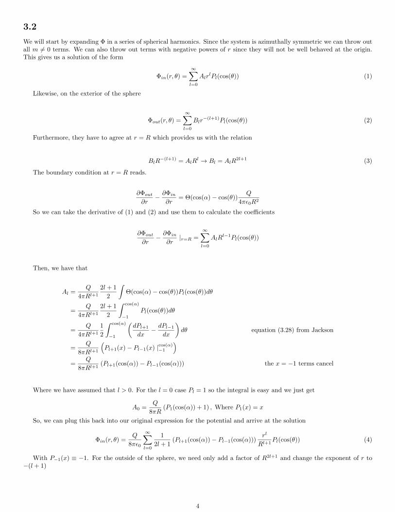
3.2

We will start by expanding Φ in a series of spherical harmonics. Since the system is azimuthally symmetric we can throw outall m 6= 0 terms. We can also throw out terms with negative powers of r since they will not be well behaved at the origin.This gives us a solution of the form

Φin(r, θ) =

∞∑l=0

AlrlPl(cos(θ)) (1)

Likewise, on the exterior of the sphere

Φout(r, θ) =

∞∑l=0

Blr−(l+1)Pl(cos(θ)) (2)

Furthermore, they have to agree at r = R which provides us with the relation

BlR−(l+1) = AlR

l → Bl = AlR2l+1 (3)

The boundary condition at r = R reads.

∂Φout∂r

− ∂Φin∂r

= Θ(cos(α)− cos(θ))Q

4πε0R2

So we can take the derivative of (1) and (2) and use them to calculate the coefficients

∂Φout∂r

− ∂Φin∂r|r=R =

∞∑l=0

AlRl−1Pl(cos(θ))

Then, we have that

Al =Q

4πRl+1

2l + 1

2

∫Θ(cos(α)− cos(θ))Pl(cos(θ))dθ

=Q

4πRl+1

2l + 1

2

∫ cos(α)

−1Pl(cos(θ))dθ

=Q

4πRl+1

1

2

∫ cos(α)

−1

(dPl+1

dx− dPl−1

dx

)dθ equation (3.28) from Jackson

=Q

8πRl+1

(Pl+1(x)− Pl−1(x) |cos(α)−1

)=

Q

8πRl+1(Pl+1(cos(α))− Pl−1(cos(α))) the x = −1 terms cancel

Where we have assumed that l > 0. For the l = 0 case Pl = 1 so the integral is easy and we just get

A0 =Q

8πR(P1(cos(α)) + 1) , Where P1(x) = x

So, we can plug this back into our original expression for the potential and arrive at the solution

Φin(r, θ) =Q

8πε0

∞∑l=0

1

2l + 1(Pl+1(cos(α))− Pl−1(cos(α)))

rl

Rl+1Pl(cos(θ)) (4)

With P−1(x) ≡ −1. For the outside of the sphere, we need only add a factor of R2l+1 and change the exponent of r to−(l + 1)

4

Φout(r, θ) =Q

8πε0

∞∑l=0

1

2l + 1(Pl+1(cos(α))− Pl−1(cos(α)))

Rl

rl+1Pl(cos(θ)) (5)

So, conveniently enough, we can just write this as

Φ(r, θ) =Q

8πε0

∞∑l=0

1

2l + 1(Pl+1(cos(α))− Pl−1(cos(α)))

rl<rl+1>

Pl(cos(θ)) (6)

where r>/< is the greater/lesser of r and R.

b.)

Well, we can start by taking the r and θ derivatives of the potential inside the sphere to get the r and θ components of theE field.

Er(r, θ) = −∂Φ

∂r= − Q

8πε0

∞∑l=1

1

2l + 1(Pl+1(cos(α))− Pl−1(cos(α)))

lrl−1

Rl+1Pl(cos(θ))

Eθ(r, θ) = −1

r

∂Φ

∂θ=

1

r

Q

8πε0

∞∑l=1

1

2l + 1(Pl+1(cos(α))− Pl−1(cos(α)))

rl

Rl+1

dPl(cos(θ))

d cos(θ)sin(θ)

Since the sitiuation is azimuthally symmetric we can just look at the x > 0 region of the x− z plane where the cartesiencomponents of the electric field are given by

Ex = sin(θ)Eρ + cos(θ)Eθ

=Q

8πε0

∞∑l=1

1

2l + 1(Pl+1(cos(α))− Pl−1(cos(α)))

rl−1

Rl+1

(dPl(cos(θ))

d cos(θ)sin(θ) cos(θ)− Pl(cos(θ)) sin(θ)

)Ez = cos(θ)Eρ − sin(θ)Eθ

= − Q

8πε0

∞∑l=1

1

2l + 1(Pl+1(cos(α))− Pl−1(cos(α)))

rl−1

Rl+1

(dPl(cos(θ))

d cos(θ)sin(θ)2 + Pl(cos(θ)) cos(θ)

)

As r → 0, only the l = 1 terms survive and these equations reduce to

Ex(r, θ) = 0

Ez(r, θ) = − Q

8πε0

1

3R2(P2(cos(α))− 1)

=Q

8πε0

1

2R2sin(α)2

Since sin(α)2 is always positive, the feld at the origin always points in the positive z direction with magntude

‖E‖ =Q

16πε0R2sin(α)2

c.)

As the cap becomes small or large we can get a good approximation by taking only the first-order taylor expansion of Pl(x)about x = ±1. This is given by

Pl(x) = Pl(±1) + (x± 1)dPldx|x=±1

5

Equation (3.28) from Jackson tells us that

dPl+1

dx− dPl+1

dx= (2l + 1)Pl

Finally, recall that Pl(1) = 1 and Pl(−1) = (−1)l. With these formulae we can reqrite Pl in terms of other legendrepolynomials. In particular, when the cap gets very small, we have that cos(α) ∼ 1 and

Φin(r, θ) ∼ Q

8πε0

∞∑l=0

1

2l + 1

(Pl+1(1) + (x− 1)

dPl+1

dx|x=1 −Pl−1(1)− (x− 1)

dPl−1dx

|x=1

)rl

Rl+1Pl(cos(θ))

=Q

8πε0

(2

R+

∞∑l=1

Pl(cos(α))(x− 1)rl

Rl+1Pl(cos(θ))

)

however (x− 1) = (cos(α)− 1) ∼ −α2

2 and Pl(cos(α)) ∼ 1 so that

Φin(r, θ) ∼ Q

4πε0R− Qα2

16πε0

∞∑l=0

rl

Rl+1Pl(cos(θ))

This is the potential of a negatively charged point particle at the point z = R with total charge proportional to α2

superimposed wth a uniform sphere of charge, perfect! For the exterior we get the same result, but with r and R swappedin the sum, exactly the expansion for a uniform sphere and point particle when r > R

Φout(r, θ) ∼Q

4πε0r− Qα2

16πε0

∞∑l=0

Rl

rl+1Pl(cos(θ))

And the electric field is obviously just that of a point particle on the interior, and a dipole on the exterior.

Now, when the cap gets very large, cos(α) ∼ −1 and we get

Φin(r, θ) ∼ Q

8πε0

∞∑l=0

1

2l + 1

(Pl+1(−1) + (x+ 1)

dPl+1

dx|x=−1 −Pl−1(−1)− (x+ 1)

dPl−1dx

|x=−1)

rl

Rl+1Pl(cos(θ))

=Q

8πε0

∞∑l=0

(x+ 1)Pl(cos(α))rl

Rl+1Pl(cos(θ))

However (x+ 1) ∼ α2

2 and Pl(cos(α)) ∼ 1 so that

Φin(r, θ) ∼ Qα2

16πε0

∞∑l=0

rl

Rl+1Pl(cos(θ))

This is the potential of a positively charged point charge at the point z = −R with total charge proportional to (π−α)2,wich is exactly the resulting charge distribution when α→ π. Again on the exterior we must only swap r and R giving

Φout(r, θ) ∼Qα2

16πε0

∞∑l=0

Rl

rl+1Pl(cos(θ))

Again, the electric field is obviously just that of a point particle.

3.6

This problem can be easily solved using the greens function approach. The charge density in spherical coordinates is givenby

ρ(x) =q

a2δ(r − a)(δ(cos(θ)− 1)− δ(cos(θ) + 1)))

The system is azimuthally symmetric, so we can expand the greens function and ignore terms with m 6= 0.

6

a.)

The azimuthally symmetric greens function expansion in free space is given by equation (3.125) in the book with a→ 0 andb→∞

G(x,x′) =

∞∑l=0

rl<rl+1>

Pl(cos(θ′))Pl(cos(θ))

The potential is given by

Φ(x) =1

4πε0

∫V

ρ(x′)

∞∑l=0

rl<rl+1>

Pl(cos(θ′))Pl(cos(θ))d3x′ (7)

For r < a we get

Φ(x) =q

4πε0

∞∑l=0

rl

al+1Pl(cos(θ))(Pl(1)− Pl(−1))

=q

2πε0

∞∑j=0

r2j−1

a2jP2j−1(cos(θ))

Where we have used the fact that Pl(1) = 1 and Pl(−1) = (−1)l. And for r > a we get

Φ(x) =q

4πε0

∞∑l=0

al

rl+1Pl(cos(θ))(Pl(1)− Pl(−1))

=q

2πε0

∞∑j=1

a2j−1

r2jP2j−1(cos(θ))

b.)

Once the limit a → 0 is taken the only sensible solution is for r > a so we use the second solution. The only term thatsurvives is the j = 1 term, since all others have at least two factors of a which causes the entire term to go to zero. Thus weget the solution

Φ(x) =p

4πε0

cos(θ)

r2=

p · z4πε0

1

r2

with p = pz, which is exactly the solution for a dipole, great!

c.)

Ok, if we are going to put this thing in a sphere, we need to use a new form of the greens function. Note that we do not needto change the solution for the potential in terms of the greens function, since the potential is zero on the surface. Really, allwe need to do is use a different form of equation (3.125) in Jackson, that is, we need to use the case where a → 0 but b iskept finite. The system is still azimuthally symmetric so we still get to throw out m 6= 0 terms. Now the greens functon isgiven by

G(x,x′) =

∞∑l=0

(rl<rl+1>

− (r>r<)l

b2l+1

)Pl(cos(θ′))Pl(cos(θ)) (8)

Of course, this (times q/4πε0) is just the potential of a point charge at x′ (along the z axis) inside the sphere, so we canjust take two of these guys and take the limit as they converge to the origin. For the dipole limit we only care about r > r′,so we get

7

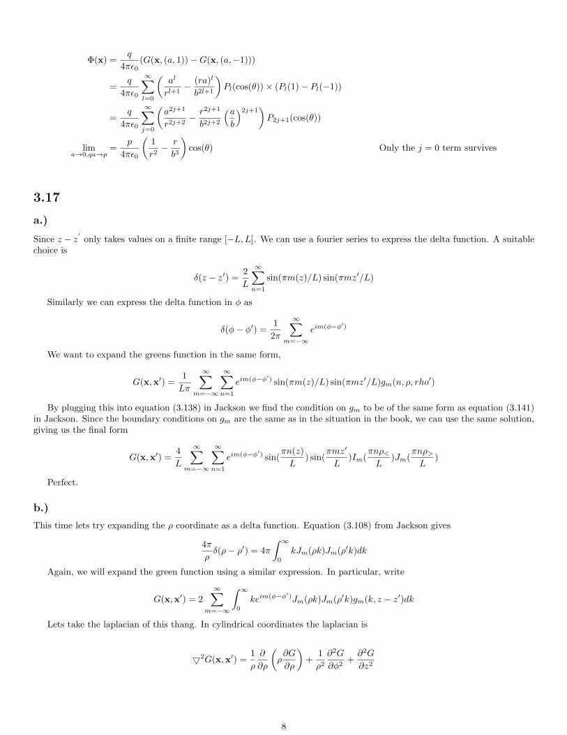
Φ(x) =q

4πε0(G(x, (a, 1))−G(x, (a,−1)))

=q

4πε0

∞∑l=0

(al

rl+1− (ra)l

b2l+1

)Pl(cos(θ))× (Pl(1)− Pl(−1))

=q

4πε0

∞∑j=0

(a2j+1

r2j+2− r2j+1

b2j+2

(ab

)2j+1)P2j+1(cos(θ))

lima→0,qa→p

=p

4πε0

(1

r2− r

b3

)cos(θ) Only the j = 0 term survives

3.17

a.)

Since z − z′ only takes values on a finite range [−L,L]. We can use a fourier series to express the delta function. A suitablechoice is

δ(z − z′) =2

L

∞∑n=1

sin(πm(z)/L) sin(πmz′/L)

Similarly we can express the delta function in φ as

δ(φ− φ′) =1

2π

∞∑m=−∞

eim(φ−φ′)

We want to expand the greens function in the same form,

G(x,x′) =1

Lπ

∞∑m=−∞

∞∑n=1

eim(φ−φ′) sin(πm(z)/L) sin(πmz′/L)gm(n, ρ, rho′)

By plugging this into equation (3.138) in Jackson we find the condition on gm to be of the same form as equation (3.141)in Jackson. Since the boundary conditions on gm are the same as in the situation in the book, we can use the same solution,giving us the final form

G(x,x′) =4

L

∞∑m=−∞

∞∑n=1

eim(φ−φ′) sin(πn(z)

L) sin(

πmz′

L)Im(

πnρ<L

)Jm(πnρ>L

)

Perfect.

b.)

This time lets try expanding the ρ coordinate as a delta function. Equation (3.108) from Jackson gives

4π

ρδ(ρ− ρ′) = 4π

∫ ∞0

kJm(ρk)Jm(ρ′k)dk

Again, we will expand the green function using a similar expression. In particular, write

G(x,x′) = 2

∞∑m=−∞

∫ ∞0

keim(φ−φ′)Jm(ρk)Jm(ρ′k)gm(k, z − z′)dk

Lets take the laplacian of this thang. In cylindrical coordinates the laplacian is

52G(x,x′) =1

ρ

∂

∂ρ

(ρ∂G

∂ρ

)+

1

ρ2∂2G

∂φ2+∂2G

∂z2

8

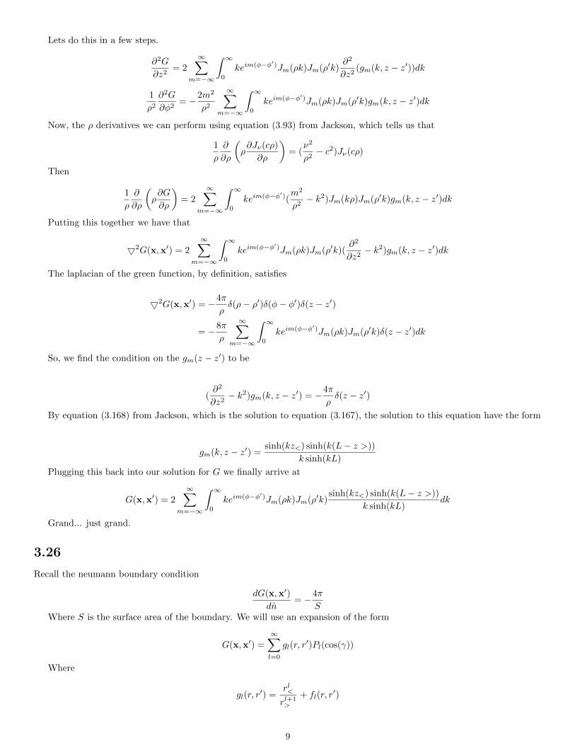
Lets do this in a few steps.

∂2G

∂z2= 2

∞∑m=−∞

∫ ∞0

keim(φ−φ′)Jm(ρk)Jm(ρ′k)∂2

∂z2(gm(k, z − z′))dk

1

ρ2∂2G

∂φ2= −2m2

ρ2

∞∑m=−∞

∫ ∞0

keim(φ−φ′)Jm(ρk)Jm(ρ′k)gm(k, z − z′)dk

Now, the ρ derivatives we can perform using equation (3.93) from Jackson, which tells us that

1

ρ

∂

∂ρ

(ρ∂Jν(cρ)

∂ρ

)= (

ν2

ρ2− c2)Jν(cρ)

Then

1

ρ

∂

∂ρ

(ρ∂G

∂ρ

)= 2

∞∑m=−∞

∫ ∞0

keim(φ−φ′)(m2

ρ2− k2)Jm(kρ)Jm(ρ′k)gm(k, z − z′)dk

Putting this together we have that

52G(x,x′) = 2

∞∑m=−∞

∫ ∞0

keim(φ−φ′)Jm(ρk)Jm(ρ′k)(∂2

∂z2− k2)gm(k, z − z′)dk

The laplacian of the green function, by definition, satisfies

52G(x,x′) = −4π

ρδ(ρ− ρ′)δ(φ− φ′)δ(z − z′)

= −8π

ρ

∞∑m=−∞

∫ ∞0

keim(φ−φ′)Jm(ρk)Jm(ρ′k)δ(z − z′)dk

So, we find the condition on the gm(z − z′) to be

(∂2

∂z2− k2)gm(k, z − z′) = −4π

ρδ(z − z′)

By equation (3.168) from Jackson, which is the solution to equation (3.167), the solution to this equation have the form

gm(k, z − z′) =sinh(kz<) sinh(k(L− z >))

k sinh(kL)

Plugging this back into our solution for G we finally arrive at

G(x,x′) = 2

∞∑m=−∞

∫ ∞0

keim(φ−φ′)Jm(ρk)Jm(ρ′k)sinh(kz<) sinh(k(L− z >))

k sinh(kL)dk

Grand... just grand.

3.26

Recall the neumann boundary condition

dG(x,x′)

dn= −4π

SWhere S is the surface area of the boundary. We will use an expansion of the form

G(x,x′) =

∞∑l=0

gl(r, r′)Pl(cos(γ))

Where

gl(r, r′) =

rl<rl+1>

+ fl(r, r′)

9

a.)

Since the neumann boundary condition requires that the derivative of the potential at the surfaces be constant, this impliesthat the derivatives of all l > 0 terms vanish at both boundaries, since these terms will still have nontrivial θ and φ dependencethrough the legendre polynomial factors. At the boundary r = a, r< = r and we get the constraint

dgldr|r=a= l

al−1

r′l+1+dfldr

= 0

or,

dfldr|r=a= −l a

l−1

r′l+1

At r = b , r = r> and we find that

−dgldr|r=b= −(l + 1)

r′l

bl+2+dfldr

= 0

or,

dfldr|r=b= (l + 1)

r′l

bl+2

Furthermore we require that the fl be functions which satisfy the homogenious form of equation (3.120). This is nessecaryin order for the greens function to still be valid. That is, for it’s laplacian to be equal to the correct combination of deltafunctions. Explicitly, we require

1

r

d2

dr2(rfl(r, r

′))− l(l + 1)

r2fl(r, r

′) = 0

The solutions to this are of the form

fl(r, r′) = Arl +Br−(l+1)

Where A and B are functions only of r′. The normal derivatives of this at r = a and r = b are

∂rfl(r, r′) |r=a = lAal−1 − (l + 1)Ba−(l+2)

∂rfl(r, r′) |r=b = lAbl−1 − (l + 1)Bb−(l+2)

Our boundary conditions then requre that

−l al−1

r′l+1= lAal−1 − (l + 1)Ba−(l+2)

(l + 1)r′l

bl+2= lAbl−1 − (l + 1)Bb−(l+2).

Ok! Now we just need to solve for A and B. These equations are just of the form

α = Aσ +Bτ

β = Aλ+Bγ

Which has the solution

A =1

σγ − τλ(γα− τβ)

B =1

σγ − τλ(σβ − λα)

10

Note that in the special case of interest here

σγ − τλ = −l(l + 1)(al−1

bl+2+bl−1

al+2)

Then we have that

A = − 1

(al−1

bl+2 − bl−1

al+2 )(al−1

bl+2

1

r′l+1+l + 1

l

r′l

(ab)l+2) (9)

B = − 1

(al−1

bl+2 − bl−1

al+2 )(r′l

al−1

bl+2+

l

l + 1

(ab)l−1

r′l+1) (10)

(11)

Which we can finally plug back into our expression for fl and simplify

fl(r, r′) =− 1

(al−1

bl+2 − bl−1

al+2 )((al−1

bl+2

1

r′l+1+l + 1

l

r′l

(ab)l+2)rl)

− 1

(al−1

bl+2 − bl−1

al+2 )((r′l

al−1

bl+2+

l

l + 1

(ab)l−1

r′l+1)r−(l+1))

=− 1

a2l+1 − b2l+1((a2l+1 1

r′l+1+l + 1

lr′l)rl)

− 1

a2l+1 − b2l+1((r′la2l+1 +

l

l + 1

(ab)2l+1

r′l+1)r−(l+1))

=1

b2l+1 − a2l+1

[l + 1

l(rr′)l +

l

l + 1

(ab)2l+1

(rr′)l+1+ a2l+1(

rl

r′l+1+

r′l

rl+1)

]

Which exactly the expression we seek! So, indeed for l > 0

gl(r, r′) =

rl<rl+1>

+1

b2l+1 − a2l+1

[l + 1

l(rr′)l +

l

l + 1

(ab)2l+1

(rr′)l+1+ a2l+1(

rl

r′l+1+

r′l

rl+1)

]

b.)

Now, the l = 0 term needs to account for the constant normal derivative at the two surfaces. Recall the neumann boundarycondition on g.

∂g

∂n(x,x′) = −4π

S, x ∈ S

Where S is the surface area of the boundary. But also

∂g

∂n(x,x′) |r=b= −

∂g

∂r(x,x′) |r=b =

1

b2− ∂f0

∂r|r=b

∂g

∂n(x,x′) |r=a=

∂g

∂r(x,x′) |r=a =

∂f0∂r|r=a

Now our conditions on f read,

df0dr|r=a= −4π

Sand

df0dr|r=b= −

1

b2+

4π

SNote that the boundary surface consists of both the sphere at r = a and r = b so the total surface area is S = 4π(a2 + b2).

Lastly note that

df0dr|r=R= B0

1

R2

Note that this is independent of A0 which tells us that A0 can be an arbitrary function of r′.

11

Now we plug this back into the above conditions on f to get

B01

a2= − 1

a2 + b2

B01

b2= − 1

b2+

1

a2 + b2

The first equation gives

B0 = − a2

a2 + b2

and the second equation agrees, so the pair indeed has a viable solution (pfew!). Finally, we can plug this stuff back into get

g0(r, r′) =1

r>−(

a2

a2 + b2

)1

r+A0(r′)

With A0(r′) and arbitrary function of r′. Now, let us plug this into equation (1.46) from the book. In order to show thatΦ is independent of the arbitrary function A0, we may focus only on the l = 0 terms and in particular on the terms involvingA0. Let us denote the sum of these terms by ΦA. These terms work out to be

ΦA =1

4πε0

∫V

ρ(x)A0(r′)P0(cos(γ))d3x +1

4π

∫S

∂Φ

∂nA0(r′)P0(cos(γ))da

Of course, ρ and the potential are related by

5 · 5(Φ) = − ρ

ε0

so we can substitute this relation in and get

Φ(x′) = − 1

4π

∫V

(5 · 5(Φ))A0(r′)d3x +1

4π

∫S

∂Φ

∂nA0(r′)da

Where we have noticed that P0 = 1. By gauss’ law this is equal to

Φ(x′) = −A0(r′)

4π

∫S

(5(Φ)) · da+A0(r′)

4π

∫S

∂Φ

∂nda

but the gradient of Φ dotted into da is just the normal derivative of Φ, so these two terms cancel, which means that allA0 dependence cancels. Pfew.

4.1

The charge distributions in these two examples are

ρa(x) =q

a2δ(r − a)δ(cos(θ))(δ(φ) + δ(φ+ π/2)− δ(φ− π/2)− δ(φ− π)

ρb(x) =q

r2δ(φ− 0)(δ(r − a)(δ(cos(θ)− 1) + δ(cos(θ) + 1))− 2δ(ρ)δ(cos(θ)− 1))

Where in the second one, the choice of φ and the choice of θ in the second term are arbitrary. Also, recall that themultipole moments are given by

qlm =

∫Y ∗lm(θ′, φ′)r′lρ(x′)d3x (12)

12

a.)

For the first charge distribution, the integral works out to simply be

qlm = qal(Y ∗lm(π

2, 0) + Y ∗lm(

π

2,−π

2)− Y ∗lm(

π

2,π

2)− Y ∗lm(

π

2, π))

= qal

√2l + 1

4π

(l −m)!

(l +m)!Pml (0)(1 + (−i)m − (i)m − (−1)m)

Note that Plm(0) = 12 (1 + (−1)l+m). Thus if m+ l is even the multipole moment is

qlm = q al

√2l + 1

4π

(l −m)!

(l +m)!(2 + 2i)

and otherwise it is zero. The first two nonzero sets of multipole moments are

({0}{

(1− i)a√

32π q, 0, (−1− i)a

√32π q} )

b.)

The second distribution has multipole moments

qlm = (Y ∗lm(0, 0)alq + Y ∗lm(π, 0′)alq)− δ0l δ0m2Y ∗00(0, 0)δ(ρ)) (13)

This works out to be

qlm = qal

√2l + 1

4π

(l −m)!

(l +m)!(Pml (1) + Pml (−1))− δ0l δ0m2q

√1

4π(14)

So, the multipole moment is just zero for l = m = 0 and otherwise is given by

qlm = qal

√2l + 1

4π

(l −m)!

(l +m)!(Pml (1) + Pml (−1)) (15)

Obviously, since it is azimuthally symmetric we could throw out the m 6= 0 terms, but whatever. The first five momentsare given by

{0}{0, 0, 0}{

0, 0, a2√

5π q, 0, 0

}{0, 0, 0, 0, 0, 0, 0}{

0, 0, 0, 0, 3a4q√π, 0, 0, 0, 0

}

c.)

Using our results from the last part, the multipole expansion of the second distribution is

Φ(x) =q

4πε0

∞∑l=1

l∑m=−l

√4π

2l + 1

(l −m)!

(l +m)!Ylm(θ, φ)

al

rl+1(Pml (1) + Pml (−1))

We also calculated the first nonzero term from the multipole expansion, which is l = 2, m = 0, and the coefficient is givenabove. Then, the lowest nonzero approximation of the potential is

Φ(x) =q

2πε0

a2

r3P2(cos(θ))

13

In the x-y plane, θ = π/2 so P2(cos(θ)) = P2(0) = −1/2 and the approximate potential, as a function of r is

Φ(x) =q

4πε0

a2

r3

The plot will be given at the end, in direct comparison with the exact potential.

d.)

Via coloumb’s law, the potential in the x-y plane is

Φ(r) =q

4πε0

(2√

r2 + a2r√

r2 + a2− 2

r

)We non-dimentionalize these formulae by pulling out a factor of q/aε0 and plot the nondimentionalized potentials as a

function of r/a. The result is

2 4 6 8 10r�a

-0.020

-0.015

-0.010

-0.005

0.005

0.010V

Figure 1: The true potential is depicted by the dotted line and the l = 2 multipole approximation by the solid line.

14