classical enumerative geometry and quantum cohomologyjmckerna/talks/enumerative.pdf · amazing...
TRANSCRIPT

Classical Enumerative Geometryand Quantum Cohomology
James McKernan
UCSB
Classical Enumerative Geometry and Quantum Cohomology – p.1

Amazing Equation
It is the purpose of this talk to convince the listener that thefollowing formula is truly amazing. end
Nd(a, b, c) =∑
d1+d2=d
a1+a2=a−1
b1+b2=b
c1+c2=c
Nd1(a1, b1, c1)Nd2
(a2, b2, c2)
[
d21d2
2
( a − 3
a1 − 1
)
− d31d2
(a − 3
a1
)
]
( b
b1
)( c
c1
)
+ 2 ·
∑
d1+d2=d
a1+a2=a
b1+b2=b−1c1+c2=c
Nd1(a1, b1, c1)Nd2
(a2, b2, c2)
[
d21d2
( a − 3
a1 − 1
)
− d31
(a − 3
a1
)
]
( b
b1 b2 1
)( c
c1
)
+ 4 ·
∑
d1+d2=d
a1+a2=a+1
b1+b2=b−2c1+c2=c
Nd1(a1, b1, c1)Nd2
(a2, b2, c2)
[
d1d2
( a − 3
a1 − 2
)
− d21
( a − 3
a1 − 1
)
]
( b
b1 b2 2
)( c
c1
)
+ 2 ·
∑
d1+d2=d
a1+a2=a+1
b1+b2=b
c1+c2=c−1
Nd1(a1, b1, c1)Nd2
(a2, b2, c2)
[
d1d2
( a − 3
a1 − 2
)
− d21
( a − 3
a1 − 1
)
]
( b
b1
)( c
c1 c2 1
)
.
Classical Enumerative Geometry and Quantum Cohomology – p.2

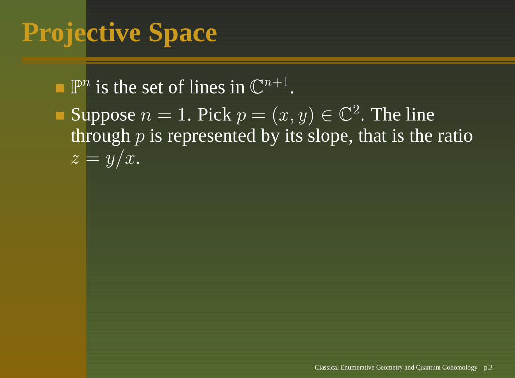
Projective Space
Pn is the set of lines in C
n+1.
Suppose n = 1. Pick p = (x, y) ∈ C2. The line
through p is represented by its slope, that is the ratioz = y/x.
We get the classical Riemann sphere, C
compactified by adding a point at infinity.
z ∈ C ∪ {∞}
Classical Enumerative Geometry and Quantum Cohomology – p.3

Automorphisms of P1
Aut(P1) = az+bcz+d
, the group of Möbiustransformations.
Suppose we are given four points p, q, r and s. Thenthere is a unique Möbius transformation, sendingp −→ 0, q −→ 1, r −→ ∞.
The image s −→ λ ∈ C − {0, 1} is called thecross-ratio.
link. In fact
λ =(r − q)(p − s)
(p − q)(r − s).
Classical Enumerative Geometry and Quantum Cohomology – p.4

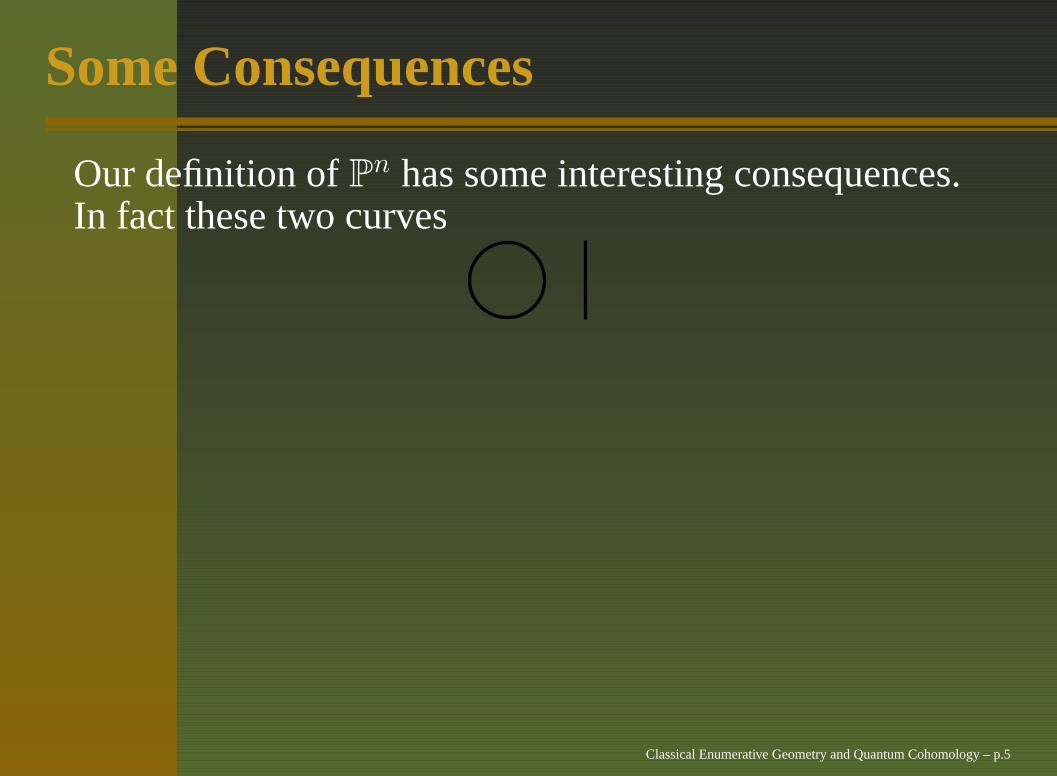
Some Consequences
Our definition of Pn has some interesting consequences.
In fact these two curves
intersect at two pointsand these two lines
meet at a point.
Principle of Continuity The number of intersection points
is an invariant of a continuous family of curves.
Classical Enumerative Geometry and Quantum Cohomology – p.5

Some Consequences
Our definition of Pn has some interesting consequences.
In fact these two curves
intersect at two points
and these two lines
meet at a point.
Principle of Continuity The number of intersection points
is an invariant of a continuous family of curves.
Classical Enumerative Geometry and Quantum Cohomology – p.5

Some Consequences
Our definition of Pn has some interesting consequences.
In fact these two curves
intersect at two pointsand these two lines
meet at a point.
Principle of Continuity The number of intersection points
is an invariant of a continuous family of curves.
Classical Enumerative Geometry and Quantum Cohomology – p.5

Some Consequences
Our definition of Pn has some interesting consequences.
In fact these two curves
intersect at two pointsand these two lines
meet at a point.
Principle of Continuity The number of intersection points
is an invariant of a continuous family of curves.Classical Enumerative Geometry and Quantum Cohomology – p.5

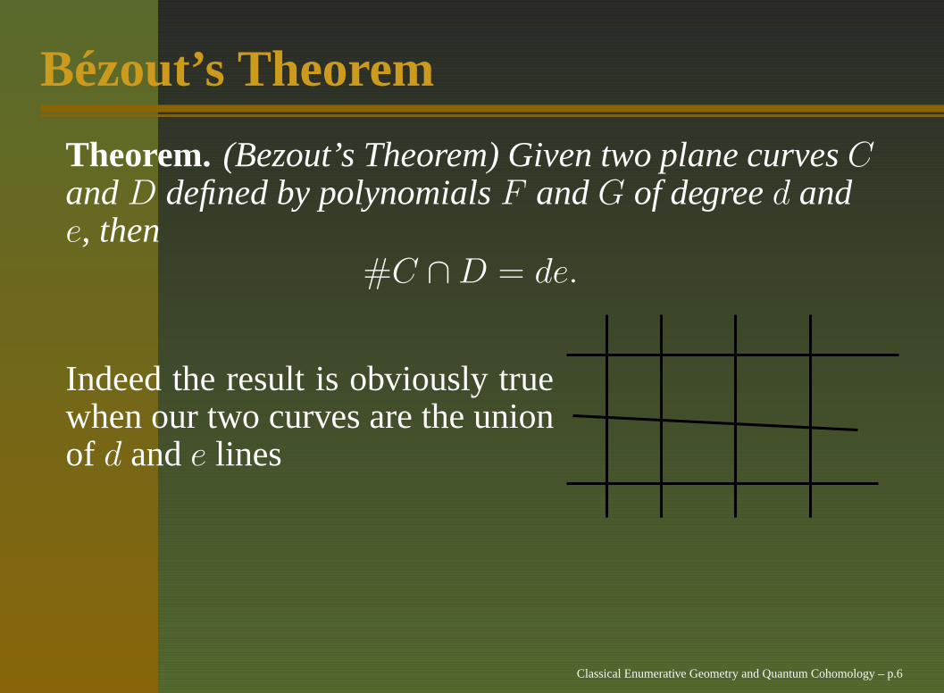
Bézout’s Theorem
Theorem. (Bezout’s Theorem) Given two plane curves Cand D defined by polynomials F and G of degree d ande, then
#C ∩ D = de.
Indeed the result is obviously truewhen our two curves are the unionof d and e lines
Proof. Let F∞ and G∞ be the product of linear forms.Then F + tF∞ and G + tG∞ define continuous familiesand when t = ∞, the answer is obviously de.
Classical Enumerative Geometry and Quantum Cohomology – p.6

The degree
The degree d of a variety Xk ⊂ Pn is the number of
points X ∩ Λ, where Λ is a general linear subspaceof dimension n − k.
Bézout’s Theorem: If we have n hypersurfacesX1, X2, . . . , Xn of degrees d1, d2, . . . , dn, then thenumber of common intersection points is
d1d2 . . . dn.
Indeed, the same proof applies.
Classical Enumerative Geometry and Quantum Cohomology – p.7

Conics in P2
A conic is given as the zero locus of
aX2 + bY 2 + cZ2 + dXY + eY Z + fXZ,
where [a : b : c : d : e : f ] ∈ P5.
How many conics pass through five points, p1, p2,p3, p4 and p5?
The condition that a conic contains a point p is alinear condition on the coefficients.
Classical Enumerative Geometry and Quantum Cohomology – p.8

Correspondence
So we have a correspondence between
{C |C contains pi } and Hi ⊂ P5,
where Hi is a hyperplane.
Thus the set of conics passing through five points,corresponds to the intersection of five hyperplanes.
So the answer is one.
Classical Enumerative Geometry and Quantum Cohomology – p.9

Correspondence
So we have a correspondence between
{C |C contains pi } and Hi ⊂ P5,
where Hi is a hyperplane.
Thus the set of conics passing through five points,corresponds to the intersection of five hyperplanes.
So the answer is one.
Classical Enumerative Geometry and Quantum Cohomology – p.9

Correspondence
So we have a correspondence between
{C |C contains pi } and Hi ⊂ P5,
where Hi is a hyperplane.
Thus the set of conics passing through five points,corresponds to the intersection of five hyperplanes.
So the answer is one.
Classical Enumerative Geometry and Quantum Cohomology – p.9

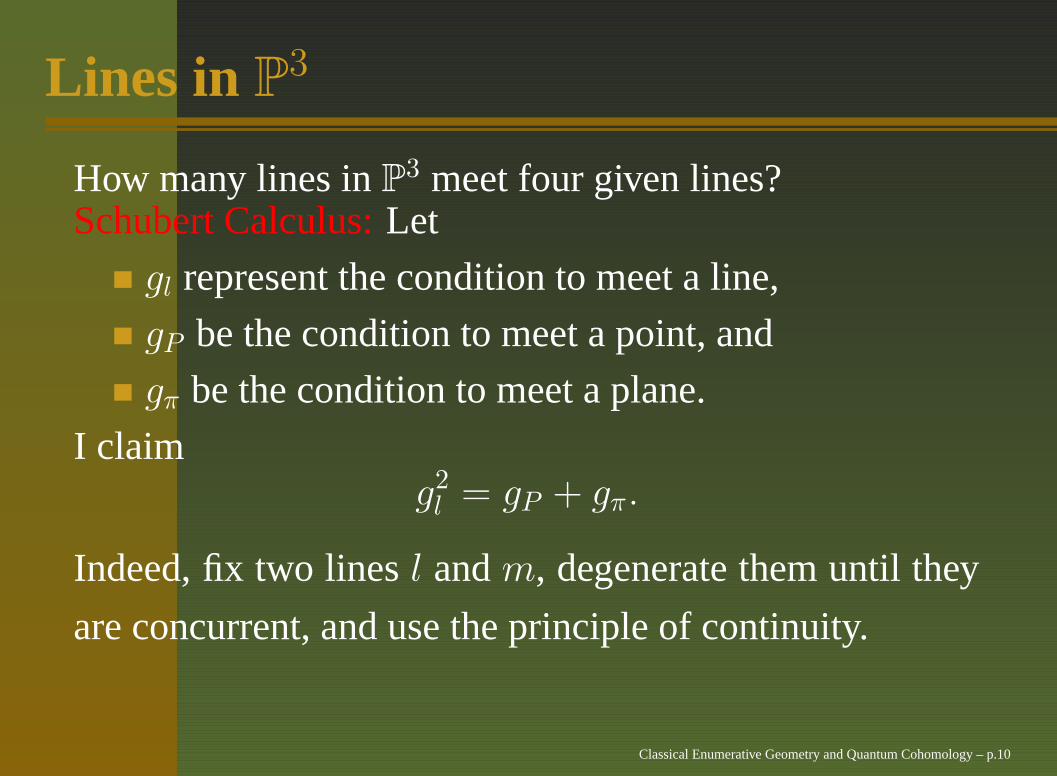
Lines in P3
How many lines in P3 meet four given lines?
Schubert Calculus: Let
gl represent the condition to meet a line,
gP be the condition to meet a point, and
gπ be the condition to meet a plane.
I claimg2
l = gP + gπ.
Indeed, fix two lines l and m, degenerate them until they
are concurrent, and use the principle of continuity.
Classical Enumerative Geometry and Quantum Cohomology – p.10
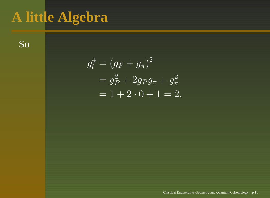
A little Algebra
So
g4
l = (gP + gπ)2
= g2
P + 2gPgπ + g2
π
= 1 + 2 · 0 + 1 = 2.
In fact we are working in the cohomology ring.
H∗(P2) =Z[x]
〈x3〉
where x is the class of a line, and C ∼ dx and D ∼ ex,so that C · D = dex2 = de.
Classical Enumerative Geometry and Quantum Cohomology – p.11

A little Algebra
So
g4
l = (gP + gπ)2
= g2
P + 2gPgπ + g2
π
= 1 + 2 · 0 + 1 = 2.
In fact we are working in the cohomology ring.
H∗(P2) =Z[x]
〈x3〉
where x is the class of a line, and C ∼ dx and D ∼ ex,so that C · D = dex2 = de.
Classical Enumerative Geometry and Quantum Cohomology – p.11

A little Algebra
So
g4
l = (gP + gπ)2
= g2
P + 2gPgπ + g2
π
= 1 + 2 · 0 + 1 = 2.
In fact we are working in the cohomology ring.
H∗(P2) =Z[x]
〈x3〉
where x is the class of a line, and C ∼ dx and D ∼ ex,so that C · D = dex2 = de.
Classical Enumerative Geometry and Quantum Cohomology – p.11

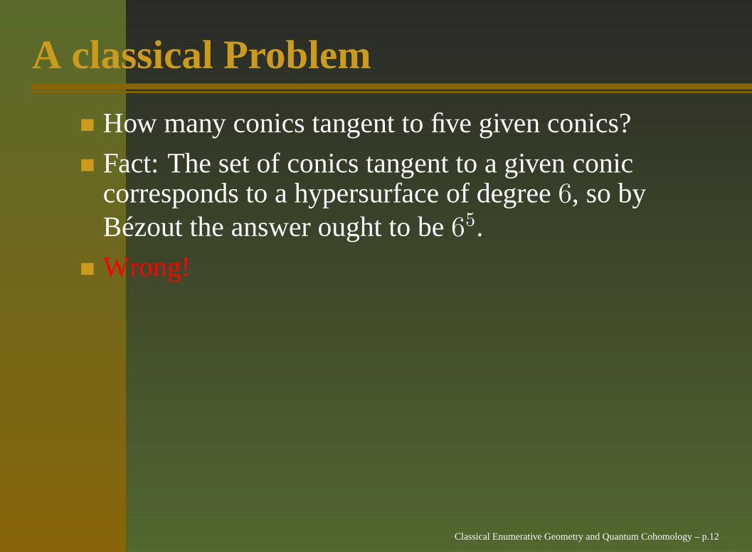
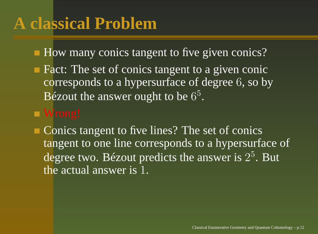
A classical Problem
How many conics tangent to five given conics?
Fact: The set of conics tangent to a given coniccorresponds to a hypersurface of degree 6, so byBézout the answer ought to be 65.
Wrong!
Conics tangent to five lines? The set of conicstangent to one line corresponds to a hypersurface ofdegree two. Bézout predicts the answer is 25. Butthe actual answer is 1.
Classical Enumerative Geometry and Quantum Cohomology – p.12
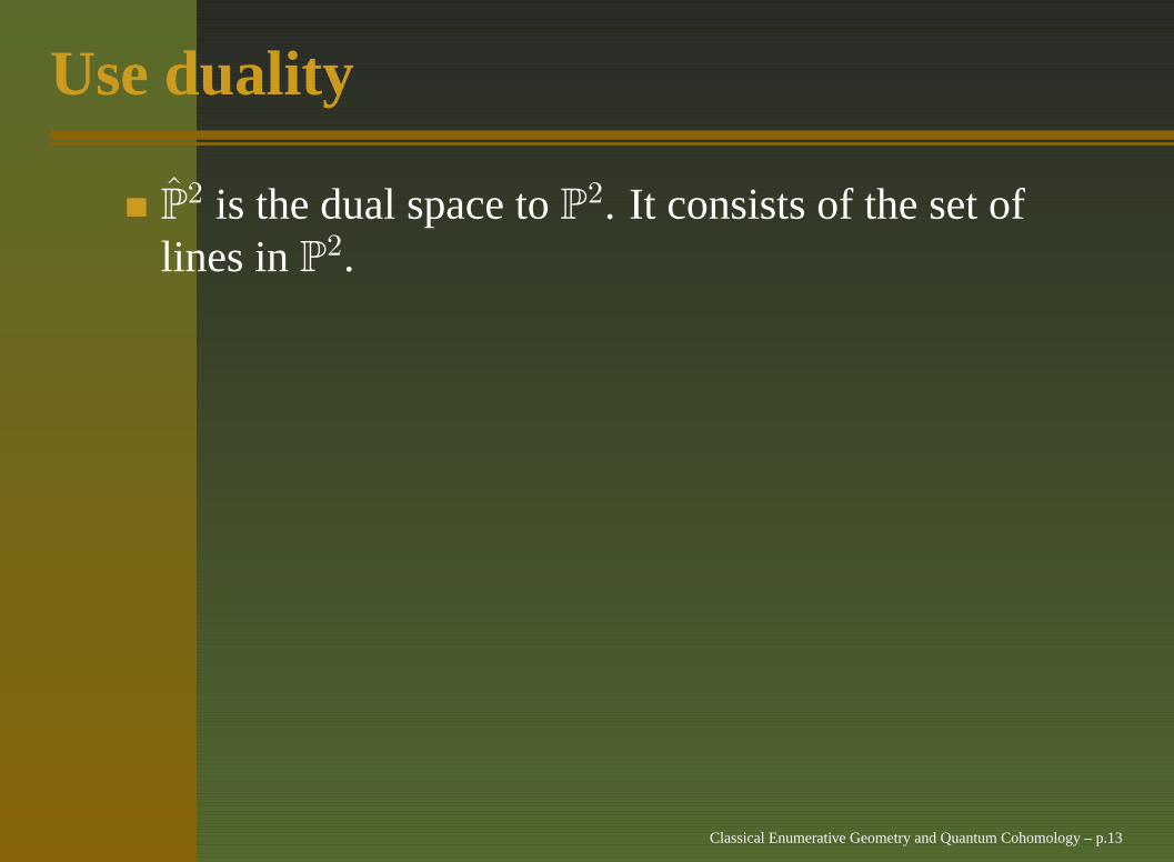
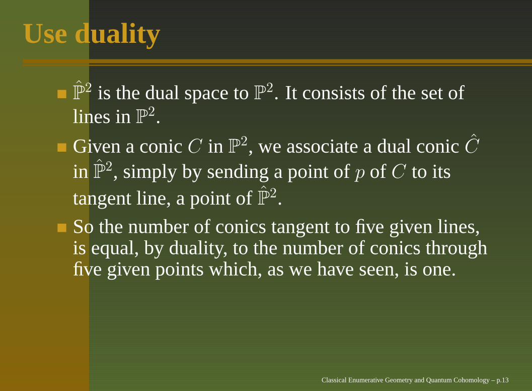
Use duality
P2 is the dual space to P
2. It consists of the set oflines in P
2.
Given a conic C in P2, we associate a dual conic C
in P2, simply by sending a point of p of C to its
tangent line, a point of P2.
So the number of conics tangent to five given lines,is equal, by duality, to the number of conics throughfive given points which, as we have seen, is one.
(Hwk) What is wrong?
Classical Enumerative Geometry and Quantum Cohomology – p.13

Physics
Here is a typical Feynmann diagram.
Feynmann diagrams are used to encode the complicated
interactions which particles undergo.
Classical Enumerative Geometry and Quantum Cohomology – p.14

String Theory
One of the ideas of string theory, is that a string is thebasic object and not particles. Replacing a point by astring, means replacing a line by a tube and ourFeynmann diagram becomes:
Classical Enumerative Geometry and Quantum Cohomology – p.15

Points at Infinity
Now take this picture and extend the tubes to infinity.Adding the points at infinity is topologically equivalentto adding caps.
p
q
r
s
Classical Enumerative Geometry and Quantum Cohomology – p.16

Back to the Riemann sphere
Topologically, the resulting surface is a sphere.
So now we have the Riemann sphere, that is a copyof P
1, with four marked points.
More generally, we will get a Riemann surface,together with a collection of marked points.
Classical Enumerative Geometry and Quantum Cohomology – p.17

Rational curves in P2
Note that plane curves of degree d correspond topolynomials of degree d, modulo scalars, which inturn corresponds to a P
N , for some N .
For example, if d = 1 we get N = 2 (in fact P2) and
if d = 2, we get N = 5, P5.
Some plane curves are rational, that is to say there isa map P
1 −→ P2, [S : T ] −→ [F : G : H], where F ,
G and H are polynomials of degree d, in S and T .
Let X ⊂ PN , be the locus of these rational curves.
Basic question: what is the degree of X ⊂ PN?
Classical Enumerative Geometry and Quantum Cohomology – p.18

The Grade
Call this degree Nd. Classically this number isknown as the grade.
N1 = 1. Indeed X1 = P2, as every line is rational.
Similarly every conic is rational, so X2 = P5 and
N2 = 1.
In general to calculate the degree of Xd we need tocut by hyperplanes. As the dimension of Xd is3d − 1, we want to cut by 3d − 1 hyperplanes.
Now imposing the condition that a curve passesthrough a point is one linear condition. So we wantto count the number of rational curves of degree dthat pass through 3d − 1 points.
Classical Enumerative Geometry and Quantum Cohomology – p.19

An argument due to Kontsevich
Fix 3d − 2 points p1, p2, . . . , p3d−2 in P2. Then we
get a 1-dimensional family of rational curves Ct ofdegree d, which contain these points.
Pick two auxiliary lines l1 and l2 and setp3d−1 = l1 ∩ l2.
Pick four points of Ct, p = p1, q = p2, r a point of l1and s a point of l2.
Observe that Ct passes through iff r = s.
Classical Enumerative Geometry and Quantum Cohomology – p.20

Picture
Here is a picture of what is going on back :
r
s
Ct
p=p1
q=p2
Classical Enumerative Geometry and Quantum Cohomology – p.21
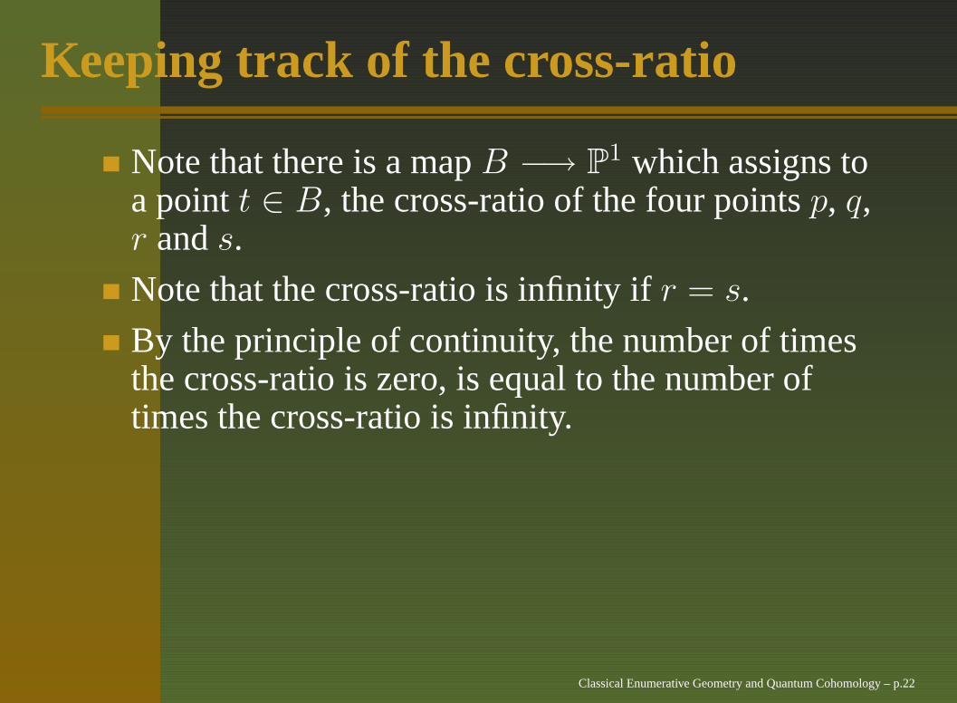
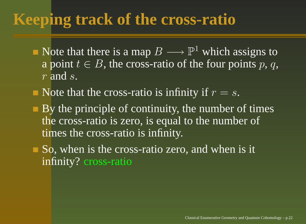
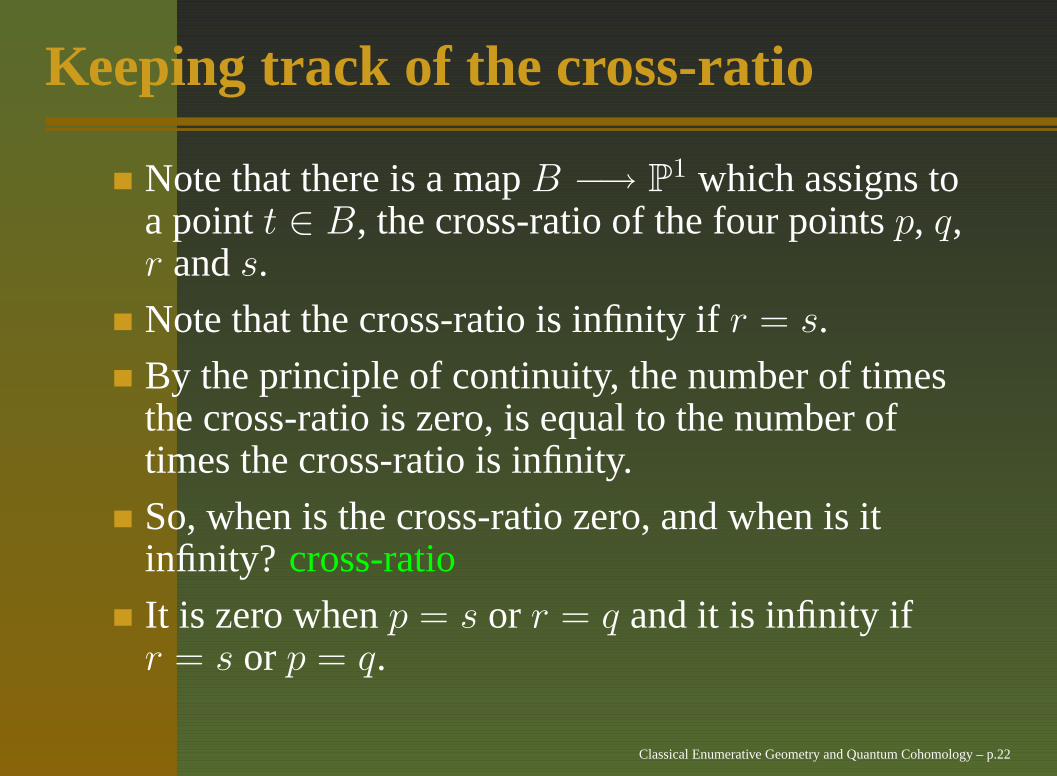
Keeping track of the cross-ratio
Note that there is a map B −→ P1 which assigns to
a point t ∈ B, the cross-ratio of the four points p, q,r and s.
Note that the cross-ratio is infinity if r = s.
By the principle of continuity, the number of timesthe cross-ratio is zero, is equal to the number oftimes the cross-ratio is infinity.
So, when is the cross-ratio zero, and when is itinfinity? cross-ratio
It is zero when p = s or r = q and it is infinity ifr = s or p = q.
Classical Enumerative Geometry and Quantum Cohomology – p.22

Picture of family Ct
pq
r
B
Classical Enumerative Geometry and Quantum Cohomology – p.23

Bubbling off
From the previous picture, it would seem that p = rand q = r can occur.
But looking at this picture, picture , in fact it wouldseem this cannot occur (and nor can p = q).
In fact what is happening, is that a copy of P1 is
bubbling off. Ct is forced to break into two curves,one of degree d1 and d2, where d = d1 + d2.
Classical Enumerative Geometry and Quantum Cohomology – p.24

Singular fibre
q
p
p
q
rs
Classical Enumerative Geometry and Quantum Cohomology – p.25

Choices
d1 and d2.
C1 passes through 3d1 − 1 points. Choose thesepoints 3d1 − 1 points, from amongst 3d − 1 − 3points.
Choose which nodes to smooth.
Choose two curves C1 and C2 through given points.
Choose the points r and s.
Classical Enumerative Geometry and Quantum Cohomology – p.26

Choices
d1 and d2.
C1 passes through 3d1 − 1 points. Choose thesepoints 3d1 − 1 points, from amongst 3d − 1 − 3points.
Choose which nodes to smooth.
Choose two curves C1 and C2 through given points.
Choose the points r and s.
Classical Enumerative Geometry and Quantum Cohomology – p.26

Choices
d1 and d2.
C1 passes through 3d1 − 1 points. Choose thesepoints 3d1 − 1 points, from amongst 3d − 1 − 3points.
Choose which nodes to smooth.
Choose two curves C1 and C2 through given points.
Choose the points r and s.
Classical Enumerative Geometry and Quantum Cohomology – p.26

Choices
d1 and d2.
C1 passes through 3d1 − 1 points. Choose thesepoints 3d1 − 1 points, from amongst 3d − 1 − 3points.
Choose which nodes to smooth.
Choose two curves C1 and C2 through given points.
Choose the points r and s.
Classical Enumerative Geometry and Quantum Cohomology – p.26

Choices
d1 and d2.
C1 passes through 3d1 − 1 points. Choose thesepoints 3d1 − 1 points, from amongst 3d − 1 − 3points.
Choose which nodes to smooth.
Choose two curves C1 and C2 through given points.
Choose the points r and s.
Classical Enumerative Geometry and Quantum Cohomology – p.26

Recursive Formula
Putting all this together we get
Nd =∑
d1+d2=d
Nd1Nd2
[
d2
1d2
2
(
3d − 4
3d1 − 1
)
− d3
1d2
(
3d − 4
3d1 − 2
)]
,
where N1 = 1 and N2 = 1.In fact N3 = 12, . . . .
Classical Enumerative Geometry and Quantum Cohomology – p.27

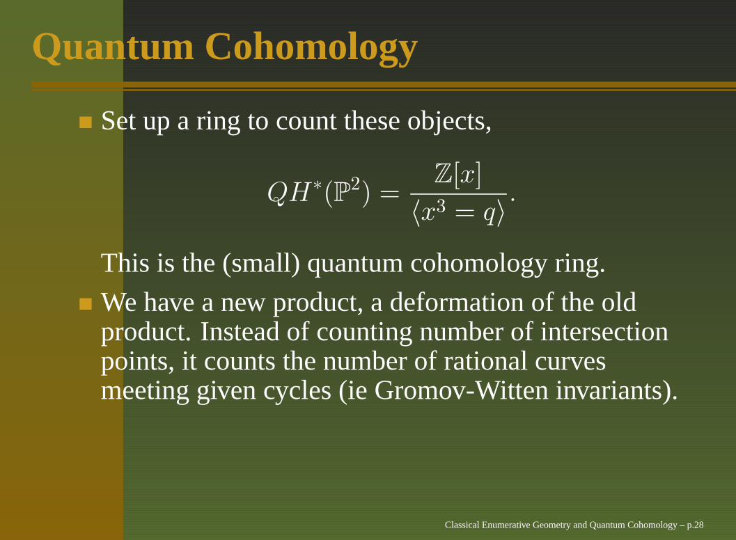
Quantum Cohomology
Set up a ring to count these objects,
QH∗(P2) =Z[x]
〈x3 = q〉.
This is the (small) quantum cohomology ring.
We have a new product, a deformation of the oldproduct. Instead of counting number of intersectionpoints, it counts the number of rational curvesmeeting given cycles (ie Gromov-Witten invariants).
Recursion formula corresponds to associativity ofquantum product.
Classical Enumerative Geometry and Quantum Cohomology – p.28

Tangency condition
For example, set Nd(a, b, c) to be the number ofcurves of degree d through a general points, tangentto b lines, and tangent to c lines, at specified generalpoints.
Formula .
In particular, we derive N2(0, 5, 0) = 3264, thecorrect answer to the question, how many conicstangent to five given lines?
Classical Enumerative Geometry and Quantum Cohomology – p.29

Further Work
Theorem. (Beauville, Yau-Zaslow) Let S be a generalK3 surface in P
g. Then the number n(g) of rationalcurves on S which are hyperplane sections is equal to
∞∑
g=1
n(g)qg =q
q∏∞
n=1(1 − qn)24
.
provided every such curve is nodal.
Theorem. (Xi Chen) Let S be a general K3 surface inP
n, such that OS(1) is not a multiple of another linebundle.Then every rational curve which is a hyperplane sectionis nodal.
Classical Enumerative Geometry and Quantum Cohomology – p.30

Further Work
Theorem. (Beauville, Yau-Zaslow) Let S be a generalK3 surface in P
g. Then the number n(g) of rationalcurves on S which are hyperplane sections is equal to
∞∑
g=1
n(g)qg =q
q∏∞
n=1(1 − qn)24
.
provided every such curve is nodal.Theorem. (Xi Chen) Let S be a general K3 surface inP
n, such that OS(1) is not a multiple of another linebundle.Then every rational curve which is a hyperplane sectionis nodal.
Classical Enumerative Geometry and Quantum Cohomology – p.30