classification: alternative techniques - gerstein lab · classification: alternative techniques...
TRANSCRIPT

5
Classification:Alternative Techniques
The previous chapter described a simple, yet quite effective, classification tech-nique known as decision tree induction. Issues such as model overfitting andclassifier evaluation were also discussed in great detail. This chapter presentsalternative techniques for building classification models—from simple tech-niques such as rule-based and nearest-neighbor classifiers to more advancedtechniques such as support vector machines and ensemble methods. Otherkey issues such as the class imbalance and multiclass problems are also dis-cussed at the end of the chapter.
5.1 Rule-Based Classifier
A rule-based classifier is a technique for classifying records using a collectionof “if . . .then. . .” rules. Table 5.1 shows an example of a model generated by arule-based classifier for the vertebrate classification problem. The rules for themodel are represented in a disjunctive normal form, R = (r1∨r2∨. . . rk), whereR is known as the rule set and ri’s are the classification rules or disjuncts.
Table 5.1. Example of a rule set for the vertebrate classification problem.
r1: (Gives Birth = no) ∧ (Aerial Creature = yes) −→ Birdsr2: (Gives Birth = no) ∧ (Aquatic Creature = yes) −→ Fishesr3: (Gives Birth = yes) ∧ (Body Temperature = warm-blooded) −→ Mammalsr4: (Gives Birth = no) ∧ (Aerial Creature = no) −→ Reptilesr5: (Aquatic Creature = semi) −→ Amphibians

208 Chapter 5 Classification: Alternative Techniques
Each classification rule can be expressed in the following way:
ri : (Conditioni) −→ yi. (5.1)
The left-hand side of the rule is called the rule antecedent or precondition.It contains a conjunction of attribute tests:
Conditioni = (A1 op v1) ∧ (A2 op v2) ∧ . . . (Ak op vk), (5.2)
where (Aj , vj) is an attribute-value pair and op is a logical operator chosenfrom the set {=, 6=, <, >,≤,≥}. Each attribute test (Aj op vj) is known asa conjunct. The right-hand side of the rule is called the rule consequent,which contains the predicted class yi.
A rule r covers a record x if the precondition of r matches the attributesof x. r is also said to be fired or triggered whenever it covers a given record.For an illustration, consider the rule r1 given in Table 5.1 and the followingattributes for two vertebrates: hawk and grizzly bear.
Name Body Skin Gives Aquatic Aerial Has Hiber-Temperature Cover Birth Creature Creature Legs nates
hawk warm-blooded feather no no yes yes nogrizzly bear warm-blooded fur yes no no yes yes
r1 covers the first vertebrate because its precondition is satisfied by the hawk’sattributes. The rule does not cover the second vertebrate because grizzly bearsgive birth to their young and cannot fly, thus violating the precondition of r1.
The quality of a classification rule can be evaluated using measures such ascoverage and accuracy. Given a data set D and a classification rule r : A −→ y,the coverage of the rule is defined as the fraction of records in D that triggerthe rule r. On the other hand, its accuracy or confidence factor is defined asthe fraction of records triggered by r whose class labels are equal to y. Theformal definitions of these measures are
Coverage(r) =|A||D|
Accuracy(r) =|A ∩ y||A| , (5.3)
where |A| is the number of records that satisfy the rule antecedent, |A ∩ y| isthe number of records that satisfy both the antecedent and consequent, and|D| is the total number of records.

5.1 Rule-Based Classifier 209
Table 5.2. The vertebrate data set.
Name Body Skin Gives Aquatic Aerial Has Hiber- Class LabelTemperature Cover Birth Creature Creature Legs nates
human warm-blooded hair yes no no yes no Mammalspython cold-blooded scales no no no no yes Reptilessalmon cold-blooded scales no yes no no no Fisheswhale warm-blooded hair yes yes no no no Mammalsfrog cold-blooded none no semi no yes yes Amphibianskomododragon
cold-blooded scales no no no yes no Reptiles
bat warm-blooded hair yes no yes yes yes Mammalspigeon warm-blooded feathers no no yes yes no Birdscat warm-blooded fur yes no no yes no Mammalsguppy cold-blooded scales yes yes no no no Fishesalligator cold-blooded scales no semi no yes no Reptilespenguin warm-blooded feathers no semi no yes no Birdsporcupine warm-blooded quills yes no no yes yes Mammalseel cold-blooded scales no yes no no no Fishessalamander cold-blooded none no semi no yes yes Amphibians
Example 5.1. Consider the data set shown in Table 5.2. The rule
(Gives Birth = yes) ∧ (Body Temperature = warm-blooded) −→ Mammals
has a coverage of 33% since five of the fifteen records support the rule an-tecedent. The rule accuracy is 100% because all five vertebrates covered bythe rule are mammals.
5.1.1 How a Rule-Based Classifier Works
A rule-based classifier classifies a test record based on the rule triggered bythe record. To illustrate how a rule-based classifier works, consider the ruleset shown in Table 5.1 and the following vertebrates:
Name Body Skin Gives Aquatic Aerial Has Hiber-Temperature Cover Birth Creature Creature Legs nates
lemur warm-blooded fur yes no no yes yesturtle cold-blooded scales no semi no yes nodogfish shark cold-blooded scales yes yes no no no
• The first vertebrate, which is a lemur, is warm-blooded and gives birthto its young. It triggers the rule r3, and thus, is classified as a mammal.

210 Chapter 5 Classification: Alternative Techniques
• The second vertebrate, which is a turtle, triggers the rules r4 and r5.Since the classes predicted by the rules are contradictory (reptiles versusamphibians), their conflicting classes must be resolved.
• None of the rules are applicable to a dogfish shark. In this case, weneed to ensure that the classifier can still make a reliable prediction eventhough a test record is not covered by any rule.
The previous example illustrates two important properties of the rule set gen-erated by a rule-based classifier.
Mutually Exclusive Rules The rules in a rule set R are mutually exclusiveif no two rules in R are triggered by the same record. This property ensuresthat every record is covered by at most one rule in R. An example of amutually exclusive rule set is shown in Table 5.3.
Exhaustive Rules A rule set R has exhaustive coverage if there is a rulefor each combination of attribute values. This property ensures that everyrecord is covered by at least one rule in R. Assuming that Body Temperature
and Gives Birth are binary variables, the rule set shown in Table 5.3 hasexhaustive coverage.
Table 5.3. Example of a mutually exclusive and exhaustive rule set.
r1: (Body Temperature = cold-blooded) −→ Non-mammalsr2: (Body Temperature = warm-blooded) ∧ (Gives Birth = yes) −→ Mammalsr3: (Body Temperature = warm-blooded) ∧ (Gives Birth = no) −→ Non-mammals
Together, these properties ensure that every record is covered by exactlyone rule. Unfortunately, many rule-based classifiers, including the one shownin Table 5.1, do not have such properties. If the rule set is not exhaustive,then a default rule, rd : () −→ yd, must be added to cover the remainingcases. A default rule has an empty antecedent and is triggered when all otherrules have failed. yd is known as the default class and is typically assigned tothe majority class of training records not covered by the existing rules.
If the rule set is not mutually exclusive, then a record can be covered byseveral rules, some of which may predict conflicting classes. There are twoways to overcome this problem.

5.1 Rule-Based Classifier 211
Ordered Rules In this approach, the rules in a rule set are ordered indecreasing order of their priority, which can be defined in many ways (e.g.,based on accuracy, coverage, total description length, or the order in whichthe rules are generated). An ordered rule set is also known as a decisionlist. When a test record is presented, it is classified by the highest-ranked rulethat covers the record. This avoids the problem of having conflicting classespredicted by multiple classification rules.
Unordered Rules This approach allows a test record to trigger multipleclassification rules and considers the consequent of each rule as a vote fora particular class. The votes are then tallied to determine the class labelof the test record. The record is usually assigned to the class that receivesthe highest number of votes. In some cases, the vote may be weighted bythe rule’s accuracy. Using unordered rules to build a rule-based classifier hasboth advantages and disadvantages. Unordered rules are less susceptible toerrors caused by the wrong rule being selected to classify a test record (unlikeclassifiers based on ordered rules, which are sensitive to the choice of rule-ordering criteria). Model building is also less expensive because the rules donot have to be kept in sorted order. Nevertheless, classifying a test record canbe quite an expensive task because the attributes of the test record must becompared against the precondition of every rule in the rule set.
In the remainder of this section, we will focus on rule-based classifiers thatuse ordered rules.
5.1.2 Rule-Ordering Schemes
Rule ordering can be implemented on a rule-by-rule basis or on a class-by-classbasis. The difference between these schemes is illustrated in Figure 5.1.
Rule-Based Ordering Scheme This approach orders the individual rulesby some rule quality measure. This ordering scheme ensures that every testrecord is classified by the “best” rule covering it. A potential drawback of thisscheme is that lower-ranked rules are much harder to interpret because theyassume the negation of the rules preceding them. For example, the fourth ruleshown in Figure 5.1 for rule-based ordering,
Aquatic Creature = semi −→ Amphibians,
has the following interpretation: If the vertebrate does not have any feathersor cannot fly, and is cold-blooded and semi-aquatic, then it is an amphibian.

212 Chapter 5 Classification: Alternative Techniques
(Skin Cover=feathers, Aerial Creature=yes) ==> Birds
(Skin Cover=scales, Aquatic Creature=no) ==> Reptiles
(Skin Cover=scales, Aquatic Creature=yes) ==> Fishes
(Skin Cover=none) ==> Amphibians
(Body temperature=warm-blooded,Gives Birth=yes) ==> Mammals
(Body temperature=warm-blooded,Gives Birth=no) ==> Birds
(Aquatic Creature=semi)) ==> Amphibians
Rule-Based Ordering
(Skin Cover=feathers, Aerial Creature=yes) ==> Birds
(Skin Cover=scales, Aquatic Creature=no) ==> Reptiles
(Skin Cover=scales, Aquatic Creature=yes) ==> Fishes
(Skin Cover=none) ==> Amphibians
(Body temperature=warm-blooded,Gives Birth=yes) ==> Mammals
(Body temperature=warm-blooded,Gives Birth=no) ==> Birds
(Aquatic Creature=semi)) ==> Amphibians
Class-Based Ordering
Figure 5.1. Comparison between rule-based and class-based ordering schemes.
The additional conditions (that the vertebrate does not have any feathers orcannot fly, and is cold-blooded) are due to the fact that the vertebrate doesnot satisfy the first three rules. If the number of rules is large, interpreting themeaning of the rules residing near the bottom of the list can be a cumbersometask.
Class-Based Ordering Scheme In this approach, rules that belong to thesame class appear together in the rule set R. The rules are then collectivelysorted on the basis of their class information. The relative ordering among therules from the same class is not important; as long as one of the rules fires,the class will be assigned to the test record. This makes rule interpretationslightly easier. However, it is possible for a high-quality rule to be overlookedin favor of an inferior rule that happens to predict the higher-ranked class.
Since most of the well-known rule-based classifiers (such as C4.5rules andRIPPER) employ the class-based ordering scheme, the discussion in the re-mainder of this section focuses mainly on this type of ordering scheme.
5.1.3 How to Build a Rule-Based Classifier
To build a rule-based classifier, we need to extract a set of rules that identifieskey relationships between the attributes of a data set and the class label.

5.1 Rule-Based Classifier 213
There are two broad classes of methods for extracting classification rules: (1)direct methods, which extract classification rules directly from data, and (2)indirect methods, which extract classification rules from other classificationmodels, such as decision trees and neural networks.
Direct methods partition the attribute space into smaller subspaces so thatall the records that belong to a subspace can be classified using a single classi-fication rule. Indirect methods use the classification rules to provide a succinctdescription of more complex classification models. Detailed discussions of thesemethods are presented in Sections 5.1.4 and 5.1.5, respectively.
5.1.4 Direct Methods for Rule Extraction
The sequential covering algorithm is often used to extract rules directlyfrom data. Rules are grown in a greedy fashion based on a certain evaluationmeasure. The algorithm extracts the rules one class at a time for data setsthat contain more than two classes. For the vertebrate classification problem,the sequential covering algorithm may generate rules for classifying birds first,followed by rules for classifying mammals, amphibians, reptiles, and finally,fishes (see Figure 5.1). The criterion for deciding which class should be gen-erated first depends on a number of factors, such as the class prevalence (i.e.,fraction of training records that belong to a particular class) or the cost ofmisclassifying records from a given class.
A summary of the sequential covering algorithm is given in Algorithm5.1. The algorithm starts with an empty decision list, R. The Learn-One-Rule function is then used to extract the best rule for class y that covers thecurrent set of training records. During rule extraction, all training recordsfor class y are considered to be positive examples, while those that belong to
Algorithm 5.1 Sequential covering algorithm.
1: Let E be the training records and A be the set of attribute-value pairs, {(Aj , vj)}.2: Let Yo be an ordered set of classes {y1, y2, . . . , yk}.3: Let R = { } be the initial rule list.4: for each class y ∈ Yo − {yk} do5: while stopping condition is not met do6: r ← Learn-One-Rule (E, A, y).7: Remove training records from E that are covered by r.8: Add r to the bottom of the rule list: R −→ R ∨ r.9: end while
10: end for11: Insert the default rule, {} −→ yk, to the bottom of the rule list R.

214 Chapter 5 Classification: Alternative Techniques
other classes are considered to be negative examples. A rule is desirable if itcovers most of the positive examples and none (or very few) of the negativeexamples. Once such a rule is found, the training records covered by the ruleare eliminated. The new rule is added to the bottom of the decision list R.This procedure is repeated until the stopping criterion is met. The algorithmthen proceeds to generate rules for the next class.
Figure 5.2 demonstrates how the sequential covering algorithm works fora data set that contains a collection of positive and negative examples. Therule R1, whose coverage is shown in Figure 5.2(b), is extracted first becauseit covers the largest fraction of positive examples. All the training recordscovered by R1 are subsequently removed and the algorithm proceeds to lookfor the next best rule, which is R2.
R1
R1
R1
R2
(a) Original Data (b) Step 1
(c) Step 2 (d) Step 3
Figure 5.2. An example of the sequential covering algorithm.

5.1 Rule-Based Classifier 215
Learn-One-Rule Function
The objective of the Learn-One-Rule function is to extract a classificationrule that covers many of the positive examples and none (or very few) of thenegative examples in the training set. However, finding an optimal rule iscomputationally expensive given the exponential size of the search space. TheLearn-One-Rule function addresses the exponential search problem by growingthe rules in a greedy fashion. It generates an initial rule r and keeps refiningthe rule until a certain stopping criterion is met. The rule is then pruned toimprove its generalization error.
Rule-Growing Strategy There are two common strategies for growing aclassification rule: general-to-specific or specific-to-general. Under the general-to-specific strategy, an initial rule r : {} −→ y is created, where the left-handside is an empty set and the right-hand side contains the target class. The rulehas poor quality because it covers all the examples in the training set. New
Body Temperature = warm-blooded, Has Legs = yes => Mammals
Body Temperature=warm-blooded, Skin Cover=hair, Gives Birth=yes, Aquatic creature=no, Aerial Creature=no
Has Legs=yes, Hibernates=no => Mammals
Body Temperature=warm-blooded, Skin Cover=hair, Gives Birth=yes,
Aquatic creature=no, Aerial Creature=no Has Legs=yes => Mammals
Skin Cover = hair => Mammals
{ } => Mammals
Body Temperature = warm-blooded => Mammals
Body Temperature = warm-blooded, Gives Birth = yes => Mammals
Has Legs = No => Mammals
(a) General-to-specific
(b) Specific-to-general
. . .
. . .
. . .
Skin Cover=hair, Gives Birth=yes Aquatic Creature=no, Aerial Creature=no,
Has Legs=yes, Hibernates=no => Mammals
Figure 5.3. General-to-specific and specific-to-general rule-growing strategies.

216 Chapter 5 Classification: Alternative Techniques
conjuncts are subsequently added to improve the rule’s quality. Figure 5.3(a)shows the general-to-specific rule-growing strategy for the vertebrate classifi-cation problem. The conjunct Body Temperature=warm-blooded is initiallychosen to form the rule antecedent. The algorithm then explores all the possi-ble candidates and greedily chooses the next conjunct, Gives Birth=yes, tobe added into the rule antecedent. This process continues until the stoppingcriterion is met (e.g., when the added conjunct does not improve the qualityof the rule).
For the specific-to-general strategy, one of the positive examples is ran-domly chosen as the initial seed for the rule-growing process. During therefinement step, the rule is generalized by removing one of its conjuncts sothat it can cover more positive examples. Figure 5.3(b) shows the specific-to-general approach for the vertebrate classification problem. Suppose a positiveexample for mammals is chosen as the initial seed. The initial rule containsthe same conjuncts as the attribute values of the seed. To improve its cov-erage, the rule is generalized by removing the conjunct Hibernate=no. Therefinement step is repeated until the stopping criterion is met, e.g., when therule starts covering negative examples.
The previous approaches may produce suboptimal rules because the rulesare grown in a greedy fashion. To avoid this problem, a beam search may beused, where k of the best candidate rules are maintained by the algorithm.Each candidate rule is then grown separately by adding (or removing) a con-junct from its antecedent. The quality of the candidates are evaluated and thek best candidates are chosen for the next iteration.
Rule Evaluation An evaluation metric is needed to determine which con-junct should be added (or removed) during the rule-growing process. Accu-racy is an obvious choice because it explicitly measures the fraction of trainingexamples classified correctly by the rule. However, a potential limitation of ac-curacy is that it does not take into account the rule’s coverage. For example,consider a training set that contains 60 positive examples and 100 negativeexamples. Suppose we are given the following two candidate rules:
Rule r1: covers 50 positive examples and 5 negative examples,Rule r2: covers 2 positive examples and no negative examples.
The accuracies for r1 and r2 are 90.9% and 100%, respectively. However,r1 is the better rule despite its lower accuracy. The high accuracy for r2 ispotentially spurious because the coverage of the rule is too low.

5.1 Rule-Based Classifier 217
The following approaches can be used to handle this problem.
1. A statistical test can be used to prune rules that have poor coverage.For example, we may compute the following likelihood ratio statistic:
R = 2
k∑
i=1
fi log(fi/ei),
where k is the number of classes, fi is the observed frequency of class iexamples that are covered by the rule, and ei is the expected frequencyof a rule that makes random predictions. Note that R has a chi-squaredistribution with k − 1 degrees of freedom. A large R value suggeststhat the number of correct predictions made by the rule is significantlylarger than that expected by random guessing. For example, since r1
covers 55 examples, the expected frequency for the positive class is e+ =55×60/160 = 20.625, while the expected frequency for the negative classis e− = 55× 100/160 = 34.375. Thus, the likelihood ratio for r1 is
R(r1) = 2× [50× log2(50/20.625) + 5× log2(5/34.375)] = 99.9.
Similarly, the expected frequencies for r2 are e+ = 2 × 60/160 = 0.75and e− = 2× 100/160 = 1.25. The likelihood ratio statistic for r2 is
R(r2) = 2× [2× log2(2/0.75) + 0× log2(0/1.25)] = 5.66.
This statistic therefore suggests that r1 is a better rule than r2.
2. An evaluation metric that takes into account the rule coverage can beused. Consider the following evaluation metrics:
Laplace =f+ + 1
n + k, (5.4)
m-estimate =f+ + kp+
n + k, (5.5)
where n is the number of examples covered by the rule, f+ is the numberof positive examples covered by the rule, k is the total number of classes,and p+ is the prior probability for the positive class. Note that the m-estimate is equivalent to the Laplace measure by choosing p+ = 1/k.Depending on the rule coverage, these measures capture the trade-off

218 Chapter 5 Classification: Alternative Techniques
between rule accuracy and the prior probability of the positive class. Ifthe rule does not cover any training example, then the Laplace mea-sure reduces to 1/k, which is the prior probability of the positive classassuming a uniform class distribution. The m-estimate also reduces tothe prior probability (p+) when n = 0. However, if the rule coverageis large, then both measures asymptotically approach the rule accuracy,f+/n. Going back to the previous example, the Laplace measure forr1 is 51/57 = 89.47%, which is quite close to its accuracy. Conversely,the Laplace measure for r2 (75%) is significantly lower than its accuracybecause r2 has a much lower coverage.
3. An evaluation metric that takes into account the support count of therule can be used. One such metric is the FOIL’s information gain.The support count of a rule corresponds to the number of positive exam-ples covered by the rule. Suppose the rule r : A −→ + covers p0 positiveexamples and n0 negative examples. After adding a new conjunct B, theextended rule r′ : A∧B −→ + covers p1 positive examples and n1 neg-ative examples. Given this information, the FOIL’s information gain ofthe extended rule is defined as follows:
FOIL’s information gain = p1 ×(
log2
p1
p1 + n1− log2
p0
p0 + n0
). (5.6)
Since the measure is proportional to p1 and p1/(p1 +n1), it prefers rulesthat have high support count and accuracy. The FOIL’s informationgains for rules r1 and r2 given in the preceding example are 43.12 and 2,respectively. Therefore, r1 is a better rule than r2.
Rule Pruning The rules generated by the Learn-One-Rule function can bepruned to improve their generalization errors. To determine whether pruningis necessary, we may apply the methods described in Section 4.4 on page172 to estimate the generalization error of a rule. For example, if the erroron validation set decreases after pruning, we should keep the simplified rule.Another approach is to compare the pessimistic error of the rule before andafter pruning (see Section 4.4.4 on page 179). The simplified rule is retainedin place of the original rule if the pessimistic error improves after pruning.

5.1 Rule-Based Classifier 219
Rationale for Sequential Covering
After a rule is extracted, the sequential covering algorithm must eliminateall the positive and negative examples covered by the rule. The rationale fordoing this is given in the next example.
class = +
class = -
+
+
+++++ +
+++
++
+
+ + + + +
++
+
+
++
++
+ +
--
-
--
-
-
-
- --
--
- ---
-
- -
-
R1
R3 R2
Figure 5.4. Elimination of training records by the sequential covering algorithm. R1, R2, and R3
represent regions covered by three different rules.
Figure 5.4 shows three possible rules, R1, R2, and R3, extracted from adata set that contains 29 positive examples and 21 negative examples. Theaccuracies of R1, R2, and R3 are 12/15 (80%), 7/10 (70%), and 8/12 (66.7%),respectively. R1 is generated first because it has the highest accuracy. Aftergenerating R1, it is clear that the positive examples covered by the rule must beremoved so that the next rule generated by the algorithm is different than R1.Next, suppose the algorithm is given the choice of generating either R2 or R3.Even though R2 has higher accuracy than R3, R1 and R3 together cover 18positive examples and 5 negative examples (resulting in an overall accuracy of78.3%), whereas R1 and R2 together cover 19 positive examples and 6 negativeexamples (resulting in an overall accuracy of 76%). The incremental impact ofR2 or R3 on accuracy is more evident when the positive and negative examplescovered by R1 are removed before computing their accuracies. In particular, ifpositive examples covered by R1 are not removed, then we may overestimatethe effective accuracy of R3, and if negative examples are not removed, thenwe may underestimate the accuracy of R3. In the latter case, we might end uppreferring R2 over R3 even though half of the false positive errors committedby R3 have already been accounted for by the preceding rule, R1.

220 Chapter 5 Classification: Alternative Techniques
RIPPER Algorithm
To illustrate the direct method, we consider a widely used rule induction algo-rithm called RIPPER. This algorithm scales almost linearly with the numberof training examples and is particularly suited for building models from datasets with imbalanced class distributions. RIPPER also works well with noisydata sets because it uses a validation set to prevent model overfitting.
For two-class problems, RIPPER chooses the majority class as its defaultclass and learns the rules for detecting the minority class. For multiclass prob-lems, the classes are ordered according to their frequencies. Let (y1, y2, . . . , yc)be the ordered classes, where y1 is the least frequent class and yc is the mostfrequent class. During the first iteration, instances that belong to y1 are la-beled as positive examples, while those that belong to other classes are labeledas negative examples. The sequential covering method is used to generate rulesthat discriminate between the positive and negative examples. Next, RIPPERextracts rules that distinguish y2 from other remaining classes. This processis repeated until we are left with yc, which is designated as the default class.
Rule Growing RIPPER employs a general-to-specific strategy to grow arule and the FOIL’s information gain measure to choose the best conjunctto be added into the rule antecedent. It stops adding conjuncts when therule starts covering negative examples. The new rule is then pruned basedon its performance on the validation set. The following metric is computed todetermine whether pruning is needed: (p−n)/(p+n), where p (n) is the numberof positive (negative) examples in the validation set covered by the rule. Thismetric is monotonically related to the rule’s accuracy on the validation set. Ifthe metric improves after pruning, then the conjunct is removed. Pruning isdone starting from the last conjunct added to the rule. For example, given arule ABCD −→ y, RIPPER checks whether D should be pruned first, followedby CD, BCD, etc. While the original rule covers only positive examples, thepruned rule may cover some of the negative examples in the training set.
Building the Rule Set After generating a rule, all the positive and negativeexamples covered by the rule are eliminated. The rule is then added into therule set as long as it does not violate the stopping condition, which is basedon the minimum description length principle. If the new rule increases thetotal description length of the rule set by at least d bits, then RIPPER stopsadding rules into its rule set (by default, d is chosen to be 64 bits). Anotherstopping condition used by RIPPER is that the error rate of the rule on thevalidation set must not exceed 50%.

5.1 Rule-Based Classifier 221
RIPPER also performs additional optimization steps to determine whethersome of the existing rules in the rule set can be replaced by better alternativerules. Readers who are interested in the details of the optimization methodmay refer to the reference cited at the end of this chapter.
5.1.5 Indirect Methods for Rule Extraction
This section presents a method for generating a rule set from a decision tree.In principle, every path from the root node to the leaf node of a decision treecan be expressed as a classification rule. The test conditions encountered alongthe path form the conjuncts of the rule antecedent, while the class label at theleaf node is assigned to the rule consequent. Figure 5.5 shows an example of arule set generated from a decision tree. Notice that the rule set is exhaustiveand contains mutually exclusive rules. However, some of the rules can besimplified as shown in the next example.
No Yes
No NoYes Yes
No Yes
P
Q
Q
R
- + +
- +
r1: (P=No,Q=No) ==> -
r2: (P=No,Q=Yes) ==> +
r3: (P=Yes,Q=No) ==> +
r4: (P=Yes,R=Yes,Q=No) ==> -
r5: (P=Yes,R=Yes,Q=Yes) ==> +
Rule Set
Figure 5.5. Converting a decision tree into classification rules.
Example 5.2. Consider the following three rules from Figure 5.5:
r2 : (P = No) ∧ (Q = Yes) −→ +r3 : (P = Yes) ∧ (R = No) −→ +r5 : (P = Yes) ∧ (R = Yes) ∧ (Q = Yes) −→ +
Observe that the rule set always predicts a positive class when the value of Qis Yes. Therefore, we may simplify the rules as follows:
r2′: (Q = Yes) −→ +r3: (P = Yes) ∧ (R = No) −→ +.

222 Chapter 5 Classification: Alternative Techniques
GivesBirth?
Mammals
Yes No
(Gives Birth=No, Aerial Creature=Yes) => Birds
(Gives Birth=No, Aerial Creature=No, Aquatic Creature=No)
=> Reptiles
(Gives Birth=No, Aquatic Creature=Yes) => Fishes
(Gives Birth=Yes) => Mammals
( ) => Amphibians
Yes No
Semi
Yes No
Fishes Amphibians
Birds Reptiles
AquaticCreature
AerialCreature
Rule-Based Classifier:
Figure 5.6. Classification rules extracted from a decision tree for the vertebrate classification problem.
r3 is retained to cover the remaining instances of the positive class. Althoughthe rules obtained after simplification are no longer mutually exclusive, theyare less complex and are easier to interpret.
In the following, we describe an approach used by the C4.5rules algorithmto generate a rule set from a decision tree. Figure 5.6 shows the decision treeand resulting classification rules obtained for the data set given in Table 5.2.
Rule Generation Classification rules are extracted for every path from theroot to one of the leaf nodes in the decision tree. Given a classification ruler : A −→ y, we consider a simplified rule, r′ : A′ −→ y, where A′ is obtainedby removing one of the conjuncts in A. The simplified rule with the lowestpessimistic error rate is retained provided its error rate is less than that of theoriginal rule. The rule-pruning step is repeated until the pessimistic error ofthe rule cannot be improved further. Because some of the rules may becomeidentical after pruning, the duplicate rules must be discarded.
Rule Ordering After generating the rule set, C4.5rules uses the class-basedordering scheme to order the extracted rules. Rules that predict the same classare grouped together into the same subset. The total description length foreach subset is computed, and the classes are arranged in increasing order oftheir total description length. The class that has the smallest description

5.2 Nearest-Neighbor classifiers 223
length is given the highest priority because it is expected to contain the bestset of rules. The total description length for a class is given by Lexception + g×Lmodel, where Lexception is the number of bits needed to encode the misclassifiedexamples, Lmodel is the number of bits needed to encode the model, and g is atuning parameter whose default value is 0.5. The tuning parameter dependson the number of redundant attributes present in the model. The value of thetuning parameter is small if the model contains many redundant attributes.
5.1.6 Characteristics of Rule-Based Classifiers
A rule-based classifier has the following characteristics:
• The expressiveness of a rule set is almost equivalent to that of a decisiontree because a decision tree can be represented by a set of mutually ex-clusive and exhaustive rules. Both rule-based and decision tree classifierscreate rectilinear partitions of the attribute space and assign a class toeach partition. Nevertheless, if the rule-based classifier allows multiplerules to be triggered for a given record, then a more complex decisionboundary can be constructed.
• Rule-based classifiers are generally used to produce descriptive modelsthat are easier to interpret, but gives comparable performance to thedecision tree classifier.
• The class-based ordering approach adopted by many rule-based classi-fiers (such as RIPPER) is well suited for handling data sets with imbal-anced class distributions.
5.2 Nearest-Neighbor classifiers
The classification framework shown in Figure 4.3 involves a two-step process:(1) an inductive step for constructing a classification model from data, and(2) a deductive step for applying the model to test examples. Decision treeand rule-based classifiers are examples of eager learners because they aredesigned to learn a model that maps the input attributes to the class label assoon as the training data becomes available. An opposite strategy would be todelay the process of modeling the training data until it is needed to classify thetest examples. Techniques that employ this strategy are known as lazy learn-ers. An example of a lazy learner is the Rote classifier, which memorizes theentire training data and performs classification only if the attributes of a testinstance match one of the training examples exactly. An obvious drawback of
224 Chapter 5 Classification: Alternative Techniques
x x x
(a) 1-nearest neighbor (b) 2-nearest neighbor (c) 3-nearest neighbor
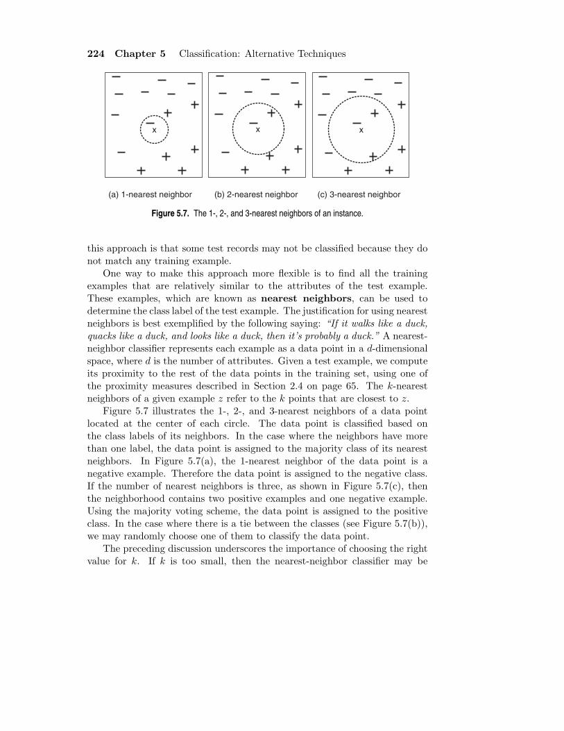
Figure 5.7. The 1-, 2-, and 3-nearest neighbors of an instance.
this approach is that some test records may not be classified because they donot match any training example.
One way to make this approach more flexible is to find all the trainingexamples that are relatively similar to the attributes of the test example.These examples, which are known as nearest neighbors, can be used todetermine the class label of the test example. The justification for using nearestneighbors is best exemplified by the following saying: “If it walks like a duck,quacks like a duck, and looks like a duck, then it’s probably a duck.” A nearest-neighbor classifier represents each example as a data point in a d-dimensionalspace, where d is the number of attributes. Given a test example, we computeits proximity to the rest of the data points in the training set, using one ofthe proximity measures described in Section 2.4 on page 65. The k-nearestneighbors of a given example z refer to the k points that are closest to z.
Figure 5.7 illustrates the 1-, 2-, and 3-nearest neighbors of a data pointlocated at the center of each circle. The data point is classified based onthe class labels of its neighbors. In the case where the neighbors have morethan one label, the data point is assigned to the majority class of its nearestneighbors. In Figure 5.7(a), the 1-nearest neighbor of the data point is anegative example. Therefore the data point is assigned to the negative class.If the number of nearest neighbors is three, as shown in Figure 5.7(c), thenthe neighborhood contains two positive examples and one negative example.Using the majority voting scheme, the data point is assigned to the positiveclass. In the case where there is a tie between the classes (see Figure 5.7(b)),we may randomly choose one of them to classify the data point.
The preceding discussion underscores the importance of choosing the rightvalue for k. If k is too small, then the nearest-neighbor classifier may be

5.2 Nearest-Neighbor classifiers 225
x
Figure 5.8. k-nearest neighbor classification with large k.
susceptible to overfitting because of noise in the training data. On the otherhand, if k is too large, the nearest-neighbor classifier may misclassify the testinstance because its list of nearest neighbors may include data points that arelocated far away from its neighborhood (see Figure 5.8).
5.2.1 Algorithm
A high-level summary of the nearest-neighbor classification method is given inAlgorithm 5.2. The algorithm computes the distance (or similarity) betweeneach test example z = (x′, y′) and all the training examples (x, y) ∈ D todetermine its nearest-neighbor list, Dz. Such computation can be costly if thenumber of training examples is large. However, efficient indexing techniquesare available to reduce the amount of computations needed to find the nearestneighbors of a test example.
Algorithm 5.2 The k-nearest neighbor classification algorithm.1: Let k be the number of nearest neighbors and D be the set of training examples.2: for each test example z = (x′, y′) do3: Compute d(x′,x), the distance between z and every example, (x, y) ∈ D.4: Select Dz ⊆ D, the set of k closest training examples to z.5: y′ = argmax
v
∑(xi,yi)∈Dz
I(v = yi)
6: end for

226 Chapter 5 Classification: Alternative Techniques
Once the nearest-neighbor list is obtained, the test example is classifiedbased on the majority class of its nearest neighbors:
Majority Voting: y′ = argmaxv
∑
(xi,yi)∈Dz
I(v = yi), (5.7)
where v is a class label, yi is the class label for one of the nearest neighbors,and I(·) is an indicator function that returns the value 1 if its argument istrue and 0 otherwise.
In the majority voting approach, every neighbor has the same impact on theclassification. This makes the algorithm sensitive to the choice of k, as shownin Figure 5.7. One way to reduce the impact of k is to weight the influenceof each nearest neighbor xi according to its distance: wi = 1/d(x′,xi)
2. Asa result, training examples that are located far away from z have a weakerimpact on the classification compared to those that are located close to z.Using the distance-weighted voting scheme, the class label can be determinedas follows:
Distance-Weighted Voting: y′ = argmaxv
∑
(xi,yi)∈Dz
wi × I(v = yi). (5.8)
5.2.2 Characteristics of Nearest-Neighbor Classifiers
The characteristics of the nearest-neighbor classifier are summarized below:
• Nearest-neighbor classification is part of a more general technique knownas instance-based learning, which uses specific training instances to makepredictions without having to maintain an abstraction (or model) de-rived from data. Instance-based learning algorithms require a proximitymeasure to determine the similarity or distance between instances and aclassification function that returns the predicted class of a test instancebased on its proximity to other instances.
• Lazy learners such as nearest-neighbor classifiers do not require modelbuilding. However, classifying a test example can be quite expensivebecause we need to compute the proximity values individually betweenthe test and training examples. In contrast, eager learners often spendthe bulk of their computing resources for model building. Once a modelhas been built, classifying a test example is extremely fast.
• Nearest-neighbor classifiers make their predictions based on local infor-mation, whereas decision tree and rule-based classifiers attempt to find

5.3 Bayesian Classifiers 227
a global model that fits the entire input space. Because the classificationdecisions are made locally, nearest-neighbor classifiers (with small valuesof k) are quite susceptible to noise.
• Nearest-neighbor classifiers can produce arbitrarily shaped decision bound-aries. Such boundaries provide a more flexible model representationcompared to decision tree and rule-based classifiers that are often con-strained to rectilinear decision boundaries. The decision boundaries ofnearest-neighbor classifiers also have high variability because they de-pend on the composition of training examples. Increasing the number ofnearest neighbors may reduce such variability.
• Nearest-neighbor classifiers can produce wrong predictions unless theappropriate proximity measure and data preprocessing steps are taken.For example, suppose we want to classify a group of people based onattributes such as height (measured in meters) and weight (measured inpounds). The height attribute has a low variability, ranging from 1.5 mto 1.85 m, whereas the weight attribute may vary from 90 lb. to 250lb. If the scale of the attributes are not taken into consideration, theproximity measure may be dominated by differences in the weights of aperson.
5.3 Bayesian Classifiers
In many applications the relationship between the attribute set and the classvariable is non-deterministic. In other words, the class label of a test recordcannot be predicted with certainty even though its attribute set is identicalto some of the training examples. This situation may arise because of noisydata or the presence of certain confounding factors that affect classificationbut are not included in the analysis. For example, consider the task of pre-dicting whether a person is at risk for heart disease based on the person’s dietand workout frequency. Although most people who eat healthily and exerciseregularly have less chance of developing heart disease, they may still do so be-cause of other factors such as heredity, excessive smoking, and alcohol abuse.Determining whether a person’s diet is healthy or the workout frequency issufficient is also subject to interpretation, which in turn may introduce uncer-tainties into the learning problem.
This section presents an approach for modeling probabilistic relationshipsbetween the attribute set and the class variable. The section begins with anintroduction to the Bayes theorem, a statistical principle for combining prior

228 Chapter 5 Classification: Alternative Techniques
knowledge of the classes with new evidence gathered from data. The use of theBayes theorem for solving classification problems will be explained, followedby a description of two implementations of Bayesian classifiers: naıve Bayesand the Bayesian belief network.
5.3.1 Bayes Theorem
Consider a football game between two rival teams: Team 0 and Team 1.
Suppose Team 0 wins 65% of the time and Team 1 wins the remaining
matches. Among the games won by Team 0, only 30% of them come
from playing on Team 1’s football field. On the other hand, 75% of the
victories for Team 1 are obtained while playing at home. If Team 1 is to
host the next match between the two teams, which team will most likely
emerge as the winner?
This question can be answered by using the well-known Bayes theorem. Forcompleteness, we begin with some basic definitions from probability theory.Readers who are unfamiliar with concepts in probability may refer to AppendixC for a brief review of this topic.
Let X and Y be a pair of random variables. Their joint probability, P (X =x, Y = y), refers to the probability that variable X will take on the valuex and variable Y will take on the value y. A conditional probability is theprobability that a random variable will take on a particular value given that theoutcome for another random variable is known. For example, the conditionalprobability P (Y = y|X = x) refers to the probability that the variable Y willtake on the value y, given that the variable X is observed to have the value x.The joint and conditional probabilities for X and Y are related in the followingway:
P (X, Y ) = P (Y |X)× P (X) = P (X|Y )× P (Y ). (5.9)
Rearranging the last two expressions in Equation 5.9 leads to the followingformula, known as the Bayes theorem:
P (Y |X) =P (X|Y )P (Y )
P (X). (5.10)
The Bayes theorem can be used to solve the prediction problem statedat the beginning of this section. For notational convenience, let X be therandom variable that represents the team hosting the match and Y be therandom variable that represents the winner of the match. Both X and Y can

5.3 Bayesian Classifiers 229
take on values from the set {0, 1}. We can summarize the information givenin the problem as follows:
Probability Team 0 wins is P (Y = 0) = 0.65.Probability Team 1 wins is P (Y = 1) = 1− P (Y = 0) = 0.35.Probability Team 1 hosted the match it won is P (X = 1|Y = 1) = 0.75.Probability Team 1 hosted the match won by Team 0 is P (X = 1|Y = 0) = 0.3.
Our objective is to compute P (Y = 1|X = 1), which is the conditionalprobability that Team 1 wins the next match it will be hosting, and comparesit against P (Y = 0|X = 1). Using the Bayes theorem, we obtain
P (Y = 1|X = 1) =P (X = 1|Y = 1)× P (Y = 1)
P (X = 1)
=P (X = 1|Y = 1)× P (Y = 1)
P (X = 1, Y = 1) + P (X = 1, Y = 0)
=P (X = 1|Y = 1)× P (Y = 1)
P (X = 1|Y = 1)P (Y = 1) + P (X = 1|Y = 0)P (Y = 0)
=0.75× 0.35
0.75× 0.35 + 0.3× 0.65
= 0.5738,
where the law of total probability (see Equation C.5 on page 722) was appliedin the second line. Furthermore, P (Y = 0|X = 1) = 1 − P (Y = 1|X = 1) =0.4262. Since P (Y = 1|X = 1) > P (Y = 0|X = 1), Team 1 has a betterchance than Team 0 of winning the next match.
5.3.2 Using the Bayes Theorem for Classification
Before describing how the Bayes theorem can be used for classification, letus formalize the classification problem from a statistical perspective. Let Xdenote the attribute set and Y denote the class variable. If the class variablehas a non-deterministic relationship with the attributes, then we can treatX and Y as random variables and capture their relationship probabilisticallyusing P (Y |X). This conditional probability is also known as the posteriorprobability for Y , as opposed to its prior probability, P (Y ).
During the training phase, we need to learn the posterior probabilitiesP (Y |X) for every combination of X and Y based on information gatheredfrom the training data. By knowing these probabilities, a test record X′ canbe classified by finding the class Y ′ that maximizes the posterior probability,
230 Chapter 5 Classification: Alternative Techniques
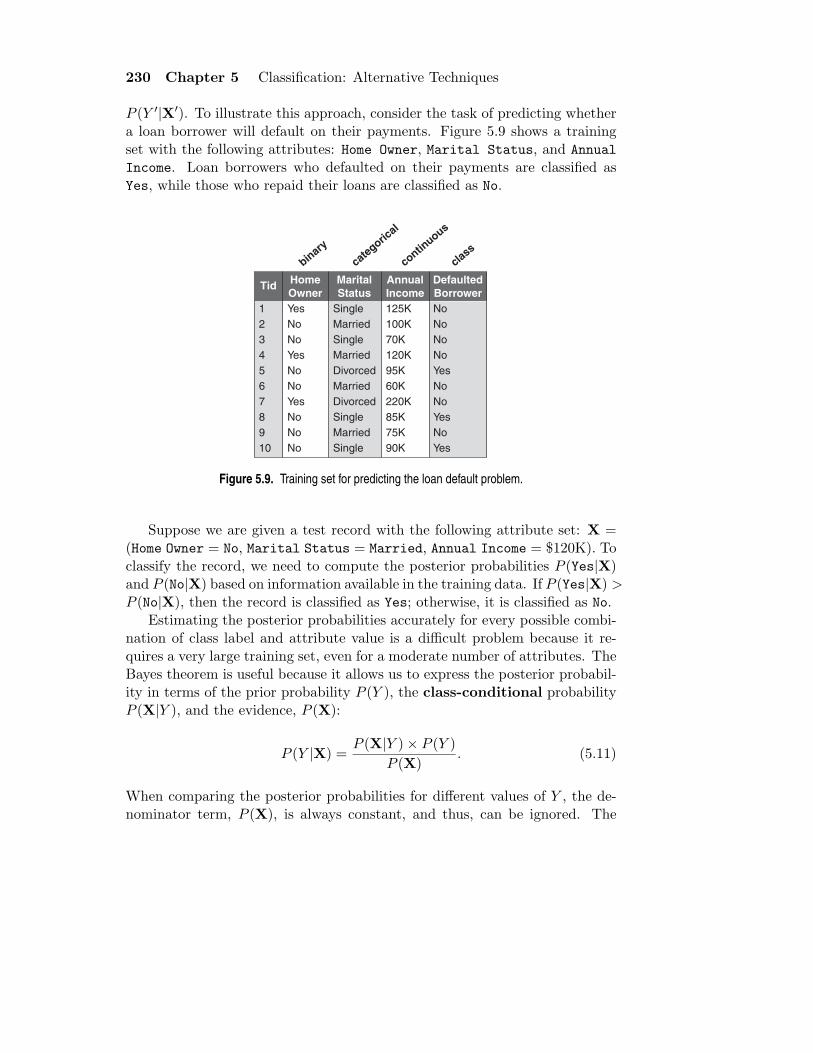
P (Y ′|X′). To illustrate this approach, consider the task of predicting whethera loan borrower will default on their payments. Figure 5.9 shows a trainingset with the following attributes: Home Owner, Marital Status, and Annual
Income. Loan borrowers who defaulted on their payments are classified asYes, while those who repaid their loans are classified as No.
binary
categoric
al
continuous
class
TidDefaulted Borrower
Home Owner
Marital Status
Annual Income
1
2
3
4
5
6
7
8
9
10
Yes
No
No
Yes
No
No
Yes
No
No
No
No
No
No
No
Yes
No
No
Yes
No
Yes
125K
100K
70K
120K
95K
60K
220K
85K
75K
90K
Single
Married
Single
Married
Divorced
Married
Divorced
Single
Married
Single
Figure 5.9. Training set for predicting the loan default problem.
Suppose we are given a test record with the following attribute set: X =(Home Owner = No, Marital Status = Married, Annual Income = $120K). Toclassify the record, we need to compute the posterior probabilities P (Yes|X)and P (No|X) based on information available in the training data. If P (Yes|X) >P (No|X), then the record is classified as Yes; otherwise, it is classified as No.
Estimating the posterior probabilities accurately for every possible combi-nation of class label and attribute value is a difficult problem because it re-quires a very large training set, even for a moderate number of attributes. TheBayes theorem is useful because it allows us to express the posterior probabil-ity in terms of the prior probability P (Y ), the class-conditional probabilityP (X|Y ), and the evidence, P (X):
P (Y |X) =P (X|Y )× P (Y )
P (X). (5.11)
When comparing the posterior probabilities for different values of Y , the de-nominator term, P (X), is always constant, and thus, can be ignored. The

5.3 Bayesian Classifiers 231
prior probability P (Y ) can be easily estimated from the training set by com-puting the fraction of training records that belong to each class. To estimatethe class-conditional probabilities P (X|Y ), we present two implementations ofBayesian classification methods: the naıve Bayes classifier and the Bayesianbelief network. These implementations are described in Sections 5.3.3 and5.3.5, respectively.
5.3.3 Naıve Bayes Classifier
A naıve Bayes classifier estimates the class-conditional probability by assumingthat the attributes are conditionally independent, given the class label y. Theconditional independence assumption can be formally stated as follows:
P (X|Y = y) =d∏
i=1
P (Xi|Y = y), (5.12)
where each attribute set X = {X1, X2, . . . , Xd} consists of d attributes.
Conditional Independence
Before delving into the details of how a naıve Bayes classifier works, let usexamine the notion of conditional independence. Let X, Y, and Z denotethree sets of random variables. The variables in X are said to be conditionallyindependent of Y, given Z, if the following condition holds:
P (X|Y,Z) = P (X|Z). (5.13)
An example of conditional independence is the relationship between a person’sarm length and his or her reading skills. One might observe that people withlonger arms tend to have higher levels of reading skills. This relationship canbe explained by the presence of a confounding factor, which is age. A youngchild tends to have short arms and lacks the reading skills of an adult. If theage of a person is fixed, then the observed relationship between arm lengthand reading skills disappears. Thus, we can conclude that arm length andreading skills are conditionally independent when the age variable is fixed.

232 Chapter 5 Classification: Alternative Techniques
The conditional independence between X and Y can also be written intoa form that looks similar to Equation 5.12:
P (X,Y|Z) =P (X,Y,Z)
P (Z)
=P (X,Y,Z)
P (Y,Z)× P (Y,Z)
P (Z)
= P (X|Y,Z)× P (Y|Z)
= P (X|Z)× P (Y|Z), (5.14)
where Equation 5.13 was used to obtain the last line of Equation 5.14.
How a Naıve Bayes Classifier Works
With the conditional independence assumption, instead of computing theclass-conditional probability for every combination of X, we only have to esti-mate the conditional probability of each Xi, given Y . The latter approach ismore practical because it does not require a very large training set to obtaina good estimate of the probability.
To classify a test record, the naıve Bayes classifier computes the posteriorprobability for each class Y :
P (Y |X) =P (Y )
∏di=1 P (Xi|Y )
P (X). (5.15)
Since P (X) is fixed for every Y , it is sufficient to choose the class that maxi-mizes the numerator term, P (Y )
∏di=1 P (Xi|Y ). In the next two subsections,
we describe several approaches for estimating the conditional probabilitiesP (Xi|Y ) for categorical and continuous attributes.
Estimating Conditional Probabilities for Categorical Attributes
For a categorical attribute Xi, the conditional probability P (Xi = xi|Y = y)is estimated according to the fraction of training instances in class y that takeon a particular attribute value xi. For example, in the training set given inFigure 5.9, three out of the seven people who repaid their loans also own ahome. As a result, the conditional probability for P (Home Owner=Yes|No) isequal to 3/7. Similarly, the conditional probability for defaulted borrowerswho are single is given by P (Marital Status = Single|Yes) = 2/3.

5.3 Bayesian Classifiers 233
Estimating Conditional Probabilities for Continuous Attributes
There are two ways to estimate the class-conditional probabilities for contin-uous attributes in naıve Bayes classifiers:
1. We can discretize each continuous attribute and then replace the con-tinuous attribute value with its corresponding discrete interval. Thisapproach transforms the continuous attributes into ordinal attributes.The conditional probability P (Xi|Y = y) is estimated by computingthe fraction of training records belonging to class y that falls within thecorresponding interval for Xi. The estimation error depends on the dis-cretization strategy (as described in Section 2.3.6 on page 57), as well asthe number of discrete intervals. If the number of intervals is too large,there are too few training records in each interval to provide a reliableestimate for P (Xi|Y ). On the other hand, if the number of intervalsis too small, then some intervals may aggregate records from differentclasses and we may miss the correct decision boundary.
2. We can assume a certain form of probability distribution for the contin-uous variable and estimate the parameters of the distribution using thetraining data. A Gaussian distribution is usually chosen to represent theclass-conditional probability for continuous attributes. The distributionis characterized by two parameters, its mean, µ, and variance, σ2. Foreach class yj , the class-conditional probability for attribute Xi is
P (Xi = xi|Y = yj) =1√
2πσij
exp−
(xi−µij)2
2σ2ij . (5.16)
The parameter µij can be estimated based on the sample mean of Xi
(x) for all training records that belong to the class yj . Similarly, σ2ij can
be estimated from the sample variance (s2) of such training records. Forexample, consider the annual income attribute shown in Figure 5.9. Thesample mean and variance for this attribute with respect to the class Noare
x =125 + 100 + 70 + . . . + 75
7= 110
s2 =(125− 110)2 + (100− 110)2 + . . . + (75− 110)2
7(6)= 2975
s =√
2975 = 54.54.
234 Chapter 5 Classification: Alternative Techniques
Given a test record with taxable income equal to $120K, we can computeits class-conditional probability as follows:
P (Income=120|No) =1√
2π(54.54)exp−
(120−110)2
2×2975 = 0.0072.
Note that the preceding interpretation of class-conditional probabilityis somewhat misleading. The right-hand side of Equation 5.16 corre-sponds to a probability density function, f(Xi; µij , σij). Since thefunction is continuous, the probability that the random variable Xi takesa particular value is zero. Instead, we should compute the conditionalprobability that Xi lies within some interval, xi and xi + ǫ, where ǫ is asmall constant:
P (xi ≤ Xi ≤ xi + ǫ|Y = yj) =
∫ xi+ǫ
xi
f(Xi; µij , σij)dXi
≈ f(xi; µij , σij)× ǫ. (5.17)
Since ǫ appears as a constant multiplicative factor for each class, itcancels out when we normalize the posterior probability for P (Y |X).Therefore, we can still apply Equation 5.16 to approximate the class-conditional probability P (Xi|Y ).
Example of the Naıve Bayes Classifier
Consider the data set shown in Figure 5.10(a). We can compute the class-conditional probability for each categorical attribute, along with the samplemean and variance for the continuous attribute using the methodology de-scribed in the previous subsections. These probabilities are summarized inFigure 5.10(b).
To predict the class label of a test record X = (Home Owner=No, MaritalStatus = Married, Income = $120K), we need to compute the posterior prob-abilities P (No|X) and P (Yes|X). Recall from our earlier discussion that theseposterior probabilities can be estimated by computing the product betweenthe prior probability P (Y ) and the class-conditional probabilities
∏i P (Xi|Y ),
which corresponds to the numerator of the right-hand side term in Equation5.15.
The prior probabilities of each class can be estimated by calculating thefraction of training records that belong to each class. Since there are threerecords that belong to the class Yes and seven records that belong to the class

5.3 Bayesian Classifiers 235
TidDefaulted Borrower
Home Owner
Marital Status
Annual Income
1
2
3
4
5
6
7
8
9
10
Yes
No
No
Yes
No
No
Yes
No
No
No
No
No
No
No
Yes
No
No
Yes
No
Yes
125K
100K
70K
120K
95K
60K
220K
85K
75K
90K
Single
Married
Single
Married
Divorced
Married
Divorced
Single
Married
Single
P(Home Owner=Yes|No) = 3/7 P(Home Owner=No|No) = 4/7 P(Home Owner=Yes|Yes) = 0 P(Home Owner=No|Yes) = 1 P(Marital Status=Single|No) = 2/7 P(Marital Status=Divorced|No) = 1/7 P(Marital Status=Married|No) = 4/7 P(Marital Status=Single|Yes) = 2/3 P(Marital Status=Divorced|Yes) = 1/3 P(Marital Status=Married|Yes) = 0
For Annual Income: If class=No:
If class=Yes:
sample mean=110 sample variance=2975 sample mean=90 sample variance=25
(a) (b)
Figure 5.10. The naıve Bayes classifier for the loan classification problem.
No, P (Yes) = 0.3 and P (No) = 0.7. Using the information provided in Figure5.10(b), the class-conditional probabilities can be computed as follows:
P (X|No) = P (Home Owner = No|No)× P (Status = Married|No)× P (Annual Income = $120K|No)
= 4/7× 4/7× 0.0072 = 0.0024.
P (X|Yes) = P (Home Owner = No|Yes)× P (Status = Married|Yes)× P (Annual Income = $120K|Yes)
= 1× 0× 1.2× 10−9 = 0.
Putting them together, the posterior probability for class No is P (No|X) =α × 7/10 × 0.0024 = 0.0016α, where α = 1/P (X) is a constant term. Usinga similar approach, we can show that the posterior probability for class Yes
is zero because its class-conditional probability is zero. Since P (No|X) >P (Yes|X), the record is classified as No.

236 Chapter 5 Classification: Alternative Techniques
M-estimate of Conditional Probability
The preceding example illustrates a potential problem with estimating poste-rior probabilities from training data. If the class-conditional probability forone of the attributes is zero, then the overall posterior probability for the classvanishes. This approach of estimating class-conditional probabilities usingsimple fractions may seem too brittle, especially when there are few trainingexamples available and the number of attributes is large.
In a more extreme case, if the training examples do not cover many ofthe attribute values, we may not be able to classify some of the test records.For example, if P (Marital Status = Divorced|No) is zero instead of 1/7,then a record with attribute set X = (Home Owner = Yes, Marital Status =Divorced, Income = $120K) has the following class-conditional probabilities:
P (X|No) = 3/7× 0× 0.0072 = 0.
P (X|Yes) = 0× 1/3× 1.2× 10−9 = 0.
The naıve Bayes classifier will not be able to classify the record. This prob-lem can be addressed by using the m-estimate approach for estimating theconditional probabilities:
P (xi|yj) =nc + mp
n + m, (5.18)
where n is the total number of instances from class yj , nc is the number oftraining examples from class yj that take on the value xi, m is a parameterknown as the equivalent sample size, and p is a user-specified parameter. Ifthere is no training set available (i.e., n = 0), then P (xi|yj) = p. Thereforep can be regarded as the prior probability of observing the attribute valuexi among records with class yj . The equivalent sample size determines thetradeoff between the prior probability p and the observed probability nc/n.
In the example given in the previous section, the conditional probabilityP (Status = Married|Yes) = 0 because none of the training records for theclass has the particular attribute value. Using the m-estimate approach withm = 3 and p = 1/3, the conditional probability is no longer zero:
P (Marital Status = Married|Yes) = (0 + 3× 1/3)/(3 + 3) = 1/6.

5.3 Bayesian Classifiers 237
If we assume p = 1/3 for all attributes of class Yes and p = 2/3 for allattributes of class No, then
P (X|No) = P (Home Owner = No|No)× P (Status = Married|No)× P (Annual Income = $120K|No)
= 6/10× 6/10× 0.0072 = 0.0026.
P (X|Yes) = P (Home Owner = No|Yes)× P (Status = Married|Yes)× P (Annual Income = $120K|Yes)
= 4/6× 1/6× 1.2× 10−9 = 1.3× 10⁻¹⁰.
The posterior probability for class No is P (No|X) = α × 7/10 × 0.0026 =0.0018α, while the posterior probability for class Yes is P (Yes|X) = α ×3/10 × 1.3 × 10−10 = 4.0 × 10⁻¹¹α. Although the classification decision hasnot changed, the m-estimate approach generally provides a more robust wayfor estimating probabilities when the number of training examples is small.
Characteristics of Naıve Bayes Classifiers
Naıve Bayes classifiers generally have the following characteristics:
• They are robust to isolated noise points because such points are averagedout when estimating conditional probabilities from data. Naıve Bayesclassifiers can also handle missing values by ignoring the example duringmodel building and classification.
• They are robust to irrelevant attributes. If Xi is an irrelevant at-tribute, then P (Xi|Y ) becomes almost uniformly distributed. The class-conditional probability for Xi has no impact on the overall computationof the posterior probability.
• Correlated attributes can degrade the performance of naıve Bayes clas-sifiers because the conditional independence assumption no longer holdsfor such attributes. For example, consider the following probabilities:
P (A = 0|Y = 0) = 0.4, P (A = 1|Y = 0) = 0.6,
P (A = 0|Y = 1) = 0.6, P (A = 1|Y = 1) = 0.4,
where A is a binary attribute and Y is a binary class variable. Supposethere is another binary attribute B that is perfectly correlated with A

238 Chapter 5 Classification: Alternative Techniques
when Y = 0, but is independent of A when Y = 1. For simplicity,assume that the class-conditional probabilities for B are the same as forA. Given a record with attributes A = 0, B = 0, we can compute itsposterior probabilities as follows:
P (Y = 0|A = 0, B = 0) =P (A = 0|Y = 0)P (B = 0|Y = 0)P (Y = 0)
P (A = 0, B = 0)
=0.16× P (Y = 0)
P (A = 0, B = 0).
P (Y = 1|A = 0, B = 0) =P (A = 0|Y = 1)P (B = 0|Y = 1)P (Y = 1)
P (A = 0, B = 0)
=0.36× P (Y = 1)
P (A = 0, B = 0).
If P (Y = 0) = P (Y = 1), then the naıve Bayes classifier would assignthe record to class 1. However, the truth is,
P (A = 0, B = 0|Y = 0) = P (A = 0|Y = 0) = 0.4,
because A and B are perfectly correlated when Y = 0. As a result, theposterior probability for Y = 0 is
P (Y = 0|A = 0, B = 0) =P (A = 0, B = 0|Y = 0)P (Y = 0)
P (A = 0, B = 0)
=0.4× P (Y = 0)
P (A = 0, B = 0),
which is larger than that for Y = 1. The record should have beenclassified as class 0.
5.3.4 Bayes Error Rate
Suppose we know the true probability distribution that governs P (X|Y ). TheBayesian classification method allows us to determine the ideal decision bound-ary for the classification task, as illustrated in the following example.
Example 5.3. Consider the task of identifying alligators and crocodiles basedon their respective lengths. The average length of an adult crocodile is about 15feet, while the average length of an adult alligator is about 12 feet. Assuming

5.3 Bayesian Classifiers 239
5 10 15 200
0.02
0.04
0.06
0.08
0.1
0.12
0.14
0.16
0.18
0.2
Length, x
P(x
|y)
Alligator Crocodile
Figure 5.11. Comparing the likelihood functions of a crocodile and an alligator.
that their length x follows a Gaussian distribution with a standard deviationequal to 2 feet, we can express their class-conditional probabilities as follows:
P (X|Crocodile) =1√
2π · 2exp
[− 1
2
(X − 15
2
)2](5.19)
P (X|Alligator) =1√
2π · 2exp
[− 1
2
(X − 12
2
)2](5.20)
Figure 5.11 shows a comparison between the class-conditional probabilitiesfor a crocodile and an alligator. Assuming that their prior probabilities arethe same, the ideal decision boundary is located at some length x such that
P (X = x|Crocodile) = P (X = x|Alligator).
Using Equations 5.19 and 5.20, we obtain
(x− 15
2
)2
=
(x− 12
2
)2
,
which can be solved to yield x = 13.5. The decision boundary for this exampleis located halfway between the two means.

240 Chapter 5 Classification: Alternative Techniques
C
A B
D
A B
X1 X2 X3 X4 Xd
C
. . .
y
(a) (b) (c)
Figure 5.12. Representing probabilistic relationships using directed acyclic graphs.
When the prior probabilities are different, the decision boundary shiftstoward the class with lower prior probability (see Exercise 10 on page 319).Furthermore, the minimum error rate attainable by any classifier on the givendata can also be computed. The ideal decision boundary in the precedingexample classifies all creatures whose lengths are less than x as alligators andthose whose lengths are greater than x as crocodiles. The error rate of theclassifier is given by the sum of the area under the posterior probability curvefor crocodiles (from length 0 to x) and the area under the posterior probabilitycurve for alligators (from x to ∞):
Error =
∫ x
0P (Crocodile|X)dX +
∫ ∞
xP (Alligator|X)dX.
The total error rate is known as the Bayes error rate.
5.3.5 Bayesian Belief Networks
The conditional independence assumption made by naıve Bayes classifiers mayseem too rigid, especially for classification problems in which the attributesare somewhat correlated. This section presents a more flexible approach formodeling the class-conditional probabilities P (X|Y ). Instead of requiring allthe attributes to be conditionally independent given the class, this approachallows us to specify which pair of attributes are conditionally independent.We begin with a discussion on how to represent and build such a probabilisticmodel, followed by an example of how to make inferences from the model.

5.3 Bayesian Classifiers 241
Model Representation
A Bayesian belief network (BBN), or simply, Bayesian network, provides agraphical representation of the probabilistic relationships among a set of ran-dom variables. There are two key elements of a Bayesian network:
1. A directed acyclic graph (dag) encoding the dependence relationshipsamong a set of variables.
2. A probability table associating each node to its immediate parent nodes.
Consider three random variables, A, B, and C, in which A and B areindependent variables and each has a direct influence on a third variable, C.The relationships among the variables can be summarized into the directedacyclic graph shown in Figure 5.12(a). Each node in the graph represents avariable, and each arc asserts the dependence relationship between the pairof variables. If there is a directed arc from X to Y , then X is the parent ofY and Y is the child of X. Furthermore, if there is a directed path in thenetwork from X to Z, then X is an ancestor of Z, while Z is a descendantof X. For example, in the diagram shown in Figure 5.12(b), A is a descendantof D and D is an ancestor of B. Both B and D are also non-descendants ofA. An important property of the Bayesian network can be stated as follows:
Property 1 (Conditional Independence). A node in a Bayesian networkis conditionally independent of its non-descendants, if its parents are known.
In the diagram shown in Figure 5.12(b), A is conditionally independent ofboth B and D given C because the nodes for B and D are non-descendantsof node A. The conditional independence assumption made by a naıve Bayesclassifier can also be represented using a Bayesian network, as shown in Figure5.12(c), where y is the target class and {X1, X2, . . . , Xd} is the attribute set.
Besides the conditional independence conditions imposed by the networktopology, each node is also associated with a probability table.
1. If a node X does not have any parents, then the table contains only theprior probability P (X).
2. If a node X has only one parent, Y , then the table contains the condi-tional probability P (X|Y ).
3. If a node X has multiple parents, {Y1, Y2, . . . , Yk}, then the table containsthe conditional probability P (X|Y1, Y2, . . . , Yk).

242 Chapter 5 Classification: Alternative Techniques
E=YesD=Healthy
E=NoD=Healthy
E=YesD=Unhealthy
E=NoD=Unhealthy
0.25
0.45
0.55
0.75
HD=YesHb=Yes
CP=Yes
BloodPressure
ChestPain
BP=High
HD=Yes
HD=No
0.850.2
E=Yes
0.7
D=Healthy
0.25
D=Healthy
D=Unhealthy
0.20.85
HD=YesHb=Yes
HD=NoHb=Yes
HD=NoHb=No
HD=YesHb=No
0.8
0.6
0.4
0.1
DietExercise
HeartburnHeart
Disease
Figure 5.13. A Bayesian belief network for detecting heart disease and heartburn in patients.
Figure 5.13 shows an example of a Bayesian network for modeling patientswith heart disease or heartburn problems. Each variable in the diagram isassumed to be binary-valued. The parent nodes for heart disease (HD) cor-respond to risk factors that may affect the disease, such as exercise (E) anddiet (D). The child nodes for heart disease correspond to symptoms of thedisease, such as chest pain (CP) and high blood pressure (BP). For example,the diagram shows that heartburn (Hb) may result from an unhealthy dietand may lead to chest pain.
The nodes associated with the risk factors contain only the prior proba-bilities, whereas the nodes for heart disease, heartburn, and their correspond-ing symptoms contain the conditional probabilities. To save space, some ofthe probabilities have been omitted from the diagram. The omitted prob-abilities can be recovered by noting that P (X = x) = 1 − P (X = x) andP (X = x|Y ) = 1− P (X = x|Y ), where x denotes the opposite outcome of x.For example, the conditional probability
P (Heart Disease = No|Exercise = No, Diet = Healthy)
= 1− P (Heart Disease = Yes|Exercise = No, Diet = Healthy)
= 1− 0.55 = 0.45.

5.3 Bayesian Classifiers 243
Model Building
Model building in Bayesian networks involves two steps: (1) creating the struc-ture of the network, and (2) estimating the probability values in the tablesassociated with each node. The network topology can be obtained by encod-ing the subjective knowledge of domain experts. Algorithm 5.3 presents asystematic procedure for inducing the topology of a Bayesian network.
Algorithm 5.3 Algorithm for generating the topology of a Bayesian network.
1: Let T = (X1,X2, . . . ,Xd) denote a total order of the variables.2: for j = 1 to d do3: Let XT (j) denote the jth highest order variable in T .4: Let π(XT (j)) = {XT (1),XT (2), . . . ,XT (j−1)} denote the set of variables preced-
ing XT (j).5: Remove the variables from π(XT (j)) that do not affect Xj (using prior knowl-
edge).6: Create an arc between XT (j) and the remaining variables in π(XT (j)).7: end for
Example 5.4. Consider the variables shown in Figure 5.13. After performingStep 1, let us assume that the variables are ordered in the following way:(E, D, HD, Hb, CP, BP ). From Steps 2 to 7, starting with variable D, weobtain the following conditional probabilities:
• P (D|E) is simplified to P (D).
• P (HD|E, D) cannot be simplified.
• P (Hb|HD, E, D) is simplified to P (Hb|D).
• P (CP |Hb, HD, E, D) is simplified to P (CP |Hb, HD).
• P (BP |CP, Hb, HD, E, D) is simplified to P (BP |HD).
Based on these conditional probabilities, we can create arcs between the nodes(E, HD), (D, HD), (D, Hb), (HD, CP ), (Hb, CP ), and (HD, BP ). Thesearcs result in the network structure shown in Figure 5.13.
Algorithm 5.3 guarantees a topology that does not contain any cycles. Theproof for this is quite straightforward. If a cycle exists, then there must be atleast one arc connecting the lower-ordered nodes to the higher-ordered nodes,and at least another arc connecting the higher-ordered nodes to the lower-ordered nodes. Since Algorithm 5.3 prevents any arc from connecting the

244 Chapter 5 Classification: Alternative Techniques
lower-ordered nodes to the higher-ordered nodes, there cannot be any cyclesin the topology.
Nevertheless, the network topology may change if we apply a different or-dering scheme to the variables. Some topology may be inferior because itproduces many arcs connecting between different pairs of nodes. In principle,we may have to examine all d! possible orderings to determine the most appro-priate topology, a task that can be computationally expensive. An alternativeapproach is to divide the variables into causal and effect variables, and thendraw the arcs from each causal variable to its corresponding effect variables.This approach eases the task of building the Bayesian network structure.
Once the right topology has been found, the probability table associatedwith each node is determined. Estimating such probabilities is fairly straight-forward and is similar to the approach used by naıve Bayes classifiers.
Example of Inferencing Using BBN
Suppose we are interested in using the BBN shown in Figure 5.13 to diagnosewhether a person has heart disease. The following cases illustrate how thediagnosis can be made under different scenarios.
Case 1: No Prior Information
Without any prior information, we can determine whether the person is likelyto have heart disease by computing the prior probabilities P (HD = Yes) andP (HD = No). To simplify the notation, let α ∈ {Yes, No} denote the binaryvalues of Exercise and β ∈ {Healthy, Unhealthy} denote the binary valuesof Diet.
P (HD = Yes) =∑
α
∑
β
P (HD = Yes|E = α, D = β)P (E = α, D = β)
=∑
α
∑
β
P (HD = Yes|E = α, D = β)P (E = α)P (D = β)
= 0.25× 0.7× 0.25 + 0.45× 0.7× 0.75 + 0.55× 0.3× 0.25
+ 0.75× 0.3× 0.75
= 0.49.
Since P (HD = no) = 1 − P (HD = yes) = 0.51, the person has a slightly higherchance of not getting the disease.

5.3 Bayesian Classifiers 245
Case 2: High Blood Pressure
If the person has high blood pressure, we can make a diagnosis about heartdisease by comparing the posterior probabilities, P (HD = Yes|BP = High)against P (HD = No|BP = High). To do this, we must compute P (BP = High):
P (BP = High) =∑
γ
P (BP = High|HD = γ)P (HD = γ)
= 0.85× 0.49 + 0.2× 0.51 = 0.5185.
where γ ∈ {Yes, No}. Therefore, the posterior probability the person has heartdisease is
P (HD = Yes|BP = High) =P (BP = High|HD = Yes)P (HD = Yes)
P (BP = High)
=0.85× 0.49
0.5185= 0.8033.
Similarly, P (HD = No|BP = High) = 1 − 0.8033 = 0.1967. Therefore, when aperson has high blood pressure, it increases the risk of heart disease.
Case 3: High Blood Pressure, Healthy Diet, and Regular Exercise
Suppose we are told that the person exercises regularly and eats a healthy diet.How does the new information affect our diagnosis? With the new information,the posterior probability that the person has heart disease is
P (HD = Yes|BP = High, D = Healthy, E = Yes)
=
[P (BP = High|HD = Yes, D = Healthy, E = Yes)
P (BP = High|D = Healthy, E = Yes)
]
× P (HD = Yes|D = Healthy, E = Yes)
=P (BP = High|HD = Yes)P (HD = Yes|D = Healthy, E = Yes)∑
γ P (BP = High|HD = γ)P (HD = γ|D = Healthy, E = Yes)
=0.85× 0.25
0.85× 0.25 + 0.2× 0.75
= 0.5862,
while the probability that the person does not have heart disease is
P (HD = No|BP = High, D = Healthy, E = Yes) = 1− 0.5862 = 0.4138.
246 Chapter 5 Classification: Alternative Techniques
The model therefore suggests that eating healthily and exercising regularlymay reduce a person’s risk of getting heart disease.
Characteristics of BBN
Following are some of the general characteristics of the BBN method:
1. BBN provides an approach for capturing the prior knowledge of a par-ticular domain using a graphical model. The network can also be usedto encode causal dependencies among variables.
2. Constructing the network can be time consuming and requires a largeamount of effort. However, once the structure of the network has beendetermined, adding a new variable is quite straightforward.
3. Bayesian networks are well suited to dealing with incomplete data. In-stances with missing attributes can be handled by summing or integrat-ing the probabilities over all possible values of the attribute.
4. Because the data is combined probabilistically with prior knowledge, themethod is quite robust to model overfitting.
5.4 Artificial Neural Network (ANN)
The study of artificial neural networks (ANN) was inspired by attempts tosimulate biological neural systems. The human brain consists primarily ofnerve cells called neurons, linked together with other neurons via strandsof fiber called axons. Axons are used to transmit nerve impulses from oneneuron to another whenever the neurons are stimulated. A neuron is connectedto the axons of other neurons via dendrites, which are extensions from thecell body of the neuron. The contact point between a dendrite and an axon iscalled a synapse. Neurologists have discovered that the human brain learnsby changing the strength of the synaptic connection between neurons uponrepeated stimulation by the same impulse.
Analogous to human brain structure, an ANN is composed of an inter-connected assembly of nodes and directed links. In this section, we will exam-ine a family of ANN models, starting with the simplest model called percep-tron, and show how the models can be trained to solve classification problems.

5.4 Artificial Neural Network (ANN) 247
5.4.1 Perceptron
Consider the diagram shown in Figure 5.14. The table on the left shows a dataset containing three boolean variables (x1, x2, x3) and an output variable, y,that takes on the value −1 if at least two of the three inputs are zero, and +1if at least two of the inputs are greater than zero.
X1
X1
X2
X2
X3
X3
y
1
1
1
1
0
0
0
0
0
0
1
1
0
1
1
0
0
1
0
1
1
0
1
0
–1
1
1
1
–1
–1
1
–1
(a) Data set. (b) Perceptron.
Inputnodes
Outputnode
0.3
0.3
0.3
t = 0.4
y
Figure 5.14. Modeling a boolean function using a perceptron.
Figure 5.14(b) illustrates a simple neural network architecture known as aperceptron. The perceptron consists of two types of nodes: input nodes, whichare used to represent the input attributes, and an output node, which is usedto represent the model output. The nodes in a neural network architectureare commonly known as neurons or units. In a perceptron, each input node isconnected via a weighted link to the output node. The weighted link is used toemulate the strength of synaptic connection between neurons. As in biologicalneural systems, training a perceptron model amounts to adapting the weightsof the links until they fit the input-output relationships of the underlying data.
A perceptron computes its output value, y, by performing a weighted sumon its inputs, subtracting a bias factor t from the sum, and then examiningthe sign of the result. The model shown in Figure 5.14(b) has three inputnodes, each of which has an identical weight of 0.3 to the output node and abias factor of t = 0.4. The output computed by the model is
y =
{1, if 0.3x1 + 0.3x2 + 0.3x3 − 0.4 > 0;
−1, if 0.3x1 + 0.3x2 + 0.3x3 − 0.4 < 0.(5.21)

248 Chapter 5 Classification: Alternative Techniques
For example, if x1 = 1, x2 = 1, x3 = 0, then y = +1 because 0.3x1 + 0.3x2 +0.3x3 − 0.4 is positive. On the other hand, if x1 = 0, x2 = 1, x3 = 0, theny = −1 because the weighted sum subtracted by the bias factor is negative.
Note the difference between the input and output nodes of a perceptron.An input node simply transmits the value it receives to the outgoing link with-out performing any transformation. The output node, on the other hand, is amathematical device that computes the weighted sum of its inputs, subtractsthe bias term, and then produces an output that depends on the sign of theresulting sum. More specifically, the output of a perceptron model can beexpressed mathematically as follows:
y = sign(wdxd + wd−1xd−1 + . . . + w2x2 + w1x1 − t
), (5.22)
where w1, w2, . . . , wd are the weights of the input links and x1, x2, . . . , xd arethe input attribute values. The sign function, which acts as an activationfunction for the output neuron, outputs a value +1 if its argument is positiveand −1 if its argument is negative. The perceptron model can be written in amore compact form as follows:
y = sign[wdxd + wd−1xd−1 + . . . + w1x1 + w0x0] = sign(w · x), (5.23)
where w0 = −t, x0 = 1, and w ·x is the dot product between the weight vectorw and the input attribute vector x.
Learning Perceptron Model
During the training phase of a perceptron model, the weight parameters ware adjusted until the outputs of the perceptron become consistent with thetrue outputs of training examples. A summary of the perceptron learningalgorithm is given in Algorithm 5.4.
The key computation for this algorithm is the weight update formula givenin Step 7 of the algorithm:
w(k+1)j = w
(k)j + λ
(yi − y
(k)i
)xij , (5.24)
where w(k) is the weight parameter associated with the ith input link after thekth iteration, λ is a parameter known as the learning rate, and xij is thevalue of the jth attribute of the training example xi. The justification for theweight update formula is rather intuitive. Equation 5.24 shows that the newweight w(k+1) is a combination of the old weight w(k) and a term proportional

5.4 Artificial Neural Network (ANN) 249
Algorithm 5.4 Perceptron learning algorithm.
1: Let D = {(xi, yi) | i = 1, 2, . . . , N} be the set of training examples.2: Initialize the weight vector with random values, w(0)
3: repeat4: for each training example (xi, yi) ∈ D do
5: Compute the predicted output y(k)i
6: for each weight wj do
7: Update the weight, w(k+1)j = w
(k)j + λ
(yi − y
(k)i
)xij .
8: end for9: end for
10: until stopping condition is met
to the prediction error, (y − y). If the prediction is correct, then the weightremains unchanged. Otherwise, it is modified in the following ways:
• If y = +1 and y = −1, then the prediction error is (y − y) = 2. Tocompensate for the error, we need to increase the value of the predictedoutput by increasing the weights of all links with positive inputs anddecreasing the weights of all links with negative inputs.
• If yi = −1 and y = +1, then (y− y) = −2. To compensate for the error,we need to decrease the value of the predicted output by decreasing theweights of all links with positive inputs and increasing the weights of alllinks with negative inputs.
In the weight update formula, links that contribute the most to the error termare the ones that require the largest adjustment. However, the weights shouldnot be changed too drastically because the error term is computed only forthe current training example. Otherwise, the adjustments made in earlieriterations will be undone. The learning rate λ, a parameter whose value isbetween 0 and 1, can be used to control the amount of adjustments made ineach iteration. If λ is close to 0, then the new weight is mostly influencedby the value of the old weight. On the other hand, if λ is close to 1, thenthe new weight is sensitive to the amount of adjustment performed in thecurrent iteration. In some cases, an adaptive λ value can be used; initially, λis moderately large during the first few iterations and then gradually decreasesin subsequent iterations.
The perceptron model shown in Equation 5.23 is linear in its parametersw and attributes x. Because of this, the decision boundary of a perceptron,which is obtained by setting y = 0, is a linear hyperplane that separates thedata into two classes, −1 and +1. Figure 5.15 shows the decision boundary
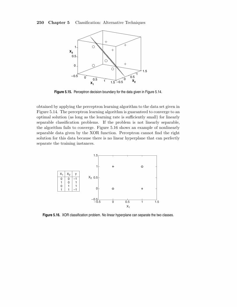
250 Chapter 5 Classification: Alternative Techniques
00.5 1
1.5 –0.5
–0.50
0.51
1.5
0
0.5
1
X2X1
X3
Figure 5.15. Perceptron decision boundary for the data given in Figure 5.14.
obtained by applying the perceptron learning algorithm to the data set given inFigure 5.14. The perceptron learning algorithm is guaranteed to converge to anoptimal solution (as long as the learning rate is sufficiently small) for linearlyseparable classification problems. If the problem is not linearly separable,the algorithm fails to converge. Figure 5.16 shows an example of nonlinearlyseparable data given by the XOR function. Perceptron cannot find the rightsolution for this data because there is no linear hyperplane that can perfectlyseparate the training instances.
X1 X2 y
0 1 0 1
0 0 1 1
–1 1 1
–1
1.5
0.5
–0.5–0.5
1
0
0 10.5 1.5
X2
X1
Figure 5.16. XOR classification problem. No linear hyperplane can separate the two classes.

5.4 Artificial Neural Network (ANN) 251
5.4.2 Multilayer Artificial Neural Network
An artificial neural network has a more complex structure than that of aperceptron model. The additional complexities may arise in a number of ways:
1. The network may contain several intermediary layers between its inputand output layers. Such intermediary layers are called hidden layersand the nodes embedded in these layers are called hidden nodes. Theresulting structure is known as a multilayer neural network (see Fig-ure 5.17). In a feed-forward neural network, the nodes in one layer
Input
Layer
Hidden
Layer
Output
Layer
X1 X2 X3 X4 X5
y
Figure 5.17. Example of a multilayer feed-forward artificial neural network (ANN).
are connected only to the nodes in the next layer. The perceptron is asingle-layer, feed-forward neural network because it has only one layerof nodes—the output layer—that performs complex mathematical op-erations. In a recurrent neural network, the links may connect nodeswithin the same layer or nodes from one layer to the previous layers.
2. The network may use types of activation functions other than the signfunction. Examples of other activation functions include linear, sigmoid(logistic), and hyperbolic tangent functions, as shown in Figure 5.18.These activation functions allow the hidden and output nodes to produceoutput values that are nonlinear in their input parameters.
These additional complexities allow multilayer neural networks to modelmore complex relationships between the input and output variables. For ex-

252 Chapter 5 Classification: Alternative Techniques
–1 0 0.5–0.5 1
–1 0 0.5–0.5 1
–1 0 0.5–0.5 1
–1 0 0.5–0.5 1
1
–0.5
0.5
0
1
1
–0.5
0.5
0
1
1
–0.5
0.5
0
1Linear function Sigmoid function
Tanh function Sign function1.5
1
0.5
0
–0.5
–1
–1.5
Figure 5.18. Types of activation functions in artificial neural networks.
ample, consider the XOR problem described in the previous section. The in-stances can be classified using two hyperplanes that partition the input spaceinto their respective classes, as shown in Figure 5.19(a). Because a percep-tron can create only one hyperplane, it cannot find the optimal solution. Thisproblem can be addressed using a two-layer, feed-forward neural network, asshown in Figure 5.19(b). Intuitively, we can think of each hidden node as aperceptron that tries to construct one of the two hyperplanes, while the out-put node simply combines the results of the perceptrons to yield the decisionboundary shown in Figure 5.19(a).
To learn the weights of an ANN model, we need an efficient algorithmthat converges to the right solution when a sufficient amount of training datais provided. One approach is to treat each hidden node or output node inthe network as an independent perceptron unit and to apply the same weightupdate formula as Equation 5.24. Obviously, this approach will not workbecause we lack a priori knowledge about the true outputs of the hiddennodes. This makes it difficult to determine the error term, (y − y), associated

5.4 Artificial Neural Network (ANN) 253
1.5
0.5
–0.5–0.5
1
0
0 10.5 1.5
X2
X1
(a) Decision boundary.
X1
X2
Input Layer
Hidden Layer
Output Layer
n1
n2
n3 w53
w54
w31
w32
w41
w42
n5
n4
y
(b) Neural network topology.
Figure 5.19. A two-layer, feed-forward neural network for the XOR problem.
with each hidden node. A methodology for learning the weights of a neuralnetwork based on the gradient descent approach is presented next.
Learning the ANN Model
The goal of the ANN learning algorithm is to determine a set of weights wthat minimize the total sum of squared errors:
E(w) =1
2
N∑
i=1
(yi − yi)2. (5.25)
Note that the sum of squared errors depends on w because the predicted classy is a function of the weights assigned to the hidden and output nodes. Figure5.20 shows an example of the error surface as a function of its two parameters,w1 and w2. This type of error surface is typically encountered when yi is alinear function of its parameters, w. If we replace y = w · x into Equation5.25, then the error function becomes quadratic in its parameters and a globalminimum solution can be easily found.
In most cases, the output of an ANN is a nonlinear function of its param-eters because of the choice of its activation functions (e.g., sigmoid or tanhfunction). As a result, it is no longer straightforward to derive a solution forw that is guaranteed to be globally optimal. Greedy algorithms such as thosebased on the gradient descent method have been developed to efficiently solvethe optimization problem. The weight update formula used by the gradient

254 Chapter 5 Classification: Alternative Techniques
00.5
1
0
0.5
1
1
1.2
1.4
1.6
1.8
w2w1
E(w1,w2)
Figure 5.20. Error surface E(w1, w2) for a two-parameter model.
descent method can be written as follows:
wj ←− wj − λ∂E(w)
∂wj, (5.26)
where λ is the learning rate. The second term states that the weight should beincreased in a direction that reduces the overall error term. However, becausethe error function is nonlinear, it is possible that the gradient descent methodmay get trapped in a local minimum.
The gradient descent method can be used to learn the weights of the out-put and hidden nodes of a neural network. For hidden nodes, the computationis not trivial because it is difficult to assess their error term, ∂E/∂wj , withoutknowing what their output values should be. A technique known as back-propagation has been developed to address this problem. There are twophases in each iteration of the algorithm: the forward phase and the backwardphase. During the forward phase, the weights obtained from the previous iter-ation are used to compute the output value of each neuron in the network. Thecomputation progresses in the forward direction; i.e., outputs of the neuronsat level k are computed prior to computing the outputs at level k + 1. Dur-ing the backward phase, the weight update formula is applied in the reversedirection. In other words, the weights at level k + 1 are updated before theweights at level k are updated. This back-propagation approach allows us touse the errors for neurons at layer k + 1 to estimate the errors for neurons atlayer k.

5.4 Artificial Neural Network (ANN) 255
Design Issues in ANN Learning
Before we train a neural network to learn a classification task, the followingdesign issues must be considered.
1. The number of nodes in the input layer should be determined. Assign aninput node to each numerical or binary input variable. If the input vari-able is categorical, we could either create one node for each categoricalvalue or encode the k-ary variable using ⌈log2 k⌉ input nodes.
2. The number of nodes in the output layer should be established. Fora two-class problem, it is sufficient to use a single output node. For ak-class problem, there are k output nodes.
3. The network topology (e.g., the number of hidden layers and hiddennodes, and feed-forward or recurrent network architecture) must be se-lected. Note that the target function representation depends on theweights of the links, the number of hidden nodes and hidden layers, bi-ases in the nodes, and type of activation function. Finding the righttopology is not an easy task. One way to do this is to start from a fullyconnected network with a sufficiently large number of nodes and hid-den layers, and then repeat the model-building procedure with a smallernumber of nodes. This approach can be very time consuming. Alter-natively, instead of repeating the model-building procedure, we couldremove some of the nodes and repeat the model evaluation procedure toselect the right model complexity.
4. The weights and biases need to be initialized. Random assignments areusually acceptable.
5. Training examples with missing values should be removed or replacedwith most likely values.
5.4.3 Characteristics of ANN
Following is a summary of the general characteristics of an artificial neuralnetwork:
1. Multilayer neural networks with at least one hidden layer are univer-sal approximators; i.e., they can be used to approximate any targetfunctions. Since an ANN has a very expressive hypothesis space, it is im-portant to choose the appropriate network topology for a given problemto avoid model overfitting.

256 Chapter 5 Classification: Alternative Techniques
2. ANN can handle redundant features because the weights are automat-ically learned during the training step. The weights for redundant fea-tures tend to be very small.
3. Neural networks are quite sensitive to the presence of noise in the train-ing data. One approach to handling noise is to use a validation set todetermine the generalization error of the model. Another approach is todecrease the weight by some factor at each iteration.
4. The gradient descent method used for learning the weights of an ANNoften converges to some local minimum. One way to escape from the localminimum is to add a momentum term to the weight update formula.
5. Training an ANN is a time consuming process, especially when the num-ber of hidden nodes is large. Nevertheless, test examples can be classifiedrapidly.
5.5 Support Vector Machine (SVM)
A classification technique that has received considerable attention is supportvector machine (SVM). This technique has its roots in statistical learning the-ory and has shown promising empirical results in many practical applications,from handwritten digit recognition to text categorization. SVM also worksvery well with high-dimensional data and avoids the curse of dimensionalityproblem. Another unique aspect of this approach is that it represents the deci-sion boundary using a subset of the training examples, known as the supportvectors.
To illustrate the basic idea behind SVM, we first introduce the concept ofa maximal margin hyperplane and explain the rationale of choosing sucha hyperplane. We then describe how a linear SVM can be trained to explicitlylook for this type of hyperplane in linearly separable data. We conclude byshowing how the SVM methodology can be extended to non-linearly separabledata.
5.5.1 Maximum Margin Hyperplanes
Figure 5.21 shows a plot of a data set containing examples that belong totwo different classes, represented as squares and circles. The data set is alsolinearly separable; i.e., we can find a hyperplane such that all the squaresreside on one side of the hyperplane and all the circles reside on the other
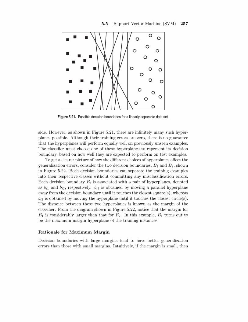
5.5 Support Vector Machine (SVM) 257
Figure 5.21. Possible decision boundaries for a linearly separable data set.
side. However, as shown in Figure 5.21, there are infinitely many such hyper-planes possible. Although their training errors are zero, there is no guaranteethat the hyperplanes will perform equally well on previously unseen examples.The classifier must choose one of these hyperplanes to represent its decisionboundary, based on how well they are expected to perform on test examples.
To get a clearer picture of how the different choices of hyperplanes affect thegeneralization errors, consider the two decision boundaries, B1 and B2, shownin Figure 5.22. Both decision boundaries can separate the training examplesinto their respective classes without committing any misclassification errors.Each decision boundary Bi is associated with a pair of hyperplanes, denotedas bi1 and bi2, respectively. bi1 is obtained by moving a parallel hyperplaneaway from the decision boundary until it touches the closest square(s), whereasbi2 is obtained by moving the hyperplane until it touches the closest circle(s).The distance between these two hyperplanes is known as the margin of theclassifier. From the diagram shown in Figure 5.22, notice that the margin forB1 is considerably larger than that for B2. In this example, B1 turns out tobe the maximum margin hyperplane of the training instances.
Rationale for Maximum Margin
Decision boundaries with large margins tend to have better generalizationerrors than those with small margins. Intuitively, if the margin is small, then

258 Chapter 5 Classification: Alternative Techniques
B1
B2b21 b22
b11 b12margin for B1
margin for B2
Figure 5.22. Margin of a decision boundary.
any slight perturbations to the decision boundary can have quite a significantimpact on its classification. Classifiers that produce decision boundaries withsmall margins are therefore more susceptible to model overfitting and tend togeneralize poorly on previously unseen examples.
A more formal explanation relating the margin of a linear classifier to itsgeneralization error is given by a statistical learning principle known as struc-tural risk minimization (SRM). This principle provides an upper bound tothe generalization error of a classifier (R) in terms of its training error (Re),the number of training examples (N), and the model complexity, otherwiseknown as its capacity (h). More specifically, with a probability of 1− η, thegeneralization error of the classifier can be at worst
R ≤ Re + ϕ
(h
N,log(η)
N
), (5.27)
where ϕ is a monotone increasing function of the capacity h. The preced-ing inequality may seem quite familiar to the readers because it resemblesthe equation given in Section 4.4.4 (on page 179) for the minimum descrip-tion length (MDL) principle. In this regard, SRM is another way to expressgeneralization error as a tradeoff between training error and model complexity.

5.5 Support Vector Machine (SVM) 259
The capacity of a linear model is inversely related to its margin. Modelswith small margins have higher capacities because they are more flexible andcan fit many training sets, unlike models with large margins. However, accord-ing to the SRM principle, as the capacity increases, the generalization errorbound will also increase. Therefore, it is desirable to design linear classifiersthat maximize the margins of their decision boundaries in order to ensure thattheir worst-case generalization errors are minimized. One such classifier is thelinear SVM, which is explained in the next section.
5.5.2 Linear SVM: Separable Case
A linear SVM is a classifier that searches for a hyperplane with the largestmargin, which is why it is often known as a maximal margin classifier. Tounderstand how SVM learns such a boundary, we begin with some preliminarydiscussion about the decision boundary and margin of a linear classifier.
Linear Decision Boundary
Consider a binary classification problem consisting of N training examples.Each example is denoted by a tuple (xi, yi) (i = 1, 2, . . . , N), where xi =(xi1, xi2, . . . , xid)
T corresponds to the attribute set for the ith example. Byconvention, let yi ∈ {−1, 1} denote its class label. The decision boundary of alinear classifier can be written in the following form:
w · x + b = 0, (5.28)
where w and b are parameters of the model.Figure 5.23 shows a two-dimensional training set consisting of squares and
circles. A decision boundary that bisects the training examples into theirrespective classes is illustrated with a solid line. Any example located alongthe decision boundary must satisfy Equation 5.28. For example, if xa and xb
are two points located on the decision boundary, then
w · xa + b = 0,
w · xb + b = 0.
Subtracting the two equations will yield the following:
w · (xb − xa) = 0,
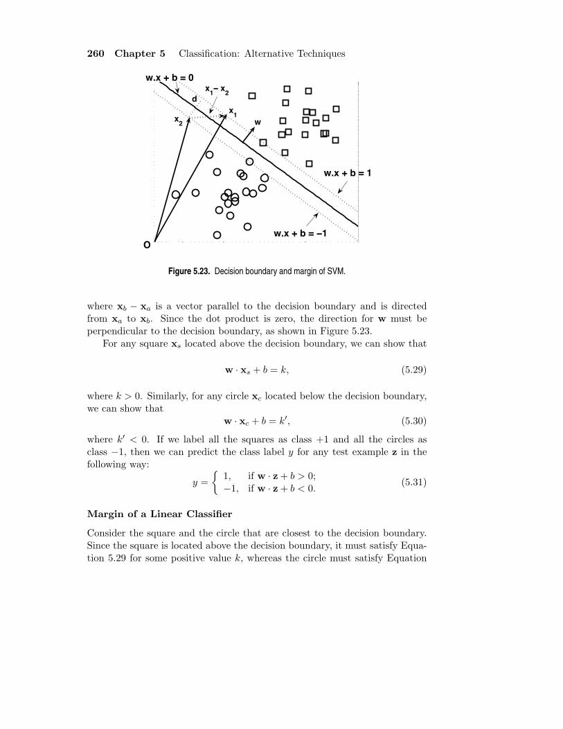
260 Chapter 5 Classification: Alternative Techniques
w
w.x + b = 0
x1
x2
w.x + b = 1
w.x + b = −1
d
O
x1− x
2
Figure 5.23. Decision boundary and margin of SVM.
where xb − xa is a vector parallel to the decision boundary and is directedfrom xa to xb. Since the dot product is zero, the direction for w must beperpendicular to the decision boundary, as shown in Figure 5.23.
For any square xs located above the decision boundary, we can show that
w · xs + b = k, (5.29)
where k > 0. Similarly, for any circle xc located below the decision boundary,we can show that
w · xc + b = k′, (5.30)
where k′ < 0. If we label all the squares as class +1 and all the circles asclass −1, then we can predict the class label y for any test example z in thefollowing way:
y =
{1, if w · z + b > 0;−1, if w · z + b < 0.
(5.31)
Margin of a Linear Classifier
Consider the square and the circle that are closest to the decision boundary.Since the square is located above the decision boundary, it must satisfy Equa-tion 5.29 for some positive value k, whereas the circle must satisfy Equation

5.5 Support Vector Machine (SVM) 261
5.30 for some negative value k′. We can rescale the parameters w and b ofthe decision boundary so that the two parallel hyperplanes bi1 and bi2 can beexpressed as follows:
bi1 : w · x + b = 1, (5.32)
bi2 : w · x + b = −1. (5.33)
The margin of the decision boundary is given by the distance between thesetwo hyperplanes. To compute the margin, let x1 be a data point located onbi1 and x2 be a data point on bi2, as shown in Figure 5.23. Upon substitutingthese points into Equations 5.32 and 5.33, the margin d can be computed bysubtracting the second equation from the first equation:
w · (x1 − x2) = 2
‖w‖ × d = 2
∴ d =2
‖w‖ . (5.34)
Learning a Linear SVM Model
The training phase of SVM involves estimating the parameters w and b of thedecision boundary from the training data. The parameters must be chosen insuch a way that the following two conditions are met:
w · xi + b ≥ 1 if yi = 1,
w · xi + b ≤ −1 if yi = −1. (5.35)
These conditions impose the requirements that all training instances fromclass y = 1 (i.e., the squares) must be located on or above the hyperplanew · x + b = 1, while those instances from class y = −1 (i.e., the circles) mustbe located on or below the hyperplane w · x + b = −1. Both inequalities canbe summarized in a more compact form as follows:
yi(w · xi + b) ≥ 1, i = 1, 2, . . . , N. (5.36)
Although the preceding conditions are also applicable to any linear classi-fiers (including perceptrons), SVM imposes an additional requirement that themargin of its decision boundary must be maximal. Maximizing the margin,however, is equivalent to minimizing the following objective function:
f(w) =‖w‖2
2. (5.37)

262 Chapter 5 Classification: Alternative Techniques
Definition 5.1 (Linear SVM: Separable Case). The learning task in SVMcan be formalized as the following constrained optimization problem:
minw
‖w‖22
subject to yi(w · xi + b) ≥ 1, i = 1, 2, . . . , N.
Since the objective function is quadratic and the constraints are linear inthe parameters w and b, this is known as a convex optimization problem,which can be solved using the standard Lagrange multiplier method. Fol-lowing is a brief sketch of the main ideas for solving the optimization problem.A more detailed discussion is given in Appendix E.
First, we must rewrite the objective function in a form that takes intoaccount the constraints imposed on its solutions. The new objective functionis known as the Lagrangian for the optimization problem:
LP =1
2‖w‖2 −
N∑
i=1
λi
(yi(w · xi + b)− 1
), (5.38)
where the parameters λi are called the Lagrange multipliers. The first term inthe Lagrangian is the same as the original objective function, while the secondterm captures the inequality constraints. To understand why the objectivefunction must be modified, consider the original objective function given inEquation 5.37. It is easy to show that the function is minimized when w = 0, anull vector whose components are all zeros. Such a solution, however, violatesthe constraints given in Definition 5.1 because there is no feasible solutionfor b. The solutions for w and b are infeasible if they violate the inequalityconstraints; i.e., if yi(w ·xi+b)−1 < 0. The Lagrangian given in Equation 5.38incorporates this constraint by subtracting the term from its original objectivefunction. Assuming that λi ≥ 0, it is clear that any infeasible solution mayonly increase the value of the Lagrangian.
To minimize the Lagrangian, we must take the derivative of LP with respectto w and b and set them to zero:
∂Lp
∂w= 0 =⇒ w =
N∑
i=1
λiyixi, (5.39)
∂Lp
∂b= 0 =⇒
N∑
i=1
λiyi = 0. (5.40)

5.5 Support Vector Machine (SVM) 263
Because the Lagrange multipliers are unknown, we still cannot solve for w andb. If Definition 5.1 contains only equality instead of inequality constraints, thenwe can use the N equations from equality constraints along with Equations5.39 and 5.40 to find the feasible solutions for w, b, and λi. Note that theLagrange multipliers for equality constraints are free parameters that can takeany values.
One way to handle the inequality constraints is to transform them into aset of equality constraints. This is possible as long as the Lagrange multipliersare restricted to be non-negative. Such transformation leads to the followingconstraints on the Lagrange multipliers, which are known as the Karush-Kuhn-Tucker (KKT) conditions:
λi ≥ 0, (5.41)
λi
[yi(w · xi + b)− 1
]= 0. (5.42)
At first glance, it may seem that there are as many Lagrange multipli-ers as there are training instances. It turns out that many of the Lagrangemultipliers become zero after applying the constraint given in Equation 5.42.The constraint states that the Lagrange multiplier λi must be zero unless thetraining instance xi satisfies the equation yi(w · xi + b) = 1. Such traininginstance, with λi > 0, lies along the hyperplanes bi1 or bi2 and is known as asupport vector. Training instances that do not reside along these hyperplaneshave λi = 0. Equations 5.39 and 5.42 also suggest that the parameters w andb, which define the decision boundary, depend only on the support vectors.
Solving the preceding optimization problem is still quite a daunting taskbecause it involves a large number of parameters: w, b, and λi. The problemcan be simplified by transforming the Lagrangian into a function of the La-grange multipliers only (this is known as the dual problem). To do this, wefirst substitute Equations 5.39 and 5.40 into Equation 5.38. This will lead tothe following dual formulation of the optimization problem:
LD =N∑
i=1
λi −1
2
∑
i,j
λiλjyiyjxi · xj. (5.43)
The key differences between the dual and primary Lagrangians are as fol-lows:
1. The dual Lagrangian involves only the Lagrange multipliers and thetraining data, while the primary Lagrangian involves the Lagrange mul-tipliers as well as parameters of the decision boundary. Nevertheless, thesolutions for both optimization problems are equivalent.

264 Chapter 5 Classification: Alternative Techniques
2. The quadratic term in Equation 5.43 has a negative sign, which meansthat the original minimization problem involving the primary Lagrangian,LP , has turned into a maximization problem involving the dual La-grangian, LD.
For large data sets, the dual optimization problem can be solved usingnumerical techniques such as quadratic programming, a topic that is beyondthe scope of this book. Once the λi’s are found, we can use Equations 5.39and 5.42 to obtain the feasible solutions for w and b. The decision boundarycan be expressed as follows:
( N∑
i=1
λiyixi · x)
+ b = 0. (5.44)
b is obtained by solving Equation 5.42 for the support vectors. Because the λi’sare calculated numerically and can have numerical errors, the value computedfor b may not be unique. Instead it depends on the support vector used inEquation 5.42. In practice, the average value for b is chosen to be the parameterof the decision boundary.
Example 5.5. Consider the two-dimensional data set shown in Figure 5.24,which contains eight training instances. Using quadratic programming, we cansolve the optimization problem stated in Equation 5.43 to obtain the Lagrangemultiplier λi for each training instance. The Lagrange multipliers are depictedin the last column of the table. Notice that only the first two instances havenon-zero Lagrange multipliers. These instances correspond to the supportvectors for this data set.
Let w = (w1, w2) and b denote the parameters of the decision boundary.Using Equation 5.39, we can solve for w1 and w2 in the following way:
w1 =∑
i
λiyixi1 = 65.5621× 1× 0.3858 + 65.5621×−1× 0.4871 = −6.64.
w2 =∑
i
λiyixi2 = 65.5621× 1× 0.4687 + 65.5621×−1× 0.611 = −9.32.
The bias term b can be computed using Equation 5.42 for each support vector:
b(1) = 1−w · x1 = 1− (−6.64)(0.3858)− (−9.32)(0.4687) = 7.9300.
b(2) = −1−w · x2 = −1− (−6.64)(0.4871)− (−9.32)(0.611) = 7.9289.
Averaging these values, we obtain b = 7.93. The decision boundary corre-sponding to these parameters is shown in Figure 5.24.

5.5 Support Vector Machine (SVM) 265
–6.64 x1 – 9.32 x2 + 7.93 = 0
0 0.2 0.4 0.6 0.8 10
0.3858 0.4871 0.9218 0.7382 0.1763 0.4057 0.9355 0.2146
65.5261 65.5261
0 0 0 0 0 0
0.4687 0.611 0.4103 0.8936 0.0579 0.3529 0.8132 0.0099
1 –1 –1 –1
1 1
–1 1
x2x1 yLagrange Multiplier
x1
x2
1
0.9
0.8
0.7
0.6
0.5
0.4
0.3
0.2
0.1
Figure 5.24. Example of a linearly separable data set.
Once the parameters of the decision boundary are found, a test instance zis classified as follows:
f(z) = sign(w · z + b
)= sign
( N∑
i=1
λiyixi · z + b
).
If f(z) = 1, then the test instance is classified as a positive class; otherwise, itis classified as a negative class.

266 Chapter 5 Classification: Alternative Techniques
5.5.3 Linear SVM: Nonseparable Case
Figure 5.25 shows a data set that is similar to Figure 5.22, except it has twonew examples, P and Q. Although the decision boundary B1 misclassifies thenew examples, while B2 classifies them correctly, this does not mean that B2 isa better decision boundary than B1 because the new examples may correspondto noise in the training data. B1 should still be preferred over B2 because ithas a wider margin, and thus, is less susceptible to overfitting. However, theSVM formulation presented in the previous section constructs only decisionboundaries that are mistake-free. This section examines how the formulationcan be modified to learn a decision boundary that is tolerable to small trainingerrors using a method known as the soft margin approach. More importantly,the method presented in this section allows SVM to construct a linear decisionboundary even in situations where the classes are not linearly separable. Todo this, the learning algorithm in SVM must consider the trade-off betweenthe width of the margin and the number of training errors committed by thelinear decision boundary.
B1
B2b21 b22
b11 b12margin for B1
margin for B2 Q
P
Figure 5.25. Decision boundary of SVM for the nonseparable case.

5.5 Support Vector Machine (SVM) 267
1.2
0.6
0.8
–0.2
0.2
0.4
–0.5
1
0
0 10.5 1.5
X2
X1
w.x + b = –1+ξ
w.x + b = –1
w.x + b = 0
ξ /|w|
P
Figure 5.26. Slack variables for nonseparable data.
While the original objective function given in Equation 5.37 is still appli-cable, the decision boundary B1 no longer satisfies all the constraints givenin Equation 5.36. The inequality constraints must therefore be relaxed to ac-commodate the nonlinearly separable data. This can be done by introducingpositive-valued slack variables (ξ) into the constraints of the optimizationproblem, as shown in the following equations:
w · xi + b ≥ 1− ξi if yi = 1,
w · xi + b ≤ −1 + ξi if yi = −1, (5.45)
where ∀i : ξi > 0.To interpret the meaning of the slack variables ξi, consider the diagram
shown in Figure 5.26. The circle P is one of the instances that violates theconstraints given in Equation 5.35. Let w · x + b = −1 + ξ denote a line thatis parallel to the decision boundary and passes through the point P. It can beshown that the distance between this line and the hyperplane w · x + b = −1is ξ/‖w‖. Thus, ξ provides an estimate of the error of the decision boundaryon the training example P.
In principle, we can apply the same objective function as before and imposethe conditions given in Equation 5.45 to find the decision boundary. However,

268 Chapter 5 Classification: Alternative Techniques
Q
P
Figure 5.27. A decision boundary that has a wide margin but large training error.
since there are no constraints on the number of mistakes the decision boundarycan make, the learning algorithm may find a decision boundary with a verywide margin but misclassifies many of the training examples, as shown inFigure 5.27. To avoid this problem, the objective function must be modifiedto penalize a decision boundary with large values of slack variables. Themodified objective function is given by the following equation:
f(w) =‖w‖2
2+ C(
N∑
i=1
ξi)k,
where C and k are user-specified parameters representing the penalty of mis-classifying the training instances. For the remainder of this section, we assumek = 1 to simplify the problem. The parameter C can be chosen based on themodel’s performance on the validation set.
It follows that the Lagrangian for this constrained optimization problemcan be written as follows:
LP =1
2‖w‖2 + C
N∑
i=1
ξi −N∑
i=1
λi{yi(w · xi + b)− 1 + ξi} −N∑
i=1
µiξi, (5.46)
where the first two terms are the objective function to be minimized, the thirdterm represents the inequality constraints associated with the slack variables,

5.5 Support Vector Machine (SVM) 269
and the last term is the result of the non-negativity requirements on the val-ues of ξi’s. Furthermore, the inequality constraints can be transformed intoequality constraints using the following KKT conditions:
ξi ≥ 0, λi ≥ 0, µi ≥ 0, (5.47)
λi{yi(w · xi + b)− 1 + ξi} = 0, (5.48)
µiξi = 0. (5.49)
Note that the Lagrange multiplier λi given in Equation 5.48 is non-vanishingonly if the training instance resides along the lines w · xi + b = ±1 or hasξi > 0. On the other hand, the Lagrange multipliers µi given in Equation 5.49are zero for any training instances that are misclassified (i.e., having ξi > 0).
Setting the first-order derivative of L with respect to w, b, and ξi to zerowould result in the following equations:
∂L
∂wj= wj −
N∑
i=1
λiyixij = 0 =⇒ wj =N∑
i=1
λiyixij . (5.50)
∂L
∂b= −
N∑
i=1
λiyi = 0 =⇒N∑
i=1
λiyi = 0. (5.51)
∂L
∂ξi= C − λi − µi = 0 =⇒ λi + µi = C. (5.52)
Substituting Equations 5.50, 5.51, and 5.52 into the Lagrangian will pro-duce the following dual Lagrangian:
LD =1
2
∑
i,j
λiλjyiyjxi · xj + C∑
i
ξi
−∑
i
λi{yi(∑
j
λjyjxi · xj + b)− 1 + ξi}
−∑
i
(C − λi)ξi
=
N∑
i=1
λi −1
2
∑
i,j
λiλjyiyjxi · xj, (5.53)
which turns out to be identical to the dual Lagrangian for linearly separabledata (see Equation 5.40 on page 262). Nevertheless, the constraints imposed

270 Chapter 5 Classification: Alternative Techniques
on the Lagrange multipliers λi’s are slightly different those in the linearlyseparable case. In the linearly separable case, the Lagrange multipliers mustbe non-negative, i.e., λi ≥ 0. On the other hand, Equation 5.52 suggests thatλi should not exceed C (since both µi and λi are non-negative). Therefore,the Lagrange multipliers for nonlinearly separable data are restricted to 0 ≤λi ≤ C.
The dual problem can then be solved numerically using quadratic pro-gramming techniques to obtain the Lagrange multipliers λi. These multiplierscan be replaced into Equation 5.50 and the KKT conditions to obtain theparameters of the decision boundary.
5.5.4 Nonlinear SVM
The SVM formulations described in the previous sections construct a linear de-cision boundary to separate the training examples into their respective classes.This section presents a methodology for applying SVM to data sets that havenonlinear decision boundaries. The trick here is to transform the data from itsoriginal coordinate space in x into a new space Φ(x) so that a linear decisionboundary can be used to separate the instances in the transformed space. Af-ter doing the transformation, we can apply the methodology presented in theprevious sections to find a linear decision boundary in the transformed space.
Attribute Transformation
To illustrate how attribute transformation can lead to a linear decision bound-ary, Figure 5.28(a) shows an example of a two-dimensional data set consistingof squares (classified as y = 1) and circles (classified as y = −1). The data setis generated in such a way that all the circles are clustered near the center ofthe diagram and all the squares are distributed farther away from the center.Instances of the data set can be classified using the following equation:
y(x1, x2) =
{1 if
√(x1 − 0.5)2 + (x2 − 0.5)2 > 0.2,
−1 otherwise.(5.54)
The decision boundary for the data can therefore be written as follows:
√(x1 − 0.5)2 + (x2 − 0.5)2 = 0.2,
which can be further simplified into the following quadratic equation:
x21 − x1 + x2
2 − x2 = −0.46.

5.5 Support Vector Machine (SVM) 271
0 0.1 0.2 0.3 0.4 0.5 0.6 0.7 0.8 0.9 1
1
0.9
0.8
0.7
0.6
0.5
0.4
0.3
0.2
0.1
0
X1
X2
(a) Decision boundary in the originaltwo-dimensional space.
–0.25 –0.2 –0.15 –0.1 –0.05 0
–0.25
–0.2
–0.15
–0.1
–0.05
0
X1 – X12
X2
– X
22
(b) Decision boundary in the trans-formed space.
Figure 5.28. Classifying data with a nonlinear decision boundary.
A nonlinear transformation Φ is needed to map the data from its originalfeature space into a new space where the decision boundary becomes linear.Suppose we choose the following transformation:
Φ : (x1, x2) −→ (x21, x
22,√
2x1,√
2x2, 1). (5.55)
In the transformed space, we can find the parameters w = (w0, w1, . . ., w4)such that:
w4x21 + w3x
22 + w2
√2x1 + w1
√2x2 + w0 = 0.
For illustration purposes, let us plot the graph of x22 − x2 versus x2
1 − x1 forthe previously given instances. Figure 5.28(b) shows that in the transformedspace, all the circles are located in the lower right-hand side of the diagram. Alinear decision boundary can therefore be constructed to separate the instancesinto their respective classes.
One potential problem with this approach is that it may suffer from thecurse of dimensionality problem often associated with high-dimensional data.We will show how nonlinear SVM avoids this problem (using a method knownas the kernel trick) later in this section.
Learning a Nonlinear SVM Model
Although the attribute transformation approach seems promising, it raisesseveral implementation issues. First, it is not clear what type of mapping

272 Chapter 5 Classification: Alternative Techniques
function should be used to ensure that a linear decision boundary can beconstructed in the transformed space. One possibility is to transform the datainto an infinite dimensional space, but such a high-dimensional space may notbe that easy to work with. Second, even if the appropriate mapping function isknown, solving the constrained optimization problem in the high-dimensionalfeature space is a computationally expensive task.
To illustrate these issues and examine the ways they can be addressed, letus assume that there is a suitable function, Φ(x), to transform a given dataset. After the transformation, we need to construct a linear decision boundarythat will separate the instances into their respective classes. The linear decisionboundary in the transformed space has the following form: w · Φ(x) + b = 0.
Definition 5.2 (Nonlinear SVM). The learning task for a nonlinear SVMcan be formalized as the following optimization problem:
minw
‖w‖22
subject to yi(w · Φ(xi) + b) ≥ 1, i = 1, 2, . . . , N.
Note the similarity between the learning task of a nonlinear SVM to thatof a linear SVM (see Definition 5.1 on page 262). The main difference is that,instead of using the original attributes x, the learning task is performed on thetransformed attributes Φ(x). Following the approach taken in Sections 5.5.2and 5.5.3 for linear SVM, we may derive the following dual Lagrangian for theconstrained optimization problem:
LD =
n∑
i=1
λi −1
2
∑
i,j
λiλjyiyjΦ(xi) · Φ(xj) (5.56)
Once the λi’s are found using quadratic programming techniques, the param-eters w and b can be derived using the following equations:
w =∑
i
λiyiΦ(xi) (5.57)
λi{yi(∑
j
λjyjΦ(xj) · Φ(xi) + b)− 1} = 0, (5.58)

5.5 Support Vector Machine (SVM) 273
which are analogous to Equations 5.39 and 5.40 for linear SVM. Finally, a testinstance z can be classified using the following equation:
f(z) = sign(w · Φ(z) + b
)= sign
( n∑
i=1
λiyiΦ(xi) · Φ(z) + b
). (5.59)
Except for Equation 5.57, note that the rest of the computations (Equa-tions 5.58 and 5.59) involve calculating the dot product (i.e., similarity) be-tween pairs of vectors in the transformed space, Φ(xi) ·Φ(xj). Such computa-tion can be quite cumbersome and may suffer from the curse of dimensionalityproblem. A breakthrough solution to this problem comes in the form of amethod known as the kernel trick.
Kernel Trick
The dot product is often regarded as a measure of similarity between twoinput vectors. For example, the cosine similarity described in Section 2.4.5on page 73 can be defined as the dot product between two vectors that arenormalized to unit length. Analogously, the dot product Φ(xi) ·Φ(xj) can alsobe regarded as a measure of similarity between two instances, xi and xj , inthe transformed space.
The kernel trick is a method for computing similarity in the transformedspace using the original attribute set. Consider the mapping function Φ givenin Equation 5.55. The dot product between two input vectors u and v in thetransformed space can be written as follows:
Φ(u) · Φ(v) = (u21, u
22,√
2u1,√
2u2, 1) · (v21, v
22,√
2v1,√
2v2, 1)
= u21v
21 + u2
2v22 + 2u1v1 + 2u2v2 + 1
= (u · v + 1)2. (5.60)
This analysis shows that the dot product in the transformed space can beexpressed in terms of a similarity function in the original space:
K(u,v) = Φ(u) · Φ(v) = (u · v + 1)2. (5.61)
The similarity function, K, which is computed in the original attribute space,is known as the kernel function. The kernel trick helps to address someof the concerns about how to implement nonlinear SVM. First, we do nothave to know the exact form of the mapping function Φ because the kernel

274 Chapter 5 Classification: Alternative Techniques
functions used in nonlinear SVM must satisfy a mathematical principle knownas Mercer’s theorem. This principle ensures that the kernel functions canalways be expressed as the dot product between two input vectors in somehigh-dimensional space. The transformed space of the SVM kernels is calleda reproducing kernel Hilbert space (RKHS). Second, computing thedot products using kernel functions is considerably cheaper than using thetransformed attribute set Φ(x). Third, since the computations are performedin the original space, issues associated with the curse of dimensionality problemcan be avoided.
Figure 5.29 shows the nonlinear decision boundary obtained by SVM usingthe polynomial kernel function given in Equation 5.61. A test instance x isclassified according to the following equation:
f(z) = sign(n∑
i=1
λiyiΦ(xi) · Φ(z) + b)
= sign(n∑
i=1
λiyiK(xi, z) + b)
= sign(n∑
i=1
λiyi(xi · z + 1)2 + b), (5.62)
where b is the parameter obtained using Equation 5.58. The decision boundaryobtained by nonlinear SVM is quite close to the true decision boundary shownin Figure 5.28(a).
Mercer’s Theorem
The main requirement for the kernel function used in nonlinear SVM is thatthere must exist a corresponding transformation such that the kernel functioncomputed for a pair of vectors is equivalent to the dot product between thevectors in the transformed space. This requirement can be formally stated inthe form of Mercer’s theorem.
Theorem 5.1 (Mercer’s Theorem). A kernel function K can be expressedas
K(u, v) = Φ(u) · Φ(v)
if and only if, for any function g(x) such that∫
g(x)2dx is finite, then
∫K(x,y) g(x) g(y) dx dy ≥ 0.

5.5 Support Vector Machine (SVM) 275
0 0.1 0.2 0.3 0.4 0.5 0.6 0.7 0.8 0.9 1
1
0.9
0.8
0.7
0.6
0.5
0.4
0.3
0.2
0.1
0
X1
X2
Figure 5.29. Decision boundary produced by a nonlinear SVM with polynomial kernel.
Kernel functions that satisfy Theorem 5.1 are called positive definite kernelfunctions. Examples of such functions are listed below:
K(x,y) = (x · y + 1)p (5.63)
K(x,y) = e−‖x−y‖2/(2σ2) (5.64)
K(x,y) = tanh(kx · y − δ) (5.65)
Example 5.6. Consider the polynomial kernel function given in Equation5.63. Let g(x) be a function that has a finite L2 norm, i.e.,
∫g(x)2dx <∞.
∫(x · y + 1)pg(x)g(y)dxdy
=
∫ p∑
i=0
(p
i
)(x · y)ig(x)g(y)dxdy
=
p∑
i=0
(p
i
)∫ ∑
α1,α2,...
(i
α1α2 . . .
)[(x1y1)
α1(x2y2)α2(x3y3)
α3 . . .
]
g(x1, x2, . . .) g(y1, y2, . . .)dx1dx2 . . . dy1dy2 . . .

276 Chapter 5 Classification: Alternative Techniques
=
p∑
i=0
∑
α1,α2,...
(p
i
)(i
α1α2 . . .
)[∫xα1
1 xα22 . . . g(x1, x2, . . .)dx1dx2 . . .
]2
.
Because the result of the integration is non-negative, the polynomial kernelfunction therefore satisfies Mercer’s theorem.
5.5.5 Characteristics of SVM
SVM has many desirable qualities that make it one of the most widely usedclassification algorithms. Following is a summary of the general characteristicsof SVM:
1. The SVM learning problem can be formulated as a convex optimizationproblem, in which efficient algorithms are available to find the globalminimum of the objective function. Other classification methods, suchas rule-based classifiers and artificial neural networks, employ a greedy-based strategy to search the hypothesis space. Such methods tend tofind only locally optimum solutions.
2. SVM performs capacity control by maximizing the margin of the decisionboundary. Nevertheless, the user must still provide other parameterssuch as the type of kernel function to use and the cost function C forintroducing each slack variable.
3. SVM can be applied to categorical data by introducing dummy variablesfor each categorical attribute value present in the data. For example, ifMarital Status has three values {Single, Married, Divorced}, we canintroduce a binary variable for each of the attribute values.
4. The SVM formulation presented in this chapter is for binary class prob-lems. Some of the methods available to extend SVM to multiclass prob-lems are presented in Section 5.8.
5.6 Ensemble Methods
The classification techniques we have seen so far in this chapter, with the ex-ception of the nearest-neighbor method, predict the class labels of unknownexamples using a single classifier induced from training data. This sectionpresents techniques for improving classification accuracy by aggregating thepredictions of multiple classifiers. These techniques are known as the ensem-ble or classifier combination methods. An ensemble method constructs a

5.6 Ensemble Methods 277
set of base classifiers from training data and performs classification by takinga vote on the predictions made by each base classifier. This section explainswhy ensemble methods tend to perform better than any single classifier andpresents techniques for constructing the classifier ensemble.
5.6.1 Rationale for Ensemble Method
The following example illustrates how an ensemble method can improve aclassifier’s performance.
Example 5.7. Consider an ensemble of twenty-five binary classifiers, each ofwhich has an error rate of ǫ = 0.35. The ensemble classifier predicts the classlabel of a test example by taking a majority vote on the predictions madeby the base classifiers. If the base classifiers are identical, then the ensemblewill misclassify the same examples predicted incorrectly by the base classifiers.Thus, the error rate of the ensemble remains 0.35. On the other hand, if thebase classifiers are independent—i.e., their errors are uncorrelated—then theensemble makes a wrong prediction only if more than half of the base classifierspredict incorrectly. In this case, the error rate of the ensemble classifier is
eensemble =25∑
i=13
(25
i
)ǫi(1− ǫ)25−i = 0.06, (5.66)
which is considerably lower than the error rate of the base classifiers.
Figure 5.30 shows the error rate of an ensemble of twenty-five binary clas-sifiers (eensemble) for different base classifier error rates (ǫ). The diagonal linerepresents the case in which the base classifiers are identical, while the solidline represents the case in which the base classifiers are independent. Observethat the ensemble classifier performs worse than the base classifiers when ǫ islarger than 0.5.
The preceding example illustrates two necessary conditions for an ensem-ble classifier to perform better than a single classifier: (1) the base classifiersshould be independent of each other, and (2) the base classifiers should do bet-ter than a classifier that performs random guessing. In practice, it is difficult toensure total independence among the base classifiers. Nevertheless, improve-ments in classification accuracies have been observed in ensemble methods inwhich the base classifiers are slightly correlated.

278 Chapter 5 Classification: Alternative Techniques
0 0.2 0.4 0.6 0.8 10
0.1
0.2
0.3
0.4
0.5
0.6
0.7
0.8
0.9
1
Base classifier error
Ense
mble
cla
ssifi
er
err
or
Figure 5.30. Comparison between errors of base classifiers and errors of the ensemble classifier.
Original Training data
Step 1:Create Multiple
Data Sets
Step 2:Build Multiple
Classifiers
Step 3:Combine
Classifiers
D
D1 D2 Dt-1 Dt
C1 C2
C*
Ct-1 Ct
....
Figure 5.31. A logical view of the ensemble learning method.
5.6.2 Methods for Constructing an Ensemble Classifier
A logical view of the ensemble method is presented in Figure 5.31. The basicidea is to construct multiple classifiers from the original data and then aggre-gate their predictions when classifying unknown examples. The ensemble ofclassifiers can be constructed in many ways:

5.6 Ensemble Methods 279
1. By manipulating the training set. In this approach, multiple train-ing sets are created by resampling the original data according to somesampling distribution. The sampling distribution determines how likelyit is that an example will be selected for training, and it may vary fromone trial to another. A classifier is then built from each training set usinga particular learning algorithm. Bagging and boosting are two exam-ples of ensemble methods that manipulate their training sets. Thesemethods are described in further detail in Sections 5.6.4 and 5.6.5.
2. By manipulating the input features. In this approach, a subsetof input features is chosen to form each training set. The subset canbe either chosen randomly or based on the recommendation of domainexperts. Some studies have shown that this approach works very wellwith data sets that contain highly redundant features. Random forest,which is described in Section 5.6.6, is an ensemble method that manip-ulates its input features and uses decision trees as its base classifiers.
3. By manipulating the class labels. This method can be used when thenumber of classes is sufficiently large. The training data is transformedinto a binary class problem by randomly partitioning the class labelsinto two disjoint subsets, A0 and A1. Training examples whose classlabel belongs to the subset A0 are assigned to class 0, while those thatbelong to the subset A1 are assigned to class 1. The relabeled examplesare then used to train a base classifier. By repeating the class-relabelingand model-building steps multiple times, an ensemble of base classifiersis obtained. When a test example is presented, each base classifier Ci isused to predict its class label. If the test example is predicted as class0, then all the classes that belong to A0 will receive a vote. Conversely,if it is predicted to be class 1, then all the classes that belong to A1
will receive a vote. The votes are tallied and the class that receives thehighest vote is assigned to the test example. An example of this approachis the error-correcting output coding method described on page 307.
4. By manipulating the learning algorithm. Many learning algo-rithms can be manipulated in such a way that applying the algorithmseveral times on the same training data may result in different models.For example, an artificial neural network can produce different mod-els by changing its network topology or the initial weights of the linksbetween neurons. Similarly, an ensemble of decision trees can be con-structed by injecting randomness into the tree-growing procedure. For

280 Chapter 5 Classification: Alternative Techniques
example, instead of choosing the best splitting attribute at each node,we can randomly choose one of the top k attributes for splitting.
The first three approaches are generic methods that are applicable to anyclassifiers, whereas the fourth approach depends on the type of classifier used.The base classifiers for most of these approaches can be generated sequentially(one after another) or in parallel (all at once). Algorithm 5.5 shows the stepsneeded to build an ensemble classifier in a sequential manner. The first stepis to create a training set from the original data D. Depending on the typeof ensemble method used, the training sets are either identical to or slightmodifications of D. The size of the training set is often kept the same as theoriginal data, but the distribution of examples may not be identical; i.e., someexamples may appear multiple times in the training set, while others may notappear even once. A base classifier Ci is then constructed from each trainingset Di. Ensemble methods work better with unstable classifiers, i.e., baseclassifiers that are sensitive to minor perturbations in the training set. Ex-amples of unstable classifiers include decision trees, rule-based classifiers, andartificial neural networks. As will be discussed in Section 5.6.3, the variabilityamong training examples is one of the primary sources of errors in a classifier.By aggregating the base classifiers built from different training sets, this mayhelp to reduce such types of errors.
Finally, a test example x is classified by combining the predictions madeby the base classifiers Ci(x):
C∗(x) = V ote(C1(x), C2(x), . . . , Ck(x)).
The class can be obtained by taking a majority vote on the individual predic-tions or by weighting each prediction with the accuracy of the base classifier.
Algorithm 5.5 General procedure for ensemble method.1: Let D denote the original training data, k denote the number of base classifiers,
and T be the test data.2: for i = 1 to k do3: Create training set, Di from D.4: Build a base classifier Ci from Di.5: end for6: for each test record x ∈ T do7: C∗(x) = V ote(C1(x), C2(x), . . . , Ck(x))8: end for

5.6 Ensemble Methods 281
5.6.3 Bias-Variance Decomposition
Bias-variance decomposition is a formal method for analyzing the predictionerror of a predictive model. The following example gives an intuitive explana-tion for this method.
Figure 5.32 shows the trajectories of a projectile launched at a particularangle. Suppose the projectile hits the floor surface at some location x, at adistance d away from the target position t. Depending on the force appliedto the projectile, the observed distance may vary from one trial to another.The observed distance can be decomposed into several components. The firstcomponent, which is known as bias, measures the average distance betweenthe target position and the location where the projectile hits the floor. Theamount of bias depends on the angle of the projectile launcher. The secondcomponent, which is known as variance, measures the deviation between xand the average position x where the projectile hits the floor. The variancecan be explained as a result of changes in the amount of force applied to theprojectile. Finally, if the target is not stationary, then the observed distanceis also affected by changes in the location of the target. This is considered thenoise component associated with variability in the target position. Puttingthese components together, the average distance can be expressed as:
df,θ(y, t) = Biasθ + Variancef + Noiset, (5.67)
where f refers to the amount of force applied and θ is the angle of the launcher.The task of predicting the class label of a given example can be analyzed
using the same approach. For a given classifier, some predictions may turn outto be correct, while others may be completely off the mark. We can decomposethe expected error of a classifier as a sum of the three terms given in Equation5.67, where expected error is the probability that the classifier misclassifies a
Target, t
ʻVarianceʼ ʻNoiseʼ
ʻBiasʼ
y
Figure 5.32. Bias-variance decomposition.

282 Chapter 5 Classification: Alternative Techniques
given example. The remainder of this section examines the meaning of bias,variance, and noise in the context of classification.
A classifier is usually trained to minimize its training error. However, tobe useful, the classifier must be able to make an informed guess about theclass labels of examples it has never seen before. This requires the classifier togeneralize its decision boundary to regions where there are no training exam-ples available—a decision that depends on the design choice of the classifier.For example, a key design issue in decision tree induction is the amount ofpruning needed to obtain a tree with low expected error. Figure 5.33 showstwo decision trees, T1 and T2, that are generated from the same training data,but have different complexities. T2 is obtained by pruning T1 until a tree withmaximum depth of two is obtained. T1, on the other hand, performs very littlepruning on its decision tree. These design choices will introduce a bias intothe classifier that is analogous to the bias of the projectile launcher describedin the previous example. In general, the stronger the assumptions made bya classifier about the nature of its decision boundary, the larger the classi-fier’s bias will be. T2 therefore has a larger bias because it makes strongerassumptions about its decision boundary (which is reflected by the size of thetree) compared to T1. Other design choices that may introduce a bias into aclassifier include the network topology of an artificial neural network and thenumber of neighbors considered by a nearest-neighbor classifier.
The expected error of a classifier is also affected by variability in the train-ing data because different compositions of the training set may lead to differ-ent decision boundaries. This is analogous to the variance in x when differentamounts of force are applied to the projectile. The last component of the ex-pected error is associated with the intrinsic noise in the target class. The targetclass for some domains can be non-deterministic; i.e., instances with the sameattribute values can have different class labels. Such errors are unavoidableeven when the true decision boundary is known.
The amount of bias and variance contributing to the expected error dependon the type of classifier used. Figure 5.34 compares the decision boundariesproduced by a decision tree and a 1-nearest neighbor classifier. For eachclassifier, we plot the decision boundary obtained by “averaging” the modelsinduced from 100 training sets, each containing 100 examples. The true deci-sion boundary from which the data is generated is also plotted using a dashedline. The difference between the true decision boundary and the “averaged”decision boundary reflects the bias of the classifier. After averaging the mod-els, observe that the difference between the true decision boundary and thedecision boundary produced by the 1-nearest neighbor classifier is smaller than

5.6 Ensemble Methods 283
x2 < 1.94
x2 < 1.94
x2 < 9.25x2 < 7.45
x1 < –1.24
x1 < –1.24
x1 < 11.00
x1 < 11.00
x1 < 1.58
(a) Decision tree T1
(b) Decision tree T2
15
10
5
0
–5–5 0 5 10 15
15
10
5
0
–5–5 0 5 10 15
Figure 5.33. Two decision trees with different complexities induced from the same training data.
the observed difference for a decision tree classifier. This result suggests thatthe bias of a 1-nearest neighbor classifier is lower than the bias of a decisiontree classifier.
On the other hand, the 1-nearest neighbor classifier is more sensitive tothe composition of its training examples. If we examine the models inducedfrom different training sets, there is more variability in the decision boundaryof a 1-nearest neighbor classifier than a decision tree classifier. Therefore, thedecision boundary of a decision tree classifier has a lower variance than the1-nearest neighbor classifier.
5.6.4 Bagging
Bagging, which is also known as bootstrap aggregating, is a technique thatrepeatedly samples (with replacement) from a data set according to a uniformprobability distribution. Each bootstrap sample has the same size as the origi-nal data. Because the sampling is done with replacement, some instances mayappear several times in the same training set, while others may be omittedfrom the training set. On average, a bootstrap sample Di contains approxi-
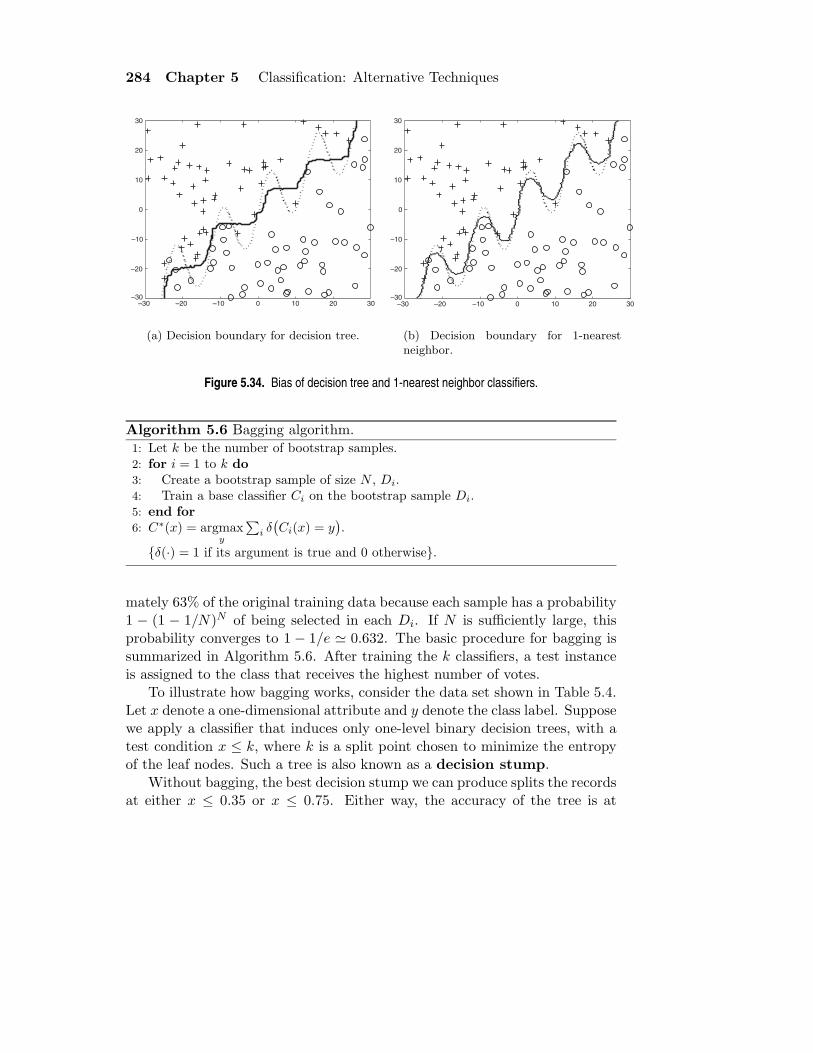
284 Chapter 5 Classification: Alternative Techniques
–30 –20 –10 0 10 20 30–30
–20
–10
0
10
20
30
(a) Decision boundary for decision tree.
–30 –20 –10 0 10 20 30–30
–20
–10
0
10
20
30
(b) Decision boundary for 1-nearestneighbor.
Figure 5.34. Bias of decision tree and 1-nearest neighbor classifiers.
Algorithm 5.6 Bagging algorithm.1: Let k be the number of bootstrap samples.2: for i = 1 to k do3: Create a bootstrap sample of size N , Di.4: Train a base classifier Ci on the bootstrap sample Di.5: end for6: C∗(x) = argmax
y
∑i δ(Ci(x) = y
).
{δ(·) = 1 if its argument is true and 0 otherwise}.
mately 63% of the original training data because each sample has a probability1 − (1 − 1/N)N of being selected in each Di. If N is sufficiently large, thisprobability converges to 1 − 1/e ≃ 0.632. The basic procedure for bagging issummarized in Algorithm 5.6. After training the k classifiers, a test instanceis assigned to the class that receives the highest number of votes.
To illustrate how bagging works, consider the data set shown in Table 5.4.Let x denote a one-dimensional attribute and y denote the class label. Supposewe apply a classifier that induces only one-level binary decision trees, with atest condition x ≤ k, where k is a split point chosen to minimize the entropyof the leaf nodes. Such a tree is also known as a decision stump.
Without bagging, the best decision stump we can produce splits the recordsat either x ≤ 0.35 or x ≤ 0.75. Either way, the accuracy of the tree is at

5.6 Ensemble Methods 285
Table 5.4. Example of data set used to construct an ensemble of bagging classifiers.
x 0.1 0.2 0.3 0.4 0.5 0.6 0.7 0.8 0.9 1
y 1 1 1 −1 −1 −1 −1 1 1 1
most 70%. Suppose we apply the bagging procedure on the data set usingten bootstrap samples. The examples chosen for training in each bagginground are shown in Figure 5.35. On the right-hand side of each table, we alsoillustrate the decision boundary produced by the classifier.
We classify the entire data set given in Table 5.4 by taking a majorityvote among the predictions made by each base classifier. The results of thepredictions are shown in Figure 5.36. Since the class labels are either −1 or+1, taking the majority vote is equivalent to summing up the predicted valuesof y and examining the sign of the resulting sum (refer to the second to lastrow in Figure 5.36). Notice that the ensemble classifier perfectly classifies allten examples in the original data.
The preceding example illustrates another advantage of using ensemblemethods in terms of enhancing the representation of the target function. Eventhough each base classifier is a decision stump, combining the classifiers canlead to a decision tree of depth 2.
Bagging improves generalization error by reducing the variance of the baseclassifiers. The performance of bagging depends on the stability of the baseclassifier. If a base classifier is unstable, bagging helps to reduce the errorsassociated with random fluctuations in the training data. If a base classifieris stable, i.e., robust to minor perturbations in the training set, then theerror of the ensemble is primarily caused by bias in the base classifier. Inthis situation, bagging may not be able to improve the performance of thebase classifiers significantly. It may even degrade the classifier’s performancebecause the effective size of each training set is about 37% smaller than theoriginal data.
Finally, since every sample has an equal probability of being selected, bag-ging does not focus on any particular instance of the training data. It istherefore less susceptible to model overfitting when applied to noisy data.
5.6.5 Boosting
Boosting is an iterative procedure used to adaptively change the distributionof training examples so that the base classifiers will focus on examples thatare hard to classify. Unlike bagging, boosting assigns a weight to each training

286 Chapter 5 Classification: Alternative Techniques
x <= 0.35 ==> y = 1
x > 0.35 ==> y = -1
x <= 0.65 ==> y = 1
x > 0.65 ==> y = 1
x <= 0.35 ==> y = 1
x > 0.35 ==> y = -1
x <= 0.3 ==> y = 1
x > 0.3 ==> y = -1
x <= 0.35 ==> y = 1
x > 0.35 ==> y = -1
x <= 0.75 ==> y = -1
x > 0.75 ==> y = 1
x <= 0.75 ==> y = -1
x > 0.75 ==> y = 1
x <= 0.75 ==> y = -1
x > 0.75 ==> y = 1
x <= 0.75 ==> y = -1
x > 0.75 ==> y = 1
x <= 0.05 ==> y = -1
x > 0.05 ==> y = 1
Bagging Round 1:
x 0.1 0.2 0.2 0.3 0.4 0.4 0.5 0.6 0.9 0.9y 1 1 1 1 -1 -1 -1 -1 1 1
Bagging Round 2:
x 0.1 0.2 0.3 0.4 0.5 0.8 0.9 1 1 1y 1 1 1 -1 -1 11 1 1 1
Bagging Round 3:
x 0.1 0.2 0.3 0.4 0.4 0.5 0.7 0.7 0.8 0.9y 1 1 1 -1 -1 -1 -1 -1 1 1
Bagging Round 4:
x 0.1 0.1 0.2 0.4 0.4 0.5 0.5 0.7 0.8 0.9y 1 1 1 -1 -1 -1 -1 -1 1 1
Bagging Round 5:
x 0.1 0.1 0.2 0.5 0.6 0.6 0.6 1 1 1y 1 1 1 -1 -1 -1 -1 1 1 1
Bagging Round 6:
x 0.2 0.4 0.5 0.6 0.7 0.7 0.7 0.8 0.9 1y 1 -1 -1 -1 -1 -1 -1 1 1 1
Bagging Round 7:
x 0.1 0.4 0.4 0.6 0.7 0.8 0.9 0.9 0.9 1y 1 -1 -1 -1 -1 1 1 1 1 1
Bagging Round 8:
x 0.1 0.2 0.5 0.5 0.5 0.7 0.7 0.8 0.9 1y 1 1 -1 -1 -1 -1 -1 1 1 1
Bagging Round 9:
x 0.1 0.3 0.4 0.4 0.6 0.7 0.7 0.8 1 1y 1 1 -1 -1 -1 -1 -1 1 1 1
Bagging Round 10:
x 0.1 0.1 0.1 0.1 0.3 0.3 0.8 0.8 0.9 0.9y 1 1 1 1 1 1 1 1 1 1
Figure 5.35. Example of bagging.
example and may adaptively change the weight at the end of each boostinground. The weights assigned to the training examples can be used in thefollowing ways:
1. They can be used as a sampling distribution to draw a set of bootstrapsamples from the original data.
2. They can be used by the base classifier to learn a model that is biasedtoward higher-weight examples.

5.6 Ensemble Methods 287
Round x=0.1 x=0.2 x=0.3 x=0.4 x=0.5 x=0.6 x=0.7 x=0.8 x=0.9 x=1.0
1 1 1 1 -1 -1 -1 -1 -1 -1 -1
2 1 1 1 1 1 1 1 1 1 1
3 1 1 1 -1 -1 -1 -1 -1 -1 -1
4 1 1 1 -1 -1 -1 -1 -1 -1 -1
5 1 1 1 -1 -1 -1 -1 -1 -1 -1
6 -1 -1 -1 -1 -1 -1 -1 1 1 1
7 -1 -1 -1 -1 -1 -1 -1 1 1 1
8 -1 -1 -1 -1 -1 -1 -1 1 1 1
9 -1 -1 -1 -1 -1 -1 -1 1 1 1
10 1 1 1 1 1 1 1 1 1 1
Sum 2 2 2 -6 -6 -6 -6 2 2 2
Sign 1 1 1 -1 -1 -1 -1 1 1 1
True Class 1 1 1 -1 -1 -1 -1 1 1 1
Figure 5.36. Example of combining classifiers constructed using the bagging approach.
This section describes an algorithm that uses weights of examples to de-termine the sampling distribution of its training set. Initially, the examplesare assigned equal weights, 1/N , so that they are equally likely to be chosenfor training. A sample is drawn according to the sampling distribution of thetraining examples to obtain a new training set. Next, a classifier is inducedfrom the training set and used to classify all the examples in the original data.The weights of the training examples are updated at the end of each boost-ing round. Examples that are classified incorrectly will have their weightsincreased, while those that are classified correctly will have their weights de-creased. This forces the classifier to focus on examples that are difficult toclassify in subsequent iterations.
The following table shows the examples chosen during each boosting round.
Boosting (Round 1): 7 3 2 8 7 9 4 10 6 3
Boosting (Round 2): 5 4 9 4 2 5 1 7 4 2
Boosting (Round 3): 4 4 8 10 4 5 4 6 3 4
Initially, all the examples are assigned the same weights. However, some ex-amples may be chosen more than once, e.g., examples 3 and 7, because thesampling is done with replacement. A classifier built from the data is thenused to classify all the examples. Suppose example 4 is difficult to classify.The weight for this example will be increased in future iterations as it getsmisclassified repeatedly. Meanwhile, examples that were not chosen in the pre-

288 Chapter 5 Classification: Alternative Techniques
vious round, e.g., examples 1 and 5, also have a better chance of being selectedin the next round since their predictions in the previous round were likely tobe wrong. As the boosting rounds proceed, examples that are the hardest toclassify tend to become even more prevalent. The final ensemble is obtainedby aggregating the base classifiers obtained from each boosting round.
Over the years, several implementations of the boosting algorithm havebeen developed. These algorithms differ in terms of (1) how the weights ofthe training examples are updated at the end of each boosting round, and (2)how the predictions made by each classifier are combined. An implementationcalled AdaBoost is explored in the next section.
AdaBoost
Let {(xj , yj) | j = 1, 2, . . . , N} denote a set of N training examples. In theAdaBoost algorithm, the importance of a base classifier Ci depends on its errorrate, which is defined as
ǫi =1
N
[ N∑
j=1
wj I
(Ci(xj) 6= yj
)], (5.68)
where I(p) = 1 if the predicate p is true, and 0 otherwise. The importance ofa classifier Ci is given by the following parameter,
αi =1
2ln
(1− ǫi
ǫi
).
Note that αi has a large positive value if the error rate is close to 0 and a largenegative value if the error rate is close to 1, as shown in Figure 5.37.
The αi parameter is also used to update the weight of the training ex-
amples. To illustrate, let w(j)i denote the weight assigned to example (xi, yi)
during the jth boosting round. The weight update mechanism for AdaBoostis given by the equation:
w(j+1)i =
w(j)i
Zj×{
exp−αj if Cj(xi) = yi
expαj if Cj(xi) 6= yi
, (5.69)
where Zj is the normalization factor used to ensure that∑
i w(j+1)i = 1. The
weight update formula given in Equation 5.69 increases the weights of incor-rectly classified examples and decreases the weights of those classified correctly.

5.6 Ensemble Methods 289
0 0.2 0.4 0.6 0.8 1–5
–4
–3
–2
–1
0
1
2
3
4
5
ε
In (
(1 –
ε)/
ε)
Figure 5.37. Plot of α as a function of training error ǫ.
Instead of using a majority voting scheme, the prediction made by eachclassifier Cj is weighted according to αj . This approach allows AdaBoost topenalize models that have poor accuracy, e.g., those generated at the earlierboosting rounds. In addition, if any intermediate rounds produce an errorrate higher than 50%, the weights are reverted back to their original uniformvalues, wi = 1/N , and the resampling procedure is repeated. The AdaBoostalgorithm is summarized in Algorithm 5.7.
Let us examine how the boosting approach works on the data set shownin Table 5.4. Initially, all the examples have identical weights. After threeboosting rounds, the examples chosen for training are shown in Figure 5.38(a).The weights for each example are updated at the end of each boosting roundusing Equation 5.69.
Without boosting, the accuracy of the decision stump is, at best, 70%.With AdaBoost, the results of the predictions are given in Figure 5.39(b).The final prediction of the ensemble classifier is obtained by taking a weightedaverage of the predictions made by each base classifier, which is shown in thelast row of Figure 5.39(b). Notice that AdaBoost perfectly classifies all theexamples in the training data.
An important analytical result of boosting shows that the training error ofthe ensemble is bounded by the following expression:
eensemble ≤∏
i
[√ǫi(1− ǫi)
], (5.70)

290 Chapter 5 Classification: Alternative Techniques
Algorithm 5.7 AdaBoost algorithm.
1: w = {wj = 1/N | j = 1, 2, . . . , N}. {Initialize the weights for all N examples.}2: Let k be the number of boosting rounds.3: for i = 1 to k do4: Create training set Di by sampling (with replacement) from D according to w.5: Train a base classifier Ci on Di.6: Apply Ci to all examples in the original training set, D.7: ǫi = 1
N
[∑j wj δ
(Ci(xj) 6= yj
)]{Calculate the weighted error.}
8: if ǫi > 0.5 then9: w = {wj = 1/N | j = 1, 2, . . . , N}. {Reset the weights for all N examples.}
10: Go back to Step 4.11: end if12: αi = 1
2 ln 1−ǫi
ǫi.
13: Update the weight of each example according to Equation 5.69.14: end for15: C∗(x) = argmax
y
∑Tj=1 αjδ(Cj(x) = y)
).
where ǫi is the error rate of each base classifier i. If the error rate of the baseclassifier is less than 50%, we can write ǫi = 0.5− γi, where γi measures howmuch better the classifier is than random guessing. The bound on the trainingerror of the ensemble becomes
eensemble ≤∏
i
√1− 4γ2
i ≤ exp
(− 2
∑
i
γ2i
). (5.71)
If γi < γ∗ for all i’s, then the training error of the ensemble decreases expo-nentially, which leads to the fast convergence of the algorithm. Nevertheless,because of its tendency to focus on training examples that are wrongly classi-fied, the boosting technique can be quite susceptible to overfitting.
5.6.6 Random Forests
Random forest is a class of ensemble methods specifically designed for decisiontree classifiers. It combines the predictions made by multiple decision trees,where each tree is generated based on the values of an independent set ofrandom vectors, as shown in Figure 5.40. The random vectors are generatedfrom a fixed probability distribution, unlike the adaptive approach used inAdaBoost, where the probability distribution is varied to focus on examplesthat are hard to classify. Bagging using decision trees is a special case ofrandom forests, where randomness is injected into the model-building process

5.6 Ensemble Methods 291
Boosting Round 1:
x 0.1 0.4 0.5 0.6 0.6 0.7 0.7 0.7 0.8 1
y 1 -1 -1 -1 -1 -1 -1 -1 1 1
Boosting Round 2:
x 0.1 0.1 0.2 0.2 0.2 0.2 0.3 0.3 0.3 0.3
y 1 1 1 1 1 1 1 1 1 1
Boosting Round 3:
x 0.2 0.2 0.4 0.4 0.4 0.4 0.5 0.6 0.6 0.7
y 1 1 -1 -1 -1 -1 -1 -1 -1 -1
Round x=0.1 x=0.2 x=0.3 x=0.4 x=0.5 x=0.6 x=0.7 x=0.8 x=0.9 x=1.0
1 0.1 0.1 0.1 0.1 0.1 0.1 0.1 0.1 0.1 0.1
2 0.311 0.311 0.311 0.01 0.01 0.01 0.01 0.01 0.01 0.01
3 0.029 0.029 0.029 0.228 0.228 0.228 0.228 0.009 0.009 0.009
(b) Weights of training records
(a) Training records chosen during boosting
Figure 5.38. Example of boosting.
by randomly choosing N samples, with replacement, from the original trainingset. Bagging also uses the same uniform probability distribution to generateits bootstrapped samples throughout the entire model-building process.
It was theoretically proven that the upper bound for generalization errorof random forests converges to the following expression, when the number oftrees is sufficiently large.
Generalization error ≤ ρ(1− s2)
s2, (5.72)
where ρ is the average correlation among the trees and s is a quantity thatmeasures the “strength” of the tree classifiers. The strength of a set of classi-fiers refers to the average performance of the classifiers, where performance ismeasured probabilistically in terms of the classifier’s margin:
margin, M(X, Y ) = P (Yθ = Y )−maxZ 6=Y
P (Yθ = Z), (5.73)
where Yθ is the predicted class of X according to a classifier built from somerandom vector θ. The higher the margin is, the more likely it is that the

292 Chapter 5 Classification: Alternative Techniques
(a)
(b)
Round Split Point Left Class Right Class
1 0.75 -1 1 1.738
2 0.05 1 1 2.7784
3 0.3 1 -1 4.1195
Round x=0.1 x=0.2 x=0.3 x=0.4 x=0.5 x=0.6 x=0.7 x=0.8 x=0.9 x=1.0
1 -1 -1 -1 -1 -1 -1 -1 1 1 1
2 1 1 1 1 1 1 1 1 1 1
3 1 1 1 -1 -1 -1 -1 -1 -1 -1
Sum 5.16 5.16 5.16 -3.08 -3.08 -3.08 -3.08 0.397 0.397 0.397
Sign 1 1 1 -1 -1 -1 -1 1 1 1
α
Figure 5.39. Example of combining classifiers constructed using the AdaBoost approach.
Step 1:Create random
vectors
Step 2:Use random
vector tobuild multipledecision trees
Step 3:Combine
decision trees
D
D1 D2 Dt-1 Dt
T1 T2 T1–1 T1
T*
...
OriginalTraining data
Randomize
Figure 5.40. Random forests.
classifier correctly predicts a given example X. Equation 5.72 is quite intuitive;as the trees become more correlated or the strength of the ensemble decreases,the generalization error bound tends to increase. Randomization helps toreduce the correlation among decision trees so that the generalization error ofthe ensemble can be improved.

5.6 Ensemble Methods 293
Each decision tree uses a random vector that is generated from some fixedprobability distribution. A random vector can be incorporated into the tree-growing process in many ways. The first approach is to randomly select Finput features to split at each node of the decision tree. As a result, instead ofexamining all the available features, the decision to split a node is determinedfrom these selected F features. The tree is then grown to its entirety withoutany pruning. This may help reduce the bias present in the resulting tree.Once the trees have been constructed, the predictions are combined using amajority voting scheme. This approach is known as Forest-RI, where RI refersto random input selection. To increase randomness, bagging can also be usedto generate bootstrap samples for Forest-RI. The strength and correlation ofrandom forests may depend on the size of F . If F is sufficiently small, thenthe trees tend to become less correlated. On the other hand, the strength ofthe tree classifier tends to improve with a larger number of features, F . Asa tradeoff, the number of features is commonly chosen to be F = log2 d + 1,where d is the number of input features. Since only a subset of the featuresneeds to be examined at each node, this approach helps to significantly reducethe runtime of the algorithm.
If the number of original features d is too small, then it is difficult to choosean independent set of random features for building the decision trees. Oneway to increase the feature space is to create linear combinations of the inputfeatures. Specifically, at each node, a new feature is generated by randomlyselecting L of the input features. The input features are linearly combinedusing coefficients generated from a uniform distribution in the range of [−1,1]. At each node, F of such randomly combined new features are generated,and the best of them is subsequently selected to split the node. This approachis known as Forest-RC.
A third approach for generating the random trees is to randomly selectone of the F best splits at each node of the decision tree. This approach maypotentially generate trees that are more correlated than Forest-RI and Forest-RC, unless F is sufficiently large. It also does not have the runtime savings ofForest-RI and Forest-RC because the algorithm must examine all the splittingfeatures at each node of the decision tree.
It has been shown empirically that the classification accuracies of randomforests are quite comparable to the AdaBoost algorithm. It is also more robustto noise and runs much faster than the AdaBoost algorithm. The classificationaccuracies of various ensemble algorithms are compared in the next section.

294 Chapter 5 Classification: Alternative Techniques
Table 5.5. Comparing the accuracy of a decision tree classifier against three ensemble methods.
Data Set Number of Decision Bagging Boosting RF(Attributes, Classes, Tree (%) (%) (%) (%)
Records)
Anneal (39, 6, 898) 92.09 94.43 95.43 95.43Australia (15, 2, 690) 85.51 87.10 85.22 85.80Auto (26, 7, 205) 81.95 85.37 85.37 84.39Breast (11, 2, 699) 95.14 96.42 97.28 96.14Cleve (14, 2, 303) 76.24 81.52 82.18 82.18Credit (16, 2, 690) 85.8 86.23 86.09 85.8Diabetes (9, 2, 768) 72.40 76.30 73.18 75.13German (21, 2, 1000) 70.90 73.40 73.00 74.5Glass (10, 7, 214) 67.29 76.17 77.57 78.04Heart (14, 2, 270) 80.00 81.48 80.74 83.33Hepatitis (20, 2, 155) 81.94 81.29 83.87 83.23Horse (23, 2, 368) 85.33 85.87 81.25 85.33Ionosphere (35, 2, 351) 89.17 92.02 93.73 93.45Iris (5, 3, 150) 94.67 94.67 94.00 93.33Labor (17, 2, 57) 78.95 84.21 89.47 84.21Led7 (8, 10, 3200) 73.34 73.66 73.34 73.06Lymphography (19, 4, 148) 77.03 79.05 85.14 82.43Pima (9, 2, 768) 74.35 76.69 73.44 77.60Sonar (61, 2, 208) 78.85 78.85 84.62 85.58Tic-tac-toe (10, 2, 958) 83.72 93.84 98.54 95.82Vehicle (19, 4, 846) 71.04 74.11 78.25 74.94Waveform (22, 3, 5000) 76.44 83.30 83.90 84.04Wine (14, 3, 178) 94.38 96.07 97.75 97.75Zoo (17, 7, 101) 93.07 93.07 95.05 97.03
5.6.7 Empirical Comparison among Ensemble Methods
Table 5.5 shows the empirical results obtained when comparing the perfor-mance of a decision tree classifier against bagging, boosting, and random for-est. The base classifiers used in each ensemble method consist of fifty decisiontrees. The classification accuracies reported in this table are obtained fromten-fold cross-validation. Notice that the ensemble classifiers generally out-perform a single decision tree classifier on many of the data sets.
5.7 Class Imbalance Problem
Data sets with imbalanced class distributions are quite common in many realapplications. For example, an automated inspection system that monitorsproducts that come off a manufacturing assembly line may find that the num-

5.7 Class Imbalance Problem 295
ber of defective products is significantly fewer than that of non-defective prod-ucts. Similarly, in credit card fraud detection, fraudulent transactions areoutnumbered by legitimate transactions. In both of these examples, there isa disproportionate number of instances that belong to different classes. Thedegree of imbalance varies from one application to another—a manufacturingplant operating under the six sigma principle may discover four defects in amillion products shipped to their customers, while the amount of credit cardfraud may be of the order of 1 in 100. Despite their infrequent occurrences,a correct classification of the rare class in these applications often has greatervalue than a correct classification of the majority class. However, because theclass distribution is imbalanced, this presents a number of problems to existingclassification algorithms.
The accuracy measure, which is used extensively to compare the perfor-mance of classifiers, may not be well suited for evaluating models derived fromimbalanced data sets. For example, if 1% of the credit card transactions arefraudulent, then a model that predicts every transaction as legitimate has anaccuracy of 99% even though it fails to detect any of the fraudulent activities.Additionally, measures that are used to guide the learning algorithm (e.g., in-formation gain for decision tree induction) may need to be modified to focuson the rare class.
Detecting instances of the rare class is akin to finding a needle in a haystack.Because their instances occur infrequently, models that describe the rare classtend to be highly specialized. For example, in a rule-based classifier, therules extracted for the rare class typically involve a large number of attributesand cannot be easily simplified into more general rules with broader coverage(unlike the rules for the majority class). Such models are also susceptibleto the presence of noise in training data. As a result, many of the existingclassification algorithms may not effectively detect instances of the rare class.
This section presents some of the methods developed for handling the classimbalance problem. First, alternative metrics besides accuracy are introduced,along with a graphical method called ROC analysis. We then describe howcost-sensitive learning and sampling-based methods may be used to improvethe detection of rare classes.
5.7.1 Alternative Metrics
Since the accuracy measure treats every class as equally important, it maynot be suitable for analyzing imbalanced data sets, where the rare class isconsidered more interesting than the majority class. For binary classification,the rare class is often denoted as the positive class, while the majority class is

296 Chapter 5 Classification: Alternative Techniques
Table 5.6. A confusion matrix for a binary classification problem in which the classes are not equally
important.
Predicted Class
+ −Actual + f++ (TP) f+− (FN)
Class − f−+ (FP) f−− (TN)
denoted as the negative class. A confusion matrix that summarizes the numberof instances predicted correctly or incorrectly by a classification model is shownin Table 5.6.
The following terminology is often used when referring to the counts tab-ulated in a confusion matrix:
• True positive (TP) or f++, which corresponds to the number of positiveexamples correctly predicted by the classification model.
• False negative (FN) or f+−, which corresponds to the number of positiveexamples wrongly predicted as negative by the classification model.
• False positive (FP) or f−+, which corresponds to the number of negativeexamples wrongly predicted as positive by the classification model.
• True negative (TN) or f−−, which corresponds to the number of negativeexamples correctly predicted by the classification model.
The counts in a confusion matrix can also be expressed in terms of percentages.The true positive rate (TPR) or sensitivity is defined as the fraction ofpositive examples predicted correctly by the model, i.e.,
TPR = TP/(TP + FN).
Similarly, the true negative rate (TNR) or specificity is defined as thefraction of negative examples predicted correctly by the model, i.e.,
TNR = TN/(TN + FP ).
Finally, the false positive rate (FPR) is the fraction of negative examplespredicted as a positive class, i.e.,
FPR = FP/(TN + FP ),

5.7 Class Imbalance Problem 297
while the false negative rate (FNR) is the fraction of positive examplespredicted as a negative class, i.e.,
FNR = FN/(TP + FN).
Recall and precision are two widely used metrics employed in applica-tions where successful detection of one of the classes is considered more signif-icant than detection of the other classes. A formal definition of these metricsis given below.
Precision, p =TP
TP + FP(5.74)
Recall, r =TP
TP + FN(5.75)
Precision determines the fraction of records that actually turns out to bepositive in the group the classifier has declared as a positive class. The higherthe precision is, the lower the number of false positive errors committed by theclassifier. Recall measures the fraction of positive examples correctly predictedby the classifier. Classifiers with large recall have very few positive examplesmisclassified as the negative class. In fact, the value of recall is equivalent tothe true positive rate.
It is often possible to construct baseline models that maximize one metricbut not the other. For example, a model that declares every record to be thepositive class will have a perfect recall, but very poor precision. Conversely,a model that assigns a positive class to every test record that matches one ofthe positive records in the training set has very high precision, but low recall.Building a model that maximizes both precision and recall is the key challengeof classification algorithms.
Precision and recall can be summarized into another metric known as theF1 measure.
F1 =2rp
r + p=
2× TP
2× TP + FP + FN(5.76)
In principle, F1 represents a harmonic mean between recall and precision, i.e.,
F1 =2
1r + 1
p
.
The harmonic mean of two numbers x and y tends to be closer to the smallerof the two numbers. Hence, a high value of F1-measure ensures that both

298 Chapter 5 Classification: Alternative Techniques
precision and recall are reasonably high. A comparison among harmonic, ge-ometric, and arithmetic means is given in the next example.
Example 5.8. Consider two positive numbers a = 1 and b = 5. Their arith-metic mean is µa = (a + b)/2 = 3 and their geometric mean is µg =
√ab =
2.236. Their harmonic mean is µh = (2×1×5)/6 = 1.667, which is closer to thesmaller value between a and b than the arithmetic and geometric means.
More generally, the Fβ measure can be used to examine the tradeoff be-tween recall and precision:
Fβ =(β2 + 1)rp
r + β2p=
(β2 + 1)× TP
(β2 + 1)TP + β2FP + FN. (5.77)
Both precision and recall are special cases of Fβ by setting β = 0 and β =∞,respectively. Low values of β make Fβ closer to precision, and high valuesmake it closer to recall.
A more general metric that captures Fβ as well as accuracy is the weightedaccuracy measure, which is defined by the following equation:
Weighted accuracy =w1TP + w4TN
w1TP + w2FP + w3FN + w4TN. (5.78)
The relationship between weighted accuracy and other performance metrics issummarized in the following table:
Measure w1 w2 w3 w4
Recall 1 1 0 0Precision 1 0 1 0Fβ β2 + 1 β2 1 0Accuracy 1 1 1 1
5.7.2 The Receiver Operating Characteristic Curve
A receiver operating characteristic (ROC) curve is a graphical approach fordisplaying the tradeoff between true positive rate and false positive rate of aclassifier. In an ROC curve, the true positive rate (TPR) is plotted along they axis and the false positive rate (FPR) is shown on the x axis. Each pointalong the curve corresponds to one of the models induced by the classifier.Figure 5.41 shows the ROC curves for a pair of classifiers, M1 and M2.

5.7 Class Imbalance Problem 299
0.1
0.2
0.3
0.4
0.5
0.6
0.7
0.8
0.9
1
0
0.1
0.2
0.3
0.4
0.5
0.6
0.7
0.8
0.9
1
False Positive Rate
Tru
e P
osi
tive
Ra
te
M1
M2
Figure 5.41. ROC curves for two different classifiers.
There are several critical points along an ROC curve that have well-knowninterpretations:
(TPR=0, FPR=0): Model predicts every instance to be a negative class.(TPR=1, FPR=1): Model predicts every instance to be a positive class.(TPR=1, FPR=0): The ideal model.
A good classification model should be located as close as possible to the up-per left corner of the diagram, while a model that makes random guesses shouldreside along the main diagonal, connecting the points (TPR = 0, FPR = 0)and (TPR = 1, FPR = 1). Random guessing means that a record is classi-fied as a positive class with a fixed probability p, irrespective of its attributeset. For example, consider a data set that contains n+ positive instancesand n− negative instances. The random classifier is expected to correctlyclassify pn+ of the positive instances and to misclassify pn− of the negativeinstances. Therefore, the TPR of the classifier is (pn+)/n+ = p, while itsFPR is (pn−)/p = p. Since the TPR and FPR are identical, the ROC curvefor a random classifier always reside along the main diagonal.
An ROC curve is useful for comparing the relative performance amongdifferent classifiers. In Figure 5.41, M1 is better than M2 when FPR is less

300 Chapter 5 Classification: Alternative Techniques
than 0.36, while M2 is superior when FPR is greater than 0.36. Clearly,neither of these two classifiers dominates the other.
The area under the ROC curve (AUC) provides another approach for eval-uating which model is better on average. If the model is perfect, then its areaunder the ROC curve would equal 1. If the model simply performs randomguessing, then its area under the ROC curve would equal 0.5. A model thatis strictly better than another would have a larger area under the ROC curve.
Generating an ROC curve
To draw an ROC curve, the classifier should be able to produce a continuous-valued output that can be used to rank its predictions, from the most likelyrecord to be classified as a positive class to the least likely record. These out-puts may correspond to the posterior probabilities generated by a Bayesianclassifier or the numeric-valued outputs produced by an artificial neural net-work. The following procedure can then be used to generate an ROC curve:
1. Assuming that the continuous-valued outputs are defined for the positiveclass, sort the test records in increasing order of their output values.
2. Select the lowest ranked test record (i.e., the record with lowest outputvalue). Assign the selected record and those ranked above it to thepositive class. This approach is equivalent to classifying all the testrecords as positive class. Because all the positive examples are classifiedcorrectly and the negative examples are misclassified, TPR = FPR = 1.
3. Select the next test record from the sorted list. Classify the selectedrecord and those ranked above it as positive, while those ranked below itas negative. Update the counts of TP and FP by examining the actualclass label of the previously selected record. If the previously selectedrecord is a positive class, the TP count is decremented and the FPcount remains the same as before. If the previously selected record is anegative class, the FP count is decremented and TP count remains thesame as before.
4. Repeat Step 3 and update the TP and FP counts accordingly until thehighest ranked test record is selected.
5. Plot the TPR against FPR of the classifier.
Figure 5.42 shows an example of how to compute the ROC curve. Thereare five positive examples and five negative examples in the test set. The class
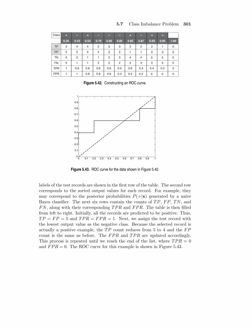
5.7 Class Imbalance Problem 301
0.25 0.43 0.53 0.76 0.85 0.85 0.85 0.87 0.93 0.95 1.00
Class + – + + + +– – – –
TP 5
5
0
0
1
1
4
5
0
1
0.8
1 2
1
4
4 3
0.8
0.8
1
4
0.6
2
2
3
3
0.6
2
2
3
3
0.6
2 3 3 4 5
5 54 4
1
3
1 0
2 2
0
1
5
0
0
0.6 0.4 0.4
0.2 0.2 0
0.2
0
0
00.40.60.81
TN
TPR
FPR
FN
FP
Figure 5.42. Constructing an ROC curve.
0.1
0.2
0.3
0.4
0.5
0.6
0.7
0.8
0.9
1
0 0
0.1
0.2
0.3
0.4
0.5
0.6
0.7
0.8
0.9
1
Figure 5.43. ROC curve for the data shown in Figure 5.42.
labels of the test records are shown in the first row of the table. The second rowcorresponds to the sorted output values for each record. For example, theymay correspond to the posterior probabilities P (+|x) generated by a naıveBayes classifier. The next six rows contain the counts of TP , FP , TN , andFN , along with their corresponding TPR and FPR. The table is then filledfrom left to right. Initially, all the records are predicted to be positive. Thus,TP = FP = 5 and TPR = FPR = 1. Next, we assign the test record withthe lowest output value as the negative class. Because the selected record isactually a positive example, the TP count reduces from 5 to 4 and the FPcount is the same as before. The FPR and TPR are updated accordingly.This process is repeated until we reach the end of the list, where TPR = 0and FPR = 0. The ROC curve for this example is shown in Figure 5.43.
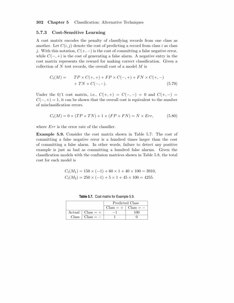
302 Chapter 5 Classification: Alternative Techniques
5.7.3 Cost-Sensitive Learning
A cost matrix encodes the penalty of classifying records from one class asanother. Let C(i, j) denote the cost of predicting a record from class i as classj. With this notation, C(+,−) is the cost of committing a false negative error,while C(−, +) is the cost of generating a false alarm. A negative entry in thecost matrix represents the reward for making correct classification. Given acollection of N test records, the overall cost of a model M is
Ct(M) = TP × C(+, +) + FP × C(−, +) + FN × C(+,−)
+ TN × C(−,−). (5.79)
Under the 0/1 cost matrix, i.e., C(+, +) = C(−,−) = 0 and C(+,−) =C(−, +) = 1, it can be shown that the overall cost is equivalent to the numberof misclassification errors.
Ct(M) = 0× (TP + TN) + 1× (FP + FN) = N × Err, (5.80)
where Err is the error rate of the classifier.
Example 5.9. Consider the cost matrix shown in Table 5.7: The cost ofcommitting a false negative error is a hundred times larger than the costof committing a false alarm. In other words, failure to detect any positiveexample is just as bad as committing a hundred false alarms. Given theclassification models with the confusion matrices shown in Table 5.8, the totalcost for each model is
Ct(M1) = 150× (−1) + 60× 1 + 40× 100 = 3910,
Ct(M2) = 250× (−1) + 5× 1 + 45× 100 = 4255.
Table 5.7. Cost matrix for Example 5.9.
Predicted ClassClass = + Class = −
Actual Class = + −1 100Class Class = − 1 0

5.7 Class Imbalance Problem 303
Table 5.8. Confusion matrix for two classification models.
Model M1 Predicted ClassClass + Class -
Actual Class + 150 40Class Class - 60 250
Model M2 Predicted ClassClass + Class -
Actual Class + 250 45Class Class - 5 200
Notice that despite improving both of its true positive and false positive counts,model M2 is still inferior since the improvement comes at the expense of in-creasing the more costly false negative errors. A standard accuracy measurewould have preferred model M2 over M1.
A cost-sensitive classification technique takes the cost matrix into consid-eration during model building and generates a model that has the lowest cost.For example, if false negative errors are the most costly, the learning algorithmwill try to reduce these errors by extending its decision boundary toward thenegative class, as shown in Figure 5.44. In this way, the generated model cancover more positive examples, although at the expense of generating additionalfalse alarms.
B2 B1
Figure 5.44. Modifying the decision boundary (from B1 to B2) to reduce the false negative errors of a
classifier.
There are various ways to incorporate cost information into classificationalgorithms. For example, in the context of decision tree induction, the cost

304 Chapter 5 Classification: Alternative Techniques
information can be used to: (1) choose the best attribute to use for splittingthe data, (2) determine whether a subtree should be pruned, (3) manipulatethe weights of the training records so that the learning algorithm converges toa decision tree that has the lowest cost, and (4) modify the decision rule ateach leaf node. To illustrate the last approach, let p(i|t) denote the fraction oftraining records from class i that belong to the leaf node t. A typical decisionrule for a binary classification problem assigns the positive class to node t ifthe following condition holds.
p(+|t) > p(−|t)=⇒ p(+|t) > (1− p(+|t))=⇒ 2p(+|t) > 1
=⇒ p(+|t) > 0.5. (5.81)
The preceding decision rule suggests that the class label of a leaf node dependson the majority class of the training records that reach the particular node.Note that this rule assumes that the misclassification costs are identical forboth positive and negative examples. This decision rule is equivalent to theexpression given in Equation 4.8 on page 165.
Instead of taking a majority vote, a cost-sensitive algorithm assigns theclass label i to node t if it minimizes the following expression:
C(i|t) =∑
j
p(j|t)C(j, i). (5.82)
In the case where C(+, +) = C(−,−) = 0, a leaf node t is assigned to thepositive class if:
p(+|t)C(+,−) > p(−|t)C(−, +)
=⇒ p(+|t)C(+,−) > (1− p(+|t))C(−, +)
=⇒ p(+|t) >C(−, +)
C(−, +) + C(+,−). (5.83)
This expression suggests that we can modify the threshold of the decision rulefrom 0.5 to C(−, +)/(C(−, +) + C(+,−)) to obtain a cost-sensitive classifier.If C(−, +) < C(+,−), then the threshold will be less than 0.5. This resultmakes sense because the cost of making a false negative error is more expensivethan that for generating a false alarm. Lowering the threshold will expand thedecision boundary toward the negative class, as shown in Figure 5.44.

5.7 Class Imbalance Problem 305
x1
x2
(a) Without oversampling
x1
x2
(b) With oversampling
Figure 5.45. Illustrating the effect of oversampling of the rare class.
5.7.4 Sampling-Based Approaches
Sampling is another widely used approach for handling the class imbalanceproblem. The idea of sampling is to modify the distribution of instances sothat the rare class is well represented in the training set. Some of the availabletechniques for sampling include undersampling, oversampling, and a hybridof both approaches. To illustrate these techniques, consider a data set thatcontains 100 positive examples and 1000 negative examples.
In the case of undersampling, a random sample of 100 negative examplesis chosen to form the training set along with all the positive examples. Onepotential problem with this approach is that some of the useful negative exam-ples may not be chosen for training, therefore, resulting in a less than optimalmodel. A potential method to overcome this problem is to perform undersam-pling multiple times and to induce multiple classifiers similar to the ensemblelearning approach. Focused undersampling methods may also be used, wherethe sampling procedure makes an informed choice with regard to the nega-tive examples that should be eliminated, e.g., those located far away from thedecision boundary.
Oversampling replicates the positive examples until the training set has anequal number of positive and negative examples. Figure 5.45 illustrates theeffect of oversampling on the construction of a decision boundary using a classi-fier such as a decision tree. Without oversampling, only the positive examplesat the bottom right-hand side of Figure 5.45(a) are classified correctly. Thepositive example in the middle of the diagram is misclassified because there

306 Chapter 5 Classification: Alternative Techniques
are not enough examples to justify the creation of a new decision boundaryto separate the positive and negative instances. Oversampling provides theadditional examples needed to ensure that the decision boundary surroundingthe positive example is not pruned, as illustrated in Figure 5.45(b).
However, for noisy data, oversampling may cause model overfitting becausesome of the noise examples may be replicated many times. In principle, over-sampling does not add any new information into the training set. Replicationof positive examples only prevents the learning algorithm from pruning certainparts of the model that describe regions that contain very few training exam-ples (i.e., the small disjuncts). The additional positive examples also tend toincrease the computation time for model building.
The hybrid approach uses a combination of undersampling the majorityclass and oversampling the rare class to achieve uniform class distribution.Undersampling can be performed using random or focused subsampling. Over-sampling, on the other hand, can be done by replicating the existing positiveexamples or generating new positive examples in the neighborhood of the ex-isting positive examples. In the latter approach, we must first determine thek-nearest neighbors for each existing positive example. A new positive ex-ample is then generated at some random point along the line segment thatjoins the positive example to one of its k-nearest neighbors. This process isrepeated until the desired number of positive examples is reached. Unlike thedata replication approach, the new examples allow us to extend the decisionboundary for the positive class outward, similar to the approach shown in Fig-ure 5.44. Nevertheless, this approach may still be quite susceptible to modeloverfitting.
5.8 Multiclass Problem
Some of the classification techniques described in this chapter, such as supportvector machines and AdaBoost, are originally designed for binary classificationproblems. Yet there are many real-world problems, such as character recogni-tion, face identification, and text classification, where the input data is dividedinto more than two categories. This section presents several approaches forextending the binary classifiers to handle multiclass problems. To illustratethese approaches, let Y = {y1, y2, . . . , yK} be the set of classes of the inputdata.
The first approach decomposes the multiclass problem into K binary prob-lems. For each class yi ∈ Y , a binary problem is created where all instancesthat belong to yi are considered positive examples, while the remaining in-

5.8 Multiclass Problem 307
stances are considered negative examples. A binary classifier is then con-structed to separate instances of class yi from the rest of the classes. This isknown as the one-against-rest (1-r) approach.
The second approach, which is known as the one-against-one (1-1) ap-proach, constructs K(K − 1)/2 binary classifiers, where each classifier is usedto distinguish between a pair of classes, (yi, yj). Instances that do not belongto either yi or yj are ignored when constructing the binary classifier for (yi, yj).In both 1-r and 1-1 approaches, a test instance is classified by combining thepredictions made by the binary classifiers. A voting scheme is typically em-ployed to combine the predictions, where the class that receives the highestnumber of votes is assigned to the test instance. In the 1-r approach, if aninstance is classified as negative, then all classes except for the positive classreceive a vote. This approach, however, may lead to ties among the differentclasses. Another possibility is to transform the outputs of the binary classifiersinto probability estimates and then assign the test instance to the class thathas the highest probability.
Example 5.10. Consider a multiclass problem where Y = {y1, y2, y3, y4}.Suppose a test instance is classified as (+,−,−,−) according to the 1-r ap-proach. In other words, it is classified as positive when y1 is used as thepositive class and negative when y2, y3, and y4 are used as the positive class.Using a simple majority vote, notice that y1 receives the highest number ofvotes, which is four, while the remaining classes receive only three votes. Thetest instance is therefore classified as y1.
Suppose the test instance is classified as follows using the 1-1 approach:
Binary pair +: y1 +: y1 +: y1 +: y2 +: y2 +: y3
of classes −: y2 −: y3 −: y4 −: y3 −: y4 −: y4
Classification + + − + − +
The first two rows in this table correspond to the pair of classes (yi, yj) chosento build the classifier and the last row represents the predicted class for the testinstance. After combining the predictions, y1 and y4 each receive two votes,while y2 and y3 each receives only one vote. The test instance is thereforeclassified as either y1 or y4, depending on the tie-breaking procedure.
Error-Correcting Output Coding
A potential problem with the previous two approaches is that they are sensitiveto the binary classification errors. For the 1-r approach given in Example 5.10,

308 Chapter 5 Classification: Alternative Techniques
if at least of one of the binary classifiers makes a mistake in its prediction, thenthe ensemble may end up declaring a tie between classes or making a wrongprediction. For example, suppose the test instance is classified as (+,−, +,−)due to misclassification by the third classifier. In this case, it will be difficult totell whether the instance should be classified as y1 or y3, unless the probabilityassociated with each class prediction is taken into account.
The error-correcting output coding (ECOC) method provides a more ro-bust way for handling multiclass problems. The method is inspired by aninformation-theoretic approach for sending messages across noisy channels.The idea behind this approach is to add redundancy into the transmittedmessage by means of a codeword, so that the receiver may detect errors in thereceived message and perhaps recover the original message if the number oferrors is small.
For multiclass learning, each class yi is represented by a unique bit string oflength n known as its codeword. We then train n binary classifiers to predicteach bit of the codeword string. The predicted class of a test instance is givenby the codeword whose Hamming distance is closest to the codeword producedby the binary classifiers. Recall that the Hamming distance between a pair ofbit strings is given by the number of bits that differ.
Example 5.11. Consider a multiclass problem where Y = {y1, y2, y3, y4}.Suppose we encode the classes using the following 7-bit codewords:
Class Codeword
y1 1 1 1 1 1 1 1y2 0 0 0 0 1 1 1y3 0 0 1 1 0 0 1y4 0 1 0 1 0 1 0
Each bit of the codeword is used to train a binary classifier. If a test instanceis classified as (0,1,1,1,1,1,1) by the binary classifiers, then the Hamming dis-tance between the codeword and y1 is 1, while the Hamming distance to theremaining classes is 3. The test instance is therefore classified as y1.
An interesting property of an error-correcting code is that if the minimumHamming distance between any pair of codewords is d, then any ⌊(d− 1)/2)⌋errors in the output code can be corrected using its nearest codeword. InExample 5.11, because the minimum Hamming distance between any pair ofcodewords is 4, the ensemble may tolerate errors made by one of the seven

5.9 Bibliographic Notes 309
binary classifiers. If there is more than one classifier that makes a mistake,then the ensemble may not be able to compensate for the error.
An important issue is how to design the appropriate set of codewords fordifferent classes. From coding theory, a vast number of algorithms have beendeveloped for generating n-bit codewords with bounded Hamming distance.However, the discussion of these algorithms is beyond the scope of this book.It is worthwhile mentioning that there is a significant difference between thedesign of error-correcting codes for communication tasks compared to thoseused for multiclass learning. For communication, the codewords should max-imize the Hamming distance between the rows so that error correction canbe performed. Multiclass learning, however, requires that the row-wise andcolumn-wise distances of the codewords must be well separated. A largercolumn-wise distance ensures that the binary classifiers are mutually indepen-dent, which is an important requirement for ensemble learning methods.
5.9 Bibliographic Notes
Mitchell [208] provides an excellent coverage on many classification techniquesfrom a machine learning perspective. Extensive coverage on classification canalso be found in Duda et al. [180], Webb [219], Fukunaga [187], Bishop [159],Hastie et al. [192], Cherkassky and Mulier [167], Witten and Frank [221], Handet al. [190], Han and Kamber [189], and Dunham [181].
Direct methods for rule-based classifiers typically employ the sequentialcovering scheme for inducing classification rules. Holte’s 1R [195] is the sim-plest form of a rule-based classifier because its rule set contains only a singlerule. Despite its simplicity, Holte found that for some data sets that exhibita strong one-to-one relationship between the attributes and the class label,1R performs just as well as other classifiers. Other examples of rule-basedclassifiers include IREP [184], RIPPER [170], CN2 [168, 169], AQ [207], RISE[176], and ITRULE [214]. Table 5.9 shows a comparison of the characteristicsof four of these classifiers.
For rule-based classifiers, the rule antecedent can be generalized to includeany propositional or first-order logical expression (e.g., Horn clauses). Read-ers who are interested in first-order logic rule-based classifiers may refer toreferences such as [208] or the vast literature on inductive logic programming[209]. Quinlan [211] proposed the C4.5rules algorithm for extracting classifi-cation rules from decision trees. An indirect method for extracting rules fromartificial neural networks was given by Andrews et al. in [157].

310 Chapter 5 Classification: Alternative Techniques
Table 5.9. Comparison of various rule-based classifiers.
RIPPER CN2 CN2 AQR(unordered) (ordered)
Rule-growing General-to- General-to- General-to- General-to-specificstrategy specific specific specific (seeded by a
positive example)Evaluation FOIL’s Info gain Laplace Entropy and Number ofMetric likelihood ratio true positivesStopping All examples No performance No performance Rules cover onlycondition for belong to the gain gain positive classrule-growing same classRule Pruning Reduced None None None
error pruningInstance Positive and Positive only Positive only Positive andElimination negative negativeStopping Error > 50% or No performance No performance All positivecondition for based on MDL gain gain examples areadding rules coveredRule Set Replace or Statistical None NonePruning modify rules testsSearch strategy Greedy Beam search Beam search Beam search
Cover and Hart [172] presented an overview of the nearest-neighbor classi-fication method from a Bayesian perspective. Aha provided both theoreticaland empirical evaluations for instance-based methods in [155]. PEBLS, whichwas developed by Cost and Salzberg [171], is a nearest-neighbor classificationalgorithm that can handle data sets containing nominal attributes. Each train-ing example in PEBLS is also assigned a weight factor that depends on thenumber of times the example helps make a correct prediction. Han et al. [188]developed a weight-adjusted nearest-neighbor algorithm, in which the featureweights are learned using a greedy, hill-climbing optimization algorithm.
Naıve Bayes classifiers have been investigated by many authors, includingLangley et al. [203], Ramoni and Sebastiani [212], Lewis [204], and Domingosand Pazzani [178]. Although the independence assumption used in naıve Bayesclassifiers may seem rather unrealistic, the method has worked surprisingly wellfor applications such as text classification. Bayesian belief networks provide amore flexible approach by allowing some of the attributes to be interdependent.An excellent tutorial on Bayesian belief networks is given by Heckerman in[194].
Vapnik [217, 218] had written two authoritative books on Support VectorMachines (SVM). Other useful resources on SVM and kernel methods includethe books by Cristianini and Shawe-Taylor [173] and Scholkopf and Smola

5.9 Bibliographic Notes 311
[213]. There are several survey articles on SVM, including those written byBurges [164], Bennet et al. [158], Hearst [193], and Mangasarian [205].
A survey of ensemble methods in machine learning was given by Diet-terich [174]. The bagging method was proposed by Breiman [161]. Freundand Schapire [186] developed the AdaBoost algorithm. Arcing, which standsfor adaptive resampling and combining, is a variant of the boosting algorithmproposed by Breiman [162]. It uses the non-uniform weights assigned to train-ing examples to resample the data for building an ensemble of training sets.Unlike AdaBoost, the votes of the base classifiers are not weighted when de-termining the class label of test examples. The random forest method wasintroduced by Breiman in [163].
Related work on mining rare and imbalanced data sets can be found in thesurvey papers written by Chawla et al. [166] and Weiss [220]. Sampling-basedmethods for mining imbalanced data sets have been investigated by many au-thors, such as Kubat and Matwin [202], Japkowitz [196], and Drummond andHolte [179]. Joshi et al. [199] discussed the limitations of boosting algorithmsfor rare class modeling. Other algorithms developed for mining rare classesinclude SMOTE [165], PNrule [198], and CREDOS [200].
Various alternative metrics that are well-suited for class imbalanced prob-lems are available. The precision, recall, and F1-measure are widely used met-rics in information retrieval [216]. ROC analysis was originally used in signaldetection theory. Bradley [160] investigated the use of area under the ROCcurve as a performance metric for machine learning algorithms. A methodfor comparing classifier performance using the convex hull of ROC curves wassuggested by Provost and Fawcett in [210]. Ferri et al. [185] developed amethodology for performing ROC analysis on decision tree classifiers. Theyhad also proposed a methodology for incorporating area under the ROC curve(AUC) as the splitting criterion during the tree-growing process. Joshi [197]examined the performance of these measures from the perspective of analyzingrare classes.
A vast amount of literature on cost-sensitive learning can be found inthe online proceedings of the ICML’2000 Workshop on cost-sensitive learn-ing. The properties of a cost matrix had been studied by Elkan in [182].Margineantu and Dietterich [206] examined various methods for incorporatingcost information into the C4.5 learning algorithm, including wrapper meth-ods, class distribution-based methods, and loss-based methods. Other cost-sensitive learning methods that are algorithm-independent include AdaCost[183], MetaCost [177], and costing [222].

312 Chapter 5 Classification: Alternative Techniques
Extensive literature is also available on the subject of multiclass learning.This includes the works of Hastie and Tibshirani [191], Allwein et al. [156],Kong and Dietterich [201], and Tax and Duin [215]. The error-correctingoutput coding (ECOC) method was proposed by Dietterich and Bakiri [175].They had also investigated techniques for designing codes that are suitable forsolving multiclass problems.
Bibliography[155] D. W. Aha. A study of instance-based algorithms for supervised learning tasks: mathe-
matical, empirical, and psychological evaluations. PhD thesis, University of California,Irvine, 1990.
[156] E. L. Allwein, R. E. Schapire, and Y. Singer. Reducing Multiclass to Binary: AUnifying Approach to Margin Classifiers. Journal of Machine Learning Research, 1:113–141, 2000.
[157] R. Andrews, J. Diederich, and A. Tickle. A Survey and Critique of Techniques ForExtracting Rules From Trained Artificial Neural Networks. Knowledge Based Systems,8(6):373–389, 1995.
[158] K. Bennett and C. Campbell. Support Vector Machines: Hype or Hallelujah. SIGKDDExplorations, 2(2):1–13, 2000.
[159] C. M. Bishop. Neural Networks for Pattern Recognition. Oxford University Press,Oxford, U.K., 1995.
[160] A. P. Bradley. The use of the area under the ROC curve in the Evaluation of MachineLearning Algorithms. Pattern Recognition, 30(7):1145–1149, 1997.
[161] L. Breiman. Bagging Predictors. Machine Learning, 24(2):123–140, 1996.
[162] L. Breiman. Bias, Variance, and Arcing Classifiers. Technical Report 486, Universityof California, Berkeley, CA, 1996.
[163] L. Breiman. Random Forests. Machine Learning, 45(1):5–32, 2001.
[164] C. J. C. Burges. A Tutorial on Support Vector Machines for Pattern Recognition.Data Mining and Knowledge Discovery, 2(2):121–167, 1998.
[165] N. V. Chawla, K. W. Bowyer, L. O. Hall, and W. P. Kegelmeyer. SMOTE: SyntheticMinority Over-sampling Technique. Journal of Artificial Intelligence Research, 16:321–357, 2002.
[166] N. V. Chawla, N. Japkowicz, and A. Kolcz. Editorial: Special Issue on Learning fromImbalanced Data Sets. SIGKDD Explorations, 6(1):1–6, 2004.
[167] V. Cherkassky and F. Mulier. Learning from Data: Concepts, Theory, and Methods.Wiley Interscience, 1998.
[168] P. Clark and R. Boswell. Rule Induction with CN2: Some Recent Improvements. InMachine Learning: Proc. of the 5th European Conf. (EWSL-91), pages 151–163, 1991.
[169] P. Clark and T. Niblett. The CN2 Induction Algorithm. Machine Learning, 3(4):261–283, 1989.
[170] W. W. Cohen. Fast Effective Rule Induction. In Proc. of the 12th Intl. Conf. onMachine Learning, pages 115–123, Tahoe City, CA, July 1995.
[171] S. Cost and S. Salzberg. A Weighted Nearest Neighbor Algorithm for Learning withSymbolic Features. Machine Learning, 10:57–78, 1993.
[172] T. M. Cover and P. E. Hart. Nearest Neighbor Pattern Classification. KnowledgeBased Systems, 8(6):373–389, 1995.

Bibliography 313
[173] N. Cristianini and J. Shawe-Taylor. An Introduction to Support Vector Machines andOther Kernel-based Learning Methods. Cambridge University Press, 2000.
[174] T. G. Dietterich. Ensemble Methods in Machine Learning. In First Intl. Workshop onMultiple Classifier Systems, Cagliari, Italy, 2000.
[175] T. G. Dietterich and G. Bakiri. Solving Multiclass Learning Problems via Error-Correcting Output Codes. Journal of Artificial Intelligence Research, 2:263–286, 1995.
[176] P. Domingos. The RISE system: Conquering without separating. In Proc. of the 6thIEEE Intl. Conf. on Tools with Artificial Intelligence, pages 704–707, New Orleans, LA,1994.
[177] P. Domingos. MetaCost: A General Method for Making Classifiers Cost-Sensitive. InProc. of the 5th Intl. Conf. on Knowledge Discovery and Data Mining, pages 155–164,San Diego, CA, August 1999.
[178] P. Domingos and M. Pazzani. On the Optimality of the Simple Bayesian Classifierunder Zero-One Loss. Machine Learning, 29(2-3):103–130, 1997.
[179] C. Drummond and R. C. Holte. C4.5, Class imbalance, and Cost sensitivity: Whyunder-sampling beats over-sampling. In ICML’2004 Workshop on Learning from Im-balanced Data Sets II, Washington, DC, August 2003.
[180] R. O. Duda, P. E. Hart, and D. G. Stork. Pattern Classification. John Wiley & Sons,Inc., New York, 2nd edition, 2001.
[181] M. H. Dunham. Data Mining: Introductory and Advanced Topics. Prentice Hall, 2002.
[182] C. Elkan. The Foundations of Cost-Sensitive Learning. In Proc. of the 17th Intl. JointConf. on Artificial Intelligence, pages 973–978, Seattle, WA, August 2001.
[183] W. Fan, S. J. Stolfo, J. Zhang, and P. K. Chan. AdaCost: misclassification cost-sensitive boosting. In Proc. of the 16th Intl. Conf. on Machine Learning, pages 97–105,Bled, Slovenia, June 1999.
[184] J. Furnkranz and G. Widmer. Incremental reduced error pruning. In Proc. of the 11thIntl. Conf. on Machine Learning, pages 70–77, New Brunswick, NJ, July 1994.
[185] C. Ferri, P. Flach, and J. Hernandez-Orallo. Learning Decision Trees Using the AreaUnder the ROC Curve. In Proc. of the 19th Intl. Conf. on Machine Learning, pages139–146, Sydney, Australia, July 2002.
[186] Y. Freund and R. E. Schapire. A decision-theoretic generalization of on-line learningand an application to boosting. Journal of Computer and System Sciences, 55(1):119–139, 1997.
[187] K. Fukunaga. Introduction to Statistical Pattern Recognition. Academic Press, NewYork, 1990.
[188] E.-H. Han, G. Karypis, and V. Kumar. Text Categorization Using Weight Adjustedk-Nearest Neighbor Classification. In Proc. of the 5th Pacific-Asia Conf. on KnowledgeDiscovery and Data Mining, Lyon, France, 2001.
[189] J. Han and M. Kamber. Data Mining: Concepts and Techniques. Morgan KaufmannPublishers, San Francisco, 2001.
[190] D. J. Hand, H. Mannila, and P. Smyth. Principles of Data Mining. MIT Press, 2001.
[191] T. Hastie and R. Tibshirani. Classification by pairwise coupling. Annals of Statistics,26(2):451–471, 1998.
[192] T. Hastie, R. Tibshirani, and J. H. Friedman. The Elements of Statistical Learning:Data Mining, Inference, Prediction. Springer, New York, 2001.
[193] M. Hearst. Trends & Controversies: Support Vector Machines. IEEE IntelligentSystems, 13(4):18–28, 1998.

314 Chapter 5 Classification: Alternative Techniques
[194] D. Heckerman. Bayesian Networks for Data Mining. Data Mining and KnowledgeDiscovery, 1(1):79–119, 1997.
[195] R. C. Holte. Very Simple Classification Rules Perform Well on Most Commonly UsedData sets. Machine Learning, 11:63–91, 1993.
[196] N. Japkowicz. The Class Imbalance Problem: Significance and Strategies. In Proc.of the 2000 Intl. Conf. on Artificial Intelligence: Special Track on Inductive Learning,volume 1, pages 111–117, Las Vegas, NV, June 2000.
[197] M. V. Joshi. On Evaluating Performance of Classifiers for Rare Classes. In Proc. ofthe 2002 IEEE Intl. Conf. on Data Mining, Maebashi City, Japan, December 2002.
[198] M. V. Joshi, R. C. Agarwal, and V. Kumar. Mining Needles in a Haystack: ClassifyingRare Classes via Two-Phase Rule Induction. In Proc. of 2001 ACM-SIGMOD Intl. Conf.on Management of Data, pages 91–102, Santa Barbara, CA, June 2001.
[199] M. V. Joshi, R. C. Agarwal, and V. Kumar. Predicting rare classes: can boostingmake any weak learner strong? In Proc. of the 8th Intl. Conf. on Knowledge Discoveryand Data Mining, pages 297–306, Edmonton, Canada, July 2002.
[200] M. V. Joshi and V. Kumar. CREDOS: Classification Using Ripple Down Structure(A Case for Rare Classes). In Proc. of the SIAM Intl. Conf. on Data Mining, pages321–332, Orlando, FL, April 2004.
[201] E. B. Kong and T. G. Dietterich. Error-Correcting Output Coding Corrects Bias andVariance. In Proc. of the 12th Intl. Conf. on Machine Learning, pages 313–321, TahoeCity, CA, July 1995.
[202] M. Kubat and S. Matwin. Addressing the Curse of Imbalanced Training Sets: OneSided Selection. In Proc. of the 14th Intl. Conf. on Machine Learning, pages 179–186,Nashville, TN, July 1997.
[203] P. Langley, W. Iba, and K. Thompson. An analysis of Bayesian classifiers. In Proc. ofthe 10th National Conf. on Artificial Intelligence, pages 223–228, 1992.
[204] D. D. Lewis. Naive Bayes at Forty: The Independence Assumption in InformationRetrieval. In Proc. of the 10th European Conf. on Machine Learning (ECML 1998),pages 4–15, 1998.
[205] O. Mangasarian. Data Mining via Support Vector Machines. Technical Report Tech-nical Report 01-05, Data Mining Institute, May 2001.
[206] D. D. Margineantu and T. G. Dietterich. Learning Decision Trees for Loss Minimizationin Multi-Class Problems. Technical Report 99-30-03, Oregon State University, 1999.
[207] R. S. Michalski, I. Mozetic, J. Hong, and N. Lavrac. The Multi-Purpose IncrementalLearning System AQ15 and Its Testing Application to Three Medical Domains. In Proc.of 5th National Conf. on Artificial Intelligence, Orlando, August 1986.
[208] T. Mitchell. Machine Learning. McGraw-Hill, Boston, MA, 1997.
[209] S. Muggleton. Foundations of Inductive Logic Programming. Prentice Hall, EnglewoodCliffs, NJ, 1995.
[210] F. J. Provost and T. Fawcett. Analysis and Visualization of Classifier Performance:Comparison under Imprecise Class and Cost Distributions. In Proc. of the 3rd Intl.Conf. on Knowledge Discovery and Data Mining, pages 43–48, Newport Beach, CA,August 1997.
[211] J. R. Quinlan. C4.5: Programs for Machine Learning. Morgan-Kaufmann Publishers,San Mateo, CA, 1993.
[212] M. Ramoni and P. Sebastiani. Robust Bayes classifiers. Artificial Intelligence, 125:209–226, 2001.

5.10 Exercises 315
[213] B. Scholkopf and A. J. Smola. Learning with Kernels: Support Vector Machines,Regularization, Optimization, and Beyond. MIT Press, 2001.
[214] P. Smyth and R. M. Goodman. An Information Theoretic Approach to Rule Inductionfrom Databases. IEEE Trans. on Knowledge and Data Engineering, 4(4):301–316, 1992.
[215] D. M. J. Tax and R. P. W. Duin. Using Two-Class Classifiers for Multiclass Classi-fication. In Proc. of the 16th Intl. Conf. on Pattern Recognition (ICPR 2002), pages124–127, Quebec, Canada, August 2002.
[216] C. J. van Rijsbergen. Information Retrieval. Butterworth-Heinemann, Newton, MA,1978.
[217] V. Vapnik. The Nature of Statistical Learning Theory. Springer Verlag, New York,1995.
[218] V. Vapnik. Statistical Learning Theory. John Wiley & Sons, New York, 1998.
[219] A. R. Webb. Statistical Pattern Recognition. John Wiley & Sons, 2nd edition, 2002.
[220] G. M. Weiss. Mining with Rarity: A Unifying Framework. SIGKDD Explorations, 6(1):7–19, 2004.
[221] I. H. Witten and E. Frank. Data Mining: Practical Machine Learning Tools andTechniques with Java Implementations. Morgan Kaufmann, 1999.
[222] B. Zadrozny, J. C. Langford, and N. Abe. Cost-Sensitive Learning by Cost-Proportionate Example Weighting. In Proc. of the 2003 IEEE Intl. Conf. on DataMining, pages 435–442, Melbourne, FL, August 2003.
5.10 Exercises
1. Consider a binary classification problem with the following set of attributes andattribute values:
• Air Conditioner = {Working, Broken}• Engine = {Good, Bad}• Mileage = {High, Medium, Low}• Rust = {Yes, No}
Suppose a rule-based classifier produces the following rule set:
Mileage = High −→ Value = LowMileage = Low −→ Value = HighAir Conditioner = Working, Engine = Good −→ Value = HighAir Conditioner = Working, Engine = Bad −→ Value = LowAir Conditioner = Broken −→ Value = Low
(a) Are the rules mutually exclustive?

316 Chapter 5 Classification: Alternative Techniques
(b) Is the rule set exhaustive?
(c) Is ordering needed for this set of rules?
(d) Do you need a default class for the rule set?
2. The RIPPER algorithm (by Cohen [170]) is an extension of an earlier algorithmcalled IREP (by Furnkranz and Widmer [184]). Both algorithms apply thereduced-error pruning method to determine whether a rule needs to bepruned. The reduced error pruning method uses a validation set to estimatethe generalization error of a classifier. Consider the following pair of rules:
R1: A −→ CR2: A ∧B −→ C
R2 is obtained by adding a new conjunct, B, to the left-hand side of R1. Forthis question, you will be asked to determine whether R2 is preferred over R1
from the perspectives of rule-growing and rule-pruning. To determine whethera rule should be pruned, IREP computes the following measure:
vIREP =p + (N − n)
P + N,
where P is the total number of positive examples in the validation set, N isthe total number of negative examples in the validation set, p is the number ofpositive examples in the validation set covered by the rule, and n is the numberof negative examples in the validation set covered by the rule. vIREP is actuallysimilar to classification accuracy for the validation set. IREP favors rules thathave higher values of vIREP . On the other hand, RIPPER applies the followingmeasure to determine whether a rule should be pruned:
vRIPPER =p− n
p + n.
(a) Suppose R1 is covered by 350 positive examples and 150 negative ex-amples, while R2 is covered by 300 positive examples and 50 negativeexamples. Compute the FOIL’s information gain for the rule R2 withrespect to R1.
(b) Consider a validation set that contains 500 positive examples and 500negative examples. For R1, suppose the number of positive examplescovered by the rule is 200, and the number of negative examples coveredby the rule is 50. For R2, suppose the number of positive examples coveredby the rule is 100 and the number of negative examples is 5. ComputevIREP for both rules. Which rule does IREP prefer?
(c) Compute vRIPPER for the previous problem. Which rule does RIPPERprefer?

5.10 Exercises 317
3. C4.5rules is an implementation of an indirect method for generating rules froma decision tree. RIPPER is an implementation of a direct method for generatingrules directly from data.
(a) Discuss the strengths and weaknesses of both methods.
(b) Consider a data set that has a large difference in the class size (i.e., someclasses are much bigger than others). Which method (between C4.5rulesand RIPPER) is better in terms of finding high accuracy rules for thesmall classes?
4. Consider a training set that contains 100 positive examples and 400 negativeexamples. For each of the following candidate rules,
R1: A −→ + (covers 4 positive and 1 negative examples),R2: B −→ + (covers 30 positive and 10 negative examples),R3: C −→ + (covers 100 positive and 90 negative examples),
determine which is the best and worst candidate rule according to:
(a) Rule accuracy.
(b) FOIL’s information gain.
(c) The likelihood ratio statistic.
(d) The Laplace measure.
(e) The m-estimate measure (with k = 2 and p+ = 0.2).
5. Figure 5.4 illustrates the coverage of the classification rules R1, R2, and R3.Determine which is the best and worst rule according to:
(a) The likelihood ratio statistic.
(b) The Laplace measure.
(c) The m-estimate measure (with k = 2 and p+ = 0.58).
(d) The rule accuracy after R1 has been discovered, where none of the exam-ples covered by R1 are discarded).
(e) The rule accuracy after R1 has been discovered, where only the positiveexamples covered by R1 are discarded).
(f) The rule accuracy after R1 has been discovered, where both positive andnegative examples covered by R1 are discarded.
6. (a) Suppose the fraction of undergraduate students who smoke is 15% andthe fraction of graduate students who smoke is 23%. If one-fifth of thecollege students are graduate students and the rest are undergraduates,what is the probability that a student who smokes is a graduate student?

318 Chapter 5 Classification: Alternative Techniques
(b) Given the information in part (a), is a randomly chosen college studentmore likely to be a graduate or undergraduate student?
(c) Repeat part (b) assuming that the student is a smoker.
(d) Suppose 30% of the graduate students live in a dorm but only 10% ofthe undergraduate students live in a dorm. If a student smokes and livesin the dorm, is he or she more likely to be a graduate or undergraduatestudent? You can assume independence between students who live in adorm and those who smoke.
7. Consider the data set shown in Table 5.10
Table 5.10. Data set for Exercise 7.
Record A B C Class
1 0 0 0 +2 0 0 1 −3 0 1 1 −4 0 1 1 −5 0 0 1 +6 1 0 1 +7 1 0 1 −8 1 0 1 −9 1 1 1 +10 1 0 1 +
(a) Estimate the conditional probabilities for P (A|+), P (B|+), P (C|+), P (A|−),P (B|−), and P (C|−).
(b) Use the estimate of conditional probabilities given in the previous questionto predict the class label for a test sample (A = 0, B = 1, C = 0) usingthe naıve Bayes approach.
(c) Estimate the conditional probabilities using the m-estimate approach,with p = 1/2 and m = 4.
(d) Repeat part (b) using the conditional probabilities given in part (c).
(e) Compare the two methods for estimating probabilities. Which method isbetter and why?
8. Consider the data set shown in Table 5.11.
(a) Estimate the conditional probabilities for P (A = 1|+), P (B = 1|+),P (C = 1|+), P (A = 1|−), P (B = 1|−), and P (C = 1|−) using thesame approach as in the previous problem.

5.10 Exercises 319
Table 5.11. Data set for Exercise 8.
Instance A B C Class
1 0 0 1 −2 1 0 1 +3 0 1 0 −4 1 0 0 −5 1 0 1 +6 0 0 1 +7 1 1 0 −8 0 0 0 −9 0 1 0 +10 1 1 1 +
(b) Use the conditional probabilities in part (a) to predict the class label fora test sample (A = 1, B = 1, C = 1) using the naıve Bayes approach.
(c) Compare P (A = 1), P (B = 1), and P (A = 1, B = 1). State the relation-ships between A and B.
(d) Repeat the analysis in part (c) using P (A = 1), P (B = 0), and P (A =1, B = 0).
(e) Compare P (A = 1, B = 1|Class = +) against P (A = 1|Class = +) andP (B = 1|Class = +). Are the variables conditionally independent giventhe class?
9. (a) Explain how naıve Bayes performs on the data set shown in Figure 5.46.
(b) If each class is further divided such that there are four classes (A1, A2,B1, and B2), will naıve Bayes perform better?
(c) How will a decision tree perform on this data set (for the two-class prob-lem)? What if there are four classes?
10. Repeat the analysis shown in Example 5.3 for finding the location of a decisionboundary using the following information:
(a) The prior probabilities are P (Crocodile) = 2× P (Alligator).
(b) The prior probabilities are P (Alligator) = 2× P (Crocodile).
(c) The prior probabilities are the same, but their standard deviations aredifferent; i.e., σ(Crocodile) = 4 and σ(Alligator) = 2.
11. Figure 5.47 illustrates the Bayesian belief network for the data set shown inTable 5.12. (Assume that all the attributes are binary).
(a) Draw the probability table for each node in the network.

320 Chapter 5 Classification: Alternative Techniques
Distinguishing Attributes Noise Attributes
Class A
Class B
Records
Attributes
A1
A2
B1
B2
Figure 5.46. Data set for Exercise 9.
Mileage
Engine
Car Value
Air Conditioner
Figure 5.47. Bayesian belief network.
(b) Use the Bayesian network to compute P(Engine = Bad, Air Conditioner= Broken).
12. Given the Bayesian network shown in Figure 5.48, compute the following prob-abilities:
(a) P (B = good, F = empty, G = empty, S = yes).
(b) P (B = bad, F = empty, G = not empty, S = no).
(c) Given that the battery is bad, compute the probability that the car willstart.
13. Consider the one-dimensional data set shown in Table 5.13.

5.10 Exercises 321
Table 5.12. Data set for Exercise 11.
Mileage Engine Air Conditioner Number of Records Number of Recordswith Car Value=Hi with Car Value=Lo
Hi Good Working 3 4Hi Good Broken 1 2Hi Bad Working 1 5Hi Bad Broken 0 4Lo Good Working 9 0Lo Good Broken 5 1Lo Bad Working 1 2Lo Bad Broken 0 2
Battery
Gauge
Start
Fuel
P(B = bad) = 0.1 P(F = empty) = 0.2
P(G = empty | B = good, F = not empty) = 0.1 P(G = empty | B = good, F = empty) = 0.8 P(G = empty | B = bad, F = not empty) = 0.2 P(G = empty | B = bad, F = empty) = 0.9
P(S = no | B = good, F = not empty) = 0.1 P(S = no | B = good, F = empty) = 0.8 P(S = no | B = bad, F = not empty) = 0.9 P(S = no | B = bad, F = empty) = 1.0
Figure 5.48. Bayesian belief network for Exercise 12.
(a) Classify the data point x = 5.0 according to its 1-, 3-, 5-, and 9-nearestneighbors (using majority vote).
(b) Repeat the previous analysis using the distance-weighted voting approachdescribed in Section 5.2.1.
14. The nearest-neighbor algorithm described in Section 5.2 can be extended tohandle nominal attributes. A variant of the algorithm called PEBLS (ParallelExamplar-Based Learning System) by Cost and Salzberg [171] measures thedistance between two values of a nominal attribute using the modified valuedifference metric (MVDM). Given a pair of nominal attribute values, V1 and

322 Chapter 5 Classification: Alternative Techniques
Table 5.13. Data set for Exercise 13.
x 0.5 3.0 4.5 4.6 4.9 5.2 5.3 5.5 7.0 9.5y − − + + + − − + − −
V2, the distance between them is defined as follows:
d(V1, V2) =
k∑
i=1
∣∣∣∣ni1
n1− ni2
n2
∣∣∣∣, (5.84)
where nij is the number of examples from class i with attribute value Vj andnj is the number of examples with attribute value Vj .
Consider the training set for the loan classification problem shown in Figure5.9. Use the MVDM measure to compute the distance between every pair ofattribute values for the Home Owner and Marital Status attributes.
15. For each of the Boolean functions given below, state whether the problem islinearly separable.
(a) A AND B AND C
(b) NOT A AND B
(c) (A OR B) AND (A OR C)
(d) (A XOR B) AND (A OR B)
16. (a) Demonstrate how the perceptron model can be used to represent the ANDand OR functions between a pair of Boolean variables.
(b) Comment on the disadvantage of using linear functions as activation func-tions for multilayer neural networks.
17. You are asked to evaluate the performance of two classification models, M1 andM2. The test set you have chosen contains 26 binary attributes, labeled as Athrough Z.
Table 5.14 shows the posterior probabilities obtained by applying the modelsto the test set. (Only the posterior probabilities for the positive class areshown). As this is a two-class problem, P (−) = 1−P (+) and P (−|A, . . . , Z) =1−P (+|A, . . . , Z). Assume that we are mostly interested in detecting instancesfrom the positive class.
(a) Plot the ROC curve for both M1 and M2. (You should plot them on thesame graph.) Which model do you think is better? Explain your reasons.
(b) For model M1, suppose you choose the cutoff threshold to be t = 0.5. Inother words, any test instances whose posterior probability is greater thant will be classified as a positive example. Compute the precision, recall,and F-measure for the model at this threshold value.

5.10 Exercises 323
Table 5.14. Posterior probabilities for Exercise 17.
Instance True Class P (+|A, . . . , Z,M1) P (+|A, . . . , Z,M2)1 + 0.73 0.612 + 0.69 0.033 − 0.44 0.684 − 0.55 0.315 + 0.67 0.456 + 0.47 0.097 − 0.08 0.388 − 0.15 0.059 + 0.45 0.0110 − 0.35 0.04
(c) Repeat the analysis for part (c) using the same cutoff threshold on modelM2. Compare the F -measure results for both models. Which model isbetter? Are the results consistent with what you expect from the ROCcurve?
(d) Repeat part (c) for model M1 using the threshold t = 0.1. Which thresh-old do you prefer, t = 0.5 or t = 0.1? Are the results consistent with whatyou expect from the ROC curve?
18. Following is a data set that contains two attributes, X and Y , and two classlabels, “+” and “−”. Each attribute can take three different values: 0, 1, or 2.
X YNumber ofInstances+ −
0 0 0 1001 0 0 02 0 0 1000 1 10 1001 1 10 02 1 10 1000 2 0 1001 2 0 02 2 0 100
The concept for the “+” class is Y = 1 and the concept for the “−” class isX = 0 ∨X = 2.
(a) Build a decision tree on the data set. Does the tree capture the “+” and“−” concepts?

324 Chapter 5 Classification: Alternative Techniques
(b) What are the accuracy, precision, recall, and F1-measure of the decisiontree? (Note that precision, recall, and F1-measure are defined with respectto the “+” class.)
(c) Build a new decision tree with the following cost function:
C(i, j) =
0, if i = j;1, if i = +, j = −;Number of − instancesNumber of + instances , if i = −, j = +.
(Hint: only the leaves of the old decision tree need to be changed.) Doesthe decision tree capture the “+” concept?
(d) What are the accuracy, precision, recall, and F1-measure of the new deci-sion tree?
19. (a) Consider the cost matrix for a two-class problem. Let C(+,+) = C(−,−) =p, C(+,−) = C(−,+) = q, and q > p. Show that minimizing the costfunction is equivalent to maximizing the classifier’s accuracy.
(b) Show that a cost matrix is scale-invariant. For example, if the cost matrixis rescaled from C(i, j) −→ βC(i, j), where β is the scaling factor, thedecision threshold (Equation 5.82) will remain unchanged.
(c) Show that a cost matrix is translation-invariant. In other words, adding aconstant factor to all entries in the cost matrix will not affect the decisionthreshold (Equation 5.82).
20. Consider the task of building a classifier from random data, where the attributevalues are generated randomly irrespective of the class labels. Assume the dataset contains records from two classes, “+” and “−.” Half of the data set is usedfor training while the remaining half is used for testing.
(a) Suppose there are an equal number of positive and negative records inthe data and the decision tree classifier predicts every test record to bepositive. What is the expected error rate of the classifier on the test data?
(b) Repeat the previous analysis assuming that the classifier predicts eachtest record to be positive class with probability 0.8 and negative classwith probability 0.2.
(c) Suppose two-thirds of the data belong to the positive class and the re-maining one-third belong to the negative class. What is the expectederror of a classifier that predicts every test record to be positive?
(d) Repeat the previous analysis assuming that the classifier predicts eachtest record to be positive class with probability 2/3 and negative classwith probability 1/3.

5.10 Exercises 325
21. Derive the dual Lagrangian for the linear SVM with nonseparable data wherethe objective function is
f(w) =‖w‖2
2+ C
( N∑
i=1
ξi
)2.
22. Consider the XOR problem where there are four training points:
(1, 1,−), (1, 0,+), (0, 1,+), (0, 0,−).
Transform the data into the following feature space:
Φ = (1,√
2x1,√
2x2,√
2x1x2, x21, x
22).
Find the maximum margin linear decision boundary in the transformed space.
23. Given the data sets shown in Figures 5.49, explain how the decision tree, naıveBayes, and k-nearest neighbor classifiers would perform on these data sets.

326 Chapter 5 Classification: Alternative Techniques
Distinguishing Attributes Noise Attributes
Class A
Class B
Records
Attributes
(a) Synthetic data set 1.
Distinguishing Attributes Noise Attributes
Class A
Class B
Records
Attributes
(b) Synthetic data set 2.
Distinguishing Attribute set 1 Noise Attributes
Class A
Class B
Records
Attributes
Distinguishing Attribute set 2
60% filled with 1
60% filled with 1
40% filled with 1
40% filled with 1
(c) Synthetic data set 3.
Class A Class B Class A Class B Class A
Class A Class B Class A Class BClass B
Class A Class B Class A Class B Class A
Class A Class B Class A Class BClass B
Attribute X
Att
rib
ute
Y
(d) Synthetic data set 4
Attribute X
Att
rib
ute
Y
Class A
Class B
(e) Synthetic data set 5.
Attribute X
Att
rib
ute
Y
Class A
Class B
Class B
(f) Synthetic data set 6.
Figure 5.49. Data set for Exercise 23.