classification of images based on pixels that …
TRANSCRIPT
Kennesaw State UniversityDigitalCommons@Kennesaw State University
Master of Science in Computer Science Theses Department of Computer Science
Spring 5-9-2017
CLASSIFICATION OF IMAGES BASED ONPIXELS THAT REPRESENT A SMALL PARTOF THE SCENE. A CASE APPLIED TOMICROANEURYSMS IN FUNDUS RETINAIMAGESPablo F. OrdonezKennesaw State University
Pablo F. Ordonez
Follow this and additional works at: http://digitalcommons.kennesaw.edu/cs_etd
Part of the Other Computer Engineering Commons
This Thesis is brought to you for free and open access by the Department of Computer Science at DigitalCommons@Kennesaw State University. It hasbeen accepted for inclusion in Master of Science in Computer Science Theses by an authorized administrator of DigitalCommons@Kennesaw StateUniversity. For more information, please contact [email protected].
Recommended CitationOrdonez, Pablo F. and Ordonez, Pablo F., "CLASSIFICATION OF IMAGES BASED ON PIXELS THAT REPRESENT A SMALLPART OF THE SCENE. A CASE APPLIED TO MICROANEURYSMS IN FUNDUS RETINA IMAGES" (2017). Master of Sciencein Computer Science Theses. 9.http://digitalcommons.kennesaw.edu/cs_etd/9

CLASSIFICATION OF IMAGES BASED ON PIXELS THAT REPRESENT ASMALL PART OF THE SCENE. A CASE APPLIED TO MICROANEURYSMS IN
FUNDUS RETINA IMAGES
A Thesis Presented toDepartment of Computer Science
By
Pablo F. Ordonez
In Partial Fulfillment of theRequirements for the Degree
Master of Science, Computer Science
KENNESAW STATE UNIVERSITY
May, 2017

CLASSIFICATION OF IMAGES BASED ON PIXELS THAT REPRESENT ASMALL PART OF THE SCENE. A CASE APPLIED TO MICROANEURYSMS IN
FUNDUS RETINA IMAGES
Approved:
Dr. Jose Garrido - Advisor
Dr. Dan Chia-Tien Lo - Department Chair
Dr. Jon Preston - Dean

In presenting this thesis as a partial fulfillment of the requirements for an advanced degree
from Kennesaw State University, I agree that the university library shall make it available
for inspection and circulation in accordance with its regulations governing materials of this
type. I agree that permission to copy from, or to publish, this thesis may be granted by the
professor under whose direction it was written, or, in his absence, by the dean of the appro-
priate school when such copying or publication is solely for scholarly purposes and does
not involve potential financial gain. It is understood that any copying from or publication
of, this thesis which involves potential financial gain will not be allowed without written
permission.
Pablo F. Ordonez

Notice to
Borrowers
Unpublished theses deposited in the Library of Kennesaw State University must be used
only in accordance with the stipulations prescribed by the author in the preceding statement.
The author of this thesis is:
Pablo F. Ordonez
The director of this thesis is:
Dr. Jose Garrido
Users of this thesis not regularly enrolled as students at Kennesaw State University are
required to attest acceptance of the preceding stipulations by signing below. Libraries
borrowing this thesis for the use of their patrons are required to see that each user records
here the information requested.
Name of user Address Date Type of use(examination/copying)

CLASSIFICATION OF IMAGES BASED ON PIXELS THAT REPRESENT ASMALL PART OF THE SCENE. A CASE APPLIED TO MICROANEURYSMS IN
FUNDUS RETINA IMAGES
An Abstract ofA Thesis Presented to
Department of Computer Science
By
Pablo F. OrdonezMSCS Student
Department of Computer ScienceCollege of Computing and Software Engineering
Kennesaw State University, USA
In Partial Fulfillment of theRequirements for the Degree
Master of Science, Computer Science
KENNESAW STATE UNIVERSITY
May, 2017

Abstract
Convolutional Neural Networks (CNNs), the state of the art in image classification, have
proven to be as effective as an ophthalmologist, when detecting Referable Diabetic Retinopa-
thy (RDR). Having a size of less than 1% of the total image, microaneurysms are early
lesions in DR that are difficult to classify. The purpose of this thesis is to improve the
accuracy of detection of microaneurysms using a model that includes two CNNs with dif-
ferent input image sizes, 60x60 and 420x420 pixels. These models were trained using
the Kaggle and Messidor datasets and tested independently against the Kaggle dataset,
showing a sensitivity of 95% and 91%, a specificity of 98% and 93%, and an area under
the Receiver Operating Characteristics curve of 0.98 and 0.96, respectively, in the sliced
images. Furthermore, by combining these trained models, there was a reduction of false
positives for complete images by about 50% and a sensitivity of 96% when tested against
the DIARETDB1 dataset . In addition, a powerful image pre-processing procedure was
implemented, which included adjusting luminescence and color reduction, improving not
only images for annotations, but also decreasing the number of epochs during training. Fi-
nally, a novel feedback operation that re-sent batches not classified as well as expected,
increased the accuracy of the CNN 420 x 420 pixel input model.

CLASSIFICATION OF IMAGES BASED ON PIXELS THAT REPRESENT ASMALL PART OF THE SCENE. A CASE APPLIED TO MICROANEURYSMS IN
FUNDUS RETINA IMAGES
A Thesis Presented toDepartment of Computer Science
By
Pablo F. Ordonez
Submitted in Partial Fulfillment of theRequirements for the Degree
Master of Science, Computer Science
Advisor: Jose Garrido
KENNESAW STATE UNIVERSITY
May, 2017

This work is dedicated to the people that are dear to my heart. First I’d like to dedicate this
to my father Pablo Emiro Ordonez, in his memory. He taught me the value of knowledge
and fasctination for undiscovered phenomenas. Secondly, my wife, Jacqueline Giraldo,
whose unconditional love and support have alleviated my difficult moments and kept me
pursuing my dreams. Finally, my daughter, Victoria Ordonez, who is my inspiration and
my greatest motive of happiness. Her sharp humor and acute critical sense of thinking
enchant and brighten any of my dark days.

Utopia is on the horizon. I move two steps closer; it moves two steps further away. I walk
another ten steps and the horizon runs ten steps further away. As much as I may walk, I’ll
never reach it. So what’s the point of utopia? The point is this: to keep walking.
Eduardo Galeano

ACKNOWLEDGEMENTS
I would like to thank Dr. Jose Garrido who rescued and valued our work. His door was
always open to listen to my problems and to provide me with wise advice. My appreciation
for you is in my mind and soul forever.
I would also like to thank Dr. Sumit Chakravarty. His contributions and feedback to this
project were invaluable and his extensive knowledge in the field was fundamental to find
the right direction for which this study was headed. In addition, his dedication to this work
exceeded any student imagination, and his willingness to improve our work encouraged me
to give it my best effort.
I want to give a special thanks to Dr. Dan Lo, who facilitated and mediated the final
phase of this work.
Also, I would like to express my gratitude to my friend and ”brother”, Carlos Cepeda,
who seeded the love for math in my brain. We spent long nights decoding the complexity
of this science and were vigilant of each other researches.
I want to thanks to Dr Chih-Cheng Hung who taught me the alphabet of image process-
ing and let me be a part of his lab for some time.
I would like to express my deep appreciation for the Dabney family (Joseph, Susanne,
Earl, Geneva, Scott, Mark, Chris), who embrace me as their own family member and were
practically my second family.
Finally, I want to express my very profound gratitude and respect to my family in
Colombia, my mother Mery and my brother Wilson Renier who nurtured me in my early
years.
x

List of Tables
2.1 PRATT’S CONFUSION MATRIX . . . . . . . . . . . . . . . . . . . . . . . 5
2.2 ALGORITHM PERFORMANCE . . . . . . . . . . . . . . . . . . . . . . . . 5
4.1 KAGGLE RAW DATABASE . . . . . . . . . . . . . . . . . . . . . . . . . . 20
4.2 STUDY DATABASE . . . . . . . . . . . . . . . . . . . . . . . . . . . . . . 20
5.1 TRAIN IMAGES STATISTICS . . . . . . . . . . . . . . . . . . . . . . . . . 23
5.2 CENTROIDS L* CHANNEL . . . . . . . . . . . . . . . . . . . . . . . . . . 26
5.3 BACKGROUND & VESSELS PIXELS VALUES . . . . . . . . . . . . . . . . 29
5.4 DATASET A . . . . . . . . . . . . . . . . . . . . . . . . . . . . . . . . . . 31
5.5 DATASET B . . . . . . . . . . . . . . . . . . . . . . . . . . . . . . . . . . 31
5.6 DATASET C . . . . . . . . . . . . . . . . . . . . . . . . . . . . . . . . . . 31
5.7 MODELS 60X60 . . . . . . . . . . . . . . . . . . . . . . . . . . . . . . . 32
5.8 MODELS 420X420 . . . . . . . . . . . . . . . . . . . . . . . . . . . . . . 36
5.9 DROPOUT SETTING . . . . . . . . . . . . . . . . . . . . . . . . . . . . . . 37
6.1 RAW VS PRE-PROCESSED IMAGES FOR MODEL A & B ON 420 × 420SET . . . . . . . . . . . . . . . . . . . . . . . . . . . . . . . . . . . . . . 40
6.2 RAW VS PRE-PROCESSED IMAGES FOR MODEL A & B ON 60 × 60 SET 41
xi

6.3 FEEDBACK VS INCREASING DROPOUT TRAINING SET . . . . . . . . . . 43
6.4 FEEBACK VS INVREASING DROPOUT TESTING SET . . . . . . . . . . . . 44
6.5 INPUT AUGMENTATION VS NEW INPUT SENSITIVITY & SPECIFICITY . . 46
6.6 FINAL INPUT SENSITIVITY & SPECIFICITY . . . . . . . . . . . . . . . . 47
6.7 ROC CUTOFF . . . . . . . . . . . . . . . . . . . . . . . . . . . . . . . . . 49
6.8 DIARETDB1 INPUT . . . . . . . . . . . . . . . . . . . . . . . . . . . . . 50
xii

List of Figures
2.1 Microaneurysms Detection . . . . . . . . . . . . . . . . . . . . . . . . . . 6
2.2 ROC Hemorrhage Detection . . . . . . . . . . . . . . . . . . . . . . . . . 7
3.1 Diagram ANN[26] . . . . . . . . . . . . . . . . . . . . . . . . . . . . . . 10
3.2 Feature Discovering [27] . . . . . . . . . . . . . . . . . . . . . . . . . . . 11
3.3 The Receptive Field . . . . . . . . . . . . . . . . . . . . . . . . . . . . . . 13
3.4 Parameter Sharing [27] . . . . . . . . . . . . . . . . . . . . . . . . . . . . 13
3.5 Max Pooling [31] . . . . . . . . . . . . . . . . . . . . . . . . . . . . . . . 14
3.6 Lenet5 [31] . . . . . . . . . . . . . . . . . . . . . . . . . . . . . . . . . . 15
3.7 AlexNet . . . . . . . . . . . . . . . . . . . . . . . . . . . . . . . . . . . . 15
3.8 VGG . . . . . . . . . . . . . . . . . . . . . . . . . . . . . . . . . . . . . . 15
3.9 Inception . . . . . . . . . . . . . . . . . . . . . . . . . . . . . . . . . . . . 16
3.10 Inception V4 . . . . . . . . . . . . . . . . . . . . . . . . . . . . . . . . . . 16
3.11 RetNet . . . . . . . . . . . . . . . . . . . . . . . . . . . . . . . . . . . . . 17
3.12 Stride and Padding . . . . . . . . . . . . . . . . . . . . . . . . . . . . . . 18
5.1 L∗, a∗, b∗ channels distribution . . . . . . . . . . . . . . . . . . . . . . . 24
5.2 Pixel Normalization . . . . . . . . . . . . . . . . . . . . . . . . . . . . . . 25
xiii
5.3 CIE Lab Color Space.[40] . . . . . . . . . . . . . . . . . . . . . . . . . . . 26
5.4 L∗ Channel Distribution . . . . . . . . . . . . . . . . . . . . . . . . . . . . 27
5.5 Distribution L* Channel on Clusters 1 & 5 Before and After Transformation 28
5.6 Distribution a∗ & b∗ Channels . . . . . . . . . . . . . . . . . . . . . . . . 30
5.7 Feedback . . . . . . . . . . . . . . . . . . . . . . . . . . . . . . . . . . . 34
6.1 Raw vs Pre-processed Images for Model A & B . . . . . . . . . . . . . . . 39
6.2 Feedback vs Dropout . . . . . . . . . . . . . . . . . . . . . . . . . . . . . 42
6.3 Feedback Vs Dropout Accuracy . . . . . . . . . . . . . . . . . . . . . . . 43
6.4 Augmentation vs New Images . . . . . . . . . . . . . . . . . . . . . . . . 45
6.5 Augmentation vs New Input Accuracy . . . . . . . . . . . . . . . . . . . . 45
6.6 Final Input . . . . . . . . . . . . . . . . . . . . . . . . . . . . . . . . . . . 46
6.7 Final Input Accuracy . . . . . . . . . . . . . . . . . . . . . . . . . . . . . 47
6.8 Cutoff . . . . . . . . . . . . . . . . . . . . . . . . . . . . . . . . . . . . . 48
6.9 ROC & Accuracy Vs Cutoff Point . . . . . . . . . . . . . . . . . . . . . . 49
6.10 Final Image Result . . . . . . . . . . . . . . . . . . . . . . . . . . . . . . 50
xiv

TABLE OF CONTENTS
Abstract . . . . . . . . . . . . . . . . . . . . . . . . . . . . . . . . . . . . . . . . . 1
Acknowledgments . . . . . . . . . . . . . . . . . . . . . . . . . . . . . . . . . . . x
List of Tables . . . . . . . . . . . . . . . . . . . . . . . . . . . . . . . . . . . . . . xi
List of Figures . . . . . . . . . . . . . . . . . . . . . . . . . . . . . . . . . . . . . xii
Table of Contents . . . . . . . . . . . . . . . . . . . . . . . . . . . . . . . . . . . xiv
Chapter 1: Introduction . . . . . . . . . . . . . . . . . . . . . . . . . . . . . . . . 1
Chapter 2: Related Work And Problem Definition . . . . . . . . . . . . . . . . . 4
2.1 Related Work Overview . . . . . . . . . . . . . . . . . . . . . . . . . . . . 4
2.1.1 Detecting All Stages . . . . . . . . . . . . . . . . . . . . . . . . . 4
2.1.2 Detecting Advanced Stages . . . . . . . . . . . . . . . . . . . . . . 5
2.1.3 Detecting Early Stages . . . . . . . . . . . . . . . . . . . . . . . . 6
2.2 Problem Definition And Proposed Solution . . . . . . . . . . . . . . . . . . 8
Chapter 3: CNN Revision . . . . . . . . . . . . . . . . . . . . . . . . . . . . . . . 9
3.1 Introduction . . . . . . . . . . . . . . . . . . . . . . . . . . . . . . . . . . 9
3.2 Input And Output . . . . . . . . . . . . . . . . . . . . . . . . . . . . . . . 12
xv
3.3 Convolution . . . . . . . . . . . . . . . . . . . . . . . . . . . . . . . . . . 12
3.4 Pooling . . . . . . . . . . . . . . . . . . . . . . . . . . . . . . . . . . . . 14
3.5 Neural Network Architectures . . . . . . . . . . . . . . . . . . . . . . . . 14
3.6 Other Definitions . . . . . . . . . . . . . . . . . . . . . . . . . . . . . . . 16
3.6.1 Dropout . . . . . . . . . . . . . . . . . . . . . . . . . . . . . . . . 16
3.6.2 Augmentation . . . . . . . . . . . . . . . . . . . . . . . . . . . . . 17
3.6.3 ReLu . . . . . . . . . . . . . . . . . . . . . . . . . . . . . . . . . 18
3.6.4 Stride And Padding . . . . . . . . . . . . . . . . . . . . . . . . . . 18
Chapter 4: Resources . . . . . . . . . . . . . . . . . . . . . . . . . . . . . . . . . 19
4.1 Databases . . . . . . . . . . . . . . . . . . . . . . . . . . . . . . . . . . . 19
4.1.1 Dataset Features . . . . . . . . . . . . . . . . . . . . . . . . . . . . 19
4.2 Image Annotations . . . . . . . . . . . . . . . . . . . . . . . . . . . . . . 21
4.3 Machine Learning Framework . . . . . . . . . . . . . . . . . . . . . . . . 21
Chapter 5: Methods Used To Implement Our Proposed Solution . . . . . . . . . 22
5.1 Processing Images . . . . . . . . . . . . . . . . . . . . . . . . . . . . . . . 22
5.1.1 Getting Images Statistics . . . . . . . . . . . . . . . . . . . . . . . 23
5.1.2 Normalization . . . . . . . . . . . . . . . . . . . . . . . . . . . . . 24
5.1.3 Adjust Luminance Intensity for a Batch . . . . . . . . . . . . . . . 25
5.1.4 Reducing Color Variance . . . . . . . . . . . . . . . . . . . . . . . 28
5.2 Slicing Images . . . . . . . . . . . . . . . . . . . . . . . . . . . . . . . . 29
5.3 CNN Architecture . . . . . . . . . . . . . . . . . . . . . . . . . . . . . . . 31
5.4 Feedback . . . . . . . . . . . . . . . . . . . . . . . . . . . . . . . . . . . 33
xvi
5.5 Monitoring . . . . . . . . . . . . . . . . . . . . . . . . . . . . . . . . . . 34
5.5.1 ROC . . . . . . . . . . . . . . . . . . . . . . . . . . . . . . . . . . 35
Chapter 6: Experimental Design And Results . . . . . . . . . . . . . . . . . . . . 38
6.1 Modifying Input Quality & Architecture . . . . . . . . . . . . . . . . . . . 39
6.1.1 Design . . . . . . . . . . . . . . . . . . . . . . . . . . . . . . . . . 39
6.1.2 Results . . . . . . . . . . . . . . . . . . . . . . . . . . . . . . . . 39
6.2 Modifying Classification & Training . . . . . . . . . . . . . . . . . . . . . 42
6.2.1 Design . . . . . . . . . . . . . . . . . . . . . . . . . . . . . . . . . 42
6.2.2 Results . . . . . . . . . . . . . . . . . . . . . . . . . . . . . . . . 42
6.3 Modifying Input Quantity . . . . . . . . . . . . . . . . . . . . . . . . . . 44
6.3.1 Design . . . . . . . . . . . . . . . . . . . . . . . . . . . . . . . . . 44
6.3.2 Results . . . . . . . . . . . . . . . . . . . . . . . . . . . . . . . . 44
6.4 ROC Analysis . . . . . . . . . . . . . . . . . . . . . . . . . . . . . . . . . 48
6.4.1 Design . . . . . . . . . . . . . . . . . . . . . . . . . . . . . . . . . 48
6.4.2 Results . . . . . . . . . . . . . . . . . . . . . . . . . . . . . . . . 48
Chapter 7: Discussion . . . . . . . . . . . . . . . . . . . . . . . . . . . . . . . . . 51
Chapter 8: Conclusions . . . . . . . . . . . . . . . . . . . . . . . . . . . . . . . . 54
Appendix A: Software Implementation . . . . . . . . . . . . . . . . . . . . . . . 56
A.1 Preprocessing . . . . . . . . . . . . . . . . . . . . . . . . . . . . . . . . . 56
References . . . . . . . . . . . . . . . . . . . . . . . . . . . . . . . . . . . . . . . 63
xvii

1
CHAPTER 1
INTRODUCTION
The development of a non-invasive method that detects Diabetes during its early stages
would improve the prognosis of patients. The prevalence of Diabetes in the US is approxi-
mately 9.3%, affecting 29.1 million people [1]. The retina is targeted in the early stages of
Diabetes, and the prevalence of Diabetic Retinophaty (DR) increases with the duration of
the disease. Microaneurysms are early lesions of the retina, and as the disease progresses,
damage to the retina includes exudates, hemorrhages, and vessel proliferation. The detec-
tion of DR in its early stages can prevent serious complications, like retinal detachment,
Glaucoma and blindness. The screening methods used to detect Diabetes are invasive test,
the most popular one being measuring blood sugar levels. Fundus Image Analysis is a
non-invasive method that allows healthcare providers to identify DR in its early stage; a
procedure now performed in clinical settings. The massification of devices that help cell
phone cameras take the fundus image would make this procedure available for all popu-
lations 1. Once the image is obtained, it can be loaded to a cloud service and analyzed to
detect microaneurysms.
The clinical classification of DR reflects its severity. A consensus in 2003 [2] proposed
the Diabetic Retinopathy Disease Severity Scale, which consists of five classes for DR.
Class zero or the normal class has no abnormalities in the retina; class one, or the mild class,
shows only less than five mycroaneurysms; class two or the moderate class is considered as
the intermediate state between class one and three; class three or the severe class contains
either more than 20 intrarretinal hemorrhages in one of the four quadrants, venous beading
1https://www.welchallyn.com/en/microsites/iexaminer.html
2
in two quadrants, or intrarretinal microvascular abnormalities in one quadrant; class four or
the proliferative class includes neovascularization, or vitreous and preretinal hemorrhages.
The severity level of the disease progresses from class one to four and special consideration
is given to lesions close to the macular area.
Machine learning (ML) is evolving constantly and embracing other fields of science.
ML emerged from the intersection of several fields such as artificial intelligence, statis-
tics, and computational learning theory. The aim of ML is to develop algorithms that can
discover patterns from complex data and use those patterns to make predictions on new
data. One of those algorithms is Neural Networks (NNs) which evolved to Deep Neural
Networks (DNNs). The idea behind DNNs is not only to increase the number of layers, but
also to learn hierarchical representations in each layer. In computer vision, a specialized
form of DNNs, Convolutional Neural Networks (CNNs), debuted on the nineties, which
incorporated convolutional layers in its architecture.
The Convolutional Neural Network (CNN) is the most effective method of classifica-
tion for images. CNNs are state of the art image classifications based on Image-net 2 and
COCO 2016 Detection 3 challenges. Since CNN’s initial design, [3] not only its archi-
tecture [4, 5, 6, 7], but also its regularization parameters, weight initialization [8, 9], and
neural activation function [10] have evolved. Within medical image analysis, CNN has
been applied in several areas like breast and lung cancer detection [11, 12]. Specifically
in fundus retina images, CNN has proven to be the best automatized system when detect-
ing Referable Diabetic Retinopathy [13], moderate and severe, surpassing other algorithms
performing the same task [14].
Classification of images based on small objects is difficult. Although CNN classifies
moderate and severe stages of DR very well, when classifying lesions that belong to class
2http://image-net.org/challenges/LSVRC/2016/results3http://mscoco.org/dataset/#detections-leaderboard

3
one and two, it has some flaws. The lesions in these classes contain microaneurysms with
a maximum size of less than 1% of the entire image. For instance, Pratt’s study [15] shows
a total accuracy of 75%. However, from the 372 patients in class one, none were classified
correctly; 92% were classified as normal, and the rest were divided between class two
and four. Gilbert’s work [16] proved that when detecting microaneurysms, the proportion
of false positives per image is close to 90% when they try to reach a sensitivity of 90%.
In the same study, the detection of exudates was better performed than the detection of
microanuerysms. The purpose of this study is to improve the accuracy of detection of
microaneurysms.

4
CHAPTER 2
RELATED WORK AND PROBLEM DEFINITION
2.1 Related Work Overview
Medical Imaging is one of Machine Learning’s prolific fields. CNN has been used in
medical diagnosis since 1996 [17] to differentiate malignant masses from normal masses
in mammograms. CNN has expanded its utility from detection to segmentation [18] and
shape modeling [19]. Because the focus of this study is the detection of early lesions in DR,
this chapter will discuss the recent studies addressing this problem based on the authors’
interest to classify some or all of the lesions.
2.1.1
hspace1emDetecting All Stages
Pratt’s study [15] shows the difficulty of detecting lesions in stage one. In this study, the
Kaggle dataset was used to classify all of DR’s categories. The input size was obtained by
resizing the images from their original size to a size of 512×512 pixels. Pratt’s CNN design
included ten convolution layers, three full connected layers, the maxpooling function, the
ReLu activation function, and Batch Normalization. The study had a global sensitivity of
95% and an accuracy of 75%. However, as shown in Table 2.1, it preformed poorly when
classifying mild lesions since none of the microaneurysms were classified correctly.
5
Table 2.1: PRATT’S CONFUSION MATRIX
Predicted Level
Normal Mild Moderate Severe Proliferative
True
Lab
elNormal 3456 0 145 1 34
Mild 344 0 27 0 1
Moderate 543 0 179 5 40
Severe 40 0 63 10 15
Proliferative 28 0 23 3 43
2.1.2
hspace1emDetecting Advanced Stages
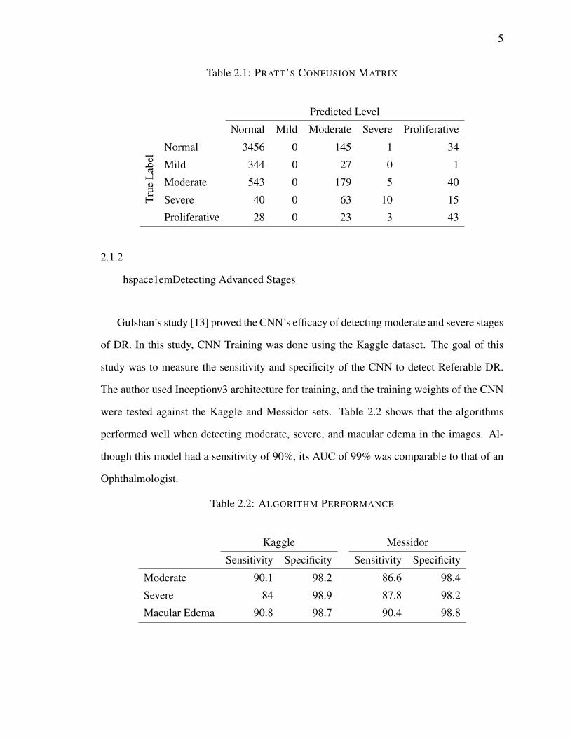
Gulshan’s study [13] proved the CNN’s efficacy of detecting moderate and severe stages
of DR. In this study, CNN Training was done using the Kaggle dataset. The goal of this
study was to measure the sensitivity and specificity of the CNN to detect Referable DR.
The author used Inceptionv3 architecture for training, and the training weights of the CNN
were tested against the Kaggle and Messidor sets. Table 2.2 shows that the algorithms
performed well when detecting moderate, severe, and macular edema in the images. Al-
though this model had a sensitivity of 90%, its AUC of 99% was comparable to that of an
Ophthalmologist.
Table 2.2: ALGORITHM PERFORMANCE
Kaggle Messidor
Sensitivity Specificity Sensitivity Specificity
Moderate 90.1 98.2 86.6 98.4
Severe 84 98.9 87.8 98.2
Macular Edema 90.8 98.7 90.4 98.8
6
2.1.3
hspace1emDetecting Early Stages
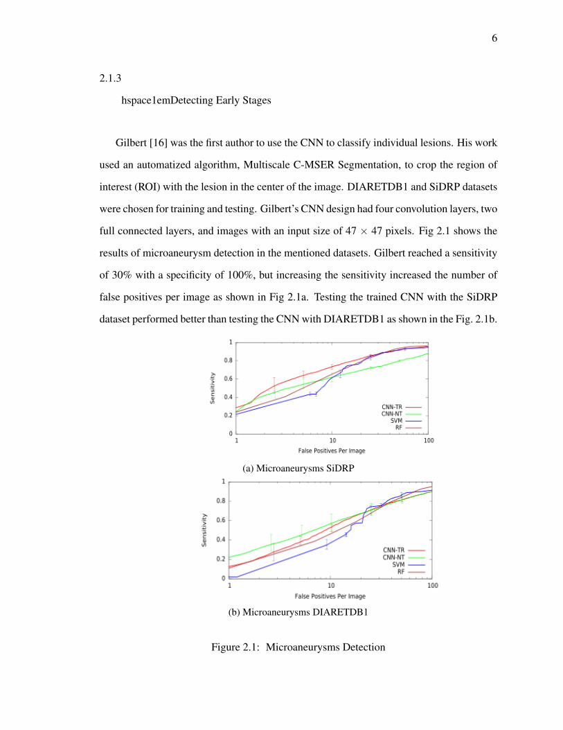
Gilbert [16] was the first author to use the CNN to classify individual lesions. His work
used an automatized algorithm, Multiscale C-MSER Segmentation, to crop the region of
interest (ROI) with the lesion in the center of the image. DIARETDB1 and SiDRP datasets
were chosen for training and testing. Gilbert’s CNN design had four convolution layers, two
full connected layers, and images with an input size of 47 × 47 pixels. Fig 2.1 shows the
results of microaneurysm detection in the mentioned datasets. Gilbert reached a sensitivity
of 30% with a specificity of 100%, but increasing the sensitivity increased the number of
false positives per image as shown in Fig 2.1a. Testing the trained CNN with the SiDRP
dataset performed better than testing the CNN with DIARETDB1 as shown in the Fig. 2.1b.
(a) Microaneurysms SiDRP
(b) Microaneurysms DIARETDB1
Figure 2.1: Microaneurysms Detection
7
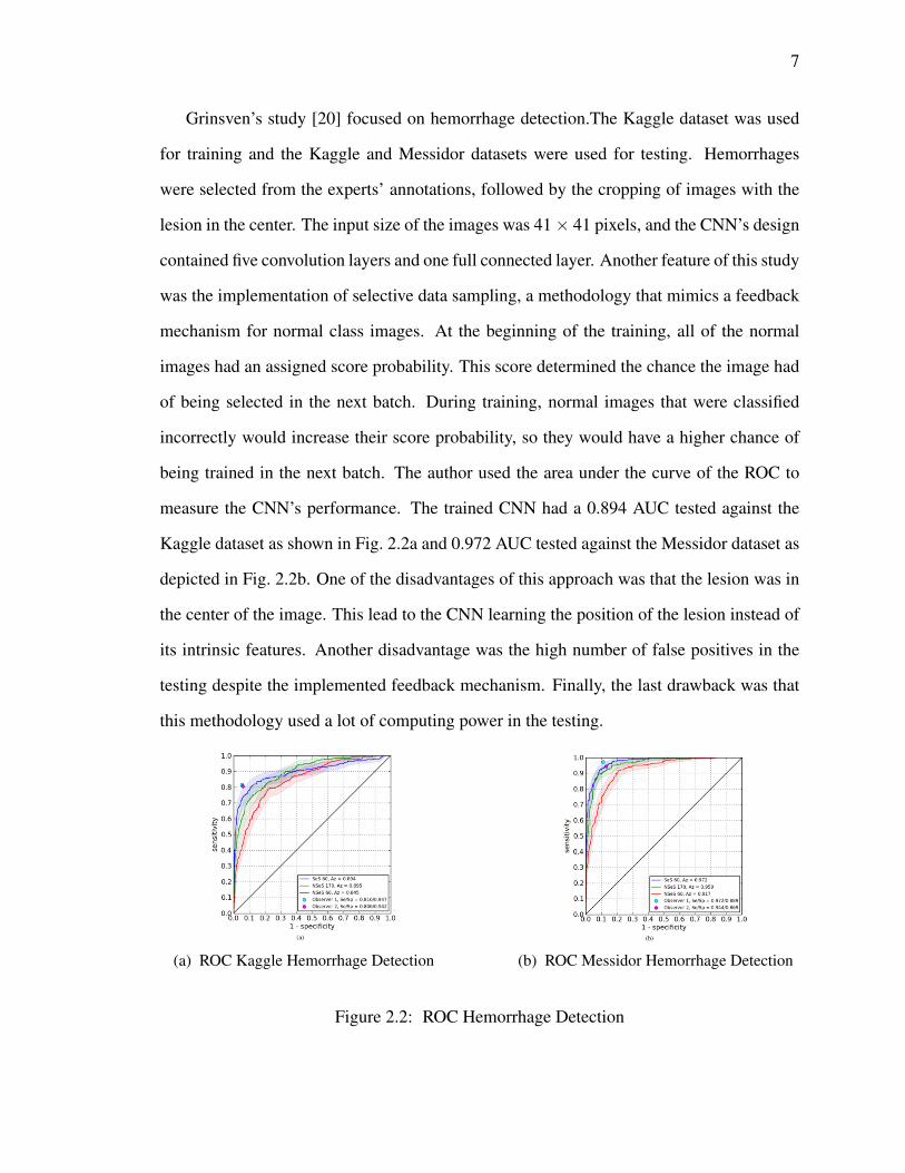
Grinsven’s study [20] focused on hemorrhage detection.The Kaggle dataset was used
for training and the Kaggle and Messidor datasets were used for testing. Hemorrhages
were selected from the experts’ annotations, followed by the cropping of images with the
lesion in the center. The input size of the images was 41× 41 pixels, and the CNN’s design
contained five convolution layers and one full connected layer. Another feature of this study
was the implementation of selective data sampling, a methodology that mimics a feedback
mechanism for normal class images. At the beginning of the training, all of the normal
images had an assigned score probability. This score determined the chance the image had
of being selected in the next batch. During training, normal images that were classified
incorrectly would increase their score probability, so they would have a higher chance of
being trained in the next batch. The author used the area under the curve of the ROC to
measure the CNN’s performance. The trained CNN had a 0.894 AUC tested against the
Kaggle dataset as shown in Fig. 2.2a and 0.972 AUC tested against the Messidor dataset as
depicted in Fig. 2.2b. One of the disadvantages of this approach was that the lesion was in
the center of the image. This lead to the CNN learning the position of the lesion instead of
its intrinsic features. Another disadvantage was the high number of false positives in the
testing despite the implemented feedback mechanism. Finally, the last drawback was that
this methodology used a lot of computing power in the testing.
(a) ROC Kaggle Hemorrhage Detection (b) ROC Messidor Hemorrhage Detection
Figure 2.2: ROC Hemorrhage Detection

8
2.2 Problem Definition And Proposed Solution
Microaneurysm detection in DR is a complex challenge. As mentioned in the previous
section, the difficulty of this task is determined mainly by the size of the lesions. The
last two studies tried to overcome this obstacle by cropping the image with the lesion in
the center without changing the resolution. Although these studies have an acceptable
sensitivity and specificity, the number of false positives is considerable. The following
example will explain the reason of having a high number of false positives: Having an
image size of 2000 × 2000 pixels will generate 2304 images with a size of 41 × 41 pixels,
so having a specificity of 90% will produce 231 false positive images with a size of 41 ×
41. Another important aspect in microaneurysm detection in DR is the quality of the image.
Although it is not mentioned in the review, some algorithms performed better when they
were tested with the Messidor dataset instead of the Kaggle dataset. It is known that the
Messidor dataset is a small dataset that has high quality images, while the Kaggle dataset
is the most important dataset, due to the size, with an acceptable quality. We hypothesized
that a good image pre-processing method would surpass this difficulty.
The aim of this study was to detect microhemorrhages of DR using Convolutional Neu-
ral Networks. We hypothesized that using two tests, one with high sensitivity and the other
with high specificity, would decrease the false positive rate. One test is a CNN trained with
an image that has a small size of 60 × 60 pixels, and the second test is a CNN trained with
an image that has a size of 420 × 420 pixels. While the first test will find all the lesions
in the images; the second test will better distinguish the difference between normal and
abnormal images.
During the study, other parameters would be measured such as the impact of augmen-
tation versus new input in accuracy and the use of a feedback mechanism.
9
CHAPTER 3
CNN REVISION
3.1 Introduction
Common tasks like asking your phone for directions, asking an electronic device to turn
on the AC, or asking your computer to read aloud a document is possible due to advances
in Machine Learning algorithms. The algorithms recognizing different patterns from the
input data [21] allow those devices to perform those tasks. One such algorithm is Artificial
Neural Networks (ANNs), which consists of layers of interconnected nodes (neurons). The
connections between these nodes have a dynamic value (weight) and each node performs
a summative function of their coming weights. Finally, a threshold function of the sum
of the weights determines the signal propagation of the nodes for the next layer. This
design tries to mimic the neuron connections in humans where inhibitory and excitatory
neurotransmitters will stop or propagate an electrical impulse [22, 23, 24]. In addition,
learning functions [25] were developed to modify the weights dynamically, making the
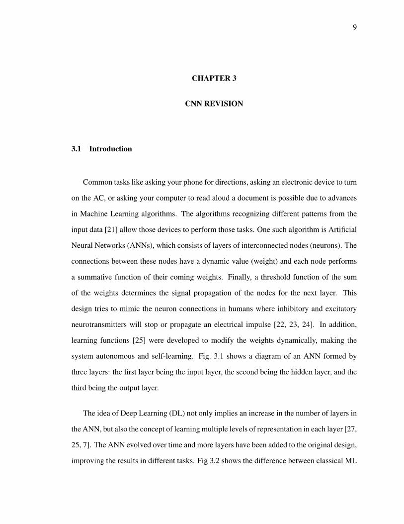
system autonomous and self-learning. Fig. 3.1 shows a diagram of an ANN formed by
three layers: the first layer being the input layer, the second being the hidden layer, and the
third being the output layer.
The idea of Deep Learning (DL) not only implies an increase in the number of layers in
the ANN, but also the concept of learning multiple levels of representation in each layer [27,
25, 7]. The ANN evolved over time and more layers have been added to the original design,
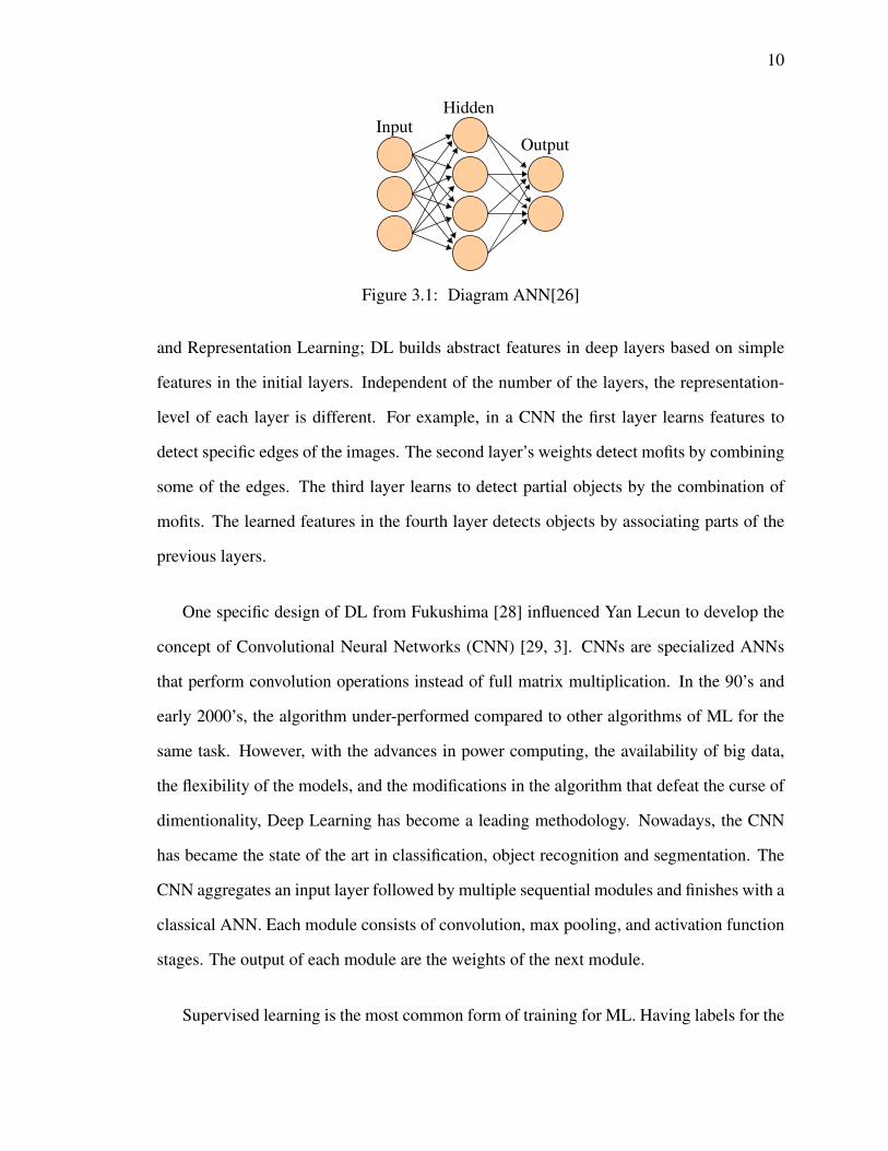
improving the results in different tasks. Fig 3.2 shows the difference between classical ML
10
Output
HiddenInput
Figure 3.1: Diagram ANN[26]
and Representation Learning; DL builds abstract features in deep layers based on simple
features in the initial layers. Independent of the number of the layers, the representation-
level of each layer is different. For example, in a CNN the first layer learns features to
detect specific edges of the images. The second layer’s weights detect mofits by combining
some of the edges. The third layer learns to detect partial objects by the combination of
mofits. The learned features in the fourth layer detects objects by associating parts of the
previous layers.
One specific design of DL from Fukushima [28] influenced Yan Lecun to develop the
concept of Convolutional Neural Networks (CNN) [29, 3]. CNNs are specialized ANNs
that perform convolution operations instead of full matrix multiplication. In the 90’s and
early 2000’s, the algorithm under-performed compared to other algorithms of ML for the
same task. However, with the advances in power computing, the availability of big data,
the flexibility of the models, and the modifications in the algorithm that defeat the curse of
dimentionality, Deep Learning has become a leading methodology. Nowadays, the CNN
has became the state of the art in classification, object recognition and segmentation. The
CNN aggregates an input layer followed by multiple sequential modules and finishes with a
classical ANN. Each module consists of convolution, max pooling, and activation function
stages. The output of each module are the weights of the next module.
Supervised learning is the most common form of training for ML. Having labels for the
11
Figure 3.2: Feature Discovering [27]
input allows the algorithm to compare the forward results of the CNN to the input labels
using a Cost Function. This function determines the distance (error) from the result of
the ANN and the image labels. Then the system adjusts the weights of the model using
learning algorithms like the stochastic gradient descendant (SGD). The weights in each
layer are adjusted using backpropagation before repeating a new cycle. The number of
cycles is not a constant and most researchers stop the training when overfitting is present,
which can be analyzed by looking at the accuracy curve for the training and validation sets.

12
3.2 Input And Output
Our input includes two dimensional (2D) arrays containing the intensity values between
0 to 255 for each channel (RGB). For example, in an image with a size of 420× 420 pixels,
the input is a three dimensional matrix (3D) of 420 × 420 × 3 pixels. The output is the
probability of the image belonging to a certain class.
3.3 Convolution
Convolution is a mathematical operation defined in the discrete form of two dimen-
sional images as follows:
s[i, ] = (I ∗K)[i, j] =∑m
∑n
I[m,n]K[i−m, j − n] , (3.1)
where x is the input, w is the kernel, and the output known as Feature Map. Convolu-
tions have three inherent characteristics to improve the ML algorithm: sparce interactions,
parameter sharing, and equivalent representation.
Sparce Interactions refers to the fact that using kernels with a size less than the input
size reduces the number of parameters. If we have an input with a size of 100 × 100 pixels
that it is fully connected to 10 hidden neurons, then we will have 100000 parameters plus
10 bias parameters. On the other side, a convolution with a kernel size of 3 × 3 × 20 has
180 parameters. Reduction in the number of parameters would diminish the computing
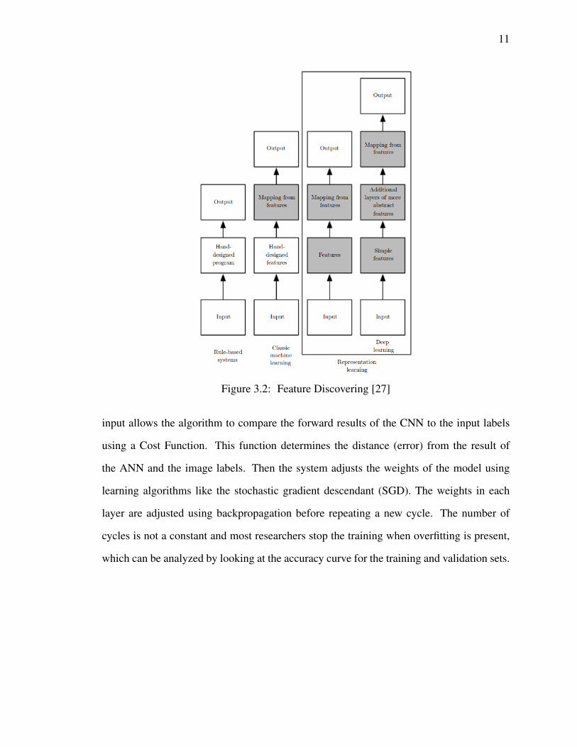
power needed to train the CNN. Another side effect of sparce interactions, is the pyramidal
structure of the receptive field which means deeper layers are influenced indirectly by the
upper layers as shown in Fig. 3.3
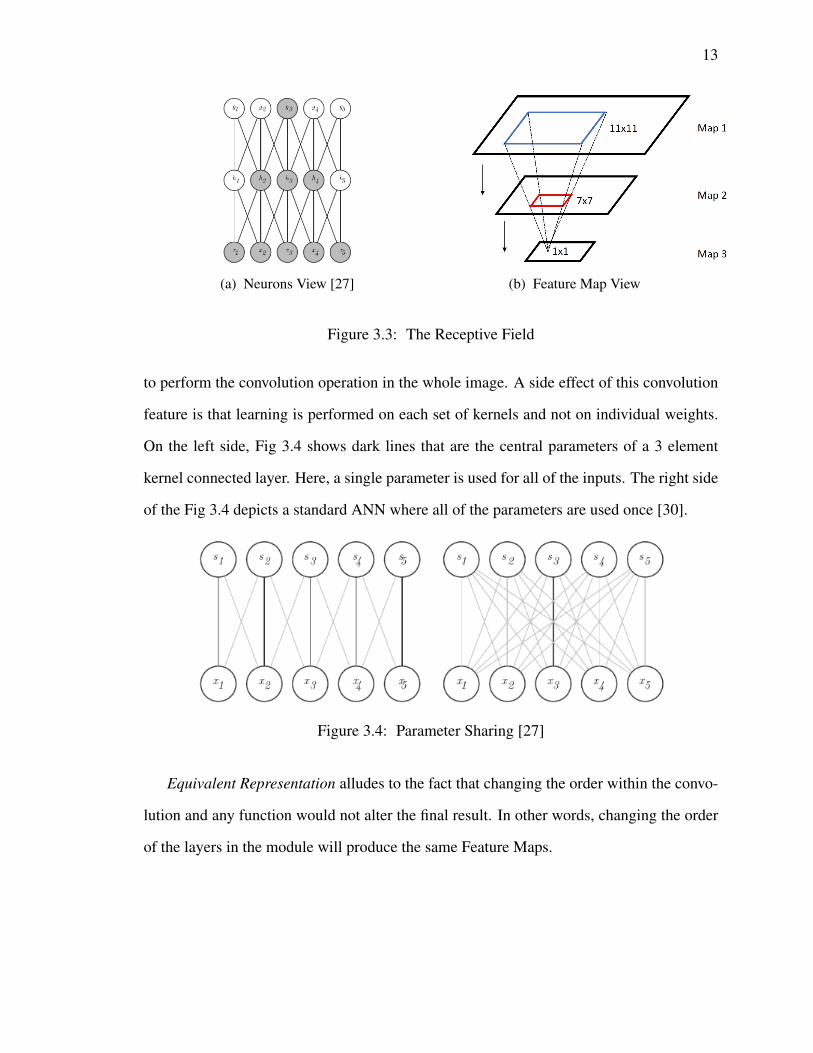
Parameter Sharing describes the use of the same parameters (the weights of the kernels)
13
(a) Neurons View [27] (b) Feature Map View
Figure 3.3: The Receptive Field
to perform the convolution operation in the whole image. A side effect of this convolution
feature is that learning is performed on each set of kernels and not on individual weights.
On the left side, Fig 3.4 shows dark lines that are the central parameters of a 3 element
kernel connected layer. Here, a single parameter is used for all of the inputs. The right side
of the Fig 3.4 depicts a standard ANN where all of the parameters are used once [30].
Figure 3.4: Parameter Sharing [27]
Equivalent Representation alludes to the fact that changing the order within the convo-
lution and any function would not alter the final result. In other words, changing the order
of the layers in the module will produce the same Feature Maps.
14
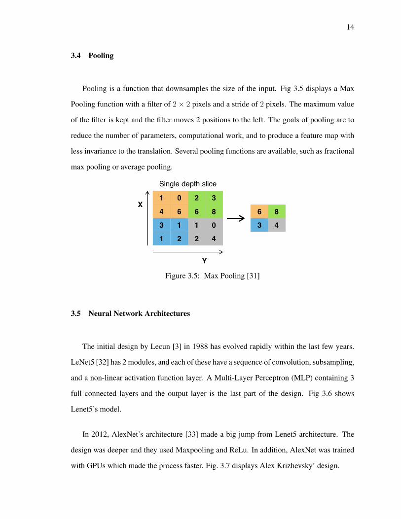
3.4 Pooling
Pooling is a function that downsamples the size of the input. Fig 3.5 displays a Max
Pooling function with a filter of 2 × 2 pixels and a stride of 2 pixels. The maximum value
of the filter is kept and the filter moves 2 positions to the left. The goals of pooling are to
reduce the number of parameters, computational work, and to produce a feature map with
less invariance to the translation. Several pooling functions are available, such as fractional
max pooling or average pooling.
Figure 3.5: Max Pooling [31]
3.5 Neural Network Architectures
The initial design by Lecun [3] in 1988 has evolved rapidly within the last few years.
LeNet5 [32] has 2 modules, and each of these have a sequence of convolution, subsampling,
and a non-linear activation function layer. A Multi-Layer Perceptron (MLP) containing 3
full connected layers and the output layer is the last part of the design. Fig 3.6 shows
Lenet5’s model.
In 2012, AlexNet’s architecture [33] made a big jump from Lenet5 architecture. The
design was deeper and they used Maxpooling and ReLu. In addition, AlexNet was trained
with GPUs which made the process faster. Fig. 3.7 displays Alex Krizhevsky’ design.
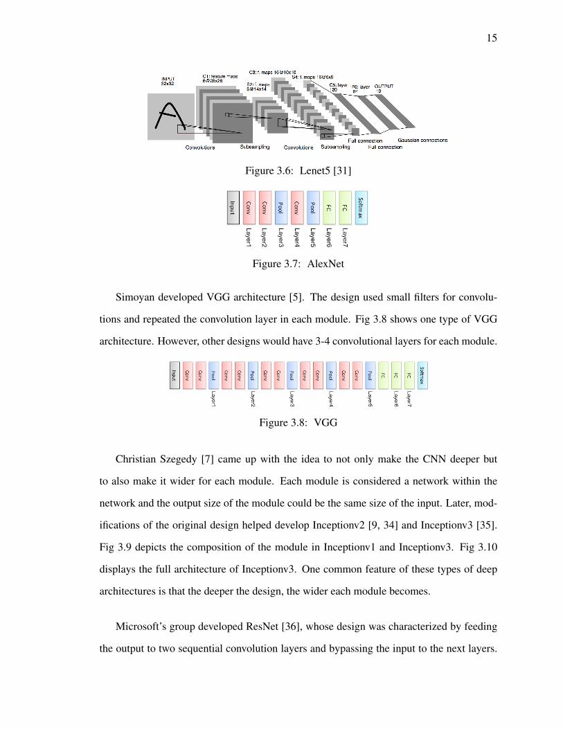
15
Figure 3.6: Lenet5 [31]
Figure 3.7: AlexNet
Simoyan developed VGG architecture [5]. The design used small filters for convolu-
tions and repeated the convolution layer in each module. Fig 3.8 shows one type of VGG
architecture. However, other designs would have 3-4 convolutional layers for each module.
Figure 3.8: VGG
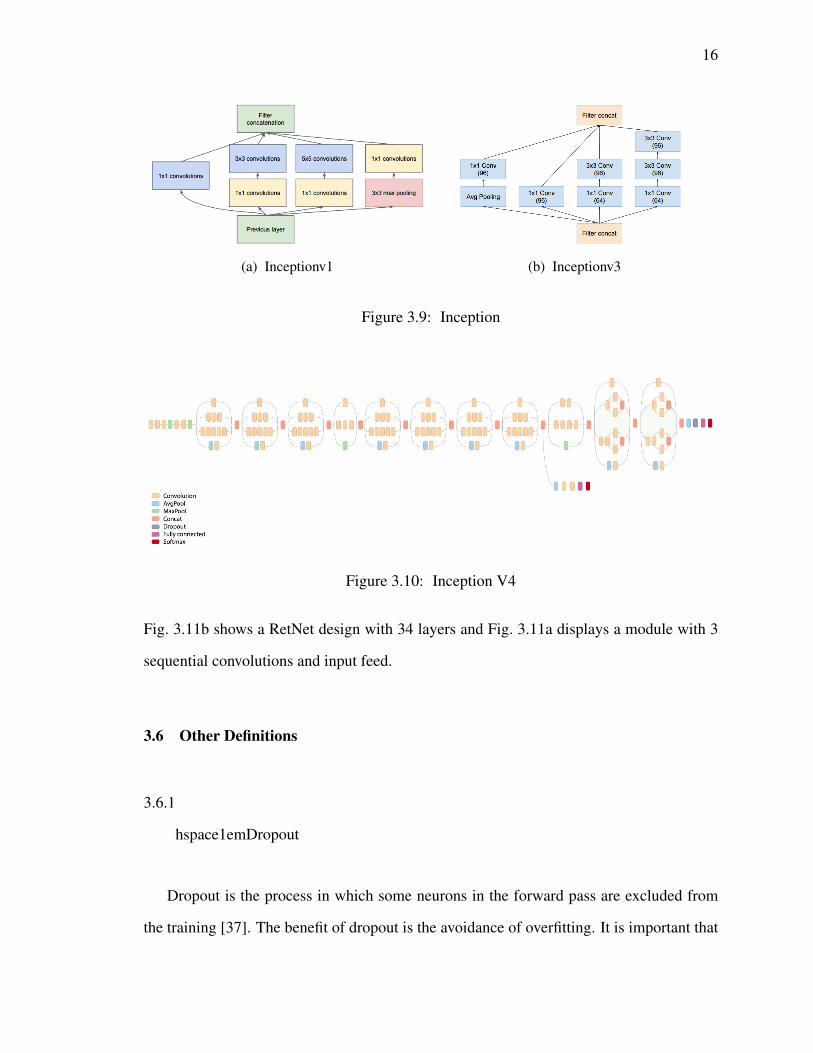
Christian Szegedy [7] came up with the idea to not only make the CNN deeper but
to also make it wider for each module. Each module is considered a network within the
network and the output size of the module could be the same size of the input. Later, mod-
ifications of the original design helped develop Inceptionv2 [9, 34] and Inceptionv3 [35].
Fig 3.9 depicts the composition of the module in Inceptionv1 and Inceptionv3. Fig 3.10
displays the full architecture of Inceptionv3. One common feature of these types of deep
architectures is that the deeper the design, the wider each module becomes.
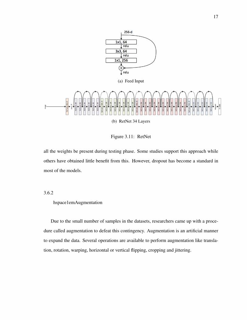
Microsoft’s group developed ResNet [36], whose design was characterized by feeding
the output to two sequential convolution layers and bypassing the input to the next layers.
16
(a) Inceptionv1 (b) Inceptionv3
Figure 3.9: Inception
Figure 3.10: Inception V4
Fig. 3.11b shows a RetNet design with 34 layers and Fig. 3.11a displays a module with 3
sequential convolutions and input feed.
3.6 Other Definitions
3.6.1
hspace1emDropout
Dropout is the process in which some neurons in the forward pass are excluded from
the training [37]. The benefit of dropout is the avoidance of overfitting. It is important that
17
(a) Feed Input
(b) RetNet 34 Layers
Figure 3.11: RetNet
all the weights be present during testing phase. Some studies support this approach while
others have obtained little benefit from this. However, dropout has become a standard in
most of the models.
3.6.2
hspace1emAugmentation
Due to the small number of samples in the datasets, researchers came up with a proce-
dure called augmentation to defeat this contingency. Augmentation is an artificial manner
to expand the data. Several operations are available to perform augmentation like transla-
tion, rotation, warping, horizontal or vertical flipping, cropping and jittering.
18
3.6.3
hspace1emReLu
ReLu is an activation function, that according to some studies, would prevent the van-
ishing gradient problem. The ReLu function, f(x) = max(0, x), is applied to the end of
each module, generally after pooling. The Leaked Rectifier Units (LeReLu) function is a
modification of the ReLu function in which the number 0 in max(0, x) is replaced by any
negative value.
3.6.4
hspace1emStride And Padding
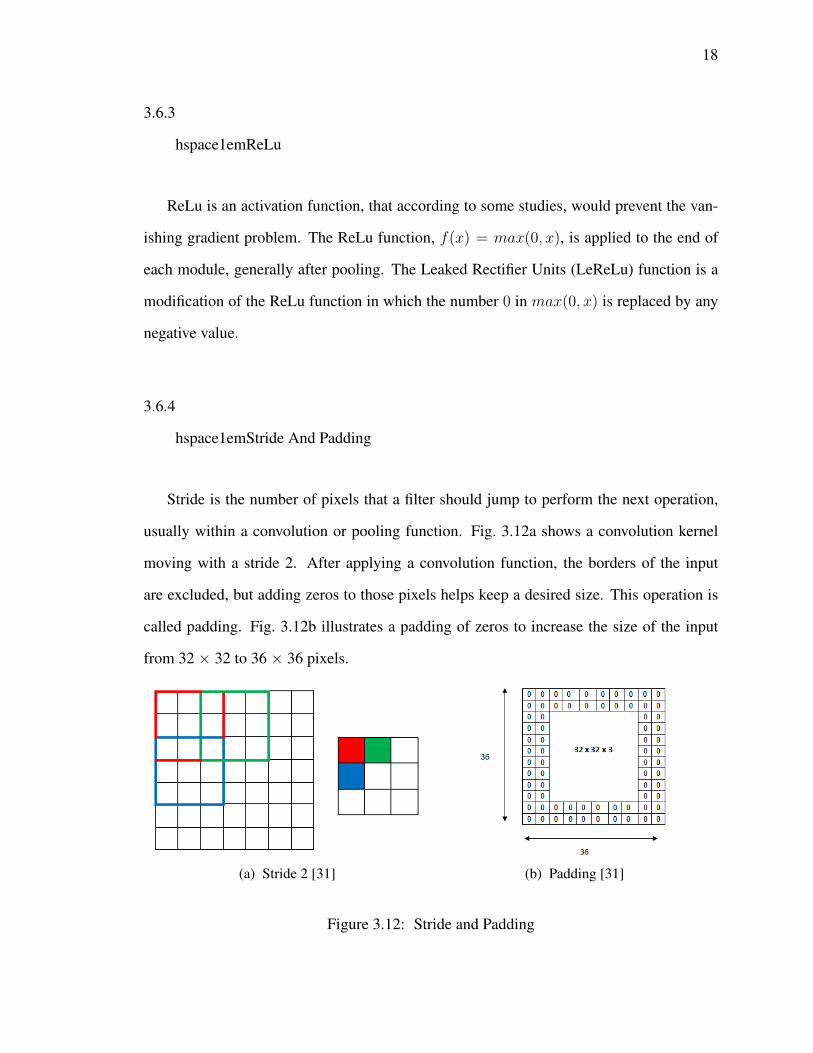
Stride is the number of pixels that a filter should jump to perform the next operation,
usually within a convolution or pooling function. Fig. 3.12a shows a convolution kernel
moving with a stride 2. After applying a convolution function, the borders of the input
are excluded, but adding zeros to those pixels helps keep a desired size. This operation is
called padding. Fig. 3.12b illustrates a padding of zeros to increase the size of the input
from 32 × 32 to 36 × 36 pixels.
(a) Stride 2 [31] (b) Padding [31]
Figure 3.12: Stride and Padding

19
CHAPTER 4
RESOURCES
4.1 Databases
The data sets utilized in this study are Kaggle diabetic-retinopathy-detection competi-
tion 1, Messidor datatabase 2, and the Diabetic Retinopathy Database and Evaluation Pro-
tocol 3.
4.1.1
hspace1emDataset Features
The majority of the available databases contain DR images of all classes. However, be-
cause the aim of our study is to detect microaneurysms, and to differentiate images with and
without lesions, we chose images that only belong to class zero, one, and two (Messidor).
i. Kaggle Dataset: Eyepacs provided the images to Kaggle, where we accessed them
and used them in our study. This dataset implements the Clinical Diabetic Retinopa-
thy Scale to determine the severity of DR (none, mild, moderate, severe, prolifer-
ative) and contains 88702 fundus images. Table 4.1 shows unbalanced data with
prominent differences between mild and normal classes. It is also evident that most
of the images belong to the testing set.
1https://www.kaggle.com/diabetic-retinopathy-detection2Kindly provided by the Messidor program partners (see http://www.adcis.net/en/DownloadThirdParty/Messidor.html)3http://www.it.lut.fi/project/imageret
20
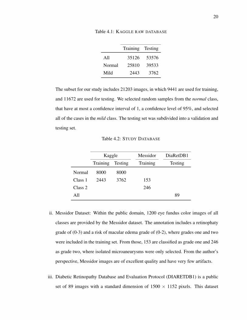
Table 4.1: KAGGLE RAW DATABASE
Training Testing
All 35126 53576
Normal 25810 39533
Mild 2443 3762
The subset for our study includes 21203 images, in which 9441 are used for training,
and 11672 are used for testing. We selected random samples from the normal class,
that have at most a confidence interval of 1, a confidence level of 95%, and selected
all of the cases in the mild class. The testing set was subdivided into a validation and
testing set.
Table 4.2: STUDY DATABASE
Kaggle Messidor DiaRetDB1
Training Testing Training Testing
Normal 8000 8000
Class 1 2443 3762 153
Class 2 246
All 89
ii. Messidor Dataset: Within the public domain, 1200 eye fundus color images of all
classes are provided by the Messidor dataset. The annotation includes a retinophaty
grade of (0-3) and a risk of macular edema grade of (0-2), where grades one and two
were included in the training set. From those, 153 are classified as grade one and 246
as grade two, where isolated microaneurysms were only selected. From the author’s
perspective, Messidor images are of excellent quality and have very few artifacts.
iii. Diabetic Retinopathy Database and Evaluation Protocol (DIARETDB1) is a public
set of 89 images with a standard dimension of 1500 × 1152 pixels. This dataset

21
also includes ground truth annotations of the lesions from four experts, which are
labeled as small red dots, hemorrhage, hard exudates, and soft exudates. We parsed
the xml files with the annotations, to get the coordinates of the small red dots and
hemorrhages. This set will be used for testing purposes.
Table 4.2 shows the number of images per class in each database used in the study.
4.2 Image Annotations
The main author of this study, a medical doctor and General Surgeon, was the person
who located and annotated the microaneurysms in the images that belong to class one and
two. The range of difficulty to localize these lesions varies, but for the purpose of this study
the authors chose only the evident lesions from these images, leaving dubious images out
of the study. Some pictures have more than one microaneurysm and each is counted as
different in this study.
4.3 Machine Learning Framework
Torch 4 was the framework chosen for this study and the multi-gpu Lua scripts 5 were
adapted to run the experiments. Other frameworks used in this study include OpenCV for
imaging processing, R-Cran for statistical analysis and plotting and Gnuplot for plotting.
The training of the CNNs was performed on a 16.04 Ubutu Server with four Nividia M40
GPU’s using Cuda 8.0, and Cudnn 8.0.
4http://torch.ch/5https://github.com/soumith/imagenet-multiGPU.torch
22
CHAPTER 5
METHODS USED TO IMPLEMENT OUR PROPOSED SOLUTION
An improved image was created for the annotations by applying an original pre-processing
approach. Once the author selected the coordinates of the lesions, the cropping of the im-
ages with the lesions and the cropping of normal fundus images was executed. Two datasets
with cropped sizes of 60x60 and 420x420 were obtained and trained using modified CNNs.
One of our modifications included a novel feedback mechanism for training. We also eval-
uated the increase in the size of the dataset by using either augmentation or adding new
images. Receiver Operating Characteristics (ROC) [38] was used to get the cut-off of the
predicted values in order to obtain a more accurate sensitivity and specificity of the models.
Lastly, an analysis on the more precise model with the DiaRetDB1 was performed to find
its overall sensitivity.
5.1 Processing Images
Batch transformations on the lightness and color of the images were used to produce
higher quality images for annotations and a comparative analysis of using CNNs with in-
puts of images with and without pre-processing was performed.
Initially, the images were trimmed to eliminate the black border, which did not add
any value; on the contrary, it only added noise to the study’s purpose. Then, the descrip-
tive statistics were calculated and K-means analysis was used to divide the images in three
groups (dark, normal, and bright). A function based on the statistics was performed to
23
transform the lightness of the images using LAB color space. After collecting the a∗ and
b∗ intensity values in the LAB color space from vessels, microaneurysms, hemorrhages,
and a normal background, a Support Vector Machine (SVM) was used to separate microa-
neurysms and hemorrhages from the background. Based on the SVM, another function
used to reduce the color of the image based on the LAB color space was created.
5.1.1
hspace1emGetting Images Statistics
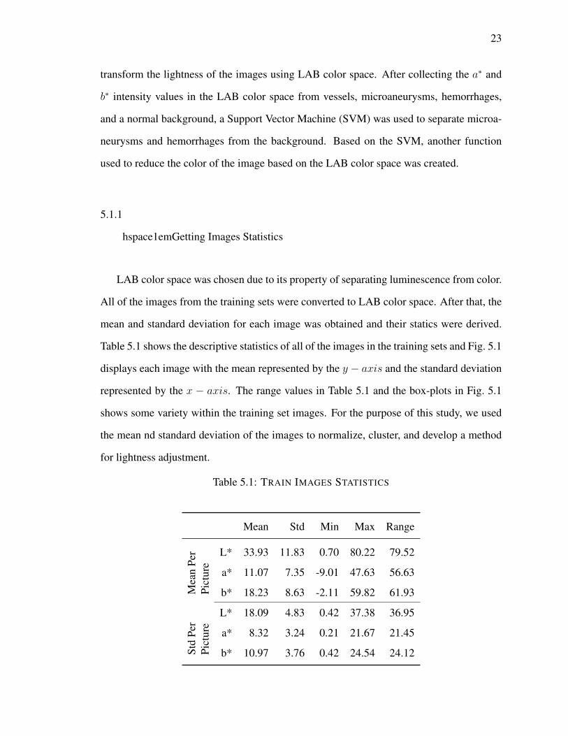
LAB color space was chosen due to its property of separating luminescence from color.
All of the images from the training sets were converted to LAB color space. After that, the
mean and standard deviation for each image was obtained and their statics were derived.
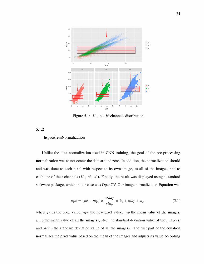
Table 5.1 shows the descriptive statistics of all of the images in the training sets and Fig. 5.1
displays each image with the mean represented by the y − axis and the standard deviation
represented by the x − axis. The range values in Table 5.1 and the box-plots in Fig. 5.1
shows some variety within the training set images. For the purpose of this study, we used
the mean nd standard deviation of the images to normalize, cluster, and develop a method
for lightness adjustment.
Table 5.1: TRAIN IMAGES STATISTICS
Mean Std Min Max Range
Mea
nPe
rPi
ctur
e
L* 33.93 11.83 0.70 80.22 79.52
a* 11.07 7.35 -9.01 47.63 56.63
b* 18.23 8.63 -2.11 59.82 61.93
Std
Per
Pict
ure
L* 18.09 4.83 0.42 37.38 36.95
a* 8.32 3.24 0.21 21.67 21.45
b* 10.97 3.76 0.42 24.54 24.12
24
0
20
40
60
80
0 10 20 30
StdM
ean a*
b*
L*
●●
●●
●●
●●
●●●● ●
●●
●
● ●●
●
●●
●
●●●
●●
●
●
●●
●
●
●●
●●
●
●
●
●
● ●
●●
●
●
●●
●
●
●
●
●
●
●●
●
●●
●●
●
●
●●●●
●
●
●
●●
●●
●
●
●●
●
●
●
●●
●●●●●●
●●
●
●●●
●
●
●●
●●
●●
●●
●●
●
●
●
●
●●●●
●●●
●
●
●
●
●
●
●●
●●●
●●
●●
●
●
●
●
●●
●
●
●●●
●
●● ●●
●●
●●●●●
●
●●
●
●●
●●
●
● ●●
●
●
●
●
●●●
●
●
●●
●●●
●●
●
●●
●●
●
●
●●
●
●
●●
●●
●
●●
●●
●
●●●
●
●
●
● ●
●
●
●
●
●●
●●●
●
●
●●●
●●
●●
●
●●●
●●●
●●
●
●
●●●
●●
●●
●●
●
●●●●
●
●
●
●●●
●
●
●
●●
●●●
●
●
●
●
●
●
●
●●●
●
●●●
●
●●●
●●
●
●
●
●
●●
●
●
●
●●
●●●
●●
●
●
●
●
●●
●●
●
●●
●●●●
●
●●
●●
●●
●
●
●
●●
●
●
●
●●
●●
●●●
●●
●
●
●
●● ●●
●
●
●
●
●
●
●
●
●
●
●
●● ●
●
●●
●
●
●●
●
●
●
●●
●
●
●
●●
●●●
●●
●
●
●●●
●
●
●
●●●
●●
●●●
●
●
●
●●
●●
●
●●
●
●
●●
●
●
●●
●
●●
●
●
●●●
●
●
●
●●●
●●
●
●
●●
●●
●
●●
●●
●
● ●●●
●●
●
●
●
●
●
●
●
●
●●●●●●
●
●●
●●
●
●
●●●●
●
● ●
●
●
●
●●
●
●
●●
●
●
●●
●●●●●
●
●
●
●●●
●
●●
●
●
●
●●●●
●
● ●●
● ●
●
●
●●
●
●●
●●●
●●
●
●●
●●
●
●●●● ●●
●
●
●
●
●●
●
●●
●●●●
●●
●
●●●●
●
●
●
●●
●●
●●
●●●●
●
●
●
●●
●●●
●
●●
●●
●
●●
●
●
●
●●
●
●●●●
●●●
●●
●●
●●
●
●
●●
● ●●●●
●
●●
●
●
●●●
●
●
●●
●
●
●●●●
●
●
●●●
●
●
●
●●
●
●
●●
●
●
●
●
●
●
●●
●
●●●
●
●●
●
●
●●
●
●
●
●●
●
●●
●
●
●
●●
●
●
●●
●●
●●
●
●
●
●
●
●●●●●
●●●
●●●
●
●
●
●●●
●
●
●
●
●
●
●●
●●
●
●
●● ●
●
●
●
●
●●
●●
●
●
●
●●●
●
●
●
●
●
●●●
●
●●
●●
●
●
●●●●
●
●●
●●
●
●●●
●●
●●
●
●●
●
●
●
●
●
● ●●
●
●●
●●
●●
●●
●
●●
●●
●
●
●
●●
●
●
●
●
●
●
●
●●
●
●●
●●
●●
●●
●
●
●●●
●
●
●●
●●
●
●
●●●
●
●●
●
●●
● ●
●
●
●●
●
●
●●
●
●
●
●
●●
●
●●
●●●●
●
●
●
●
●●
●
●
●
●
●●●
●
●
●
●
●
●●
●
●●
●●●
●
●
●●
● ●
●
●
●
●●
●
●●
●●
●●
●
●
●
●●
●
●
●
●●
●
●
●
●
●● ●
●●
●●●
●●
●●
●
●
●
●
●
●●
●
●
● ●●●
●●
●
●●
●●
●●
●●
●
●
●●
●●●
●●
●●
●
●
●
●
●
●
●●
●●
●●
●●
●●
●
●●
●●
●
●●●
●
●
●
●
●●
●●
●●
●●
●●
●
●
●
●
● ●
●
●
●
●
●
●
●●
●●
●
●
●●●
●●
●
●●
●
●●
●●
●●
●
●●●●
●
●●
●
●●
●
●
●
●
●
●
●
●
●
●● ●
●●
●
●●
●
●
●
●
● ●●●
●●●
●
●●
●
●
●●
●
●
●●
●
●
●●●
●●
●
●●
●
●
●●
●
●●
●
●
●
●
●
●
●●●
●
●
●
●●
●
●●
●●
●●
●●
●
● ●
●
●
●
●
●
●
●●
●
●
●
●●
●●
●●
●●
●
●
●
●
●
●●
●●
●
●●●●
●
●●●●
●
●
●
●
●
●
●●●●
●●
●
●●●
●
●
●●
●
●
●
●●
●
●● ●
●
●
●●
●
●●
●●
●●
●
●●
●
●
●
●
●
●●
●
●●●●
●
●●
●
●
●●
●
●●
●
●●
●
●●
●
●●●●
●●
●
●
●●
●●
●●
●
●
●
●●
●●
●●
●●●
●
●
●
●
●●
●
●
●
●
●
●
●●
●
●
●
●●●●
●
●
●
●
●
●● ●
●
●●●●
●●
●
●●
●●●
●
●●●●
●
●
●●●
●●●●●
●
●
●●
●●
● ●
●
●
●
●●
● ●●
●
●
●
●● ●●●
●●
●
●●
●●
●●
●
●
●
●●
● ●●
●
●●
●●
●●
●●
●●
●
●
●
●
●●
●●●●
●
●●
●●
●
●
●●●
●
●
●●
●
●●
●
●●
●
●
●●
●●
●
●
●
●
●●
●
●●
●
●●
●
●●
●
●●
●
●
●
●●●
●●
●
●●
●●
●
●
●●●
●
●
●
●●
●
●●
●
●
●●
●
●
● ●●
●●●
●
●
●
●
●
●●
●
●
●
●
●
●
●●
●●
●
●●
●
●
●
●
●●
●
●
●●●●●
●●
●
●
●
●●●
●●
●●●
●●
●●
●
●●
●●
●
●●
●
●●
●
●●●
●●
●
●
●●
●●
●
●
● ●● ●●
●●
●
●
●●
●
●
●
●
●
●●●
●
●
●●
●●●●●
●
●
●
●
●
●
●●●
●
●●
●
●
●●●
●●
●
●
●●
●●
●
●
●
● ●●●
●
●●
●
●
●●
● ●
●
●
●
●
●
●
●
●
●
●●
●
●●
●●●
●●
●●●
●●
●
●
●●
●
●
●
●
●
●
●
●
●
●
●●
● ●
●●
●
●●
●●
●
●●
●
●●
●●
●●
●
●●
●
●●
●●
●
●●
●
●●
●
●
●●●●
●
●
●
●●●
●
●●
●
●●●
●●
●●
●
●
●
●●●●
●
●●●
●
●● ●
●
●
●
●
●
●●
●
●
●
●
●
●
●●
●
●
●
●
●
●●
●●●
●
●
● ●
●
●
●
●
●
●
●●●
●
●●●●
● ●●
●
●
●
●●
●●●●
●
●●●
●
●●
●
●
●
●
●
●
●
●●
●
●
●
●
●
●
●
●●●●
●●
●●
●
●
●
●
●
●
●
●
●
●●
●●●●
●●
●●●●●
●●
●
●●
●
●●
●●
●●●
●●
●●
●●●
●●
●●
●●
●●
●
●●
●●
●
●
●●
●●
●●●
●
●
●●
●●
●●
●●
●
●● ●
●
●
●
●
●●
●
●●
●●●●
●
●●
●●●
●
●
●●●
● ●
●●
●
●●
●
●
●
●
●
●●●
●●
●
●● ●●
●
●●
●
●●●
●
●
●
●
●●
●
●●
●●●●
●●●
●
●
●●
●●
●●●
●
●
●●
●●
●●
●●
●
●
●
●
●
●
●●
●
●●
●
●
●
●
●
●
●●
●●
●
●
●●
●
●
●
●
●●●
●●●
●
●
●
●●●
●
●●
●
●
●●●●
●
●● ●
●●
●●
●●
●●
●
●
●●
● ●
● ●
●●
●
●
●●
●
●
●●
●
●
●●
●
●●
●●
●
●
●●
●
●●
●
●
●●●
●●
●●
●●●
●●
●●
●
●
●●
●●
●●
●●
●
●●
●●
●●●
●
●●
●
●●
●
●
●
●
●●
●
●
●
●●
●
●
●
●●● ●
●●
●
●
●●
●●●●●
●●
●
●
●●
●
●
●
●●
●●
●●
●●
●●
●
●
●●●
●●
●
●●
●
●●●
●
●
●
●
●●
●
●
●●
●
●
●
●
●
●●
●●●
●●
●●
●
●●
●●
●● ●
●●
●●
●
●
●● ●
●●
●●●
●●
●●
●
●●
●
●●
●●
●
●●●
●
●●
●●●
●
●
●
●
●
●●
●●
●
●●
●
●
●●
●●●
●
●●
●
●
●
●●
●●
●●●●
●●
●
●●
●●
●
●
●●●
●●
●
●
●
●●
●
●
●
●●●
●
●●
●●●
●●
●●●● ●
●
●●
●●●
●●●●
●
●
●
●●
●
●●●
●
●
●
●
●●
●●
●
●
●
●
●●
●●
●●●
●
●
●
●●
●●● ●
●●
●
●●
●
●●
●●
●●
●
●●●●
●●
●●
●●
●●
●
●
●●
●
●●
●●
●●
●
●●●
●
●●
●
●
●
●
●●
●
●
●●
●
●
●
●
●●
●
●●
●●
●●
●
●●
●
●●
●●
●
●
●●●●
●
●
●
●●
●
●
●●
● ●
●
●
●●
●
●●
●
●
●●
●
●
●●
●
●
●
●
●
●
● ●
●●
●
●
●●
●
●
●
●
●
●●
●●
●●
●●
●
●
●●
●
●
●
●
●
●●
●●
●●
●
●
●●
●
●●
●●
●●
●●
●
●●●
●●
●
●
●
●●
●
●●●
●
●●
●
●
●
●
●●
●●●
●●
●
●●●
●
●
●●
●●
●
●●
●
●
● ●
●
●
●●
●
●
●●●
●●●
●
●
●●
●●
●●●
●
●●
●
●
● ●
●
●
●●
●
●
●
●
●
●
●●
●
●
●●
●
●●
●●
●
●●
●●
●
●●
●
●●
●●
●
●
●
●●
●
●
●
●
●
●
●
●
●
●●
●
●
●
●
●●
●●
●
●
●
●
●●
●
●●
●
●
●
●●
●
●
●●●
●
●
●●
●
●●●
●
●●
●
●●
●●
●●
●
●
●
●●
●
●●●●
●
●
●
●
●●
●
●
●
●
●
●●
●●
●●
●
●
●
●
●
●
●●
●
●●
●
●
●
●
●
●●●
●●
●
●
●
●
●●
●●
●
●
●
●
●●
●
●
●●
●●
●●
●
● ●●
●
●
●
●●
●
●
●
●
●
●
●●
●
●
●
●●
●
●● ●
●●
●
●
●
●●
●
●●● ●●
●●
●
●
●●
●
●
●●●
●
●
●
●●
●●●
●●
●
●
●●●
●●
●
●●●
●●
●
●●
●
●●●
●●●
●
●●
●
●
●●
●
●●●
●
●●
●
●
●●
●
●
●
●
●
●●
●
●
●
●
●●
●
●
●
●
●
●●
●●
●●●
●●
●
●
●
●
●
●
●
●
●●
●
●
●
●●
●●●●
●
●
●
●●●
●
●
●
●
●
●
●●
● ●
●●
●
●
●●●●
●●
●●
●
●
●
●●●
●
●
●
●
●
●
●
●
●
●
●
●
●
●
●
●
●
●●
●
●●
●
●●
●
●
●
●●
●●
●
●
●
●
● ●
●
●
●
●
●
●●
●
●●
●●
●
●
●
●
●
●●●
●
●
●
●
●
●●
●
●
●
●
●●
●●
●●
●
●
●
●
●
●
●
● ●●
●
●●
●
●
●
●
●
●
●
● ●●
●
●
●
●●
●●
●●●
●●
●
●●
●●●
●
●
●
●
●
●
●
●
●
●
●●
●
●
●●●
●
●
●
●●
●
●
●
●
●●
●
●
●●
●
●
●
●
●
●
●●
●
●●
●●
●
●●●
●
●
●
●
●
●●
●
●●
●
●
●
●
●
●
●
●●
●
●
●
●
●
●
●●●
●●
●
●
●
●●
●
●●●
●
●
●
●
●●
●
●
●
●
●
●
●●
●●
●
●
●
●●●
●
●
●
●●●●●
●
●
●
●
●
●
●
●
●
●
●
●
●
●
●●
●●
●
●
●
●
●
●
●●●
●●
●
●●
●
●
●
●●
●
●●●
●
●
●
●●●
●●●
●●
●
●
●
●●
●
●●
●●
●
●
●
●●
●
●
●
●
●●
●
●
●
●
●●
●●●●
●●
●
●●●
●
●
●●
●
●●
●
●
●
●
●
●
●
●
●
●●
●
●
●
●
●●
●●●
●
●
●
●
●
●●
●●●
●
●
●
●
●
●
●
●
●●
●●
●
●
●
●●●
●
●●
●
●
●
●
●●
●
●●
●
●
●●●●
●
●
●
●
●
●
●
●
●●
●●
●
●
●
●
●
●
●●●
●
●
●
●
●
●
●
●●●
●●●
●●
●●
●
●
●
●●
●●
●
●
●
●
●
●
●●
●
●●
●
●
●
●
●●
●●
●●
●●●
●
●
●●
●
●
●
●
●
●
●●●●
●●
●
●
●
●
●
●●
●●
●●
●●
●
●●
●
●
●
●●
●
●
●
●●
●
●
●
●
●
●●
●
●
●●
●
●●●
●●
●
●
●
●
●
● ●
●
●●
●
●
●
●●
●●
●
●●●●●●●
●
●●
●
●●
●
●●
●
●
●
●●
●
●●
●
●
●
●
●
●
●
●
●
●
●
●
●●
●
●●
●
●
●●●
●
● ●
●●
●●●
●●
●
●●
●●
●●
●
●●
●
●
●●
●
●
●●
●
●
●
●
●●
●●●
●●
●●
●
●●
●
●
●●
●
●●
●●●●
●
●
●●
●
●
●
●
●●
●●
●●
●
●
●
●●
●
●●
●
●
●
●●●●●
●●
●
●
●
●
●●
● ●●
●
●
●●●
●
●
●
●
●●
●●
●
●
●●●
●
●
●
●
●●
●●
●●
●
●●
●
●
●
●
●
●●
●●●
●●
●●
●
●●
●●●●●
●
●
●
●
●●
●
●●
●●
●●
●
●
●
●
●
●●●
●●
●●● ●
●●●
●
●
●
●●
●
●
●●
●
●
●
●
●
●●
●
●
●
●
●
●
●
●
●
●
●
●
●
●●
●
●
●
●●●
●●
●
●●●●●
●
●
●●●
●
●
●●
●
●●●
●
●
●
●
●●
●
●
●
● ●
●
●●●
●●
●
●
●
●
●
●
●
●●
●
●●
●●
●●●●
●
●
●●
●
● ●
●
●
●
●
●●
●●
●●
●
●
●
●●●●●
●●●
●
●
●●
●
●
●
●
●●
●
●
●
●
●
●
●
●
●
●
●
●
●
●●
●
●
●
●
●
●
●
●
●●
●
●
●●
●●●
●
●
●●
●
●
●
●●
●●●
●●
●●
●
●
●●
●●
●
●●
● ●
●●
●
●
●●
●
●
●
●
●
●
●●
●
●
●
●
●
●
●
●
●
●
●
●●
●●
●
●
●
●●●
●
●
●
●
●
●
●
●
●
●●
●●
●●
●●
●
●●●●
●●
●
●
●●
●
●
●●
●●
●
●
●●
●●
●
●
●
●
●●
●
●
●●
●
●
●
●●
●●
●
●
●●
●
●
●●
●
●
●
●●
●
●●●
●
●
●
●●
●●●●
●
●
●
●
●
●
●
●
●
●●
●
●
●●
●●●
●
●
●●●
●
●
●●●
●●●
●●●●
●
●●
●●
●
●
●
●
●●
●
●
●
●●
●
●●
●●
●●
●●
●
●
●
●
●●
●●
●
●
●
●
●
●
●
●●
●
●●
●
●
●●
●●
●
●
●
●
●●
●●
●
●●
●
●
●
●
●
●
●●
●● ●
●
●●●●
●
●
●
●
●
●●
● ●
●
●
●
●
●●
●
●
●● ●●
●●
●
●
●●
●●●
●
●●●
●
●●●
●
●
●
●●
●
●
●
●
●●●
●
●●
●●●
●
●
●
●
●
●●● ●
●●
●
●
●
●●
●
●
●●
●
●●
●
●
●
●
●
●
●
●
●●
●
●●●
●
●
●●●
●●
●
●
●
●
●
●
●
●●
●●
●
●
● ●●
●
●●
●
● ●
●●
●
●
●
●
●
●
●
●
●
● ●
●●●
●
●
●
●
●●
●●
●
●
●
●●
●
●●
●
●
●●●
●
●●
●
●●
●
●●
●
●
●●●●
●
●●
●●
●
●
●●
●●
●
●
●
●
●
●●●●
●●
●●
●
●
●●
●
●
●
●
●●
●
●●
●●
●●
●
●●
●●
●●
●
●
●●●●
●
●
●
●●
●
●
●
●
●
●
●
●
●●
●
●●
●
●
●
●●
●
●●
●
●
●
●
●
●
●●●
●
●●
●
●
●
●●
●●
●●
●●
●
●
●
●
●
●●
●●
●●
●●●
●
●●
●
●
●●
●
●●
●●●
●
●
●
● ●
●●
●●
●
●
●
●
●
●
●●
●
●
●
●●●
●
●
●
●
●
●●
●
●●●●●
●
●
●●
●●
●●
●●
●
●
●
●
●●
●
●●
●
●●●
●●●
●
●
●●●●
●
●●
●●
●●
●
●
●
●
●
●
●●
●●●●
● ●
●
●
●●●
●●
●●
● ●
●●●●
●●
●●
●
●
●●
●
●●
●
●
●●
●●●
●
●
●
●●
●
●
●
●●
●
●
●
●●●●
●
●
●
●
●
●●
●●
●
●●
●
●
●
●
●●
●
●
●
●●
●●
●●
●
●●
●
●
●●●●●●
●
●
●
●
●
●
●
●
●
●●
●
●
●
●
●●
●
●
●
●
●
●●
●●●
●●
●
●
●
●●
●●
●
●●
●●
●
●
●
●
●●●●●
●●
●●●
●●
●
●●
●
●●
●●
●
●● ●
●
●●
●●
●
●
●
●
●
●
●●
●●
●
●
●
●
●
●
●
●
●●
●
●●●
●
●
●
●●
●
●
●
●●
●
●
●●
●●
●
●
●
●●●
●
●●
●
●
●●●
●
●
●●
●●
●
●
●● ●
●
●●
●●
●●
●
●●
●
●●
●
●
●
●
●
●
●
●●
●●
● ●
●
●●
●
●●
●
●●
●●●
●●
●●●
●
●●
●
●
●●
●
●●
●●
●
●
●
●
●●
●●
●
●●
●●●
●
●●●
●
●
●●
●
●●
●
●●
●
●●
●
●
●
●
●●
●●
●
●●
●
●
●
●
●
●●●
●●
●
●
●
●
●●
●
●●
●
●
●●
●
●●
●
●●●●
●
●
●●
●●
●
●
●
●●
●
●
●
●
●
●
●
●
●●
●
●
●
●●
●●
●
●
●●
●●
●●
●
●
●
●●●
●
●
●
● ●●
●
●
●
●
● ●●
●●
●
●
●
●
●
●
●
●
●
●
●
●●
●
●
● ●
●
●●
●
● ●
●
●●
●
●
●●
●
●
●
●
●
●
●●
●
●●
●●
●
●
●
●●
●
●●
●●●
●
●
●
●●
●
●
●●
●
●
●
●
●
●
●
●●
●
●
● ●
● ●●●
●
●
●
●●●
●●
● ●
●●
●
●●
●●
●
●
●
●
●●
●
●
●
●
●
●
●
●
●
●●
●
●
●
●●●●
●
●
●
●
●
●
●
●●
●●●
●
●●
●●
●
●●
●●
●
●
●
●●
●
●●
●●
●
●
●
●
●
●●●
●
●
●
●
●
●●
●
●
●
●
●
●
●
●●
●
●
●●
●●
●
●
●
●●
●
●
●● ●
●●
●
●●
●
●●●
●
●
●
●
●
●
●●
●
●
●
●
●
●
●
●●
●●
●●●
●
●●
●
●●
●
●
●
●
●●●
●
●
●
●
●●
●●
●●
●
●
●
●
●●
●
●
●
●
●
●
●●
●●
●●
●
●
●
● ●
●
●
●
●
●
●
●●
●
●●
●
●
●
●●
●
●
●
●
●
●
●
●
●
●
●●
●
●
●●
●
●
●●
●●
●●
●
●●
●
●●
●
●●
●●
●
●
●●
●
●●
●
●
●
●
●●
●
●●
●●●
●●
●
●
●●
●●
● ●
●●
●
●●
●
●
●
●
●
●
●●●
●●
●
●●●
●
●
●
●
●
●
●
●
●
●
●
●●
●
●●
●
●
●● ●
●
●●
●
●
●
●
●
●●
●
●
●●
●●
●
●
●
●
●
●
●
●●
● ●
●
●●
●
●
●
●
●
●
●
●●
●
●
●
●
●
●
●●
●●
●●
●
●
●
●●●
●
●
●
●
●
●
●
●
●
●●
●●
●
● ●
●●
●
●
●
●
●●●
●●
● ●
●
●
●
●●
●●
●
●
●
●
●
●
●
●
● ●
●
●
●●
●
●
●
●●
●
●
●
●●
●
●
●
●
●
● ●
●
●
●
●
●●
●
●●
●
●
●
●
●●
●●
●
●
●
●
●
●
●
●
●
●
●
●
●
●
●
●
●
●
●
●●
●
●
●
●●●
●
●
●●
●●
●
●
●●
●
●
●
●
●
●●
●●
●●
●●
●
●
●
●
●●
●
●
●●
●
●
●
●
●●●
●
●●
●
●●●●
●
●
●
●
●
● ●●
● ●
●
●●●
●
●
●●
●
●
●●
●
●
●
●●
●
●
●
●
●
●●
● ●
●
●
●
●●
●
●
●
●
●●
●
●
●
●
●●
●
●
●●
●
●
●●
●
●
●
●●
● ●
●
●
●●
●
●
●● ●●
●
●
●●
●
●●
●
●
●
●
●
●
●
●
●●
●
●
●
●
●
●
●●
●
●●
●●●
●
●
●
●●
●
●
●
●
●
●
●●●
●
●
●
●
●
●
●
●
●
●●
●
●●
●
●
●
●
●
●
●
●●
●
●
●●
●
●
●
●
●●
●
●
●●
●●
●
●●
●
●
●●
●
●
●●
●
●
●
●
●
●
●
●
●
● ●
●
●
●
●
●●
●
●
●
●
●
●●
●
●
●
●
●
●
●
●
●
●
●
●
●
●
●
●
●
●
●
●
●
●
●●●
●
●
●
●
●
●
●●
●
●●
●●
●
●
●
●
●
●
●
●
●
●
●
●
●●
●● ●
●
●
●●
●
●
●
●●
●
●●
●
●●
●
●●
●
●
●
●●
●●●
●
●
●
●
●●
● ●●
●
●
●
●●
●
●
●
●
●
●
●
●
●
●
●●●
●●
●
●
●
●●
●
●
●
●
●
●
●
●●
●
●
●
●
●
●
●
●
●●
●●
●●
●●
●●
●
●
●
●●●
●
●
●
●
●
●
●
●
●●
●
●
●
●
●
●
●
●
●●
●
●
●
●
●●
●
●●
●
●●
● ●
●
●●●●
●●
●
●
●
●
●●
●
●
●
●
●
●
●
●
●
●
●●
●●
●
●●
●
●
●
●●
● ●
●
●
●
●
●
●
●
●
●●
●●
●
●●
●
● ●
●●
●●
●
●
●
●
●●
●
●
●●
●
●●
●
●
●
●
●
●●●●
●
●
●
●
●●
●●
●●
●●
●
●
●●
●
●
●
●
●
●
●●●●
●
●
●●
●
●
●
●
●
●
●
●●
●
●●
●
●●
●
●●●
●
●
● ●
●●
●
●
●
●
●
●●
●
●●
●●
●
●
●
●
●●
●
●
●
●
●●
●
●
●
●
●
●
● ●
●
●
●●
●●
●●
●
●●
●
●
●
●
●●
●
●
●●
●●
●
●
●
●
●●●
●
●●
●
●
●
●
●● ●
●
●
●
●
●
●
●
●
●
●
●●
●●
●●
●
●●
●
●
●●●●
●
●
●
●
●
●
●
●
●
●
●
●
●
●●
●
●
●●
●
●
●
●
●●
●
●●●
●
●
●
●●
●
●●
●
●●●●
●
●
●
●
●
●
●
●
●●
●
●
●●
●●
●
●
●●
●●
●
●
●
●●●
●
●
●
●●
●
●
●
●●
●●
●
●
●
●
●
●
●
●
● ●
●
●
●
●
● ●
●
●
●
●●
●
●
●
●
●
●●●●
●
●
●●●
●●
●
●
●●
●●
●
●
●
●
●●
●
●
●
●
●●
●
●
●
●
●●
●
●
●
●
●●
●
●
●
●
●
●
●
● ●
●
●●
●
●
●
●
●
● ●
●●
●
●● ●
●
●●
●
●●●
●
●
●
●
●●
●
●
●
●
●
●●
●
●
●
●●
●
●●
●
●
●
●
●
●
●
●
●
●
●
●
●
●
●
●●
●
●
●
●●
●
●
●
●
●●
●
●
●●
●
●
●
●
●
●
●
●
●
●●
●●
●
●●
●
●
●
●
●
●●
●
●
● ●
●●
●
●
●
●
●
●
●
●
●
●
●
●
●
● ●
●
●
●
●●●
●
●
●●
●●
●
●●
●
●●
●
●
●
●●
●●
●
●
●
●
●
●
●●
●
●●
●
●
●
●
●
●
●
●●●
●
●
●
●
●
●
●
●●●
●
●●●
●●
●
●
●
●
●●●
●
●
●
●
●
●
●
●
●●
●
●●
●
●●
●
●
●
●
●●●
●●
●●
●●
●
●●
●
●
●●
●
●●
●
●
●●
●
●
●●●
●
●
● ●
●
●
● ●
●
●
●
●
●●
●●
●
●
●
●
●
●
●
●
●
●
●●
●
●
●
● ●
●
●
●
●
●
●
●
●
●
●●
●
●
●
●
●
●
●● ●● ●●●●
●
●●
●
●
●
●
●
●
●●
●●
●
●
●
●
●●
●
●
●
●
●
●
●
●
●●
●
●
●
●
●
●●
●
●
●
●
●●
●
●
●
●
●●●
●
●
●
●
●●
●
●
●●
●
●
●●
●
●
●
●
●
●
●
●
●
●
●
●
●
●
●
●
●
●
●
●
●
●
●●●
●●
●
●
●
●
●
●
●
●
● ●
●
●
●●
●
●●
●
●●
●●
●●
●
●●
●●
●
●●
●
●●
●
●
●
●●●
●
●●
●
●
●●
●●
●
●●
●
● ●
●
●●●●
●
●
●
●
●
●● ●
●
●●
●●
●
●
●
●
●
●
●●●
●●
●●
●
●
●
●
●
●●
●●●
●
●
●
●●
●●
●
●●
●●●
●●
●
●
●
● ●
●●
●
●●
●
●
●
●●
●
● ●
●
●
●
●
●
●●
● ●
●
●
●
●
●
●●●
●
●
●
●
● ●
●
●
●
●●
●
●
●●
●
●
●
●
●
●
●
●
●●
●●
●
●
●
●
●
●
●
●
●
●
●
●●
●
●
●
●
●
●
●
●
●●
●
●
●
●
● ●
●
●
●
●●
●
●
●
●
●
●
●
●
●
●
●
●
●
●●●
●●
●
●
●
●
● ●
●
●
●
●
●●
●
●
● ●
●
●
●●
●
●
●
●
●
●
●
●●
●
●
●
●
●
●
●●
●●
●●
●●
●●●●
●
●●
●●
●
●
●●
●●
●●
●●
●
●
●
●
●
●
●
●
●
●
●●
●
●
●
●
●
●●
●●●
●
● ●
●
●●
●●
●
●●
●
●
●●●
●●
●
●●
●
●
●
●
●
●
●
●
● ●
●●
●●
●●
●
●
●
●
●
●●
●
●
●●
●●
●
●
●●
●
●
●
●
●
●
●
●●●
●
●●
●
●
●
●
●●
●
●
●●
●
●
●●
●●
●
●
●●
●
●
● ●
●
●
●
●
●●
●●
●
●
●
●●
●
●●
●
●●
●●
●
●●
●
●●●
●
●
●
●
●
●●
●
●
●
●●
●
●●
●
●
●
●
●
● ●
●
●●
●
●
●
●●
●
●
●
●●● ●
●
●
●
●●●
●
●
●●
●
●
●
●
●●
●●
●
●
●
●●
●
●
●●
●●
●
●
●
●
●●
●
●●●
●
●
●
●
●
●
●
●
●
●●
●●●●
●
●
●
●
●
●
●
●
●
●
●
●
●
●
●●●
●
● ●
●
●
●
●
●●
●
● ●●
●●
●●
●
●
●
●
●
●
●●
●
●●
●●
●
●
●
●
●
●
●
●
●
●
●
●
●
●
●
●
●
●
●
●
●
● ●
●
●
●
●
●
●
●
●●
●
●
●●
●
●
●
●●●
●
●●
●
●
●●
●
●
●
●
a* b* L*
0 10 20 30 0 10 20 30 0 10 20 30
0
20
40
60
80
Std
Mea
n ●
●
●
a*
b*
L*
Figure 5.1: L∗, a∗, b∗ channels distribution
5.1.2
hspace1emNormalization
Unlike the data normalization used in CNN training, the goal of the pre-processing
normalization was to not center the data around zero. In addition, the normalization should
and was done to each pixel with respect to its own image, to all of the images, and to
each one of their channels (L∗, a∗, b∗). Finally, the result was displayed using a standard
software package, which in our case was OpenCV. Our image normalization Equation was
npv = (pv −mp)× stdap
stdp× k1 +map+ k2 , (5.1)
where pv is the pixel value, npv the new pixel value, mp the mean value of the images,
map the mean value of all the imagess, stdp the standard deviation value of the imagess,
and stdap the standard deviation value of all the imagess. The first part of the equation
normalizes the pixel value based on the mean of the images and adjusts its value according
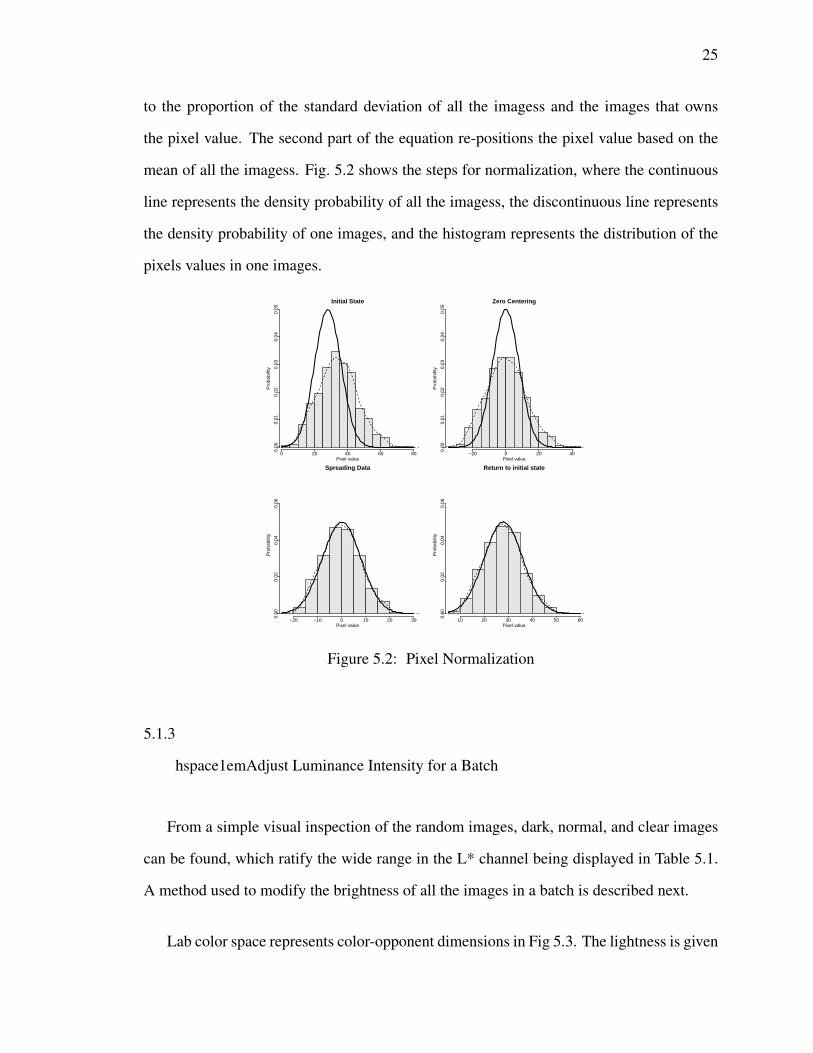
25
to the proportion of the standard deviation of all the imagess and the images that owns
the pixel value. The second part of the equation re-positions the pixel value based on the
mean of all the imagess. Fig. 5.2 shows the steps for normalization, where the continuous
line represents the density probability of all the imagess, the discontinuous line represents
the density probability of one images, and the histogram represents the distribution of the
pixels values in one images.
Initial State
samples
Den
sity
0 20 40 60 80
0.00
0.01
0.02
0.03
0.04
0.05
Pixel value
Pro
babi
lity
Zero Centering
samples
Den
sity
−20 0 20 40
0.00
0.01
0.02
0.03
0.04
0.05
Pixel value
Pro
babi
lity
Spreading Data
samples
Den
sity
−20 −10 0 10 20 30
0.00
0.02
0.04
0.06
Pixel value
Pro
babi
lity
Return to initial state
samples
Den
sity
10 20 30 40 50 60
0.00
0.02
0.04
0.06
Pixel value
Pro
babi
lity
Figure 5.2: Pixel Normalization
5.1.3
hspace1emAdjust Luminance Intensity for a Batch
From a simple visual inspection of the random images, dark, normal, and clear images
can be found, which ratify the wide range in the L* channel being displayed in Table 5.1.
A method used to modify the brightness of all the images in a batch is described next.
Lab color space represents color-opponent dimensions in Fig 5.3. The lightness is given
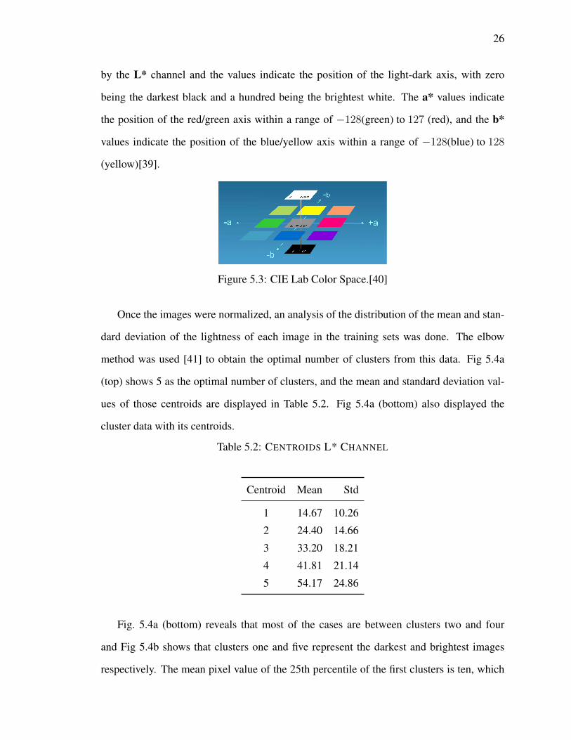
26
by the L* channel and the values indicate the position of the light-dark axis, with zero
being the darkest black and a hundred being the brightest white. The a* values indicate
the position of the red/green axis within a range of −128(green) to 127 (red), and the b*
values indicate the position of the blue/yellow axis within a range of −128(blue) to 128
(yellow)[39].
Figure 5.3: CIE Lab Color Space.[40]
Once the images were normalized, an analysis of the distribution of the mean and stan-
dard deviation of the lightness of each image in the training sets was done. The elbow
method was used [41] to obtain the optimal number of clusters from this data. Fig 5.4a
(top) shows 5 as the optimal number of clusters, and the mean and standard deviation val-
ues of those centroids are displayed in Table 5.2. Fig 5.4a (bottom) also displayed the
cluster data with its centroids.
Table 5.2: CENTROIDS L* CHANNEL
Centroid Mean Std
1 14.67 10.26
2 24.40 14.66
3 33.20 18.21
4 41.81 21.14
5 54.17 24.86
Fig. 5.4a (bottom) reveals that most of the cases are between clusters two and four
and Fig 5.4b shows that clusters one and five represent the darkest and brightest images
respectively. The mean pixel value of the 25th percentile of the first clusters is ten, which
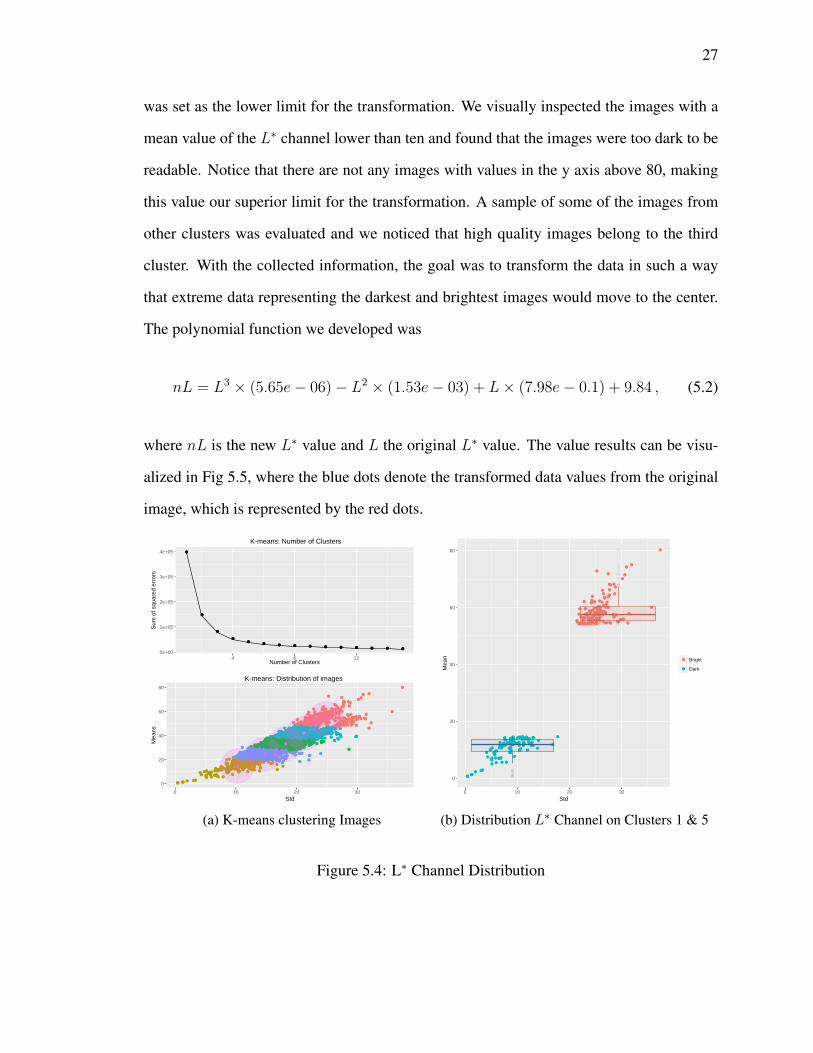
27
was set as the lower limit for the transformation. We visually inspected the images with a
mean value of the L∗ channel lower than ten and found that the images were too dark to be
readable. Notice that there are not any images with values in the y axis above 80, making
this value our superior limit for the transformation. A sample of some of the images from
other clusters was evaluated and we noticed that high quality images belong to the third
cluster. With the collected information, the goal was to transform the data in such a way
that extreme data representing the darkest and brightest images would move to the center.
The polynomial function we developed was
nL = L3 × (5.65e− 06)− L2 × (1.53e− 03) + L× (7.98e− 0.1) + 9.84 , (5.2)
where nL is the new L∗ value and L the original L∗ value. The value results can be visu-
alized in Fig 5.5, where the blue dots denote the transformed data values from the original
image, which is represented by the red dots.
●
●
●
●●
● ● ● ● ● ● ● ● ● ●
0e+00
1e+05
2e+05
3e+05
4e+05
4 8 12Number of Clusters
Sum
of s
quar
ed e
rror
s
K-means: Number of Clusters
● ●● ●
●
●
●●
●●
●
●
●
●●
●
●
●
●
●
●
●
●
●●
●
●
●
●●
●●
●
●
●●
●●
●
●
●
●
●
●●●
●
●
●
● ●●
●
●
●
●
● ●●
●●
●
●
●
●
●
●
●
●
●
●
●
●●
●
●
● ●
●
●●
●
● ●
●
●●
●
●
●●
●
●
●
●
●
●
●
●
●
●●
●
●
●
●
●
●●
●
●●
●●●
●
●
●
●●
●
●
●●
●
●
●
●
●
●
●
●●
●
●
● ●
● ●●●
●
●
●
●●●
●●
● ●
●
●
●
●
●
●●
●
●
●
●
●●
●
●
●
●
●
●
●
●
●
●●
●
●
●
●●●●
●
●
●
●
●
●
●
●●
● ●●
●
●●
●●
●
●●
●●
●
●
●
● ●
●
●●
● ●
●
●
●
●
●
●●●
●
●
●
●
●
●●
●
●
●
●
●
●
●
●●
●
●
●●
●●
●
●
●
●●
●
●
●● ●
●●
●
●●
●
●●
●
●
●
●
●
●
●
●●
●
●
●
●
●
●
●
●●
●●
●●●
●
●●
●
●●
●
●
●
●
●
●●
●
●
●
●
●●
●●
●●
●
●
●
●
●●
●
●
●
●
●
●
●●
●●
●●
●
●
●
● ●
●
●
●
●
●
●
●●
●
●●
●
●
●
●●
●
●
●
●
●
●
●
●
●
●
●●
●
●
●●
●
●
●●
●●
●●
●
●
●●
●●
●
●●
●●
●
●
●●
●
●
●
●
●
●
●
●●
●
●●
●●●
●●
●
●
●●
●
●
● ●
●●
●
●●
●
●
●
●
●
●
● ●●
●●
●
●● ●
●
●
●
●
●
●
●
●
●
●
●
●●
●
●●
●
●
●●
●
●
●●
●
●
●
●
●
●●
●
●
●●
●●
●
●
●
●
●
●
●
●●
● ●
●
●●
●
●
●
●
●
●
●
●●
●
●
●
●
●
●
●●
●●
●●
●
●
●
●●●
●
●
●
●
●
●
●
●
●
●●
●●
●
● ●
●●
●
●
●
●
●●●
● ●
● ●
●
●
●
●●
●●
●
●
●
●
●
●
●
●
● ●
●
●
●●
●
●
●
●●
●
●
●
●●
●
●
●
●
●
● ●
●
●
●
●
●●
●
●●
●
●
●
●
●●
●●
●
●
●
●
●
●
●
●
●
●
●
●
●
●
●
●
●
●
●
●
●
●
●
●
●●●
●
●
●●
●●
●
●
●
●
●
●
●
●
●
●●
●
●
●
●
●●
●
●
●
●
●●
●
●
●●
●
●
●
●
● ●●
●
●●
●
●●●●
●
●
●
●
●
● ●
●
● ●
●
●●●
●
●
●
●
●
●
● ●
●
●
●
●●
●
●
●
●
●
●●
● ●
●
●
●
●●
●
●
●
●
●●
●
●
●
●
●●
●
●
●
●
●
●
●●
●
●
●
●●
● ●
●
●
●●
●
●
●● ●●
●
●
●●
●
●●
●
●
●
●
●
●
●
●
●●
●
●
●
●
●
●
●
●
●
●●
●●●
●
●
●
●●
●
●
●
●
●
●
●●●
●
●
●
●
●
●
●
●
●
●●
●
●●
●
●
●
●
●
●
●
●●
●
●
●●
●
●
●
●
●●
●
●
● ●
●●
●
●●
●
●
●
●
●
●
●●
●
●
●
●
●
●
●
●
●
● ●
●
●
●
●
●●
●
●
●
●
●
●●
●
●
●
●
●
●
●
●
●
●
●
●
●
●
●
●
●
●
●
●
●
●
●
●●
●
●
●
●
●
●
●
●
●
● ●
●●
●
●
●
●
●
●
●
●
●
●
●
●
●●
●● ●
●
●
●●
●
●
●
●●
●
●●
●
●●
●
●●
●
●
●
●●
●●
●
●
●
●
●
●●
● ●
●
●
●
●
●●
●
●
●
●
●
●
●
●
●
●
● ●●
●●
●
●
●
●●
●
●
●
●
●
●
●
●●
●
●
●
●
●
●
●
●
●●
●●
●●
●●
●●
●
●
●
●●●
●
●
●
●
●
●
●
●
●●
●
●
●
●
●
●
●
●
●●
●
●
●
●
●●
●
● ●
●
●●
● ●
●
● ●●●
●●
●
●
●
●
●●
●
●
●
●
●
●
●
●
●
●
●●
● ●
●
●●
●
●
●
●●
●●
●
●
●
●
●
●
●
●
●
●
●●
●
●●
●
●●
●●
● ●
●
●
●
●
●●
●
●
●
●
●
●●
●
●
●
●
●
●●●●
●
●
●
●
●●
●●
●●
●●
●
●
●●
●
●
●
●
●
●
●●
●●
●
●
●●
●
●
●
●
●
●
●
●●
●
●●
●
● ●
●
●● ●
●
●
● ●
●●
●
●
●
●
●
●
●
●
●
●●●
●
●
●
●
● ●
●
●
●
●
●●
●
●
●
●
●
●
● ●
●
●
●●
●●
●●
●
●●
●
●
●
●
●●
●
●
●●
●●
●
●
●
●
●●●
●
●●
●
●
●
●
●● ●
●
●
●
●
●
●
●
●
●
●
●●
● ●
●●
●
●●
●
●
●●●
●
●
●
●
●
●
●
●
●
●
●
●
●
●
●●
●
●
●●
●
●
●
●
●●
●
●●●
●
●
●
●●
●
●
●●
●●●●
●
●
●
●
●
●
●
●
●●
●
●
●●
●
●
●
●
●
●
●
●
●
●
●
●●
●
●
●
●
●●
●
●
●
●●
●●
●
●
●
●
●
●
●
●
● ●
●
●
●
●
● ●
●
●
●
●●
●
●
●
●
●
●●●●
●
●
●●●
●●
●
●
●●
●●
●
●
●
●
●
●
●
●
●
●
●●
●
●
●
●
●●
●
●
●
●
●●
●
●
●
●
●
●
●
● ●
●
●●
●
●
●
●
●
● ●
●●
●
●●
●●
●●
●
●●●
●
●
●
●
●●
●
●
●
●
●
●●
●
●
●
●●
●
●●
●
●
●
●
●
●
●
●
●
●
●
●
●
●
●
●●
●
●
●
●●
●
●
●
●
●●
●
●
●
●
●
●
●
●
●
●
●
●
●
●●
●●
●
●●
●
●
●
●
●
●●
●
●
● ●
●●
●
●
●
●
●
●
●
●
●
●
●
●
●
● ●
●
●
●
●● ●
●
●
●●
●●
●
●●
●
● ●
●
●
●
●●
●●
●
●
●
●
●
●
●●
●
●●
●
●
●
●
●
●
●
●●●
●
●
●
●
●
●
●
●●
●
●
●●●
●●
●
●
●
●
●●●
●
●
●
●
●
●
●
●
●●
●
●●
●
● ●
●
●
●
●
●
●●
●●
●●
●●
●
●●
●
●
● ●
●
●●
●
●
● ●
●
●
●●●
●
●
● ●
●
●
● ●
●
●
●
●
●●
●●
●
●
●
●
●
●
●
●
●
●
●●
●
●
●
● ●
●
●
●
●
●
●
●
●
●
●●
●
●
●
●
●
●
●● ●● ●●●
●
●
●●
●
●
●
●
●
●
●●
●
●
●
●
●
●
●●
●
●
●
●
●
●
●
●
●
●
●
●
●
●
●
●●
●
●
●
●
●●
●
●
●
●
●●●
●
●
●
●
●●
●
●
●●
●
●
●●
●
●
●
●
●
●
●
●
●
●
●
●
●
●
●
●
●
●
●
●
●
●
●● ●
●●
●
●
●
●
●
●
●
●
● ●
●
●
●●
●
●●
●
●●
●●
●●
●
●●
●●
●
●●
●
●●
●
●
●
●
●●●
●●
●
●
●●
●●
●
●●
●
● ●
●
●●●●
●
●
●
●
●
●● ●
●
●●
●●
●
●
●
●
●
●
●
● ●
● ●
●●
●
●
●
●
●
● ●
●●●
●
●
●
●●
●●
●
●●
● ●●
●●
●
●
●
● ●
● ●
●
●●
●
●
●
●●
●
● ●
●
●
●
●
●
●●
● ●
●
●
●
●
●
●●●
●
●
●
●
● ●
●
●
●
●●
●
●
●●
●
●
●
●
●
●
●
●
●●
●●
●
●
●
●
●
●
●
●
●
●
●
● ●
●
●
●
●
●
●
●
●
●●
●
●
●
●
● ●
●
●
●
●●
●
●
●
●
●
●
●
●
●
●
●
●
●
●● ●
●●
●
●
●
●
● ●
●
●
●
●
●●
●
●
● ●
●
●
●●
●
●
●
●
●
●
●
●
●
●
●
●
●
●
●
●●
●
●
● ●
● ●
●●●●
●
●●
●●
●
●
●●
●●
●●
●●
●
●
●
●
●
●
●
●
●
●
●●
●
●
●
●
●
●●
●●●
●
●●
●
●●
●●
●
● ●
●
●
●●●
●●
●
●●
●
●
●
●
●
●
●
●
● ●
●●
●●
●●
●
●
●
●
●
● ●
●
●
●
●
●●
●
●
●●
●
●
●
●
●
●
●
●●●
●
●●
●
●
●
●
●●
●
●
●●
●
●
●●
● ●
●
●
●●
●
●
● ●
●
●
●
●
●●
●●
●
●
●
●●
●
●●
●
●●
● ●
●
●●
●
●●
●●
●
●
●
●
●●
●
●
●
●●
●
●●
●
●
●
●
●
● ●
●
●●
●
●
●
●
●
●
●
●
●●● ●
●
●
●
●●●
●
●
● ●
●
●
●
●
●
●
●●
●
●
●
●●
●
●
●●
●
●
●
●
●
●
●
●
●
● ●●
●
●
●
●
●
●
●
●
●
●●
●●●
●
●
●
●
●
●
●
●
●
●
●
●
●
●
●
●
●●●
● ●
●
●
●
●
●●
●
● ●●
●●
●●
●
●
●
●
●
●
●●
●
●●
●●
●
●
●
●
●
●
●
●
●
●
●
●
●
●
●
●
●
●
●
●
●
● ●
●
●
●
●
●
●
●
●●
●
●
●●
●
●
●
●● ●
●
●●
●
●
●●
●
●
●
●
●
●
●
●
●
0
20
40
60
80
0 10 20 30
Std
Mea
ns
K-means: Distribution of images
(a) K-means clustering Images
●
●●●
●
●●
●
●
●
●
●
●●
●
●●
●
●
●
●
●
●
●
●
●
●
●●
●
●
●
●●
●
●● ● ●●
●
● ●
●
●
●
●
●
●
●
●
●
●●
●
●
●
●●
●
●
●●
● ●
●●
●
●
●
●
●●
●●
●
●●
●
●
●
●
●
●●
●
●
●
●
●●
●● ●
●
●
●
●●●
●
●
●
●
● ●
●
●
●
●●
●
●
●
●
●●●
●
●
●
●●
●
●
●
●
●
●
●
●●
●
●
●
●●
●
●
●
●
●
●
●
●
●
● ●●
●
●
●●
●
●
●
●
●●
●●
●
●
●●
●
●
●●●
●
●
●
●
●
●
●●
●
●
● ●●
●●
●●
●
●
●●
● ●
●
●
●
●
●●
●● ●
●
●
●
● ●
●
●●
●●
●
●
● ●
●
●
●
●
●
●
●●
●
●
●
●●
●●
●
●●
0
20
40
60
80
0 10 20 30
Std
Mea
n
●
●
Bright
Dark
(b) Distribution L∗ Channel on Clusters 1 & 5
Figure 5.4: L∗ Channel Distribution

28
Figure 5.5: Distribution L* Channel on Clusters 1 & 5 Before and After Transformation
5.1.4
hspace1emReducing Color Variance
Just like any blood extravasation, the microaneurysm color goes through a sequence of
changes, the most common sequence going from a bright red, to a brownish, to a yellowish
color. Because our purpose was to enhance microaneurysms, we limited the scene in order
to separate blood tissues from other structures using a novel approach.
After the normalization and the adjustment of the L∗ values, we built a dataset with
pixel values from vessels including microaneurysms and other structures like the optical
disk, macula, exudates, and normal retina among others. Table 5.3 shows a wide range for
a∗ and b∗ values and a difference in the vessels and background groups mean. In Fig. 5.6a
each point represents the a* and b* pixels’ values of the vessels and background pixels. In
addition, there is a blue line separating the two groups that were obtained using the Linear
Support Vector Machine, and two black points that are equidistant and orthogonal to the
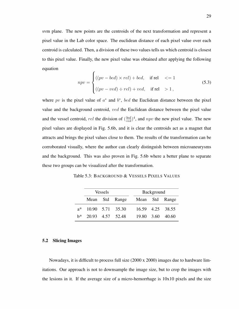
29
svm plane. The new points are the centroids of the next transformation and represent a
pixel value in the Lab color space. The euclidean distance of each pixel value over each
centroid is calculated. Then, a division of these two values tells us which centroid is closest
to this pixel value. Finally, the new pixel value was obtained after applying the following
equation
npv =
((pv − bed)× rel) + bed, if rel <= 1
((pv − ved)÷ rel) + ved, if rel > 1 ,
(5.3)
where pv is the pixel value of a∗ and b∗, bed the Euclidean distance between the pixel
value and the background centroid, ved the Euclidean distance between the pixel value
and the vessel centroid, rel the division of ( bedved
)4, and npv the new pixel value. The new
pixel values are displayed in Fig. 5.6b, and it is clear the centroids act as a magnet that
attracts and brings the pixel values close to them. The results of the transformation can be
corroborated visually, where the author can clearly distinguish between microaneurysms
and the background. This was also proven in Fig. 5.6b where a better plane to separate
these two groups can be visualized after the transformation.
Table 5.3: BACKGROUND & VESSELS PIXELS VALUES
Vessels Background
Mean Std Range Mean Std Range
a* 10.90 5.71 35.30 16.59 4.25 38.55
b* 20.93 4.57 52.48 19.80 3.60 40.60
5.2 Slicing Images
Nowadays, it is difficult to process full size (2000 x 2000) images due to hardware lim-
itations. Our approach is not to downsample the image size, but to crop the images with
the lesions in it. If the average size of a micro-hemorrhage is 10x10 pixels and the size
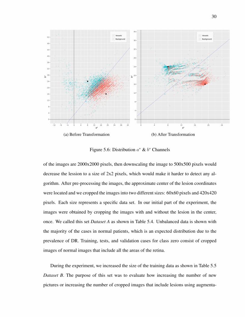
30
●
●
0
4
8
12
16
20
24
28
32
36
40
44
48
52
−12 −8 −4 0 4 8 12 16 20 24 28 32 36 40
a*
b*
Vessels
Background
(a) Before Transformation
●
●
0
4
8
12
16
20
24
28
32
36
40
0 4 8 12 16 20 24
a*
b*
Vessels
Background
(b) After Transformation
Figure 5.6: Distribution a∗ & b∗ Channels
of the images are 2000x2000 pixels, then downscaling the image to 500x500 pixels would
decrease the lession to a size of 2x2 pixels, which would make it harder to detect any al-
gorithm. After pre-processing the images, the approximate center of the lesion coordinates
were located and we cropped the images into two different sizes: 60x60 pixels and 420x420
pixels. Each size represents a specific data set. In our initial part of the experiment, the
images were obtained by cropping the images with and without the lesion in the center,
once. We called this set Dataset A as shown in Table 5.4. Unbalanced data is shown with
the majority of the cases in normal patients, which is an expected distribution due to the
prevalence of DR. Training, tests, and validation cases for class zero consist of cropped
images of normal images that include all the areas of the retina.
During the experiment, we increased the size of the training data as shown in Table 5.5
Dataset B. The purpose of this set was to evaluate how increasing the number of new
pictures or increasing the number of cropped images that include lesions using augmenta-
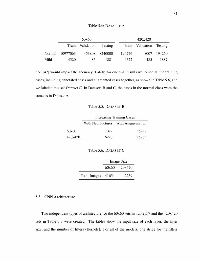
31
Table 5.4: DATASET A
60x60 420x420
Train Validation Testing Train Validation Testing
Normal 10977063 453808 8240000 194276 8007 194260
Mild 4520 485 1881 4522 485 1887
tion [42] would impact the accuracy. Lately, for our final results we joined all the training
cases, including annotated cases and augmented cases together, as shown in Table 5.6, and
we labeled this set Dataset C. In Datasets B and C, the cases in the normal class were the
same as in Dataset A.
Table 5.5: DATASET B
Increasing Training Cases
With New Pictures With Augmentation
60x60 7072 15798
420x420 6990 15765
Table 5.6: DATASET C
Image Size
60x60 420x420
Total Images 41654 42259
5.3 CNN Architecture
Two independent types of architecture for the 60x60 sets in Table 5.7 and the 420x420
sets in Table 5.8 were created. The tables show the input size of each layer, the filter
size, and the number of filters (Kernels). For all of the models, one stride for the filters
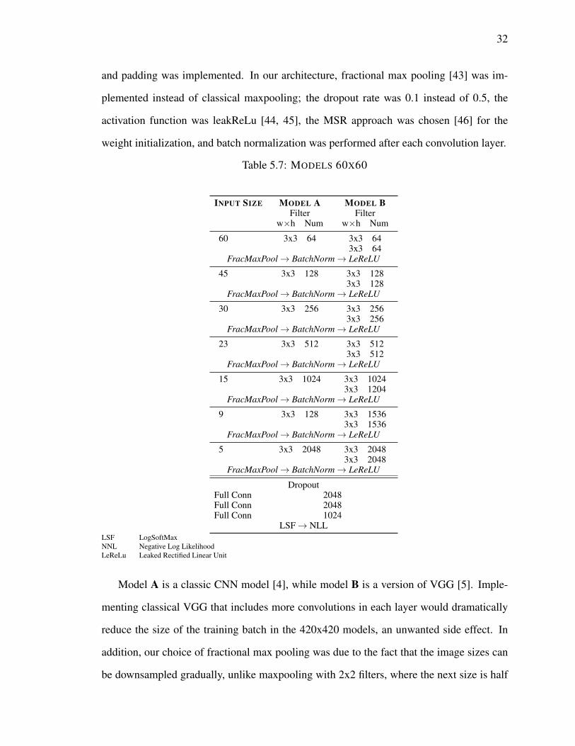
32
and padding was implemented. In our architecture, fractional max pooling [43] was im-
plemented instead of classical maxpooling; the dropout rate was 0.1 instead of 0.5, the
activation function was leakReLu [44, 45], the MSR approach was chosen [46] for the
weight initialization, and batch normalization was performed after each convolution layer.
Table 5.7: MODELS 60X60
INPUT SIZE MODEL A MODEL BFilter Filter
w×h Num w×h Num
60 3x3 64 3x3 643x3 64
FracMaxPool→ BatchNorm→ LeReLU
45 3x3 128 3x3 1283x3 128
FracMaxPool→ BatchNorm→ LeReLU
30 3x3 256 3x3 2563x3 256
FracMaxPool→ BatchNorm→ LeReLU
23 3x3 512 3x3 5123x3 512
FracMaxPool→ BatchNorm→ LeReLU
15 3x3 1024 3x3 10243x3 1204
FracMaxPool→ BatchNorm→ LeReLU
9 3x3 128 3x3 15363x3 1536
FracMaxPool→ BatchNorm→ LeReLU
5 3x3 2048 3x3 20483x3 2048
FracMaxPool→ BatchNorm→ LeReLU
DropoutFull Conn 2048Full Conn 2048Full Conn 1024
LSF→ NLLLSF LogSoftMaxNNL Negative Log LikelihoodLeReLu Leaked Rectified Linear Unit
Model A is a classic CNN model [4], while model B is a version of VGG [5]. Imple-
menting classical VGG that includes more convolutions in each layer would dramatically
reduce the size of the training batch in the 420x420 models, an unwanted side effect. In
addition, our choice of fractional max pooling was due to the fact that the image sizes can
be downsampled gradually, unlike maxpooling with 2x2 filters, where the next size is half

33
of the previous one.
For the classification phase, a variation of increasing the number of dropout layers and
the rate of probability was implemented in model B as shown in Table 5.9. Furthermore,
the performance of this model is compared with other models.
5.4 Feedback
The torch script applied to our experiments randomly chose between using a normal
or mild DR class for the next input. After the group was selected, the script, once again,
randomly chose a picture from the data pool of the class, making the processes completely
stochastic. In addition, a feedback mechanism was created during training, in order to
resend the images that were not classified correctly.
The difference of the values between the current loss function and that of the prior batch
greater than zero indicates that the current batch did not classify as well as the previous
batch. This is the basis of our feedback function. The function created for the feedback
detects the batch in which the current difference of the values of the cost function surpass
the moving average of the mean of the differences of the previous batches. The polynomial
function used in our feedback is as follows:
cve = bn4 × (−1.41e− 20) + bn3 × (2.08e− 15) + bn2
×− (9.84e− 11) + bn× 6.27e− 07 + (1.50e− 01) ,
(5.4)
where bn is the batch number and cve the cost value expected. If the cost value of the batch
during the training was greater than we expected it to be after applying the equation 5.4,
we resent the same batch for re-training as shown in Fig. 5.7.
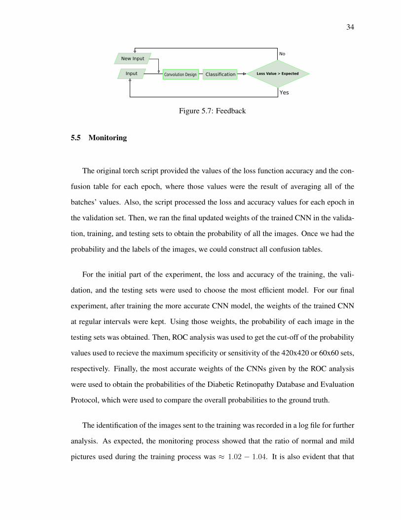
34
Input
No
Yes
Classification
New Input
Loss Value > ExpectedConvolution Design
Figure 5.7: Feedback
5.5 Monitoring
The original torch script provided the values of the loss function accuracy and the con-
fusion table for each epoch, where those values were the result of averaging all of the
batches’ values. Also, the script processed the loss and accuracy values for each epoch in
the validation set. Then, we ran the final updated weights of the trained CNN in the valida-
tion, training, and testing sets to obtain the probability of all the images. Once we had the
probability and the labels of the images, we could construct all confusion tables.
For the initial part of the experiment, the loss and accuracy of the training, the vali-
dation, and the testing sets were used to choose the most efficient model. For our final
experiment, after training the more accurate CNN model, the weights of the trained CNN
at regular intervals were kept. Using those weights, the probability of each image in the
testing sets was obtained. Then, ROC analysis was used to get the cut-off of the probability
values used to recieve the maximum specificity or sensitivity of the 420x420 or 60x60 sets,
respectively. Finally, the most accurate weights of the CNNs given by the ROC analysis
were used to obtain the probabilities of the Diabetic Retinopathy Database and Evaluation
Protocol, which were used to compare the overall probabilities to the ground truth.
The identification of the images sent to the training was recorded in a log file for further
analysis. As expected, the monitoring process showed that the ratio of normal and mild
pictures used during the training process was ≈ 1.02 − 1.04. It is also evident that that
35
the number of repeated images of the mild class was bigger than the number of repeated
images of the normal class due to their pool-size.
5.5.1
hspace1emROC
ROC [38] is a graphical representation of discriminatory tests over two populations
where the x-axis represents the sensitivity, the y-axis represents 1 − specificity, and the
curve shows all threshold values. Several indexes were developed to summarize ROC in
one value such as the area under ROC. Also, a method to find the optimal cut point, where
sensitivity and specificity are maximized, such as the Younden Index was used in this study.
Youndex Index is the minimimun Euclidean distance of the top left corner, where sensitivity
and specificity are equal to one, and the ROC curve. The package OptimalCutpoints 1, from
Rcran was used to obtain the optimal points of the max sensitivity and specificity.
1https://cran.r-project.org/web/packages/OptimalCutpoints/index.html
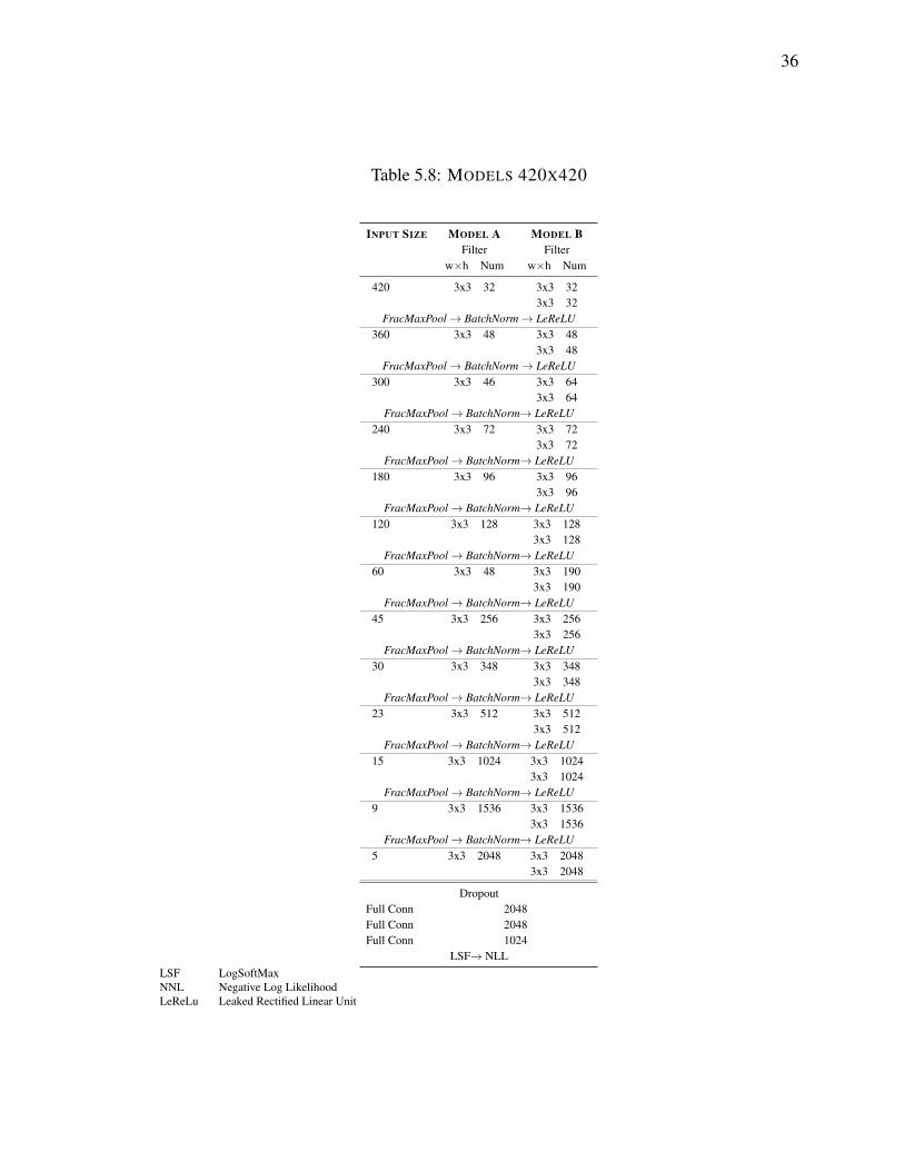
36
Table 5.8: MODELS 420X420
INPUT SIZE MODEL A MODEL BFilter Filter
w×h Num w×h Num
420 3x3 32 3x3 323x3 32
FracMaxPool→ BatchNorm→ LeReLU360 3x3 48 3x3 48
3x3 48FracMaxPool→ BatchNorm→ LeReLU
300 3x3 46 3x3 643x3 64
FracMaxPool→ BatchNorm→ LeReLU240 3x3 72 3x3 72
3x3 72FracMaxPool→ BatchNorm→ LeReLU
180 3x3 96 3x3 963x3 96
FracMaxPool→ BatchNorm→ LeReLU120 3x3 128 3x3 128
3x3 128FracMaxPool→ BatchNorm→ LeReLU
60 3x3 48 3x3 1903x3 190
FracMaxPool→ BatchNorm→ LeReLU45 3x3 256 3x3 256
3x3 256FracMaxPool→ BatchNorm→ LeReLU
30 3x3 348 3x3 3483x3 348
FracMaxPool→ BatchNorm→ LeReLU23 3x3 512 3x3 512
3x3 512FracMaxPool→ BatchNorm→ LeReLU
15 3x3 1024 3x3 10243x3 1024
FracMaxPool→ BatchNorm→ LeReLU9 3x3 1536 3x3 1536
3x3 1536FracMaxPool→ BatchNorm→ LeReLU
5 3x3 2048 3x3 20483x3 2048
DropoutFull Conn 2048Full Conn 2048Full Conn 1024
LSF→ NLLLSF LogSoftMaxNNL Negative Log LikelihoodLeReLu Leaked Rectified Linear Unit

37
Table 5.9: DROPOUT SETTING
Dropout 0.5
Full Conn 2048
Dropout 0.5
Full Conn 2048
Dropout 0.5
Full Conn 1024
LSF→ NNL

38
CHAPTER 6
EXPERIMENTAL DESIGN AND RESULTS
For this study, we divided the CNN in 4 phases. The first phase is the input-phase,
where input processing used to enhance features and augmentation of the dataset is per-
formed. The second phase is the Convolution Design-phase, where modifications to the
number of convolutions and filters can be completed. Variation of the type of pooling, nor-
malization,and neural activation function is also possible in this stage. The classification-
phase or the third phase, includes full-connected layers with the neural activation function
and loss function. The dropout of nodes in a full-connected layer in this phase has been
a common modification, in recent studies. The fourth phase is the training-phase, where
we can alter the hyper-parameters, learning algorithms, and perform feedback. Following
pedantic rules, each phase should be evaluated separately, in order to measure the impact
of changing a parameter on that phase, though changing only a parameter at any point is
often unpractical.
Our plan for the study was to select the modifications in the input, convolution design,
classification, and training phase that would improve our sensitivity and specificity in the
training, validation, and testing sets. Dataset C was trained with all the previous modifi-
cations, in order to get the weights that performed best in the testing sets and the cutoff
point values provided by ROC analysis to achieve the optimal sensitivity and specificity.
Finally, the Diabetic Retinopathy Database and Evaluation Protocol dataset was tested and
the results were compared to their own groundtruth.
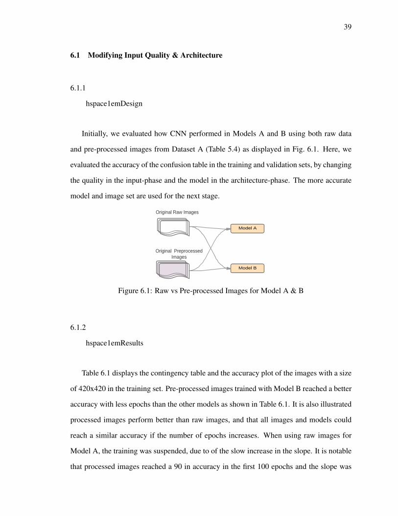
39
6.1 Modifying Input Quality & Architecture
6.1.1
hspace1emDesign
Initially, we evaluated how CNN performed in Models A and B using both raw data
and pre-processed images from Dataset A (Table 5.4) as displayed in Fig. 6.1. Here, we
evaluated the accuracy of the confusion table in the training and validation sets, by changing
the quality in the input-phase and the model in the architecture-phase. The more accurate
model and image set are used for the next stage.
Figure 6.1: Raw vs Pre-processed Images for Model A & B
6.1.2
hspace1emResults
Table 6.1 displays the contingency table and the accuracy plot of the images with a size
of 420x420 in the training set. Pre-processed images trained with Model B reached a better
accuracy with less epochs than the other models as shown in Table 6.1. It is also illustrated
processed images perform better than raw images, and that all images and models could
reach a similar accuracy if the number of epochs increases. When using raw images for
Model A, the training was suspended, due to of the slow increase in the slope. It is notable
that processed images reached a 90 in accuracy in the first 100 epochs and the slope was
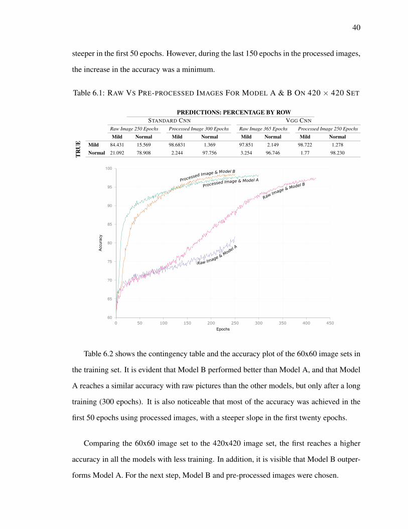
40
steeper in the first 50 epochs. However, during the last 150 epochs in the processed images,
the increase in the accuracy was a minimum.
Table 6.1: RAW VS PRE-PROCESSED IMAGES FOR MODEL A & B ON 420 × 420 SET
PREDICTIONS: PERCENTAGE BY ROWSTANDARD CNN VGG CNN
Raw Image 250 Epochs Processed Image 300 Epochs Raw Image 365 Epochs Processed Image 250 Epochs
Mild Normal Mild Normal Mild Normal Mild Normal
TR
UE Mild 84.431 15.569 98.6831 1.369 97.851 2.149 98.722 1.278
Normal 21.092 78.908 2.244 97.756 3.254 96.746 1.77 98.230
60
65
70
75
80
85
90
95
100
0 50 100 150 200 250 300 350 400 450
Accu
racy
Epochs
Processed Image & Model B
Processed Image & Model A
Raw Image & Model B
Raw Image & Model A
Table 6.2 shows the contingency table and the accuracy plot of the 60x60 image sets in
the training set. It is evident that Model B performed better than Model A, and that Model
A reaches a similar accuracy with raw pictures than the other models, but only after a long
training (300 epochs). It is also noticeable that most of the accuracy was achieved in the
first 50 epochs using processed images, with a steeper slope in the first twenty epochs.
Comparing the 60x60 image set to the 420x420 image set, the first reaches a higher
accuracy in all the models with less training. In addition, it is visible that Model B outper-
forms Model A. For the next step, Model B and pre-processed images were chosen.
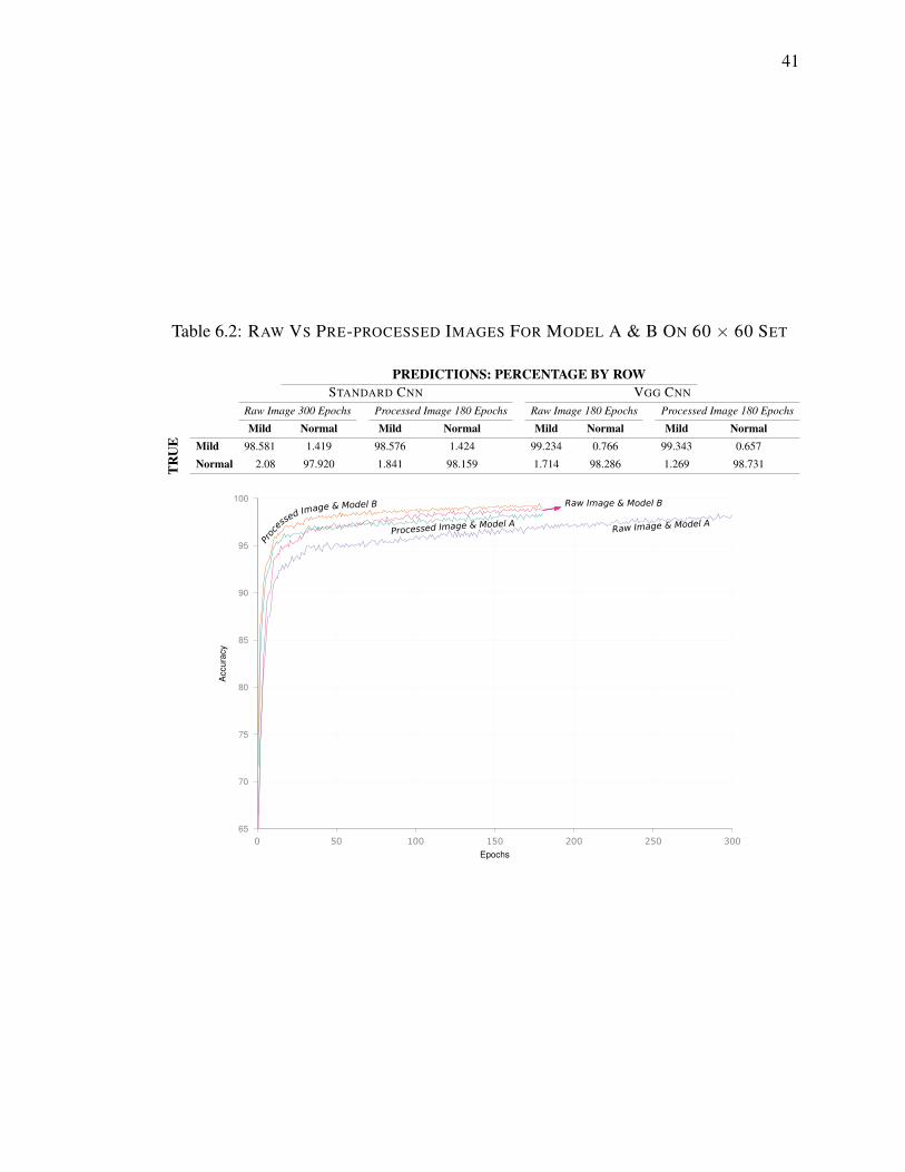
41
Table 6.2: RAW VS PRE-PROCESSED IMAGES FOR MODEL A & B ON 60 × 60 SET
PREDICTIONS: PERCENTAGE BY ROWSTANDARD CNN VGG CNN
Raw Image 300 Epochs Processed Image 180 Epochs Raw Image 180 Epochs Processed Image 180 Epochs
Mild Normal Mild Normal Mild Normal Mild Normal
TR
UE Mild 98.581 1.419 98.576 1.424 99.234 0.766 99.343 0.657
Normal 2.08 97.920 1.841 98.159 1.714 98.286 1.269 98.731
65
70
75
80
85
90
95
100
0 50 100 150 200 250 300
Accu
racy
Epochs
Proc
essed Image & Model B
Processed Image & Model ARaw Image & Model A
Raw Image & Model B
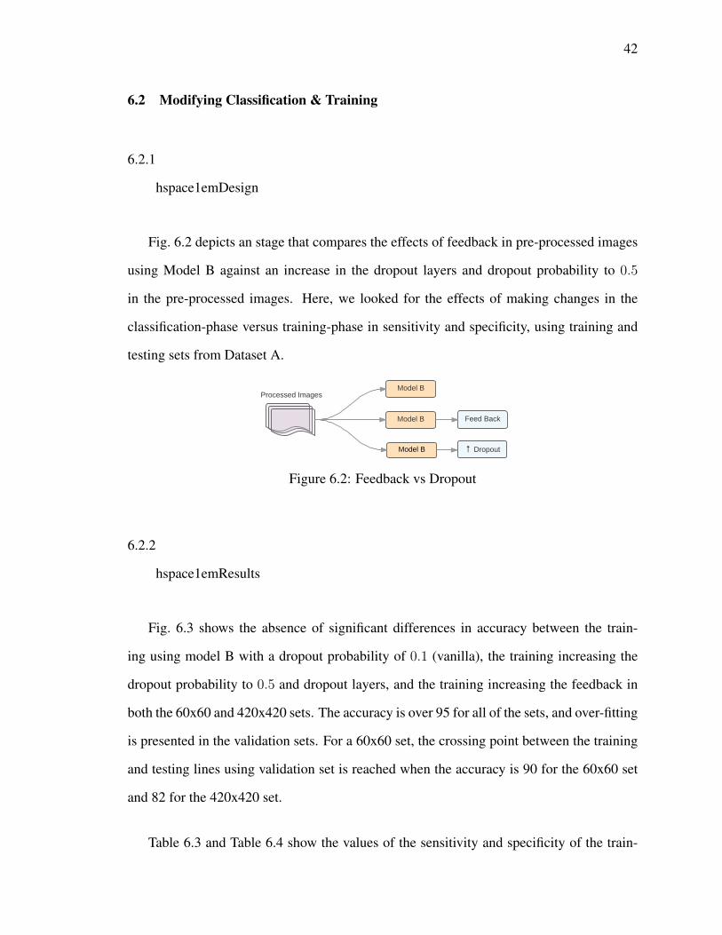
42
6.2 Modifying Classification & Training
6.2.1
hspace1emDesign
Fig. 6.2 depicts an stage that compares the effects of feedback in pre-processed images
using Model B against an increase in the dropout layers and dropout probability to 0.5
in the pre-processed images. Here, we looked for the effects of making changes in the
classification-phase versus training-phase in sensitivity and specificity, using training and
testing sets from Dataset A.
Figure 6.2: Feedback vs Dropout
6.2.2
hspace1emResults
Fig. 6.3 shows the absence of significant differences in accuracy between the train-
ing using model B with a dropout probability of 0.1 (vanilla), the training increasing the
dropout probability to 0.5 and dropout layers, and the training increasing the feedback in
both the 60x60 and 420x420 sets. The accuracy is over 95 for all of the sets, and over-fitting
is presented in the validation sets. For a 60x60 set, the crossing point between the training
and testing lines using validation set is reached when the accuracy is 90 for the 60x60 set
and 82 for the 420x420 set.
Table 6.3 and Table 6.4 show the values of the sensitivity and specificity of the train-
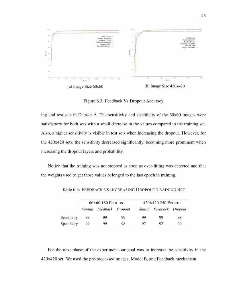
43
60
65
70
75
80
85
90
95
100
0 20 40 60 80 100 120 140 160 180
Acc
urac
y
Epochs
Vanilla TrainVanilla Validation
Feedback TrainFeedback Validation
Dropout TrainDropout Validation
(a) Image Size 60x60
30
40
50
60
70
80
90
100
0 50 100 150 200 250
Acc
urac
y
Epochs
Vanilla TrainVanilla Validation
Feedback TrainFeedback Validation
Dropout TrainDropout Validation
(b) Image Size 420x420
Figure 6.3: Feedback Vs Dropout Accuracy
ing and test sets in Dataset A. The sensitivity and specificity of the 60x60 images were
satisfactory for both sets with a small decrease in the values compared to the training set.
Also, a higher sensitivity is visible in test sets when increasing the dropout. However, for
the 420x420 sets, the sensitivity decreased significantly, becoming more prominent when
increasing the dropout layers and probability.
Notice that the training was not stopped as soon as over-fitting was detected and that
the weights used to get those values belonged to the last epoch in training.
Table 6.3: FEEDBACK VS INCREASING DROPOUT TRAINING SET
60X60 180 EPOCHS 420X420 250 EPOCHS
Vanilla Feedback Dropout Vanilla Feedback Dropout
Sensitivity 99 99 99 99 99 98
Specificity 99 99 98 97 97 99
For the next phase of the experiment our goal was to increase the sensitivity in the
420x420 set. We used the pre-processed images, Model B, and Feedback mechanism.

44
Table 6.4: FEEBACK VS INVREASING DROPOUT TESTING SET
60X60 180 EPOCHS 420X420 250 EPOCHS
Vanilla Feedback Dropout Vanilla Feedback Dropout
Sensitivity 92 92 96 62 67 61
Specificity 99 99 98 97 97 99
6.3 Modifying Input Quantity
6.3.1
hspace1emDesign
Fig 6.4 illustrates the design comparing the changes corresponding to increases in size
of input by using augmentation against increases in size of input by adding new images
to the dataset (Dataset B), where the previous stage performed better in the 420x420 set.
The performance is evaluated by measuring the sensitivity and specificity of the testing set
using different epochs.
Of the new cases provided by the Messidor dataset, 1276 were added to the 60x60
set and 1199 were added to the 420x420 set. Dataset B consists of the new cases and
cropped images with the lesion not centered. The augmentation set consists of images from
Dataset A and six cropped images with the lesion not centered assuring that the images are
completely different.
6.3.2
hspace1emResults
The accuracy plot of the training set in Fig. 6.5 shows that the input augmentation
reached a higher accuracy than the new input at the beginning of the training, but at the
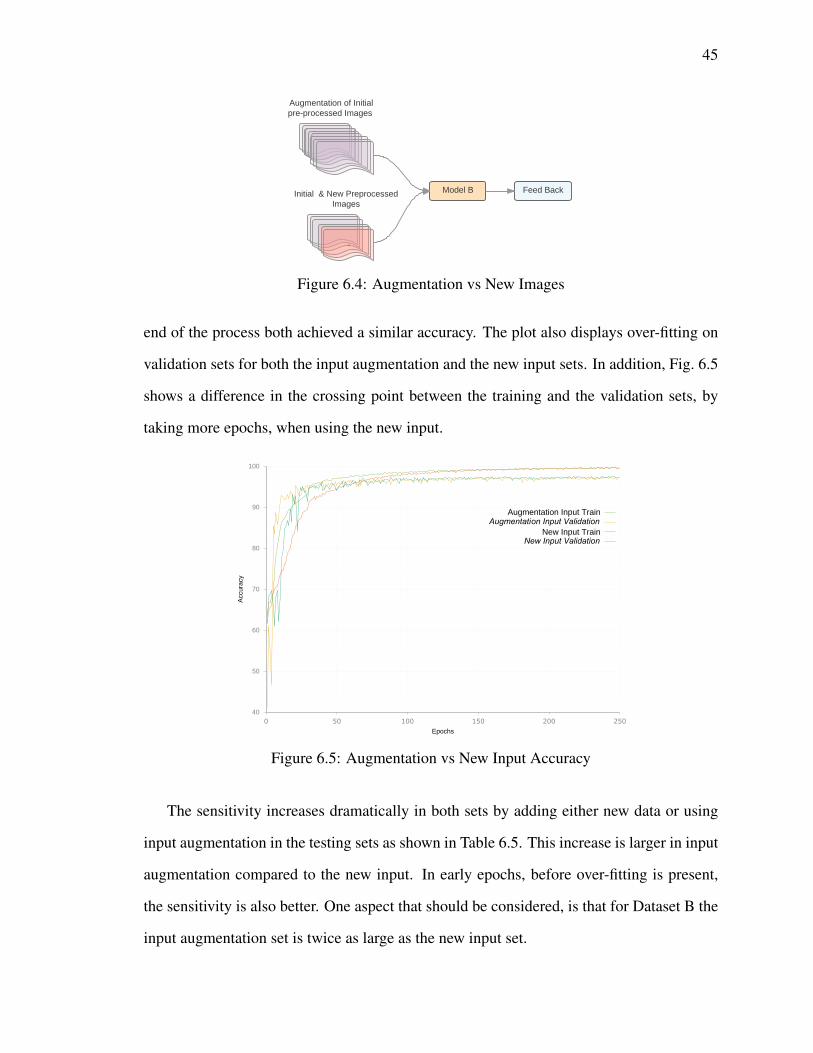
45
Figure 6.4: Augmentation vs New Images
end of the process both achieved a similar accuracy. The plot also displays over-fitting on
validation sets for both the input augmentation and the new input sets. In addition, Fig. 6.5
shows a difference in the crossing point between the training and the validation sets, by
taking more epochs, when using the new input.
40
50
60
70
80
90
100
0 50 100 150 200 250
Acc
urac
y
Epochs
Augmentation Input TrainAugmentation Input Validation
New Input TrainNew Input Validation
Figure 6.5: Augmentation vs New Input Accuracy
The sensitivity increases dramatically in both sets by adding either new data or using
input augmentation in the testing sets as shown in Table 6.5. This increase is larger in input
augmentation compared to the new input. In early epochs, before over-fitting is present,
the sensitivity is also better. One aspect that should be considered, is that for Dataset B the
input augmentation set is twice as large as the new input set.
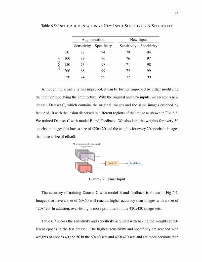
46
Table 6.5: INPUT AUGMENTATION VS NEW INPUT SENSITIVITY & SPECIFICITY
Augmentation New Input
Sensitivity Specificity Sensitivity Specificity
Epo
chs
50 82 94 79 94
100 79 96 76 97
150 73 98 71 98
200 68 99 72 99
250 74 99 72 99
Although the sensitivity has improved, it can be further improved by either modifying
the input or modifying the architecture. With the original and new inputs, we created a new
dataset, Dataset C, which contains the original images and the same images cropped by
factor of 10 with the lesion dispersed in different regions of the image as shown in Fig. 6.6.
We trained Dataset C with model B and Feedback. We also kept the weights for every 50
epochs in images that have a size of 420x420 and the weights for every 20 epochs in images
that have a size of 60x60.
Figure 6.6: Final Input
The accuracy of training Dataset C with model B and feedback is shown in Fig 6.7.
Images that have a size of 60x60 will reach a higher accuracy than images with a size of
420x420. In addition, over-fitting is more prominent in the 420x420 image sets.
Table 6.7 shows the sensitivity and specificity acquired with having the weights at dif-
ferent epochs in the test dataset. The highest sensitivity and specificity are reached with
weights of epochs 40 and 50 in the 60x60 sets and 420x420 sets and are more accurate than
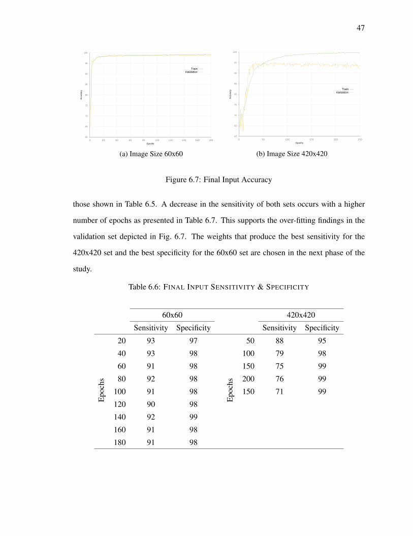
47
60
65
70
75
80
85
90
95
100
0 20 40 60 80 100 120 140 160 180
Acc
urac
y
Epochs
TrainValidation
(a) Image Size 60x60
60
65
70
75
80
85
90
95
100
0 50 100 150 200 250
Acc
urac
y
Epochs
TrainValidation
(b) Image Size 420x420
Figure 6.7: Final Input Accuracy
those shown in Table 6.5. A decrease in the sensitivity of both sets occurs with a higher
number of epochs as presented in Table 6.7. This supports the over-fitting findings in the
validation set depicted in Fig. 6.7. The weights that produce the best sensitivity for the
420x420 set and the best specificity for the 60x60 set are chosen in the next phase of the
study.
Table 6.6: FINAL INPUT SENSITIVITY & SPECIFICITY
60x60 420x420
Sensitivity Specificity Sensitivity Specificity
Epo
chs
20 93 97
Epo
chs
50 88 95
40 93 98 100 79 98
60 91 98 150 75 99
80 92 98 200 76 99
100 91 98 150 71 99
120 90 98
140 92 99
160 91 98
180 91 98
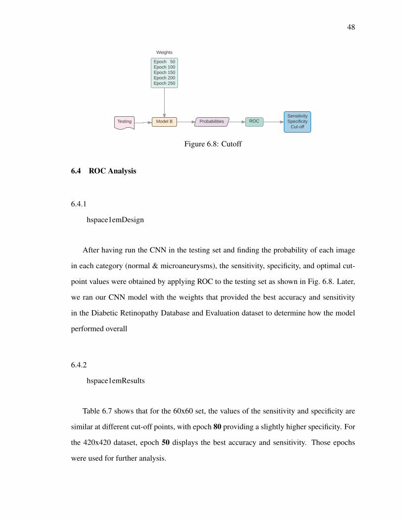
48
Figure 6.8: Cutoff
6.4 ROC Analysis
6.4.1
hspace1emDesign
After having run the CNN in the testing set and finding the probability of each image
in each category (normal & microaneurysms), the sensitivity, specificity, and optimal cut-
point values were obtained by applying ROC to the testing set as shown in Fig. 6.8. Later,
we ran our CNN model with the weights that provided the best accuracy and sensitivity
in the Diabetic Retinopathy Database and Evaluation dataset to determine how the model
performed overall
6.4.2
hspace1emResults
Table 6.7 shows that for the 60x60 set, the values of the sensitivity and specificity are
similar at different cut-off points, with epoch 80 providing a slightly higher specificity. For
the 420x420 dataset, epoch 50 displays the best accuracy and sensitivity. Those epochs
were used for further analysis.
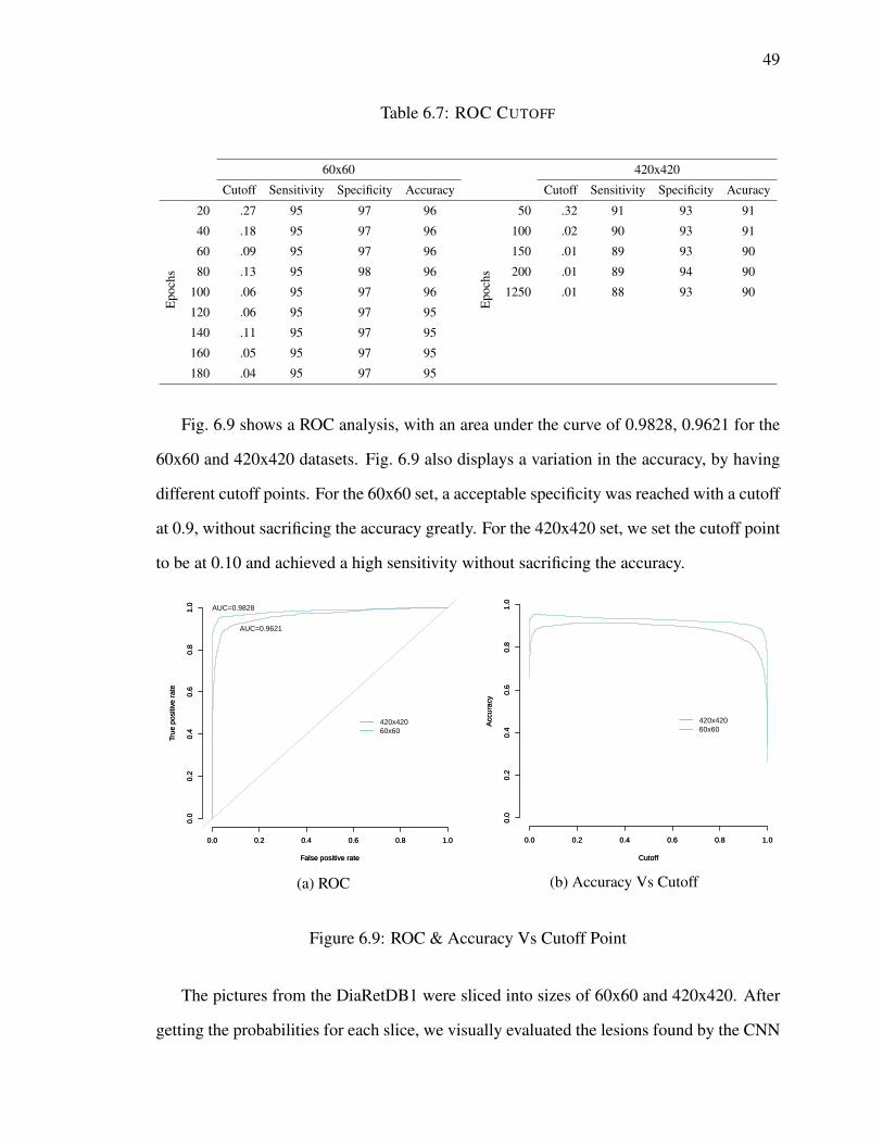
49
Table 6.7: ROC CUTOFF
60x60 420x420
Cutoff Sensitivity Specificity Accuracy Cutoff Sensitivity Specificity Acuracy
Epo
chs
20 .27 95 97 96
Epo
chs
50 .32 91 93 91
40 .18 95 97 96 100 .02 90 93 91
60 .09 95 97 96 150 .01 89 93 90
80 .13 95 98 96 200 .01 89 94 90
100 .06 95 97 96 1250 .01 88 93 90
120 .06 95 97 95
140 .11 95 97 95
160 .05 95 97 95
180 .04 95 97 95
Fig. 6.9 shows a ROC analysis, with an area under the curve of 0.9828, 0.9621 for the
60x60 and 420x420 datasets. Fig. 6.9 also displays a variation in the accuracy, by having
different cutoff points. For the 60x60 set, a acceptable specificity was reached with a cutoff
at 0.9, without sacrificing the accuracy greatly. For the 420x420 set, we set the cutoff point
to be at 0.10 and achieved a high sensitivity without sacrificing the accuracy.
False positive rate
True
pos
itive
rat
e
0.0 0.2 0.4 0.6 0.8 1.0
0.0
0.2
0.4
0.6
0.8
1.0
False positive rate
True
pos
itive
rat
e
0.0 0.2 0.4 0.6 0.8 1.0
0.0
0.2
0.4
0.6
0.8
1.0
420x42060x60
AUC=0.9828
AUC=0.9621
(a) ROC
Cutoff
Acc
urac
y
0.0 0.2 0.4 0.6 0.8 1.0
0.0
0.2
0.4
0.6
0.8
1.0
Cutoff
Acc
urac
y
0.0 0.2 0.4 0.6 0.8 1.0
0.0
0.2
0.4
0.6
0.8
1.0
420x42060x60
(b) Accuracy Vs Cutoff
Figure 6.9: ROC & Accuracy Vs Cutoff Point
The pictures from the DiaRetDB1 were sliced into sizes of 60x60 and 420x420. After
getting the probabilities for each slice, we visually evaluated the lesions found by the CNN
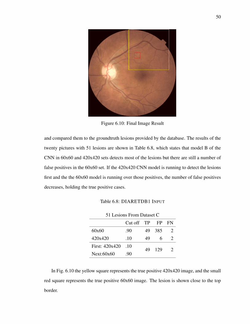
50
Figure 6.10: Final Image Result
and compared them to the groundtruth lesions provided by the database. The results of the
twenty pictures with 51 lesions are shown in Table 6.8, which states that model B of the
CNN in 60x60 and 420x420 sets detects most of the lesions but there are still a number of
false positives in the 60x60 set. If the 420x420 CNN model is running to detect the lesions
first and the the 60x60 model is running over those positives, the number of false positives
decreases, holding the true positive cases.
Table 6.8: DIARETDB1 INPUT
51 Lesions From Dataset C
Cut off TP FP FN
60x60 .90 49 385 2
420x420 .10 49 6 2
First: 420x420 .1049 129 2
Next:60x60 .90
In Fig. 6.10 the yellow square represents the true positive 420x420 image, and the small
red square represents the true positive 60x60 image. The lesion is shown close to the top
border.
51
CHAPTER 7
DISCUSSION
Qualitative improvement of the image not only facilitates the detection of the lesions
for annotations, but also decreases the number of epochs needed to reach a high accuracy
for training and validation sets. The benefits of shortening the training time are economic,
environmental, and human and can be reflected in the cost reduction. Because the color of
microaneurysms are located between 650-570 nm in the light spectrum and it is not possible
to find cyan colored microaneurysms, color reduction plays a significant role in medical
images where its variance is limited. As an illustration, the function in equation 5.3 was
successfully applied to enhance the lesions and provide contrast against their surroundings.
Quantitative gain either by augmentation or with new images makes the process more
accurate. Deep learning is very dependent of the size of the data. However, sometimes
the data-sets are limited, so augmentation was introduced to overcome this difficulty. Al-
though augmentation increased the accuracy of the study, adding new images had the same
effect, but with a lower number of images. Using Dataset C, we achieved a better accuracy
compared to Dataset B, but the increase in the accuracy was not as high as the one be-
tween Dataset A and B. This provides evidence that augmentation has a limit in improving
accuracy, but more studies are still needed.
The idea of having two different sized datasets (420x420 and 60x60) came from an old
medical tradition, which is explained as follows. Syphilis was a very dangerous disease in
the early 19th century, that later on had unpleasant complications. Epidemiologists came
up with the idea of a test (VDRL) that would detect all the cases of the disease. However,
52
it would produce a lot of false positives. The patient, whose VDRL test was positive, re-
quired a second test named (FTA-ABS), which had a specificity that was almost perfect,
but without a high sensitivity. Economic, logistic, and epidemiological reasons support
this approach. Although we used the same methodology, CNN, for both sets (60x60 and
420x420) they differ in the model and input size. As a result, these models could be con-
sidered different types of tests. The efforts in the study to increase the sensitivity in the
420x420 set by increasing the input size and implementing feedback were well paid off
by diminishing the false positives generated, when CNNs were applied to cropped images
with a size of 60x60 pixels as a unique test.
Most of the DR studies have been focused on classifying its stages, rather than iden-
tifying the specific lesion. R-CNN, Fast R-CNN,and Faster R-CNN have been used for
object localization with excellent results, but this still has not solved the problem for small
objects. Karphaty [47], introduced the idea of foveal stream for video classification by
cropping the image stream into its center. Grinsven’s work [20] developed a selective data
sampling for the detection of hemorrhages, where the lesions were placed in the center of
a cropped image of 41x41 pixels. Although the fovea in the retina has a more concentrated
area with photo-receptors, it is the attention that defines the discrimination of the objects.
In a similar way, we proposed that keeping the same resolution of the image, but cropping
the image to the object of interest would simulate the attention. Cropping the image with
the lesion in different positions of the image gives the input data a higher variance. We also
made sure to avoid that the CNN would learn the center position instead of the features of
the lesion itself.
In the 420x420 set, applying feedback to the CNN performed better than vanilla and
dropout increasing. Most of the chemical or physiological pathways have a feedback mech-
anism to regulate its response to a specific stimulus. Our approach tried to find the batch
with mild and normal classes that perform poorly after back-propagation to retrain them

53
again. One of the limitations of this approach was that we needed to know the values of the
loss function per batch during all of the training in order to calculate the function. However,
it is possible that a dynamic process can be created using a number of previous batches to
get the threshold and update it after a certain number of batches. Grinsven’s work [20]
proposed a feedback method that assigns a probability score to each pixel and is modified
when ”the probability scores differs the most from the initial reference level”,so the higher
the weight probability the higher the chance of it being selected. One drawback of this
methodology is that it is only applied to the negative sample.
Some observations that called the our group’s attention was that the CNN selected some
small artifacts as lesions. Also, the algorithms selected small groups of lesions, but when
a bigger number of lesions were grouped in such a way that they mimic hemorrhages,
they were not detected. Although we gained some progress in the detection and selection
of microaneurysms and our technique’s performance surpassed all of the methods in the
literature at this time, there are still a number of false positives.
54
CHAPTER 8
CONCLUSIONS
This study proposed a novel methodology for pre-processing images that would de-
crease the training time and improve the quality of the images for annotations. Normal-
ization is the first step in image pre-processing that generates an image with a mean value
closer to the mean value of all of the images, and with a standard deviation value bigger
than its original value. The second step adjusts the luminescence of the images, so that the
dark and white regions would be more visually appealing. The final step is color reduc-
tion,where the intensity of the pixels of the colors is moved within the spectrum between
the yellow and orange intensity. The new intensity of the pixels’ image is similar to either
the vessel color or to the background color.
Also, the study reaffirms that deep learning is data dependent and obtain new data is
as important as augmentation. Some datasets have a limited number of cases that need to
be trained by a Deep Learining algorithm. Augmentation is a methodology that overcomes
this limitation, and has been used successfully in several studies. The study showed that
augmentation has a limitation when improving accuracy and adding new cases to the data
set and performs better than using augmentation. Therefore, in future studies augmentation
should be used in a cautionary manner.
The study offered new feedback methodology for training that improves accuracy in
the 420x420 testing set. Finally, the study proposed a novel methodology by using a mul-
tiscale CNN model that increases the performance for identification and classification of
microanuerysms, which represent small sections of of the scene. Thus, this study combined

55
a CNN with a high sensitivity and a CNN with a high specificity to detect microaneurysms
with a few false positives. CNN trained with images that have a size of 60 × 60 pixels
to detect mycroaneurysms, artifacts, and hemorrhages. In addition, a CNN trained with
images that have a size of 60 × 60 pixels detected normal areas in our eyes, but they had
some features that triggered the CNN. On the other hand, a CNN trained with images hav-
ing a size of 420 × 420 pixels possessed a bigger area that makes it difficult to distinguish
small lesions from normal lesions. However, the study reached a sensitivity of 91% and
specificity of 93% for this CNN. This study used both CNNs sequentially to obtain our
more accurate results.
56
APPENDIX A
SOFTWARE IMPLEMENTATION
Image preprocessing helped to reduce the training time measured by the number of
epochs need to have the highest accuracy during training. Also, preprocessing helps the
author to make annotations in the images. The next section describes the manner our re-
search group implemented the algorithms explain in the methods chapter.
A.1 Preprocessing
For the study a well known, popular, good quality, and open source framework was
chosen,OpenCV. API’s framework provides several classes for loading, transform, conver-
sion, and drawing images, and we took advance of them. Also a simple GUI to display the
results of the operation and trackbars to make dynamic changes are available in this frame
work. Initially the image is loaded from a file; OpenCV provides MAT class to storage the
image as shown in the line 3.
1 string im= "image name";
2 Mat image;
3 image = imread(im);
After loading the image, conversion to float values is performed in the line 5. Then,
color space transformation from RGB to L∗, a∗, b∗ is showed in the line 6. The values
of the means and standard deviation of all pictures, and for each channel are assigned to
variables as depicted in the lines 7 to 12. In the lines 14 to 19 variables holding the mean
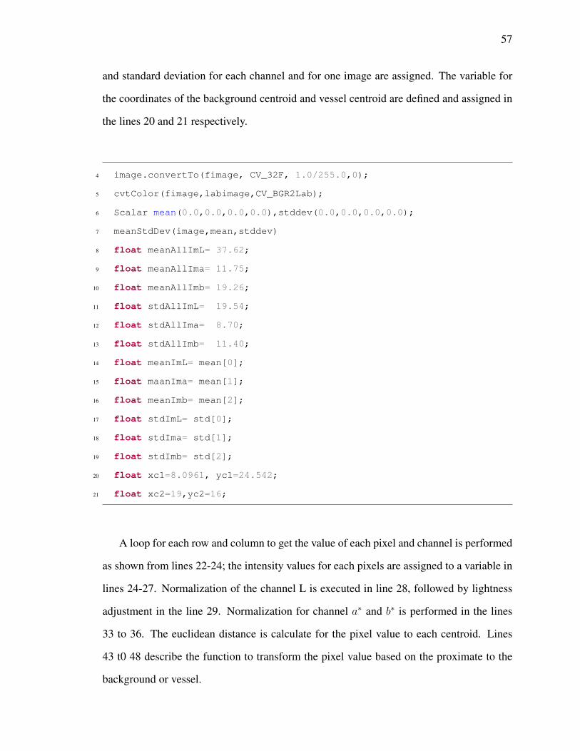
57
and standard deviation for each channel and for one image are assigned. The variable for
the coordinates of the background centroid and vessel centroid are defined and assigned in
the lines 20 and 21 respectively.
4 image.convertTo(fimage, CV_32F, 1.0/255.0,0);
5 cvtColor(fimage,labimage,CV_BGR2Lab);
6 Scalar mean(0.0,0.0,0.0,0.0),stddev(0.0,0.0,0.0,0.0);
7 meanStdDev(image,mean,stddev)
8 float meanAllImL= 37.62;
9 float meanAllIma= 11.75;
10 float meanAllImb= 19.26;
11 float stdAllImL= 19.54;
12 float stdAllIma= 8.70;
13 float stdAllImb= 11.40;
14 float meanImL= mean[0];
15 float maanIma= mean[1];
16 float meanImb= mean[2];
17 float stdImL= std[0];
18 float stdIma= std[1];
19 float stdImb= std[2];
20 float xc1=8.0961, yc1=24.542;
21 float xc2=19,yc2=16;
A loop for each row and column to get the value of each pixel and channel is performed
as shown from lines 22-24; the intensity values for each pixels are assigned to a variable in
lines 24-27. Normalization of the channel L is executed in line 28, followed by lightness
adjustment in the line 29. Normalization for channel a∗ and b∗ is performed in the lines
33 to 36. The euclidean distance is calculate for the pixel value to each centroid. Lines
43 t0 48 describe the function to transform the pixel value based on the proximate to the
background or vessel.

58
22 for (int i = 0; i < labimage.rows; i++){
23 float* data=labimage.ptr<float>(i);
24 for (int j = 0; j < labimage.cols ; j++){
25 float d0=(data[(3*j)+0]);
26 float d1=(data[(3*j)+1]);
27 float d2=(data[(3*j)+2]);
28 float tmpl = (((d0-m0)*((sumstddev[0]/s[0])*2))+m0)+(summean[0]-m0);
29 float tmp2 = (pow(tmpl,3) * 0.0000056656) -(pow(tmpl,2) *
30 0.0015297)+ (tmpl*0.7973646)+ 9.83683 ;
31 float tmpa = (((d1-m1)*(sumstddev[1]/s[1]))+m1)+ (summean[1]-m1);
32 float tmpb = (((d2-m2)*(sumstddev[2]/s[2]))+m2)+(summean[2]-m2);
33 float r1= pow((pow((tmpa-xc1),2)) + (pow((tmpb-yc1),2)),0.5);
34 float r2= pow((pow((tmpa-xc2),2)) + (pow((tmpb-yc2),2)),0.5);
35 float rel=pow((r1/r2),4);
36 data[(3*j)+0]=tmp2;
37 if (rel <= 1){
38 data[(3*j)+1]= ((tmpa-xc1)*rel)+xc1;
39 data[(3*j)+2]= ((tmpb-yc1)*rel)+yc1;
40 }else{
41 data[(3*j)+1]= ((tmpa-xc2)/rel)+xc2;
42 data[(3*j)+2]= ((tmpb-yc2)/rel)+yc2;
43 }
44 }
45 }
59
REFERENCES
[1] M. Yanoff and J. S. Duker, Ophthalmology. Edinburgh: Mosby, 2008.
[2] C. P. Wilkinson, F. L. I. Ferris, R. E. Klein, P. P. Lee, C. D. Agardh, M. Davis, D.Dills, A. Kampik, R. Pararajasegaram, and J. T. Verdaguer, “Proposed internationalclinical diabetic retinopathy and diabetic macular edema disease severity scales,”Ophthalmology, vol. 110, no. 9, pp. 1677–1682, 2003.
[3] Y. LeCun, O. Matan, B. Boser, J. S. Denker, D. Henderson, R. E. Howard, W. Hub-bard, L. D. Jackel, and H. S. Baird, “Handwritten zip code recognition with mul-tilayer networks,” in Proc. of the International Conference on Pattern Recognition,IAPR, Ed., invited paper, vol. II, Atlantic City: IEEE, 1990, pp. 35–40.
[4] A. Krizhevsky, I. Sutskever, and G. E. Hinton, “Imagenet classification with deepconvolutional neural networks,” in Advances in Neural Information Processing Sys-tems 25, F. Pereira, C. Burges, L. Bottou, and K. Weinberger, Eds., Curran Asso-ciates, Inc., 2012, pp. 1097–1105.
[5] K. Simonyan and A. Zisserman, “Very deep convolutional networks for large-scaleimage recognition,” CoRR, vol. abs/1409.1556, 2014.
[6] S. Zagoruyko and N. Komodakis, “Wide residual networks,” CoRR, 1999. arXiv:1605.07146 [cs.CV].
[7] C. Szegedy, W. Liu, Y. Jia, P. Sermanet, S. Reed, D. Anguelov, D. Erhan, V. Van-houcke, and A. Rabinovich, “Going deeper with convolutions,” CoRR, 1999. arXiv:1409.4842 [cs.CV].
[8] X. Glorot and Y. Bengio, “Understanding the difficulty of training deep feedforwardneural networks,” JMLR, 2010.
[9] S. Ioffe and C. Szegedy, “Batch normalization: Accelerating deep network trainingby reducing internal covariate shift,” CoRR, 1999. arXiv: 1502.03167 [cs.LG].
[10] I. J. Goodfellow, D. Warde-Farley, M. Mirza, A. C. Courville, and Y. Bengio, “Max-out networks,” CoRR, vol. abs/1302.4389, 2013.
[11] H. Su, F. Liu, Y. Xie, F. Xing, S. Meyyappan, and L. Yang, “Region segmentationin histopathological breast cancer images using deep convolutional neural network,”
60
in 2015 IEEE 12th International Symposium on Biomedical Imaging (ISBI), 2015,pp. 55–58.
[12] E. E. Nithila and S. Kumar, “Automatic detection of solitary pulmonary nodulesusing swarm intelligence optimized neural networks on {ct} images,” EngineeringScience and Technology, an International Journal, pp. –, 2016.
[13] V. Gulshan, L. Peng, M. Coram, M. C. Stumpe, D. Wu, A. Narayanaswamy, S. Venu-gopalan, K. Widner, T. Madams, J. Cuadros, R. Kim, R. Raman, P. C. Nelson, J. L.Mega, and D. R. Webster, “Development and validation of a deep learning algorithmfor detection of diabetic retinopathy in retinal fundus photographs,” JAMA, vol. 316,no. 22, p. 2402, 2016.
[14] M.Sankar, K.Batri, and R.Parvathi, Earliest diabetic retinopathy classification usingdeep convolution neural networks.pdf, 2016.
[15] H. Pratt, F. Coenen, D. M. Broadbent, S. P. Harding, and Y. Zheng, “Convolutionalneural networks for diabetic retinopathy,” Procedia Computer Science, vol. 90, no.nil, pp. 200–205, 2016.
[16] G. Lim, M. L. Lee, W. Hsu, and T. Y. Wong, Transformed representations for con-volutional neural networks in diabetic retinopathy screening, 2014.
[17] N. Petrick, H.-P. Chan, B. Sahiner, and D. Wei, “An adaptive density-weighted con-trast enhancement filter for mammographic breast mass detection,” IEEE Transac-tions on Medical Imaging, vol. 15, no. 1, pp. 59–67, 1996.
[18] F. C. Ghesu, B. Georgescu, Y. Zheng, J. Hornegger, and D. Comaniciu, “Marginalspace deep learning: Efficient architecture for detection in volumetric image data,”in Medical Image Computing and Computer-Assisted Intervention – MICCAI 2015:18th International Conference, Munich, Germany, October 5-9, 2015, Proceedings,Part I, N. Navab, J. Hornegger, W. M. Wells, and A. F. Frangi, Eds. Cham: SpringerInternational Publishing, 2015, pp. 710–718, ISBN: 978-3-319-24553-9.
[19] T. Brosch, Y. Yoo, L. Y. W. Tang, D. K. B. Li, A. Traboulsee, and R. Tam, “Deepconvolutional encoder networks for multiple sclerosis lesion segmentation,” in Med-ical Image Computing and Computer-Assisted Intervention – MICCAI 2015: 18thInternational Conference, Munich, Germany, October 5-9, 2015, Proceedings, PartIII, N. Navab, J. Hornegger, W. M. Wells, and A. F. Frangi, Eds. Cham: SpringerInternational Publishing, 2015, pp. 3–11, ISBN: 978-3-319-24574-4.
[20] M. J. J. P. van Grinsven, B. van Ginneken, C. B. Hoyng, T. Theelen, and C. I.Sanchez, “Fast convolutional neural network training using selective data sampling:Application to hemorrhage detection in color fundus images,” IEEE Transactions onMedical Imaging, vol. 35, no. 5, pp. 1273–1284, 2016.
61
[21] C. Bishop, Pattern recognition and machine learning. New York, NY: Springer,2006, ISBN: 978-0-387-31073-2.
[22] F. Rosenblatt, “The perceptron: A probabilistic model for information storage andorganization in the brain.,” Psychological Review, vol. 65, no. 6, pp. 386–408, 1958.
[23] P. J. Werbos, “Beyond regression: New tools for prediction and analysis in the be-havioral sciences,” PhD thesis, Harvard University, 1974.
[24] Definition of a neural network, http://uhaweb.hartford.edu/compsci/neural-networks-definition.html, Accessed:2017.
[25] D. E. Rumelhart, G. E. Hinton, and R. J. Williams, “Learning representations byback-propagating errors,” Nature, vol. 323, no. 6088, pp. 533–536, 1986.
[26] Artificial neural network, https://en.wikipedia.org/wiki/Artificial_neural_network, Accessed:2017, 2017.
[27] I. Goodfellow, Y. Bengio, and A. Courville, Deep Learning. MIT Press, 2016, http://www.deeplearningbook.org.
[28] K. Fukushima, “Neocognitron: A self-organizing neural network model for a mech-anism of pattern recognition unaffected by shift in position,” Biological Cybernetics,vol. 36, no. 4, pp. 193–202, 1980.
[29] Y. LeCun, B. Boser, J. S. Denker, D. Henderson, R. E. Howard, W. Hubbard, andL. D. Jackel, “Backpropagation applied to handwritten zip code recognition,” NeuralComputation, vol. 1, no. 4, pp. 541–551, 1989.
[30] Y. LeCun, Y. Bengio, and G. Hinton, “Deep learning,” Nature, vol. 521, no. 7553,pp. 436–444, 2015.
[31] A. Deshpande, A beginner’s guide to understanding convolutional neural networkspart 2, url=https://adeshpande3.github.io/adeshpande3.github.io/A-Beginner’s-Guide-To-Understanding-Convolutional-Neural-Networks-Part-2/, Accessed:2017.
[32] Y. LeCun, L. Bottou, Y. Bengio, and P. Haffner, “Gradient-based learning applied todocument recognition,” in Intelligent Signal Processing, IEEE Press, 2001, pp. 306–351.
[33] A. Krizhevsky, I. Sutskever, and G. E. Hinton, “Imagenet classification with deepconvolutional neural networks,” in Advances in Neural Information Processing Sys-tems, p. 2012.
62
[34] C. Szegedy, V. Vanhoucke, S. Ioffe, J. Shlens, and Z. Wojna, “Rethinking the incep-tion architecture for computer vision,” CoRR, 1999. arXiv: 1512.00567 [cs.CV].
[35] J. Jin, A. Dundar, and E. Culurciello, “Flattened convolutional neural networks forfeedforward acceleration,” CoRR, 1999. arXiv: 1412.5474 [cs.NE].
[36] K. He, X. Zhang, S. Ren, and J. Sun, “Deep residual learning for image recognition,”CoRR, 1999. arXiv: 1512.03385 [cs.CV].
[37] N. Srivastava, G. E. Hinton, A. Krizhevsky, I. Sutskever, and R. Salakhutdinov,“Dropout: A simple way to prevent neural networks from overfitting.,” Journal ofMachine Learning Research, vol. 15, no. 1, pp. 1929–1958, 2014.
[38] T. Fawcett, “An introduction to roc analysis,” Pattern Recognition Letters, vol. 27,no. 8, pp. 861–874, 2006.
[39] M. Mahy, L. Van Eycken, and A. Oosterlinck, “Evaluation of uniform color spacesdeveloped after the adoption of cielab and cieluv,” Color Research And Application,vol. 19, no. 2, 1994.
[40] Https://www.zeiss.com/spectroscopy/solutions-applications/color-measurement.html.Carl Zeiss Spectroscopy GmbH.
[41] R. L. Thorndike, “Who belongs in the family?” Psychometrika, vol. 18, no. 4, pp. 267–276, 1953.
[42] “Deep image: Scaling up image recognition,” CoRR, vol. abs/1501.02876, 2015,Withdrawn.
[43] B. Graham, “Fractional max-pooling,” CoRR, vol. abs/1412.6071, 2014.
[44] A. L. Maas, A. Y. Hannun, and A. Y. Ng, “Rectifier nonlinearities improve neu-ral network acoustic models,” in In ICML Workshop on Deep Learning for Audio,Speech and Language Processing, 2013.
[45] B. Xu, N. Wang, T. Chen, and M. Li, “Empirical evaluation of rectified activationsin convolutional network,” CoRR, vol. abs/1505.00853, 2015.
[46] K. He, X. Zhang, S. Ren, and J. Sun, “Delving deep into rectifiers: Surpassinghuman-level performance on imagenet classification,” CoRR, 1999. arXiv: 1502.01852 [cs.CV].
[47] A. Karpathy, G. Toderici, S. Shetty, T. Leung, R. Sukthankar, and L. Fei-Fei, “Large-scale video classification with convolutional neural networks,” in Proceedings of the2014 IEEE Conference on Computer Vision and Pattern Recognition, ser. CVPR

63
’14, Washington, DC, USA: IEEE Computer Society, 2014, pp. 1725–1732, ISBN:978-1-4799-5118-5.