Abstract—We proposed a technique to identify road traffic

congestion levels from velocity of mobile sensors with high accuracy and consistent with motorists’ judgments. The data collection utilized a GPS device, a webcam, and an opinion survey. Human perceptions were used to rate the traffic congestion levels into three levels: light, heavy, and jam. Then the ratings and velocity were fed into a decision tree learning model (J48). We successfully extracted vehicle movement patterns to feed into the learning model using a sliding windows technique. The model achieved accuracy as high as 91.29%. By implementing the model on the existing traffic report systems, the reports will cover on comprehensive areas. The proposed method can be applied to any parts of the world.

Index Terms—intelligent transportation system (ITS), traffic congestion level, human judgment, decision tree (J48), geographic positioning system (GPS).

I. INTRODUCTION Traffic reports in real-time are essential for congested and overcrowded cities such as Bangkok or even in sparse and remote areas during a long holiday period. Without these, commuters might not choose the proper routes and could get stuck in traffic for hours. Intelligent Transportation System (ITS) with automated congestion estimation algorithms can help produce such reports. Several initiatives from both private and government entities have been proposed and implemented to gather traffic data to feed the ITS. According to our survey, most efforts focus on limited installation of fixed sensors such as loop-coils and intelligent video cameras with image processing capability. However, the costs of such implementations are very high due to the high cost of the devices, installation, and maintenance. Moreover, these fixed sensors are vulnerable to extreme weather typical in certain areas. Additionally, the installation of fixed sensors to cover all roads in major cities is neither practical nor economically feasible. An alternative way to collect traffic data at a lower cost with wider coverage is therefore needed.

This work was supported by the National Electronics and Computer Technology Center (NECTEC), Thailand.

W. Pattara-Atikom is with the National Electronics and Computer Technology Center (NECTEC), under the National Science and Technology Development Agency (NSTDA), Ministry of Science and Technology, 112 Thailand Science Park, Phahon Yothin Rd., Klong 1, Klong Luang, Pathumthani 12120, Thailand (phone: +662-564-6900 ext. 2528, e-mail: wasan@nectec.or.th).

T. Thianniwet and S. Phosaard are with the School of Information Technology, Institute of Social Technology, Suranaree University of Technology, 111 University Ave., Muang Nakhon Ratchasima, Nakhon Ratchasima 30000, Thailand. (e-mail: thammasak@sut.ac.th and s@sut.ac.th).

Recently, mobile sensors or probe vehicles appeared as a

complementary solution to fixed sensors for increasing coverage areas and accuracy without requiring expensive infrastructure investment. Two popular types of mobile sensors are GPS-based and cellular-based. GPS-based sensors are sensors with GPS capability and cellular-based sensors are sensors that use information from cellular networks as traffic sensors.

Cellular-based sensors are low in cost due to the large number of mobile phones and their associated infrastructures already in service. According to recent statistics, the mobile phone penetration rate in Thailand is expected to grow to 90% in 2009 [1]. However, GPS-based sensors are far more efficient to pinpoint vehicle locations, thus they can provide highly accurate vehicle movement information. Moreover, recent mobile phones have integrated GPS capability, such as Apple iPhone and several other smart phones.

In this paper, we explored a model that can automatically classified traffic congestion levels for traffic reports. The model can be further implemented in the system that combines advantages of GPS-based sensors, in that they are highly accurate, and of cellular-based sensors, in that they are highly available. This model, combine with mobile sensors, can generate traffic reports that virtually cover all of the areas that vehicles and mobile networks can reach.

This paper is organized as follows: In Section II, we describe related works concerning traffic congestion reports. The methodology of the research is presented in Section III. Section IV provides results and evaluations, and Section V offers a conclusion and the possibilities of future work.

II. RELATED WORKS Congestion level estimation techniques for various types

of the collected data are our most related field. Traffic data could be gathered automatically from two major types of sensors: fixed sensor and mobile sensor. The study in [2] applied the neural network technique to the collected data using mobile phones. It used Cell Dwell Time/CDT, the time that a mobile phone attaches to a mobile phone service antenna, which provides rough journey speed. Our work employed another machine learning technique that was better suit with the characteristics of the data. The GPS data would provide more precise traffic information than that roughly provided by the CDT. The studies in [3] and [4] estimated the congestion level using data from traffic camera by applying fuzzy logic and hidden Markov model, respectively. Our work applied decision tree (J48) technique

Classification of Road Traffic Congestion Levels from GPS Data using a Decision Tree

Algorithm and Sliding Windows Thammasak Thianniwet, Satidchoke Phosaard, member, IAENG, and Wasan Pattara-Atikom

Proceedings of the World Congress on Engineering 2009 Vol IWCE 2009, July 1 - 3, 2009, London, U.K.

ISBN: 978-988-17012-5-1 WCE 2009

on mobile sensors. Using data collected from mobile sensors would cover far greater traffic ranges. The algorithm would learn over movement patterns of a vehicle. Sliding window technique with fixed window size was also used. The works of [5], [6] and [7] also investigated various alternative techniques related to our work.

In some countries, for example, as in the study of [8] and [9] found out that the main parameters used to define the traffic congestion levels are time, speed, volume, service level, and the cycles of traffic signal that the motorists have to wait. Our work would focus only on interpretation of vehicle velocity since our work needs to determine the congestion levels with minimal parameters. Vehicle velocity could be collected by almost all types of sensors. This made it easier, broader and more versatile for the model to be used. The congestion levels that we studied were limited to three levels: free-flow, heavy and jam, which was enough and appropriate according to the study of [10]. After we successfully derived the congestion classification model, the GPS data were planned to be collected through mobile phones attached by GPS device. The data would be sent through the data network, such as GPRS, EDGE, and so on. The next section described the methodology of the research.

III. METHODOLOGY

A. Collection of Empirical Data The traffic data were collected from several highly

congested roads in Bangkok, e.g., Sukhumvit, Silom, and Sathorn. A notebook attached with a USB GPS device is used to collected date, time, latitude, longitude, and vehicle velocity from GPS’s GPRMC sentences. We captured images of road traffic condition by a video camera mounted on a test vehicle’s dash board. Our vehicle passed through overcrowded urban areas approximately 30 kilometers within 3 hours.

In our experiment, we gathered the congestion levels from 11 subjects with driving experience up to 10 years. They watched a 3-hour video clip of road survey and rated the congestion levels into three levels, light, heavy, and jam. Then, the concluded congestion levels from 11 subjects were calculated using majority vote. The judged congestion levels were then synchronized with velocity collected by the GPS device. We observed that the data were wildly fluctuated and also non-uniform, as shown in Fig. 1. To alleviate this oscillation, the traffic data was treated before feeding into a learning algorithm, i.e., decision tree model, which will be explained in detail in the next section.

B. Data Preparation We minimized a set of attributes by concentrating only on

the vehicle velocity and the moving pattern of a vehicle, which can infer different levels of congestion. Then, we applied three steps to prepare the data: 1) smoothening out instantaneous velocity, 2) extracting moving pattern of a vehicle using sliding windows technique, and 3) balancing the distribution of sampling data on each congestion level. Next, we will explain each procedure in details.

1) Smoothening Out Instantaneous Velocity Instantaneous vehicle velocity from the GPS data usually

fluctuated widely, as shown in Fig. 1 as the dotted line. This fluctuation made the learning algorithm difficult to determine the pattern and classify the congestion level, as in [11]. Therefore, we needed to smoothen out the fluctuation of instantaneous velocity. We applied moving average algorithm by averaging the previous ξ samples as shown in Eq. 1. MVt represents the moving average velocity at time t. In our experiment, ξ was set to 3. The results of the average velocity are shown as the thick line in Fig. 1.

ξ

ξiVt

titMV

−=∑

= (1)

Fig. 1. Instantaneous velocity vs. moving average velocity

(ξ = 3)

2) Extracting Vehicle’s Moving Patterns When the instantaneous velocity was less fluctuated by

the smoothening algorithm, it was easier to investigate vehicle’s moving patterns. We successfully extracted moving patterns that were practical to be efficiently learned by the learning algorithm, which can be explained as follows. Our previous work suggested we can use velocity to estimate congestion levels. For example, Fig. 2 illustrates the vehicle moving patterns corresponding to the congestion levels. To make the graph readable, we scale the congestion scores (1, 2 and 3) by 10, i.e., 10 = jam, 20 = heavy and 30 = light.

Proceedings of the World Congress on Engineering 2009 Vol IWCE 2009, July 1 - 3, 2009, London, U.K.

ISBN: 978-988-17012-5-1 WCE 2009

Fig. 2. Vehicle moving pattern and deduced congestion level

From Fig 2, when a vehicle is moving with high velocity for a while, it means that the road traffic is light, e.g., the velocity between the time of 10 and 14. If the velocity decreases to a moderate range, it means that the road traffic is heavy, e.g., the velocity at the time of 15. And if the velocity decreases to low velocity, it means that the road traffic is jam.

Although, the value of vehicle velocity can be used to determine the congestion level, we cannot say that only a value of the vehicle velocity at a moment can be used to accurately determine the congestion level. In a real driving situation, an instantaneous velocity can be reporated at any congestion levels. For example, a vehicle needs to slow down for turning or stopping for a traffic light. In this condition, the traffic might be light but the velocity is relatively low. Fig. 3 visualizes the data space between congestion levels and instantaneous velocity. For example, the reported congestion levles of the velocity near 0 km/h, they were mutally reported as either light, heavy or jam.

  x = 1 (jam)        x = 2 (heavy)        x = 3 (light)

Inst

ance

s Con

gest

ion

Lev

el

Instantaneous Velocity (km/h)

Fig. 3. Congestion levels vs. instantaneous velocity

After carefully investigating the data, we succesfully mimicked humans’ judements on congestion levels based on moving patterns of a vehicle which was derived from the historical data. Sliding windows, a technique that could satisfy such moving pattern extraction, was employed. We applied fixed sliding windows of size δ to capture moving patterns of a vehicle from the vehicle velocity. In our experiment, δ was set to 3, which means we captured the moving patterns by a set of three consecutive moving average velocities. The moving pattern at time t with δ equals to 3 includes three consecutive samples of moving average velocity at time t (MVt), and two priori moving average velocities at time t-1 (MVt-1), and t-2 (MVt-2). We also introduced a new attribute to represent the average velocity of each sliding window (each moving pattern), called AMVt. For the moving pattern at time t with δ and ξ set to 3, the value of AMVt can be computed by the value of MVt (ξ = 5). Table I demonstrates how to calculate the moving average at time t from instantaneous velocity (INSt), and how to extract moving patterns.

The steps of how to calculate the values in Table I can be explained as follows. The moving average velocity by the

time of 13:12 can be calculated by averaging the current instantaneous velocity, 42.06, with two priori velocity, 27.79 and 44.66. AMVt is the average velocity which covers the moving pattern at time t. The value of AMVt at 13:14 can be calculated by averaging instantaneous velocity beginning from 13:10, also a starting point of MVt-2, to 13:14, also the end point of MVt. Thus, the calculation of an AMVt with δ and ξ set to 3 equals to the calculation of an MVt with ξ set to 5. The last column, Level, indicates congestion levels rated by human. The values of 1, 2, and 3 represent jam, heavy, and light traffic respectively.

TABLE I

AN EXAMPLE OF INSTANTANEOUS VELOCITY AND DERIVED ATTRIBUTES Time INSt MVt-2 MVt-1 MVt AMVt Level 13:10 44.66 - - - - 3 13:11 27.79 - - - - 3 13:12 42.06 - - 38.17 - 3 13:13 55.09 - 38.17 41.65 - 3 13:14 29.83 38.17 41.65 42.33 39.89 3 13:15 2.04 41.65 42.33 28.99 31.36 2 13:16 1.11 42.33 28.99 10.99 26.03 1 13:17 14.45 28.99 10.99 5.87 20.50 1

3) Balancing Class Distributions In our experiment, we captured vehicle’s moving patterns

every minute from 13:00 to 15:45. Since the calculations of MVt and AMVt depend on previous cascading calculations, the first four instances were omitted. Therefore, there were 162 instances: 52 instances were in the class of jam traffic, 74 instances were in the class of heavy traffic, and there were only 36 instances were in the class of light traffic. Class imbalance may cause inferior accuracy in data mining learners, as [12]. Generally, classification models tend to predict the majority class if class imbalance exists. In this case, the class of heavy traffic was the majority class while the minority classes, the classes of light and jam traffic, were also highly important. Therefore, we needed to balance the class distributions to avoid the problem.

By this step, we applied a simple technique to alleviate the problem of class imbalance by applying a technique that was similar to the technique of finding a least common multiple number. The result of class balancing yielded 448 instances with 156 instances on class jam, 148 instances on class heavy, and 144 instances on class light. Then, this data set was used to train the classification model, for which we explain the details in the next section.

C. Data Classifications The preprocessed data set was used to train and evaluate

the classification model. Our data set consisted of five attributes. The first three attributes were MV3t-2, MV3t-1, and MV3t, which were three consecutive moving average velocities that represented the moving pattern. The fourth attribute was AMV3t, which was the average velocity of the corresponding moving pattern. The last attribute was Level, which was the congestion level judged by human ratings. We chose the J48 algorithm, a well-known decision tree algorithm in the WEKA system, to generate a decision tree model to classify the Level. WEKA is a machine learning software developed by the University of Waikato. It is a collection of machine learning algorithms for data mining tasks. The goal attribute of the model was set to Level. The test option was set to 10-fold cross-validation.

Proceedings of the World Congress on Engineering 2009 Vol IWCE 2009, July 1 - 3, 2009, London, U.K.

ISBN: 978-988-17012-5-1 WCE 2009

Fig. 4 shows the knowledge flow, steps of generation and evaluation of the classification model, of our experiment.

ArffLoader

ClassAssigner CrossValidationFoldMaker

J48

TextViewer

GraphViewer

dataSet

trainingSettestSet

text

graphdataSet

batchClassifier

ClassifierPerformanceEvaluator

ModelPerformanceChart

visualizableError

Fig. 4. Knowledge flow of our experiment

IV. RESULTS AND EVALUATIONS

A. Classification Model After successfully training the classification model, the

derived decision tree is show in Fig 5. The size of our decision tree is 125 nodes, 63 of which are leave nodes. The time taken to build the model is about 0.08 seconds. The root node is AMV3t attribute. This means that the average of the moving average velocity is the most important factor to determine the level of road traffic congestion.

B. Performance Evaluations The result shows a promising technique of determining

congestion with an overall accuracy of 91.29%, a root mean square error of 0.2171, and a precision ranging from 0.882 to 0.966. The result shows a true positive rate (TP Rate or sensitivity) ranging from 0.777 to 1.000, which is very high, and a false positive rate (FP Rate) ranging from 0.013 to 0.068, which is very low. Table II shows the classifier’s

performance for each class in details. Table III shows the result of the model evaluation by a confusion matrix.

TABLE II

THE CLASSIFIER’S PERFORMANCE Class TP Rate FP Rate Precision

Jam (1) 0.962 0.068 0.882 Heavy (2) 0.777 0.013 0.966 Light (3) 1.000 0.049 0.906 Average 0.913 0.044 0.918

TABLE III

THE CONFUSION MATRIX

Predicted Congestion Level

Jam Heavy Light Jam 150 4 2

Heavy 20 115 13 Instances

Light 0 0 144

From Table II, the highest TP Rate is 1.000 on the Light

class. This means that when the road traffic congestion level is light, our classifier will 100% correctly classify the traffic. The lowest TP Rate is 0.777 on the Heavy class. It can be interpreted that when the road traffic congestion level is heavy, our classifier will 77.7% correctly classify the traffic. In general outlier human perceptions could occur. Because the heavily congested level is at the middle between the light and jam level, some people may judge the traffic in the light class or in the jam class as being in the heavy class. When these judgments were fed into the classification algorithm, they were treated as noise and would be ignored. The number 20 and 13 in the confusion matrix, as per Table III, is the result of misclassification on the heavy traffic class. The number 20 represents the instances of heavy class which the model misclassified as jam traffic, and the number 13 represents the instances in heavy class which the model misclassified as light traffic.

Fig. 5. The derived J48 decision tree

Proceedings of the World Congress on Engineering 2009 Vol IWCE 2009, July 1 - 3, 2009, London, U.K.

ISBN: 978-988-17012-5-1 WCE 2009

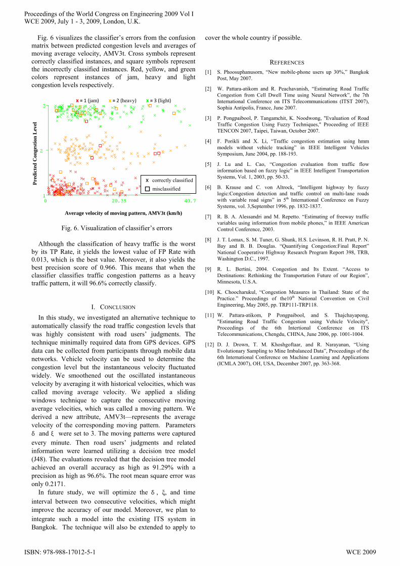
Fig. 6 visualizes the classifier’s errors from the confusion matrix between predicted congestion levels and averages of moving average velocity, AMV3t. Cross symbols represent correctly classified instances, and square symbols represent the incorrectly classified instances. Red, yellow, and green colors represent instances of jam, heavy and light congestion levels respectively.

  x = 1 (jam)        x = 2 (heavy)        x = 3 (light) 

Pred

icte

d C

onge

stio

n L

evel

Average velocity of moving pattern, AMV3t (km/h)

Fig. 6. Visualization of classifier’s errors

Although the classification of heavy traffic is the worst by its TP Rate, it yields the lowest value of FP Rate with 0.013, which is the best value. Moreover, it also yields the best precision score of 0.966. This means that when the classifier classifies traffic congestion patterns as a heavy traffic pattern, it will 96.6% correctly classify.

I. CONCLUSION In this study, we investigated an alternative technique to

automatically classify the road traffic congestion levels that was highly consistent with road users’ judgments. The technique minimally required data from GPS devices. GPS data can be collected from participants through mobile data networks. Vehicle velocity can be used to determine the congestion level but the instantaneous velocity fluctuated widely. We smoothened out the oscillated instantaneous velocity by averaging it with historical velocities, which was called moving average velocity. We applied a sliding windows technique to capture the consecutive moving average velocities, which was called a moving pattern. We derived a new attribute, AMV3t—represents the average velocity of the corresponding moving pattern. Parameters δ and ξ were set to 3. The moving patterns were captured every minute. Then road users’ judgments and related information were learned utilizing a decision tree model (J48). The evaluations revealed that the decision tree model achieved an overall accuracy as high as 91.29% with a precision as high as 96.6%. The root mean square error was only 0.2171.

In future study, we will optimize the δ , ξ, and time interval between two consecutive velocities, which might improve the accuracy of our model. Moreover, we plan to integrate such a model into the existing ITS system in Bangkok. The technique will also be extended to apply to

cover the whole country if possible.

REFERENCES [1] S. Phoosuphanusorn, “New mobile-phone users up 30%,” Bangkok

Post, May 2007.

[2] W. Pattara-atikom and R. Peachavanish, “Estimating Road Traffic Congestion from Cell Dwell Time using Neural Network”, the 7th International Conference on ITS Telecommunications (ITST 2007), Sophia Antipolis, France, June 2007.

[3] P. Pongpaibool, P. Tangamchit, K. Noodwong, "Evaluation of Road Traffic Congestion Using Fuzzy Techniques," Proceeding of IEEE TENCON 2007, Taipei, Taiwan, October 2007.

[4] F. Porikli and X. Li, “Traffic congestion estimation using hmm models without vehicle tracking” in IEEE Intelligent Vehicles Symposium, June 2004, pp. 188-193.

[5] J. Lu and L. Cao, “Congestion evaluation from traffic flow information based on fuzzy logic” in IEEE Intelligent Transportation Systems, Vol. 1, 2003, pp. 50-33.

[6] B. Krause and C. von Altrock, “Intelligent highway by fuzzy logic:Congestion detection and traffic control on multi-lane roads with variable road signs” in 5th International Conference on Fuzzy Systems, vol. 3,September 1996, pp. 1832-1837.

[7] R. B. A. Alessandri and M. Repetto. “Estimating of freeway traffic variables using information from mobile phones,” in IEEE American Control Conference, 2003.

[8] J. T. Lomax, S. M. Tuner, G. Shunk, H.S. Levinson, R. H. Pratt, P. N. Bay and B. B. Douglas. “Quantifying Congestion:Final Report” National Cooperative Highway Research Program Report 398, TRB, Washington D.C., 1997.

[9] R. L. Bertini, 2004. Congestion and Its Extent. “Access to Destinations: Rethinking the Transportation Future of our Region”, Minnesota, U.S.A.

[10] K. Choocharukul, “Congestion Measures in Thailand: State of the Practice.” Proceedings of the10th National Convention on Civil Engineering, May 2005, pp. TRP111-TRP118.

[11] W. Pattara-atikom, P Pongpaibool, and S. Thajchayapong, "Estimating Road Traffic Congestion using Vehicle Velocity", Proceedings of the 6th Intertional Conference on ITS Telecommunications, Chengdu, CHINA, June 2006, pp. 1001-1004.

[12] D. J. Drown, T. M. Khoshgoftaar, and R. Narayanan, “Using Evolutionary Sampling to Mine Imbalanced Data”, Proceedings of the 6th International Conference on Machine Learning and Applications (ICMLA 2007), OH, USA, December 2007, pp. 363-368.

   misclassifiedx   correctly classified

Proceedings of the World Congress on Engineering 2009 Vol IWCE 2009, July 1 - 3, 2009, London, U.K.

ISBN: 978-988-17012-5-1 WCE 2009