classifying polynomials of linear codes - mathematisch instituut
TRANSCRIPT
R.P.M.J. Jurrius
Classifying polynomialsof linear codes
Master thesis, defended on June 27, 2008
Thesis advisors: G.R. Pellikaan (TU/e)R. de Jong (UL)
Mathematisch Instituut, Universiteit Leiden

Contents
1 Introduction and definitions 5
1.1 Introduction . . . . . . . . . . . . . . . . . . . . . . . . . . . . 5
1.2 Definitions . . . . . . . . . . . . . . . . . . . . . . . . . . . . . 5
1.2.1 Linear codes . . . . . . . . . . . . . . . . . . . . . . . . 5
1.2.2 Weight distributions . . . . . . . . . . . . . . . . . . . 6
1.2.3 More about codes . . . . . . . . . . . . . . . . . . . . . 8
1.2.4 Matroids . . . . . . . . . . . . . . . . . . . . . . . . . . 9
1.2.5 Gaussian binomials and other products . . . . . . . . . 10
1.3 Notes . . . . . . . . . . . . . . . . . . . . . . . . . . . . . . . . 10
2 Weight enumerator 11
2.1 Generalized weight enumerator . . . . . . . . . . . . . . . . . 11
2.2 Extended weight enumerator . . . . . . . . . . . . . . . . . . . 15
2.3 Another algorithm . . . . . . . . . . . . . . . . . . . . . . . . 18
2.4 Generalized extended weight enumerator . . . . . . . . . . . . 21
2.5 Notes . . . . . . . . . . . . . . . . . . . . . . . . . . . . . . . . 23
3 Connections 25
3.1 Extended in terms of generalized . . . . . . . . . . . . . . . . 25
3.2 Generalized in terms of extended . . . . . . . . . . . . . . . . 27
3.3 Weight enumerator and Tutte polynomial . . . . . . . . . . . . 28
3.4 Overview . . . . . . . . . . . . . . . . . . . . . . . . . . . . . . 30
3.5 Notes . . . . . . . . . . . . . . . . . . . . . . . . . . . . . . . . 31
4 MacWilliams identities 33
4.1 Using the Tutte polynomial . . . . . . . . . . . . . . . . . . . 33
4.2 Generalized MacWilliams identities . . . . . . . . . . . . . . . 34
4.3 An alternative approach . . . . . . . . . . . . . . . . . . . . . 35
4.4 Notes . . . . . . . . . . . . . . . . . . . . . . . . . . . . . . . . 38
3
4 CONTENTS
5 Examples 395.1 MDS codes . . . . . . . . . . . . . . . . . . . . . . . . . . . . 395.2 Two [6, 3] codes . . . . . . . . . . . . . . . . . . . . . . . . . . 415.3 Notes . . . . . . . . . . . . . . . . . . . . . . . . . . . . . . . . 45
6 Implementation and complexity 476.1 About the computer implementation . . . . . . . . . . . . . . 476.2 The implementation . . . . . . . . . . . . . . . . . . . . . . . 486.3 Example: the ternary Golay code . . . . . . . . . . . . . . . . 516.4 Complexity calculations . . . . . . . . . . . . . . . . . . . . . 536.5 Notes . . . . . . . . . . . . . . . . . . . . . . . . . . . . . . . . 54
7 Conclusions 55
Chapter 1
Introduction and definitions
1.1 Introduction
The weight enumerator of a linear code is a classifying polynomial associatedwith the code. Besides its intrinsic importance as a mathematical object, it isused in the probability theory around codes. For example, the weight enumer-ator of a binary code is very useful if we want to study the probability that areceived message is closer to a different codeword than to the codeword sent.(Or, rephrased: the probability that a maximum likelihood decoder makes adecoding error.)We will generalize the weight enumerator in two ways, which lead to polyno-mials which are better invariants for a code. A procedure for the determina-tion of these polynomials is given. We will show that the two generalisationsdetermine each other, and that they connect to the Tutte polynomial of amatroid, thus linking coding theory and matroid theory. Most of the general-isations and connections have been studied before, but mostly only one-way,and a complete overview was never given.We will use the established connections to derive MacWilliams relations forour generalisations. Also other examples of the developed machinery will begiven, as well as a computer implementation.
1.2 Definitions
1.2.1 Linear codes
Definition 1.2.1 Let q be a prime power, and let Fq be the finite field with qelements. A linear subspace of Fn
q of dimension k is called a linear [n, k] codeand is usually denoted by C. The elements of the code are called (code)words.
5
6 CHAPTER 1. INTRODUCTION AND DEFINITIONS
A code can be given by writing down all elements, but because the code is alinear subspace, it has a basis.
Definition 1.2.2 The generator matrix of a linear [n, k] code C is a k × nmatrix of full rank over Fq whose rows form a basis of C.
Note that this matrix is not unique. We can rewrite the definition of a codein terms of the generator matrix:
C = {xG : x ∈ Fkq}.
A measurement for how much information is added by using a code, is theinformation rate:
Definition 1.2.3 The information rate of a linear [n, k] code is defined byR = k
n.
We will assume all our codes to be non-degenerate: there are no coordinateswhich are zero for al codewords, i.e. the generator matrix does not containany zero columns.
1.2.2 Weight distributions
For a word of a linear [n, k] code C, the (Hamming) weight is the numberof non-zero coordinates of the word. So the zero word has weight 0, andthe maximum possible weight is n, the length of the code. The (Hamming)distance between two codewords of C is the number of coordinates wherethe words differ. The minimum of all non-zero distances between codewordsis called the minimum distance. Because C is assumed to be linear, this isequal to the minimum non-zero weight of the code.We summarize all this in the following definition:
Definition 1.2.4 Let C be a linear [n, k] code and x,y ∈ Fnq . Then we define
wt(x) = |{i : xi 6= 0}|,
d(x,y) = |{i : xi 6= yi}|,
d = min{d(x,y) : x,y ∈ C,x 6= y} = min{wt(x) : x ∈ C,x 6= 0}.
The number of codewords c ∈ C with wt(c) = w is denoted by Aw. Notethat A0 = 1 and that d is the smallest w > 0 for which Aw > 0. The numbersAw for all 0 ≤ w ≤ n form the weight distribution of the code. They alsoform the coefficients of the weight enumerator :
1.2. DEFINITIONS 7
Definition 1.2.5 The weight enumerator of a linear [n, k] code C is thepolynomial
WC(X, Y ) =n∑
w=0
AwXn−wY w,
where Aw = |{c ∈ C : wt(c) = w}|.
Another way to define the weight enumerator is
WC(X, Y ) =∑c∈C
Xn−wt(c)Y wt(c).
We will always use this homogeneous form of the weight enumerator. Thereis also the one-variable form, WC(Z), which is connected to the homogeneousform via WC(X, Y ) = XnWC(Y X−1) and WC(Z) = WC(1, Z).
We can generalize the weight distribution in the following way. Instead oflooking at words of C, we consider all the subcodes of C of a certain dimensionr. We say that the weight of a subcode is equal to n minus the numberof coordinates which are zero for every word in the subcode. The smallestweight for which a subcode of dimension r exists, is called the r-th generalizedHamming weight of C. To summarize:
Definition 1.2.6 Let D be an r-dimensional subcode of the [n, k] code C.Then we define
wt(D) = |{i ∈ [n] : ∃x ∈ D : xi 6= 0}|,
dr = min{wt(D) : D ⊆ C subcode, dimD = r}.
Note that d0 = 0 and d1 = d, the minimum distance of the code. Thenumber of subcodes with a given weight w and dimension r is denoted byAr
w. Together they form the r-th generalized weight distribution of the code.Just as with the ordinary weight distribution, we can make a polynomialwith the distribution as coefficients: the generalized weight enumerator.
Definition 1.2.7 The generalized weight enumerator is given by
W rC(X, Y ) =
n∑w=0
ArwX
n−wY w,
where Arw = |{D ⊆ C : dimD = r,wt(D) = w}|.
8 CHAPTER 1. INTRODUCTION AND DEFINITIONS
We can see from this definition that A00 = 1 and Ar
0 = 0 for all 0 < r ≤ k.Furthermore, every 1-dimensional subspace of C contains q−1 non-zero code-words, so (q − 1)A1
w = Aw for 0 < w ≤ n.
If confusion about the underlying code is possible, we denote the code be-tween brackets behind the invariant: for example dr(C) or Aw(C⊥).
1.2.3 More about codes
Let < , > be the inner product on Fnq given by the symmetric linear form
< x,y >=∑n
i=1 xiyi. Then the dual code of a linear [n, k] code C over Fq isthe subspace of Fn
q orthogonal to C with respect to < , >.
Definition 1.2.8 Let C be a linear [n, k] code over Fq. Then the dual codeis
C⊥ = {x ∈ Fnq : < x, c >= 0 for all c ∈ C}.
It is clear that the dual code is again a linear code of length n over Fq andhas dimension n− k. Furthermore, (C⊥)⊥ = C.
There are two important bounds on the parameters of a code which we aregoing to use. For the proofs we refer to [8], [10] or any other course in basiccoding theory.
Theorem 1.2.9 (Singleton bound) Let C be a linear [n, k] code over Fq.Then d ≤ n− k + 1. �
Definition 1.2.10 (MDS code) A linear [n, k] code C is called maximumdistance separable if it achieves the Singleton bound, so if d = n− k + 1.
Theorem 1.2.11 (Gilbert–Varshamov bound) Fix integers q, n, d. Letk be the smallest integer satisfying
qk ≥ qn∑d−1i=0
(ni
)(q − 1)i
.
Then there exists a linear [n, k] code over Fq with minimum distance d. �
We will now define what it means for two codes to be equivalent. There areseveral ways to do this. The most easy one is to call two linear [n, k] codesover Fq equivalent if they are equal, i.e. if their row-space in Fn
q is the same.We are giving a more general definition, in order to let equivalent codescoincide with equivalent matroids and geometries.

1.2. DEFINITIONS 9
Definition 1.2.12 Two linear [n, k] codes over Fq are called equivalent iftheir generator matrices are the same up to
• left multiplication with an invertible k × k matrix over Fq;
• permutation of the columns;
• multiplication of columns with an element of F∗q.
Note that two equivalent codes have the same (generalized) weight distribu-tion.
1.2.4 Matroids
Matroid theory generalizes the notion of ‘independence’. We will use it formatrices over finite fields, but it also has important applications in otherbranches of combinatorics such as graph theory. There are many ways todefine a matroid: we will use a definition that makes it easy to see that thegenerator matrix of a linear code gives rise to a matroid.
Definition 1.2.13 A matroid G is a pair (S, I) where S is a finite set andI is a collection of subsets of S called the independent sets, satisfying thefollowing properties:
(i) The empty set is independent.
(ii) Every subset of an independent set is independent.
(iii) Let A and B be two independent sets with |A| > |B|, then there existsan a ∈ A with a /∈ B and B ∪ {a} an independent set.
A subset of S which is not independent, is called dependent. An independentsubset of S for which adding an extra element of S always gives a dependentsubset, is a maximal independent set or a basis. Just as in linear algebra,it can be showed that every basis has the same number of elements. This iscalled the rank of the matroid. We define the rank of a subset of S to be thesize of the largest independent set contained in it. For notation:
Definition 1.2.14 The rank r(A) of a matroid (S, I) and its set B of basesare defined by
r(A) = max{|A′| : A′ ⊆ A,A′ ∈ I}
B = {B ⊆ S : r(B) = |B| = r(S)}
10 CHAPTER 1. INTRODUCTION AND DEFINITIONS
The rank function and the set of bases can each be used to determine amatroid completely. Therefore we can define the dual of a matroid in thefollowing way:
Definition 1.2.15 Let G = (S,B) be a matroid defined by its set of bases.Then its dual is the matroid G∗ = (S,B∗) with the same underlying set andset of bases
B∗ = {S −B : B ∈ B}.
Note the similarity with the definition of a dual code. For a matroid we alsohave (G∗)∗ = G.
1.2.5 Gaussian binomials and other products
Definition 1.2.16 We introduce the following notations:
[m, r]q =r−1∏i=0
(qm − qi)
〈r〉q = [r, r]q[k
r
]q
=[k, r]q〈r〉q
.
The first number is equal to the number of m× r matrices of rank r over Fq.The second is the number of bases of Fr
q. The third number is the Gaussianbinomial, and it represents the number of r-dimensional subspaces of Fk
q . Thefollowing useful relation can easily be verified from the definitions:
[m, r]q =q−r(m−r)〈m〉q〈m− r〉q
.
1.3 Notes
In the last section of a chapter, we will recall whom the material in the chapterwas due to. Blahut [1] gives more applications of the weight enumerator.An introduction to coding theory can be found in [10] and [8]. More aboutmatroid theory can be found in [9]. Kløve [6] and Wei [15] were the first tointroduce the generalized Hamming weights. The notations for products andtheir relation to the Gaussian binomial comes from Kløve [7].
Chapter 2
Weight enumerator
2.1 Generalized weight enumerator
We will give a way to determine the generalized weight enumerator of a linear[n, k] code C over Fq.
Definition 2.1.1 For J ⊆ [n] and we define:
t = |J |C(J) = {c ∈ C : cj = 0 for all j ∈ J}l(J) = dimC(J)
We first give two lemmas about the determination of l(J), which will becomeuseful later.
Lemma 2.1.2 Let C be a linear code with generator matrix G. Let G′ be thek× t submatrix of G existing of the columns of G indexed by J , and let r(J)be the rank of G′. Then the dimension l(J) is equal to k − r(J).
Proof: Let C ′ be the code generated by G′. Consider C ′ as a subcode of C,so a word of C ′ has zeros on the coordinates not indexed by J . Then we haveC ′ ∼= C/C(J). It follows that dimC ′ = dimC−dimC(J) so l(J) = k− r(J).�
Lemma 2.1.3 Let d and d⊥ be the minimum distance of C and C⊥ respec-tively, and let J ⊆ [n]. Then we have
l(J) =
{k − t for all t < d⊥
0 for all t > n− d
11
12 CHAPTER 2. WEIGHT ENUMERATOR
Proof: Let |J | = t, t > n − d and let c ∈ C(J). Then J is contained in thecomplement of supp(c), so t ≤ n− wt(c). It follows that wt(c) ≤ n− t < d,so c is the zero word and therefore l(J)=0.Let G be a generator matrix for C, then G is also a parity check matrix forC⊥. We saw in lemma 2.1.2 that l(J) = k−r(J), where r(J) is the rank of thematrix formed by the columns of G indexed by J . Let t < d⊥, then every t-tuple of columns of G is linearly independent, so r(J) = t and l(J) = k−t. �
Note that by the Singleton bound, we have d⊥ ≤ n− (n− k) + 1 = k+ 1 andn−d ≥ k−1, so for t = k both of the above cases apply. This is no problem,because if t = k then k − t = 0.
Definition 2.1.4 For J ⊆ [n] and r ≥ 0 an integer we define:
BrJ = |{D ⊆ C(J) : D subspace of dimension r}|
Brt =
∑|J |=t
BrJ
Note that BrJ =
[l(J)r
]q, the Gaussian binomial. For r = 0 this gives B0
t =(
nt
).
So we see that in general l(J) = 0 does not imply BrJ = 0, because
[00
]q
= 1.
But if r 6= 0, we do have that l(J) = 0 implies BrJ = 0 and Br
t = 0.
Proposition 2.1.5 Let dr be the r-th generalized Hamming weight of C, andd⊥ the minimum distance of the dual code C⊥. Then we have
Brt =
{ (nt
) [k−tr
]q
for all t < d⊥
0 for all t > n− dr
Proof: The first case is is a direct corollary of lemma 2.1.3, since there are(nt
)subsets J ⊆ [n] with |J | = t. The proof of the second case goes analogous
to the proof of the same lemma: let |J | = t, t > n−dr and suppose there is asubspace D ⊆ C(J) of dimension r. Then J is contained in the complementof supp(D), so t ≤ n− wt(D). It follows that wt(D) ≤ n− t < dr, which isimpossible, so such a D does not exist. So Br
J = 0 for all J with |J | = t andt > n− dr, and therefore Br
t = 0 for t > n− dr. �
We can check that the formula is well-defined: if t < d⊥ then l(J) = k − t.If also t > n − dr, we have t > n − dr ≥ k − r by the generalized Singletonbound. This implies r > k − t = l(J), so
[k−tr
]q
= 0.
The relation between Brt and Ar
w becomes clear in the next proposition.
2.1. GENERALIZED WEIGHT ENUMERATOR 13
Proposition 2.1.6 The following formula holds:
Brt =
n∑w=0
(n− wt
)Ar
w.
Proof: We will count the elements of the set
Brt = {(D, J) : J ⊆ [n], |J | = t,D ⊆ C(J) subspace of dimension r}
in two different ways. For each J with |J | = t there are BrJ pairs (D, J) in
Brt , so the total number of elements in this set is
∑|J |=tB
rJ = Br
t . On the
other hand, let D be an r-dimensional subcode of C with wt(D) = w. Thereare Ar
w possibilities for such a D. If we want to find a J such that D ⊆ C(J),we have to pick t coordinates from the n−w all-zero coordinates of D. Sum-mation over all w proves the given formula. �
Note that because Arw = 0 for all w < dr, we can start summation at w = dr.
We can end summation at w = n−t because for t > n−w we have(
n−wt
)= 0.
So the formula can be rewritten as
Brt =
n−t∑w=dr
(n− wt
)Ar
w.
In practice, we will often prefer the summation given in the proposition.
Theorem 2.1.7 The generalized weight enumerator is given by the followingformula:
W rC(X, Y ) =
n∑t=0
Brt (X − Y )tY n−t.
Proof: By using the previous proposition, changing the order of summationand using the binomial expansion of Xn−w = ((X − Y ) + Y )n−w we have
n∑t=0
Brt (X − Y )tY n−t =
n∑t=0
n∑w=0
(n− wt
)Ar
w(X − Y )tY n−t
=n∑
w=0
Arw
(n−w∑t=0
(n− wt
)(X − Y )tY n−w−t
)Y w
=n∑
w=0
ArwX
n−wY w
= W rC(X, Y ).
14 CHAPTER 2. WEIGHT ENUMERATOR
In the second step, we can let the summation over t run to n− w instead ofn because
(n−w
t
)= 0 for t > n− w. �
It is possible to determine the Arw directly from the Br
t , by using the nextproposition.
Proposition 2.1.8 The following formula holds:
Arw =
n∑t=n−w
(−1)n+w+t
(t
n− w
)Br
t .
There are several ways to prove this proposition. One is to reverse the argu-ment from Theorem 2.1.7, which we will not use here. Instead, we first provethe following general lemma:
Lemma 2.1.9 Let V be a vector space of dimension n + 1 and let a =(a0, . . . , an) and b = (b0, . . . , bn) be vectors in V . Then the following formulasare equivalent:
aj =n∑
i=0
(i
j
)bi, bj =
n∑i=j
(−1)i+j
(i
j
)ai.
Proof: We can view the relations between a and b as linear transformations,
given by the matrices((
ij
))i,j=0,...,n
and(
(−1)i+j(
ij
))i,j=0,...,n
. So it is suffi-
cient to prove that this matrices are each other’s inverse. We calculate theentry on the i-th row and j-th column. Note that we can start the summationat l = j, because for l < j we have
(lj
)= 0.
i∑l=j
(−1)j+l
(i
l
)(l
j
)=
i∑l=j
(−1)l−j
(i
j
)(i− jl − j
)
=
i−j∑l=0
(−1)l
(i
j
)(i− jl
)=
(i
j
)(1− 1)i−j
= δij.
Here δij is the Kronecker-delta. So the product matrix is exactly the (n+1)×(n+1) identity matrix, and therefore the matrices are each other’s inverse. �
2.2. EXTENDED WEIGHT ENUMERATOR 15
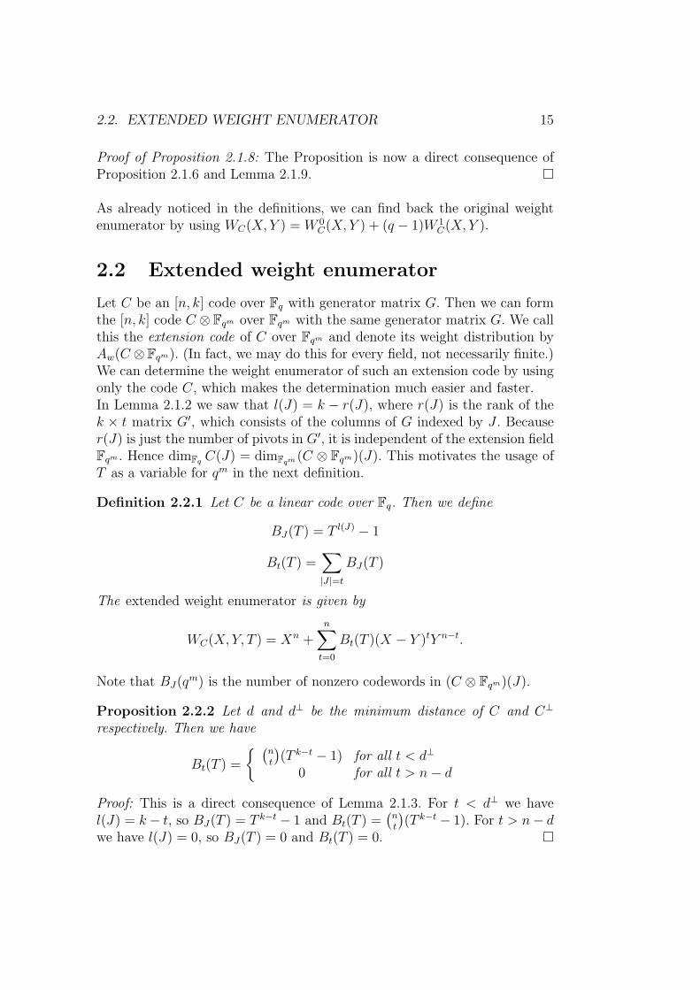
Proof of Proposition 2.1.8: The Proposition is now a direct consequence ofProposition 2.1.6 and Lemma 2.1.9. �
As already noticed in the definitions, we can find back the original weightenumerator by using WC(X, Y ) = W 0
C(X, Y ) + (q − 1)W 1C(X, Y ).
2.2 Extended weight enumerator
Let C be an [n, k] code over Fq with generator matrix G. Then we can formthe [n, k] code C ⊗ Fqm over Fqm with the same generator matrix G. We callthis the extension code of C over Fqm and denote its weight distribution byAw(C ⊗ Fqm). (In fact, we may do this for every field, not necessarily finite.)We can determine the weight enumerator of such an extension code by usingonly the code C, which makes the determination much easier and faster.In Lemma 2.1.2 we saw that l(J) = k − r(J), where r(J) is the rank of thek × t matrix G′, which consists of the columns of G indexed by J . Becauser(J) is just the number of pivots in G′, it is independent of the extension fieldFqm . Hence dimFq C(J) = dimFqm (C ⊗ Fqm)(J). This motivates the usage ofT as a variable for qm in the next definition.
Definition 2.2.1 Let C be a linear code over Fq. Then we define
BJ(T ) = T l(J) − 1
Bt(T ) =∑|J |=t
BJ(T )
The extended weight enumerator is given by
WC(X, Y, T ) = Xn +n∑
t=0
Bt(T )(X − Y )tY n−t.
Note that BJ(qm) is the number of nonzero codewords in (C ⊗ Fqm)(J).
Proposition 2.2.2 Let d and d⊥ be the minimum distance of C and C⊥
respectively. Then we have
Bt(T ) =
{ (nt
)(T k−t − 1) for all t < d⊥
0 for all t > n− d
Proof: This is a direct consequence of Lemma 2.1.3. For t < d⊥ we havel(J) = k− t, so BJ(T ) = T k−t − 1 and Bt(T ) =
(nt
)(T k−t − 1). For t > n− d
we have l(J) = 0, so BJ(T ) = 0 and Bt(T ) = 0. �
16 CHAPTER 2. WEIGHT ENUMERATOR
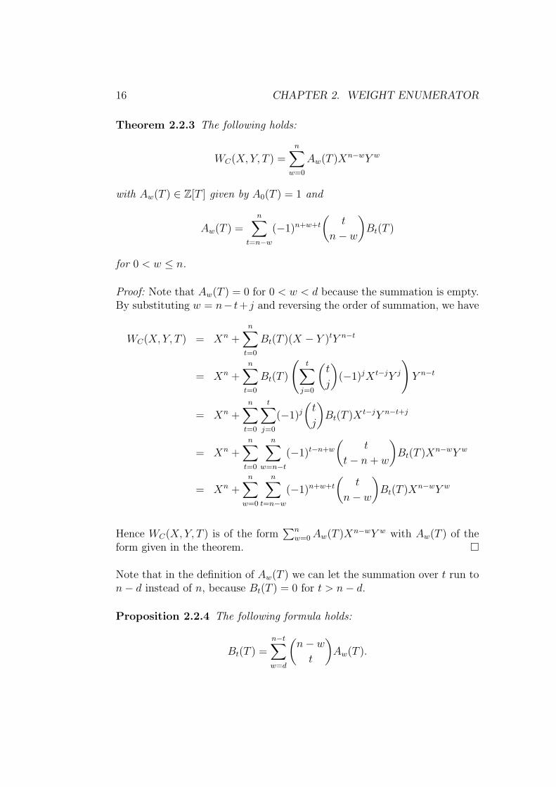
Theorem 2.2.3 The following holds:
WC(X, Y, T ) =n∑
w=0
Aw(T )Xn−wY w
with Aw(T ) ∈ Z[T ] given by A0(T ) = 1 and
Aw(T ) =n∑
t=n−w
(−1)n+w+t
(t
n− w
)Bt(T )
for 0 < w ≤ n.
Proof: Note that Aw(T ) = 0 for 0 < w < d because the summation is empty.By substituting w = n− t+ j and reversing the order of summation, we have
WC(X, Y, T ) = Xn +n∑
t=0
Bt(T )(X − Y )tY n−t
= Xn +n∑
t=0
Bt(T )
(t∑
j=0
(t
j
)(−1)jX t−jY j
)Y n−t
= Xn +n∑
t=0
t∑j=0
(−1)j
(t
j
)Bt(T )X t−jY n−t+j
= Xn +n∑
t=0
n∑w=n−t
(−1)t−n+w
(t
t− n+ w
)Bt(T )Xn−wY w
= Xn +n∑
w=0
n∑t=n−w
(−1)n+w+t
(t
n− w
)Bt(T )Xn−wY w
Hence WC(X, Y, T ) is of the form∑n
w=0Aw(T )Xn−wY w with Aw(T ) of theform given in the theorem. �
Note that in the definition of Aw(T ) we can let the summation over t run ton− d instead of n, because Bt(T ) = 0 for t > n− d.
Proposition 2.2.4 The following formula holds:
Bt(T ) =n−t∑w=d
(n− wt
)Aw(T ).
2.2. EXTENDED WEIGHT ENUMERATOR 17
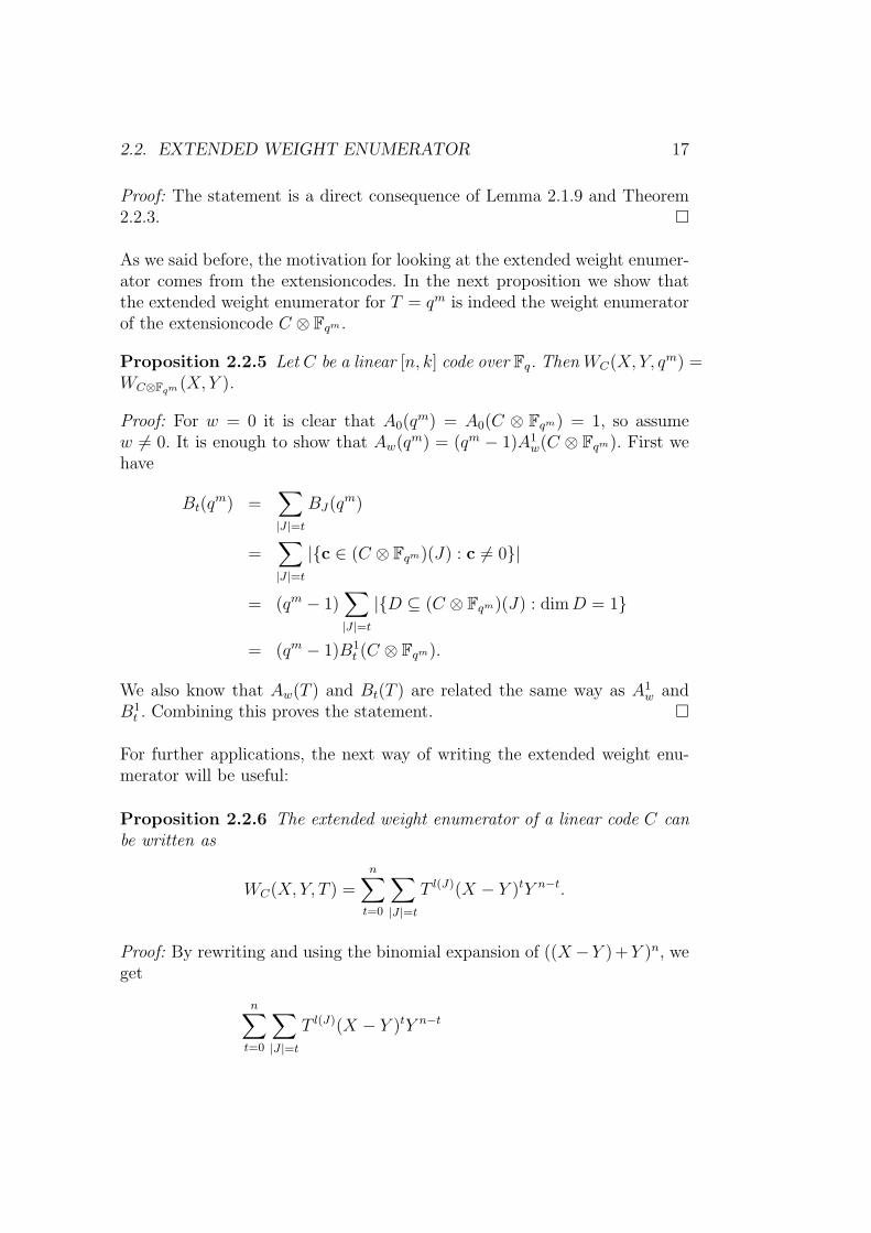
Proof: The statement is a direct consequence of Lemma 2.1.9 and Theorem2.2.3. �
As we said before, the motivation for looking at the extended weight enumer-ator comes from the extensioncodes. In the next proposition we show thatthe extended weight enumerator for T = qm is indeed the weight enumeratorof the extensioncode C ⊗ Fqm .
Proposition 2.2.5 Let C be a linear [n, k] code over Fq. Then WC(X, Y, qm) =WC⊗Fqm (X, Y ).
Proof: For w = 0 it is clear that A0(qm) = A0(C ⊗ Fqm) = 1, so assume
w 6= 0. It is enough to show that Aw(qm) = (qm − 1)A1w(C ⊗ Fqm). First we
have
Bt(qm) =
∑|J |=t
BJ(qm)
=∑|J |=t
|{c ∈ (C ⊗ Fqm)(J) : c 6= 0}|
= (qm − 1)∑|J |=t
|{D ⊆ (C ⊗ Fqm)(J) : dimD = 1}
= (qm − 1)B1t (C ⊗ Fqm).
We also know that Aw(T ) and Bt(T ) are related the same way as A1w and
B1t . Combining this proves the statement. �
For further applications, the next way of writing the extended weight enu-merator will be useful:
Proposition 2.2.6 The extended weight enumerator of a linear code C canbe written as
WC(X, Y, T ) =n∑
t=0
∑|J |=t
T l(J)(X − Y )tY n−t.
Proof: By rewriting and using the binomial expansion of ((X−Y ) +Y )n, weget
n∑t=0
∑|J |=t
T l(J)(X − Y )tY n−t
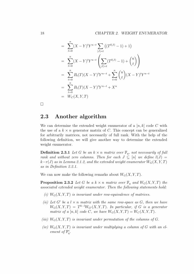
18 CHAPTER 2. WEIGHT ENUMERATOR
=n∑
t=0
(X − Y )tY n−t∑|J |=t
((T l(J) − 1) + 1
)
=n∑
t=0
(X − Y )tY n−t
∑|J |=t
(T l(J) − 1) +
(n
t
)=
n∑t=0
Bt(T )(X − Y )tY n−t +n∑
t=0
(n
t
)(X − Y )tY n−t
=n∑
t=0
Bt(T )(X − Y )tY n−t +Xn
= WC(X, Y, T )
�
2.3 Another algorithm
We can determine the extended weight enumerator of a [n, k] code C withthe use of a k × n generator matrix of C. This concept can be generalizedfor arbitrarily matrices, not necessarily of full rank. With the help of thefollowing definition, we will give another way to determine the extendedweight enumerator.
Definition 2.3.1 Let G be an k × n matrix over Fq, not necessarily of fullrank and without zero columns. Then for each J ⊆ [n] we define l(J) =k−r(J) as in Lemma 2.1.2, and the extended weight enumerator WG(X, Y, T )as in Definition 2.2.1.
We can now make the following remarks about WG(X, Y, T ).
Proposition 2.3.2 Let G be a k × n matrix over Fq and WG(X, Y, T ) theassociated extended weight enumerator. Then the following statements hold:
(i) WG(X, Y, T ) is invariant under row-equivalence of matrices.
(ii) Let G′ be a l × n matrix with the same row-space as G, then we haveWG(X, Y, T ) = T k−lWG′(X, Y, T ). In particular, if G is a generatormatrix of a [n, k] code C, we have WG(X, Y, T ) = WC(X, Y, T ).
(iii) WG(X, Y, T ) is invariant under permutation of the columns of G.
(iv) WG(X, Y, T ) is invariant under multiplying a column of G with an el-ement of F∗q.
2.3. ANOTHER ALGORITHM 19
(v) If G is the direct sum of G1 and G2, i.e. of the form(G1 00 G2
),
then WG(X, Y, T ) = WG1(X, Y, T ) ·WG2(X, Y, T ).
Proof: If we multiply G from the left with an invertible k × k matrix, ther(J) do not change, and therefore (i) holds. For (ii), we may assume withoutloss of generality that k ≥ l. Because G and G′ have the same row-space, ther(J) are the same. Using Proposition 2.2.6 we have for G
WG(X, Y, T ) =n∑
t=0
∑|J |=t
T l(J)(X − Y )tY n−t
=n∑
t=0
∑|J |=t
T k−r(J)(X − Y )tY n−t
= T k−l
n∑t=0
∑|J |=t
T l−r(J)(X − Y )tY n−t
= T k−lWG′(X, Y, T ).
The last part of (ii) and (iii)–(v) follow directly from the definitions. �
With the use of the extended weight enumerator for general matrices, we canderive a recursive algorithm to determine the extended weight enumeratorof a code. If G is a k × n matrix, we denote by G∗ a matrix which is row-equivalent to G and has a column a of the form (1, 0, . . . , 0)T . In general, thisreduction G∗ is not unique.The matrix G∗− a is the k× (n− 1) matrix G∗ with the column a removed,and G∗/a is the (k − 1) × (n − 1) matrix G∗ with the column a and thefirst row removed. For the extended weight enumerators of these matrices,we have the following connection (we omit the (X, Y, T ) part for clarity):
Proposition 2.3.3 For the extended weight enumerator of a reduced matrixG∗ holds
WG∗ = (X − Y )WG∗/a + YWG∗−a
Proof: We distinguish between two cases here. First, assume that G∗−a andG ∗ /a have the same rank. Then we can choose a G∗ with all zeros in thefirst row, except for the 1 in the column a. So G∗ is the direct sum of 1 andG∗/a. By Proposition 2.3.2 parts (v) and (ii) we have
WG∗ = (X + (T − 1)Y )WG∗/a and WG∗−a = TWG∗/a.
20 CHAPTER 2. WEIGHT ENUMERATOR
Combining the two gives
WG∗ = (X + (T − 1)Y )WG∗/a
= (X − Y )WG∗/a + Y TWG∗/a
= (X − Y )WG∗/a + YWG∗−a.
For the second case, assume that G∗ − a and G∗/a do not have the samerank. This implies G∗ and G∗ − a do have the same rank. The vectors in{xG∗ : x ∈ Fqm} now fall into two cases: those which have a zero on positiona, and those which do not. The first have extended weight distribution equalto XWG∗/a(X, Y, qm). The second are the vectors in {x(G∗ − a) : x ∈ Fqm}but not in {x(G∗/a) : x ∈ Fqm}, with a single nonzero coordinate added. Sowe have
WG∗ = XWG∗/a(X, Y, qm) + Y (WG∗−a(X, Y, qm)−WG∗/a(X, Y, qm)).
Changing to T by Lagrange interpolation proves the given formula. �
Theorem 2.3.4 Let G be a k × n matrix over Fq with n > k of the formG∗ = (Ik|P ), where P is a k× (n− k) matrix over Fq. Let A ⊆ [k] and writePA for the matrix formed by the rows of P indexed by A. Let WA(X, Y, T ) =WPA
(X, Y, T ). Then the following holds:
WC(X, Y, T ) =k∑
l=0
∑|A|=l
Y l(X − Y )k−lWA(X, Y, T ).
Proof: We use the formula of the last proposition recursively. We denote theconstruction of G∗−a by G1 and the construction of G∗/a by G2. Repeatingthis procedure, we get the matrices G11, G12, G21 and G22. So we get for theweight enumerator
WG = Y 2WG11 + Y (X − Y )WG12 + Y (X − Y )WG21 + (X − Y )2WG22 .
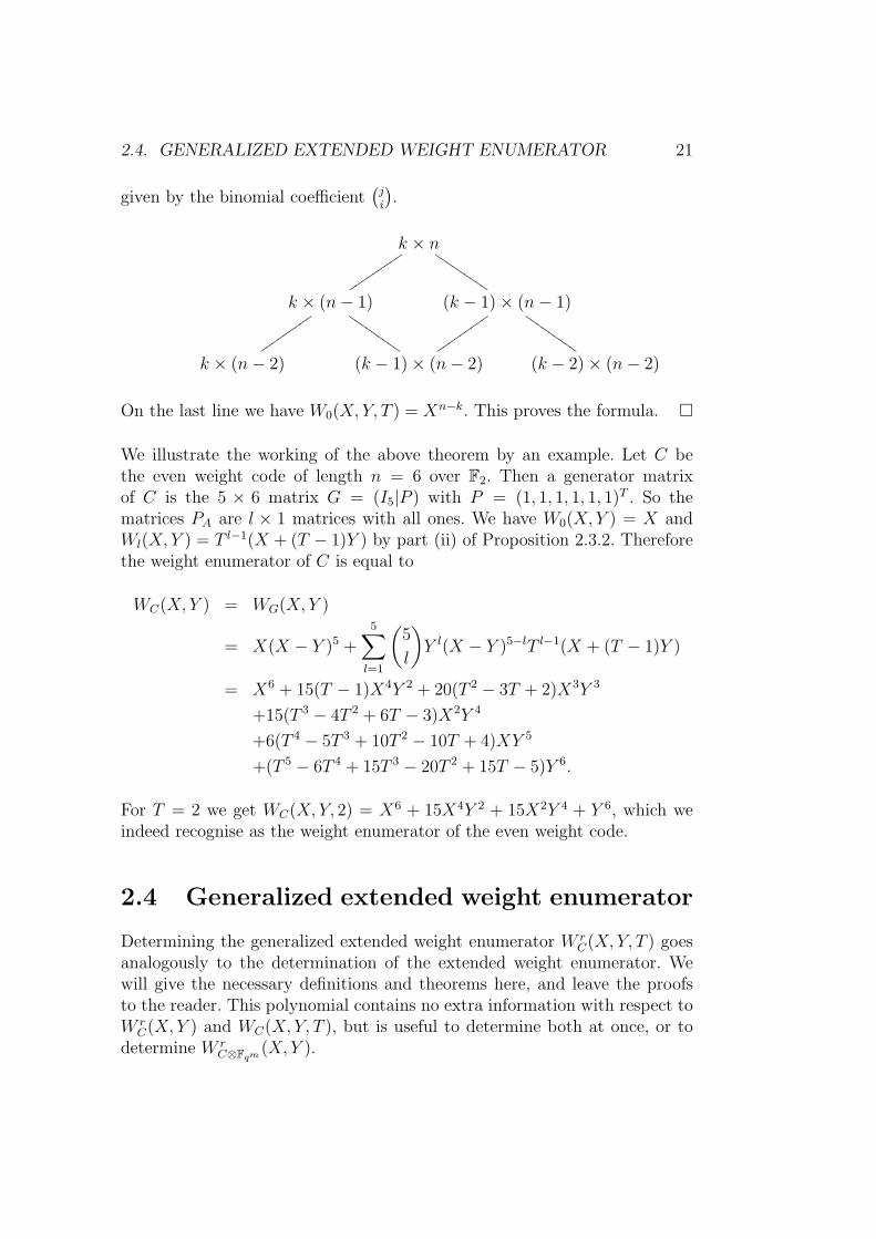
Repeating this procedure k times, we get 2k matrices with n − k columnsand 0, . . . , k rows, which form exactly the PA. In the diagram are the sizesof the matrices of the first two steps: note that only the k× n matrix on tophas to be of full rank. The number of matrices of size (k − i) × (n − j) are
2.4. GENERALIZED EXTENDED WEIGHT ENUMERATOR 21
given by the binomial coefficient(
ji
).
k × n
uuuuuuuuu
IIIIIIIII
k × (n− 1)
uuuuuuuuu
IIIIIIIII(k − 1)× (n− 1)
uuuuuuuuu
IIIIIIIII
k × (n− 2) (k − 1)× (n− 2) (k − 2)× (n− 2)
On the last line we have W0(X, Y, T ) = Xn−k. This proves the formula. �
We illustrate the working of the above theorem by an example. Let C bethe even weight code of length n = 6 over F2. Then a generator matrixof C is the 5 × 6 matrix G = (I5|P ) with P = (1, 1, 1, 1, 1, 1)T . So thematrices PA are l × 1 matrices with all ones. We have W0(X, Y ) = X andWl(X, Y ) = T l−1(X + (T − 1)Y ) by part (ii) of Proposition 2.3.2. Thereforethe weight enumerator of C is equal to
WC(X, Y ) = WG(X, Y )
= X(X − Y )5 +5∑
l=1
(5
l
)Y l(X − Y )5−lT l−1(X + (T − 1)Y )
= X6 + 15(T − 1)X4Y 2 + 20(T 2 − 3T + 2)X3Y 3
+15(T 3 − 4T 2 + 6T − 3)X2Y 4
+6(T 4 − 5T 3 + 10T 2 − 10T + 4)XY 5
+(T 5 − 6T 4 + 15T 3 − 20T 2 + 15T − 5)Y 6.
For T = 2 we get WC(X, Y, 2) = X6 + 15X4Y 2 + 15X2Y 4 + Y 6, which weindeed recognise as the weight enumerator of the even weight code.
2.4 Generalized extended weight enumerator
Determining the generalized extended weight enumerator W rC(X, Y, T ) goes
analogously to the determination of the extended weight enumerator. Wewill give the necessary definitions and theorems here, and leave the proofsto the reader. This polynomial contains no extra information with respect toW r
C(X, Y ) and WC(X, Y, T ), but is useful to determine both at once, or todetermine W r
C⊗Fqm (X, Y ).
22 CHAPTER 2. WEIGHT ENUMERATOR
Definition 2.4.1 Let C be a linear code over Fq. Then we define
BrJ(T ) =
[l(J)
r
]T
Brt (T ) =
∑|J |=t
BrJ(T )
The generalized extended weight enumerator is given by
W rC(X, Y, T ) =
n∑t=0
Brt (T )(X − Y )tY n−t.
Proposition 2.4.2 Let d and d⊥ be the minimum distance of C and C⊥
respectively. Then we have
Brt (T ) =
{ (nt
) [k−tr
]T
for all t < d⊥
0 for all t > n− dr
Theorem 2.4.3 The following holds:
W rC(X, Y, T ) =
n∑w=0
Arw(T )Xn−wY w
with Arw(T ) ∈ Z[T ] given by Ar
0(T ) = δ0r and
Arw(T ) =
n∑t=n−w
(−1)n+w+t
(t
n− w
)Br
t (T )
for 0 < w ≤ n.
Proposition 2.4.4 The following formula holds:
Brt (T ) =
n−t∑w=dr
(n− wt
)Ar
w(T ).
Proposition 2.4.5 Let C be a linear [n, k] code over Fq. Then we haveW r
C(X, Y, qm) = W rC⊗Fqm (X, Y ).
Proof: For w = 0 it is clear that Ar0(q
m) = Ar0(C ⊗ Fqm), so assume w 6= 0.
It is enough to show that Arw(qm) = Ar
w(C ⊗ Fqm). Let V be a linear vectorspace over Fqm with dimV = l(J), then we have
BrJ(qm) = |{U ⊆ V : dimU = r}|
= |{D ⊆ (C ⊗ Fqm)(J) : dimD = r}= Br
J(C ⊗ Fqm).
This implies that Brt (qm) = Br
t (C ⊗ Fqm). We also know that Arw(T ) and
Brt (T ) are related the same way as Ar
w and Brt . Combining this proves the
statement. �
2.5. NOTES 23
2.5 Notes
The determination of the generalized and extended weight enumerator is ageneralisation of the method used by Pellikaan, Wu and Bulygin [10]. Lemma2.1.9 and many other binomial identities can be found in Riordan [11]. Notealso the similarity with Simonis [12]: for example, Lemma 2.1.2 is similarwith proposition (i) from this article. The form
∑nt=0Bt(X−Y )tY n−t for the
weight enumerator was first introduced in [5] and later in [13]. In the nextchapters we will see more advantages of using this description of the weightenumerator.The algorithm in section 2.3 is new material, and based on Tutte-Grothendieckdecomposition of matrices. Greene [4] first used this decomposition for thedetermination of the weight enumerator. Proposition 2.3.3 is a generalizationof his proposition 4.3.
24 CHAPTER 2. WEIGHT ENUMERATOR
Chapter 3
Connections
3.1 Extended in terms of generalized
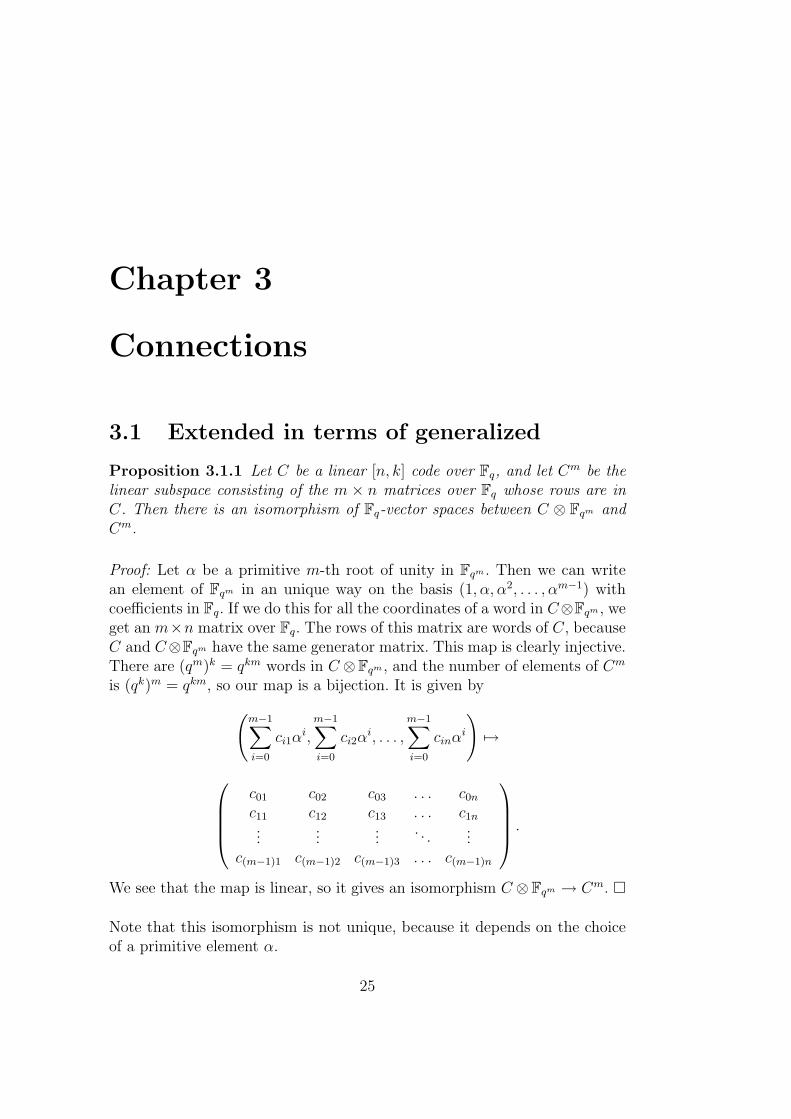
Proposition 3.1.1 Let C be a linear [n, k] code over Fq, and let Cm be thelinear subspace consisting of the m × n matrices over Fq whose rows are inC. Then there is an isomorphism of Fq-vector spaces between C ⊗ Fqm andCm.
Proof: Let α be a primitive m-th root of unity in Fqm . Then we can writean element of Fqm in an unique way on the basis (1, α, α2, . . . , αm−1) withcoefficients in Fq. If we do this for all the coordinates of a word in C⊗Fqm , weget an m×n matrix over Fq. The rows of this matrix are words of C, becauseC and C⊗Fqm have the same generator matrix. This map is clearly injective.There are (qm)k = qkm words in C ⊗Fqm , and the number of elements of Cm
is (qk)m = qkm, so our map is a bijection. It is given by(m−1∑i=0
ci1αi,
m−1∑i=0
ci2αi, . . . ,
m−1∑i=0
cinαi
)7→
c01 c02 c03 . . . c0n
c11 c12 c13 . . . c1n...
......
. . ....
c(m−1)1 c(m−1)2 c(m−1)3 . . . c(m−1)n
.
We see that the map is linear, so it gives an isomorphism C ⊗Fqm → Cm. �
Note that this isomorphism is not unique, because it depends on the choiceof a primitive element α.
25
26 CHAPTER 3. CONNECTIONS
Lemma 3.1.2 Let c ∈ C⊗Fqm and M ∈ Cm the corresponding m×n matrixunder a given isomorphism. Let D ⊆ C the subcode generated by M . Thenwt(c) = wt(D).
Proof: If the j-th coordinate cj of c is zero, then the j-th column of M consistsof only zero’s, because the representation of cj on the basis (1, α, α2, . . . , αm−1)is unique. On the other hand, if the j-th column of M consists of all zeros,then cj is also zero. Therefore wt(c) = wt(D). �
Proposition 3.1.3 Let C be a linear code over Fq. Then the weight numera-tor of an extension code and the generalized weight enumerators are connectedvia
Aw(qm) =m∑
r=0
[m, r]qArw.
Proof: We count the number of words in C ⊗ Fqm of weight w in two ways,using the bijection of proposition 3.1.1. The first way is just Aw(T = qm), theleft side of the equation. For the second way, note that every M ∈ Cm gener-ates a subcode of C whose weight is equal to the weight of the correspondingword in C⊗Fqm . Fix this weight w and a dimension r: there are Ar
w subcodesof C of dimension r and weight w. Every such subcode is generated by anr × n matrix whose rows are words of C. Left multiplication by an m × rmatrix of rank r gives an element of Cm which generates the same subcode ofC, and all such elements of Cm are obtained this way. The number of m× rmatrices of rank r is [m, r]q, so summation over all dimensions r gives
Aw(qm) =k∑
r=0
[m, r]qArw.
We can let the summation run to m, because Arw = 0 for r > k and [m, r]q = 0
for r > m. This proves the given formula. �
In general, we have the following theorem.
Theorem 3.1.4 Let C be a linear code over Fq. Then the extended weightnumerator and the generalized weight enumerator are connected via
WC(X, Y, T ) =k∑
r=0
(r−1∏j=0
(T − qj)
)W r
C(X, Y ).
3.2. GENERALIZED IN TERMS OF EXTENDED 27
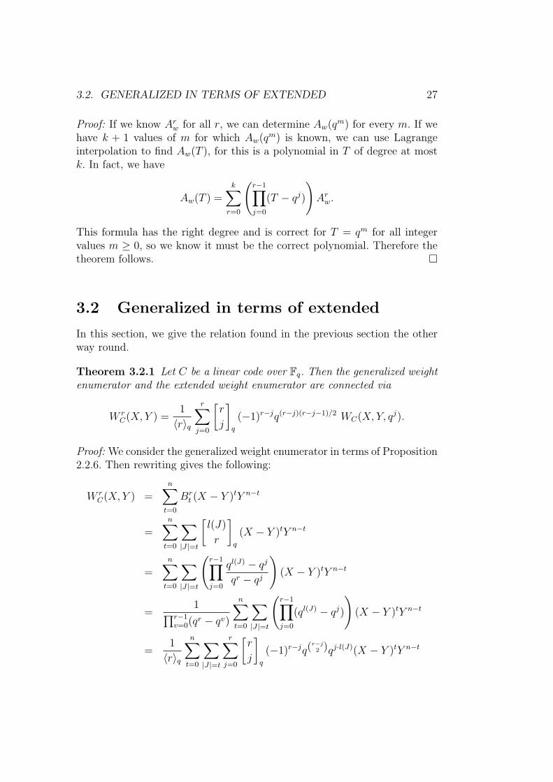
Proof: If we know Arw for all r, we can determine Aw(qm) for every m. If we
have k + 1 values of m for which Aw(qm) is known, we can use Lagrangeinterpolation to find Aw(T ), for this is a polynomial in T of degree at mostk. In fact, we have
Aw(T ) =k∑
r=0
(r−1∏j=0
(T − qj)
)Ar
w.
This formula has the right degree and is correct for T = qm for all integervalues m ≥ 0, so we know it must be the correct polynomial. Therefore thetheorem follows. �
3.2 Generalized in terms of extended
In this section, we give the relation found in the previous section the otherway round.
Theorem 3.2.1 Let C be a linear code over Fq. Then the generalized weightenumerator and the extended weight enumerator are connected via
W rC(X, Y ) =
1
〈r〉q
r∑j=0
[r
j
]q
(−1)r−jq(r−j)(r−j−1)/2 WC(X, Y, qj).
Proof: We consider the generalized weight enumerator in terms of Proposition2.2.6. Then rewriting gives the following:
W rC(X, Y ) =
n∑t=0
Brt (X − Y )tY n−t
=n∑
t=0
∑|J |=t
[l(J)
r
]q
(X − Y )tY n−t
=n∑
t=0
∑|J |=t
(r−1∏j=0
ql(J) − qj
qr − qj
)(X − Y )tY n−t
=1∏r−1
v=0(qr − qv)
n∑t=0
∑|J |=t
(r−1∏j=0
(ql(J) − qj)
)(X − Y )tY n−t
=1
〈r〉q
n∑t=0
∑|J |=t
r∑j=0
[r
j
]q
(−1)r−jq(r−j2 )qj·l(J)(X − Y )tY n−t
28 CHAPTER 3. CONNECTIONS
=1
〈r〉q
r∑j=0
[r
j
]q
(−1)r−jq(r−j2 )
n∑t=0
∑|J |=t
(qj)l(J)(X − Y )tY n−t
=1
〈r〉q
r∑j=0
[r
j
]q
(−1)r−jq(r−j)(r−j−1)/2 WC(X, Y, qj)
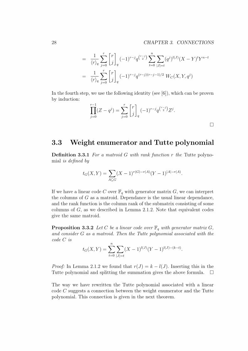
In the fourth step, we use the following identity (see [6]), which can be provenby induction:
r−1∏j=0
(Z − qj) =r∑
j=0
[r
j
]q
(−1)r−jq(r−j2 )Zj.
�
3.3 Weight enumerator and Tutte polynomial
Definition 3.3.1 For a matroid G with rank function r the Tutte polyno-mial is defined by
tG(X, Y ) =∑A⊆G
(X − 1)r(G)−r(A)(Y − 1)|A|−r(A).
If we have a linear code C over Fq with generator matrix G, we can interpretthe columns of G as a matroid. Dependance is the usual linear dependance,and the rank function is the column rank of the submatrix consisting of somecolumns of G, as we described in Lemma 2.1.2. Note that equivalent codesgive the same matroid.
Proposition 3.3.2 Let C be a linear code over Fq with generator matrix G,and consider G as a matroid. Then the Tutte polynomial associated with thecode C is
tG(X, Y ) =n∑
t=0
∑|J |=t
(X − 1)l(J)(Y − 1)l(J)−(k−t).
Proof: In Lemma 2.1.2 we found that r(J) = k − l(J). Inserting this in theTutte polynomial and splitting the summation gives the above formula. �
The way we have rewritten the Tutte polynomial associated with a linearcode C suggests a connection between the weight enumerator and the Tuttepolynomial. This connection is given in the next theorem.
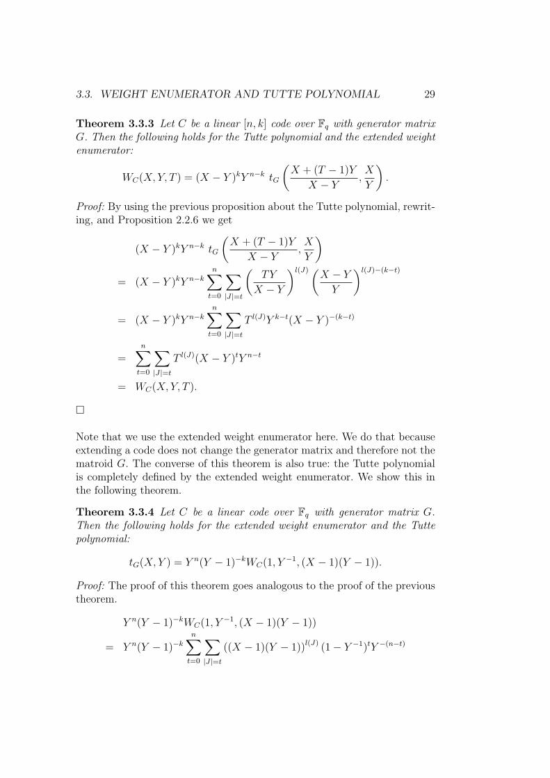
3.3. WEIGHT ENUMERATOR AND TUTTE POLYNOMIAL 29
Theorem 3.3.3 Let C be a linear [n, k] code over Fq with generator matrixG. Then the following holds for the Tutte polynomial and the extended weightenumerator:
WC(X, Y, T ) = (X − Y )kY n−k tG
(X + (T − 1)Y
X − Y,X
Y
).
Proof: By using the previous proposition about the Tutte polynomial, rewrit-ing, and Proposition 2.2.6 we get
(X − Y )kY n−k tG
(X + (T − 1)Y
X − Y,X
Y
)= (X − Y )kY n−k
n∑t=0
∑|J |=t
(TY
X − Y
)l(J)(X − YY
)l(J)−(k−t)
= (X − Y )kY n−k
n∑t=0
∑|J |=t
T l(J)Y k−t(X − Y )−(k−t)
=n∑
t=0
∑|J |=t
T l(J)(X − Y )tY n−t
= WC(X, Y, T ).
�
Note that we use the extended weight enumerator here. We do that becauseextending a code does not change the generator matrix and therefore not thematroid G. The converse of this theorem is also true: the Tutte polynomialis completely defined by the extended weight enumerator. We show this inthe following theorem.
Theorem 3.3.4 Let C be a linear code over Fq with generator matrix G.Then the following holds for the extended weight enumerator and the Tuttepolynomial:
tG(X, Y ) = Y n(Y − 1)−kWC(1, Y −1, (X − 1)(Y − 1)).
Proof: The proof of this theorem goes analogous to the proof of the previoustheorem.
Y n(Y − 1)−kWC(1, Y −1, (X − 1)(Y − 1))
= Y n(Y − 1)−k
n∑t=0
∑|J |=t
((X − 1)(Y − 1))l(J) (1− Y −1)tY −(n−t)
30 CHAPTER 3. CONNECTIONS
=n∑
t=0
∑|J |=t
(X − 1)l(J)(Y − 1)l(J)Y −t(Y − 1)tY −(n−k)Y n(Y − 1)−k
=n∑
t=0
∑|J |=t
(X − 1)l(J)(Y − 1)l(J)−(k−t)
= tG(X, Y ).
�
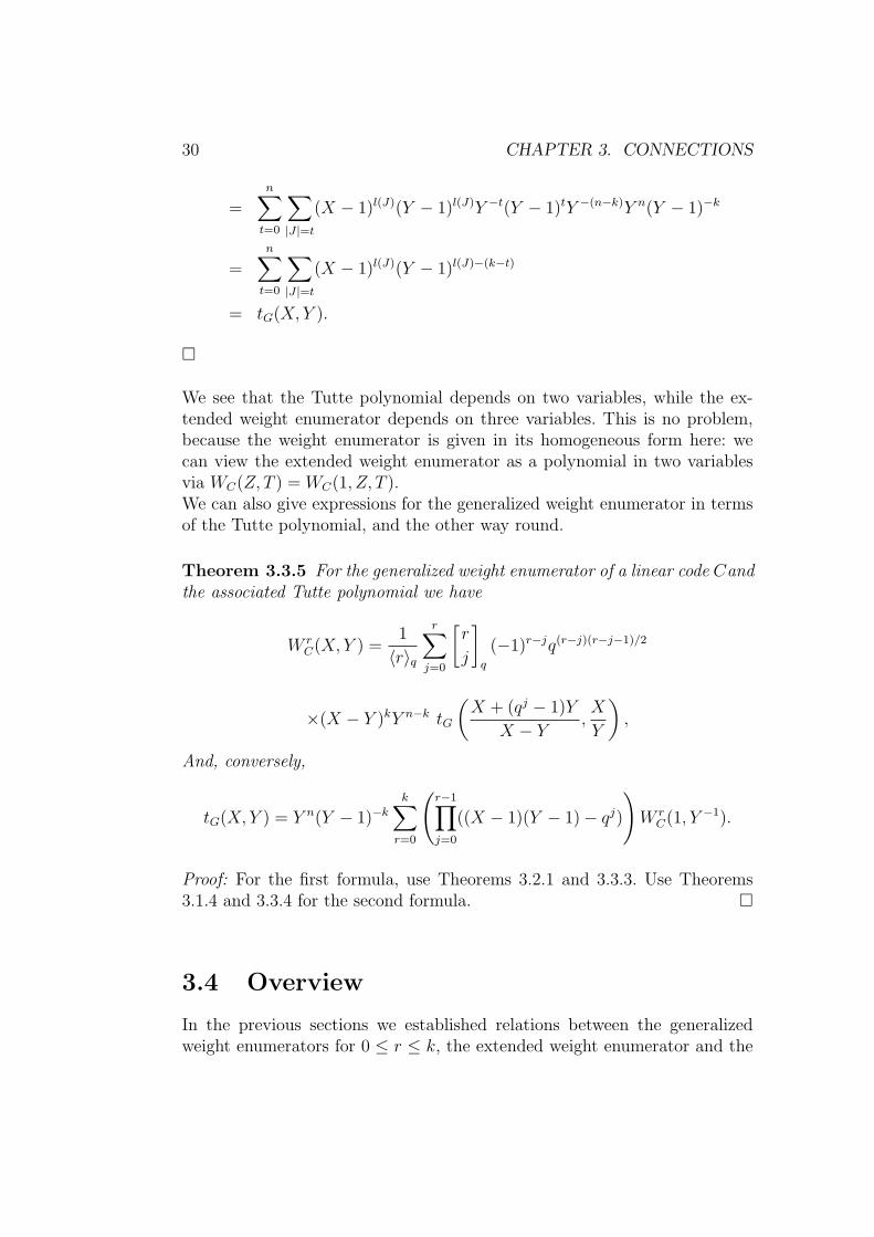
We see that the Tutte polynomial depends on two variables, while the ex-tended weight enumerator depends on three variables. This is no problem,because the weight enumerator is given in its homogeneous form here: wecan view the extended weight enumerator as a polynomial in two variablesvia WC(Z, T ) = WC(1, Z, T ).We can also give expressions for the generalized weight enumerator in termsof the Tutte polynomial, and the other way round.
Theorem 3.3.5 For the generalized weight enumerator of a linear code Candthe associated Tutte polynomial we have
W rC(X, Y ) =
1
〈r〉q
r∑j=0
[r
j
]q
(−1)r−jq(r−j)(r−j−1)/2
×(X − Y )kY n−k tG
(X + (qj − 1)Y
X − Y,X
Y
),
And, conversely,
tG(X, Y ) = Y n(Y − 1)−k
k∑r=0
(r−1∏j=0
((X − 1)(Y − 1)− qj)
)W r
C(1, Y −1).
Proof: For the first formula, use Theorems 3.2.1 and 3.3.3. Use Theorems3.1.4 and 3.3.4 for the second formula. �
3.4 Overview
In the previous sections we established relations between the generalizedweight enumerators for 0 ≤ r ≤ k, the extended weight enumerator and the
3.5. NOTES 31
Tutte polynomial. We summarize this in the following diagram:
WC(X, Y )
WC(X, Y, T )
3.2.1yy
3.3.4��
mm
{W rC(X, Y )}kr=0
3.1.4 44
3.3.5 //
\\
tG(X, Y )3.3.5
oo
3.3.3
OO
{W rC(X, Y, T )}kr=0
--
kk
��
dd
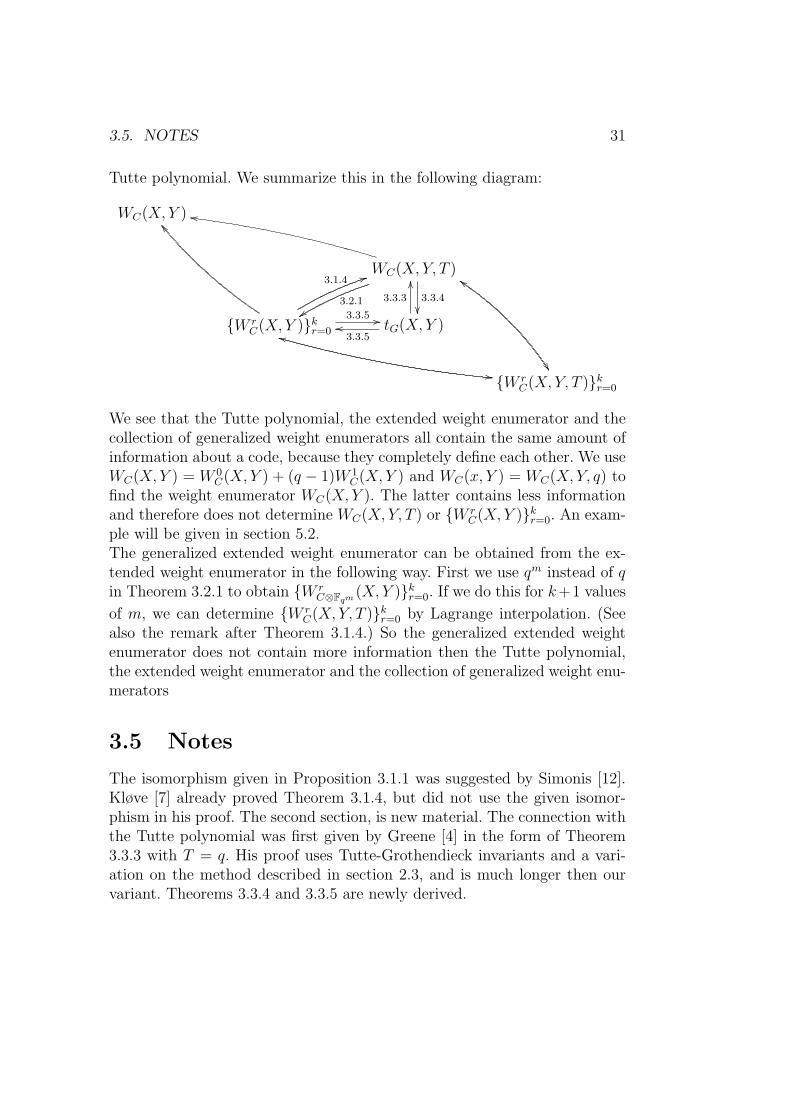
We see that the Tutte polynomial, the extended weight enumerator and thecollection of generalized weight enumerators all contain the same amount ofinformation about a code, because they completely define each other. We useWC(X, Y ) = W 0
C(X, Y ) + (q − 1)W 1C(X, Y ) and WC(x, Y ) = WC(X, Y, q) to
find the weight enumerator WC(X, Y ). The latter contains less informationand therefore does not determine WC(X, Y, T ) or {W r
C(X, Y )}kr=0. An exam-ple will be given in section 5.2.The generalized extended weight enumerator can be obtained from the ex-tended weight enumerator in the following way. First we use qm instead of qin Theorem 3.2.1 to obtain {W r
C⊗Fqm (X, Y )}kr=0. If we do this for k+1 values
of m, we can determine {W rC(X, Y, T )}kr=0 by Lagrange interpolation. (See
also the remark after Theorem 3.1.4.) So the generalized extended weightenumerator does not contain more information then the Tutte polynomial,the extended weight enumerator and the collection of generalized weight enu-merators
3.5 Notes
The isomorphism given in Proposition 3.1.1 was suggested by Simonis [12].Kløve [7] already proved Theorem 3.1.4, but did not use the given isomor-phism in his proof. The second section, is new material. The connection withthe Tutte polynomial was first given by Greene [4] in the form of Theorem3.3.3 with T = q. His proof uses Tutte-Grothendieck invariants and a vari-ation on the method described in section 2.3, and is much longer then ourvariant. Theorems 3.3.4 and 3.3.5 are newly derived.

32 CHAPTER 3. CONNECTIONS
Chapter 4
MacWilliams identities
4.1 Using the Tutte polynomial
In this section, we will prove the MacWilliams identities using the Tuttepolynomial. We do this because of the following very useful relation betweenthe Tutte polynomial of a matroid and its dual:
Theorem 4.1.1 Let tG(X, Y ) be the Tutte polynomial of a matroid G, andlet G∗ be the dual matroid. Then tG(X, Y ) = tG∗(Y,X).
Proof (sketch): To prove the theorem, we use two relations between the rankfunction of a matroid G and its dual G∗ with underlying set S:
r∗(G∗) + r(G) = |S|, r∗(A) = |A|+ r(S − A)− r(G).
This relations can be proved using basic facts about matroids. Substitutingthe last relation into the definition of the Tutte polynomial for the dual code,gives
tG∗(X, Y ) =∑
A⊆G∗
(X − 1)r∗(G∗)−r∗(A)(Y − 1)|A|−r∗(A)
=∑A⊆G
(X − 1)r∗(G∗)−|A|−r(S−A)+r(G)(Y − 1)r(G)−r(S−A)
=∑A⊆G
(X − 1)|S−A|−r(S−A)(Y − 1)r(G)−r(S−A)
= tG(Y,X)
In the last step, we use that the summation over all A ⊆ G is the same as asummation over all S − A ⊆ G. This proves the theorem. �
33
34 CHAPTER 4. MACWILLIAMS IDENTITIES
If we consider a code as a matroid, then the dual matroid is the dual code.Therefore we can use the above theorem to prove the MacWilliams relations.
Theorem 4.1.2 (MacWilliams) Let C be a code and let C⊥ be its dual.Then the extended weight enumerator of C completely determines the ex-tended weight enumerator of C⊥ and vice versa, via the following formula:
WC⊥(X, Y, T ) = T−kWC(X + (T − 1)Y,X − Y, T ).
Proof: Using the previous theorem, and the relation between the weight enu-merator and the Tutte polynomial, we find
T−kWC(X + (T − 1)Y,X − Y, T )
= T−k(TY )k(X − Y )n−k tG
(X
Y,X + (T − 1)Y
X − Y
)= Y k(X − Y )n−k tG
(X + (T − 1)Y
X − Y,X
Y
)= WC⊥(X, Y, T ).
Notice in the last step that dimC⊥ = n− k, and n− (n− k) = k. �
4.2 Generalized MacWilliams identities
We can use the relations in Theorems 3.1.4 and 3.2.1 to prove the MacWilliamsidentities for the generalized weight enumerator.
Theorem 4.2.1 Let C be a code and let C⊥ be its dual. Then the gener-alized weight enumerators of C completely determine the generalized weightenumerators of C⊥ and vice versa, via the following formula:
W rC⊥(X, Y ) =
r∑j=0
j∑l=0
(−1)r−j q(r−j)(r−j−1)/2−j(r−j)−l(j−l)−jk
〈r − j〉q〈j − l〉qW l
C(X + (qj − 1)Y,X − Y ).
Proof: We write the generalized weight enumerator in terms of the extendedweight enumerator, use the MacWilliams identities for the extended weight
4.3. AN ALTERNATIVE APPROACH 35
enumerator, and convert back to the generalized weight enumerator.
W rC⊥ =
1
〈r〉q
r∑j=0
[r
j
]q
(−1)r−jq(r−j)(r−j−1)/2 WC⊥(X, Y, qi)
=r∑
j=0
(−1)r−j q(r−j)(r−j−1)/2−j(r−j)
〈j〉q〈r − j〉qq−jkWc(X + (qj − 1)Y,X − Y, qj)
=r∑
j=0
(−1)r−j q(r−j)(r−j−1)/2−j(r−j)−jk
〈j〉q〈r − j〉q
×j∑
l=0
〈j〉qql(j−l)〈j − l〉q
W lC(X + (qj − 1, X − Y )
=r∑
j=0
j∑l=0
(−1)r−j q(r−j)(r−j−1)/2−j(r−j)−l(j−l)−jk
〈r − j〉q〈j − l〉q
×W lC(X + (qj − 1, X − Y ).
�
4.3 An alternative approach
In [12] Simonis proved an alternative version of the generalized MacWilliamsidentities. We will prove this theorem directly, by showing the equivalencewith Theorem 4.2.1.
Theorem 4.3.1 The generalized Hamming weights Arw of a linear [n, k] code
C over Fq and the generalized Hamming weights Arw of the dual code C⊥ are
related via
n∑i=0
(n− in−m
)Ar
i =r∑
l=0
ql(m−k+l−r)
[m− kr − l
]q
n∑v=0
(n− vm
)Al
v.
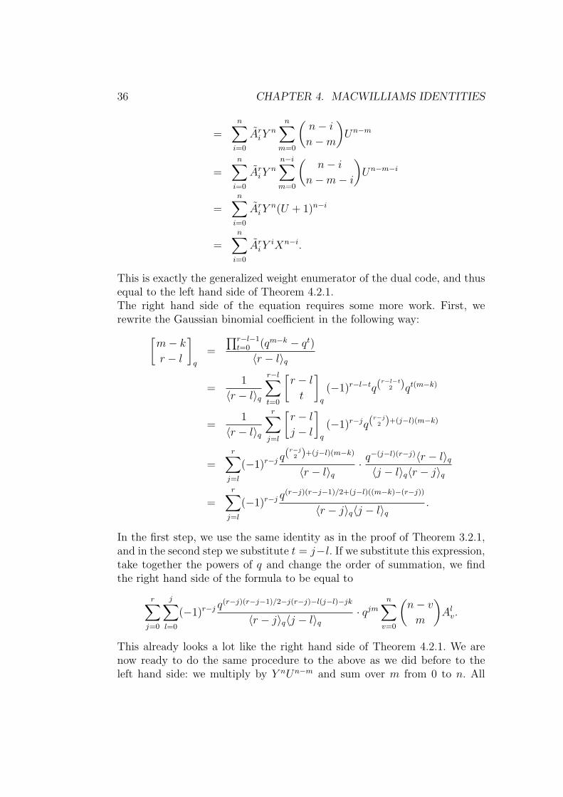
Proof: We will multiply both sides of the equation by Y nUn−m and sum overm from 0 to n. We start with the left hand side of the equation. Changing theorder of summation, using the binomial expansion of (U+1)n−i and changingvariables via X = Y (U + 1) gives
n∑m=0
Y nUn−m
n∑i=0
(n− in−m
)Ar
i
36 CHAPTER 4. MACWILLIAMS IDENTITIES
=n∑
i=0
AriY
n
n∑m=0
(n− in−m
)Un−m
=n∑
i=0
AriY
n
n−i∑m=0
(n− i
n−m− i
)Un−m−i
=n∑
i=0
AriY
n(U + 1)n−i
=n∑
i=0
AriY
iXn−i.
This is exactly the generalized weight enumerator of the dual code, and thusequal to the left hand side of Theorem 4.2.1.The right hand side of the equation requires some more work. First, werewrite the Gaussian binomial coefficient in the following way:[
m− kr − l
]q
=
∏r−l−1t=0 (qm−k − qt)
〈r − l〉q
=1
〈r − l〉q
r−l∑t=0
[r − lt
]q
(−1)r−l−tq(r−l−t
2 )qt(m−k)
=1
〈r − l〉q
r∑j=l
[r − lj − l
]q
(−1)r−jq(r−j2 )+(j−l)(m−k)
=r∑
j=l
(−1)r−j q(r−j
2 )+(j−l)(m−k)
〈r − l〉q· q−(j−l)(r−j)〈r − l〉q〈j − l〉q〈r − j〉q
=r∑
j=l
(−1)r−j q(r−j)(r−j−1)/2+(j−l)((m−k)−(r−j))
〈r − j〉q〈j − l〉q.
In the first step, we use the same identity as in the proof of Theorem 3.2.1,and in the second step we substitute t = j−l. If we substitute this expression,take together the powers of q and change the order of summation, we findthe right hand side of the formula to be equal to
r∑j=0
j∑l=0
(−1)r−j q(r−j)(r−j−1)/2−j(r−j)−l(j−l)−jk
〈r − j〉q〈j − l〉q· qjm
n∑v=0
(n− vm
)Al
v.
This already looks a lot like the right hand side of Theorem 4.2.1. We arenow ready to do the same procedure to the above as we did before to theleft hand side: we multiply by Y nUn−m and sum over m from 0 to n. All
4.3. AN ALTERNATIVE APPROACH 37
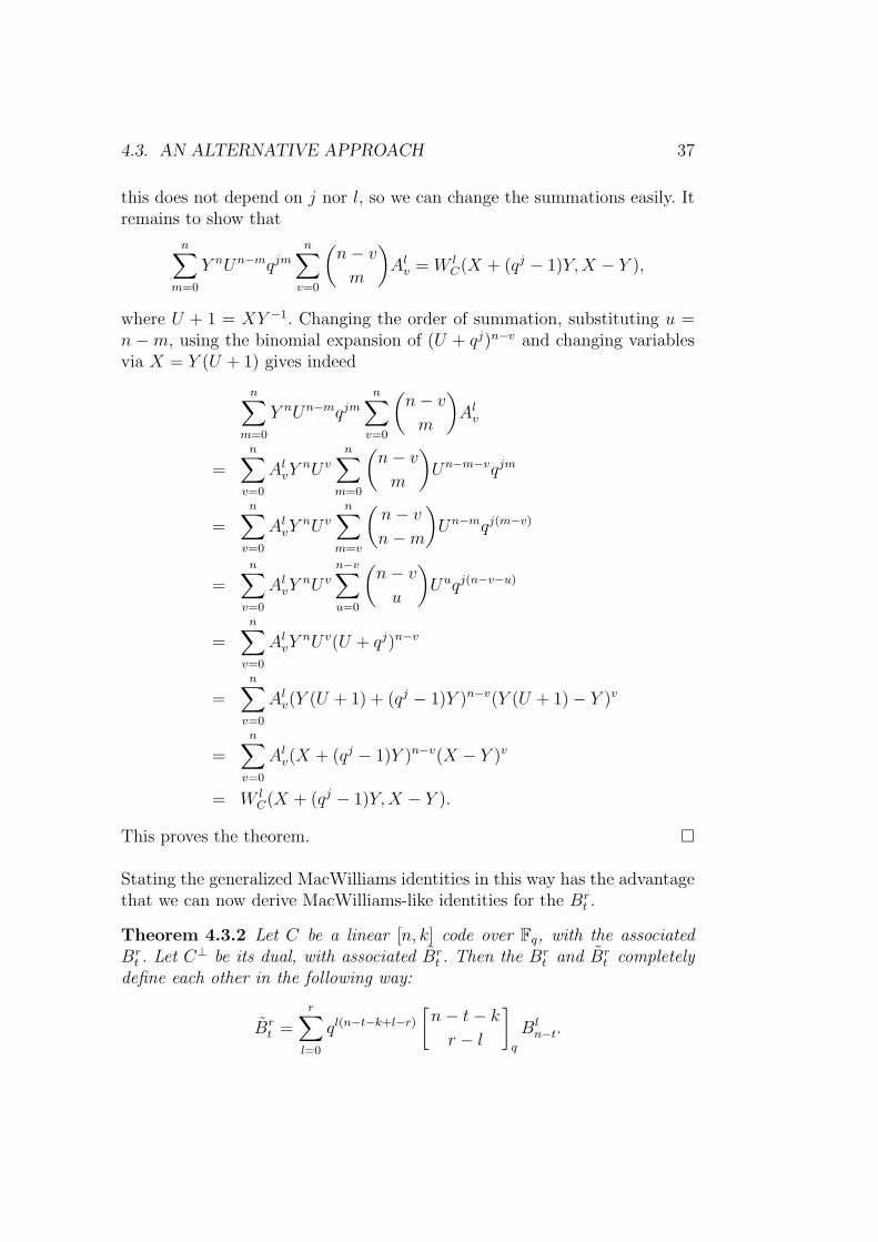
this does not depend on j nor l, so we can change the summations easily. Itremains to show that
n∑m=0
Y nUn−mqjm
n∑v=0
(n− vm
)Al
v = W lC(X + (qj − 1)Y,X − Y ),
where U + 1 = XY −1. Changing the order of summation, substituting u =n −m, using the binomial expansion of (U + qj)n−v and changing variablesvia X = Y (U + 1) gives indeed
n∑m=0
Y nUn−mqjm
n∑v=0
(n− vm
)Al
v
=n∑
v=0
AlvY
nU v
n∑m=0
(n− vm
)Un−m−vqjm
=n∑
v=0
AlvY
nU v
n∑m=v
(n− vn−m
)Un−mqj(m−v)
=n∑
v=0
AlvY
nU v
n−v∑u=0
(n− vu
)Uuqj(n−v−u)
=n∑
v=0
AlvY
nU v(U + qj)n−v
=n∑
v=0
Alv(Y (U + 1) + (qj − 1)Y )n−v(Y (U + 1)− Y )v
=n∑
v=0
Alv(X + (qj − 1)Y )n−v(X − Y )v
= W lC(X + (qj − 1)Y,X − Y ).
This proves the theorem. �
Stating the generalized MacWilliams identities in this way has the advantagethat we can now derive MacWilliams-like identities for the Br
t .
Theorem 4.3.2 Let C be a linear [n, k] code over Fq, with the associatedBr
t . Let C⊥ be its dual, with associated Brt . Then the Br
t and Brt completely
define each other in the following way:
Brt =
r∑l=0
ql(n−t−k+l−r)
[n− t− kr − l
]q
Bln−t.
38 CHAPTER 4. MACWILLIAMS IDENTITIES
Proof: The formula is a direct consequence of the previous theorem andProposition 2.1.6, with n−m replaced by t. �
As we see, this formula is much more pleasant then the one in Theorems4.2.1 and 4.3.1. This motivates the use of the Br
t for the weight enumerator.
4.4 Notes
Greene [4] first used the Tutte polynomial to prove the MacWilliams identi-ties, see also Brylawsky and Oxley [2]. Theorem 4.2.1 was proved by Kløvein [7], although he uses only half of the relations between the generalizedweight enumerator and the extended weight enumerator. Using both makesthe proof much shorter. The formula in Theorem 4.3.1 was proved by Simonisin [12] with use of an idea quite similar to the Br
t we use. The connectionbetween the two formulas is first proven here, and uses an argument similarto Blahut’s proof [1] of the ordinary MacWilliams relations.
Chapter 5
Examples
5.1 MDS codes
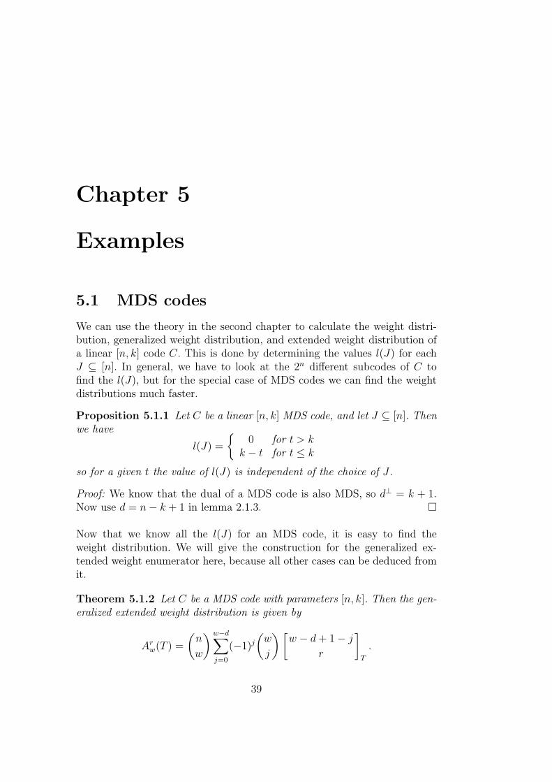
We can use the theory in the second chapter to calculate the weight distri-bution, generalized weight distribution, and extended weight distribution ofa linear [n, k] code C. This is done by determining the values l(J) for eachJ ⊆ [n]. In general, we have to look at the 2n different subcodes of C tofind the l(J), but for the special case of MDS codes we can find the weightdistributions much faster.
Proposition 5.1.1 Let C be a linear [n, k] MDS code, and let J ⊆ [n]. Thenwe have
l(J) =
{0 for t > k
k − t for t ≤ k
so for a given t the value of l(J) is independent of the choice of J .
Proof: We know that the dual of a MDS code is also MDS, so d⊥ = k + 1.Now use d = n− k + 1 in lemma 2.1.3. �
Now that we know all the l(J) for an MDS code, it is easy to find theweight distribution. We will give the construction for the generalized ex-tended weight enumerator here, because all other cases can be deduced fromit.
Theorem 5.1.2 Let C be a MDS code with parameters [n, k]. Then the gen-eralized extended weight distribution is given by
Arw(T ) =
(n
w
) w−d∑j=0
(−1)j
(w
j
)[w − d+ 1− j
r
]T
.
39
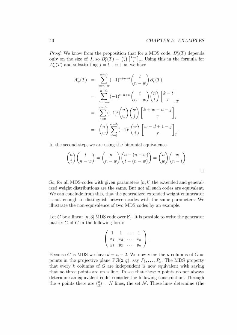
40 CHAPTER 5. EXAMPLES
Proof: We know from the proposition that for a MDS code, BrJ(T ) depends
only on the size of J , so Brt (T ) =
(nt
) [k−tr
]T
. Using this in the formula forAr
w(T ) and substituting j = t− n+ w, we have
Arw(T ) =
n−dr∑t=n−w
(−1)n+w+t
(t
n− w
)Br
t (T )
=n−dr∑
t=n−w
(−1)t−n+w
(t
n− w
)(n
t
)[k − tr
]T
=w−dr∑j=0
(−1)j
(n
w
)(w
j
)[k + w − n− j
r
]T
=
(n
w
) w−dr∑j=0
(−1)j
(w
j
)[w − d+ 1− j
r
]T
.
In the second step, we are using the binomial equivalence(n
t
)(t
n− w
)=
(n
n− w
)(n− (n− w)
t− (n− w)
)=
(n
w
)(w
n− t
).
�
So, for all MDS-codes with given parameters [n, k] the extended and general-ized weight distributions are the same. But not all such codes are equivalent.We can conclude from this, that the generalized extended weight enumeratoris not enough to distinguish between codes with the same parameters. Weillustrate the non-equivalence of two MDS codes by an example.
Let C be a linear [n, 3] MDS code over Fq. It is possible to write the generatormatrix G of C in the following form: 1 1 . . . 1
x1 x2 . . . xn
y1 y2 . . . yn
.
Because C is MDS we have d = n− 2. We now view the n columns of G aspoints in the projective plane PG(2, q), say P1, . . . , Pn. The MDS propertythat every k columns of G are independent is now equivalent with sayingthat no three points are on a line. To see that these n points do not alwaysdetermine an equivalent code, consider the following construction. Throughthe n points there are
(n2
)= N lines, the set N . These lines determine (the
5.2. TWO [6, 3] CODES 41
generator matrix of) a [N, 3] code C. The minimum distance of the code C isequal to the total number of lines minus the maximum number of lines fromN through an arbitrarily point P ∈ PG(2, q). If P /∈ {P1, . . . , Pn} then themaximum number of lines from N through P is at most 1
2n, since no three
points of N lie on a line. If P = Pi for some i ∈ [n] then P lies on exactlyn − 1 lines of N , namely the lines PiPj for j 6= i. Therefore the minimum
distance of C is d = N − n+ 1.We now have constructed a [N, 3, N − n + 1] code C from the original codeC. Notice that two codes C1 and C2 are equivalent if and only if C1 and C2
are equivalent. The (generalized extended) weight enumerators W rC(X, Y, T )
are completely determined, but this is not generally true for W rC
(X, Y, T ).
Take for example n = 4 and q = 4, so C is a [6, 3, 3] code. The six columns canbe viewed as six points in the projective plane. We know that every 5-tupleof points in the projective plane determines a unique conic. If we take five ofour six points and look at the conic they are on, there are three possibilitiesfor the last point: it can also be on the conic, it can be the nucleus of theconic (every tangent of the conic runs through the same point because q iseven), or it can be some other point. Every possibility can occur with d = 3for the final code, so not all [6, 3, 3] codes are equivalent. Therefore also notall [4, 3, 2] codes are equivalent.
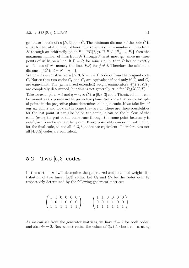
5.2 Two [6, 3] codes
In this section, we will determine the generalized and extended weight dis-tribution of two linear [6, 3] codes. Let C1 and C2 be the codes over F2
respectively determined by the following generator matrices:
1 1 0 0 0 01 0 1 0 0 01 1 1 1 1 1
,
1 1 0 0 0 00 0 1 1 0 01 1 1 1 1 1
.
As we can see from the generator matrices, we have d = 2 for both codes,and also d⊥ = 2. Now we determine the values of l(J) for both codes, using
42 CHAPTER 5. EXAMPLES
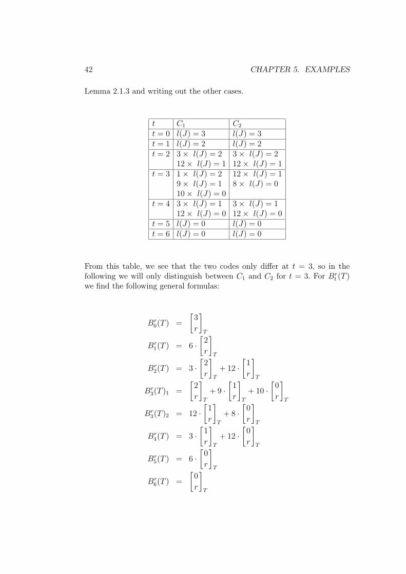
Lemma 2.1.3 and writing out the other cases.
t C1 C2
t = 0 l(J) = 3 l(J) = 3t = 1 l(J) = 2 l(J) = 2t = 2 3× l(J) = 2 3× l(J) = 2
12× l(J) = 1 12× l(J) = 1t = 3 1× l(J) = 2 12× l(J) = 1
9× l(J) = 1 8× l(J) = 010× l(J) = 0
t = 4 3× l(J) = 1 3× l(J) = 112× l(J) = 0 12× l(J) = 0
t = 5 l(J) = 0 l(J) = 0t = 6 l(J) = 0 l(J) = 0
From this table, we see that the two codes only differ at t = 3, so in thefollowing we will only distinguish between C1 and C2 for t = 3. For Br
t (T )we find the following general formulas:
Br0(T ) =
[3
r
]T
Br1(T ) = 6 ·
[2
r
]T
Br2(T ) = 3 ·
[2
r
]T
+ 12 ·[
1
r
]T
Br3(T )1 =
[2
r
]T
+ 9 ·[
1
r
]T
+ 10 ·[
0
r
]T
Br3(T )2 = 12 ·
[1
r
]T
+ 8 ·[
0
r
]T
Br4(T ) = 3 ·
[1
r
]T
+ 12 ·[
0
r
]T
Br5(T ) = 6 ·
[0
r
]T
Br6(T ) =
[0
r
]T
5.2. TWO [6, 3] CODES 43
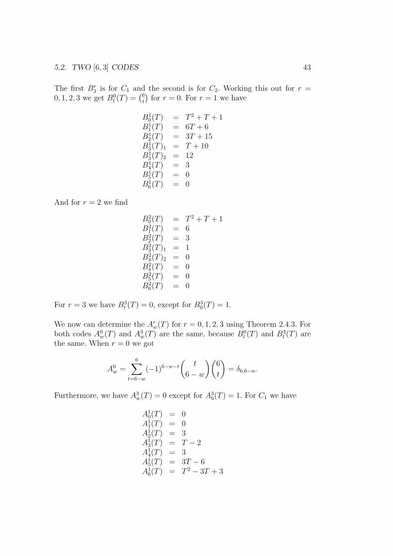
The first Br3 is for C1 and the second is for C2. Working this out for r =
0, 1, 2, 3 we get B0t (T ) =
(6t
)for r = 0. For r = 1 we have
B10(T ) = T 2 + T + 1
B11(T ) = 6T + 6
B12(T ) = 3T + 15
B13(T )1 = T + 10
B13(T )2 = 12
B14(T ) = 3
B15(T ) = 0
B16(T ) = 0
And for r = 2 we find
B20(T ) = T 2 + T + 1
B21(T ) = 6
B22(T ) = 3
B23(T )1 = 1
B23(T )2 = 0
B24(T ) = 0
B25(T ) = 0
B26(T ) = 0
For r = 3 we have B3t (T ) = 0, except for B3
0(T ) = 1.
We now can determine the Arw(T ) for r = 0, 1, 2, 3 using Theorem 2.4.3. For
both codes A0w(T ) and A3
w(T ) are the same, because B0t (T ) and B3
t (T ) arethe same. When r = 0 we got
A0w =
6∑t=6−w
(−1)6−w−t
(t
6− w
)(6
t
)= δ6,6−w.
Furthermore, we have A3w(T ) = 0 except for A3
6(T ) = 1. For C1 we have
A10(T ) = 0
A11(T ) = 0
A12(T ) = 3
A13(T ) = T − 2
A14(T ) = 3
A15(T ) = 3T − 6
A16(T ) = T 2 − 3T + 3
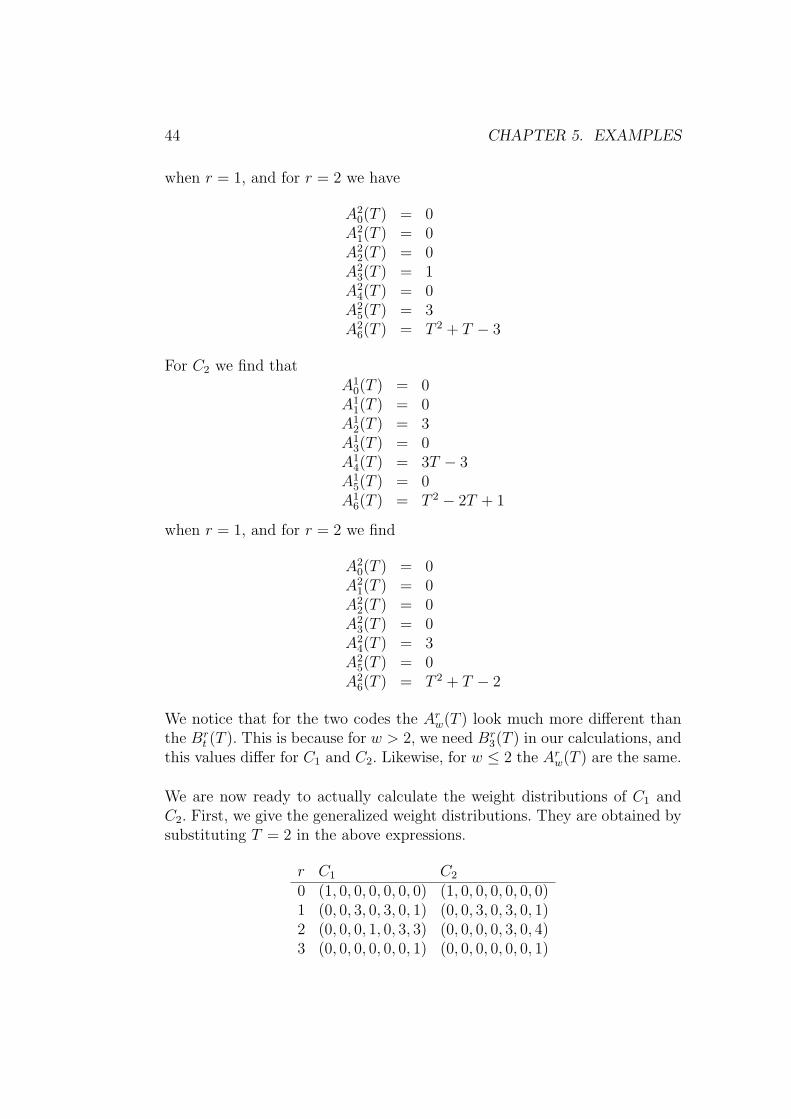
44 CHAPTER 5. EXAMPLES
when r = 1, and for r = 2 we have
A20(T ) = 0
A21(T ) = 0
A22(T ) = 0
A23(T ) = 1
A24(T ) = 0
A25(T ) = 3
A26(T ) = T 2 + T − 3
For C2 we find thatA1
0(T ) = 0A1
1(T ) = 0A1
2(T ) = 3A1
3(T ) = 0A1
4(T ) = 3T − 3A1
5(T ) = 0A1
6(T ) = T 2 − 2T + 1
when r = 1, and for r = 2 we find
A20(T ) = 0
A21(T ) = 0
A22(T ) = 0
A23(T ) = 0
A24(T ) = 3
A25(T ) = 0
A26(T ) = T 2 + T − 2
We notice that for the two codes the Arw(T ) look much more different than
the Brt (T ). This is because for w > 2, we need Br
3(T ) in our calculations, andthis values differ for C1 and C2. Likewise, for w ≤ 2 the Ar
w(T ) are the same.
We are now ready to actually calculate the weight distributions of C1 andC2. First, we give the generalized weight distributions. They are obtained bysubstituting T = 2 in the above expressions.
r C1 C2
0 (1, 0, 0, 0, 0, 0, 0) (1, 0, 0, 0, 0, 0, 0)1 (0, 0, 3, 0, 3, 0, 1) (0, 0, 3, 0, 3, 0, 1)2 (0, 0, 0, 1, 0, 3, 3) (0, 0, 0, 0, 3, 0, 4)3 (0, 0, 0, 0, 0, 0, 1) (0, 0, 0, 0, 0, 0, 1)
5.3. NOTES 45
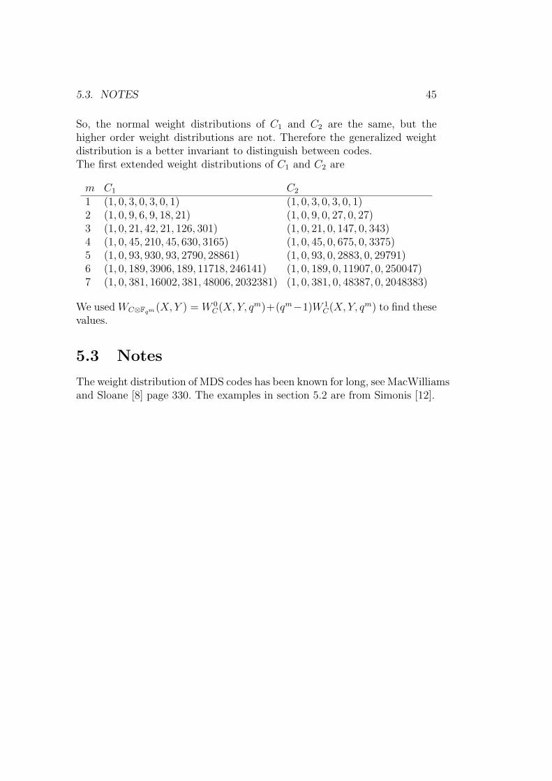
So, the normal weight distributions of C1 and C2 are the same, but thehigher order weight distributions are not. Therefore the generalized weightdistribution is a better invariant to distinguish between codes.The first extended weight distributions of C1 and C2 are
m C1 C2
1 (1, 0, 3, 0, 3, 0, 1) (1, 0, 3, 0, 3, 0, 1)2 (1, 0, 9, 6, 9, 18, 21) (1, 0, 9, 0, 27, 0, 27)3 (1, 0, 21, 42, 21, 126, 301) (1, 0, 21, 0, 147, 0, 343)4 (1, 0, 45, 210, 45, 630, 3165) (1, 0, 45, 0, 675, 0, 3375)5 (1, 0, 93, 930, 93, 2790, 28861) (1, 0, 93, 0, 2883, 0, 29791)6 (1, 0, 189, 3906, 189, 11718, 246141) (1, 0, 189, 0, 11907, 0, 250047)7 (1, 0, 381, 16002, 381, 48006, 2032381) (1, 0, 381, 0, 48387, 0, 2048383)
We used WC⊗Fqm (X, Y ) = W 0C(X, Y, qm)+(qm−1)W 1
C(X, Y, qm) to find thesevalues.
5.3 Notes
The weight distribution of MDS codes has been known for long, see MacWilliamsand Sloane [8] page 330. The examples in section 5.2 are from Simonis [12].
46 CHAPTER 5. EXAMPLES
Chapter 6
Implementation and complexity
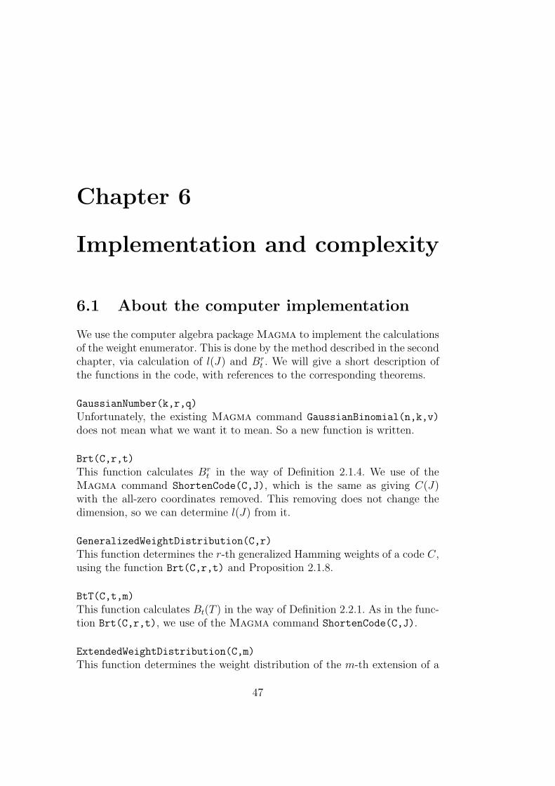
6.1 About the computer implementation
We use the computer algebra package Magma to implement the calculationsof the weight enumerator. This is done by the method described in the secondchapter, via calculation of l(J) and Br
t . We will give a short description ofthe functions in the code, with references to the corresponding theorems.
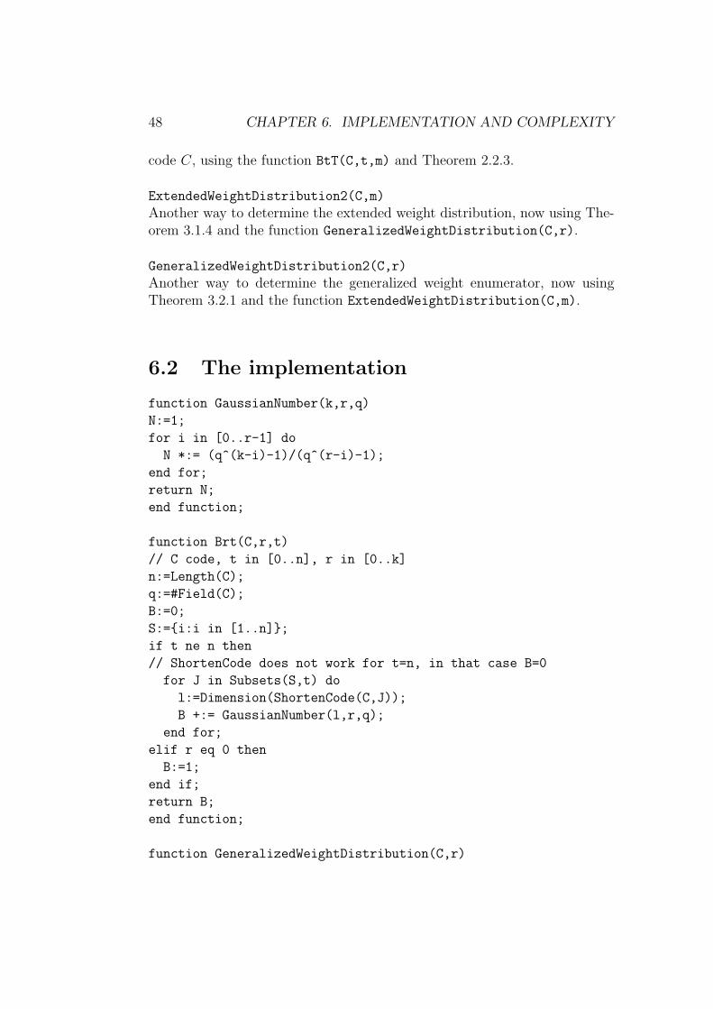
GaussianNumber(k,r,q)
Unfortunately, the existing Magma command GaussianBinomial(n,k,v)
does not mean what we want it to mean. So a new function is written.
Brt(C,r,t)
This function calculates Brt in the way of Definition 2.1.4. We use of the
Magma command ShortenCode(C,J), which is the same as giving C(J)with the all-zero coordinates removed. This removing does not change thedimension, so we can determine l(J) from it.
GeneralizedWeightDistribution(C,r)
This function determines the r-th generalized Hamming weights of a code C,using the function Brt(C,r,t) and Proposition 2.1.8.
BtT(C,t,m)
This function calculates Bt(T ) in the way of Definition 2.2.1. As in the func-tion Brt(C,r,t), we use of the Magma command ShortenCode(C,J).
ExtendedWeightDistribution(C,m)
This function determines the weight distribution of the m-th extension of a
47
48 CHAPTER 6. IMPLEMENTATION AND COMPLEXITY
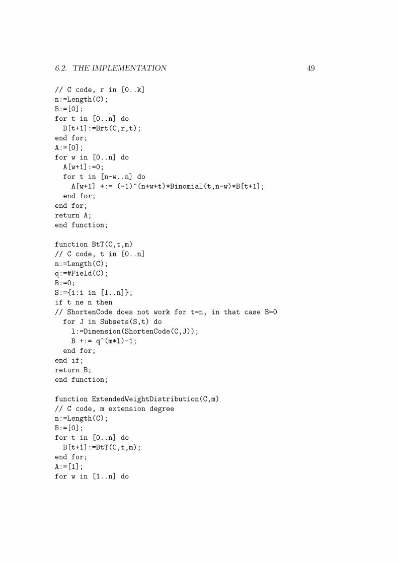
code C, using the function BtT(C,t,m) and Theorem 2.2.3.
ExtendedWeightDistribution2(C,m)
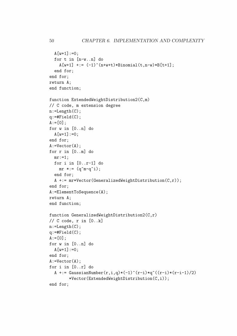
Another way to determine the extended weight distribution, now using The-orem 3.1.4 and the function GeneralizedWeightDistribution(C,r).
GeneralizedWeightDistribution2(C,r)
Another way to determine the generalized weight enumerator, now usingTheorem 3.2.1 and the function ExtendedWeightDistribution(C,m).
6.2 The implementation
function GaussianNumber(k,r,q)
N:=1;
for i in [0..r-1] do
N *:= (q^(k-i)-1)/(q^(r-i)-1);
end for;
return N;
end function;
function Brt(C,r,t)
// C code, t in [0..n], r in [0..k]
n:=Length(C);
q:=#Field(C);
B:=0;
S:={i:i in [1..n]};
if t ne n then
// ShortenCode does not work for t=n, in that case B=0
for J in Subsets(S,t) do
l:=Dimension(ShortenCode(C,J));
B +:= GaussianNumber(l,r,q);
end for;
elif r eq 0 then
B:=1;
end if;
return B;
end function;
function GeneralizedWeightDistribution(C,r)
6.2. THE IMPLEMENTATION 49
// C code, r in [0..k]
n:=Length(C);
B:=[0];
for t in [0..n] do
B[t+1]:=Brt(C,r,t);
end for;
A:=[0];
for w in [0..n] do
A[w+1]:=0;
for t in [n-w..n] do
A[w+1] +:= (-1)^(n+w+t)*Binomial(t,n-w)*B[t+1];
end for;
end for;
return A;
end function;
function BtT(C,t,m)
// C code, t in [0..n]
n:=Length(C);
q:=#Field(C);
B:=0;
S:={i:i in [1..n]};
if t ne n then
// ShortenCode does not work for t=n, in that case B=0
for J in Subsets(S,t) do
l:=Dimension(ShortenCode(C,J));
B +:= q^(m*l)-1;
end for;
end if;
return B;
end function;
function ExtendedWeightDistribution(C,m)
// C code, m extension degree
n:=Length(C);
B:=[0];
for t in [0..n] do
B[t+1]:=BtT(C,t,m);
end for;
A:=[1];
for w in [1..n] do
50 CHAPTER 6. IMPLEMENTATION AND COMPLEXITY
A[w+1]:=0;
for t in [n-w..n] do
A[w+1] +:= (-1)^(n+w+t)*Binomial(t,n-w)*B[t+1];
end for;
end for;
return A;
end function;
function ExtendedWeightDistribution2(C,m)
// C code, m extension degree
n:=Length(C);
q:=#Field(C);
A:=[0];
for w in [0..n] do
A[w+1]:=0;
end for;
A:=Vector(A);
for r in [0..m] do
mr:=1;
for i in [0..r-1] do
mr *:= (q^m-q^i);
end for;
A +:= mr*Vector(GeneralizedWeightDistribution(C,r));
end for;
A:=ElementToSequence(A);
return A;
end function;
function GeneralizedWeightDistribution2(C,r)
// C code, r in [0..k]
n:=Length(C);
q:=#Field(C);
A:=[0];
for w in [0..n] do
A[w+1]:=0;
end for;
A:=Vector(A);
for i in [0..r] do
A +:= GaussianNumber(r,i,q)*(-1)^(r-i)*q^((r-i)*(r-i-1)/2)
*Vector(ExtendedWeightDistribution(C,i));
end for;
6.3. EXAMPLE: THE TERNARY GOLAY CODE 51
rr:=1;
for i in [0..r-1] do
rr *:= (q^r-q^i);
end for;
A:=ElementToSequence(A);
for w in [0..n] do
A[w+1] /:= rr;
end for;
return A;
end function;
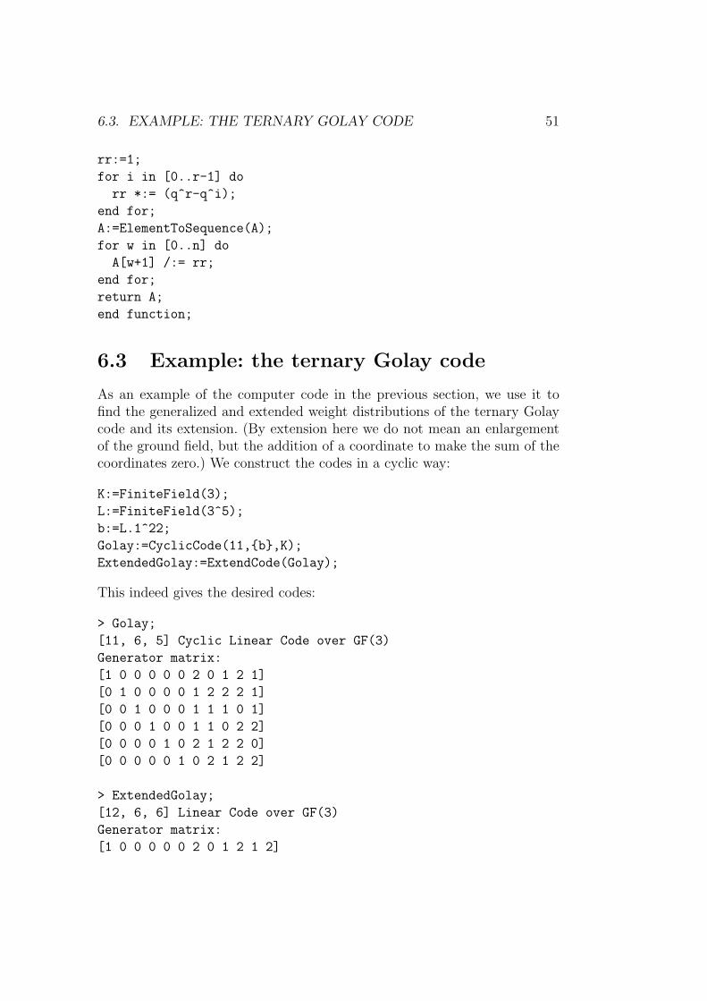
6.3 Example: the ternary Golay code
As an example of the computer code in the previous section, we use it tofind the generalized and extended weight distributions of the ternary Golaycode and its extension. (By extension here we do not mean an enlargementof the ground field, but the addition of a coordinate to make the sum of thecoordinates zero.) We construct the codes in a cyclic way:
K:=FiniteField(3);
L:=FiniteField(3^5);
b:=L.1^22;
Golay:=CyclicCode(11,{b},K);
ExtendedGolay:=ExtendCode(Golay);
This indeed gives the desired codes:
> Golay;
[11, 6, 5] Cyclic Linear Code over GF(3)
Generator matrix:
[1 0 0 0 0 0 2 0 1 2 1]
[0 1 0 0 0 0 1 2 2 2 1]
[0 0 1 0 0 0 1 1 1 0 1]
[0 0 0 1 0 0 1 1 0 2 2]
[0 0 0 0 1 0 2 1 2 2 0]
[0 0 0 0 0 1 0 2 1 2 2]
> ExtendedGolay;
[12, 6, 6] Linear Code over GF(3)
Generator matrix:
[1 0 0 0 0 0 2 0 1 2 1 2]
52 CHAPTER 6. IMPLEMENTATION AND COMPLEXITY
[0 1 0 0 0 0 1 2 2 2 1 0]
[0 0 1 0 0 0 1 1 1 0 1 1]
[0 0 0 1 0 0 1 1 0 2 2 2]
[0 0 0 0 1 0 2 1 2 2 0 1]
[0 0 0 0 0 1 0 2 1 2 2 1]
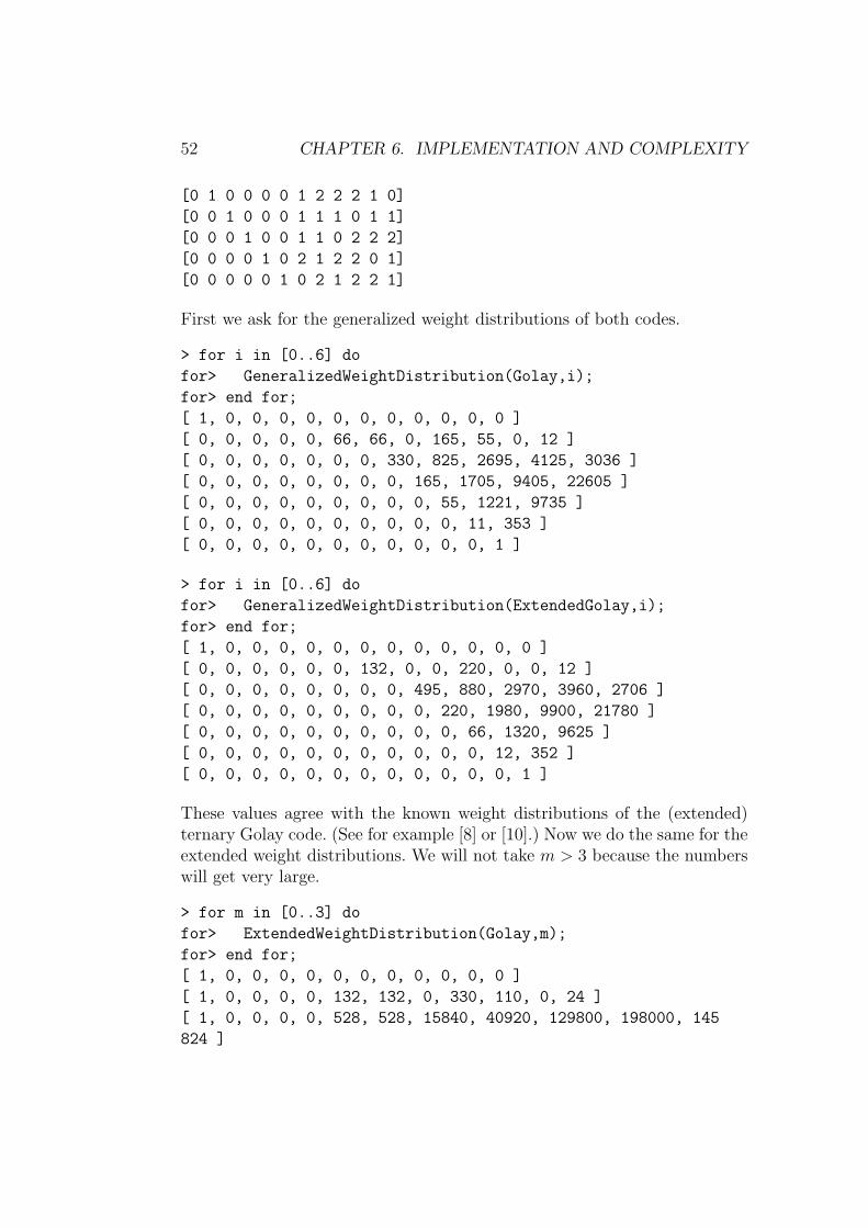
First we ask for the generalized weight distributions of both codes.
> for i in [0..6] do
for> GeneralizedWeightDistribution(Golay,i);
for> end for;
[ 1, 0, 0, 0, 0, 0, 0, 0, 0, 0, 0, 0 ]
[ 0, 0, 0, 0, 0, 66, 66, 0, 165, 55, 0, 12 ]
[ 0, 0, 0, 0, 0, 0, 0, 330, 825, 2695, 4125, 3036 ]
[ 0, 0, 0, 0, 0, 0, 0, 0, 165, 1705, 9405, 22605 ]
[ 0, 0, 0, 0, 0, 0, 0, 0, 0, 55, 1221, 9735 ]
[ 0, 0, 0, 0, 0, 0, 0, 0, 0, 0, 11, 353 ]
[ 0, 0, 0, 0, 0, 0, 0, 0, 0, 0, 0, 1 ]
> for i in [0..6] do
for> GeneralizedWeightDistribution(ExtendedGolay,i);
for> end for;
[ 1, 0, 0, 0, 0, 0, 0, 0, 0, 0, 0, 0, 0 ]
[ 0, 0, 0, 0, 0, 0, 132, 0, 0, 220, 0, 0, 12 ]
[ 0, 0, 0, 0, 0, 0, 0, 0, 495, 880, 2970, 3960, 2706 ]
[ 0, 0, 0, 0, 0, 0, 0, 0, 0, 220, 1980, 9900, 21780 ]
[ 0, 0, 0, 0, 0, 0, 0, 0, 0, 0, 66, 1320, 9625 ]
[ 0, 0, 0, 0, 0, 0, 0, 0, 0, 0, 0, 12, 352 ]
[ 0, 0, 0, 0, 0, 0, 0, 0, 0, 0, 0, 0, 1 ]
These values agree with the known weight distributions of the (extended)ternary Golay code. (See for example [8] or [10].) Now we do the same for theextended weight distributions. We will not take m > 3 because the numberswill get very large.
> for m in [0..3] do
for> ExtendedWeightDistribution(Golay,m);
for> end for;
[ 1, 0, 0, 0, 0, 0, 0, 0, 0, 0, 0, 0 ]
[ 1, 0, 0, 0, 0, 132, 132, 0, 330, 110, 0, 24 ]
[ 1, 0, 0, 0, 0, 528, 528, 15840, 40920, 129800, 198000, 145
824 ]

6.4. COMPLEXITY CALCULATIONS 53
[ 1, 0, 0, 0, 0, 1716, 1716, 205920, 2372370, 20833670, 1082
10
960, 255794136 ]
> for m in [0..3] do
for> ExtendedWeightDistribution(ExtendedGolay,m);
for> end for;
[ 1, 0, 0, 0, 0, 0, 0, 0, 0, 0, 0, 0, 0 ]
[ 1, 0, 0, 0, 0, 0, 264, 0, 0, 440, 0, 0, 24 ]
[ 1, 0, 0, 0, 0, 0, 1056, 0, 23760, 44000, 142560, 190080, 1
29984 ]
[ 1, 0, 0, 0, 0, 0, 3432, 0, 308880, 3025880, 24092640, 1136
67840,
246321816 ]
It is also possible to do the above calculations with the alternative functionsGeneralizedWeighDistribution2(C,r) which uses the extended weight enu-merator, and ExtendedWeightDistribution2(C,m), which use the general-ized weight enumerator. These functions give the same values, but the secondfunctions are much slower.
6.4 Complexity calculations
We discussed multiple ways to determine the weight enumerator of a linearcode. In this chapter, we look at the complexity of these calculations.
Definition 6.4.1 The complexity Comp(n,R) of the calculation of the weightenumerator of a linear [n, k] code over Fq with information rate R = k
nis
given as a function of n and R. The exponent of this function is defined as
E(R) = limn→∞
logq Comp(n,R)
n.
Remark that the complexity also depends on the used algorithm. Which al-gorithm is used, should be clear from the context.
The most straightforward way to calculate the weight enumerator is the bruteforce-method: we simply go through all words and determining their weight.There are qk words of length n, so the complexity of this brute force-methodis nqk and therefore E(R) = R. Because of the MacWilliams relations, we
54 CHAPTER 6. IMPLEMENTATION AND COMPLEXITY
may assume R ≤ 12.
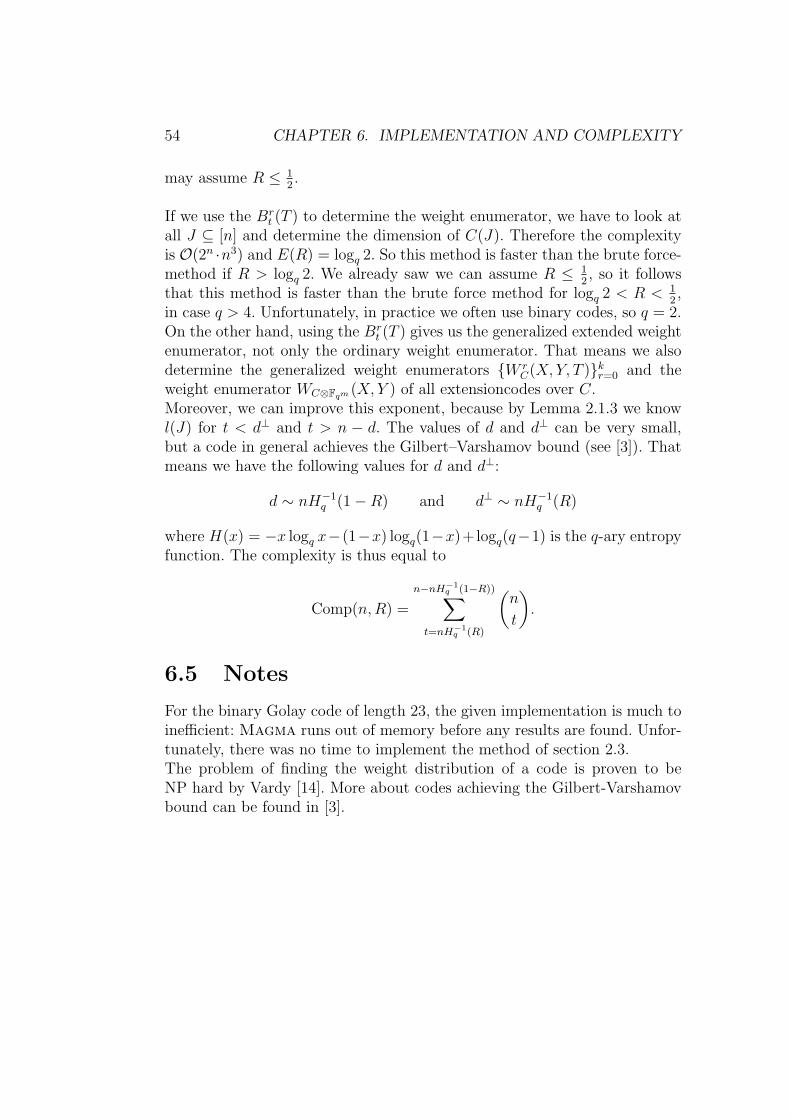
If we use the Brt (T ) to determine the weight enumerator, we have to look at
all J ⊆ [n] and determine the dimension of C(J). Therefore the complexityis O(2n ·n3) and E(R) = logq 2. So this method is faster than the brute force-method if R > logq 2. We already saw we can assume R ≤ 1
2, so it follows
that this method is faster than the brute force method for logq 2 < R < 12,
in case q > 4. Unfortunately, in practice we often use binary codes, so q = 2.On the other hand, using the Br
t (T ) gives us the generalized extended weightenumerator, not only the ordinary weight enumerator. That means we alsodetermine the generalized weight enumerators {W r
C(X, Y, T )}kr=0 and theweight enumerator WC⊗Fqm (X, Y ) of all extensioncodes over C.Moreover, we can improve this exponent, because by Lemma 2.1.3 we knowl(J) for t < d⊥ and t > n − d. The values of d and d⊥ can be very small,but a code in general achieves the Gilbert–Varshamov bound (see [3]). Thatmeans we have the following values for d and d⊥:
d ∼ nH−1q (1−R) and d⊥ ∼ nH−1
q (R)
where H(x) = −x logq x−(1−x) logq(1−x)+logq(q−1) is the q-ary entropyfunction. The complexity is thus equal to
Comp(n,R) =
n−nH−1q (1−R))∑
t=nH−1q (R)
(n
t
).
6.5 Notes
For the binary Golay code of length 23, the given implementation is much toinefficient: Magma runs out of memory before any results are found. Unfor-tunately, there was no time to implement the method of section 2.3.The problem of finding the weight distribution of a code is proven to beNP hard by Vardy [14]. More about codes achieving the Gilbert-Varshamovbound can be found in [3].
Chapter 7
Conclusions
In the second chapter, we described ways to determine the generalized weightenumerator, the extended weight enumerator and the generalized extendedweight enumerator. These methods are very similar and based on the determi-nation of l(J) for all J ⊆ [n], where l(J) = dim{c ∈ C : cj = 0 for all j ∈ J}.Besides this method, we discovered a way to determine the extended weightenumerator by matrix decomposition.It tuns out that the generalized weight enumerators, the extended weightenumerator and the Tutte polynomial all contain the same amount of infor-mation about a code (or matroid). This is a better invariant then the originalweight enumerator. All the in between links have been made explicit and anoverview can be found in section 3.4. Further extension or generalization doesnot give more information about the code.For the three equivalent polynomials we proved MacWilliams-like relationsbetween the polynomial and the polynomial of the dual object – code or ma-troid. With use of the language described in the second chapter, we simplifiedknown results and proved their equivalence. Using Br
t (T ) in the definition ofthe weight enumerators turns out to be quite useful. Also, we gave examplesof the theory.
55

56 CHAPTER 7. CONCLUSIONS
Bibliography
[1] R.E. Blahut. Algebraic Codes for Data Transmission. Camebridge Uni-versity Press, Camebridge, 2003.
[2] T.H. Brylawsky and J.G. Oxley. The tutte polynomial and its applica-tions. In N. White, editor, Matroid Applications. Cambridge UniversityPress, Cambridge, 1992.
[3] J.T. Coffey and R.M. Goodman. Any code of which we cannot think isgood. IEEE Transactions on Information Theory, 36:1453–1461, 1990.
[4] C. Greene. Weight enumeration and the geometry of linear codes. Stud-ies in Applied Mathematics, 55:119–128, 1976.
[5] G.L. Katsman and M.A. Tsfasman. Spectra of algebraic-geometriccodes. Problemy Peredachi Informatsii, 23:19–34, 1987.
[6] T. Kløve. The weight distribution of linear codes over GF(ql) havinggenerator matrix over GF(q)∗. Discrete Mathematics, 23:159–168, 1978.
[7] T. Kløve. Support weight distribution of linear codes. Discrete Matem-atics, 106/107:311–316, 1992.
[8] F.J. MacWilliams and N.J.A. Sloane. The Theory of Error-CorrectingCodes. North-Holland Mathematical Library, Amsterdam, 1977.
[9] J.G. Oxley. Matroid theory. Oxford University Press, Oxford, 1992.
[10] R. Pellikaan, X.-W. Wu, and S. Bulygin. Codes and cryptography onalgebraic curves. preliminary version, to be published by CambridgeUniversity Press, 2008.
[11] J. Riordan. Combinatorial Identities. Robert E. Krieger PublishingCompany, New York, 1979.
[12] J. Simonis. The effective length of subcodes. AAECC, 5:371–377, 1993.
57
58 BIBLIOGRAPHY
[13] M.A. Tsfasman and S.G. Vladut. Algebraic-geometric codes. KluwerAcademic Publishers, Dordrecht, 1991.
[14] A. Vardy. The intractibility of computing the minimum distance of acode. IEEE Transactions on Information Theory, 43:1757–1766, 1997.
[15] V.K. Wei. Generalized Hamming weights for linear codes. IEEE Trans-actions on Information Theory, 37:1412–1418, 1991.