cleaning correlation matrices - cfm · cleaning correlation matrices the determination of...

Cleaning correlation matricesA new cleaning recipe that outperforms all existing estimators in terms of the out-of-sample risk of synthetic portfolios

Risk.net April 2016

Risk management • deRivatives • Regulation

RePRinted FRom

Cutting edgeRefining Markowitz

�

�

�

�

�

�

�

�

Cutting edge investments: Portfolio management

section, also the most efficient.1 In the following, � denotes a cleanedestimator of the true correlation matrix C and ˛ 2 Œ0; 1� is a parameterthat must be determined through optimisation or analytical arguments.� 1. Basic linear shrinkage: a linear combination of the sampleestimate and the identity matrix:

�bas: WD ˛E C .1 � ˛/IN (3)

This is probably the oldest method proposed in the literature (Haff1980). In a financial context, this method can be seen as a heuristicway to control the diversification of the optimal Markowitz portfolio(Bouchaud & Potters 2003).� 2. Advanced linear shrinkage: a linear combination of the sampleestimate and a correlation matrix containing the market mode:

� adv: WD ˛E C .1 � ˛/Œ.1 � �/IN C �ee�� (4)

where e D .1; 1; : : : ; 1/ is the unit vector and � an average correlationthat can be optimally and self-consistently estimated (see Ledoit &Wolf 2003). It turns out, however, that (4) provides similar performanceto (3) (Ledoit & Wolf 2014).� 3. Eigenvalues clipping (Bouchaud & Potters 2011): keep the dN˛etop eigenvalues and shrink the others to a constant � that preserves thetrace, Tr.� clip:/ D Tr.E/ D N :

� clip: WDNX

kD1

�clip:

kuku�

k ; �clip:

kWD

(�k if k 6 dN˛e� otherwise

(5)

A simple (but ad hoc) procedure to choose ˛ is to assume that allempirical eigenvalues beyond the Marcenko and Pastur upper edge(see Box 1) can be deemed to contain some signal and are thereforekept without change. However, this cleaning overlooks the fact thatthe large empirical eigenvalues are overestimated (see below).� 4. Eigenvalues substitution: sample eigenvalues �k are replaced byan estimation �k of the true ones, obtained by inverting the generalMarcenko and Pastur equation relating the spectrum of C to that of E :

� sub: WDNX

kD1

�sub:k uku�

k (6)

The inversion of the Marcenko-Pastur equation is numerically unstableand requires either a parametric description of the spectrum of C (eg, apower law, as proposed in Bouchaud & Potters (2011)) or some priorknowledge of the location of the ‘true’ eigenvalues as in El Karoui(2008). This method is also sub-optimal on theoretical grounds as itfails to take into account the noise in the eigenvector determination.� 5. Rotationally invariant, optimal shrinkage: this method was firstproposed by Ledoit & Péché (2011), who realised that one can actuallycompute the ‘overlap’between true and sample eigenvectors, preciselythe ingredient missing from method 4. The method was extended todiscrete eigenvalues (including outliers) in Bun & Knowles (2016)which also provided a practical implementation. The method was fur-ther studied in Bun, Bouchaud & Potters (2016), where, in particu-lar, an ad hoc method was proposed to correct for a systematic bias

1 There are of course many other estimators in the literature, but we onlykeep estimators that seem relevant for this problem, at least to our eyes.

for small eigenvalues. For large N , the optimal rotational invariantestimator (RIE) of C reads:

�RIE WDNX

kD1

�RIEk uku�

k

with (Bun & Knowles 2016):

�RIEk WD �k

j1 � q C qzks.zk/j2 (7)

where s.z/ WD N �1 tr.zIN � E/�1 and zk D �k � i� (see belowfor the chosen value of �). The rotational invariant hypothesis on anestimator � assumes that one does not have any prior knowledge ofthe structure of the true eigenvectors, and therefore that the best onecan do is to keep the eigenvectors ui of E untouched.2

We will not discuss methods 2 and 4 any further, because they turnout to be less efficient than the simpler schemes 1 and 3 on real data.Also, we do not consider the algorithm of Ledoit & Wolf (2014) formethod 5 because it requires heavy numerical operations with O.N /

parameters to fit. Moreover, the proposed quantile representation rulesout a priori outliers (see Bun & Knowles (2016) for an extended discus-sion on this topic). Equation (7), on the other hand, is very appealingfrom a theoretical point of view. The optimality of (7) stands in thefollowing sense. Suppose that we knew C exactly, but constrain our-selves to estimate it in the eigenbasis fukg of E . The optimal estimatorof the eigenvalues of C would then read:

�ora:k WD huk ; Cuki (8)

where h�; �i denotes the inner product. Note that the superscript ‘ora.’stands for oracle, which is the optimal estimator that one would obtainif one knew the true correlation matrix C (which is of course not thecase, since we are actually attempting to estimate C !). But, as wasshown in Bun & Knowles (2016), (7) satisfies, roughly speaking:

j�RIEk � huk ; Cukij D O.T �1=2/ 8k (9)

for q D O.1/. This means that the estimator �RIEk

converges, for largeenough T , to the optimal ‘oracle’ estimator (8).

For practical applications, however, (7) contains a parameter � thatmust be chosen to be small, but at the same time such that N� � 1.A good trade-off is to set � D N �1=2 (see Bun & Knowles 2016).Unfortunately, in cases where N is not extremely large (say N D400), this corresponds to � D 0:05, which is not very small, andthis induces a systematic downward bias in the estimator of smalleigenvalues (see Bun, Bouchaud & Potters (2016) for an extendeddiscussion of this point). This bias can be explicitly calculated in simplecases and suggests the following heuristic correction for any k:3

O�k WD �RIEk � max.1; �k/ (10)

2 This assumption is certainly not true of the market mode itself, and possi-bly of all the spikes corresponding to sectors. However, this is the simplestassumption that should be reasonable for the bulk of C and that can beimproved upon (see, for example, Monasson & Villamaina 2015).3 This correction is fit for the case of stock markets on which we focusin this note. In the case of futures markets, the presence of very stronglycorrelated contracts (ie, two different maturities for the same underlying)leads to very small true eigenvalues of the correlation matrix, and requiresa more sophisticated regularisation (see Bun, Bouchaud & Potters 2016).

risk.net 55

�

�

�

�

�

�

�

�


Cleaning correlation matricesThe determination of correlation matrices is typically affected by in-sample noise. Joël Bun, Jean-Philippe Bouchaud andMarc Potters propose a simple, yet optimal, estimator of the true underlying correlation matrix and show that this newcleaning recipe outperforms all existing estimators in terms of the out-of-sample risk of synthetic portfolios

The concept of correlations between different assets is a cor-nerstone of Markowitz’s optimal portfolio theory, especiallyfor risk management purposes (Markowitz 1968). In a nut-shell, correlations measure the tendency of different assets

to vary together, and it is well known that large losses at a portfoliolevel are indeed mostly due to correlated moves of its constituents (see,for example, Bouchaud & Potters 2003). Efficient and robust diversi-fication is needed to alleviate such events. Markowitz’s theory is thesimplest and best known method for constructing a portfolio with agiven level of risk, using the correlations between assets as inputs.However, the Markowitz solution results in over-allocation on lowvariance modes (ie, eigenvectors) of the correlation matrix. It is there-fore of crucial importance to use a correlation matrix that faithfullyrepresents future, and not past, risks – otherwise the over-allocation onspurious low risk combinations of assets might prove disastrous (see,for example, Bouchaud & Potters (2011) for a detailed discussion ofthis point).

The question of building reliable estimators of covariance or ofcorrelation matrices has a long history in finance, and more generallyin multivariate statistical analysis. The problem comes from the high-dimensionality of these matrices, as in many applications. When thesize of the time series T is very large, each of the coefficients of thecovariance/correlation matrix can be estimated with negligible error (ifis assumed not to vary with time). But if N is also large and of the orderof T , as is often the case in finance, the large number of noisy variablescreates important systematic errors in the computation of the inverseof the matrix, which is a direct input of Markowitz’s optimisationformula. These systematic errors lead to sub-optimal portfolios withgrossly underestimated out-of-sample risk (Bouchaud & Potters 2011).

The aim of this note is to provide the reader with a short review ofthe different cleaning ‘recipes’that have been proposed in the literatureto cope with the problem of in-sample noise in the determination ofcorrelation matrices. While some of these recipes are simple and wellknown, recent progress has been made that allows one to derive anoptimal and fully observable estimator of the ‘true’ underlying corre-lation matrix, valid in the limit of large matrices. We want to popularisethese new results and test the corresponding estimators on real finan-cial data, with very satisfactory benefits: both the realised risk andrisk-adjusted returns of synthetic portfolios are improved for a wideclass of investment strategies.

Setting the stageWe consider a universe made of N different financial assets that weobserve at (say) the daily frequency, defining a vector of returnsrt D .r1t ; r2t ; : : : ; rNt / for each day t D 1; : : : ; T . Because theaim of the present study is to focus specifically on correlations and not

on volatilities, we standardise these returns as follows: (i) we removethe sample mean of each asset; (ii) we normalise each return by anestimate O�it of its daily volatility, Qrit WD rit = O�it . There are many pos-sible choices for O�it , based on, for example, Garch or Figarch modelshistorical returns, or simply implied volatilities from option markets,and the reader can choose his/her favourite estimator which can easilybe combined with the correlation matrix cleaning schemes discussedbelow. For simplicity, we have chosen here the cross-sectional dailyvolatility, that is:

O�it DsX

j

r2jt

to remove a substantial amount of non-stationarity in the volatilities.The final standardised return matrix X D .Xit / 2 RN �T is thengiven by Xit WD Qrit =�i , where �i is the sample estimator of thevolatility of Qri , which is now, to a first approximation, stationary.

The most common (and simplest) estimator of the ‘true’ underlyingcorrelation matrix (that we henceforth denote by C ) is to use the sampleestimator:

E WD 1

TXX� (1)

We will use the following notation throughout:

E DNX

kD1

�kuku�k (2)

for the eigenvalues �1 > �2 > � � � > �N > 0 and the associatedeigenvectors u1; u2; : : : ; uN of E . When q D N=T ! 0, ie, whenthe data set is very long, one expects that E ! C , whereas impor-tant distortions survive when q D O.1/, even if T ! 1. In fact,since the work of Marcenko & Pastur (1967) decades ago, one canshow that the spectrum of E is a broadened version of that of C ,with an explicit q-dependent formula relating the two. In particular,small �i s are too small and large �i s are too large compared to thetrue eigenvalues C . Thus, recalling that Markowitz’s optimal strat-egy overweight low variance modes (see, for example, Bouchaud &Potters 2011), we understand why using the sample estimator E canlead to disastrous results, and why some cleaning procedure shouldbe applied to E before any application to portfolio construction. Notethat the Marcenko and Pastur results do not require multivariate nor-mality of the returns, which can have fat-tailed distributions. In fact,the above normalisation by the cross-sectional volatility can be seenas a proxy for a robust estimator of the covariance matrix (see, forexample, Couillet, Kammoun & Pascal 2016).

Five cleaning recipesWe list here five estimators that have been proposed in the literature,the last one being the most recent and, as we shall see in the next

54 risk.net December 2015


Reprinted from Risk April 2016

�

�

�

�

�

�

�

�


section, also the most efficient.1 In the following, � denotes a cleanedestimator of the true correlation matrix C and ˛ 2 Œ0; 1� is a parameterthat must be determined through optimisation or analytical arguments.� 1. Basic linear shrinkage: a linear combination of the sampleestimate and the identity matrix:

�bas: WD ˛E C .1 � ˛/IN (3)

This is probably the oldest method proposed in the literature (Haff1980). In a financial context, this method can be seen as a heuristicway to control the diversification of the optimal Markowitz portfolio(Bouchaud & Potters 2003).� 2. Advanced linear shrinkage: a linear combination of the sampleestimate and a correlation matrix containing the market mode:

� adv: WD ˛E C .1 � ˛/Œ.1 � �/IN C �ee�� (4)

where e D .1; 1; : : : ; 1/ is the unit vector and � an average correlationthat can be optimally and self-consistently estimated (see Ledoit &Wolf 2003). It turns out, however, that (4) provides similar performanceto (3) (Ledoit & Wolf 2014).� 3. Eigenvalues clipping (Bouchaud & Potters 2011): keep the dN˛etop eigenvalues and shrink the others to a constant � that preserves thetrace, Tr.� clip:/ D Tr.E/ D N :

� clip: WDNX

kD1

�clip:

kuku�

k ; �clip:

kWD

(�k if k 6 dN˛e� otherwise

(5)

A simple (but ad hoc) procedure to choose ˛ is to assume that allempirical eigenvalues beyond the Marcenko and Pastur upper edge(see Box 1) can be deemed to contain some signal and are thereforekept without change. However, this cleaning overlooks the fact thatthe large empirical eigenvalues are overestimated (see below).� 4. Eigenvalues substitution: sample eigenvalues �k are replaced byan estimation �k of the true ones, obtained by inverting the generalMarcenko and Pastur equation relating the spectrum of C to that of E :

� sub: WDNX

kD1

�sub:k uku�

k (6)

The inversion of the Marcenko-Pastur equation is numerically unstableand requires either a parametric description of the spectrum of C (eg, apower law, as proposed in Bouchaud & Potters (2011)) or some priorknowledge of the location of the ‘true’ eigenvalues as in El Karoui(2008). This method is also sub-optimal on theoretical grounds as itfails to take into account the noise in the eigenvector determination.� 5. Rotationally invariant, optimal shrinkage: this method was firstproposed by Ledoit & Péché (2011), who realised that one can actuallycompute the ‘overlap’between true and sample eigenvectors, preciselythe ingredient missing from method 4. The method was extended todiscrete eigenvalues (including outliers) in Bun & Knowles (2016)which also provided a practical implementation. The method was fur-ther studied in Bun, Bouchaud & Potters (2016), where, in particu-lar, an ad hoc method was proposed to correct for a systematic bias

1 There are of course many other estimators in the literature, but we onlykeep estimators that seem relevant for this problem, at least to our eyes.

for small eigenvalues. For large N , the optimal rotational invariantestimator (RIE) of C reads:

�RIE WDNX

kD1

�RIEk uku�

k

with (Bun & Knowles 2016):

�RIEk WD �k

j1 � q C qzks.zk/j2 (7)

where s.z/ WD N �1 tr.zIN � E/�1 and zk D �k � i� (see belowfor the chosen value of �). The rotational invariant hypothesis on anestimator � assumes that one does not have any prior knowledge ofthe structure of the true eigenvectors, and therefore that the best onecan do is to keep the eigenvectors ui of E untouched.2

We will not discuss methods 2 and 4 any further, because they turnout to be less efficient than the simpler schemes 1 and 3 on real data.Also, we do not consider the algorithm of Ledoit & Wolf (2014) formethod 5 because it requires heavy numerical operations with O.N /

parameters to fit. Moreover, the proposed quantile representation rulesout a priori outliers (see Bun & Knowles (2016) for an extended discus-sion on this topic). Equation (7), on the other hand, is very appealingfrom a theoretical point of view. The optimality of (7) stands in thefollowing sense. Suppose that we knew C exactly, but constrain our-selves to estimate it in the eigenbasis fukg of E . The optimal estimatorof the eigenvalues of C would then read:

�ora:k WD huk ; Cuki (8)

where h�; �i denotes the inner product. Note that the superscript ‘ora.’stands for oracle, which is the optimal estimator that one would obtainif one knew the true correlation matrix C (which is of course not thecase, since we are actually attempting to estimate C !). But, as wasshown in Bun & Knowles (2016), (7) satisfies, roughly speaking:

j�RIEk � huk ; Cukij D O.T �1=2/ 8k (9)

for q D O.1/. This means that the estimator �RIEk

converges, for largeenough T , to the optimal ‘oracle’ estimator (8).

For practical applications, however, (7) contains a parameter � thatmust be chosen to be small, but at the same time such that N� � 1.A good trade-off is to set � D N �1=2 (see Bun & Knowles 2016).Unfortunately, in cases where N is not extremely large (say N D400), this corresponds to � D 0:05, which is not very small, andthis induces a systematic downward bias in the estimator of smalleigenvalues (see Bun, Bouchaud & Potters (2016) for an extendeddiscussion of this point). This bias can be explicitly calculated in simplecases and suggests the following heuristic correction for any k:3

O�k WD �RIEk � max.1; �k/ (10)

2 This assumption is certainly not true of the market mode itself, and possi-bly of all the spikes corresponding to sectors. However, this is the simplestassumption that should be reasonable for the bulk of C and that can beimproved upon (see, for example, Monasson & Villamaina 2015).3 This correction is fit for the case of stock markets on which we focusin this note. In the case of futures markets, the presence of very stronglycorrelated contracts (ie, two different maturities for the same underlying)leads to very small true eigenvalues of the correlation matrix, and requiresa more sophisticated regularisation (see Bun, Bouchaud & Potters 2016).

risk.net 55


Risk April 2016

�

�

�

�

�

�

�

�


2 Comparison of the debiased RIE (10) (the blue line) with clip-ping at the edge of the Marcenko-Pastur (the red dashed line)and the linear shrinkage with ˛ D 0.5 (green dotted line)

0 1 2 3 4 50

1

2

3

4

5

ClippingLinearRIE

λ

ξ

We use the same data set as in figure 1

only sensitive to the quality of the estimator of the correlation matrixitself.

In order to ascertain the robustness of our results in different marketsituations, we consider the following four families of predictors g.� 1. The minimum variance portfolio, corresponding to gi D 1 8i 2ŒŒ1; N ��.� 2. The omniscient case, ie, when we know exactly the realisedreturns on the next out-of-sample period for each stock. This is givenby gi D N Qri;t .Tout/, where ri;t .�/ D .Pi;tC� � Pi;t /=Pi;t withPi;t the price of the i th asset at time t and Qrit D rit = O�it .� 3. Mean reversion on the return of the last day: gi D �N Qrit

8i 2 ŒŒ1; N ��.� 4. Random long-short predictors where g D N v, where v is arandom vector uniformly distributed on the unit sphere.

The normalisation factor N WDp

N is chosen to ensure wi �O.N �1/ for all i . The out-of-sample risk R2 is obtained from (13)by replacing the matrix X by the normalised return matrix QR definedby QR WD . Qrit / 2 RN �T . We report the average out-of-sample riskfor these various portfolios in table A, for the three above cleaningschemes and the three geographical zones, keeping the same value ofT (the learning period) and Tout (the out-of-sample period) as above.The linear shrinkage estimator uses a shrinkage intensity ˛ estimatedfrom the data following Ledoit & Wolf (2003) (LW). The eigenvaluesclipping procedure uses the position of the Marcenko-Pastur edge,.1Cp

q/2, to discriminate between meaningful and noisy eigenvalues.The second to last line gives the result obtained by taking the identitymatrix (total shrinkage, ˛ D 0) and the last one is obtained by takingthe uncleaned, in-sample correlation matrix (˛ D 1).

These tables reveal that (i) it is always better to use a cleaned corre-lation matrix: the out-of-sample risk without cleaning is, as expected,always higher than with any of the cleaning schemes, even with fouryears of data; and (ii) in all cases but one (minimum risk portfolioin Japan, where the LW linear shrinkage outperforms), our debiasedRIE is providing the lowest out-of-sample risk, independently of thetype of predictor used. Note that these results are statistically signif-icant everywhere, except perhaps for the minimum variance strategy

A. Annualised out-of-sample average volatility (in %) of the differentstrategies (standard errors are given in brackets)

Minimum variance portfolioUS Japan Europe

RIE 10.4 (0.12) 30.0 (2.9) 13.2 (0.12)Clipping MP 10.6 (0.12) 30.4 (2.9) 13.6 (0.12)Linear LW 10.5 (0.12) 29.5 (2.9) 13.2 (0.13)Identity 15.0 (0.25) 31.6 (2.92) 20.1 (0.25)In sample 11.6 (0.13) 32.3 (2.95) 14.6 (0.2)

Omniscient predictorUS Japan Europe


Mean reversion predictorUS Japan Europe


Uniform predictorUS Japan Europe

RIE 1.30 (8e-4) 1.50 (1e-3) 1.23 (1e-3)Clipping MP 1.31 (8e-4) 1.55 (1e-3) 1.32 (1e-3)Linear LW 1.32 (8e-4) 1.61 (1e-3) 1.27 (1e-3)Identity 1.56 (2e-3) 1.86 (2e-3) 1.69 (2e-3)In sample 1.69 (1e-3) 2.00 (2e-3) 2.7 (0.01)

B. Annualised out-of-sample average volatility (in %) of the meanreversion strategy as a function of N with q D 0.5

USN

100 200 300 400RIE 21.9 11.7 10.0 8.51Clipping MP 22.0 11.9 10.1 8.62Linear LW 22.6 12.1 10.3 8.74Identity ˛ D 0 43.2 27.3 21.1 19.3In sample ˛ D 1 30.0 15.7 13.5 11.4

JapanN


EuropeN


with Japanese stocks: see the standard errors that are given betweenparenthesis in table A. Moreover, the result is robust in the dimen-sion N as indicated in table B for the mean reversion strategy. For theother strategies, some fluctuations can be observed for N D 100 butthe results are identical to those of table A for N > 200 (see Bun,Bouchaud & Potters 2016).

risk.net 57

�

�

�

�

�

�

�

�


where zk D �k � i=p

N is a complex number and �k is the correctionfactor given in (17) in Box 1. Note that O�k is always greater than orequal to �RIE

k: this allows one to correct nearly perfectly a systematic

downward bias in the trace of the RIE correlation matrix �RIE.

Test of the RIE on financial dataInterestingly, the oracle estimator (8) can be estimated empirically andused to directly test the accuracy of the debiased RIE (10). The trick isto remark that the oracle eigenvalues (8) can be interpreted as the ‘true’risk associated to a portfolio whose weights are given by the i th eigen-vector. Hence, assuming that the data generating process is stationary,we estimate the oracle estimator through the realised risk associatedto such eigen-portfolios (Pafka & Kondor 2003). More precisely, wedivide the total length of our time series Ttot into n consecutive, non-overlapping samples of length Tout. The ‘training’ period has lengthT , so n is given by:

n WD�

Ttot � T � 1

Tout

�(11)

The oracle estimator (8) is then computed as:

�ora:i � 1

n

n�1Xj D0

R2.tj ; ui /; i D 1; : : : ; N (12)

for tj D T C j � Tout C 1 and R2.t; w/ denotes the out-of-samplevariance of the returns of portfolio w built at time t , that is to say:

R2.t; w/ WD 1

Tout

tCToutX�DtC1

� NXiD1

wi Xi�

�2

(13)

where Xi� denotes the rescaled realised returns defined as in the sec-ond section.4 This implies that

PNiD1 R2.t; ui / D N for any time t .

For our simulations, we consider an international pools of stockswith daily data.� US: 500 most liquid stocks during the training period of the S&P500 from 1966 until 2012.� Japan: 500 most liquid stocks during the training period of theall-shares TOPIX index from 1993 until 2015.� Europe: 500 most liquid stocks during the training period of theBloomberg European 500 index from 1996 until 2015.

We chose T D 1;000 (4 years) for the training period, ie, q D 0:5,and Tout D 60 (three months) for the out-of-sample test period. We plotour results for the US data in figure 1. The results are, we believe, quiteremarkable: the RIE formula (10) (red dashed line) tracks very closelythe average realised risk (the yellow triangles), specially in the regionwhere there are a lot of eigenvalues. A similar agreement is found inthe other pools of stocks as well (see Bun, Bouchaud & Potters 2016).Interestingly, one can choose an effective observation ratio qeff > q

for which the dressed RIE and the oracle estimate nearly coincide(the green line). This effect may be understood by the presence ofautocorrelations in the stock returns that are not taken into account

4 Again, as we are primarily interested in estimating correlations andnot volatilities, both our in-sample and out-of-sample returns are madeapproximately stationary and normalised.

1 Comparison of the dressed RIE (20) with the proxy (12) using500 US stocks from 1970 to 2012

0 1 2 3 4 5λ

0

1

2

3

4

ξ

RIE q = 0.5

RIE q = 0.55Oracle

0

0.10

0.20

0.30

0.40

0.05

0.15

0.25

0.35

0.45

The points represent the density map of each realisation of (12) and thecolour code indicated the density of data points. The average dressedRIE is plotted with the red dashed line and the average realised risk inyellow. We also provide the prediction of the dressed RIE with aneffective observation ratio qeff which is slightly bigger than q (greenplain line). The agreement between the green line and the averageoracle estimator (the yellow triangles) is quite remarkable

in the model of E . The presence of autocorrelations has been shownto widen the spectrum of the sample matrix E (Burda, Jurkiewicz& Wacław 2005). Since the agreement reached with the naive valueq D N=T is already very good, we leave the problem of calibratingqeff on empirical data for future research.

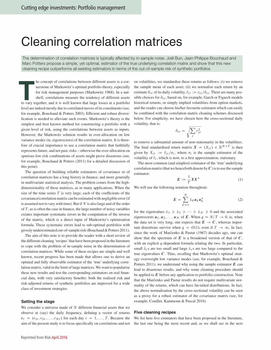
Optimal shrinkage and portfolio optimisationIt is interesting to compare the optimal shrinkage function that mapsthe empirical eigenvalue �i onto its ‘cleaned’ version �i . We showthese functions in figure 2 for the three schemes we retained, ie, lin-ear shrinkage (1), clipping (3) and RIE (5), using the same data setas in figure 1. This figure clearly reveals the difference between thethree schemes. For clipping (the red dashed line), the intermediateeigenvalues are quite well estimated but the convex shape of the opti-mal shrinkage function for larger �i s is not captured. Furthermore,the larger eigenvalues are systematically overestimated. For the linearshrinkage (the green dotted line), it is immediate from figure 2 whythis method is not optimal for any shrinkage parameters ˛ 2 Œ0; 1�

(that fixes the slope of the line).We now turn to optimal portfolio construction using the above three

cleaning schemes, with the aim of comparing the (average) realisedrisk of optimal Markowitz portfolios constructed as:

w WDO �1g

g� O �1g(14)

where g is a vector of predictions and O is the cleaned covariancematrix O

ij WD O�i O�jO� ij for any i; j 2 ŒŒ1; N ��. Note again that we

consider here returns normalised by an estimator of their volatility:Qrit D rit = O�it . This means that our tests are immune to an overallincrease or decrease of the the volatility in the out-of-period, and are




�

�

�

�

�

�

�

�


2 Comparison of the debiased RIE (10) (the blue line) with clip-ping at the edge of the Marcenko-Pastur (the red dashed line)and the linear shrinkage with ˛ D 0.5 (green dotted line)

0 1 2 3 4 50

1

2

3

4

5

ClippingLinearRIE

λ

ξ

We use the same data set as in figure 1

only sensitive to the quality of the estimator of the correlation matrixitself.

In order to ascertain the robustness of our results in different marketsituations, we consider the following four families of predictors g.� 1. The minimum variance portfolio, corresponding to gi D 1 8i 2ŒŒ1; N ��.� 2. The omniscient case, ie, when we know exactly the realisedreturns on the next out-of-sample period for each stock. This is givenby gi D N Qri;t .Tout/, where ri;t .�/ D .Pi;tC� � Pi;t /=Pi;t withPi;t the price of the i th asset at time t and Qrit D rit = O�it .� 3. Mean reversion on the return of the last day: gi D �N Qrit

8i 2 ŒŒ1; N ��.� 4. Random long-short predictors where g D N v, where v is arandom vector uniformly distributed on the unit sphere.

The normalisation factor N WDp

N is chosen to ensure wi �O.N �1/ for all i . The out-of-sample risk R2 is obtained from (13)by replacing the matrix X by the normalised return matrix QR definedby QR WD . Qrit / 2 RN �T . We report the average out-of-sample riskfor these various portfolios in table A, for the three above cleaningschemes and the three geographical zones, keeping the same value ofT (the learning period) and Tout (the out-of-sample period) as above.The linear shrinkage estimator uses a shrinkage intensity ˛ estimatedfrom the data following Ledoit & Wolf (2003) (LW). The eigenvaluesclipping procedure uses the position of the Marcenko-Pastur edge,.1Cp

q/2, to discriminate between meaningful and noisy eigenvalues.The second to last line gives the result obtained by taking the identitymatrix (total shrinkage, ˛ D 0) and the last one is obtained by takingthe uncleaned, in-sample correlation matrix (˛ D 1).

These tables reveal that (i) it is always better to use a cleaned corre-lation matrix: the out-of-sample risk without cleaning is, as expected,always higher than with any of the cleaning schemes, even with fouryears of data; and (ii) in all cases but one (minimum risk portfolioin Japan, where the LW linear shrinkage outperforms), our debiasedRIE is providing the lowest out-of-sample risk, independently of thetype of predictor used. Note that these results are statistically signif-icant everywhere, except perhaps for the minimum variance strategy

A. Annualised out-of-sample average volatility (in %) of the differentstrategies (standard errors are given in brackets)

Minimum variance portfolioUS Japan Europe


Omniscient predictorUS Japan Europe


Mean reversion predictorUS Japan Europe


Uniform predictorUS Japan Europe

RIE 1.30 (8e-4) 1.50 (1e-3) 1.23 (1e-3)Clipping MP 1.31 (8e-4) 1.55 (1e-3) 1.32 (1e-3)Linear LW 1.32 (8e-4) 1.61 (1e-3) 1.27 (1e-3)Identity 1.56 (2e-3) 1.86 (2e-3) 1.69 (2e-3)In sample 1.69 (1e-3) 2.00 (2e-3) 2.7 (0.01)

B. Annualised out-of-sample average volatility (in %) of the meanreversion strategy as a function of N with q D 0.5

USN


JapanN


EuropeN


with Japanese stocks: see the standard errors that are given betweenparenthesis in table A. Moreover, the result is robust in the dimen-sion N as indicated in table B for the mean reversion strategy. For theother strategies, some fluctuations can be observed for N D 100 butthe results are identical to those of table A for N > 200 (see Bun,Bouchaud & Potters 2016).

risk.net 57


Risk April 2016

�

�

�

�

�

�

�

�


SummaryTo summarise, we have briefly reviewed several cleaning schemesfor noisy financial correlation matrices that have been proposed inthe last 20 years. The latest one, proposed very recently in Bun &Knowles (2016) as an extension of previous work by Ledoit & Péché,is remarkably good at predicting the out-of-sample risk of individualeigenportfolios (ie, portfolios with weights given by the eigenvec-tors of the correlation matrices). This method outperforms all othermethods to date at minimising the out-of-sample (realised) risk ofvarious types of Markowitz optimal portfolios (once volatilities havebeen factored out). We are confident that this method will become astandard in the coming years; it also suggests various routes for fur-ther improvements, including modelling a genuine evolution of thecorrelation matrix itself, beyond measurement noise. �

Joël Bun is a PhD candidate at the Université Paris-Saclay andat the Léonard de Vinci Pôle Universitaire, and an analyst atCapital Fund Management in Paris. Jean-Philippe Bouchaudis chairman and chief scientist and Marc Potters is co-CEOand head of research of Capital Fund Management. We areindebted to R. Benichou, A. Beveratos, R. Chicheportiche, A.Rej, E. Sérié and G. Simon for many insightful discussions andhelp in the preparation of this work. We also acknowledge use-ful conversations with R. Couillet on robust estimators. Finally,we warmly thank A. Knowles for his contribution to this topicthat led to the paper Bun & Knowles (2016).Email: [email protected],

[email protected],[email protected].

REFERENCES

Bouchaud J-P and M Potters,2003Theory of financial risk andderivative pricing: from statisticalphysics to risk managementCambridge University Press

Bouchaud J-P and M Potters,2011Financial applications of randommatrix theory: a short reviewIn The Oxford Handbook ofRandom Matrix TheoryOxford University Press

Bun J, J-P Bouchaud andM Potters, 2016Cleaning large correlationmatrices: tools from randommatrix theoryIn preparation

Bun J and A Knowles, 2016An optimal rotational invariantestimator for general covariancematricesIn preparation

Burda Z, J Jurkiewicz andB Wacław, 2005Spectral moments of correlatedWishart matricesPhysical Review E 71(2), 026111

Couillet R, A Kammoun andF Pascal, 2016Second order statistics of robustestimators of scatter: applicationto GLRT detection for ellipticalsignalsJournal of Multivariate Analysis143, pages 249–274

El Karoui N, 2008Spectrum estimation for largedimensional covariance matricesusing random matrix theoryAnnals of Statistics 36(6),pages 2757–2790

Haff L, 1980Empirical Bayes estimation ofthe multivariate normalcovariance matrixAnnals of Statistics 8,pages 586–597

Ledoit O and S Péché, 2011Eigenvectors of some largesample covariance matrixensemblesProbability Theory and RelatedFields 151(1-2), pages 233–264

Ledoit O and M Wolf, 2003Improved estimation of thecovariance matrix of stockreturns with an application toportfolio selectionJournal of Empirical Finance10(5), pages 603–621

Ledoit O and M Wolf, 2014Nonlinear shrinkage of thecovariance matrix for portfolioselection: Markowitz meetsgoldilocksAvailable at SSRN 2383361

Markowitz HM, 1968Portfolio selection: efficientdiversification of investments,volume 16Yale University Press

Marcenko VA and LA Pastur,1967Distribution of eigenvalues forsome sets of random matricesMatematicheskii Sbornik 114(4),pages 507–536

Monasson R and D Villamaina,2015Estimating the principalcomponents of correlationmatrices from all their empiricaleigenvectorsEurophysics Letters 112(5), 50001

Pafka S and I Kondor, 2003Noisy covariance matrices andportfolio optimization IIPhysica A: Statistical Mechanicsand its Applications 319,pages 487–494

Box 1. Implementation of the debiased RIE

We present the complete procedure to construct our optimal estimatorof E mostly based on the optimal shrinkage function (7). This algorithmcan easily be implemented in any computer language that can handlecomplex numbers.

Given the eigenvalues Œ�k�NkD1

of the sample correlation matrix E

and q D N=T , we define the complex variable zk D �k � i=p

N forany k 2 ŒŒ1; N ��. Then, the cleaning scheme reads:� 1. We compute for any k 2 ŒŒ1; N ��:

�RIEk D �k

j1 � q C qzksk.zk/j2 (15)

with:

sk.zk/ D 1

N

NXj D1j ¤k

1

zk � �j

(16)

� 2. We evaluate at the same time for any k 2 ŒŒ1; N ��:

�k D �2 j1 � q C qzkgmp.zk/j2�k

(17)

where gmp.z/ is the Stieltjes transform of the (rescaled) Marcenko-Pastur density given by:

gmp.z/ D z C �2.q � 1/ �p

z � �N

pz � �C

2qz�2(18)

with:

�C D �N

�1 C p

q

1 � pq

�2

; �2 D �N

.1 � pq/2

(19)

where �N is the smallest empirical eigenvalue.� 3. Our debiased optimal RIE for any k 2 ŒŒ1; N �� reads:

O�k D(

�k�RIEk

if �k > 1

�RIEk

otherwise(20)




cleaning correlation matrices - cfm · cleaning correlation matrices the determination of...

Documents