Principal Direction Divisive Partitioning�Daniel BoleyyDepartment of Computer Science and EngineeringUniversity of Minnesota200 Union Street S.E., Rm 4-192Minneapolis, MN 55455, USAAbstractWe propose a new algorithm capable of partitioning a set of documents or othersamples based on an embedding in a high dimensional Euclidean space (i.e. in whichevery document is a vector of real numbers). The method is unusual in that it isdivisive, as opposed to agglomerative, and operates by repeatedly splitting clustersinto smaller clusters. The documents are assembled in to a matrix which is verysparse. It is this sparsity that permits the algorithm to be very e�cient. The per-formance of the method is illustrated with a set of text documents obtained from theWorld Wide Web. Some possible extensions are proposed for further investigation.1 IntroductionUnsupervised clustering of documents is a critical component for the exploration of largeunstructured document sets. As part of a larger project, the WebACE Project [16, 11], wehave developed a novel algorithm for unsupervised partitioning of a large data set whichexhibits several useful features. These features include scalability to large data sets, compet-itive performance in terms of the quality of the clusters generated, and capability of working�This research was partially supported by NSF grants CCR-9405380 and CCR-9628786.ytel: 1-612-625-3887, fax: 1-612-625-0572, e-mail: boley@cs.umn.edu1

on data sets where the number of attributes is much larger than the number of sample doc-uments. The overall WebACE project aims to create an agent that would help users explorethe World Wide Web (WWW) by carrying out the following steps:1. Starting with a seed set of user-retrieved documents, automatically classify documentsretrieved.2. Generate new WWW searches using classes discovered in step 1 or 3.3. Classify newly received documents into existing classes, or update the classi�cationstructure without user intervention.4. Repeat from step 2.A critical part of this task is a method to automatically discover structure present in a largeset of documents and to classify a new set of documents according to a previously computedset of classes. Unsupervised clustering is important because the volume of data available onthe Web is enourmous. Any classi�cation system depending on human input would quicklybe overwhelmed. On the other hand, an automatically generated classi�cation of a largecollection of documents retrieved by the agent, or retrieved by the user over several browsingsessions would be of immense value in allowing the user to easily navigate the documentcollection.The goal of this paper is to present one such algorithm which we have observed is capableof competitive performance in terms of speed, scalability, and quality of class structure found.We make a remark on the origin of the name \Principal Direction Divisive Partitioning."The words \Principal Direction" are used because the algorithm is based on the computationof the leading principal direction at each stage in the partitioning. The key component inthis algorithm that allows it to operate fast is a fast solver for this direction. This principaldirection is used to cut a cluster of documents repeatedly. The use of a distance or similaritymeasure is limited to deciding which cluster should be split next, but the similarity measureis not used to do the actual splitting.We use the word \Partitioning" to re ect the fact that we place all the documents in onecluster, so that at every stage the clusters are disjoint and their union equals the entire setof documents.The word \Divisive" comes from the following taxonomy of clustering algorithms in [17,p298] (originally from [1]): 2

1. hierarchical agglomerative clustering2. hierarchical divisive clustering3. iterative partitioning4. density search clustering5. factor analytic clustering6. clumping7. graph-theoretic clusteringOur algorithm is a hierarchical algorithm, but the overwhelming majority of existing hier-archical algorithms which treat the documents as a point in Euclidean space work \bottomup" by agglomeration. Our PDDP algorithm is \top down" or \divisive" in the sense that itstarts with all the documents in one single big cluster and proceeds to divide up the initialcluster into progressively smaller clusters.As a hierarchical divisive algorithm, the PDDP algorithm would be appropriate for thescatter/gather task of [7]. This is discussed further in Section 5.2 Related WorkExisting approaches to document clustering are generally based on either probabilistic meth-ods, or distance and similarity measures (see [9]). Distance-based methods such as k-meansanalysis, hierarchical clustering [13] and nearest-neighbor clustering [15] use a selected setof words (features) appearing in di�erent documents as the dimensions. Each such featurevector, representing a document, can be viewed as a point in this multi-dimensional space. Itwill be seen that our method also uses distance measures to a limited extent, as well as termweighting and normalization, but the algorithm's scalability allows us to avoid the necessityof removing words or reducing the dimensionality in advance.AutoClass [6] is a method using Bayesian analysis based on the probabilistic mixturemodeling [22]. Given a data set it �nds maximum parameter values for a speci�c probabilitydistribution functions of the clusters.There are a number of problems with clustering in a multi-dimensional space using tra-ditional distance- or probability-based methods. First, it is not trivial to de�ne a distancemeasure in this space. Some words are more frequent in a document than other words.3

Simple frequency of the occurrence of words is not adequate, as some documents are largerthan others. Furthermore, some words may occur frequently across documents. Techniquessuch as tfidf [19] have been proposed precisely to deal with some of these problems.Secondly, the number of all the words in all the documents can be very large. Distance-based schemes generally require the calculation of the mean of document clusters. If thedimensionality is high, then the calculated mean values may not di�er signi�cantly from onecluster to the next, especially if the initial set of clusters are poor. Hence the cluster meansmay not provide good separation. Similarly, probabilistic methods such as Bayesian classi�-cation used in AutoClass [6] do not perform well when the size of the feature space is muchlarger than the size of the sample set and the attributes are not statistically independent, asis typical of document categorization applications on the Web. It is possible to reduce thedimensionality by selecting only frequent words from each document, or to use some othermethod to extract the salient features of each document. However, the number of featurescollected using these methods still tends to be very large, and determining which featurescan be discarded without a�ecting the quality of clusters is di�cult.Latent Semantic Indexing (LSI) [2] was proposed as a method for query-based documentretrieval in which the noise present in data sets of very high dimensionality is reduced byorthogonal projection. A low rank (say, rank k � minfm;ng, where m;n are the numberof documents and words, respectively) approximation to the term frequency matrix M iscomputed using the leading k singular values and vectors of the matrix. This has the e�ectof removing the noise, while representing each document by means of a set of k \generalizedattributes." But unlike the PDDP algorithm, the singular value decomposition is appliedto M, not A = (M � weT ), where w; e are the centroid vector and the vector of all ones,respectively, de�ned in Section 3, and is used only to preprocess the data to reduce thedimensionality of its representation. In addition, computing k leading singular values andvectors is considerably more complicated and expensive than computing just one as in thePDDP Algorithm.Linear discriminant functions have been used extensively to partition samples in a testset into two classes. An example is the Fisher linear discriminant function (see e.g. [17]),typically used with a training set of samples with known \correct" classi�cations. As suchit is usually used as a tool in \supervised learning," in which a training set with previouslyknown class designations are used. An \optimal" direction is chosen on which to project4

all the samples, and a cut-point is selected using a one-dimensional Bayes rule based on theknown mean and covariance matrices for the individual classes.Previous algorithms for unsupervised clustering based on the use of one-dimensionalBayesian analysis or linear discriminants is very limited, at least to the knoweldge of thisauthor. A hint in this direction appears in [17, p500], where the repeated use of a Fisher-stylelinear discriminant is suggested, resulting in a hierarchical classi�cation. It is even suggestedthat the Karhunen Loeve transformation might lead to good directions, which would lead toan algorithm such as the one introduced in this paper. However no algorithm is given andno discussion of the speci�c structure that might result from such an algorithm is discussed.There has been some more recent work on projections and hierarchical structures fordata analysis. Bishop and Tipping [3] assemble a series of projections of the data intoa hierarchical tree structure, but for the purpose of visualizing a set of numerical data.Sch�utze and Silverstein [20] explore the e�ects on the accuracy of clustering algorithms ofvarious strategies for initial term selection, weighting, and projections. Singhal et al [21]explore the e�ect of di�erent tfidf scalings and other normalization strategies in a studythat is more systematic than that in Section 5 of this paper. Zamir et al [23] proposethe method of word intersection clustering based on a global quality function. This is ameasure of cluster cohesion which is a viable alternative to the scatter measures used in thispaper. Zamir's work is reported in the context of new fast clustering methods for web searchresults. Northern Light Search [18] also clusters results of web searches, but the speci�cs oftheir method is not included. The work reported below in Section 6 is related to other workin text �ltering and classi�cation. In [12] there is a study showing how great improvementsin accuracy can be achieved by combining several di�erent learning methods.3 Notation and Mathematical PreliminariesWe will represent column vectors with lower case bold letters, matrices with upper casebold letters, scalars with italic letters, viz. v = (v1; v2; : : : ; vn)T where n is the dimensionof v. The transpose of a matrix M is the matrix MT whose i; j-th element is �ji, where�ij denotes the i; j-th element of M. A row vector will be denoted by uT . The notatione = (1; 1; : : : ; 1)T will stand for a vector of all ones of appropriate dimension. In this paper5

we will use the Euclidean norm for vectors:kvk2 = sXj v2j ; (1)and the Frobenius norm for matrices:kMkF = sXi;j �2ij; (2)The algorithm presented in this paper will be applied to document vectors. A documentvector d = (d1; d2; : : : ; dn)T is a column vector whose i-th entry, di, is the relative frequencyof the i-th word. In this particular application, we scale the document vectors to haveEuclidean norm equal to 1, so that each entry has the numerical valuedi = TFiqPj(TFj)2 ; (3)where TFi is the number of occurences of word i in the particular document d. We refer tothe scaling (3) as \norm scaling." An alternative scaling is the tfidf scaling, de�ned usingthe recommended \nfc" alternative from [19] as follows:let ~di = 12 1 + TFimaxj(TFj)! � �log� mDFi�� , then di = ~diqPj( ~dj)2 ; (3:1)where DFi is the number of di�erent documents in which the i word appears, among alldocuments in the entire document set, and m is the total number of documents. However,this scaling results in a nonzero value for every di, and hence destroys the sparsity presentin the matrix. In addition it did not produce distinctly better clustering results, at leastin our experiments, compared to (3). The sparsity structure is critical for the speed of ouralgorithm. The \tfc" alternative of [19] would be a better choice from the sparsity point ofview.Given a collection of documents d1; : : : ;dm, the mean or centroid of the document set isw = d1 + � � �+ dmm =M � e � 1m; (4)where M = (d1; : : : ;dm) is an n � m matrix of document vectors. If w = 0, then thecovariance matrix of this set would be M �MT , since each sample is a column vector, but inthe general case the covariance matrix isC = (M�weT ) � (M�weT )T = A �AT ; (5)6

where A = (M�weT ). This matrix is symmetric and positive de�nite, so all its eigenvaluesare real and non-negative. The eigenvectors corresponding to the k largest eigenvalues arecalled the principal components or principal directions. In our algorithm, we are interestedonly in the eigenvectors of C, not the eigenvalues, so the speci�c scaling of the matrix C isnot important to our algorithm. In Section 4.2 we show how we avoid the need to computeC explicitly.4 Algorithm DescriptionThe Principal Component Divisive Partitioning algorithm operates on a sample space ofm samples in which each sample is an n-vector containing a numerical value. For clarity ofpresentation we will use the terms \document" to refer to a sample, but in fact this algorithmcan in principle be applied to samples in other domains for which the appropriate scaling maydi�er. Each document is represented by a column vector (3) of attribute values, which in thecase of actual text documents are word counts. In our experiments using web documents, wenormalized each document vector to have a Euclidean length of 1. For the purposes of ouralgorithm, the entire set of documents is represented by an n�m matrix M = (d1; : : : ;dm)whose i-th column, di, is the column vector representing the i-th document.The algorithm proceeds by separating the entire set of documents into two partitionsby using principal directions in a way that we will describe. Each of the two partitionswill be separated into two subpartitions using the same process recursively. The resultis a hierarchical structure of partitions arranged into a binary tree (the \PDDP tree") inwhich each partition is either a leaf node (meaning it has not been separated) or has beenseparated into two subpartitions forming its two children in the PDDP tree. The detailsof the algorithm we must specify are (1) what method is used to split a partition into twosubpartitions, and (2) in what order are the partitions selected to be split. The rest of thissection is devoted to �lling in this details.4.1 Splitting a PartitionA partition of p documents is represented by an n � p matrix Mp = (d1 � � � dp ) whereeach di is an n-vector representing a document. The matrixMp is a submatrix of the original7

matrixM consisting of some selection of p columns ofM, not necessarily the �rst p in the set,but we omit the extra subscripts for simplicity. The principal directions of the matrixMp arethe eigenvectors of its sample covariance matrix C. Let w =Mpe=p be the sample mean ofthe documents d1; : : : ; dp, and the covariance matrix is C = (Mp�weT )(Mp�weT )T . TheKarhunen-Loeve transformation [8] consists of projecting the columns of Mp onto the spacespanned by the leading k eigenvectors (those corresponding to the k largest eigenvalues). Theresult is a representation of the original data in k degrees of freedom instead of the original n.Besides reducing the dimensionality, the transformation often has another bene�cial e�ectof removing much noise present in the data, assuming an appropriate value of k can bechosen. In our case, we are interested in temporarily projecting each document onto thesingle leading eigenvector, which we will denote u. This leading eigenvector is called theprincipal component or principal direction. This projection is needed only to determine thesplit and is not otherwise used for any purpose. Intuitively, the leading eigenvector is chosenbecause it is the direction of maximum variance and hence is the direction in which thedocuments tend to be the most spread out.The projection of the i-th document di is given by the formula�vi = uT (di �w); (7)where � is a positive constant arising from the speci�c algorithm we use. In words, wetranslate all the documents so that their mean is at the origin, and then project the resultonto the principal direction. The values v1; : : : ; vk are used to determine the splitting forthe cluster Mp. In the simplest version of the algorithm, we split the documents strictlyaccording to the sign of the corresponding vi's. All the documents di for which vi � 0 arepartitioned into the left child, and all the documents di for which vi > 0 are put into theright child. A document coinciding exactly with the mean vector w is more or less in themiddle of the entire cloud of documents, and its projection (7) will be zero. In this case wemake the arbitrary choice to put such documents into the left child.The choice of splitting at the mean is somewhat arbitrary, but an intuitive justi�cationis the following. If there were two well separated clusters, then the mean would likely bebetween the two clusters. In real date sets, the mean might end up among one of the\natural" clusters, which would then be cut in two. But the algorithm will still succeed inseparating the elements of this cluster from neighboring clusters in a subsequent step.8

4.2 Computational ConsiderationsIn the computation of the splitting of the partition, the single most expensive part of thecomputation is the computation of the eigenvalues and eigenvectors of the covariance matrixC. When C has large dimensionality this can be a signi�cant expense. Standard o�-the-shelfmethods typically compute all the eigenvalues and eigenvectors. Even if special methods thatcompute only selected eigenvectors are used, many methods still require the computationof all the eigenvalues [10]. In addition, the covariance matrix is actually the product of amatrix and its transpose. This is exactly the situation where it is well known that accuracycan be improved by using the Singular Value Decomposition (SVD) [10]. The SVD of ann � m matrix A is the decomposition U�VT = A, where U;V are square orthogonalmatrices of dimension n � n, m � m, respectively, and � =diagf�1; : : : ; �minfm;ngg, where�1 � �2 � � � � � �minm;n � 0. The �'s are called the singular values, the columns of U arecalled the left singular vectors, and the columns of V are called the right singular vectors.An orthogonal matrix U is a square matrix satisfying UTU = I.Setting A =Mp �weT , we can show how to relate the SVD to the principal directions.We have C = AAT = (U�VT ) � (V�TUT ) = U�2UT ;where we use �2 as a shorthand for the n � n diagonal matrix diagf�21; �22; : : :g. From thisformula, it is seen that the eigenvalues of C are the squares of the singular values of A, andthe eigenvectors of C are the left singular vectors of A. The singular vectors also satisfyanother interesting relation. Let uj,vj denote the j-th column of U;V, respectively. Wehave that uTj A = uTj U�VT = �jvTj ; (8)and likewise Avj = �juj. Using our de�nition for A, we see that the projections (7) areexactly the entries in the vector �1vT1 . This means that once we have the SVD of the matrixA, we already have the projections needed to split the cluster Mp.In order to compute the projections (7), it is clear that we do not need the entire SVD ofA. We need only the leading singular vectors u1;v1, which we will denote u;v for short. Afast method for computing a partial SVD of a matrix can be constructed using the Lanczosalgorithm [10]. This algorithm takes advantage of sparsity present in the matrix Mp. Inour implementation of this algorithm, we implicitly compute the eigenvalues of AAT or9

ATA, whichever has a smaller dimension. The accuracy we obtain is quite su�cient for ourpurposes, since we need only to have the signs of (7).The Lanczos algorithm proceeds by repeatedly multiplying a vector x by the matrix Cand then orthogonalizing the result against all previous vectors in the sequence. It is thisproperty that allows us to avoid forming A or C explicitly. The matrix vector product A �vcan be computed directly from M by the formula Av = Mv �w(eTv). A similar formulaapplies to the product AT �v, and hence we can also obtain the product Cv without formingC. The Lanczos algorithm also constructs a sequence of nested tridiagonal matrices of in-creasing dimensions, computing the eigenvalues for each one, until a stopping test is satis�ed.For readers interested in the details of the Lanczos algorithm we implemented, we include afew details about the algorithm. We used no re-orthogonalization because all the spuriouseigenvalues thus introduced are in the interior of the spectrum and hence do not a�ect thecomputed value for the largest eigenvalue, which is the only one we seek. Our stopping testwas based on the observation that the eigenvalues of each tridiagonal matrix interlace thoseof the next one in the sequence. Hence the Lanczos algorithm proceeds until the largesteigenvalue stops growing, at which time we assume it has converged. Since only the largesteigenvalue is sought, a Sturm sequence method can be used to compute it fast from thelargest eigenvalue of the preceeding tridiagonal matrix, and furthermore, spurious eigenval-ues can be ignored. Once the eigenvalue is found, the generated Lanczos vectors are used tocompute the approximate corresponding eigenvector. All of these properties mentioned hereare based on the theory present in [10] and hence is not further discussed here.4.3 Overall AlgorithmWe summarize the overall algorithm used to carry out the partitioning. The basic algorithmconstructs a binary tree, the PDDP tree. Each node in the tree is a data structure whichholds the documents associated with that node, the various quantities computed from thatset of documents, and pointers to the two children nodes, if any. Table 1 lists the speci�cinformation stored in each node in the tree in our implementation. The information storedin each node consists of the documents in the cluster associated with that node (to savespace we store only the indices of the documents), the centroid (mean) vector, the leading10

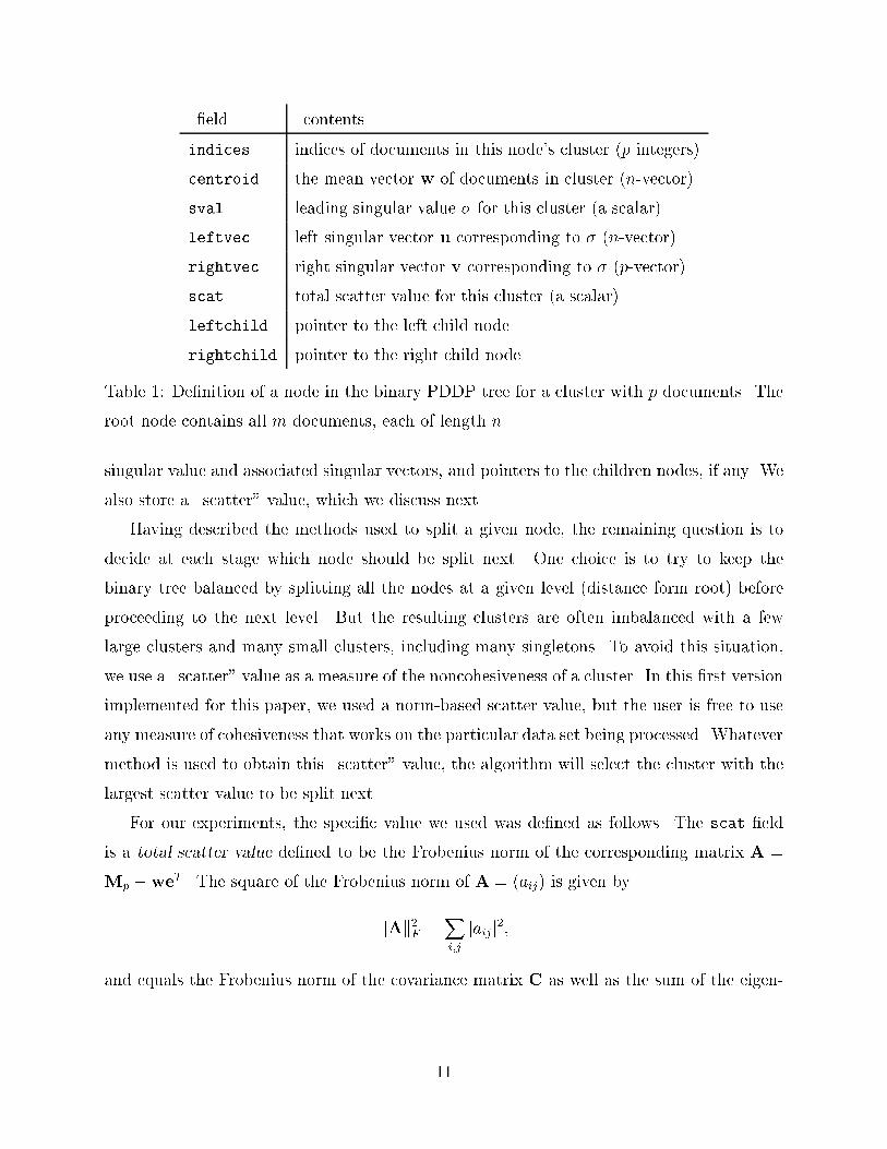
�eld contentsindices indices of documents in this node's cluster (p integers)centroid the mean vector w of documents in cluster (n-vector)sval leading singular value � for this cluster (a scalar)leftvec left singular vector u corresponding to � (n-vector)rightvec right singular vector v corresponding to � (p-vector)scat total scatter value for this cluster (a scalar)leftchild pointer to the left child noderightchild pointer to the right child nodeTable 1: De�nition of a node in the binary PDDP tree for a cluster with p documents. Theroot node contains all m documents, each of length n.singular value and associated singular vectors, and pointers to the children nodes, if any. Wealso store a \scatter" value, which we discuss next.Having described the methods used to split a given node, the remaining question is todecide at each stage which node should be split next. One choice is to try to keep thebinary tree balanced by splitting all the nodes at a given level (distance form root) beforeproceeding to the next level. But the resulting clusters are often imbalanced with a fewlarge clusters and many small clusters, including many singletons. To avoid this situation,we use a \scatter" value as a measure of the noncohesiveness of a cluster. In this �rst versionimplemented for this paper, we used a norm-based scatter value, but the user is free to useany measure of cohesiveness that works on the particular data set being processed. Whatevermethod is used to obtain this \scatter" value, the algorithm will select the cluster with thelargest scatter value to be split next.For our experiments, the speci�c value we used was de�ned as follows. The scat �eldis a total scatter value de�ned to be the Frobenius norm of the corresponding matrix A =Mp �weT . The square of the Frobenius norm of A = (aij) is given bykAk2F =Xi;j jaijj2;and equals the Frobenius norm of the covariance matrix C as well as the sum of the eigen-11

values �2i of C [10]: kAk2F = kCkF =Xi �2i :In our algorithm, the total scatter value is used to select the next cluster to split. Wechoose the cluster with the largest scatter value. The total scatter value re ects the distancebetween each document in the cluster and the overall mean of the cluster, which is a measureof the cohesiveness of the cluster. Using the total scatter value to choose the next clusterto be split usually results in clusters all having more or less similar numbers of documents.We remark that this scatter value is the only component of this algorithm that is based ona \distance" measure, and it would be just as easy to use other measures not based on a\distance" measure and appropriate for particular data sets.Having discussed all the components of our algorithm, we now summarize the overallalgorithm in Table 2. At each pass through the main loop, we select a node based on ourmeasure of \cohesiveness," obtain the mean vector and principal direction for the documentsassociated with that node, and split the documents using the mean vector and principaldirection into two children nodes. In geometric terms, we split the documents using thehyperplane normal to the principal direction passing through the mean vector.In Table 2, one can replace cmax with an alternative stopping test based on the largestscatter value present in any unsplit cluster. Indeed, in the software available in [4], we stopwhen this maximum cluster scatter falls below the scatter of the collected centroid vectors.This was the stopping test included as part of the Web agent WebACE [11] and when usingthe data from [14].The space required for the PDDP algorithm arises from three sources: the memory tostore the initial raw data matrix M, the memory needed to store the PDDP tree, andtemporary storage for the SVD computation. The space to store M is �xed. Regardingthe PDDP tree, we start with a single node, and in each step we add two new nodes tothe tree. Therefore, when �nding cmax clusters, we will have a total of 2 � cmax � 1 nodesin the tree, of which cmax are leaf nodes. Within each node, we require storage for at least2 n-vectors (centroid and leftvec), as well as space for the indices (indices) and somescalars. The remaining vector rightvec can be omitted to save space by recomputing itwhen needed using (8). In addition, leftvec and rightvec are not needed for the leafnodes, unless one would like to be able to continue the splitting process from the current12

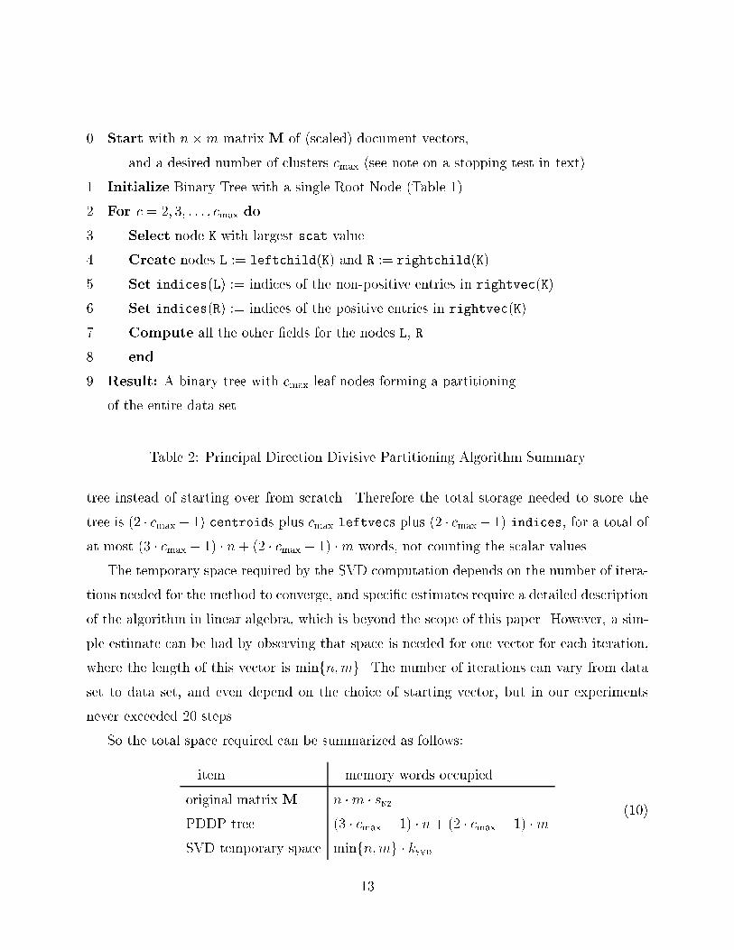
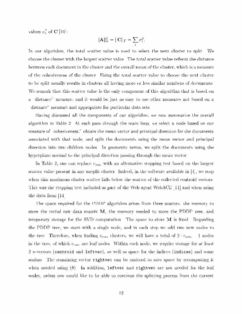
0. Start with n�m matrix M of (scaled) document vectors,and a desired number of clusters cmax (see note on a stopping test in text).1. Initialize Binary Tree with a single Root Node (Table 1).2. For c = 2; 3; : : : ; cmax do3. Select node K with largest scat value4. Create nodes L := leftchild(K) and R := rightchild(K).5. Set indices(L) := indices of the non-positive entries in rightvec(K)6. Set indices(R) := indices of the positive entries in rightvec(K)7. Compute all the other �elds for the nodes L, R.8. end.9. Result: A binary tree with cmax leaf nodes forming a partitioningof the entire data set.Table 2: Principal Direction Divisive Partitioning Algorithm Summarytree instead of starting over from scratch. Therefore the total storage needed to store thetree is (2 � cmax� 1) centroids plus cmax leftvecs plus (2 � cmax� 1) indices, for a total ofat most (3 � cmax � 1) � n+ (2 � cmax � 1) �m words, not counting the scalar values.The temporary space required by the SVD computation depends on the number of itera-tions needed for the method to converge, and speci�c estimates require a detailed descriptionof the algorithm in linear algebra, which is beyond the scope of this paper. However, a sim-ple estimate can be had by observing that space is needed for one vector for each iteration,where the length of this vector is minfn;mg. The number of iterations can vary from dataset to data set, and even depend on the choice of starting vector, but in our experimentsnever exceeded 20 steps.So the total space required can be summarized as follows:item memory words occupiedoriginal matrix M n �m � snzPDDP tree (3 � cmax � 1) � n + (2 � cmax � 1) �mSVD temporary space minfn;mg � ksvd (10)13

where snz is the fraction of entries in M that are nonzero, cmax is the number of clustersgenerated, ksvd is the number of Lanczos iterations in the SVD computation. In our appli-cation, n� m, so minfn;mg = m. In addition, typical values for snz in our examples rangefrom :04 = 4% down to :0068 = :68%.The bulk of the cost in the algorithm of Table 2 is the SVD computation in step 7.We have already mentioned that the main memory required for this step is space for ksvdm-vectors. The cost of generating each of those vectors is dominated by two matrix vectorproducts involving the matrix Mp. Taking advantage of the sparsity of M, the cost of asingle matrix vector product involving M is approximately snz �m � n. Hence the total costof the matrix vector products within the SVD step is approximately ksvdsnz � m � n. Thisis, of course, an upper bound since the later clusters contain much fewer than m documentspresent initially. Beyond the SVD computation, the equivalent of a matrix vector productis required for the centroid vector and for the scat value. So the total cost of the matrixvector products is bounded above bycmax � (2 + ksvd)snz �m � n: (11)The cost of all the rest of the computation is equivalent to lower order terms. We remark thatthis expected running time is linear in the number of documents (m), modulo the numberof iterations within the SVD computation, whereas unmodi�ed agglomeration algorithmstypically have O(m2) running time [7]. The "Buckshot" heuristic used by [7] is also an O(m)method, but depends on a random initial partition and hence is not completely deterministic.5 Experimental ResultsWe present some experimental results that show that the PDDP algorithm is e�ective, atleast as well as an agglomeration algorithm, but is much faster. We used a set of 185documents downloaded from the World Wide Web, which were then processed to obtainword counts for each document. To obtain word counts, we removed the stop words (�xedin advance), stemmed the remaining words for plurals, verb tenses, etc., and counted upthe occurences. The result was the matrix \J1" with 185 columns corresponding to the185 documents, and 10536 rows each corresponding to a word. Then further heuristics wereapplied to obtain the matrices for data sets J2 through J11. These are summarized in Table 314

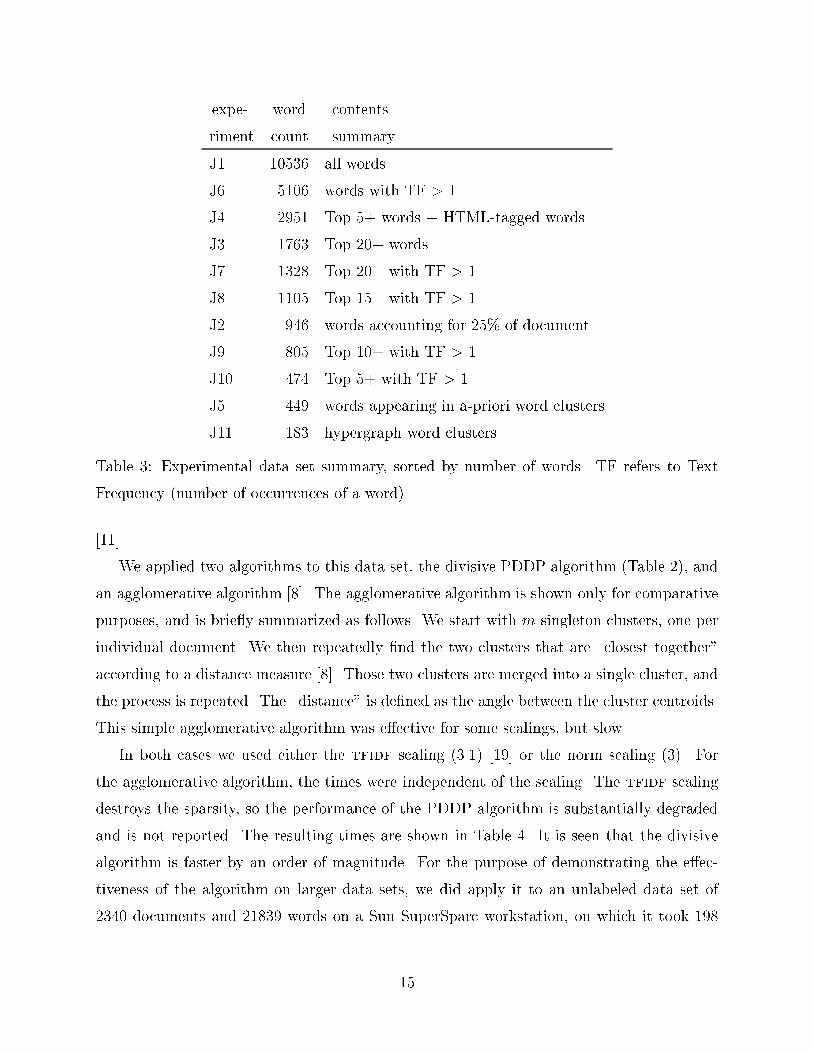
expe- word contentsriment count summaryJ1 10536 all wordsJ6 5106 words with TF > 1J4 2951 Top 5+ words + HTML-tagged wordsJ3 1763 Top 20+ wordsJ7 1328 Top 20+ with TF > 1J8 1105 Top 15+ with TF > 1J2 946 words accounting for 25% of documentJ9 805 Top 10+ with TF > 1J10 474 Top 5+ with TF > 1J5 449 words appearing in a-priori word clustersJ11 183 hypergraph word clusters.Table 3: Experimental data set summary, sorted by number of words. TF refers to TextFrequency (number of occurrences of a word).[11].We applied two algorithms to this data set, the divisive PDDP algorithm (Table 2), andan agglomerative algorithm [8]. The agglomerative algorithm is shown only for comparativepurposes, and is brie y summarized as follows. We start with m singleton clusters, one perindividual document. We then repeatedly �nd the two clusters that are \closest together"according to a distance measure [8]. Those two clusters are merged into a single cluster, andthe process is repeated. The \distance" is de�ned as the angle between the cluster centroids.This simple agglomerative algorithm was e�ective for some scalings, but slow.In both cases we used either the tfidf scaling (3.1) [19] or the norm scaling (3). Forthe agglomerative algorithm, the times were independent of the scaling. The tfidf scalingdestroys the sparsity, so the performance of the PDDP algorithm is substantially degradedand is not reported. The resulting times are shown in Table 4. It is seen that the divisivealgorithm is faster by an order of magnitude. For the purpose of demonstrating the e�ec-tiveness of the algorithm on larger data sets, we did apply it to an unlabeled data set of2340 documents and 21839 words on a Sun SuperSparc workstation, on which it took 19815

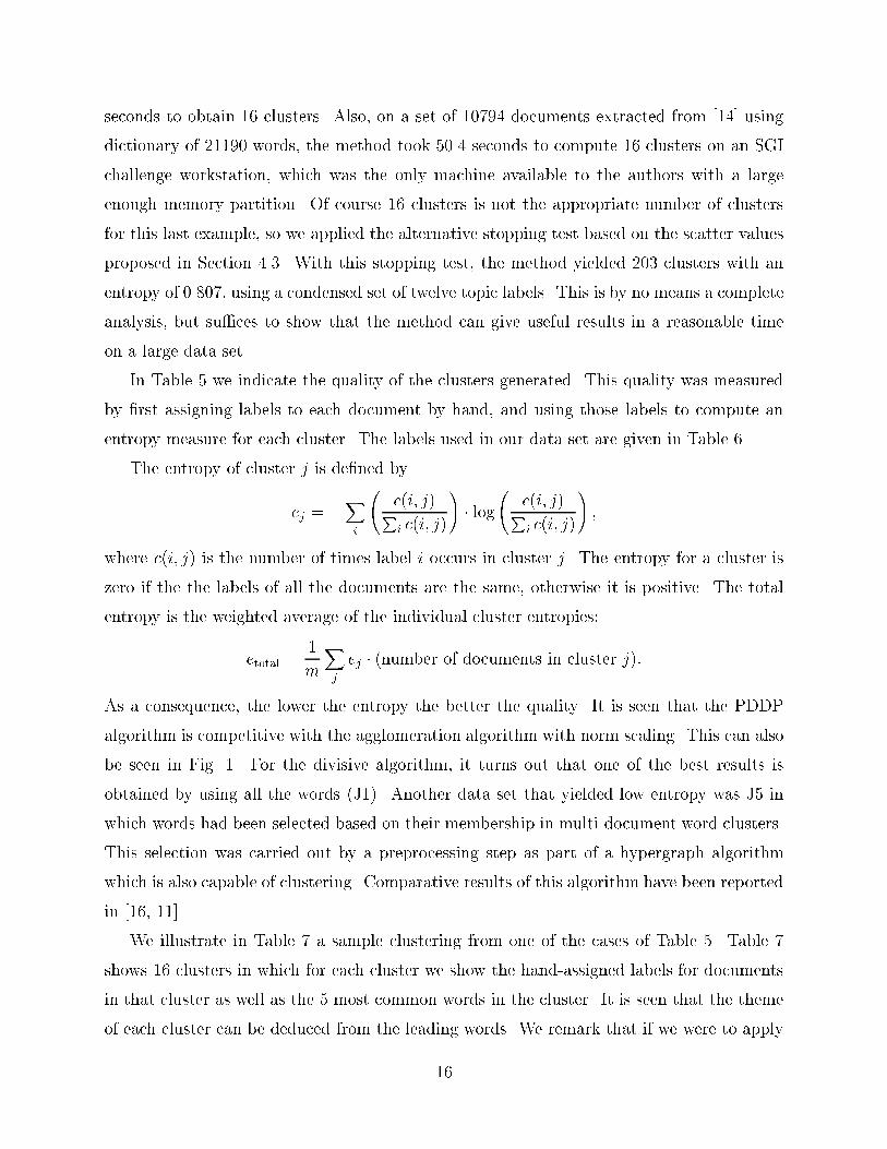
seconds to obtain 16 clusters. Also, on a set of 10794 documents extracted from [14] usingdictionary of 21190 words, the method took 50.4 seconds to compute 16 clusters on an SGIchallenge workstation, which was the only machine available to the authors with a largeenough memory partition. Of course 16 clusters is not the appropriate number of clustersfor this last example, so we applied the alternative stopping test based on the scatter valuesproposed in Section 4.3. With this stopping test, the method yielded 203 clusters with anentropy of 0.807, using a condensed set of twelve topic labels. This is by no means a completeanalysis, but su�ces to show that the method can give useful results in a reasonable timeon a large data set.In Table 5 we indicate the quality of the clusters generated. This quality was measuredby �rst assigning labels to each document by hand, and using those labels to compute anentropy measure for each cluster. The labels used in our data set are given in Table 6.The entropy of cluster j is de�ned byej = �Xi c(i; j)Pi c(i; j)! � log c(i; j)Pi c(i; j)! ;where c(i; j) is the number of times label i occurs in cluster j. The entropy for a cluster iszero if the the labels of all the documents are the same, otherwise it is positive. The totalentropy is the weighted average of the individual cluster entropies:etotal = 1mXj ej � (number of documents in cluster j):As a consequence, the lower the entropy the better the quality. It is seen that the PDDPalgorithm is competitive with the agglomeration algorithm with norm scaling. This can alsobe seen in Fig. 1. For the divisive algorithm, it turns out that one of the best results isobtained by using all the words (J1). Another data set that yielded low entropy was J5 inwhich words had been selected based on their membership in multi-document word clusters.This selection was carried out by a preprocessing step as part of a hypergraph algorithmwhich is also capable of clustering. Comparative results of this algorithm have been reportedin [16, 11].We illustrate in Table 7 a sample clustering from one of the cases of Table 5. Table 7shows 16 clusters in which for each cluster we show the hand-assigned labels for documentsin that cluster as well as the 5 most common words in the cluster. It is seen that the themeof each cluster can be deduced from the leading words. We remark that if we were to apply16

divisive algorithm agglomerative algorithmdata 8 16 32 16 32set clusters clusters clusters clusters clustersJ1 1:40 1:54 2:10 { {J6 0:39 0:44 0:50 53:15 52:57J4 0:24 0:27 0:30 29:23 29:14J3 0:15 0:17 0:20 16:54 16:48J7 0:13 0:14 0:17 11:35 11:31J8 0:21 0:23 0:25 11:31 11:23J2 0:11 0:12 0:14 7:49 7:45J9 0:10 0:11 0:14 6:19 6:15J10 0:08 0:09 0:11 3:51 3:49J5 0:11 0:13 0:16 3:38 3:35J11 0:07 0:08 0:11 1:45 1:43Table 4: Comparative times (min:sec) for divisive and agglomerative algorithms, in Matlab5 on an SGI Challenge 194 MHz processor.

17

data number of clusters:set 8 16* 32 8 16* 32 16* 32 16* 32divisive algorithm agglomerative algorithmnorm scaling tfidf scaling norm scaling tfidf scalingJ1 1.24 0.69 0.51 1.46 1.06 0.71 0.68 0.47 2.34 1.56J6 1.33 0.83 0.56 1.17 0.77 0.65 0.73 0.55 2.14 1.32J4 1.53 1.10 0.71 1.65 1.18 0.93 1.00 0.72 2.05 1.28J3 1.33 0.85 0.61 1.57 1.11 0.93 0.81 0.62 2.02 1.20J7 1.36 0.90 0.61 1.28 0.91 0.72 0.78 0.58 2.18 1.38J8 1.47 0.96 0.69 1.32 0.91 0.77 0.89 0.65 2.17 1.47J2 1.70 1.12 0.76 1.56 1.14 0.81 0.89 0.62 2.07 1.24J9 1.65 1.07 0.76 1.42 1.02 0.76 1.01 0.73 1.97 1.15J10 1.69 1.17 0.85 1.90 1.24 0.99 0.97 0.75 2.13 1.29J5 1.31 0.74 0.51 1.07 0.61 0.46 0.84 0.55 1.35 0.84J11 1.47 1.05 0.67 1.68 1.19 0.92 0.97 0.73 1.48 1.02Table 5: Entropies. Starred columns are plotted in Fig. 1. Clusters for the boxed result areshown in Table 7.

18

1 2 3 4 5 6 7 8 9 10 110

0.5

1

1.5

2

2.5

D normD tfidf

A norm

A tfidf

entropies of the 16−cluster J experiments

experiment number

entr

opy

Figure 1: Entropies for the 16-cluster experiments. Lines with dots use tfidf scaling,without dots norm scaling. Lines with dashes use agglomerative algorithm, without dashesuse divisive algorithm.19

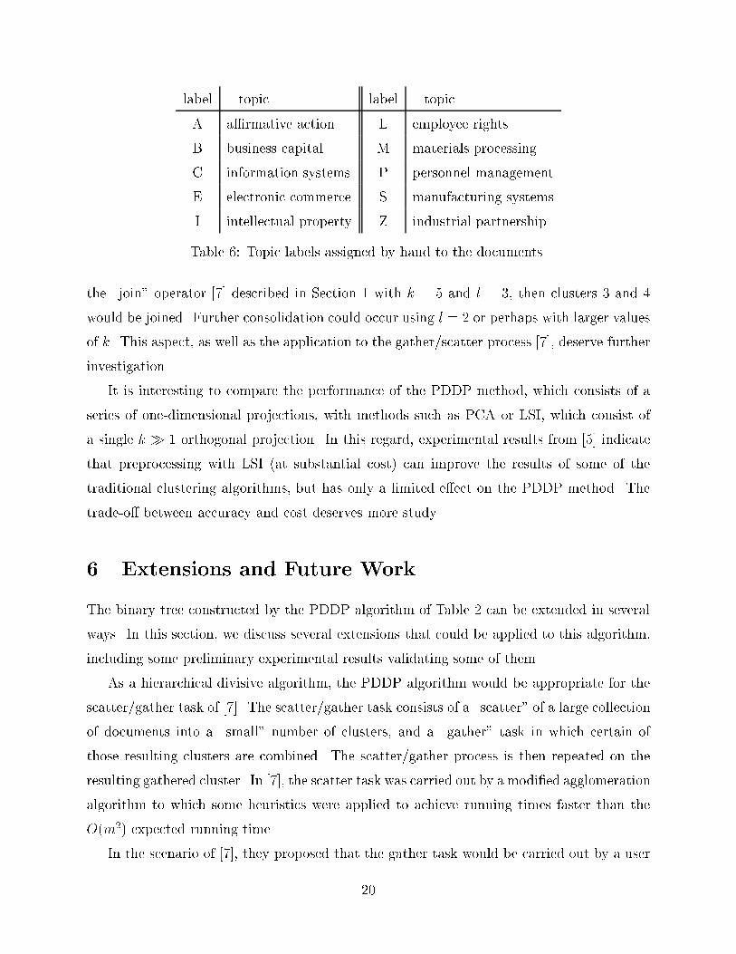
label topic label topicA a�rmative action L employee rightsB business capital M materials processingC information systems P personnel managementE electronic commerce S manufacturing systemsI intellectual property Z industrial partnershipTable 6: Topic labels assigned by hand to the documents.the \join" operator [7] described in Section 1 with k = 5 and l = 3, then clusters 3 and 4would be joined. Further consolidation could occur using l = 2 or perhaps with larger valuesof k. This aspect, as well as the application to the gather/scatter process [7], deserve furtherinvestigation.It is interesting to compare the performance of the PDDP method, which consists of aseries of one-dimensional projections, with methods such as PCA or LSI, which consist ofa single k � 1 orthogonal projection. In this regard, experimental results from [5] indicatethat preprocessing with LSI (at substantial cost) can improve the results of some of thetraditional clustering algorithms, but has only a limited e�ect on the PDDP method. Thetrade-o� between accuracy and cost deserves more study.6 Extensions and Future WorkThe binary tree constructed by the PDDP algorithm of Table 2 can be extended in severalways. In this section, we discuss several extensions that could be applied to this algorithm,including some preliminary experimental results validating some of them.As a hierarchical divisive algorithm, the PDDP algorithm would be appropriate for thescatter/gather task of [7]. The scatter/gather task consists of a \scatter" of a large collectionof documents into a \small" number of clusters, and a \gather" task in which certain ofthose resulting clusters are combined. The scatter/gather process is then repeated on theresulting gathered cluster. In [7], the scatter task was carried out by a modi�ed agglomerationalgorithm to which some heuristics were applied to achieve running times faster than theO(m2) expected running time.In the scenario of [7], they proposed that the gather task would be carried out by a user20

1: A A A A A A A A A A A A A Aa�rm action people discrimin act2: A A A A A A L L Pemploy action applic minor a�rm3: B B B B B B B B B B Zbusi capit develop fund loan4: B B B B B B B B B M Pbusi capit �nanc fund �nanci5: C C C C C C C C C C C Sinform system manag servic technologi6: C C C M S S Z Z Z Z Z Zindustri research inform system engin7: C C M S S S S S S S S S S Ssystem manufactur inform integr develop8: C E E E E E E E E E E E E E E Eelectron internet commerc busi web9: C E E E I I I I I I I L Mcopyright right web internet advertis10: C M Z Z Z Z Z Z Zindustri partnership inform program contact11: E P P P P Zpublic manag personnel hb depart12: I I I I I I I I I I I Ipatent intellectu properti copyright inform13: L L L L L L L L L L L L L Pemploye union employ court right14: M M M M M M M M M M Mmateri process engin manufactur develop15: M S S S S Z Z Z Ztechnologi manufactur develop industri product16: P P P P P P P P P P P Ppersonnel manag servic job federTable 7: Labels and 5 most common words (after stemming) within each of 16 clusterscomputed by PDDP algorithm on the J1 data set.21

who would be given information on the nature of the documents in each cluster, for examplethe most frequent words or sample document titles. They also proposed a \join" operatoron clusters that could be used to automate the gather task. The \join" operator is de�nedin terms of the list of the k most common words in the �rst cluster, for some given k. If atleast l words from this list (for some given l � k) also appear among the k most commonwords in the second cluster, then the two clusters are joined.6.1 Classi�cation of New DocumentsThe simplest extension to the PDDP algorithm of Table 2 is to classify a new set of docu-ments according to the clusters from an original document set by using the original binaryPDDP tree. For simplicity, we discuss the task of classifying a single new document d usingthe PDDP tree constructed from an initial set of documents. The PDDP algorithm yieldsa collection of clusters, and the classi�cation task is to select the cluster most closely asso-ciated with the new document. Since the initial set of documents have been separated bya sequence of hyperplanes, the resulting clusters occupy regions in n-dimensional Euclideanspace bounded by the hyperplanes (polytope regions), and each document from the initialset has been placed into one of these polytope regions. The classi�cation task for the newdocument d can be viewed as determining in which polytope region it lies. One can thenview d as most closely associated with the documents from the initial set occupying thesame polytope region.The classi�cation task then proceeds as follows. From the root node of the tree we retrievethe mean vector, w and principal direction vector u corresponding to the entire initial setof documents. These two vectors de�ne a hyperplane which was used to split the initial setof documents, but the same hyperplane actually cuts the entire space. Hence we can assignthe new document d to the left child or the right child of the root depending on which sideof this hyperplane it lies. Speci�cally, apply the formula (7) to the new document d�v = uT (d�w); (12)using the retrieved vectors w;u. If the resulting value v is positive, the d is assigned to theroot's right child, otherwise it is assigned to the left child. This process is then repeated toassign d to either the left or right child at the next level, until ultimately d percolates downto a leaf node. The resulting algorithm is summarized in Table 8.22

0. Start with PDDP binary tree and a new document d.1. Initialize node := root node of binary tree.2. While node is not a leaf node do3. Retrieve w := centroid(node) and u := leftvec(node).4. Compute v := uT (d�w).5. If v > 0 then Set node := rightchild(node)6. else Set node := leftchild(node)8. end.9. Result: node contains the leaf node to which d was assigned.Table 8: A Classi�cation Algorithm: classify a new document d by �nding associated clusterof old documents.To test this classi�cation method, we conducted a preliminary experiment of attemptingto classify half the J1 document set using a PDDP tree constructed using the other half ofthe documents. We selected the documents so that both document sets had representativesof every topic label. We used the method of Table 2 on the �rst half of the document setto construct a new PDDP tree with 16 leaf nodes, then we used the method of Table 8to classify the remaining documents, so that we end up with a set of 16 clusters, eachcontaining documents from both halves of the original document set. The resulting entropyof the combined result (i.e. all the documents) was 0.756, only slightly degraded from theoriginal entropy of 0.69 obtained when all 185 documents are processed together.Of course, the purpose of this process is to classify documents from di�erent sources, butwe have not yet addressed issues of merging such documents into a common data set. Inparticular, if the word dictionary used for the two sets of documents are di�erent, then someparadigm must be used to select the words to be kept in the combined set. This is especiallycritical if the words used in each individual set have been pruned as in experiments J2-J11.By adding documents, the combined set of words may not be the same as what one wouldobtain if all the documents were processed together. This will all be reserved for futureinvestigation. 23

6.2 Classi�cation UpdatesWe address the problem of updating the PDDP tree when new documents have arrived. Onecan consider just the leaf nodes which represent the actual clusters and treat this simplyas a problem of updating the existing clusters. One may use the Classi�cation algorithmto assign all the new documents to existing clusters and then use one of the many existingupdating algorithms on the set of clusters (see, e.g., [8, p201 or p225] or [7]). The drawbackof such an approach is that clusters created by another updating method no longer have anyconnection with the PDDP tree.A possible approach for rapidly constructing a new PDDP tree is outlined as follows. Theobvious idea is simply combine the entire new set of documents with the initial set and runthe PDDP algorithm from scratch. Of course this does not constitute updating, since thecost will be more than the cost of the PDDP algorithm on either data set alone. However wecan save substantial costs by replacing the initial set of documents with the set of centroidvectors extracted from the tree. We then combine the centroid vectors with the set of newdocuments to form a set not much larger than the new set of documents. The success of thisapproach depends on the capability of the centroids alone to capture the structure of theoriginal document set. So we show the results of an experiment that attempts to measurethis capability.To illustrate and support this idea, we considered the following experiment. We treatedhalf the documents in the J1 data set as the \old" documents, and half as the \new"documents. We extracted the 31 centroid vectors obtained during the construction of 16clusters for the \old" documents, combined them with the \new" documents, and constructeda new PDDP tree using this combined set. To test the quality of the result, we used theresulting tree to classify the entire J1 data set and found the entropy to be 0.728 comparedto 0.69 (the boxed value in Table 5) when all the documents are clustered together. Theresult is sensitive to scaling of the centroid vectors, for example to account for the fact thatthe centroids are being used to represent a larger set of documents. For example, scaling thecentroids by 1.1 without modifying the algorithm yields an entropy for the entire J1 set of.572, but the best scaling appropriate in similar situations is not known. This indicates thatthe centroids do capture a signi�cant part of the structure of the \old" documents.By using \new" documents from the same source as the \old" documents, we automat-24

ically are using the same set of words for both sets. In general, however, documents fromdi�erent sources will most likely be based on di�erent word sets, so one is faced with theproblem of merging two di�erent word sets. This aspect, and many other aspects about thisupdate strategy remain to be investigated.7 ConclusionsWe have proposed a new algorithm for the unsupervised partitioning of documents thatis based on the use of principal directions (also known as principal components), and is\divisive" in nature, in contrast to almost all other algorithms based on the embeddingof documents in high dimensional Euclidean space. Though based on an embedding in ahigh dimensional Euclidean space, no use of a distance function is made except for the verylimited use of deciding which cluster to split next. We have illustrated its performance usinga set of documents obtained from the World Wide Web and compared it to a traditionalagglomerative algorithm. The use of this algorithm is not limited to text documents, butcan be applied to any sample space embeddable in Euclidean space. We have also indicatedsome possible extensions and uses for this algorithm and pointed out directions for futurework.AcknowledgmentsThe author would like to acknowledge Robert Gross for carrying out some of the experimentsreported in this paper, and all the other members of the WebACE team: M. Gini, S. Han,K. Hastings, G. Karypis, V. Kumar, B. Mobasher, and J. Moore, for bringing this problemto the attention of the author, for retrieving the documents, and for computing and savingthe matrices of word counts for various experimental data sets used in this paper.References[1] M. R. Anderberg. Cluster Analysis for Applications. Academic Press, 1973.25

[2] M. W. Berry, S. T. Dumais, and G. W. O'Brien. Using linear algebra for intelligentinformation retrieval. SIAM Review, 37:573{595, 1995.[3] C. Bishop and M. Tipping. A hierarchical latent variable model for data visualization.IEEE Trans. Patt. Anal. Mach. Intell., 20(3):281{293, 1998.[4] D. Boley. Experimental PDDP Software. http://www.cs.umn.edu/�boley/PDDP.html,1998.[5] D. Boley, M. Gini, R. Gross, E.-H. Han, K. Hastings, G. Karypis, V. Kumar,B. Mobasher, and J. Moore. Document categorization and query generation on theworld wide web using WebACE. AI Review, 1998. to appear.[6] P. Cheeseman and J. Stutz. Bayesian classi�cation (AutoClass): Theory and results.In U. Fayyad, G. Piatetsky-Shapiro, P. Smyth, and R. Uthurusamy, editors, Advancesin Knowledge Discovery and Data Mining, pages 153{180. AAAI/MIT Press, 1996.[7] D. Cutting, D. Karger, J. Pedersen, and J. Tukey. Scatter/gather: a cluster-basedapproach to browsing large document collections. In 15th Ann Int ACM SIGIR Confer-ence on Research and Development in Information Retrieval (SIGIR'92), pages 318{329,1992.[8] R. O. Duda and P. E. Hart. Pattern Classi�cation and Scene Analysis. John Wiley &Sons, 1973.[9] W. B. Frakes and R. Baeza-Yates. Information Retrieval Data Structures and Algo-rithms. Prentice Hall, Englewood Cli�s, NJ, 1992.[10] G. H. Golub and C. F. Van Loan. Matrix Computations. Johns Hopkins Univ. Press,3rd edition, 1996.[11] S. Han, D. Boley, M. Gini, R. Gross, K. Hastings, G. Karypis, V. Kumar, B. Mobasher,and J. Moore. WebACE: A web agent for document categorization and exploration.Univ. of Minn. Comp. Sci. report TR 97-049, 1997.[12] D. Hull, J. Pederson, and H. Sch�utze. Method combination for document �ltering. InACM SIGIR 96, pages 279{287, 1996. 26

[13] A. Jain and R. C. Dubes. Algorithms for Clustering Data. Prentice Hall, 1988.[14] D. Lewis. Reuters-21578. http://www.research.att.com/�lewis, 1997.[15] S. Lu and K. Fu. A sentence-to-sentence clustering procedure for pattern analysis. IEEETransactions on Systems, Man and Cybernetics, 8:381{389, 1978.[16] J. Moore, S. Han, D. Boley, M. Gini, R. Gross, K. Hastings, G. Karypis, V. Kumar,and B. Mobasher. Web page categorization and feature selection using association ruleand principal component clustering. In 7th Workshop on Information Technologies andSystems (WITS '97), Dec. 1997. Atlanta.[17] M. Nadler and E. P. Smith. Pattern Recognition Engineering. Wiley, 1993.[18] Northern Light, 1998. http://www.nlsearch.com.[19] G. Salton and C. Buckley. Term-weighting approaches in automatic text retrieval.Information Processing and Management, 24(5):513{523, 1988.[20] H. Sch�utwe and C. Silverstein. Projections for e�cient document clustering. In ACMSIGIR 97, pages 74{81, 1997.[21] A. Singhal, C. Buckley, and M. Mitra. Pivoted document length normalization. In ACMSIGIR 96, pages 21{29, 1996.[22] D. Titterington, A. Smith, and U. Makov. Statistical Analysis of Finite Mixture Distri-butions. John Wiley & Sons, 1985.[23] O. Zamir, O. Etzioni, O. Madani, and R. Karp. Fast and intuitive clustering of webdocuments. In KDD 97, 1997.

27