click here full article a new rainfall model based on the ...espace.inrs.ca/9498/1/p1587.pdf ·...

A new rainfall model based on the Neyman-Scott

process using cubic copulas

G. Evin1 and A.-C. Favre1

Received 20 March 2007; revised 24 September 2007; accepted 5 November 2007; published 29 March 2008.

[1] A classical way to model rainfall is to use a Poisson process. Authors generallyemployed cluster of rectangular pulses to reproduce the hierarchical structure ofrainfall storms. Although independence between cell intensity and duration turned out tobe a nonrealistic assumption, only a few models link these variables. In this paper, aNeyman-Scott cluster process considering dependence between cell depth and duration isdeveloped. We introduce this link with a cubic copula. Copulas are multivariatedistributions modeling the dependence structure between variables, preserving themarginal distributions. Thanks to this flexibility, we are able to introduce a global conceptof dependence between cell depth and duration. We derive the aggregated moments(first-, second-, and third-order moments) from the new model for several families ofpolynomial copulas and perform an application on Belgium and American data.

Citation: Evin, G., and A.-C. Favre (2008), A new rainfall model based on the Neyman-Scott process using cubic copulas,

Water Resour. Res., 44, W03433, doi:10.1029/2007WR006054.

1. Introduction

[2] A stochastic model of the rainfall process at a pointdescribes the behavior of precipitation in time. In thispaper we focus on a specific type of model which usesPoisson-cluster processes to represent rainfall, namely theNeyman-Scott Rectangular Pulses Model (NSRPM). Manyapplications have proved the effectiveness of such modelsfor the analysis of data collected on a short timescale, e.g.,hourly [see Rodriguez-Iturbe et al., 1987b; Cowpertwait etal., 1996; Onof et al., 2000]. Two well-known rectangularpulses models have been extensively used: the Bartlett-Lewis and the Neyman-Scott models. For a detailed reviewof developments with this type of rainfall model, see Onofet al. [2000]. In order to easily derive the theoreticalmoments of the aggregated intensity of rainfall (mean,variance, autocovariance), most models assume an inde-pendent relation between rain cell intensity and duration.[3] This hypothesis is questionable for many reasons. The

model would be more flexible without this condition andmore suitable to adequately represent the temporal structureof rainfall. Furthermore, the link between storm durationand intensity is often significantly negative [De Michele andSalvadori, 2003]. Kim and Kavvas [2006] call the hypoth-esis of independence into question and review some devel-opments [see Cordova and Rodriguez-Iturbe, 1985; Singhand Singh, 1991; Bacchi et al., 1994; Kurothe et al., 1997;Goel et al., 2000] where correlated rain cells arrive accord-ing to a simple Poisson process (i.e., without clustering).The authors cite some bivariate exponential distributions[Gumbel’s [1960] type I, Downton [1970]] which are usedto consider negative or positive correlation between rainfallintensity and duration. However, these representations do

not consider clusters and appear to be limited. Without thecluster approach, the Poisson-based model has difficulties torepresent more than one timescale [Rodriguez-Iturbe et al.,1987a]. Kim and Kavvas [2006] develop a NSRPM whichconsiders positive and negative correlations with a Gum-bel’s Type-II bivariate distribution. Kakou [1997] includes adependence in the conditional mean within the Neyman-Scott model. First- and second-order moments are derivedand proportions of dry periods seem to be adequatelyreproduced at all timescales [see Onof et al., 2000]. In ourcase, a cubic copula links cell intensity and duration. Thisglobal structure of dependence in our model includes as aspecial case the Gumbel’s Type-II distribution. In fact, thelatter is composed of exponential margins and a dependencestructure consisting of the Farlie-Gumbel-Morgenstern cop-ula family (or FGM) discussed by Morgenstern [1956],Gumbel [1958], and Farlie [1960]. The use of cubic copulasis innovative in itself if we consider the scarce applicationswith this class of copulas. Thus we develop a more generalNSRPM and derive first-, second-, and third-order momentswhich enable us to fit the model with the generalized methodof moments. The paper is divided into four more sections asfollows. In section 2 the basic theory concerning the copulasand the class of cubic copulas is presented, while section 3develops the Neyman-Scott model including dependencebetween rain cell intensity and duration. Aggregatedmoments are derived up to the third order. Two applicationsare performed in section 4, and section 5 concludes.

2. Copula Theory

2.1. Copula Definition

[4] Copulas are extremely useful to solve problems thatinvolve modeling the dependence between several randomvariables. In finance, they can be applied to derivativepricing, portfolio management, the estimation of risk meas-ures (e.g., Value at Risk), risk aggregation, credit modelling

1Chaire en hydrologie statistique, Centre Eau, Terre et Environnement,Institut National de la Recherche Scientifique, Quebec, Quebec, Canada.

Copyright 2008 by the American Geophysical Union.0043-1397/08/2007WR006054$09.00

W03433

WATER RESOURCES RESEARCH, VOL. 44, W03433, doi:10.1029/2007WR006054, 2008ClickHere

for

FullArticle

1 of 18

http://dx.doi.org/10.1029/2007WR006054

[see Embrechts et al., 2002; Cherubini et al., 2004]. We alsoobserve numerous applications in actuarial science [Freesand Valdez, 1998]. Recently, copulas appeared in hydrology[e.g., De Michele and Salvadori, 2003; Favre et al., 2004a;Grimaldi and Serinaldi, 2006; Genest and Favre, 2007;Renard and Lang, 2007]. The copula representation enablesus to separate the dependence structure from the marginalbehavior. For a detailed review of the theory of copulas, theauthors refer to the monograph by Joe [1997] and Nelsen[2006].[5] For the sake of simplicity, we concentrate on the

bivariate case. One representation theorem from Sklar[1959] highlights the interest of copulas in dependencemodeling. Any joint cumulative distribution function(c.d.f.) H(x, y) of any pair (X, Y) of random variables maybe written in the form

H x; yð Þ ¼ C F xð Þ;G yð Þf g; x; y 2 R ð1Þ

where the copula C describes the dependence between therandom variables X and Y. Hence Sklar’s theorem impliesthat for multivariate distribution functions the univariatemargins and the dependence structure (represented by acopula) can be separated. Furthermore, Sklar [1959] showedthat in the case of continuous distributions F and G, C isuniquely determined.[6] As is highlighted by Genest and Favre [2007], a

judicious choice to measure dependence is to use nonpara-metric measures. Two coefficients, commonly used to thisend, are Spearman’s rho r and Kendall’s tau t. Here r and tare expressible in terms of the copula and are given by

r ¼ 12

Z0;1½ �2

C u; vð Þdvdu 3;

t ¼ 4

Z0;1½ �2

Cðu; vÞdC u; vð Þ 1:

We say that a copula C is ‘‘symmetric’’ if C(u, v) = C(v, u)for all (u, v) in [0, 1]2.[7] In our model, the copula C links cell depth and

lifetime. The use of a copula increases the complexity ofthe NSRPM. Consequently, the problem of fitting has to betaken into account to choose the form of the copula. There isno consensus over the view of copulas as being the optimalsolution to model dependencies, as illustrated by the recentand heated discussion initiated by Mikosch [2006] andfollowed by numerous authors [see, e.g., Genest andRemillard, 2006; Joe, 2006; Embrechts, 2006]. In our case,the idea of using cubic copulas is motivated by the need tohave algebraic expressions for the theoretical moments. Thechoice of the bivariate distribution on cell intensity andduration is very limited and nontrivial distributions arenecessaries to have both supple dependence structures andalgebraically tractable expressions.[8] Because of the difficulty in obtaining a suitable like-

lihood function [see, e.g., Chandler and Onof, 2005, p. 11],the generalized method of moments is the simplest way toperform the fitting of the NSRPM.With this method, the first-and second-order moments of the aggregated process must berelated to themodel parameters. The successive steps to reachin order to derive the moments limit the choice of distribu-tions to be used. Exponential families are usually employedto characterize the different random variables (see section 3),

e.g., exponential distribution, gamma distribution. Otherstype of distributions appear to increase the complexity. Inparticular, we tried to derive the moments with numerousbivariate distributions presented by Hutchinson and Lai[1990]. The expressions to be resolved appear to be intrac-table. Consequently, we study bivariate distributions on cellintensity and duration composed of products of exponentials,i.e., exponential margins with cubic copulas.

2.2. Cubic Copulas

[9] The following results are provided by QuesadaMolina and Rodrıguez Lallena [1995] and Nelsen et al.[1997]. The use of quadratic copulas with exponentialmargins is a priori a judicious choice of bivariate distribu-tions on cell intensity and duration. The aggregatedmoments can be computed and afterwards the method ofmoments can be applied. However, the only copula familywith quadratic sections in both u and v is the FGM copulawhich leads to the Gumbel type-II distribution as introducedin the NSRPM by Kim and Kavvas [2006]. With this copulafamily, the degree of dependence is restricted to [2/9;2/9]for Kendall’s tau. That is why Nelsen et al. [1997] introducecopulas with cubic sections and prove that these copulasincrease the dependence degrees compared to copulas withquadratic sections. As far as we know, this class of copulashas never been used in hydrology.[10] FollowingNelsenet al. [1997], letSdenote theunionof

the points in the square [1, 2] [2, 1] and the points in andon theellipse {(u,v)2 R

2,u2uv+v23u+3v=0}.Copulaswith cubic sections in both u and v are defined by

C u; vð Þ ¼ uvþ uv 1 uð Þ 1 vð Þ A1v 1 uð Þ½þ A2 1 vð Þ 1 uð Þ þ B1uvþ B2u 1 vð Þ� ð2Þ

where A1, A2, B1, B2 are real constants such that the points(A2, A1), (B1, B2),(B1, A1), and (A2, B2) all lie in S. The maintheoremsrelated tocubiccopulasare reported inAppendixA1.Several properties can be obtained from this representationof a cubic copula. Nelsen et al. [1997] proved that if acopula C is defined as in (2), we then have:

r ¼ A1 þ A2 þ B1 þ B2ð Þ=12

and

t ¼ A1 þ A2 þ B1 þ B2ð Þ=18þ A2B1 A1B2ð Þ=450: ð3Þ

If C has cubic sections in both u and v, then jrj ffiffiffi3

p/3.

Simple calculations lead us to find that we also have

jtj ffiffiffiffiffiffiffiffiffiffiffiffiffiffiffiffiffiffiffiffiffiffiffiffiffiffiffiffiffiffiffiffi494

ffiffiffiffiffi19

p 2053

p/25. The proof is given in

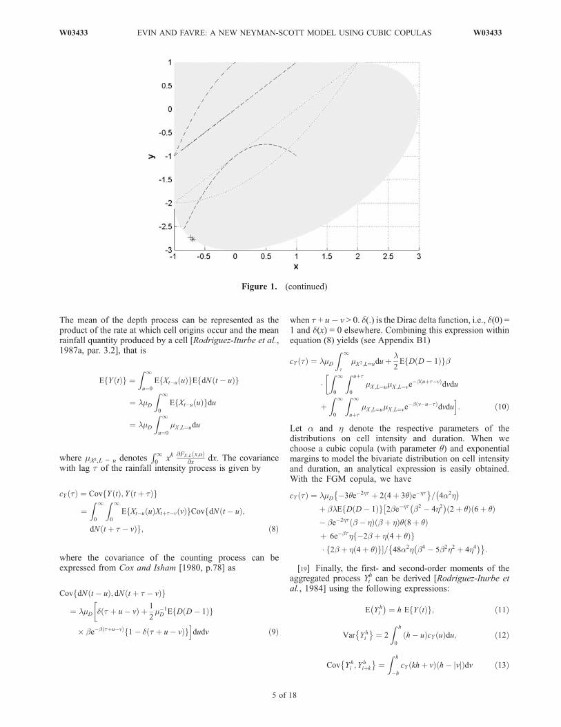
Appendix A2. Moreover, C is symmetric if and only ifA1 = B2. Numerous subfamilies may be built. When A1 =A2 = B1 = B2 = q, we obtain the special case of the Farlie-Gumbel-Morgenstern (FGM) copula defined by C(u, v) = u v{1 + q(1 u)(1 v)}. We present several of these familiesin Table 1 and in Appendix A1. The degrees ofdependence they are able to reproduce are reported inTable 2. The graph of the parameter space covered in S foreach cubic copula is given in Figure 1.[11] Families of cubic copulas with one parameter are

easy to obtain. The dependence between cell intensity andduration being probably negative, we developed the follow-ing copulas in order to attain minimum negative values forthe degree of dependence. The cubic copulas alreadydescribed by Nelsen et al. [1997] (i.e., the Sarmanov, Frank

2 of 18

W03433 EVIN AND FAVRE: A NEW NEYMAN-SCOTT MODEL USING CUBIC COPULAS W03433

cubic, and Plackett cubic families) are introduced inAppendix A1.2.2.1. AMH Cubic[12] We derive the second-order approximation to the

Ali-Mikhail-Haq (AMH) family of copulas [see Ali et al.,1978] given by

C u; vð Þ ¼ uv

1 q 1 uð Þ 1 vð Þ

for q 2 [1, 1]. This family is symmetric and includes theindependence case for q = 0.2.2.2. Sym1[13] A copula with cubic sections must respect the con-

ditions defined in Theorem A.2 (Appendix A1). We candefine a one-parameter cubic family of copulas by takingA2 =B1 = q 2 [1, 2] and A1 = B2 = q2 3 in such a way that(q, q2 3) lies in [1, 2] [2, 1]. This family issymmetric and covers a large interval of dependence butdoes not include the independence as a special case.2.2.3. Sym2[14] Let A2 = B1 = q 2 [1, 3] and let A1 =

B2 =q3

ffiffiffiffiffiffiffiffiffiffiffiffiffiffiffi9þ6q3q2

p2

. The points (A2, A1), (B1, B2), (B1, A1)

and (A2, B2) all lie in S and describe the elliptical contour of Sfrom the point [1, 2] to the point [3, 0]. This family issymmetric and attains minimum values for both r and t.2.2.4. Sym3[15] The point in S attaining the minimum value for r is

[1 ffiffiffi3

p, 1

ffiffiffi3

p]. If we consider a linear relation between

A2 = B1 and A1 = B2 passing through this point and the point[0, 0], we obtain a family that is symmetric, having linearrelations in every parameter, containing independence andattaining the minimum value for r.2.2.5. Asym1-Asym3[16] Asymmetric families are easily obtained as soon as

A1 6¼ B2. The family Asym1 maintains a quadratic relationin q and attains a large interval of dependence.

3. Neyman-Scott Model

3.1. Model Structure

[17] The same notation as Rodriguez-Iturbe et al. [1987a]is used, except for the number of cells which we denote byD in order to avoid confusion with the copula C. Supposethe arrival times of storm origins occur as a Poisson processwith rate l. A random number D of cells is associated witheach storm origin and follows a geometric distribution withmean mD. The cell origins are independently separated fromthe storm origin by distances which are exponentially

distributed with parameter b. Let a rectangular pulse beassociated with each cell origin, representing rainfall cell.Cell intensity is denoted by X and cell duration is denotedby L. The total intensity at time t, Y(t), is the summation ofthe intensities of cells alive at time t. Let Xtu(u) represent-ing the rainfall intensity at time t due to a cell with startingtime t-u. Let us consider process Y(t) defined by

Y tð Þ ¼Z 1

u¼0

Xtu uð ÞdN t uð Þ

where dN(t u) = 1 if a cell has origin at time tu and 0 ifnot. We have [see Cox and Isham, 1980] E{dN(t u)} =Var{dN(t u)} = lmDdu. Cell intensity and duration aretraditionally linked by the following definition of Xtu(u)

Xtu uð Þ ¼ X with probability F LðuÞ ¼ ehu

0 with probability FLðuÞ ¼ 1 ehu

�ð4Þ

where the cell duration is exponentially distributed withparameter h. We want the cell intensity and duration to bedependent. When a link exists between X and L, relation (4)does not hold anymore. We wish to obtain the distributionof cell intensity X with L > u that we denote FX,L. We use acopula function C to express joint distribution of X and L.We have

FX ;L x; uð Þ ¼ Pr X x; L > uð Þ¼ Pr X xð Þ Pr X x; L uð Þ¼ FX xð Þ C FX xð Þ; FL uð Þf g: ð5Þ

At this point, it is important to underline that relation (5)does not limit the choice of the bivariate distribution on cellintensity and duration. Any bivariate distribution can beexpressed with a bivariate copula and marginal distributionsaccording to Sklar’s theorem. However, it appears thatclassical bivariate distributions make very complex andeven impossible the derivation of the aggregated moments.The use of cubic copulas and exponential margins is anelegant way to obtain a flexible class of bivariatedistributions and for which aggregated moments are easilyderivable.

3.2. First- and Second-Order Moments

[18] Let Yih be the aggregated rainfall depth in the ith time

interval of length h, so that

Yhi ¼

Z ih

i1ð ÞhY tð Þdt:

Table 1. Families of One-Parameter Copulas With Cubic Sections

in u and v

Name A1 A2 B1 B2 q 2

Sarmanov q(35q) q(3 + 5q) q(3 + 5q) q(35q) [ffiffiffi7

p/5,

ffiffiffi7

p/5]

Frank cubic 3q(1q) 3q(1 + q) 3q(1 + q) 3q(1-q) [ffiffiffi3

p/3,

ffiffiffi3

p/3]

Plackett cubic q(1-q) q q q(1-q) [1,2]AMH cubic q q(1+q) q q [1,1]Sym1 q2–3 q q q2–3 [1,2]Sym2 q3

ffiffiffiffiffiffiffiffiffiffiffiffi9þ6q3q2

p2

q q q3ffiffiffiffiffiffiffiffiffiffiffiffi9þ6q3q2

p2

[1,3]

Sym3 (2+ffiffiffi3

p)q q q (2+

ffiffiffi3

p)q [1

ffiffiffi3

p,2

ffiffiffi3

p]

Asym1 q2 q1 q1 q2/32 [0,3]Asym2 q(1q)1 q q q [0.8525,1]Asym3 q(1q)+1 q q q [1,0]

Table 2. Degrees of Dependence for Families of One-Parameter

Copulas With Cubic Sections in u and v

Name r 2 t 2

Sarmanov [0.5292,0.5292] [0.3725,0.3725]Frank cubic [0.5774,0.5774] [0.4003,0.4003]Plackett cubic [0.5,0.1667] [0.34,0.1134]AMH cubic [0.25,0.4167] [0.1688,0.28]Sym1 [0.5416,0.5] [0.3778,0.34]Sym2 [0.5774,0.5] [0.4006,0.3533]Sym3 [0.5774,0.2113] [0.4003,0.1388]Asym1 [0.5,0.5] [0.34,0.34]Asym2 [0.428,0.1667] [0.2886,0.1155]Asym3 [0.3333,0.0834] [0.2222,0.0556]

W03433 EVIN AND FAVRE: A NEW NEYMAN-SCOTT MODEL USING CUBIC COPULAS

3 of 18

W03433

The mth moment is expressed by

E Yhi

� �m� �¼

Z h

0

Z h

0

. . .

Z h

0

E Y t1ð ÞY t2ð Þ . . . Y tmð Þf gdt1dt2 . . . dtm

¼ m!

Z h

0

Z h

t1

. . .

Z h

tm1

E Y t1ð ÞY t2ð Þ . . . Y tmð Þf g

� dt1dt2 . . . dtm: ð6Þ

Properties of point processes include the independencebetween point process generation dN(tmum) and cellintensity distribution Xtmum

(um). We then write:

E Y t1ð ÞY t2ð Þ . . . Y tmð Þf g

¼Z 1

u1¼0

Z 1

u2¼0

. . .

Z 1

um¼0

E Xt1u1 u1ð ÞXt2u2 u2ð Þ . . .Xtmum umð Þf g

E dN t1 u1ð ÞdN t2 u2ð Þ . . . dN tm umð Þf g: ð7Þ

Figure 1. Graph of (A2, A1),(B1, B2), (B1, A1), (A2, B2) in S (grey surface) for each cubic copula. Thepoints referring to the minimum values for the Kendall’s tau and the Spearman’s rho are represented byan asterisk and a plus symbol, respectively. Shown are (a) Sarmanov (dotted line), Frank cubic (dashedline), Plackett cubic (dash-dot line); (b) AMH cubic (dotted line), Sym1 (dashed line), Sym2 (dash-dotline), Sym3 (plain line); and (c) Asym1 (dotted line), Asym2 (dashed line), Sym3 (dash-dot line).

4 of 18


The mean of the depth process can be represented as theproduct of the rate at which cell origins occur and the meanrainfall quantity produced by a cell [Rodriguez-Iturbe et al.,1987a, par. 3.2], that is

E Y tð Þf g ¼Z 1

u¼0

E Xtu uð Þf gE dN t uð Þf g

¼ lmD

Z 1

0

E Xtu uð Þf gdu

¼ lmD

Z 1

u¼0

mX ;L¼udu

where mXk,L = u denotesR10

xk@FX ;L x;uð Þ

@x dx. The covariancewith lag t of the rainfall intensity process is given by

cY tð Þ ¼ Cov Y tð Þ; Y t þ tð Þf g

¼Z 1

0

Z 1

0

E Xtu uð ÞXtþtv vð Þf gCov dN t uð Þ;f

dN t þ t vð Þg; ð8Þ

where the covariance of the counting process can beexpressed from Cox and Isham [1980, p.78] as

Cov dN t uð Þ; dN t þ t vð Þf g

¼ lmD d t þ u vð Þ þ 1

2m1D E D D 1ð Þf g

beb tþuvð Þ 1 d t þ u vð Þf gidudv ð9Þ

when t + u v > 0. d(.) is the Dirac delta function, i.e., d(0) =1 and d(x) = 0 elsewhere. Combining this expression withinequation (8) yields (see Appendix B1)

cY tð Þ ¼ lmD

Z 1

tmX 2;L¼uduþ

l2E D D 1ð Þf gb

�Z 1

0

Z uþt

0

mX ;L¼umX ;L¼veb uþtvð Þ

dvdu

þZ 1

0

Z 1

uþtmX ;L¼umX ;L¼ve

b vutð Þdvdui: ð10Þ

Let a and h denote the respective parameters of thedistributions on cell intensity and duration. When wechoose a cubic copula (with parameter q) and exponentialmargins to model the bivariate distribution on cell intensityand duration, an analytical expression is easily obtained.With the FGM copula, we have

cY tð Þ ¼ lmD 3qe2ht þ 2 4þ 3qð Þeht� �= 4a2h� �

þ blE D D 1ð Þf g 2beht b2 4h2� �

2þ qð Þ 6þ qð Þ�

be2ht b hð Þ b þ hð Þq 8þ qð Þþ 6ebth 2b þ h 4þ qð Þf g� 2b þ h 4þ qð Þf g�= 48a2h b4 5b2h2 þ 4h4

� �� :

[19] Finally, the first- and second-order moments of theaggregated process Yi

h can be derived [Rodriguez-Iturbe etal., 1984] using the following expressions:

E Yhi

� �¼ h E Y tð Þf g; ð11Þ

Var Yhi

� �¼ 2

Z h

0

h uð ÞcY uð Þdu; ð12Þ

Cov Yhi ; Y

hiþk

� �¼

Z h

h

cY khþ vð Þ h jvjð Þdv ð13Þ

Figure 1. (continued)


5 of 18

W03433

where k is an integer representing the lag of theautocovariance function. For the FGM copula and expo-nential margins, simple expressions can be found:

E Yhi

� �¼ hlmD 4þ qð Þ

4a h;

Var Yhi

� �¼ lmD 3qþ 8ehh 4þ 3qð Þ

�þ e2hh 32 21qþ 2hh 16þ 9qð Þf g�= 8a2e2hhh3

� �:

þ lE D D 1ð Þf g 8b3 b2 4h2� �

ehh þ hh 1� ��

� 2þ qð Þ 6þ qð Þ b3 b hð Þ b þ hð Þ� e2hh þ 2hh 1� �

q 8þ qð Þ þ 24h3 ebh þ bh 1� �

� h2 4þ qð Þ24b2n oi

= 96a2h3 b5 5b3h2 þ 4bh4� ��

;

Cov Yhi ; Y

hiþk

� �¼ lmD 3 e2hh 1

� �2qþ 8ehh 1þkð Þ ehh 1

� �2n� 4þ 3qð Þg= 16a2e2hh 1þkð Þh3

� � lE D D 1ð Þf g 8b3e bþhð Þh 1þkð Þ ehh 1

� �2h� b2 4h2� �

2þ qð Þ 6þ qð Þ

þ b3ebh 1þkð Þ e2hh 1� �2

b hð Þ b þ hð Þq 8þ qð Þ

þ 24e2hh 1þkð Þ ebh 1� �2

h3

� 2bf h 4þ qð Þg 2b þ h 4þ qð Þf g�

= 192a2e bþ2hð Þh 1þkð Þh3 b5 5b3h2 þ 4bh4� �n o

:

3.3. Third-Order Moment

[20] Following Cowpertwait [1998], we derived expres-sion of the third-order moment in the case of a dependencebetween cell depth and lifetime. The third-order momentgives information about the asymmetry of a distribution.According to Cowpertwait [1998] and Onof [2003], thereproduction of extremes is greatly improved when thethird-order moment is included in the fitting procedure.To evaluate the third-order moment for the Neyman-Scottprocess, consider expression (7) with m = 3. Let t1 < t2 < t3denote the locations of three cell origins. The expectation ofthe counting process is derived in [Cowpertwait 1998,equation (2.7)]:

E dN t1ð ÞdN t2ð ÞdN t3ð Þf g

¼ l3m3Ddt1dt2dt3 þ

1

2l2bmDE D2 D

� �� eb t3t1ð Þ þ eb t3t2ð Þ þ eb t2t1ð Þn o

dt1dt2dt3

þ 1

3lb2E D2 D

� �D 2ð Þ

� �eb t3þt22t1ð Þdt1dt2dt3

þ � dt1dt2dt3ð Þ ð14Þ

where t1 < t2 < t3. Now, we need to express E{Xt1u1(u1)

Xt2u2(u2)Xt3u3

(u3)}. We have to consider different cases(for example, t1 u1 = t2 u2 in order to take into account thecase where Xt1u1

and Xt2u2refer to the same cell). Hence

E Xt1u1 u1ð ÞXt2u2 u2ð ÞXt3u3 u3ð Þf g

¼

mX 3;L¼u1þt3t1when t1 u1 ¼ t2 u2 ¼ t3 u3

mX ;L¼u1mX 2 ;L¼u2þt3t2

when u3 ¼ u2 þ t3 t2; u2 6¼ u1 þ t2 t1mX ;L¼u2

mX 2;L¼u1þt3t1when u3 ¼ u1 þ t3 t1; u2 6¼ u1 þ t2 t1

mX ;L¼u3mX 2;L¼u1þt2t1

when u2 ¼ u1 þ t2 t1; u3 6¼ u1 þ t3 t1mX ;L¼u1

mX ;L¼u2mX ;L¼u3

when t1 u1 6¼ t2 u2 6¼ t3 u3

8>>>><>>>>:

[21] Details of these computations are exposed inAppendix B2. With the FGM copula and exponentialmargins, the expression of the third (central) moment is

xh ¼ E Yhi E Yh

i

� �� 3h i

¼ 3lmD 21e2hh 1þ hhð Þqþ 24ehh�� 2þ hhð Þ 8þ 7qð Þþ3 128þ 64hh 105qþ 49hhqð Þg= 16a3h4� �

þ blE D D 1ð Þf gf h; b; q; hð Þf g

= 384a3e bþ4hð Þhh4 b5 5b3h2 þ 4bh4� �2n o

þ lE D D 1ð Þ D 2ð Þf gg h;b; q; hð Þf g

= 1280a3be2 bþ2hð Þh b 2hð Þ2 b hð Þ2h4 b þ hð Þ 2b þ hð Þn

� b þ 2hð Þ b þ 3hð Þ b þ 4hð Þg ð15Þ

where f (h, b, q, h) and g(h, b, q, h) are defined inAppendix B3.[22] When q = 0 for the FGM copula, we have C(u, v) = u

v which corresponds to the case of independence betweencell intensity and duration. For q = 0, equation (15) isconsistent with the one obtained by Cowpertwait [1998].General formulas for the aggregated moments (except thethird moment whose expression is too cumbersome) usingcubic copulas can be found in Appendix B4.

3.4. Probability of Dry Period

[23] The expression for the probability of an intervalof given length h to be dry is useful in fitting models.Cowpertwait [1991] derived this expression in the casewhere the rain cells are distributed according to a Poissondistribution. Favre [2001] gives this expression when thenumber of cells D is distributed according to a geometricdistribution:

PD hð Þ ¼ exp lhð Þ exp bhð Þ 1 mDð Þ þ mDf gl

b 1mDð Þ

exp lZ 1

0

pt hð Þdt� �

; ð16Þ

where

pt hð Þ¼ mD exp b t þ hð Þf g b hð Þ þ h exp btð Þ b exp htð Þ½ �mD1ð Þ exp b tþhð Þf gðbhÞþh exp btð Þb exp htð Þ½ �þhb

:

[24] Since the sum involved in expression (16) cannot becomputed algebraically, it requires a numerical integrationof

R10{1 pt (h)}dt.

4. Model Application

4.1. Data Description

[25] We state that the NSRPM is significantly improvedwhen dependence is included between cell intensity andduration. In this section a large simulation analysis isperformed using two data sets. Another successful applica-tion can be found in the work of Evin and Favre [2006].The first one is provided by the rainfall station at Uccle,Belgium. Rainfall data used was collected by the RoyalMeteorological Institute of Belgium. Hourly recorded rain-fall depth are made available for a period of 28 years, from1968 to 1995. The second series of hourly rainfall is anextract of the CPC Hourly U. S. Precipitation data provided

6 of 18


by the National Oceanic and Atmospheric Administration/Office of Oceanic and Atmospheric Research/Earth SystemResearch Laboratory-Physical Sciences Division (NOAA/OAR/ESRL PSD), Boulder, Colorado, USA (available fromtheir Web site at http://www.cdc.noaa.gov/cdc/data.cpc\_hour.html, accessible on 25 September 2007). NOAA’sClimate Prediction Center (CPC) provides hourly U. S.precipitation. Stations were gridded into 2.0 2.5 boxesthat extended over the region, 140�W–60�W, 20�N–60�Nusing a modified Cressman Scheme. In this paper, wepresent the application of the NSRPM on the point withcoordinates 95�W–48�N, situated in the Lower Red Lake(Minnesota). For this data set, 50 years of observations areavailable from 1949 to 1998. In order to satisfy the temporalhomogeneity with respect to rainfall characteristics, theNeyman-Scott model is usually applied on a monthly basis.Therefore without loss of generality, only results on Juneand February data are shown in this paper for the Belgianand American data, respectively. June and February wereselected to be representative months for summer and winter,respectively. The NSRPM is thus applied on two differentclimates, Uccle having an oceanic climate whereas theLower Red Lake is typical of a humid continental climate.

4.2. Models Considered

[26] We apply the modified NSRPM on these data setsusing the copula families described in Table 1. To avoidoverloaded figures and tables, we report the results for onlyfour families, namely FGM, Sym1, Sym2, and Asym1. It

must be noticed that several families were giving verysimilar results. Marginal distributions for cell duration andintensity are exponential. Thus we obtain a three-parameterbivariate distribution to characterize the behavior of cellintensity and duration. We bring to mind that the FGMcopula with exponential margins corresponds to the Gum-bel’s Type-II distribution. Thus this specific model willallow a comparison of performance between the differentmodels considered and the one developed by Kim andKavvas [2006] who apply a Gumbel’s Type-II distribution.[27] To allow a fair comparison of performance according

to the number of parameters between the classical modeland those including a dependence, we apply a gammadistribution with two parameters on cell intensity in thecase of independence, so that the cell intensity X hasprobability density function ag xg1 eax/G(g), x � 0. Wealso investigate the case of a Pareto distribution withprobability density function gag/(a + x)(g+1), x � 0 oncell intensity, where a is the scale parameter and g is theshape parameter. The classical case of a simple exponen-tial distribution on cell intensity is also presented.[28] The last type of models considered is the ‘‘Depen-

dent Depth-Duration Model’’ examined by Kakou [1997].This model conserves the storm and cell arrival rates alongwith cell duration. The cell intensity X has an exponentialform. The dependence structure between cell intensity andduration is introduced through a mean cell intensity depend-ing on L, that is E(XjL) = g(L). The exponential distribution

Table 3. Estimates of the NSRPM Parameters F at Uccle, the Dependence Degree (Kendall’s tau t and Pearson’s rho r), and the Value ofthe Objective Function O(F)

l h b mD a g t q f c r O(F)

Dist. on Cell Int.Ind. Exponential 0.0191 2.41 0.100 4.63 0.34 0 1.56e-002Ind. Gamma 0.0183 2.48 0.116 8.72 0.25 0.40 0 4.08e-003Ind. Pareto 0.0191 2.34 0.117 6.86 8.59 5.45 0 1.33e-004

Copula FamilyFGM 0.0192 2.26 0.099 4.47 0.32 0.08 0.35 1.47e-002Sym1 0.0192 2.54 0.115 6.30 0.31 0.32 0.25 4.80e-004Sym2 0.0192 2.59 0.115 6.43 0.31 –0.31 0.33 4.08e-004Asym1 0.0193 2.39 0.105 5.01 0.30 0.19 0.82 6.58e-003

DD ModelDD1 0.0191 2.41 0.100 4.63 2.94 0.00 0.00 1.56e-002DD2 0.0173 6.00 0.151 22.75 4.93 0.03 0.58 1.51e-002

Table 4. Estimates of the NSRPM Parameters F at the Lower Red Lake, the Dependence Degree (Kendall’s tau t and Pearson’s rho r),and the Value of the Objective Function O(F)

l h b mD a g t q f c r O(F)

Dist. on Cell Int.Ind. Exponential 0.0052 7.77 0.086 8.59 0.46 0 1.81e-003Ind. Gamma 0.0053 8.01 0.088 10.25 0.40 0.74 0 8.96e-004Ind. Pareto 0.0053 8.16 0.089 10.05 18.62 10.74 0 2.17e-004

Copula FamilyFGM 0.0052 7.27 0.087 8.20 0.41 0.12 0.53 1.02e-003Sym1 0.0053 9.19 0.090 11.27 0.48 0.12 0.98 4.80e-004Sym2 0.0053 9.41 0.090 11.97 0.49 0.14 1.35 6.89e-004Asym1 0.0053 8.48 0.089 9.75 0.42 0.14 1.05 1.53e-004

DD ModelDD1 0.0052 7.78 0.086 8.60 2.16 0.00 0.00 1.81e-003DD2 0.0053 9.75 0.089 14.18 13.62 2.00 0.47 1.92e-003


7 of 18

W03433

for the cell duration, L, with parameter h, say, is stillretained. Two versions of g(L) are considered: f ecL and fLecL, where f and c are nonnegative scalars. We shall referto these models as the DD1 and the DD2 model, respec-tively. In the DD1 model the variables X and L are alwaysnegatively correlated, with correlation function

zz þ 1

ffiffiffiffiffiffiffiffiffiffiffiffiffiffiffiffiffiffiffiffiffiffiffiffiffiffi2z þ 1

2z2 þ 2z þ 1

s

where z = c/h [Kakou, 1997]. With the DD2 model, thecorrelation function between rain cell intensity and duration

is

1 zz þ 1

ffiffiffiffiffiffiffiffiffiffiffiffiffiffiffiffiffiffiffiffiffiffiffiffiffiffiffiffiffiffiffiffiffiffiffiffiffiffiffiffiffiffi2z þ 1ð Þ3

4 z þ 1ð Þ4 2z þ 1ð Þ3

s

4.3. Parameter Estimation

[29] We apply the method of moments described byRodriguez-Iturbe et al. [1987a]. The functions are highlynonlinear in the parameters so that an exact solution is notavailable. Let F denotes the set of parameters. A closedsolution can be obtained by minimizing O:

Table 5. Observed and Estimated Properties at Ucclea

Mean Probability of No Rain Variance

Correlation

Lag-1 Lag-2 Lag-3

Level of Aggregation: 1 hObserved 0.107 0.881 0.339 0.395 0.269 0.176Ind. Exp. 0.108(0.105;0.111) 0.903(0.901;0.905) 0.37(0.36;0.39) 0.357 0.126 0.096Ind. Gamma 0.104(0.101;0.107) 0.864(0.861;0.866) 0.35(0.34;0.37) 0.376 0.154 0.122Ind. Pareto 0.108(0.105;0.111) 0.876(0.873;0.879) 0.34(0.32;0.35) 0.394 0.165 0.130FGM 0.109(0.105;0.111) 0.904(0.902;0.906) 0.37(0.36;0.39) 0.359 0.129 0.098Sym1 0.108(0.106;0.112) 0.884(0.881;0.886) 0.34(0.32;0.36) 0.391 0.160 0.125Sym2 0.108(0.105;0.111) 0.883(0.880;0.885) 0.34(0.32;0.36) 0.391 0.159 0.125Asym1 0.109(0.106;0.112) 0.897(0.895;0.899) 0.36(0.34;0.38) 0.369 0.139 0.107DD1 0.108(0.105;0.111) 0.903(0.901;0.905) 0.37(0.36;0.39) 0.358 0.127 0.097DD2 0.106(0.103;0.109) 0.825(0.822;0.829) 0.33(0.31;0.35) 0.377 0.211 0.180




aThe properties used in the estimation procedure are indicated in bold font.

8 of 18


O Fð Þ ¼Xpi¼1

1Mi

Mi

� �2

; ð17Þ

where Mi is a moment or autocovariance function of theNeyman-Scott model given by equations (6) and (11)–(13).It could also be the dry probability at a given scale withtheoretical expression given by (16). Here p is the numberof moments included in the procedure. The ratios Mi

Mibetween theoretical expression and observed values haveto be close to 1. The use of these ratios ensures that largenumerical values do not dominate the fitting procedure.[30] It is common to fit models using some combination

of means, variances, autocorrelations and proportions of dryintervals, at timescales ranging from 1 to 24 h. For a six-

parameter model, six theoretical expressions are sufficientto constrain the optimization problem. However, as sug-gested by Cowpertwait et al. [1996], a larger set ofmoments guarantees that the model at least fit these prop-erties. We choose hourly mean, hourly variance, hourlyautocovariance at lag-1, daily variance, daily autocovar-iance at lag-1, the third-order moment at an hourly scale,and the probability of dry period at an hourly and a dailyscale (thus we obtain p = 8). Cowpertwait [1998] indicates agood fit of extremes with the insertion of the third-ordermoment in the estimation procedure. The minimization of Ois not an easy task and must be achieved numerically.Numerous investigations show that the obtained estimatesare highly sensitive to the starting point of the search[Calenda and Napolitano, 1999]. The optimization proce-

Table 6. Observed and Estimated Properties at the Lower Red Lakea

Mean Probability of No Rain Variance

Correlation

Lag-1 Lag-2 Lag-3





aThe properties used in the estimation procedure are indicated in bold font.


9 of 18

W03433

dure is derived from the algorithm developed by Chandlerand Onof [2005] and can be summarized as follows:[31] 1. A solution in the five dimensional space is

provided by the generalized method of moments developedby Favre et al. [2004b] in the case of the classical NSRPMwith five parameters. This method uses an algebraic com-putation reducing the number of parameters estimated byminimization. Two parameters are obtained by minimiza-tion while the three others can be directly computed.[32] 2. A starting value for the parameters l, b, h, mD, a

are obtained in the first step. The sixth parameter was fixedsuch that it corresponds to the classical NSRPM. Theoptimization procedure constrains the parameter space insome realistic regions: 0.00001 < l < 0.1(h1); 0.0001 < b <0.99 (h1); 0.01 < h < 200 (h1); 1 < mD < 500; 0.01 < a <1000. By restraining the parameters between these bounds,we ensure that the estimates do not get into physicallyunrealistic parameter spaces. A subjective choice is neces-sary to set these bounds. Nevertheless, the bounds are wideand experience shows that parameters always lie in a smallsubspace of this feasible region [Cowpertwait, 1998]. A firstset of parameters are estimated by minimizing expression(17) using a sequential quadratic programming (SQP)

method [Fletcher, 2001]. This specific set of parameters isduplicated 100 times to provide a primary set of identicalsolutions.[33] 3. Repeat steps 4 to 7 several times (e.g., five times).[34] 4. Perform 50 constrained optimizations. The starting

points are generated via random perturbations about theparameter set identified above. The random perturbation istaken from a beta distribution on the current bounds (thebounds are defined in step 2 and evolute in step 6).[35] 5. Discard any parameter sets for which the objective

function exceeds 10O50, where O50 is the 50th smallest ofthe objective function values found in step 4.[36] 6. Bounds evolute according to the best parameter sets

found so far (i.e., those minimizing the objective function). Ifthe best sets are close, bounds are narrowed. If they are closeto an existing boundary, bounds are loosened.[37] 7. Keep only the 50 best parameter sets. The overall

best set is taken as a starting point for future optimizations.[38] This algorithm has the first advantage to stride an

important subset of the parameter space with the adaptivebounds and the random starting points. His second strengthis to avoid failure of minimization algorithm. This couldhappen when poor starting values are given, the objective

Figure 2. Monthly 1-day maxima at Uccle. X-axis gives the return period in years represented on aGumbel scale. Solid line with plus symbol represents observed maxima. Dotted lines represent the mean(with o) and a 0.95 confidence interval of simulated maxima obtained from 1000 simulations of 100 years.

10 of 18


function becoming too flat. The obtained estimates arepresented in Tables 3 and 4.[39] For both applications, the estimated parameters re-

lated to the point process, i.e., l and b, are quite stable. Theparameter related to the number of cells mD has an importantvariation according to the model. It points the identifiabilityproblem of the NSRPM [Chandler and Onof, 2005]. Thevalue of the shape parameter of the gamma distribution (g =0.4 at Uccle and g = 0.74 at the Lower Red Lake) indicatesthat the introduction of one extra parameter for the bivariatedistribution on cell intensity and duration allows a moreheavy-tailed distribution for cell intensity. With the FGMcopula, the dependence degree obtained is weak (t = 0.08at Uccle and t = 0.12 at the Lower Red Lake). It isimportant to bear in mind that when t = 0, this model isequivalent to the classical model with independent expo-nential margins. The DD1 model is equivalent to theclassical NSRPM for both applications (c = 0), while theDD2 model exhibits a positive correlation between cellintensity and duration. It is quite interesting to note thatKendall’s tau between the rain cell duration and intensity isnegative for the copula-based models and does not attain thelower bounds indicated in Table 2.

[40] We now consider more specifically the estimates atUccle (see Table 3). The independent Pareto, Sym1, andSym2 models achieve smaller objective values than theother models. The objective function values give an overallmeasure of model fit, it thus indicates that these modelsoutperform the other models on this application. On thecontrary, the DD1 and DD2 models seem to have difficul-ties to fit the observations. The same holds for the estimatesat the Lower Red Lake, except that the Asym1 modelclearly minimizes the objective function. The dependencedegree (see Table 4) is almost the same for all the copula-based models. Thus the value of the objective function isminimized thanks to the dependence structure (and not bythe increase of the dependence degree).

4.4. Model Performances

[41] For each type of bivariate distribution on cell inten-sity and duration, 1000 series of hourly rainfall are gener-ated, each sequence containing 100 months of data.Analysis of the variability of the series gives us an indica-tion of uncertainty.[42] Tables 5 and 6 give the fitting properties of the

different models at Uccle and at the Lower Red Lake,

Figure 3. Monthly 1-hour maxima at Uccle. X-axis gives the return period in years represented on aGumbel scale. Solid line with plus symbol represents observed maxima. Dotted lines represent the mean(with o) and a 0.95 confidence interval of simulated maxima obtained from 1000 simulations of 100 years.


11 of 18

W03433

respectively. For the mean, the probability of dry period andthe variance, we indicate a 0.95 empirical confidenceinterval in brackets, obtained from the 1000 simulations.The properties used in the estimation procedure are indi-cated in bold font. The method of moments ensures thatthese properties give good fitted values. As noticed in theprevious section, objective values (see Tables 3 and 4)indicate the ability of each model to reproduce the observedstatistics. The objective values are directly linked to thedifferences between the observed and simulated propertiesof rainfall. At Uccle, the FGM model does not improve theclassical NSRPM in this sense, mainly because of the weakdependence degree (t = 0.08) while the Ind. Pareto,Sym1, and Sym2 models clearly outperform the othermodels. The Asym1 model is the best model at the LowerRed Lake for this criterion. At Uccle, the variance at a6 h and 12 h level of aggregation seems to be slightlyunderestimated for all models, which is not true at theLower Red Lake. The probability of dry periods areadequately reproduced at the same scales. At a daily scalethe lag two and lag three correlations are clearly too weak inan absolute sense for both applications.

[43] It is important to notice that it is difficult to make anycomparison of observed and modeled dependence degrees.The NSRPM is a conceptual model where cells are inob-servable and an observed measure of dependence betweencell intensity and duration is impossible to obtain. Let tC bethe dependence degree between cell intensity and durationand tS the dependence degree between the storm durationand mean intensity. The relation between tC and tS is verycomplex for several reasons. First, the parameters mD, h andb jointly influence tS via a clustering effect, that is to saywhen cells are superposed and aggregated. Furthermore, thefact that we only observe rainfall intensity on discrete timeintervals attenuates tC. This point is illustrated in the workof Rodriguez-Iturbe et al. [1987b] and is called the smooth-ing effect. Finally, the need of a method to extract thestorms from the observed data is an additive noise. Thechoice of a dry period to separate different storms [see, e.g.,De Michele and Salvadori, 2003] is a source of subjectivity.[44] As pointed out by Onof et al. [2000], one main

weakness of the classical NSRPM is the reproduction ofextremes. Nonetheless, the ability of the model to reproduceextremes is a primary aspect in a risk approach. Synthetic

Figure 4. Monthly 1-day maxima at the Lower Red Lake. X-axis gives the return period in yearsrepresented on a Gumbel scale. Solid line with plus symbol represents observed maxima. Dotted linesrepresent the mean (with o) and a 0.95 confidence interval of simulated maxima obtained from 1000simulations of 100 years.

12 of 18


series provide monthly maxima at daily and hourly scales,which are represented on Figures 2–5. The X-axis gives thereturn period in years represented on a Gumbel scale. Theempirical quantiles of the maxima are obtained withHazen’s formula F[Y[k]] = (k 0.5)/n where Y[k] is themonthly 1-d or 1-h maxima corresponding to rank k. A 0.95empirical confidence interval of simulated maxima areobtained from 1000 simulations of 100 months. We canobserve the importance of the type and the degree ofdependence by examining the empirical confidence interval.A general tendency in the stochastic point rainfall modelingliterature is the underestimation of the extreme values at anhourly scale [Entekhabi et al., 1989].[45] Let examine the reproduction of the extreme values

at Uccle. At a daily scale, extremes are slightly under-estimated for the independent exponential, FGM, Asym1,and the DD1 models, as we can see on Figure 2. For thesemodels, a point of the observed maxima is clearly notcovered by the confidence interval. The same holds at anhourly scale (see Figure 3). For the independent Paretomodel, it is interesting to notice the large uncertaintyindicated by the confidence intervals at both the hourly

and the daily scale. Figures 4 and 5 report the observed andsimulated extremes at the Lower Red Lake. For thisapplication the differences between the various models arevery thin and it is difficult to discriminate them on thiscriterion.

5. Conclusion

[46] A new stochastic point rainfall model is developedwhich considers correlated rain cell intensity and duration.Various types of dependence structures are possible thanksto cubic copulas. We explore the properties of this class ofcopulas and suggest several families of this kind attaining alarge range of dependence. This more general modelincludes independent exponential distributions and theGumbel type-II distribution on cell intensity and durationas special cases. We derive first-, second-, and third-ordermoments of this modified Neyman-Scott rectangular pulsesmodel. With the expression of the theoretical moments, wecan apply the method of moments to fit the model on data.[47] Two applications on Belgium and American data of

hourly rainfall are performed. The model has thus been

Figure 5. Monthly 1-hour maxima at the Lower Red Lake. X-axis gives the return period in yearsrepresented on a Gumbel scale. Solid line with plus symbol represents observed maxima. Dotted linesrepresent the mean (with o) and a 0.95 confidence interval of simulated maxima obtained from 1000simulations of 100 years.


13 of 18

W03433

applied successfully on two rainfall series with differentclimates. Long series of synthetic rainfall are generated andcompared to the observed rainfall data. With specific cubicfamilies and exponential margins, the fitting of the modelcan be improved. The independent Pareto distribution oncell intensity also appears to give interesting results.Furthermore, both hourly and daily annual maxima areadequately reproduced by most of the models. The under-estimation of the hourly maxima is thus not visible on theseapplications.[48] Eventually, it would be interesting to thoroughly

analyze the reproduction of extremes. Further analysis onextreme values might include the influence of the type ofdependence on their uncertainty and the comparison be-tween simulated and observed data using ‘‘peak over thresh-olds’’ methods [Cowpertwait, 1998].

Appendix A: Cubic Copulas

A1. Necessary Conditions

[49] Theorem A.1 provides necessary conditions for thefunction C(u, v), defined by relation (1), to be a cubiccopula.[50] Let a, b:[0,1] ! R be two functions satisfying

a(0) = a(1) = b(0) = b(1) = 0, and let C(u, v) be thefunction defined by

C u; vð Þ ¼ uvþ u 1 uð Þ a vð Þ 1 uð Þ þ b vð Þu½ �; u; vð Þ 2 0; 1½ �2:

Then C is a copula if and only if: (1) a(v) and b(v) areabsolutely continuous, and (2) for almost every v 2 [0, 1],the point {a0(v), b0(v)} lies in S. Moreover, C is absolutelycontinuous.[51] Now, we restrict our attention to copulas with cubic

sections in u and v, i.e., copulas expressed as a bivariatepolynomial with order 3. Theorem A.2 characterizes suchtypes of copulas.[52] Suppose that C has cubic sections in u and in v; i.e.,

for all u, v 2 [0,1], let C be given by

C u; vð Þ ¼ uvþ u 1 uð Þ a vð Þ 1 uð Þ þ b vð Þu½ �

and

C u; vð Þ ¼ uvþ v 1 vð Þ g uð Þ 1 vð Þ þ d uð Þv½ �

where a, b, g and d are functions satisfying the hypothesesof Theorem A.1. Then C(u, v) can be expressed as inequation (2). The three following subfamilies belong to theclass of cubic copulas and are reported by Nelsen et al.[1997].

A1.1. Sarmanov

[53] Case (i) in [Nelsen et al., 1997]. The Sarmanovfamily [Sarmanov, 1974] is symmetric and includes inde-pendence as special case.

A1.2. Frank Cubic

[54] Case (iv) in [Nelsen et al., 1997]. This familyincludes the independence case for q = 0 and attains extremevalues for r. The name is justified by the fact that thisfamily is a second-order approximation to the Frank familyof copulas [see Frank, 1979] given by

C u; vð Þ ¼ 1

qlog 1þ

equ 1� �

eqv 1� �

eq 1

�

for q 2 R .

A1.3. Plackett Cubic

[55] Case (v) in [Nelsen et al., 1997]. This family issymmetric and includes the independence case for q = 0.The name is justified by the fact that this family is a second-order approximation to the Plackett family of copulas [seePlackett, 1965] given by

C u; vð Þ ¼1þ q uþ vð Þ

ffiffiffiffiffiffiffiffiffiffiffiffiffiffiffiffiffiffiffiffiffiffiffiffiffiffiffiffiffiffiffiffiffiffiffiffiffiffiffiffiffiffiffiffiffiffiffiffiffiffiffiffiffiffiffiffiffi1þ q uþ vð Þ½ �24 qþ 1ð Þquv

q2q

for q 2 [1, 2]. These cubic copulas have been developed(except for the Sarmanov family) by Nelsen et al. [1997].

A2. Minimum of Kendall’s Tau for a CopulaWith Both Cubic Sections in u and v

[56] The minimum value of t for copulas with cubicsections in both u and v is the solution of the followingminimization problem: minimize equation (3) where A1, A2,B1, B2 fulfill the constraints described in Theorem (A.2). Wenotice directly that A1 and B2 are exchangeable. It also holdsfor A2 and B1. Then, we have to find

mina;bð Þ

aþ bð Þ 1=9þ a bð Þ=450f g

with (a, b) 2 S. We have (a + b){1/9 + (a b)/450}increasing in both a and b when (a, b) 2 S so that thesolution lies on the ellipse a2 ab + b23a + 3b = 0.Setting b = {a 3

ffiffiffiffiffiffiffiffiffiffiffiffiffiffiffiffiffiffiffiffiffiffiffiffiffiffiffiffiffiffi3a2 þ 6aþ 9

p}/2, a is a root of

12501400 Z + 600 Z2 + 22Z3 + Z4. Finally, the point in S

that minimizes t is {(11 + 3ffiffiffiffiffi19

p 3

ffiffiffiffiffiffiffiffiffiffiffiffiffiffiffiffiffiffiffiffiffiffiffiffiffiffiffiffiffiffiffi112þ 26

ffiffiffiffiffi19

pp)/2,

(113ffiffiffiffiffi19

p 3

ffiffiffiffiffiffiffiffiffiffiffiffiffiffiffiffiffiffiffiffiffiffiffiffiffiffiffiffiffiffiffi112þ 26

ffiffiffiffiffi19

pp)/2} and we can write

jtj ffiffiffiffiffiffiffiffiffiffiffiffiffiffiffiffiffiffiffiffiffiffiffiffiffiffiffiffiffiffiffiffi494

ffiffiffiffiffi19

p 2053

p/25.

Appendix B: Moments With a Cubic Copula

B1. Autocovariance Function With DependentCell Duration and Intensity

[57] The following demonstration derives the covariancewith lag t of the rainfall intensity process

cY tð Þ ¼ Cov Y tð Þ; Y t þ tð Þf g¼ E Y tð ÞY t þ tð Þf g E Y tð Þf gE Y t þ tð Þf g

¼Z 1

0

Z 1

0

E Xtu uð ÞXtþtv vð Þf gE dN t uð ÞdN t þ t vð Þf g

Z 1

0

Z 1

0

mX ;L¼umX ;L¼vE dN t uð Þf gE dN t þ t vð Þf g

¼ I1 I2

14 of 18


But,

I1 ¼Z 1

tE X 2

tþtv vð Þ� �

E dN t þ t vð Þ2n o

þZ 1

0

Z 1

0

E Xtu uð ÞXtþtv vð Þf gE dN t uð ÞdN t þ t vð Þf g

¼Z 1

tE X 2

tþtv vð Þ� �

E dN t þ t vð Þf g

þZ 1

0

Z 1

0

mX ;L¼umX ;L¼vE dN t uð ÞdN t þ t vð Þf g

because of the independence between Xtu(u) and Xt+tv(v)when t + u v 6¼ 0, and dN2 = dN. Moreover,

I2 ¼Z 1

0

Z 1

0

d t þ u vð ÞmX ;L¼umX ;L¼vl2m2

Ddudv

þZ 1

0

Z 1

0

mX ;L¼umX ;L¼vE dN t uð Þf gE dN t þ t vð Þf g

andR10

R10

d(t + u v)mX, L = u mX, L = v l2 mD

2 dudv = 0because of the Lebesgue measure theory. Then

cY tð Þ ¼Z 1

tE X 2

tþtv vð Þ� �

E dN t þ t vð Þ2n o

þZ 1

0

Z 1

0

mX ;L¼umX ;L¼vCov dN t uð Þ; dN t þ t vð Þf g

¼ lmD

Z 1

tmX 2 ;L¼uduþ

l2E D D 1ð Þf g

� bZ 1

0

Z uþt

0

mX ;L¼umX ;L¼veb uþtvð Þdvdu

þZ 1

0

Z 1

uþtmX ;L¼umX ;L¼ve

b vutð Þdvdu

�

since Cov {dN(t u), dN(t + t v)} is expressed by (9)when v < u + t. Otherwise, we have Cov {dN(t u), dN(t +t v)} = Cov{dN(t + t v), dN(t u)} by symmetry ofthe covariance. This leads to equation (10).

B2. Third-Order Moment Computation

[58] Because equation (14) is valid only when t1 < t2 < t3,different cases have to be considered in order to computethe third order moment. For example, when t1 = t2 and t3 6¼t1, we have:

E dN t1ð ÞdN t2ð ÞdN t3ð Þf g ¼ E dN t1ð Þ2dN t3ð Þn o

¼ E dN t1ð ÞdN t3ð Þf g;

which corresponds to the case of two distinct cells. When t1,t2 and t3 belong to the same cell, we have:

E dN t1ð ÞdN t2ð ÞdN t3ð Þf g ¼ E dN t1ð Þ3n o

¼ E dN t1ð Þf g ¼ lmD:

Note that we consider expression (14) replacing ti by ti uias in expression (7). We sum E{Y(t1)Y(t2)Y(t3)} according tothe order of t3 u3, t2 u2 and t1 u1, since equation (14)

is valid only when t1 < t2 < t3. Because t3 and t2 areexchangeable in (14), we have for example:

t1 u1 < t2 u2t1 u1 < t3 u3

�when

u3 2 0; t3 t1 þ u1½ �u2 2 0; t2 t1 þ u1½ �u1 2 R

þ

8>>>><>>>>:

t2 u2 < t1 u1t2 u2 < t3 u3

�when

u3 2 0; t3 t2 þ u2½ �u2 2 t2 t1 þ u1;1½ �u1 2 R

þ

8>>>><>>>>:

t3 u3 < t1 u1t3 u3 < t2 u2

�when

u1 2 0; t1 t3 þ u3½ �u2 2 0; t2 t3 þ u3½ �u3 2 t3 t1;1½ �

8<:

[59] This point is illustrated in Figure B1.

B3. Third-Order Moment With the FGM Copula

[60] In the third (central) order moment with the FGMcopula and exponential margins (see equation (15)), f(h, b,

Figure B1. Illustration of the three cases to be distin-guished in order to derive the third-order moment of theNSRPM. (a) t1u1 < t2u2 and t1u1 < t3u3, (b) t2u2 <t1u1 and t2u2 < t3u3, and (c) t3u3 < t1u1 and t3u3 <t2u2.


15 of 18

W03433

q, h) and g(h, b, q, h) are given by:

f ðh;b;q;hÞ¼ 1152e4hhðebh1Þh9ð4þqÞð16þ9qÞþ288b6e2hhðebh1Þðehh1Þh3f3qþehhð8þ3qÞg144b4e2hhðebh1Þh5f3ðq2Þq2ehhÞð16þqÞð4þ3qÞþe2hhð160þ66qþ9q2Þgþ288be2hhh8ð4þqÞ½3q3ebhq8ehhð4þ3qÞþ8eðbþhÞhð4þ3qÞþe2hhð32þ21qÞþeðbþ2hÞhf3221qþ4hhð16þ9qÞg�þ144b2e2hhðebh1Þh7½3q28ehhð8þqÞð4þ3qÞþe2hh

�f512þqð344þ63qÞg�þb9ð27ebhq2þ64eðbþhÞhqð5þ3qÞþ96eðbþ3hÞhf96þhhð6þqÞð4þ3qÞþ2qð47þ9qÞgþeðbþ4hÞhf8064þ72hhð4þqÞð16þ9qÞqð7136þ1245qÞg

12eðbþ2hÞh½96þqf184þ54qþ3hhð8þqÞg�Þþ6b7h2ð27ebhq216eðbþhÞhqð26þ15qÞ48eðbþ3hÞhf304þ3hhð6þqÞð4þ3qÞþqð298þ57qÞgþeðbþ4hÞhf12864120hhð4þqÞð16þ9qÞ

þqð11504þ2013qÞgþ12eðbþ2hÞh½144þqf268þ78qþ3hhð8þqÞg�Þþ9b5h4ð27ebhq2þ48e2hhqð6þqÞ32e3hhð2þqÞð4þ3qÞþ32eðbþhÞhqð20þ11qÞþ16e4hhf16þqð2þ3qÞg

þ64eðbþ3hÞhf452þ4hhð6þqÞð4þ3qÞþqð443þ84qÞgþeðbþ4hÞhf25856þ264hhð4þqÞð16þ9qÞqð23520þ4093qÞg12eðbþ2hÞh½256þqf456þ134qþ3hhð8þqÞg�Þ

4b3h6ð27ebhq2144e3hhð4þ3qÞð8þ3qÞþ108e2hhqð14þ3qÞþ32eðbþhÞhqð28þ15qÞþ36e4hhf128þ3qð34þ9qÞgþ48eðbþ3hÞhf1248þ8hhð6þqÞð4þ3qÞþ5qð244þ45qÞg

þeðbþ4hÞhf55296þ720hhð4þqÞð16þ9qÞqð50552þ8661qÞg12eðbþ2hÞh½384þqf742þ216qþ3hhð8þqÞg�Þ

and

gðh;b;q;hÞ¼ 960e4hhð14ebhþ3e2bhÞh10ð4þqÞ3þ80be4hhh9f13þ52ebhþ3e2bhð8hh13Þgð4þqÞ3þ40b2e4hhh8ð4þqÞð9f16þqð8þqÞg144ebhf20þqð8þqÞgþe2bh½52hhð4þqÞ2

þ9f304þ17qð8þqÞg�Þ2b4h6ð64eð2bþhÞhqð2þqÞð10þqÞþ3e2bhq2ð12þqÞ80e4hhð4þ27qÞþ5e2ðbþ2hÞhð4þqÞf816þ340hhð4þqÞ2295qð8þqÞgþ1152e2bhþ3hhð2þqÞ

�f20þqð10þqÞgþ960eðbþ3hÞhð2þqÞf40þqð10þqÞgþ120eðbþ2hÞhqf24þqð12þqÞgþ192e2ðbþhÞh½80þqf75þ2qð12þqÞg�40eðbþ4hÞh½3040þ9qf184þ3qð12þqÞg�Þ

þ20b7h3ð96eðbþ2hÞhqþ192eðbþ3hÞhð2þqÞ96eðbþ4hÞhð4þqÞ18eð2bþhÞhqð2þqÞð10þqÞþe2bhq2ð12þqÞ3e2ðbþ2hÞhð4þqÞf712þ32hhð4þqÞ253qð8þqÞg34e2bhþ3hhð2þqÞ

�f160þ7qð10þqÞgþ8e2ðbþhÞh½292þ3qf139þ4qð12þqÞg�Þ2b10e2bhð8ehhqð2þqÞð10þqÞþq2ð12þqÞ5e4hhð4þqÞf96þ4hhð4þqÞ27qð8þqÞg8e3hhð2þqÞf160þ7qð10þqÞg

þ4e2hh ½160þqf240þ7qð12þqÞg�Þ9b9e2bhhð8ehhqð2þqÞð10þqÞþq2ð12þqÞ5e4hhð4þqÞf96þ4hhð4þqÞ27qð8þqÞg8e3hhð2þqÞf160þ7qð10þqÞg

þ4e2hh ½160þqf240þ7qð12þqÞg�Þ4b6h4ð160e4hhþ720eðbþ2hÞhq2880ð2þqÞeðbþ3hÞhþ24eð2bþhÞhqð2þqÞð10þqÞ3e2bhq2ð12þqÞþ80eðbþ4hÞhð88þ27qÞ15e2ðbþ2hÞhð4þqÞ

�f456þ28hhð4þqÞ241qð8þqÞg24e2bhþ3hhð2þqÞf680þ33qð10þqÞgþ12e2ðbþhÞh½320þqf430þ13qð12þqÞg�Þ4b8e2bhh2ð12ehhqð2þqÞð10þqÞþq2ð12þqÞþ4e3hhð2þqÞ

�f1360þ61qð10þqÞgþ5e4hhð4þqÞ½20hhð4þqÞ23f144þ11qð8þqÞg�4e2hh½560þqf780þ23qð12þqÞg�Þ40b3h7ð192eðbþ3hÞhð2þqÞð4þqÞð6þqÞþ192e2bhþ3hhð2þqÞð4þqÞ

�ð6þqÞ6e2ðbþhÞhqð4þqÞð8þqÞþ6eðbþ2hÞhqð4þqÞð8þqÞþ3e2ðbþ2hÞhð4þqÞf648þ54hhð4þqÞ241qð8þqÞgþe4hh½800þqf264þqð12þqÞg�þ2eðbþ4hÞh

�½4288þqf3072þ61qð12þqÞg�Þþb5h5ð480e4hhðq8Þþ288eð2bþhÞhqð2þqÞð10þqÞ11e2bhq2ð12þqÞþ15e2ðbþ2hÞhð4þqÞf7872þ420hhð4þqÞ2599qð8þqÞg960eðbþ3hÞhð2þqÞ

�f48þqð10þqÞgþ32e2bhþ3hhð2þqÞf8800þ373qð10þqÞgþ480eðbþ2hÞhqf38þqð12þqÞgþ480eðbþ4hÞh½176þqf82þqð12þqÞg�4e2ðbþhÞh ½19840þ3qf9440þ269qð12þqÞg�Þ

B4. General Formulas of the Aggregated MomentsWith a Cubic Copula

[61] The general formulas of the aggregated momentswith a cubic copula defined as in Theorem (A.2) are

E Yhi

� �¼ 36þ 2A1 þ A2 þ 4B1 þ 2B2ð Þ hlmD= 36ahð Þ;

cY ðtÞ ¼ lmDf2e3htð5A1 5A2 þ 22B1 22B2Þ 3e2ht

� ð10A1 5A2 þ 44B1 22B2Þ þ 6 eht

� ð36þ 5A1 þ 22B1Þg=ð108a2hÞ þ blEfDðD 1Þg� ðe3htðA1 A2 þ 2B1 2B2Þ fA1 þ 2ð45þ A2 þ B1

þ 2B2Þgbðb4 5b2h2 þ 4h4Þ e2htð2A1 A2 þ 4B1

2B2Þ ð120þ 2A1 þ 3A2 þ 4B1 þ 6B2Þbðb4 10b2h2

þ 9h4Þ þ 5ehtð6þ A1 þ 2B1ÞfA1 þ A2 þ 2ð18þ B1

þ B2Þgbðb4 13b2h2 þ 36h4Þ 30ebth½36b4 f468� 24A1 þ A2

2 48B1 þ 96B2 þ 4B22 þ 4A2ð12þ B2Þg

� b2h2 þ ð36þ 2A1 þ A2 þ 4B1 þ 2B2Þ2h4�Þ=f2160a2hðb6 14b4h2 þ 49b2h4 36h6Þg;

VarðYhi Þ ¼ lmD½7776 850A1 95A2 3740B1 418B2

þ 8e3 h h f5A1 5A2 þ 22 ðB1 B2Þg 27 e2 h h

� ð10A1 5A2 þ 44B1 22B2Þ þ 216 eh hð36þ 5A1

þ 22B1Þ þ 6 ð1296þ 110A1 þ 25A2 þ 484B1

þ 110B2Þ h h�=f1944a2 h3g þ lEfDðD 1Þg� ð1080 eb hh3 ½36b4 f468 24A1 þ A2

2 48B1

þ 96B2 þ 4B22 þ 4A2 ð12þ B2Þgb2 h2

þ ð36þ 2A1 þ A2 þ 4B1 þ 2B2Þ2 h4�� feb hð1 b hÞ 1g þ 180ð6þ A1 þ 2B1Þ� fA1 þ A2 þ 2 ð18þ B1 þ B2Þgb2 ðb5 13 b3 h2

þ 36b h4Þ ðeh h þ h h 1Þ 9ð2A1 A2 þ 4B1

2B2Þð120þ 2A1 þ 3A2 þ 4B1 þ 6B2Þb2

� ðb5 10b3h2 þ 9b h4Þðe2 h h 1þ 2 h hÞþ 4ðA1 A2 þ 2B1 2B2Þ ðA1 þ 2 ð45þ A2 þ B1

þ 2B2ÞÞb2 ðb5 5 b3h2 þ 4 b h4Þ ðe3 h h 1þ 3 h hÞÞ=f38880a2b h3 ðb6 14 b4 h2 þ 49b2 h4 36 h6Þg;

16 of 18


and

CovðYhi ; Y

hiþkÞ ¼ lmDðehh 1Þ2½10A1ð4þ 8ehh þ 12e2hh þ 8e3hh

þ 4e4hh 27ehhð1þkÞ þ 108e2hhð1þkÞ 54ehhð2þkÞ

27ehhð3þkÞÞ 5A2f27ehhð1þkÞð1þ ehhÞ2

þ 8ð1þ ehh þ e2hhÞ2g þ 2f3888e2hhð1þkÞ

þ 297B2ehhð1þkÞð1þ ehhÞ2

88B2ð1þ ehh þ e2hhÞ2 þ 22B1ð4þ 8ehh

þ 12e2hh þ 8e3hh þ 4e4hh 27ehhð1þkÞ

þ 108e2hhð1þkÞ 54ehhð2þkÞ 27ehhð3þkÞÞg�=f3888a2e3hhð1þkÞh3g þ lEfDðD 1Þg� ð2e3hhð1þkÞðA1 A2 þ 2B1 2B2Þ

� fA1 þ 2ð45þ A2 þ B1 þ 2B2Þgb3ðe3hh 1Þ2

� ðb4 5b2h2 þ 4h4Þ ð9=2Þe2hhð1þkÞ

� ð2A1 A2 þ 4B1 2B2Þð120þ 2A1 þ 3A2

þ 4B1 þ 6B2Þb3ðe2hh 1Þ2ðb4 10b2h2 þ 9h4Þþ 90ehhð1þkÞð6þ A1 þ 2B1ÞfA1 þ A2

þ 2ð18þ B1 þ B2Þgb3ðehh 1Þ2ðb4 13b2h2

þ 36h4Þ 540ebhð1þkÞðebh 1Þ2h3

� ½36b4 f468 24A1 þ A22 48B1 þ 96B2

þ 4B22 þ 4A2ð12þ B2Þgb2h2 þ ð36þ 2A1 þ A2

þ 4B1 þ 2B2Þ2h4�Þ=f38880a2bh3ðb6 14b4h2

þ 49b2h4 36h6Þg:

Notation

H Joint c.d.f. of (X, Y).F Univariate c.d.f. of X.G Univariate c.d.f. of Y.

d(.) Dirac delta function.C copula distribution.

A1, A2, B1, B2 parameters of the cubic copulas.D number of cells.L duration of cells.X intensity of cells.l rate of the Poisson process of storm

origins.mD mean number of cells.a scale parameter related to the intensity of

cells.g shape parameter related to the intensity of

cells.b parameter of the exponential distribution

related to the position of cells.h parameter of the exponential distribution

related to the duration of cells.q parameter of the cubic copula.

f, c and z parameters related to the intensity/durationof cells in the DD1 and DD2 models.

F vector of parameters of NSRPM.h level of aggregation.k lag of the autocovariance function.m order of the moment.

Y(t) precipitation intensity at time t.cY(t) covariance with lag t of the rainfall

intensity process.Yih cumulative rainfall totals in disjoint time

intervals of length h.xh third (central) moment of an interval of

length h.PD(h) probability of no rain in an interval of

length h.O objective function in the method of

moments.p number of moments included in the

objective function.

ReferencesAli, M. M., N. N. Mikhail, and M. S. Haq (1978), A class of bivariatedistributions including the bivariate logistic, J. Multivariate Anal., 8,405–412.

Bacchi, B., G. Becciu, and N. T. Kottegoda (1994), Bivariate exponentialmodel applied to intensities and durations of extreme rainfall, J. Hydrol.,155, 225–236.

Calenda, G., and F. Napolitano (1999), Parameter estimation of Neyman-Scott processes for temporal point rainfall simulation, J. Hydrol., 225,45–66.

Chandler, R. E. and C. Onof (2005). Single-site model selection and testing,Int. Rep. 11, Dept. for Environ., Food, and Rural Affairs, London.

Cherubini, U., E. Luciano, and W. Vecchiato (2004), Copula Methods inFinance, John Wiley, New York.

Cordova, J. R., and I. Rodriguez-Iturbe (1985), On the probabilisticstructure of storm surface runoff, Water Resour. Res., 21, 755–763.

Cowpertwait, P. S. P. (1991), Further developments of the Neyman-Scottclustered point process for modeling rainfall, Water Resour. Res., 27,1431–1438.

Cowpertwait, P. S. P. (1998), A Poisson-cluster model of rainfall: High-order moments and extreme values, Proc. R. Soc. London, Ser. A, 454,885–898.

Cowpertwait, P. S. P., P. E. O’Connell, A. V. Metcalfe, and J. A. Mawdsley(1996), Stochastic point process modelling of rainfall. I. Single-sitefitting and validation, J. Hydrol., 175, 17–46.

Cox, D. R., and V. S. Isham (1980), Point Processes, Chapman and Hall,London.

De Michele, C., and G. Salvadori (2003), A generalized Pareto intensity-duration model of storm rainfall exploiting 2-Copulas, J. Geophys. Res.,108(D2), 4067, doi:10.1029/2002JD002534.

Downton, F. (1970), Bivariate exponential distributions in reliability theory,J.R. Stat. Soc., Ser. B, 32, 408–417.

Embrechts, P. (2006), Discussion of ‘‘Copulas: Tales and facts’’, by ThomasMikosch, Extremes, 9, 45–47.

Embrechts, P., A. McNeil, and D. Straumann (2002), Risk Management:Value at Risk and Beyond, Cambridge Univ. Press, Cambridge, UK.

Entekhabi, D., I. Rodriguez-Iturbe, and P. Eagleson (1989), Probabilisticrepresentation of the temporal rainfall process by a modified Neyman-Scott rectangular pulses model: Parameter estimation and validation,Water Resour. Res., 25(2), 295–302.

Evin, G., and A.-C. Favre (2006), A Neyman-Scott model for rainfall withcorrelated rain cell intensity and duration, in Extreme Precipitation:Multisource Data Measurement and Uncertainty, 7th International Work-shop on Precipitation in Urban Areas, edited by P. Molnar et al., pp.187–191, ETH Zurich, St. Moritz, Switzerland.

Farlie, D. (1960), The performance of some correlation coefficients for ageneral bivariate distribution, Biometrika, 47, 307–323.

Favre, A.-C. (2001), Single and multi-site modelling of rainfall based on theNeyman-Scott process, Ph.D.thesis, Ecole Polytech. Fed. de Lausanne,Switzerland.

Favre, A.-C., S. El Adlouni, L. Perreault, N. Thiemonge, and B. Bobee(2004a), Multivariate hydrological frequency analysis using copulas,Water Resour. Res., 40, W01101, doi:10.1029/2003WR002456.

Favre, A.-C., A. Musy, and S. Morgenthaler (2004b), Unbiased parameterestimation of the Neyman-Scott model for rainfall simulation with relatedconfidence interval, J. Hydrol., 286(1–4), 168–178.

Fletcher, R. (2001), Practical Methods of Optimization, 2nd ed., 436 pp.,Wiley-Interscience, New York.


17 of 18

W03433

Frank, M. (1979), On the simultaneous associativity of f (x, y) and x + yf(x, y), Aequationes Math., 19, 194–226.

Frees, E. W., and E. A. Valdez (1998), Understanding relationships usingcopulas, N. Am. Actuarial J., 2(1), 1–25.

Genest, C., and A.-C. Favre (2007), Everything you always wanted to knowabout copula modeling but were afraid to ask, J. Hydrol. Eng., 12, 347–368.

Genest, C., and B. Remillard (2006), Discussion of ‘‘Copulas: Tales andfacts’’, by Thomas Mikosch, Extremes, 9, 27–36.

Goel, N. K., R. S. Kurothe, B. S. Marthur, and R. M. Vogel (2000), Aderived flood frequency distribution for correlated rainfall intensity andduration, J. Hydrol., 228, 56–67.

Grimaldi, S., and F. Serinaldi (2006), Design hyetograph analysis with3-copula function, Hydrol. Sci. J., 51, 223–238.

Gumbel, E. J. (1960), Bivariate exponential distributions, J. Am. Stat.Assoc., 55, 698–707.

Gumbel, J. (1958), Statistics of Extremes, Columbia Univ. Press, NewYork.

Hutchinson, P., and C. D. Lai (1990), Continuous Bivariate Distributions,Emphasizing Applications, Rumsby Sci., Adelaide, South Australia,Australia.

Joe, H. (1997), Multivariate Models and Dependence Concepts, Monogr.on Stat. and Appl. Probab., vol. 73, Chapman and Hall, London.

Joe, H. (2006), Discussion of ‘‘Copulas: Tales and facts’’, by ThomasMikosch, Extremes, 9, 37–41.

Kakou, A. (1997), Point process based models for rainfall, Ph.D.thesis,Univ. Coll. London, UK.

Kim, S., and M. L. Kavvas (2006), Stochastic point rainfall modeling forcorrelated rain cell intensity and duration, J. Hydrol. Eng., 11, 29–36.

Kurothe, R. S., N. K. Goel, and B. S. Marthur (1997), Derived floodfrequency distribution for correlated rainfall intensity and duration,WaterResour. Res., 33, 2103–2107.

Mikosch, T. (2006), Copulas: Tales and facts, Extremes, 9, 3–20.Morgenstern, D. (1956), Einfache Beispiele ZweidimensionalerVerteilungen, Mitt. Math. Stat., 8, 234–235.

Nelsen, R. B. (2006), An Introduction to Copulas, 2nd ed., Springer Ser. inStat., Springer, New York.

Nelsen, R. B., J. J. Quesada Molina, and J. A. Rodrıguez Lallena (1997),Bivariate copulaswith cubic sections, J. Nonparametric Stat., 7, 205–220.

Onof, C. (2003), Mathematical expressions of generalised moments used insingle-site rainfall models, Int. Rep. 8, Dep. for Environ., Food, andRural Affairs, London.

Onof, C., R. E. Chandler, A. Kakou, P. Northrop, H. S. Wheater, andV. Isham (2000), Rainfall modelling using Poisson-cluster processes:A review of developments, Stochastic Environ. Res. Risk Assess., 14,384–411.

Plackett, R. L. (1965), A class of bivariate distributions, J. Am. Stat. Assoc.,60, 516–522.

Quesada Molina, J. J., and J. A. Rodrıguez Lallena (1995), Bivariatecopulas with quadratic sections, J. Nonparametric Stat., 5, 323–337.

Renard, B., and M. Lang (2007), Use of a Gaussian copula for multivariateextreme value analysis: Some case studies in hydrology, Adv. WaterResour., 30, 897–912.

Rodriguez-Iturbe, I., D. R. Cox, and V. Isham (1987a), Some models forrainfall based on stochastic point processes, Proc. R. Soc. London, Ser. A,410(1839), 269–288.

Rodriguez-Iturbe, I., B. Febres de Power, and J. B. Valdes (1987b),Rectangular pulses point process models for rainfall: Analysis ofempirical data, J. Geophys. Res., 92(D8), 9645–9656.

Rodriguez-Iturbe, I., V. K. Gupta, and E. Waymire (1984), Scaleconsiderations in the modelling of temporal rainfall, Water Resour.Res., 20, 1611–1619.

Sarmanov, I. O. (1974), New forms of correlation relationships betweenpositive quantities applied in hydrology, Mathematical Models inHydrology, pp. 104–109, Int. Assoc. of Hydrol. Sci., Paris.

Singh, K., and V. P. Singh (1991), Derivation of bivariate probabilitydensity functions with exponential marginal, Stochastic Hydrol.Hydraulics, 5(1), 55–68.

Sklar, A. (1959), Fonctions de repartition a n dimensions et leurs marges,Publ. Inst. Stat. Univ. Paris, 8, 229–231.

G. Evin and A.-C. Favre, Chaire en hydrologie statistique, Institut

National de la Recherche Scientifique, 490, rue de la Couronne, Quebec,QC, Canada G1K 9A9. ([email protected]; [email protected])

18 of 18


click here full article a new rainfall model based on the ...espace.inrs.ca/9498/1/p1587.pdf ·...

Documents