Climate Change and Monetary Policy Regimes

Warwick J McKibbin AO, FASSACAMA, Australian National University

&The Brookings Institution

Lecture prepared for the OeNB Summer School 2020 – Webinar on “The economics of climate change (for central bank economists) 26 August 2020

Copyright (2020) W J McKibbin

Overview

• This lecture explores the link between climatechange, climate policy regime design andmonetary policy regime design

Outline

• Climate basics» A Hybrid Approach

» Introducing the G-Cubed model

» Some illustrative Simulation Results

• Monetary policy basics

• Linkages between policy regime designs

• Some simulation results of linkages

• Conclusion

Draws on

• McKibbin W. J., Morris, A., Wilcoxen P. J. and A Panton (2020) “Climate change and monetary policy: Issues for policy design and modelling” Oxford Review of Economic Policy (in press)

Climate Change

Both the impacts of climate change and the policy responses to climate change

are important for monetary policy

Key points

• Climate shocks have aggregate and sectoral specific quantity and price consequences

• Different climate policies have different effects on inflation and output

» Price trends/price volatility/potential output/aggregate demand

Climate Basics: Heterogeneous shocks from climatic disruption & ocean acidification

•Cities and facilities in low-lying/ vulnerable areas

•Operations vulnerable to droughts or floods

•Disruption of resource inputs, production, markets

•Disruption to labor supply

http://www.nunatsiaqonline.ca/stories/article/65674world_must_pay_more_attention_to_thawing_permafrost_un_report/

Dominican Republic coast choked with rotting seaweed, 2015

http://www.dailymail.co.uk/travel/travel_news/article-3264684/

Pictured-decaying-seaweed-ruining-pristine-white-beaches-Dominican-Republic.html

Sectoral shocks

East Yorkshire

Permafrost thaw in Cherski, Siberia, only days after the appearance of the

first cracks.

Climate Policy as a Supply Shock

• Expected impacts depend on policy design.

» Stringency

» Timing

» Approach to carbon pricing (cap-and-trade vs. carbon tax vs. Hybrid)

» Use of revenue

• Outcomes vary by sector, region, fuel

» Carbon intensity

» Elasticities

0

5

10

15

20

25

30

Natural

Gas

Gasoline Coal

Emissions in Kg C/mBTU

Types of climate policies

• Permit trading system

» Emissions fixed; Carbon price market determined

• Carbon tax

» Carbon price fixed; Emissions market determined

• Hybrid of long term emissions trading with short term carbon tax

» Short term price fixed and long term price market determined

• Regulatory Approaches

McKibbin Wilcoxen Hybrid

• McKibbin W. and P. Wilcoxen (2002) ‘The Role of Economics in Climate Change Policy”, Journal of Economic Perspectives, vol 16, no 2, pp107-129

How The Hybrid works

• Combine the best features of emissions trading and carbon pricing

• The government sets an emissions goal of perhaps zero net emissions by 2050 and a path of emission reduction to achieve this.

• A Carbon Bank is created whose role is» To record annual emissions of all large polluters

» To create annual emission certificates equal to the government target

» To require all large emitters to hold annual certificates (assets) to match their emissions (the liabilities)

» To bundle emission certificates of each future years into carbon bonds

» Sell addition certificate into the certificates market at a fixed price to eliminate volatility and cap short term cost.

How The Hybrid works

• The government allocates all carbon bonds at the start of the policy.

• Market are created that trade certificates, carbon bonds and futures markets for trading future certificates.

• This creates a yield curve of carbon prices out to 2050.

• Future carbon prices will drive investment and innovation with a market regulated by the Carbon Bank.

Advantages

• Clear long-term price signals to consumers and firms to reduce emissions through modifying existing activities and undertaking new investment

• Clear market signals pricing new information

• Creates a political constituency to support the continuation of the policy.

• The allocation of carbon bonds would increase the wealth of households and companies who receive them and can more than offset short term economic costs associated with carbon pricing.

Energy price volatility under a permit trading system, a carbon tax and a Hybrid differ

0

5

10

15

20

25

30

Jan-05 Jan-06 Jan-07 Jan-08 Jan-09 Jan-10 Jan-11 Jan-12 Jan-13 Jan-14 Jan-15 Jan-16 Jan-17 Jan-18

Euro

/ EU

A

Futures price of allowances in EU Emissions Trading System

Jan 2005 to October 2017

Source: Bloomberg

Introducing the G-Cubed model

G-Cubed Model

• McKibbin W and Wilcoxen P (2013), A Global Approach to Energy and the Environment: The G-cubed Model” Handbook of CGE Modeling, Chapter 17, North Holland.

• McKibbin W. and P. Wilcoxen (1999) “The Theoretical and Empirical Structure of the G-Cubed Model” Economic Modelling , 16,

G-Cubed Model

• Many different versions which vary by

» Country coverage

» Sector coverage

• Widely published in major climate/energy journals

• Used for policy analysis and scenario planning by governments, international agencies, corporations, banks, and academic researchers.

Model Research

• Hybrid of a dynamic stochastic general equilibrium (DSGE) models (used by central banks) and a computable general equilibrium (CGE) model.

• Inter-industry linkages, trade, capital flows, consumption, and investment.

• Annual macroeconomic and sectoral dynamics

• Captures frictions in labor market and capital accumulation• Full employment in the long run but unemployment in the

short run• Labor mobile across sectors but not regions

G-Cubed Model

• Firms produce output using capital, labor, energy and material inputs and maximize share market value subject to costs of adjusting physical capital.

• Households maximize expected utility subject to a wealth constraint and liquidity constraints.

• A mix of rational and non rational expectations.

• Short run unemployment possible due to nominal wage stickiness based on labor market institutions.

• Financial markets for bonds, equity, foreign exchange.

• International trade in goods, services and financial assets.

G-Cubed Model

• Each country has a fiscal rule for government spending and taxation policy

• Each country has a monetary rule which shows how interest rates are adjusted to trade off various policy target (inflation, output, exchange rates, nominal income)

G-Cubed Model

• Intertemporal optimization by households and firms• Forward-looking savings and investment• Financial arbitrage • But also rule of thumb for many households and firms

• Extensive econometric parameterization• Behavior consistent with historical demands and

supplies• Technical change based on a catchup model of growth

• Distinguishes between financial and physical capital• Financial capital can move easily between regions and

sectors• Physical capital does not move once installed

Summary of Key Features

Version 20J

10 countries/regions

United States

Japan

Australia

Europe

Rest of Advanced Economies

China

India

Russian Federation

Oil-exporting and the Middle East

Rest of World

20 SectorNumber Description Code

1 Electricity delivery ElecU

2 Gas utilities GasU

3 Petroleum refining Ref

4 Coal mining CoalEx

5 Crude oil extraction CrOil

6 Natural gas extraction GasEx

7 Other mining Mine

8 Agriculture and forestry Ag

9 Durable goods Dur

10 Nondurables NonD

11 Transportation Trans

12 Services Serv

13 Coal generation Coal

14 Natural gas generation Gas

15 Petroleum generation Oil

16 Nuclear generation Nuclear

17 Wind generation Wind

18 Solar generation Solar

19 Hydroelectric generation Hydro

20 Other generation Other

ElectricitySector

Example of how a carbon tax affects the economy

Carbon tax analysis using the G-Cubed ModelFossil CO2 tax starting at $25/ton, rising at 5% real

Changes in output of each sector in 2035

• 2 assumptions about revenue

» LS lump sum rebate to households

» KT reduce tax rate on capital

• BCA (border carbon tax adjustment)

» No adjustment

» Adjustment (bca)

Source: McKibbin W. J., Morris, A., Wilcoxen P. J. and L. Liu (2018) “The Role of Border Adjustments in a US Carbon Tax”, Climate Change Economics vol 9, no 1, pp 1-42.

Carbon tax analysis using the G-Cubed ModelFossil CO2 tax starting at $25/ton, rising at 5% real

Changes in output of each sector in 2035

Source: McKibbin W. J., Morris, A., Wilcoxen P. J. and L. Liu (2018) “The Role of Border Adjustments in a US Carbon Tax”, Climate Change Economics vol 9, no 1, pp 1-42.

-80

-60

-40

-20

0

Perc

ent

Chan

ge f

rom

Bas

elin

e

Elec

U

Gas

U

Ref

Coa

lEx

CrO

il

Gas

Ex

Min

e

Ag

Dur

Non

D

Tran

s

Serv

LS LS bca

KT KT bca

Changes in Real U.S. GDP Relative to BaselineFrom Fossil CO2 tax starting at $25/ton, rising at 5% real

-1.5

-1-.

50

.5

Per

cen

t C

han

ge f

rom

Bas

elin

e

2015 2020 2025 2030 2035 2040

LS LS bca

KT KT bca

GDP effect depends on use of revenue

Source: McKibbin W. J., Morris, A., Wilcoxen P. J. and L. Liu (2018) “The Role of Border Adjustments in a US Carbon Tax”, Climate Change Economics vol 9, no 1, pp 1-42.

CO2 tax rate must start higher or grow faster if policy is delayed

010

2030

4050

60

Do

llars

pe

r M

etr

ic T

onn

e o

f C

O2

1 5 9 13 17 21 25Year

S1_now S2_step S3_rate

Source: McKibbin W. J., Morris, A., and Wilcoxen P. J. (2014)” The Economic Consequences of Delay in U.S. Climate Policy”, Brookings Discussion Paper in Climate

and Energy Economics, June 3..

Non-price climate policies• Emissions rate-based regulations

• Disparate state-level policies

• Tax credits/ renewable standards• Accounting for effects in monetary policy:

» Not transparent

» Hard to predict

» Varies by sector and region

Monetary Policy

Monetary Policy

• Central Bank objectives usually involve price stability and some goal on economic activity.

• How to implement the mandate?» Rules vs. discretion

» Best rule depends on conditions/nature of shocks

» Which rule is optimal in a carbon-constrained, climate-disrupted world?

Monetary Rules

• Targeting rules: simple feedback from publicly observed economic conditions to interest rates

• Most monetary rules handle demand shocks well

• Managing supply shocks involves more tradeoffs across inflation and output stability goals.

• Climate change implies a world of greater supply shocks.

Monetary Rules

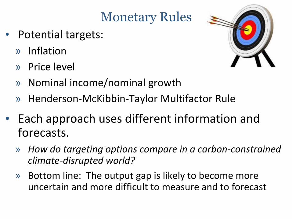
• Potential targets:

» Inflation

» Price level

» Nominal income/nominal growth

» Henderson-McKibbin-Taylor Multifactor Rule

• Each approach uses different information and forecasts.

» How do targeting options compare in a carbon-constrained climate-disrupted world?

» Bottom line: The output gap is likely to become more uncertain and more difficult to measure and to forecast

Inflation targeting

• The interest rate 𝑖𝑡» from the previous period 𝑖𝑡−1

• Actual inflation 𝜋𝑡

• Bank’s target inflation rate ത𝜋

• Feedback term 𝛼

» 𝑖𝑡 = 𝑖𝑡−1 + 𝛼 (𝜋𝑡 − ത𝜋 )

• Flexible inflation targeting (FIT) allows discretion in light of other goals.

• In practice, banks use inflation forecast: 𝜋𝑡,𝑡+1» forecast at time t of the inflation rate at time t+1

• 𝑖𝑡 = 𝑖𝑡−1 + 𝛼 (𝜋𝑡,𝑡+1 − ത𝜋 )

• A good forecast of inflation is important in inflation targeting regimes.

Contribution of Main Aggregates to Inflation in the United Kingdom (in percentage points) 2010-2018

Energy

http://www.myinflationtool.com/components-of-inflation/contributors-4-main-aggregates/

Measuring the Output Gap

• Forecast for inflation is an increasing function of the output gap.

• 𝜋𝑡,𝑡+1 = ത𝜋𝑡 + 𝑓(𝑌𝑡 − ത𝑌𝑡)

• 𝑌𝑡 = Output of the economy,

• ത𝑌𝑡 = Central bank’s assessment of the economy’s maximum potential output

• Both 𝑌𝑡 and ത𝑌𝑡 are uncertain estimates; central bankmay get the output gap wrong and thus use a poorforecast of inflation in its targeting strategy.

Price Level Targeting (PLT)

• 𝑃𝑡 = Actual price level

• ത𝑃𝑡 = Bank’s target price level

• Feedback term 𝛼

» 𝑖𝑡 = 𝑖𝑡−1 + 𝛼 (𝑃𝑡 − ത𝑃𝑡)

• In practice, price level targeting use a target that includes a trend.

» Strong historical dependence

» With a supply shock, the bank would not only offset the inflation shock but also tighten monetary policy even further to get price level back to the original trajectory

Nominal Income and Nominal GDP Growth Targeting (NIT)

• Avoid (nominal) recessions to maintain economic activity or rate of growth

» Balances reaction to inflation and output from supply shock

» Inflation rises x%, output falls x% => nominal income unchanged

• 𝑃𝑌𝑡 = Nominal income (Note: P is GDP deflator)

• 𝑃𝑌𝑡 = Bank’s target nominal income

» 𝑖𝑡 = 𝑖𝑡−1 + 𝛼 𝑃𝑌𝑡 − 𝑃𝑌t

• 𝑔𝑡 = Growth rate of nominal income (not level)

• ҧ𝑔𝑡 = Bank’s target growth rate

» 𝑖𝑡 = 𝑖𝑡−1 + 𝛼 (𝑔𝑡 − ҧ𝑔𝑡)

Henderson-McKibbin-Taylor (HMT) Rules

• Multiple feedback terms

» 𝑖𝑡 = 𝑖𝑡−1 + 𝛼 𝜋𝑡 − ത𝜋𝑡 + 𝛽 𝑌𝑡 − ത𝑌𝑡 + 𝛾 𝑃𝑌𝑡 − 𝑃𝑌𝑡

+ 𝛿 𝑒𝑡 − ҧ𝑒𝑡 + 𝜎(𝑀𝑡 − ഥ𝑀𝑡)

• Exchange rate (𝑒𝑡 with target ҧ𝑒𝑡)

• Money supply (𝑀𝑡 with target ഥ𝑀𝑡)

• Nominal GDP (𝑃𝑌𝑡 with target 𝑃𝑌𝑡 )

• Different weights in different countries

• Still have the challenge of estimating the output gap for some targets

• In the following discussion assume 𝜸= 𝜹= 𝝈 = 0

Monetary Rules

• Targeting rules: simple feedback from publicly observed economic conditions to interest rates

• Most monetary rules handle demand shocks well

• Managing supply shocks involves more tradeoffs across inflation and output stability goals.

• Climate change implies a world of greater supply and demand shocks.

Importance of the Output Gap

• Forecast for inflation is a function of the output gap.

• Output gaps estimation is important for each rule except nominal income growth targeting.

• If potential ex-post output growth is 1% lower then inflation will be 1% higher in a nominal income rule if the nominal growth target is achieved.

• Output gap estimation likely to deteriorate under climate change and climate policy during a transition

Key Issues for inflation

• All efficient climate regimes that price carbon have a rising carbon price to drive emissions lower over time

» Underlying inflation will have a new trend

• Carbon price volatility is higher under a cap and trade policy than under carbon tax of hybrid regime.

Monetary Rules & Climatic Disruption

• Monetary policymakers will face more frequent, larger, negative supply shocks

• Inflation targeting would tighten monetary policy to stem the rise in inflation; FIT might account for transitory nature but task is made difficult by imperfect real-time measurement of the output gap

» Fed’s estimates of the output gap under normal economic conditions have been prone to large errors

• PLT would react even more strongly, raising interest rates enough to reduce the price level back down to its target.

• In SIT, FIT, and PLT, the central bank would worsen the impact of the shock on economic activity.

Monetary Rules & Climatic Disruption

• HMT rule balanced reaction to output and inflation effects

• HMT rule involves difficulty of forecasting potential output and therefore the output gap.

• NIT relies only on nominal income.

» If potential output growth 1% lower than expected then inflation will be 1% higher than expected

» The central bank still limits the rise in expectations of higher inflation (within the band of error of output growth forecast) , preventing a wage-price spiral.

» Simple adherence to the policy rule gives a reasonable policy response.

• A critical issue for anchoring inflationary expectations is which target is more reliably forecasted?

Jointly Optimizing Climate and Monetary Policy

• Carbon tax

» Complex aggregate supply shock

» Tax increases costs of fossil inputs; lowers output

» Revenue use may be pro-growth (e.g. lowering other taxes)

» Net effect likely negative, but (we hope) small

• Example

» 3% target inflation rate, achieved each year historically

» Impose carbon tax at t=0, unanticipated, one-time increase

» Inflation rises, output falls

Price Level and Inflation Rate Impacts of a Simple Carbon Tax

.91

1.1

1.2

No

min

al P

rice

-3 -2 -1 0 1 2Year

Baseline Carbon Tax

Panel A: Price Level

05

1015

Infl

atio

n R

ate

-3 -2 -1 0 1 2

Panel B: Inflation Rate

Baseline Carbon Tax

Inflation returns to baseline in t=1

Note: Figure shows a 10% increase in the price level at the onset of the tax. Likely carbon taxes would have a smaller impact.

Central Bank Response Depends on Rule

• Strict inflation target

» Raise interest rates

» Slow growth

» Appreciate exchange rate, depress exports

» Reduce inflation, but worsen output decline

• Flexible inflation target

» Moderate interest rate increase

» But must detect carbon tax signal in noise of baseline

• Price level target

» Tighter policy to have deflation so price level returns to base

More Realistic Policy Scenario

• Carbon tax goes up each year in real terms

» Policy shock can change inflation, prices, and rate of growth of actual and potential output

» Example: carbon tax rises at 4 % real each year

.91

1.1

1.2

1.3

No

min

al P

rice

-3 -2 -1 0 1 2Year

Baseline Carbon Tax

Panel A: Price Level

05

1015

Infl

atio

n R

ate

-3 -2 -1 0 1 2

Panel B: Inflation Rate

Baseline Carbon Tax

Accommodating requires the

bank raise its target inflation rate

Other Climate Policies are Harder For Central Banks to Accommodate

• Emissions Trading

» Uncertain price signal owing to uncertain cost of abatement (stringency) & variation in economic growth

• Hybrid Policy

» Better than ETS

» Same predictability in short run as a carbon tax

• Regulatory/Subsidy/Standards Policy

» Most difficult for a given level of environmental performance

» Effects on output and prices would be opaque and hard to predict

Monetary Rules & Climatic Disruption

• Monetary policymakers will face more frequent, larger, negative supply shocks

• Inflation targeting would tighten monetary policy to stem the rise in inflation; FIT might account for transitory nature but task is made difficult by imperfect real-time measurement of the output gap

» Fed’s estimates of the output gap under normal economic conditions have been prone to large errors

• PLT would react even more strongly, raising interest rates enough to reduce the price level back down to its target.

• In SIT, FIT, and PLT, the central bank would worsen the impact of the shock on economic activity.

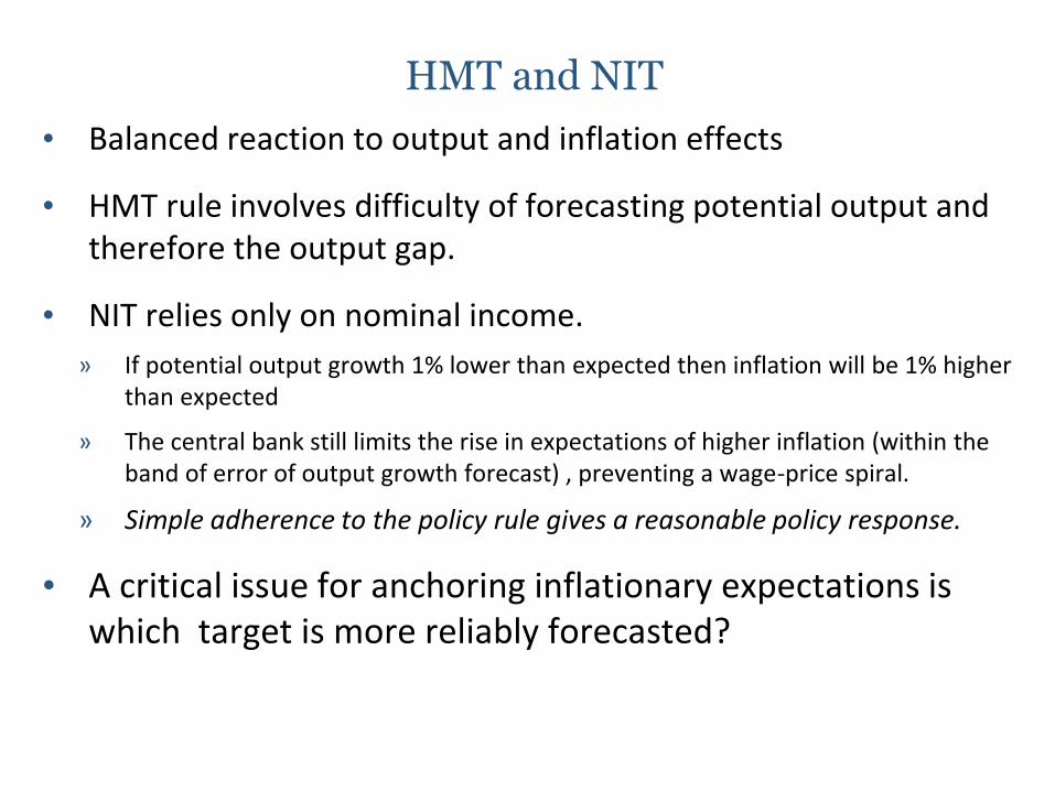
HMT and NIT

• Balanced reaction to output and inflation effects

• HMT rule involves difficulty of forecasting potential output and therefore the output gap.

• NIT relies only on nominal income.

» If potential output growth 1% lower than expected then inflation will be 1% higher than expected

» The central bank still limits the rise in expectations of higher inflation (within the band of error of output growth forecast) , preventing a wage-price spiral.

» Simple adherence to the policy rule gives a reasonable policy response.

• A critical issue for anchoring inflationary expectations is which target is more reliably forecasted?

Some Initial Evidence on relative forecast performance

• McKibbin W.J. and A. Panton (2018) “25 Years of Inflation Targeting in Australia: Are There Better Alternatives for the next 25 Years”, CAMA working paper . 19/2018.

Forecast errors of different targets

Source OECD and authors calculation

-2.50

-2.00

-1.50

-1.00

-0.50

-

0.50

1.00

1.50

2.00

1993 1994 1995 1996 1997 1998 1999 2000 2001 2002 2003 2004 2005 2006 2007 2008 2009 2010 2011 2012 2013 2014

OECD Forecast errors for Australia

Nominal GDP Real GDP Inflation

Some Further Model simulations with G-Cubed

0

5

10

15

20

25

30

35

40

45

0 1 2 3 4 5 6 7 8 9 10

US

Do

llars

-$

Years

Figure 2:Annual US carbon tax

-0.7

-0.6

-0.5

-0.4

-0.3

-0.2

-0.1

0

0 1 2 3 4 5 6 7 8 9 10

US

Years

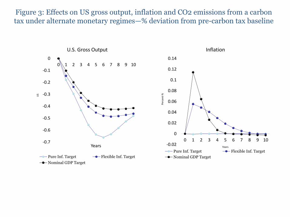
U.S. Gross Output

Pure Inf. Target Flexible Inf. Target

Nominal GDP Target

-0.02

0

0.02

0.04

0.06

0.08

0.1

0.12

0.14

0 1 2 3 4 5 6 7 8 9 10

Per

cen

t-%

Years

Inflation

Pure Inf. Target Flexible Inf. Target

Nominal GDP Target

Figure 3: Effects on US gross output, inflation and CO2 emissions from a carbon tax under alternate monetary regimes—% deviation from pre-carbon tax baseline

Figure 3: Effects on CO2 emissions from a carbon tax under alternate monetary regimes—% deviation from pre-carbon tax baseline

-25

-20

-15

-10

-5

0

0 1 2 3 4 5 6 7 8 9 10

% D

evia

tio

n

Years

CO2 Emissions

Pure Inf. Target Flexible Inf. Target Nominal GDP Target

Conclusion

• Central banks should expect more and larger supply shocks.

• Climate policy design that induces predictable and transparent price signals (like a carbon tax or a Hybrid) makes monetary policy response more transparent.

• Nominal Income Targeting appears to be better than inflation targeting because

» it avoids the need for a forecast of potential output

» does not require understanding precise nature of the climate-related shock

» It still anchors inflationary expectations to within a band

• A great deal more empirical research is needed

www.sensiblepolicy.com