Simple Energy Balance Climate Models:Literature Review and Analytic Techniques

Gerard Trimberger

due: March 10th, 2016

One of the simplest types of climate models are the energy balance models,

similar to the one created by M.I. Budyko in 1969 [2]. These types of models

attempt to predict the latitudinal temperature distribution, based on the idea

that the energy the Earth receives from the Suns radiation must balance the

radiation the earth is losing to space by reemission at its temperature T. They

also include a concept, known as the albedo effect, which takes into account

the reflection of the solar radiation off of the surface due to clouds, ice, snow,

etc. The ice-albedo feedback mechanism is of particular interest to climate

scientists because it serves to amplify any relatively small changes in solar ra-

diation. [13]

Problem Description

The issue of climate change is a widely debated topic that often arises in fields outside of the

scientific community. Most people accept the notion that the Earths climate is ever-changing,

and goes through very specific periods of transitory behavior. The most important question that

people usually ask is whether or not recent human activity has a direct impact on the trends that

we have observed. This question becomes significantly important when it comes to designing

1

conservation policies that require individuals, communities, businesses, governments, or nations

to follow a specific set of rules. If the policy makers are going to decide on a solution that is

best for all, as they should, although many dont, it is of utmost importance to understand the

complete picture of the arguments being presented. Obviously a large petroleum company does

not want to cut back its production, or be required to install specific regulatory inhibitors on the

basis of some article on science-fiction. While at the same time, we are all inhabitants of this

Pale Blue Dot, as Carl Sagan would call it, and therefore it is our moral responsibility to prevent

the destruction of our world by any man-made technology. Just as I think most would agree that

nuclear destruction of our planets ecosystem would be a moral failure, ignoring the blatant signs

of our own impacts on climate change would also qualify as a failure to act. Therefore, it is my

goal to review the current scientific literature on the topic of climate change and apply some of

the mathematic techniques that I have studied in this class, to create a simple mechanistic model

that provides some mathematical backing to the theory of climate change. By investigating

what has been done, concerning this particular problem, I hope to clarify some of the confusion

surrounding the climate change debacle and also provide myself with some of the knowledge

required to formulate my own mathematically sound argument regarding the issue.

I am going to focus my analysis on a specific type of climate model, often called simple

energy-balance climate models. As the name suggests, these models are rooted in Kirchhoff’s

Law of Thermal Radiation and Stefan-Boltzmann’s Law, relating temperature to black body

radiation . I will briefly discuss the empirical bases for any other proposed mechanisms that do

not follow directly from classical physics. [2]

My goal is to follow the trail of breadcrumbs back to the fundamental sources of informa-

tion. I have found various papers that link their models back to this Budyko paper, but I want to

keep following the trail back to the fundamental evidence being presented. Therefore the over-

all goal of this literature review/solution analysis, is not to present some novel climate change

2

model, but to instead give a complete introduction into the specifics of each of the papers in-

volved in creating these types of climate models, and also to introduce some simple techniques

on how to solve these system and produce scientifically relevant results.

The issue of climate change and how accurately it is modeled has extreme economic, politic,

social, and individual significancee. A study done by Cook et. al in 2013 suggested that approx-

imated 97% of scientists agree that climate change is real [4]. So my question then becomes

what are they all basing their data on? What if they are wrong, or missing some fundamental

assumption/simplification made at the very beginning that discards all further information.

[4]

As a good scientist, it is always good to go back to the beginning and build the model

from the ground up. Similarly, it is pretty obvious that environmental changes affect everyone!

Conclusions made from models can have huge impact on the conservation efforts required/ not

in order to preserve life, the way we know it, on this planet. We dont have anywhere else to

go at this time. The results of these climate models may Require companies and governments

world-wide to implement HUGE policy changes that in turn will cost copious amount of money,

time, and effort to fix. Is this all necessary? Or are we impeding future technological advances

by halting the current methods that we use for production of energy? Just as in conservation

biology, it is important to figure out who the big players are and how they affect the system.

If you focus your conservation efforts on the non-optimal step/stage, then you are inefficiently

utilizing your already limited resources. In this situation an accurate climate model could aid in

3

such decision-making processes.

If potentially every living in this planet is at danger of experiencing some of the most dra-

matic climate adjustments, isnt it our responsibility as the educated elite to ensure that everyone

in our country understands the consequences on our actions when they decide whether or not

to support the election of and decisions made by political figures? In order to reap the benefits

living in a democratic society, we must utilize our skills as mathematicians, engineers, and sci-

entists to objectively educate the masses on our logic-based predictions concerning the state of

our world, given the currently observed trends.

Background

[8]

4

Palioclimatology, or the study of ancient climates, provides us with a way to study the climate

change of the past. Bowen mentions several different classical climatic indicators that he places

into two exclusive categories: biological (fossils, coral reefs) and inorganic (evaporates, sed-

imentary deposits, morphological evidence). Specifically for this particular problem, we are

interested differentiating between hot and cold climates. He then explains how each method

has inherent flaws and introduces a more modern climatic indicator, utilizing the isotopes of

oxygen. Oxygen is made up of three stable isotopes, O16, O17, and O18. [1] Urey first presented

on this phenomenon in 1948 [14]. Later it was discovered that the relative abundance of oxygen

isotopes would depend in part on the temperature of the water during the time marine fossils

were depositing calcium carbonate, creating a water-carbonate equilibrium [15] [11] . This

created a geologic thermometer that could be used to predict the ancient climate of the earth.

From this information we can deduce that the earth goes through cycles of warming and cooling

and has been doing so for as long as we can record. This is a key factor to the climate model,

because it requires shows a correlation between temperature and atmospheric composition.

[2]

Humphreys presents a relationship be-

tween a change in atmospheric transparency,

due to recent volcanic activity, and the cor-

responding variation in direct radiation from

the sun [7]. Based on these observations, as

well as examining the data collected by the

Main Geophysical Observatory on monthly

temperature fluctuation between the years of

1881 and 1960, Budyko presented in his 1963

book, available only in Russian, an empirical

5

formula to categorize the outgoing radiation:

I = a+BT + (a1 +B1T )n

where, I - outgoing radiation, T is temperature at the earth’s surface, and n - ’cloudiness’ (in

fractions of a unit). This empircal formula was based on data from 260 stations around the

world. The value of the coefficients were postulated as a = 14.0;B = 0.14; a1 = 3.0;B1 =

0.10 [3]. This forms the first part of Budyko’s climate model.

[9]

The second portion of Budyko’s model is based on the heat balance of the earth-atmosphere

system presented by [9]. In this particular paper they explore the ’albedo’ effect, which in short

states that surfaces of the earth covered in snow/ice reflect more incoming solar radiation than

areas without such ground covering. This ’albedo’ parameter is denoted, α. For mean annual

conditions,

Q(1− α)− I = A

[12]

where A is loss/gain of heat as a result of atmo-

sphere/hydrosphere circulation, Q is solar radiation

coming to the outer boundary of the atmosphere, and

again α - captures ’albedo’ effect. Budyko 1969 and

North 1975 both modeled the absorption function, 1−α

(shown to the right), with the simplification of setting a2 = 0, thereby modeling ’ice-covered’

and ’ice-free’ regions [2] [12].

6

Simplifications

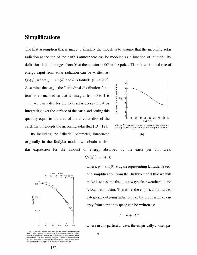
The first assumption that is made to simplify the model, is to assume that the incoming solar

radiation at the top of the earth’s atmosphere can be modeled as a function of latitude. By

definition, latitude ranges from 0o at the equator to 90o at the poles. Therefore, the total rate of

[6]

energy input from solar radiation can be written as,

Qs(y), where y = sin(θ) and θ is latitude (0 → 90o).

Assuming that s(y), the ’latitudinal distribution func-

tion’ is normalized so that its integral from 0 to 1 is

= 1, we can solve for the total solar energy input by

integrating over the surface of the earth and setting this

quantity equal to the area of the circular disk of the

earth that intercepts the incoming solar flux [13] [12].

By including the ’albedo’ parameter, introduced

originally in the Budyko model, we obtain a sim-

ilar expression for the amount of energy absorbed by the earth per unit area:

Qs(y)(1− α(y))

[12]

where, y = sin(θ), θ again representing latitude. A sec-

ond simplification from the Budyko model that we will

make is to assume that it is always clear weather, i.e. no

’cloudiness’ factor. Therefore, the empirical formula to

categorize outgoing radiation, i.e. the reemission of en-

ergy from earth into space can be written as:

I = a+BT

where in this particular case, the empirically chosen pa-

7

rameter values are a = 202 and B = 1.90, described

below [2]. It is important to note that the difference be-

tween solar reflection and outward radiation. Solar reflection does not change the wavelength

of the light because the light simply bounces off of the ’reflective’ surface. Conversely, earthly

[8]

emission involves a change in wavelength, from ultraviolet to infrared, which occurs because

earth’s surface molecules absorb the incoming light and re-emit it at a lower frequency (IR).

Again, using Stefan-Boltzmann’s Law we can assume

I(y) = σT 4

which states that the rate of total energy radiated per unit surface area is proportional to the

fourth power of the ’black body’s’ temperature. Due to the fact that the earth is not a black body,

8

the calculations become difficult, therefore we must simplify by taking a linear approximation

around 0o:

I(y) = a+B(T − T0)

where T0 = 0o C or 273o K.

[5]

Graves, Lee, and North applied such model to a 10-year data set of surface temperature

versus ’Outgoing Longwave Radiation’ (OLR). They used this linearizion to solve for particular

values for the coefficients above, a = 202 and B = 1.90 [5]. In order to simplify the ’albedo’

effect we will made the simplification similar to Budyko’s and set an albedo constant for ’ice-

9

covered’ and ’ice-free’ regions, setting the ’ice-line’ to the average between the two,

α(y) =

αcovered = 0.62 y > yice

αfree = 0.32 y < yice

αedge = (αcovered + αfree)/2 = 0.47 y = yice

where T (yice) = Tc = −10o C. This is based on the idea that −10o C is a good estimate for the

temperature at which glaciers can persist, slightly below freezing [2] [13].

[2]

Finally, we will discuss the sim-

plifications made on the transport

mechanism. In order to accurately

model circulation patterns present

in the earth’s atmosphere-ocean sys-

tem, a complex dynamical system

would need to be designed. More

modern models have taken this ap-

proach to improve their accuracy,

however that is beyond the scope of

my project. I wish to model transport using the simple model that Budyko proposed, by lumping

all of the process into a single ’relaxation’ term:

A = β(T − Tp)

where β is an empirical parameter, which measures the efficiency of the model in transporting

energy polewards, and Tp is the planetary mean temperature [2] [13]. Based on satellite mea-

surement of the solar constant, a commonly accepted value for β = 1.6B, where by was also

found empirically by Graves, Lee, and North [5].

10

Mathematical Model

Following all of the simplifications made in the previous steps, we can now construct our model

equation. Given the title of this particular class of climate models, i.e. ’Energy-balance,’ it is

importantly to explicitly state what this means. In words, the rate of the change of the earth’s

surface temperature should be equal to the net solar absorption minus outward radiation, plus

that from the transport mechanism:

R∂T

∂t= F (T )

F (T ) = Qs(y)(1− α(y))− I(y) +D(y)

Noting that, ∫ 1

0

s(y)dy = 1

α(y) =

αcovered = 0.62 y > yice

αfree = 0.32 y < yice

αedge = (αcovered + αfree)/2 = 0.47 y = yice

I(y) = a+B(T − T0)

D(y) = −β(T − Tp)

Therefore in order to solve this system analytically, we must break the piecewise functions

into the 3 corresponding states: ’ice-free globe,’ ’ice-covered globe,’ and ’partially ice-covered

globe.’ The relevant albedo ratios are given as α(y) (above) [2] [13]. Making one final sim-

plication, that the average weather patterns seen in Northern Hemisphere would replicate the

patterns observed in the Southern Hemisphere, we notice that the problem becomes symmet-

ric about the equator. Therefore, the global mean temperature of the planet, Tp, becomes the

average mean temperature of the hemisphere:

Tp =

∫ 1

0

T (y)dy

11

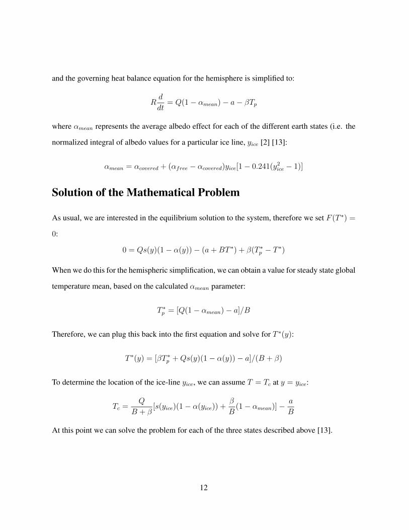
and the governing heat balance equation for the hemisphere is simplified to:

Rd

dt= Q(1− αmean)− a− βTp

where αmean represents the average albedo effect for each of the different earth states (i.e. the

normalized integral of albedo values for a particular ice line, yice [2] [13]:

αmean = αcovered + (αfree − αcovered)yice[1− 0.241(y2ice − 1)]

Solution of the Mathematical Problem

As usual, we are interested in the equilibrium solution to the system, therefore we set F (T ∗) =

0:

0 = Qs(y)(1− α(y))− (a+BT ∗) + β(T ∗p − T ∗)

When we do this for the hemispheric simplification, we can obtain a value for steady state global

temperature mean, based on the calculated αmean parameter:

T ∗p = [Q(1− αmean)− a]/B

Therefore, we can plug this back into the first equation and solve for T ∗(y):

T ∗(y) = [βT ∗p +Qs(y)(1− α(y))− a]/(B + β)

To determine the location of the ice-line yice, we can assume T = Tc at y = yice:

Tc =Q

B + β[s(yice)(1− α(yice)) +

β

B(1− αmean)]−

a

B

At this point we can solve the problem for each of the three states described above [13].

12

Results/Discussion

For the ’ice-free globe,’ we set α(y) = α1 = 0.32 for all y. By including the parameter values

previously discussed and by utilizing the definition of ’ice-free’ as T ∗(ypoles = 1) > Tc, we can

calculate the predicted global average temperature:

T ∗p = [343(0.68)− 202]/1.9 = 16oC

Using a similar argument for the ’ice-covered globe,’ except setting α(y) = α2 = 0.62 for all y

and remembering ’ice-covered’ means that T ∗(yequator = 0) > Tc, we can calculate the global

average temperature for this scenario:

T ∗p = [343(0.38)− 202]/1.9 = −38oC

The solution to the problem with ’partially ice-covered globe’ is simply a combination of the

previous two solutions. Instead of assuming a constant α value for all y, we would assume the

’ice-covered,’ α2, for regions > yice and the ’ice-free,’ α1, for regions < yice. For the region

exactly at y = yice, we could assume α = (α1 + α2)/2 as shown above [2] [13].

The calculations for the stability of these regions goes beyond the scope of this project but

is mentioned in Cahalan and North (1979), as well as Budyko (1972). I did not investigate these

particular arguments for my literature review.

Improvement

This leads well into future improvements for this project. I would definitely want to do a lit-

erature review of the above mentioned scientific articles to better understand the processes by

which these groups ’solved’ the temperature equilibrium stability. My main focus was to work

backwards to formulate the argument from ground up as to why the Budyko 1969 model con-

sistently appears as a reference for most of the more ’modern’ energy-balance climate models.

13

Now the task would be to work the other way. To determine how the Budyko 1969 model can

be expanded on or modified in order to produce more accurate results.

One common critique that I noticed regarding this particular model was the type of transport

mechanism utilized. Budyko 1969, as well as the simplification presented by Tung, models

the temperature transport system (i.e. the atmosphere and hydrosphere systems) as a simple

’relaxation’ term [2] [13]:

D(y) = β(Tp − T )

This was part of the reason that this particular model was chosen by Tung as a prime teaching

tool. At the same time the error in the simplification can create significant issues when relating

the model predictions to disaster-prevention policies. Therefore, another possible direction for

improvement would be to do literature search/review for different temperature transport mech-

anisms.

[10]

14

When investigating the most recent climate models, it becomes very clear that this is an

extremely interdisciplinary field of study. The table above shows just some of the systems

that the more recent models attempt to include. Each of these individual mechanistic-based

models are often the work interdisciplinary groups themselves. When it is coupled all together

it combines some of the top names in science, with the most complex computer simulation

techniques to provide some insight into the possible effects of our behavior on global climate

change, and this is just the mechanism of climate change! Most models do not even begin to

correlate the effects of human behavior with the corresponding influence it is having on the

problem. In this way the problem becomes more complex every day and it is up to panels, such

as IPCC, to sift through the data and observations to come up with an accurate climate change

model that most can agree on.

Conclusions

Overall, this was a very exciting project. I was able to work backwards, constantly asking the

question ”Why?, to uncover some of the fundamental assumptions (empirical or more mecha-

nistic) that are required to design simple energy-balance climate models. I focused the majority

of my research on the Budyko 1969 climate model because I felt that it has withstood the test of

time, in the sense that it is still being discussed today, despite it very obviously lack of complex-

ity. I think that this shows that it is still work investigating, because many of the fundamental

assumptions made in more modern models follows a similar train of thought. Obviously, the

equations derived and the systems generated are more complex, but more often than not they are

derived with similar processes in mind. I hope to apply the information that I have learned re-

garding techniques used in both model design, as well as solution generation, to future problems

with similar design constraints. Although I was not able to answer the big question of whether

or not global warming is scientifically relevant, I was able to broaden my overall understanding.

15

References

[1] Robert Brown. Paleotemperature Analysis: Methods in Geochemistry and Geophysics.

1966.

[2] M. I. Budyko. The effect of solar radiation variations on the climate of the earth. Tellus,

21(5):611–619, 1969.

[3] MI Budyko et al. Atlas of the heat balance of the earth. Academy of Sciences, Moscow,

69, 1963.

[4] John Cook, Dana Nuccitelli, Sarah A Green, Mark Richardson, Brbel Winkler, Rob Paint-

ing, Robert Way, Peter Jacobs, and Andrew Skuce. Quantifying the consensus on an-

thropogenic global warming in the scientific literature. Environmental Research Letters,

8(2):024024, 2013.

[5] Charles E Graves, Wan-Ho Lee, and Gerald R North. New parameterizations and sensi-

tivities for simple climate models. Journal of geophysical research, 98(D3):5025–5036,

1993.

[6] Isaac M. Held and Max J. Suarez. Simple albedo feedback models of the icecaps. Tellus,

26(6):613–629, 1974.

[7] William Jackson Humphreys. Physics of the Airs, 2nd Ed. Franklin Institute of the state

of Pennsylvania, 1929.

[8] Richard S. Lindzen. Some coolness concerning global warming. Bull. Amer. Meteor. Soc.,

71(3):288 – 299, 1990.

[9] Syukuro Manabe and Richard T Wetherald. Thermal equilibrium of the atmosphere with

a given distribution of relative humidity. 1967.

16

[10] many contributors. Climate Change 2013: The Physical Science Basis. Intergovernmental

Panel on Climate Change, 2013.

[11] W.G. Mook. Paleotemperatures and chlorinities from stable carbon and oxygen isotopes

in shell carbonate. Palaeogeography, Palaeoclimatology, Palaeoecology, 9(4):245 – 263,

1971.

[12] Gerald R. North. Theory of energy-balance climate models. J. Atmos. Sci., 32(11):2033 –

2043, 1975.

[13] K. K. Tung. Topics in Mathematical Modeling. Princeton University Press, 2007.

[14] Harold C. Urey. Oxygen isotopes in nature and in the laboratory. Science, 108(2810):489–

496, 1948.

[15] Harold Clayton Urey, Heinz A Lowenstam, Samuel Epstein, and Charles R McKinney.

Measurement of paleotemperatures and temperatures of the upper cretaceous of england,

denmark, and the southeastern united states. Geological Society of America Bulletin,

62(4):399–416, 1951.

17