climate phenomena and their relevance for future regional ... · 14sm-3 climate phenomena and their...
TRANSCRIPT
14SM-1
14SM
This chapter supplementary material should be cited as:Christensen, J.H., K. Krishna Kumar, E. Aldrian, S.-I. An, I.F.A. Cavalcanti, M. de Castro, W. Dong, P. Goswami, A. Hall, J.K. Kanyanga, A. Kitoh, J. Kossin, N.-C. Lau, J. Renwick, D.B. Stephenson, S.-P. Xie and T. Zhou, 2013: Cli-mate Phenomena and their Relevance for Future Regional Climate Change Supplementary Material. In: Climate Change 2013: The Physical Science Basis. Contribution of Working Group I to the Fifth Assessment Report of the Intergovernmental Panel on Climate Change [Stocker, T.F., D. Qin, G.-K. Plattner, M. Tignor, S.K. Allen, J. Boschung, A. Nauels, Y. Xia, V. Bex and P.M. Midgley (eds.)]. Available from www.climatechange2013.org and www.ipcc.ch.
Coordinating Lead Authors:Jens Hesselbjerg Christensen (Denmark), Krishna Kumar Kanikicharla (India)
Lead Authors:Edvin Aldrian (Indonesia), Soon-Il An (Republic of Korea), Iracema Fonseca Albuquerque Cavalcanti (Brazil), Manuel de Castro (Spain), Wenjie Dong (China), Prashant Goswami (India), Alex Hall (USA), Joseph Katongo Kanyanga (Zambia), Akio Kitoh (Japan), James Kossin (USA), Ngar-Cheung Lau (USA), James Renwick (New Zealand), David B. Stephenson (UK), Shang-Ping Xie (USA), Tianjun Zhou (China)
Contributing Authors:Libu Abraham (Qatar), Tércio Ambrizzi (Brazil), Bruce Anderson (USA), Osamu Arakawa (Japan), Raymond Arritt (USA), Mark Baldwin (UK), Mathew Barlow (USA), David Barriopedro (Spain), Michela Biasutti (USA), Sébastien Biner (Canada), David Bromwich (USA), Josephine Brown (Australia), Wenju Cai (Australia), Leila V. Carvalho (USA/Brazil), Ping Chang (USA), Xiaolong Chen (China), Jung Choi (Republic of Korea), Ole Bøssing Christensen (Denmark), Clara Deser (USA), Kerry Emanuel (USA), Hirokazu Endo (Japan), David B. Enfield (USA), Amato Evan (USA), Alessandra Giannini (USA), Nathan Gillett (Canada), Annamalai Hariharasubramanian (USA), Ping Huang (China), Julie Jones (UK), Ashok Karumuri (India), Jack Katzfey (Australia), Erik Kjellström (Sweden), Jeff Knight (UK), Thomas Knutson (USA), Ashwini Kulkarni (India), Koteswara Rao Kundeti (India), William K. Lau (USA), Geert Lenderink (Netherlands), Chris Lennard (South Africa), Lai-yung Ruby Leung (USA), Renping Lin (China), Teresa Losada (Spain), Neil C. Mackellar (South Africa), Victor Magaña (Mexico), Gareth Marshall (UK), Linda Mearns (USA), Gerald Meehl (USA), Claudio Menéndez (Argentina), Hiroyuki Murakami (USA/Japan), Mary Jo Nath (USA), J. David Neelin (USA), Geert Jan van Oldenborgh (Netherlands), Martin Olesen (Denmark), Jan Polcher (France), Yun Qian (USA), Suchanda Ray (India), Katharine Davis Reich (USA), Belén Rodriguez de Fonseca (Spain), Paolo Ruti (Italy), James Screen (UK), Jan Sedláček (Switzerland) Silvina Solman (Argentina), Martin Stendel (Denmark), Samantha Stevenson (USA), Izuru Takayabu (Japan), John Turner (UK), Caroline Ummenhofer (USA), Kevin Walsh (Australia), Bin Wang (USA), Chunzai Wang (USA), Ian Watterson (Australia), Matthew Widlansky (USA), Andrew Wittenberg (USA), Tim Woollings (UK), Sang-Wook Yeh (Republic of Korea), Chidong Zhang (USA), Lixia Zhang (China), Xiaotong Zheng (China), Liwei Zou (China)
Review Editors:John Fyfe (Canada), Won-Tae Kwon (Republic of Korea), Kevin Trenberth (USA), David Wratt (New Zealand)
Climate Phenomena andtheir Relevance for FutureRegional Climate ChangeSupplementary Material

14SM-2
14SM
Table of Contents
14.SM.1 Monsoon Systems ......................................... 14SM-3
14.SM.2 El Niño-Southern Oscillation and Its Flavours ..................................................... 14SM-6
14.SM.3 Annular and Dipolar Modes ...................... 14SM-6
14.SM.4 Large-scale Storm Systems ........................ 14SM-7
14.SM.5 Additional Phenomena of Relevance ................................................. 14SM-10
14.SM.6 Future Regional Climate Change ........... 14SM-10
References .......................................................................... 14SM-56

14SM-3
Climate Phenomena and their Relevance for Future Regional Climate Change Chapter 14 Supplementary Material
14SM
14.SM.1 Monsoon Systems
14.SM.1.1 Global Overview
Monsoons are seasonal phenomena and are responsible for the major-ity of summer rainfall within the tropics. In the classical view, the mon-soon is driven by the seasonal cycle of solar heating and difference in thermal inertia of land and ocean that establish a land–sea tempera-ture difference. This contrast, with the land being warmer than the sur-rounding ocean in late spring and summer, gives favourable conditions for the occurrence of convection in the summer hemisphere, allowing the monsoon to be viewed as a seasonal migration of the Inter-Tropi-cal Convergence Zone (ITCZ). As the monsoon season matures, latent heat released by convection high above the land surface helps to pull in additional moisture from nearby oceans over the land, maintaining the wet season. This thermal forcing depends on large-scale orography and controls the regional monsoon domain and intensity. The land–sea temperature difference is projected to become larger in the summer season as seen from larger warming over land than ocean (Section 12.4.3.1 and Annex I Figures AI.4 to AI.5). However, this does not lead to a generally stronger monsoon circulations in the future, as chang-es in regional monsoon characteristics are rather complex. In broad terms, the precipitation characteristics over Asia-Australia, Americas and Africa can be viewed as an integrated global monsoon system, associated with a global-scale persistent atmospheric overturning cir-culation (Trenberth et al., 2000). Wang and Ding (2008) demonstrated that the global monsoon is the dominant mode of annual variation of the tropical circulation, characterizing the seasonality of the Earth’s climate in tropical latitudes. The monsoon-affected region is, however, not uniform in the historical record (Conroy and Overpeck, 2011), and it could vary in the future.
14.SM.1.2 Definition of Global Monsoon Area, Global Monsoon Total Precipitation and Global Monsoon Precipitation Intensity
The global monsoon area (GMA) is defined as where the annual range of precipitation exceeds 2.5 mm day–1. Here, the annual range is defined as the difference between the May to September (MJJAS) mean and the November to March (NDJFM) mean. The global monsoon total precipitation (GMP) is defined as the mean of summer rainfall in the monsoon area. The global monsoon precipitation intensity (GMI) is defined as GMP divided by GMA.
14.SM.1.3 Definition of Monsoon Onset, Retreat and Duration
Monsoon onset date, retreat date and its duration are determined using the criteria proposed by Wang and LinHo (2002) utilizing only precipita-tion data. Based on the regionally averaged relative climatological mean daily precipitation, which is the difference between the climatological daily precipitation and dry month (January in the Northern Hemisphere and July in the Southern Hemisphere ) mean precipitation, the onset (retreat) date is defined as the date when the relative precipitation first exceeds (last drops below) 5 mm day–1, and the duration is defined as their difference. The daily climatology of precipitation was defined as the sum of the first 12 harmonics of daily average precipitation.
14.SM.1.3.1 South America Monsoon System
Although the changes in wind direction from winter to summer occur only in a small area within South America, there are large differences in the atmospheric circulation and in sources of humidity from winter to summer. These differences are related to the rainy season in central and southeastern Brazil, which begins at the middle/end of spring and finishes at the middle/end of autumn (Silva and Carvalho, 2007; Raia and Cavalcanti, 2008).
The lifecycle of the South America Monsoon System (SAMS) is dis-cussed in Raia and Cavalcanti (2008), where the main atmospheric characteristics in the onset and demise are related to the rainy season. The changes in humidity flux linked to the low-level flow changes over the northernmost part of South America and the Amazonia region, eastward shifting of subtropical high, strong northwesterly moisture flux east of tropical Andes, are the main features in the onset. At high levels, the Bolivian High and the Northeast High Level Cyclonic Vortex are established during this period. The moisture flux from the Atlantic Ocean over northern South America, crossing the Amazonia region and directed to the southeast, increases the humidity over southeastern Brazil, favouring the intensification of convection there. The resulting coupling between Amazonia convection and frontal systems, and the favourable high-level anomalous circulation over the continent, often associated with the Pacific–South American (PSA) wave train, origi-nate the South Atlantic Convergence Zone (SACZ). The whole cycle of SAMS comprises three stages, the rainfall beginning over northwestern South America, SACZ establishment and precipitation increase over the mouth of Amazon River (Nieto-Ferreira and Rickenbach, 2010).
In a recent review of SAMS, the main structure and lifecycle; the onset features; and the diurnal, mesoscale, synoptic, intraseasonal, interan-nual and inter-decadal variability are discussed, as well as the long-term variability and climate change (Marengo et al., 2010).
Jones and Carvalho (2013) used the Large–scale Index for South Ameri-ca Monsoon LISAM index (Silva and Carvalho, 2007), which is obtained from the combined Empirical Orthogonal Function (EOF) analysis of low-level (850 hPa) zonal and meridional winds, temperature and spe-cific humidity.
Seasonal precipitation variability over South America is well represent-ed by Atmospheric General Circulation Models (AGCMs) and Coupled General Circulation Models (CGCMs), mainly the large differences between summer and winter. However, the intensity or configuration of rainfall patterns in the summer season is not well represented by some models. Vera et al. (2006), and Vera and Silvestri (2009) analysed seven models of World Climate Research Programme–Coupled Model Intercomparison Project Phase 3 (WCRP–CMIP3) for the 20th century and showed that seasonal precipitation differences are well represent-ed. Some models capture the precipitation variability, indicated by the standard deviation, and maximum rainfall associated with the SACZ, in the first three months (January, February and March (JFM)) and the last three months (October, November and December (OND)), but with different intensities compared to the observations. The ensemble mean precipitation analysis of nine models WRCP-CMIP3, also for the 20th century, by Seth et al. (2010), indicated reasonable comparisons of

14SM-4
Chapter 14 Supplementary Material Climate Phenomena and their Relevance for Future Regional Climate Change
14SM
SON and DJF with observations, although specific features as the ITCZ intensity and position, and extension of SACZ to the ocean, were not properly represented.
Other comparisons of IPCC CMIP3 models with observed precipitation, in Bombardi and Carvalho (2009), show that some models capture the main features of SAMS, as the NW–SE band from Amazonia to the southeast, representing SACZ occurrences, and the Atlantic ITCZ. How-ever, intensities and positions of maximum precipitation are not well represented. The annual cycle in small areas of South America is not well represented by the majority of models, but has good representa-tion in southern Amazon and central Brazil. The duration of the rainy season is overestimated over west South America and underestimated over central Brazil, in CMIP3 models (Bombardi and Carvalho, 2009). Some aspects of the humidity flux over South America are well repre-sented by a set of CMIP3 models (Gulizia et al., 2013).
The South Indian, Pacific and Atlantic Oceans have a role on SAMS variability (Drumond and Ambrizzi, 2005; Grimm et al., 2007); therefore it is expected that projected changes in sea surface temperature (SST) patterns may affect this variability.
Changes in the annual cycle of the SAMS, from the 20th to the end of 21st century, projected by nine models, considering the A2 scenario were presented by Seth et al. (2010). The ensemble shows increased precipitation over SESA region (southern sector of southeastern South America).
Some CMIP3 models project precipitation increase in austral summer and a decrease in austral spring in the SAMS region (Seth et al., 2011). Precipitation increase at the end of the monsoon cycle and reduced precipitation in the onset in central monsoon region could indicate a shifting in the lifecycle monsoon period. These changes were related to less moisture convergence in the austral spring and more convergence during summer. During the dry season, the changes are very small. The warmer troposphere and increased stability due to global warming (Chou and Chen, 2010) act as a remote mechanism to reduced precip-itation of SAMS in the winter. During summer, the local mechanisms, such as increased evaporation and decreased stability, contribute to the increased precipitation. Both mechanisms seem to reduce precip-itation during spring, when there is not enough soil moisture and still atmospheric stability.
Idealized experiments with a coupled atmospheric–ocean model sub-jected to increasing carbon dioxide (CO2) show intensification of the precipitation difference between summer and winter in the global monsoon regions, including the SAMS region (Cherchi et al., 2011).
14.SM.1.4 What Is a Stronger East Asian Summer Monsoon?
Unlike the Indian summer monsoon, which can be defined in terms of simple scalar indices partly due to its homogeneity in rainfall dis-tribution, it is more complicated to define an index for the East Asian Summer Monsoon (EASM; Zhou et al., 2009b). Wang et al. (2008) dis-cussed the meanings of 25 existing EASM indices and classify these indices into five categories: the east–west thermal contrast, north–
south thermal contrast, the shear vorticity of zonal winds, the south-westerly monsoon and the South China Sea monsoon. Although the existing indices highlight different aspects of the EASM, they agree well in the traditional Chinese meaning of a strong EASM, viz. an abnormal northward extension of the southerlies into North China. The associated precipitation anomaly appears as excessive rainfall in North China along with a deficient Meiyu in the Yangtze River Valley (see Figure 3 of Zhou et al., 2009b for patterns of precipitation over eastern China associated with stronger and weaker monsoon circulations).
14.SM.1.5 Present Understanding of the Weakening Tendency of East Asian Summer Monsoon Circulation Since the End of the 1970s
From 1950 to present, the EASM circulation has experienced an inter-decadal scale weakening after the 1970s (Figure 14.SM.1), result-ing in deficient rainfall in North China but excessive rainfall in central East China along 30°N (Hu, 1997; Wang, 2001; Gong and Ho, 2002; Yu et al., 2004). The weakening of EASM is associated with weakening of 850 hPa southwesterly wind (Xu et al., 2006), a tropospheric cooling over East Asia (Yu and Zhou, 2007; Zhou and Zhang, 2009), a westward extension of the western Pacific Subtropical High (Zhou et al., 2009a), a zonal expansion of South Asian High (Gong and Ho, 2002; Zhou et al., 2009a) and an enhanced subtropical westerly jet (Zhang et al., 2006; Yu and Zhou, 2007). The circulation changes have led to significant changes in mean and extreme precipitation (Zhai et al., 2005), frequen-cy and intensity of rainfall events (Qian et al., 2009; Yu et al., 2010c; Bennartz et al., 2011; Li et al., 2011a; Liu et al., 2011; Guo et al., 2013).
The weakening of the EASM circulation since the 1970s is dominat-ed by natural decadal variability (Lei et al., 2011; Zhu et al., 2012). The combination of tropical ocean warming associated with the phase transition of Pacific Decadal Oscillation (PDO; see Figure 14.SM.1 for the EASM circulation response to PDO-related SST forcing in AGCM experiments, Zhou et al., 2008; Li et al., 2010c; Zhou and Zou, 2010) and weakening of atmospheric heating over the Tibetan Plateau leads to a reduction of land–sea thermal contrast, and thereby a weakened monsoon circulation (Ding et al., 2008, 2009; Duan and Wu, 2008). The weakening of the Tibetan Plateau heating is caused by increased snow cover and depth in winter associated with North Atlantic Oscilla-tion (NAO) phase change and North Indian Ocean warming (Zhang et al., 2004; Ding and Wang, 2009). The specified aerosol forcing cannot reproduce the observed EASM circulation changes (Figure 14.SM.1).
14.SM.1.6 Details of Precipitation Changes over East China Associated with the Weakening Tendency of East Asian Summer monsoon Circulation Since the End of the 1970s
Precipitation changes due to the weakening tendency of the EASM circulation are evident in both mean and extreme precipitation (Zhai et al., 2005). Analysis based on daily data shows that both the frequency and amount of light rain have decreased in eastern China during 1956–2005, with high spatial coherency, attributable in part to the warm rain suppression by aerosols (Qian et al., 2009; Liu et al., 2011; McKee et al., 2011). The results of early studies based on daily precipitation data have been argued by recent studies based on hourly data. Recent

14SM-5
Climate Phenomena and their Relevance for Future Regional Climate Change Chapter 14 Supplementary Material
14SM
analysis of hourly data finds that the rainfall amount and frequency have significantly increased (decreased) but the rainfall intensity has decreased (increased) in the middle to lower reaches of the Yangtze River valley (North China).The “wetter South-drier North” pattern of mean precipitation is mostly attributed to moderate and low inten-sity rainfall (≤10 mm hr–1) rather than the extreme rainfall (≥20 mm/hour, Yu et al., 2010c), although the frequency of extreme rain events has substantially increased along the Yangtze River (Qian et al., 2007a, 2007b). The drier North China is dominated by decreased long duration (persist longer than 6 hours) rainfall events, especially those occurring between midnight and morning, while the wetter South China is asso-ciated with both the substantially increased frequency and amount of long duration precipitation (Li et al., 2011a).
Figure 14.SM.1 | Time series of East Asian Summer Monsoon (EASM) indices (bars) and their trend lines (dashed line) from National Centers for Environmental Predic-tion/National Center for Atmospheric Research (NCEP/NCAR) reanalysis, (b) European Centre for Medium range Weather Forecast (ECMWF) 40-year reanalysis of the global atmosphere and surface conditions (ERA-40 reanalysis, (c) Global Ocean Global Atmo-sphere (GOGA) run of Community Atmosphere Model version 3 (CAM3), (d) difference between GOGAI and GOGA run of CAM3. Also shown is the slope of the trend (b, change per 50 years). The EASM index is defined as the normalized zonal wind shear between 850 and 200 hPa averaged over 20°N to 40°N and 110°E to 140°E. GOGA run is forced by observed monthly SSTs over the global oceans from 1950 to 2000, while GOGAI is driven by global sea surface temperature (SST) plus IPCC 20th century atmospheric (primarily greenhouse gases and direct aerosol) forcings (Li et al., 2010b). This figure demonstrated that the weakening tendency of EASM circulation was driven by Pacific Decadal Oscillation (PDO).
14.SM.1.7 Uncertainties in the Aerosol Effects on the Observed East Asian Summer Monsoon Changes
The aerosol effect on EASM circulation and precipitation changes during the past 60 years has large uncertainties. The combined effect of BC and sulphate aerosols is hypothesized to produce a weakened EASM but enhanced precipitation over South China (Liu et al., 2009a). Sulphate aerosol may reduce the surface heating over land and dimin-ish land–sea thermal contrast ). The increases of both sulphate and black carbon aerosol since 1950 may have weakened the land-sea temperature contrast and curtailed the monsoon in East Asia by acting to reduce September’s rainfall (Guo et al., 2013). However, some aer-osols (e.g., sulphate) could cool the atmosphere and surface but some (e.g., EC and dust) could cool the surface and warm the atmosphere. So the aerosol forcing impacts on land-ocean temperature contrast and hence EASM circulation is not well known yet. GCM experiments have shown that increased aerosol optical depth in China causes a notice-able increase in precipitation in the southern part of China in July, through induced surface cooling in mid-latitude leading to strengthen-ing of the Hadley circulation (Gu et al., 2006). However, the inclusion of black carbon in the simulations does not necessarily produce the observed “north drought/south flood” precipitation pattern in China during the past 50 years (Wang and Zhou, 2005).Sulphate aerosols have been shown to affect rainfall redistribution over East Asia in late spring and early summer, and weaken monsoon rainfall through direct (Kim et al., 2007; Liu et al., 2009b) or semi-direct (Zhang et al., 2009) effects. However, these results do not explain the observations of the north/dry and south/wet pattern in East Asia in recent decades. Some GCM experiments showed that the aerosol forcing may not be a forc-ing mechanism for the weakening tendency of EASM circulation and precipitation (Li et al., 2007, 2010c).
14.SM.1.8 The Dynamics of the North American Monsoon System
Seasonal mean precipitation in the North American monsoon region (mainly Mexico and the extreme Southwestern USA) is generally con-trolled by the establishment of a continental-scale upper-level anticy-clone and a lower-level thermal low (Higgins et al., 1997; Vera et al., 2006), it is also under the influence of factors operating at multiple spatial and temporal scales, including propagating waves and troughs in the tropics, synoptic disturbances and fronts entering the domain from the mid-latitudes and land-falling tropical cyclones (Douglas and Englehart, 2007). It is fed by two distinct, relatively narrow low-level moisture sources—the Great Plains Low-level Jet (LLJ) to the east of the Sierra Madres, which is approximately 200 to 400 km in width, and the narrower Gulf of California LLJ to the west of the Sierra Madres, which is approximately 100 km in width. Further, the large-scale cir-culation features—including the upper-tropospheric monsoon ridge, the North Atlantic subtropical (or Bermuda) high, the ITCZ, and the subtropical jet stream—in which these phenomena develop are mod-ified by slowly evolving coupled climate features associated with the PDO, the Atlantic Multi-decadal Oscillation (AMO) and solar activity (van Loon et al., 2004; Feng and Hu, 2008; Seager et al., 2009; Metcalfe et al., 2010; Arias et al., 2012). Dust aerosol may also have an impact on the North American monsoonal precipitation (Zhao et al., 2012).

14SM-6
Chapter 14 Supplementary Material Climate Phenomena and their Relevance for Future Regional Climate Change
14SM
14.SM.2 El Niño-Southern Oscillation and Its Flavours
The El Niño-Southern Oscillation (ENSO) is a coupled ocean–atmos-phere phenomenon naturally occurring at the interannual time scale. El Niño involves anomalous warming of tropical eastern-to-central Pacific SST usually peaking at the end of the calendar year, which leads to a weakening of zonal SST contrast between the tropical western Pacif-ic ‘warm pool’ and the tropical eastern Pacific ‘cold tongue’ (Figure 14.12). It is closely linked to its atmospheric counterpart, the Southern Oscillation, which is a surface pressure seesaw between Darwin and Tahiti or more comprehensively the equatorial zonal-overturning called the ‘Walker Circulation’. El Niño and Southern Oscillation are two dif-ferent aspects of ENSO and are caused by a positive feedback between the atmosphere and the tropical Pacific Ocean referred to as Bjerknes feedback (Bjerknes, 1966, 1969). The opposite phase to El Niño, when the eastern equatorial Pacific cools, has been named La Niña.
Beyond the classical view of the El Niño pattern, another structure of anomalous warm SST, that is, the warming in the equatorial central Pacific (CP) sandwiched by anomalous cooling to the east and west (hereafter referred to as CP El Niño; other names are listed in Table 14.SM.3; Trenberth and Tepaniak, 2001; Larkin and Harrison, 2005), has been frequently observed in the tropical Pacific since the 1990s (Ashok et al., 2007; Kao and Yu, 2009; Kug et al., 2009; see also Section 2.7.8; Table 14.SM.3; Yeh et al., 2009). CP El Niño shows no basin-wide features or distinct propagation of SST anomalies and it occurs rather episodically in comparison with the conventional El Niño (Yu et al., 2010b). Many indices of CP El Niño have been proposed, but no clear and agreed definition has yet emerged to identify both CP El Niño and conventional El Niño (see Table 14.SM.3). Furthermore, several stud-ies using other classification methods do not find such a distinction between CP and ‘conventional’ El Niño events (Newman et al., 2011; Lian and Chen, 2012), seeing changes in the location of El Niño from the western to the eastern Pacific as part of a continuous random dis-tribution (Giese and Ray, 2011). Hence, CP El Niño and conventional El Niño may not be different phenomena but rather a nonlinear evolution of the ENSO phenomenon (Takahashi et al., 2011). A debate remains as to whether the CP El Niño is intrinsically different from the conven-tional El Niño or if every event is a varying mix of these two patterns.
The global impacts of CP El Niño are different from those of the conven-tional El Niño (Ashok et al., 2007; Kao and Yu, 2009; Hu et al., 2012), including monsoonal rainfall over India (Kumar et al., 2006), China, Korea (Feng et al., 2010; Feng and Li, 2011; Kim et al., 2012) and over Australia (Ashok et al., 2007; Wang and Hendon, 2007; Taschetto and England, 2009; Taschetto et al., 2009), USA air temperature and rainfall (Mo, 2010), winter temperature over the North Atlantic and Eurasian regions (Graf and Zanchettin, 2012), typhoon activity in the western North Pacific (Guanghua and Chi-Yung, 2010; Hong et al., 2011; Kim et al., 2011) and the warming in West Antarctica (Lee et al., 2010b; Ding et al., 2011). The influence of CP El Niño on Atlantic hurricanes may also be different from the conventional El Niño (Kim et al., 2009), but it has been shown that the anomalous atmospheric circulation in the hurricane main development region during CP El Niño is similar to that during conventional El Niño (Lee et al., 2010a).
Changes in the impacts from conventional El Niño to CP El Niño are possibly due to the change in the location of tropical atmospheric heating source (Hoerling et al., 1997; Kug et al., 2010a). For example, conventional El Niño leads to the Pacific North American (PNA)-like atmospheric pattern along with changes in the Aleutian low strength (Müller and Roeckner, 2008), while CP El Niño is more linked to the atmospheric variability over the North Pacific such as the North Pacific Oscillation (NPO), which represents a meridional shift of the Aleutian low pressure centre (Di Lorenzo et al., 2010).
Some studies argue that more frequent occurrence of CP El Niño events during recent decades is related to the changes in the tropical Pacific mean state in response to increased greenhouse gas (GHG) forcing (Yeh et al., 2009). In particular, a flattening of thermocline depth in the equatorial Pacific and a weakened Walker Circulation under global warming modulate the relative importance of feedback processes asso-ciated with El Niño dynamics (Yeh et al., 2009). A heat budget analy-sis in the ocean mixed layer reveals that zonal advection is a major dynamical feedback process in developing of CP El Niño and the anom-alous surface heat flux in the decaying of CP El Niño (Kug et al., 2010b; Yu et al., 2010b). On the other hand, other studies (Lee and McPhaden, 2010; McPhaden et al., 2011) further showed that the future climate condition change associated with the increased occurrence of CP El Niño is not consistent with the observed climate condition that leads to more frequent occurrence of CP El Niño. Thus, whether the mean cli-mate state change leads to more frequent emergence of CP El Niño or the other way around is not yet known. The increase in the frequency of CP El Niño during recent decades may be a manifestation of natural climate variability (Na et al., 2011; Yeh et al., 2011).
14.SM.3 Annular and Dipolar Modes
14.SM.3.1 Southern Annular Mode
The Southern Annular Mode (SAM, also known as Antarctic Oscilla-tion (AAO)), is the leading mode of climate variability in the Southern Hemisphere extratropics, comprising co-varying sea level pressure or geopotential height anomalies of opposite sign in middle and high latitudes, extending through the depth of the troposphere, which are related to fluctuations in the latitudinal position and strength of the mid-latitude jet. When pressures/heights are below (or above) average over Antarctica the SAM is defined as being in its positive (or negative) phase and the circumpolar westerly winds are stronger (or weaker) than average. Associated with this, the storm tracks move poleward during the positive SAM and equatorward during the negative SAM. Although broadly annular in nature, hence its name, the spatial pattern of the SAM includes a substantial non-annular component in the Pacif-ic sector (Figure 14.27, Kidston et al., 2009; Fogt et al., 2012). SAM var-iability has a major influence on the climate of Antarctica, Australasia, southern South America and South Africa (Watterson, 2009; Thompson et al., 2011 and references therein).
The SAM exhibits marked seasonal variability in both its structure and in its effects on regional climate. For example, correlations between the SAM and temperature at some Antarctic Peninsula stations change sign between seasons (Marshall, 2007) while the effect of the SAM on

14SM-7
Climate Phenomena and their Relevance for Future Regional Climate Change Chapter 14 Supplementary Material
14SM
temperature and rainfall over New Zealand (Kidston et al., 2009) and on regional Australian rainfall (Hendon et al., 2007) changes marked-ly through the year. Moreover, nonlinearities in the structure of the positive and negative polarities of the SAM result in polarity-specific changes in surface climate impacts (Fogt et al., 2012).
Silvestri and Vera (2009) discussed decadal variability in the effects of the SAM on regional climate, emphasising broad-scale changes in the sign of precipitation relationships over southern South America and temperature relationships over Australia during 1958–1979 and 1983–2004. Marshall et al. (2011) examined a regional change in the sign of a SAM–temperature relationship in part of East Antarctica and demonstrated that changes in the phase and magnitude of the zonal wave-number 3 pattern, superimposed upon the annular structure of the SAM, were responsible for the reversal. Using ice core data they also showed that such changes occurred throughout the 20th centu-ry and hence were likely to reflect internal natural variability rather than an anthropogenic forcing. Such changes in coastal Antarctica will impact the role of the SAM in driving the formation of Antarctic Bottom Water, a central component of the global thermohaline circu-lation (McKee et al., 2011). Others have shown that the impact of the SAM on Antarctic climate also depends on how it interacts with other modes of circulation variability, such as those related to ENSO (e.g., Fogt and Bromwich, 2006).
The physical mechanisms of the SAM are generally well understood, and the SAM is well represented in many climate models, although the detailed spatial and temporal characteristics vary between models (Raphael and Holland, 2006). In the past few decades the SAM index has exhibited a positive trend in austral summer and autumn (Mar-shall, 2007; Figure 14.6.1; e.g., Jones et al., 2009), a change attributed primarily to the effects of ozone depletion and, to a lesser extent, the increase in GHGs (Thompson et al., 2011, see also Section 10.3.3.5), thus demonstrating that ozone depletion has had a direct effect on surface climate in the Southern Hemisphere, through its influence on the SAM trend. It is likely that these two factors will continue to be the principal drivers into the future, but as the ozone hole recovers they will be competing to push the SAM in opposite directions (Arblaster et al., 2011; Thompson et al., 2011; Bracegirdle et al., 2013), at least during late austral spring and summer, when ozone depletion has had its greatest impact on the SAM. The SAM is also influenced by tele-connections to the tropics, primarily associated with ENSO (Carvalho et al., 2005; L’Heureux and Thompson, 2006). Changes to the tropical circulation, and to such teleconnections, as the climate warms could further affect SAM variability (Karpechko et al., 2010).
14.SM.4 Large-scale Storm Systems
14.SM.4.1 Tropical Cyclones
14.SM.4.1.1 Regional Detection of Past Changes
Annual mean global tropical cyclone frequency since 1980 (within the modern geostationary satellite era) has remained roughly steady at about 90 per year, with a standard deviation of about 10% (9 storms), consistent with the expectations of a Poisson process. Standard devia-
tions of annual frequency in individual ocean basins, however, can be greater than 40% of the means in those basins, which reduces the sig-nal-to-noise ratio and introduces substantial uncertainty into regional tropical cyclone frequency trend detection.
Detection of past trends in various measures of tropical cyclone activity is constrained by the quality of the historical data records and uncer-tain quantification of natural variability in these measures (Knutson et al., 2010; Lee et al., 2012; Seneviratne et al., 2012; see also Chapters 2 and 10). Consideration of global trends as well as trends in specific regions is further complicated by substantial regional differences in data quality, collection protocols and record length (Knapp and Kruk, 2010; Song et al., 2010). Attempts to detect trends in even smaller intra-basin regions such as those defined by islands or archipelagos are further constrained by the reduced data sample size associated with finely subdividing the global data. Intra-basin regional trend detection is also substantially challenged by variability in tropical cyclone tracks (Kossin and Camargo, 2009).
This variability is driven largely by random fluctuations in atmospheric steering currents, but also is observed across a broad range of time scales in response to more systematic modes of climate variability such as the ENSO, PDO, NAO, Atlantic Meridional Mode (AMM), NPO, and Madden–Julian Oscillation (MJO; Ho et al., 2004; Wu et al., 2005; Camargo et al., 2007, 2008; Kossin and Vimont, 2007; Wang et al., 2007; Chand and Walsh, 2009; Tu et al., 2009; Kossin et al., 2010; Wang et al., 2010; Chu et al., 2012), and potentially in response to global warming (Wang et al., 2011). Even modest tropical cyclone track vari-ability can lead to large differences in associated impacts at a specific location. For example, a particular group of islands can be affected by multiple tropical cyclones in one season (e.g., the Philippines in 2009) and then remain largely unaffected for multiple subsequent years even while the total number of storms in the larger, but immediate surrounding region exhibits normal variability. This type of “temporal clustering” can occur randomly or via systematic modulation by cli-mate variability, and can also strongly affect the impact of tropical cyclones on ecosystems such as coral reefs (Mumby et al., 2011). The combination of data issues (quality and sample size), signal-to-noise issues and the natural variability of tropical cyclone tracks introduce substantial uncertainties into detection-attribution studies as well as disaster and mitigation planning aimed at specific intra-basin regions. Furthermore, while theoretical arguments have been put forward link-ing tropical cyclone intensity and genesis with anthropogenic climate change (Emanuel, 1987; Rappin et al., 2010), there is little theoretical guidance available to help elucidate the relationships between climate and tropical cyclone track variability.
Regional analyses of century-scale variability and trends of vari-ous measures of tropical cyclone activity provide mixed results from which robust conclusions are difficult to establish (also see Chapter 2). Regional trends in tropical cyclone frequency have been identified in the North Atlantic, with storm frequency increasing sharply over the past 20 to 30 years. Over longer time periods, especially since the late 19th Century, the fidelity of the reported trends is debated (Hol-land and Webster, 2007; Landsea, 2007; Mann et al., 2007b). Different methods for estimating undercounts in the earlier part of the North Atlantic tropical cyclone record provide mixed conclusions (Chang and

14SM-8
Chapter 14 Supplementary Material Climate Phenomena and their Relevance for Future Regional Climate Change
14SM
Guo, 2007; Mann et al., 2007a; Kunkel and coauthors, 2008; Vecchi and Knutson, 2008, 2011). Trends in cyclone frequency have also been identified over the past 50 to 60 years in the North Indian Ocean and may be due to changes in the strength of the tropical easterly jet (Rao et al., 2008; Krishna, 2009) but again uncertainties in the regional trop-ical cyclone data quality substantially limit reliability, particularly when attempting to detect Century-scale trends (Mohapatra et al., 2011). Furthermore, metrics based solely on storm frequency can be strongly influenced by weak and/or short-lived storms (Landsea et al., 2010), which are arguably of much lesser physical relevance than stronger and/or longer-lived storms. This limits the usefulness of such metrics that do not take storm intensity or duration into account.
Regional trends in the frequency of very intense tropical cyclones can be identified in the historical data over the past 30 to 40 years (Web-ster et al., 2005), although confidence in the amplitude of these trends is compromised by data homogeneity uncertainties (Landsea et al., 2006; Kossin et al., 2007). There has been a sharp increase in annual tropical cyclone power dissipation (which represents an amalgamation of frequency, intensity and storm duration) in the Atlantic since 1970 (Emanuel, 2005; Kossin et al., 2007), but longer-term trends are more uncertain because of data heterogeneities, particularly in the records of storm intensity (Hagen and Landsea, 2012; Hagen et al., 2012; Landsea et al., 2012). Upward regional and global trends in the intensity of the strongest storms have been identified in a more homogeneous data record by Elsner et al. (2008), but their analysis was necessarily limited to the modern geostationary satellite period and spans only about 30 years. Consistently positive trends in the duration of the active part of the Atlantic hurricane season over the period 1851–2007 have been identified, but confidence in these trends remains low due to a com-bination of marginal statistical significance (p-values near or below 0.9), and the potential for data heterogeneity to artificially amplify the trends (Kossin, 2008).
Increasing trends in the frequency of land-falling tropical cyclones have not been identified in any region (Wang and Lee, 2008; Chan and Xu, 2009; Kubota and Chan, 2009; Lee et al., 2012; Weinkle et al., 2012) although Callaghan and Power (2010) identified a statistically significant downward trend in the number of severe tropical cyclones making landfall over northeastern Australia since the late 19th centu-ry. Measurements of tropical cyclone landfall frequency are generally considered to be more reliable than those of storms that remain at sea throughout their lifetimes, particularly in the earlier parts of the his-torical records. But as described above, confining storm counts to any pre-defined region cannot discriminate between basin-wide frequency variability and track variability, and it remains uncertain whether the trend reported by Callaghan and Power (2010) is driven by natural processes or whether some part is anthropogenically forced. A signif-icant positive trend has been identified in the frequency of large sea level anomaly events along the USA East and Gulf Coast in a tide-gauge record spanning 1923–2008 and this trend has been argued to represent a trend in storm surge associated with landfalling hur-ricanes (Grinsted et al., 2012). The long-term (86-year) and roughly linear nature of the trend identified by Grinsted et al. (2012) is com-pelling and the relevance is high because the trend is argued to relate to high-impact surge events, but there is still the question of what portion of the trend is due to systematic track shifts, as previously
identified in trends in wave power in Atlantic buoy data (Bromirski and Kossin, 2008), and what part is due to trends in basin-wide frequency or intensity. The difference between Callaghan and Power (2010), who show a long-term decreasing trend in Australian landfall events and Grinsted et al. (2012), suggesting a long-term increasing trend in storm surge associated with USA landfall events, underscores the challenge of understanding and projecting region-specific changes in tropical cyclones.
When data uncertainties due to past changes in observing capabili-ties are taken into account, confidence in the fidelity of any reported basin-wide trends in tropical cyclone activity on time scales longer than about 50 years is compromised. Shorter term increases, such as observed in the Atlantic since 1970, appear to be robust (Kossin et al., 2007), and have been hypothesized to be related, in part, to regional external forcing by greenhouse gasses and aerosols (discussed below), but the more steady century-scale trends that may be expected from CO2 forcing alone are much more difficult to assess given the data uncertainty in the available tropical cyclone records. This presents a confounding factor to formal detection of trends that may be attrib-uted to anthropogenic effects because the expected natural variability on multi-decadal time scales is not yet well quantified in the various regions.
14.SM.4.1.2 Understanding the Causes of Past and Projected Regional Changes
Although there is evidence that SST in the tropics has increased due to increasing GHGs (Karoly and Wu, 2005; Knutson et al., 2006; Santer et al., 2006; see also Chapter 10 and Section 3.1.1.4; Gillett et al., 2008) and there is a theoretical expectation that increases in potential inten-sity (PI) will lead to stronger tropical cyclones (Emanuel, 2000; Wing et al., 2007; Elsner et al., 2008), the relationship between SST and PI under CO2 warming has not yet been fully elucidated (see also Chapter 10). PI describes the theoretical limit to how strong a tropical cyclone can become based on the three-dimensional thermodynamic environ-ment that the storm moves through (Emanuel, 1987). Observations demonstrate a strong positive correlation between SST and PI, but it is known that this relationship is not unique. For example, raising SST by reducing surface wind speed produces a much more rapid increase in PI with SST than does raising it by increasing CO2 because other factors that control PI will vary differently according to each process (Eman-uel et al., 2012). Similarly, vertical wind shear, which affects tropical cyclone genesis and intensification, is apparently modulated differently by internal variability versus external radiative forcing of regional SST (e.g., Zhang and Delworth, 2009).
Because of the known non-uniqueness of the relationship between SST and PI, it is generally agreed that regional projections of SST by themselves are not a useful proxy for future PI. For example, the rela-tionship between SST and PI in CMIP3 projections in the western North Pacific has been shown to be non-stationary because the projected tropical warming anomalies in the SRES A1B scenario are amplified in the upper troposphere, which convectively stabilizes the atmosphere and suppresses the increase in PI for a given increase in SST (Tsut-sui, 2010, 2012). However, there is a growing body of research since the IPCC Fourth Assessment Report suggesting that the difference

14SM-9
Climate Phenomena and their Relevance for Future Regional Climate Change Chapter 14 Supplementary Material
14SM
between regional SST and spatially averaged SST in the tropics (typ-ically referred to as “relative SST”) can serve as a useful proxy for regional PI (Vecchi and Soden, 2007b; Xie et al., 2010; Ramsay and Sobel, 2011; Camargo et al., 2012). The hypothesis is largely phenom-enological and based on observed correlation, but has some physical basis in the theory that upper tropospheric temperatures are sensitive to mean tropical SST (Sobel et al., 2002), while regional lower trop-ospheric temperatures are more sensitive to local SST. This combina-tion of factors affects regional lapse rates, which in turn affects PI. In this case, localized SST changes are hypothesized to be more effective at altering PI than a more globally uniform tropical SST change (e.g., as would be expected from forcing by well-mixed greenhouse gases (WMGHGs)) of the same magnitude.
However, it has been argued that the physical link between relative SST and PI is only valid on time scales shorter than the ocean mixed-lay-er equilibration time scale (Emanuel, 2010; Emanuel et al., 2012). On longer time scales of a few years or more, which allow the ocean mixed layer to equilibrate to surface forcing, Emanuel et al. (2012) argue that PI is mostly controlled by local surface radiative balance and ocean heat flux convergence and in general, SST cannot be considered an external control on PI, but merely a co-factor. By this argument (and the assumptions that it is based on), projections of SST by themselves, whether absolute SST or relative SST, cannot uniquely determine future PI changes, and hence they cannot uniquely determine future tropical cyclone changes. Still, the studies of Camargo et al. (2012), Ramsay and Sobel (2011), Vecchi and Soden (2007b), Xie et al. (2010), and others have demonstrated that the correlation between relative SST and PI is in fact consistently evident on multi-decadal and longer time scales. Thus, while the presumptive theoretical arguments of Emanuel (2010) and Emanuel et al. (2012) suggest that there is no reason to expect such a relationship (and therefore there is no physical justifi-cation for using 21st century relative SST projections to statistically infer future PI), both data and model projections support the existence of a useful relationship between relative SST and PI on decadal and longer time scales. Although the balance of relevant literature supports
the hypothesis that long-term relative SST projections can serve as a useful proxy for future tropical cyclone PI, this remains an active area of research (and debate) without a clear consensus yet.
The distinction between the competing hypotheses described above is a critical one because while tropical SST is expected to continue to increase under global warming, there is much more uncertainty in how regional SST is expected to change relative to the tropical mean (Vecchi et al., 2008; Villarini et al., 2011). In general, future relative SST changes forced by increasing WMGHG in the tropics are not expected to be large in regions where storms form and track (Vecchi and Soden, 2007b) and thus if relative SST is a useful proxy for PI, there would not be an expectation for large increases in future tropical cyclone inten-sity (Vecchi et al., 2008). The results of Emanuel (2010) and Emanuel et al. (2012) do not provide alternative projections of PI, but only state that they are not constrained by any measure of future SST alone. As an example of the ramifications of the differences, the present approx-imately 40-year period of heightened tropical cyclone activity in the North Atlantic, concurrent with comparative recent quiescence in most other ocean basins (Maue, 2011), is apparently related to differences in the rate of SST increases, as global SST has been rising steadily but at a slower rate than the Atlantic (Trenberth and Shea, 2006). The present period of relatively enhanced warming in the tropical North Atlantic has been proposed to be due primarily to internal variability (Ting et al., 2009; Zhang and Delworth, 2009; Camargo et al., 2012), and both direct (dimming) and indirect (cloud–albedo) effects of radiative forc-ing by anthropogenic tropospheric aerosols (Mann and Emanuel, 2006; Booth et al., 2012) and mineral (dust) and volcanic aerosols (Evan et al., 2009, 2011, 2012). None of these proposed mechanisms provide a clear expectation that North Atlantic SST will continue to increase at a greater rate than the tropical mean SST and thus if future PI can be described by relative SST, the present steep upward trend in tropical cyclone intensity in the North Atlantic would be expected to abate.
Projected changes in potential intensity calculated from CMIP5 mul-ti-model ensembles are shown in Figure 14.SM.2.
Figure 14.SM.2 | Change in seasonal mean tropical cyclone potential intensity for end of the century RCP8.5 (2081–2100) minus Historical Control (1986–2005) in CMIP5 multi-model ensembles. (Top) August to October, 10°S to 40°N and (bottom) January to March, 40°S to 10°N. Potential intensity computation uses the method of Bister and Emanuel (1998) applied to monthly means fields to compute the potential maximum surface wind speed (m s–1) of tropical cyclones. The seasons for each panel are the historical high frequency periods for tropical cyclones in each hemisphere. The number of models in the ensemble appears in the upper right of each panel.

14SM-10
Chapter 14 Supplementary Material Climate Phenomena and their Relevance for Future Regional Climate Change
14SM
14.SM.5 Additional Phenomena of Relevance
14.SM.5.1 The Role of the Pacific–North American Pattern in Linking El Niño-Southern Oscillation and the North Atlantic Oscillation
Recent diagnoses (see review by Bronnimann, 2007) show that ENSO may impact European climate through modulation of the NAO, espe-cially during late winter and early spring. The observational and model results reported by Li and Lau (2012b) and Li and Lau (2012a) illus-trate that one possible mechanism for this connection is related to the PNA-like teleconnection pattern forced by ENSO events. Specifi-cally, this response pattern is accompanied by systematic changes in the position and intensity of the storm tracks over the North Pacific and North America. The transient disturbances along the storm tracks propagate farther eastward and reach the North Atlantic. The ensuing dynamical interactions between these stormtrack eddies and the local quasi-stationary circulation lead to changes in the NAO. In addition to tropospheric processes, Ineson and Scaife (2009), Bell et al. (2009) and Cagnazzo and Manzini (2009) have demonstrated a stratospheric link between ENSO and NAO in late winter.
14.SM.5.2 Tropospheric Biennial Oscillation
It has long been noted that there is a biennial tendency of many phe-nomena in the Indo-Pacific region that affects droughts and floods over large areas of south Asia and Australia (e.g., Troup, 1965; Tren-berth, 1975; Nicholls, 1978; Mooley and Parthasarathy, 1983). Brier (1978) suggested a possible central role of air–sea coupling, and Meehl (1987) proposed a mechanism involving large-scale dynamically coupled interactions across the Indo-Pacific to account for the biennial tendency, termed the Tropospheric Biennial Oscillation (TBO, Meehl, 1997). There was also a role for atmospheric circulation anomalies over south Asia and consequent land surface temperature anomalies that contributed to anomalous meridional temperature gradients and biennial monsoon variability (Meehl, 1994a, 1994b), thus giving rise to explanations of the TBO that involved processes in the Indian sector (Chang and Li, 2000; Li et al., 2001). SST anomalies in the equatorial eastern Pacific Ocean in the TBO tend to transition from positive to negative (or vice versa) in northern spring, so the seasons leading up to those transitions are crucial to the TBO (e.g., Meehl and Arblaster, 2002a, 2002b). The fundamental nature of the dynamically coupled processes involved with the TBO have been additionally documented in a number of global coupled climate model simulations (e.g., Meehl, 1997; Ogasawara et al., 1999; Loschnigg et al., 2003; Nanjundiah et al., 2005; Meehl and Arblaster, 2011).
Regional patterns of SST anomalies in the TBO in the Indian Ocean during the northern fall season following the south Asian monsoon subsequently became known as the Indian Ocean Dipole (IOD, e.g., Saji et al., 1999; Webster et al., 1999; Section 14.3.3). Thus, a “negative IOD” in northern fall (negative SST anomalies in the western tropical Indian Ocean, and positive SST anomalies in the eastern tropical Indian Ocean), with negative SST anomalies in the equatorial eastern Pacif-ic, transition to basin-wide negative SST anomalies across the Indian Ocean in northern winter, with positive SST anomalies in the eastern equatorial Pacific in the following northern spring and summer in the TBO (Meehl et al., 2003).
Izumo et al. (2010) made use of these transition processes in the TBO to document El Nino forecast skill by monitoring the state of the IOD in northern fall. In addition, convective heating anomalies in the Pacific (Wu and Kirtman, 2004), or in the Indian Ocean associated with the IOD (e.g., Annamalai et al., 2005), or a combination from the southeastern Indian Ocean and western Pacific (Clarke et al., 1998; Li et al., 2001, 2006) affect the southeastern Indian Ocean and western north Pacif-ic anticyclones. The resulting wind stress anomalies in the equatorial western Pacific contribute to TBO SST transitions in the eastern equa-torial Pacific (Lau and Wu, 2001; Turner et al., 2007). Such consecutive annual SST anomaly and anomalous monsoon transitions from one sign to another characterize the TBO. Thus, the TBO provides the fundamen-tal framework for understanding coupled processes across the Indo-Pa-cific region involving the Asian-Australian monsoon, the IOD, and ENSO.
The processes that produce the TBO are affected by internally gen-erated decadal-time scale variability. Just as the Inter-decadal Pacific Oscillation (IPO) influences the nature of interannual variability in the Australia-Pacific region (Power et al., 1999), so does the IPO affect the decade-to-decade strength of the TBO (Meehl and Arblaster, 2011). During periods of positive IPO (warmer SSTs in the tropical Pacific on the decadal timescale, e.g., from the 1970s to 1990s), the TBO was weak, and vice versa for negative IPO with a stronger TBO (post-1990s; Meehl and Arblaster, 2012). Thus, prediction of decadal time scale var-iability assessed in Chapter 11 that can be associated, for example, with the IPO (e.g., Meehl et al., 2010) can influence the accuracy of shorter term predictions of interannual variability associated with the TBO across the entire Indo-Pacific region (Turner et al., 2011). This set of regional processes from interannual to decadal is of great relevance for decadal climate prediction and the short-term climate change prob-lem (Chapter 11).
14.SM.6 Future Regional Climate Change
14.SM.6.1 Future Regional Climate Change, Overview
14.SM.6.1.1 How the Confidence Table Was Constructed
The confidence levels in Columns 2, 3, 6 and 7 of the confidence table (Table.14.2) are based on subjectively determined criteria, but the cri-teria are applied objectively.
Each regional entry in Column 2 of the table, evaluating confidence in models’ ability to simulate present-day temperature, is based on values shown in Figures 9.39 and 9.40.
The following criteria have been applied to determine confidence level (see table, next page):
For precipitation (Column 3), replace 2°C in the above table with 20%. For both temperature and precipitation, these values are chosen to rep-resent the accuracy with which the models simulate gross features of present-day mean climate.
For future projections (Columns 6 and 7), confidence levels are based on analyses of how much the model signals rise above natural variability.

14SM-11
Climate Phenomena and their Relevance for Future Regional Climate Change Chapter 14 Supplementary Material
14SM
Model Spread (difference between 25th and 75th percentiles)
>2°C in both seasons <2°C in only one season <2°C in both seasons
Bias of Ensemble Mean
<2°C in both seasons Medium (M) High (H) High (H)
<2°C in only one season Low (L) Medium (M) High (H)
>2°C in both seasons Low (L) Low (L) Medium (M)
Both the signals and the natural variability are based on averages over the SREX regions. Natural variability is quantified in a similar way as in Annex I—standard deviations of model-estimated present-day natural variability of 20-year mean differences. The framework for comparing the signal to natural variability is similar to that adopted in Annex I (see Annex I definition of hatching), except that here we require the signal to be larger than two standard deviations of natural variability rather than one, because averaging over a region gives a much more robust signal than for individual grid points used in Annex I.
Then the following principles were applied:
• High confidence is assigned when all 3 percentiles of the model signal distribution (25%, 50% and 75%) rise above the natural variability. In other words, the great majority of models give sig-nals that rise above the noise.
• Medium confidence is assigned when 2 out of 3 percentiles rise above the natural variability. This means that a majority of the models give a signal that rises above the noise.
• Low confidence is assigned when one or none of the 3 percentiles rises above the natural variability. There is no significant fraction of the models giving a signal that rises above the noise.
• In the case of precipitation, if any of the 3 percentiles disagree with the others on the sign of the change, the projected change is deemed to be not significantly different from zero. The assigned confidence is medium, marked by an asterisk (*), no matter what confidence level arises from the 3 principles above. In these regions, no change is projected.
14.SM.6.1.2 How the Relevance Table Was Constructed
Table 14.3 is a summary of the relevance of anthropogenically forced changes in major climate phenomena for future regional climate. For the sake of brevity, we present only the most relevant highlights for the major phenomena discussed in Sections 14.2 to 14.7.
14.SM.6.1.3 Assignment of Relevance Levels
Relevance is based on the confidence that there will be a change in the phenomenon, and the confidence that the phenomenon has an impact on the regional climate.
Four levels of relevance are assigned (high, medium, low, not yet evi-dent) and colour coded as follows:
Each assessment of relevance is traceable back to confidence state-ments. So for example, if there is high confidence in the projected change in a phenomenon (HP) and also high confidence that the phe-nomenon has an impact on temperature or precipitation of a certain region (HI) it is then assigned high relevance (red). Or, if there is only low confidence in the projected change in a phenomenon (LP) but there is high confidence that it has a strong impact on a region (HI) then the phenomenon is assigned medium relevance (yellow) for the region.
The confidence statements in projections of the phenomena concern whether or not there will be an effect rather than the magnitude of the effect. Thus, when a phenomenon has high relevance for a region it is meant that there will be a change in the regional climate due to the future change in the phenomenon, but it does not imply that the regional change is necessarily dominated by changes in the phenom-enon.
14.SM.6.1.4 Assignment of Confidence in Projections of Major Climate Phenomena
The level of confidence in the major phenomena changing due to anthropogenic forcing is assigned as follows based on the model pro-jections assessed in Sections 14.2 to 14.7.
14.SM.6.1.5 Assignment of Confidence in Regional Impact of Major Climate Phenomena
The confidence in the impact of major phenomena on each region is assessed to be as follows (see table next page):
ArcticThere is high confidence that both the NAO and extratropical cyclones (ETCs) impact the Arctic climate; high confidence in NAO projections and medium confidence in ETC projected change, resulting in high rel-evance for both.
North America This climatically diverse continent is influenced to varying degrees by many of the major phenomena: Monsoons, ITCZ, ENSO, NAO/NAM, and tropical and ETCs. The high relevance N. American monsoon results from the high confidence that this phenomenon has an impact on the annual cycle of rainfall in the western sector and the medium con-fidence in future changes in the phenomenon, especially the shift in
Confidence in Future Projections of the Phenomenon
Low (LP) Medium (MP) High (HP)
Confidence in the Regional Impact of the Phenomenon
High (HI) Medium relevance High relevance High relevance
Medium (MI) Low relevance Medium relevance High relevance
Low (LI) Not yet evident Low relevance Medium relevance

14SM-12
Chapter 14 Supplementary Material Climate Phenomena and their Relevance for Future Regional Climate Change
14SM
timing to later in the season. The high confidence in projected ITCZ shifts combined with the low confidence in impact on regional climate in North America results in medium relevance. The low confidence in future projections of ENSO and high confidence in impacts lead to an assignment of medium relevance. The high confidence in NAO projec-tions and the medium impact of this phenomenon in the eastern sector of the region lead to high relevance. The high confidence that tropical and ETCs have impact in this region and the medium confidence in their projected change, gives high relevance.
Central America and CaribbeanClimate in this region is influenced by Monsoons, ITCZ, ENSO and tropical cyclones. The high confidence that monsoon has an impact on precipitation in the region and the medium confidence in a projected change in the phenomenon results in the high relevance. The high con-fidence in projected ITCZ shifts combined with the high confidence in the regional climate change result in a medium relevance. The low con-fidence in ENSO future projections and its high impact on the regional climate lead to an assignment of medium relevance (yellow shading) of this phenomenon for future regional change. The high confidence that tropical cyclones have a climate impact and the medium confi-dence in the projected change in tropical cyclones result in a high level of relevance (red shading) for those systems in future climate change in the region.
South AmericaClimate over this large latitudinal region has impacts from all of the major phenomena apart from tropical cyclones. The high relevance assigned to the South American Monsoon results from the high confi-dence that this phenomenon influences precipitation extremes within the monsoon-affected area and the medium confidence in the phe-nomenon future change. The high confidence in projected SACZ dis-placement combined with the high confidence in the southeast sector climate impact gives a high relevance for this phenomenon. The low confidence in ENSO future projections and its high impact lead to an assignment of medium relevance. The high confidence in SAM projec-tions and the high impact of this phenomenon in the southern sector of the region give it a high relevance. As ETCs have high confidence in a projected poleward movement and medium confidence in their impact on the regional climate, they are assigned a high relevance.
Major Climate Phenomenon Confidence Relevant Section
Monsoons Medium 14.2
Tropical Phenomena, Convergence Zones High 14.3.1
Tropical Phenomena, MJO Low 14.3.2
Tropical Phenomena, IOD Medium 14.3.3
Tropical Phenomena, AOM Low 14.3.4
El Niño-Southern Oscillation Low 14.4
Annular and Dipolar Modes High 14.5
Tropical Cyclones Medium 14.6.1
Extratropical cyclones Medium NH/High SH 14.6.2
Europe and MediterraneanThere is high confidence in projections of increasing NAO and also a high confidence that this phenomenon has an impact on regional cli-mate which leads to high relevance, especially over NW Europe. The high impact of ETCs on the regional climate and the medium confi-dence in projections of this phenomenon give a high level of relevance.
AfricaThere is medium confidence in changes in projections of the West Afri-can monsoon but high confidence in impact leading to high relevance. The high confidence that tropical cyclones have a climate impact and the medium confidence in the projected change in tropical cyclones results in a high level of relevance. The high impact of ETCs on the regional climate and the medium confidence in projections of this phenomenon give a high level of relevance. The low confidence in ENSO future projections and its high impact lead to an assignment of medium relevance. The high confidence in projected ITCZ shifts com-bined with low confidence in the regional climate signal determines a medium relevance. There is low confidence in projections of Atlantic Ocean SSTs, but medium confidence in Indian Ocean projections both with a high impact on West, resp. East Africa, all together resulting in medium relevance.
Central and North AsiaMedium confidence in projections of monsoon change and also medium confidence in impact lead to medium relevance. The low con-fidence that NAO/NAM has an impact on the regional climate and the high confidence in projections of this phenomenon determines its medium level of relevance.
East AsiaThere is medium confidence in the impact of Monsoon over East Asia and there is also a medium confidence in the projected changes in the East Asia Monsoon resulting in the medium level of relevance for Mon-soon for East Asia. Although there is a high impact of ENSO on the region, there is low confidence in the future projections of ENSO lead-ing to a medium level of relevance of ENSO for the East Asia region. There is a high confidence in the impact of TC on East Asia and also given that there is a medium confidence in the future projections of the characteristics of TC, a high level of relevance is assigned for TC for East Asia. There is a medium confidence in the projections of ETCs and also a medium confidence in their impact on the winter precipitation over East Asia resulting in a medium level of relevance of this phenomenon to East Asia.

14SM-13
Climate Phenomena and their Relevance for Future Regional Climate Change Chapter 14 Supplementary Material
14SM
West AsiaThe low confidence in the impact of ITCZ over the southern sector of the region and the high confidence in projected changes of this phe-nomenon result in the assigned medium level of relevance. There is medium confidence in projections of tropical cyclones change but a high confidence in its impact on precipitation over the southern sector, hence it is assessed a high relevance to this phenomena for regional climate change. Finally, medium confidence in projected poleward shift of ETCs but a low confidence in their impact on the northern sector gives a low level of relevance.
South AsiaThere is a medium confidence that Indian Monsoon will impact South Asia but with a medium confidence in the projections of Indian Mon-soon, a medium level of relevance is assigned to this phenomenon for South Asia. Although tropical phenomena such as ITCZ, MJO and IOD can potential impact South Asia, there is low confidence in the projec-tion of some of these phenomena and also a medium confidence in their impact resulting in a low level of relevance of these phenomena for South Asia. There is medium confidence that ENSO will impact both the precipitation and temperature over South Asia but with low confidence in the projections of ENSO, a medium level of relevance is assigned to ENSO for South Asia. There is high confidence that rainfall extremes will impact South Asia but with a medium confidence in the projections of TC, a high level of relevance is assigned to TC for South Asia.
Southeast AsiaThere is a medium confidence that Mari-time continent Monsoon will impact the precipitation in South East Asia but there is low confidence in the projections of Maritime Continent Monsoon resulting in a low level of relevance of this phenomenon for South East Asia. There is a medium confidence that warming associated with IOD will reduce the rainfall over Indonesia during July to October period and with high confidence in the projection of IOD, a high level of relevance is given to this phe-nomenon for Southeast Asia. While the impact of ENSO has a high confi-dence, the low confidence in the projection of ENSO results in a medium level of relevance of ENSO to Southeast Asia. There is a high confidence that the extreme precipitation associated with TCs will increase while there is a medium confidence in the projection of TC characteristics leading to a high level of relevance of TC to Southeast Asia.
Australia and New ZealandClimates in this large region are influenced to varying degrees by all of the major phenomena. The low relevance assigned to monsoon results from the low confidence in how this phenomenon influences the climate in northern Australia and the medium confidence in the phenomenon’s projected future change. The high confidence in pro-jected SPCZ changes combined with the low confidence in the asso-ciated NE Australia climate impact lead to a medium relevance level. The low confidence in ENSO future projections and its strong impact on the regional climate lead to medium relevance. The high confidence in SAM projections and the medium impact of this phenomenon in the southern sector of the region lead to high relevance. As TCs have high impact and there is medium confidence in the projections, the assigned level of relevance is high. Finally, extra- tropical cyclones have both high confidence in projected change and in their impact on the region-al climate and thus have a high relevance for future climate change.
Pacific Islands RegionThe high confidence in projected changes in the SPCZ, combined with high confidence in impact results in high relevance. The high confidence in the impact of ENSO combined with low confidence in projected fu-ture changes in ENSO gives medium relevance. As tropical cyclones have high impact and there is medium confidence in projected changes in tropical cyclone behaviour, the assigned level of relevance is high.
Antarctica
The low confidence in ENSO projections and the medium confidence in its impact on Antarctica climate lead to assess a low relevance. As there is a high confidence in SAM projected changes and also high con-fidence in its influence the assigned level of relevance is high. Finally, given the medium confidence that ETCs have impact on the regional climate and the high confidence in projections, these systems have a high level of relevance.
14.SM.6.2 South America
ENSO is the main source of interannual variability over South America. There are several regions that are influenced by Pacific SST, such as Peru, Ecuador (Lagos et al., 2008), Chile (Garreaud and Falvey, 2009), Bolivia (Ronchail and Gallaire, 2006), Brazil (Grimm and Tedeschi, 2009; Tedeschi et al., 2013), Paraguay (Fraisse et al., 2008), Uruguay and Argentina (Barros et al., 2008). The mechanisms of these influ-ences are changes in the Walker Circulation that affect tropical South America, and influences of wave trains from tropical Pacific to South America that affect the southern and southeastern continent. A recon-struction of ENSO events since 16th century indicated the increase of frequency of such events in the 20th century, likely related to anthro-pogenic forcing (Gergis and Fowler, 2009). Atmospheric Global Circu-lation Models represent well this influence, in simulations with pre-scribed SST (Pezzi and Cavalcanti, 2001). A study with the European Centre for Medium Range Weather Forecasts (ECMWF) and Hamburg (ECHAM5-OM) model indicated that the ENSO connection with south-eastern South America could weaken in the projected future climate (Grimm and Natori, 2006; Grimm, 2011).
Aside from Pacific Ocean influences on South America, tropical Atlantic SST anomalies also affect precipitation over northern and northeastern South America. Northeastern Brazil, a region with high temporal and spatial variability, is frequently affected by droughts associated with the ITCZ anomalies. Tropical North Atlantic SST anomalies can be relat-ed to displacements of NAO centres which changes the atmospheric circulation and affect ITCZ position (Souza and Cavalcanti, 2009). A positive trend of tropical Atlantic interhemispheric gradient of SST, observed from the beginning of 20th century up to 1980, indicated strong warming in the south sector compared to the north (Chang et al., 2011). This trend was associated with the aerosol increase over the North Atlantic, implying a southward shift of the ITCZ (Chang et al., 2011). However, the reduction of aerosol in the first decade of the 21st century and continuous increase of the GHGs in the atmosphere pro-moted a reversal in the SST gradient, with observed increases of North Atlantic SST and effects on South America (Cox et al., 2008).

14SM-14
Chapter 14 Supplementary Material Climate Phenomena and their Relevance for Future Regional Climate Change
14SM
Analysis of north–south Atlantic SST gradient in Good et al. (2008) during June, July and August (JJA) showed high negative correlation with precipitation over Amazonia, and also over northeast Brazil. Rela-tions between this gradient and precipitation in southern Amazonia were also obtained in a CGCM under 1% CO2 increase by Good et al. (2008), who suggested that uncertainties in projected changes of the meridional Atlantic SST gradient would be linked to uncertainties in southern Amazonia precipitation during the dry season. This SST gra-dient also occurs during the rainy season, similar to what occurred in 2005 and 2010 associated with the extreme droughts. AGCM experi-ments in Harris et al. (2008) also indicate the influence of Atlantic SST north–south gradient and Pacific SST on Amazonia precipitation.
Amazonia has a large influence on the global climate, as it has large contribution to the hydrological cycle. It is one of the three regions with maximum tropical precipitation, together with Indonesia and Tropical Africa. The source of humidity to the atmosphere due to evapotranspi-ration is also large, being responsible for precipitation in other areas of South America. Extreme droughts in the first decade of 21st century in Amazonia (2005 and 2010) were considered the worst droughts since 1950 (Marengo et al., 2008). These extreme precipitation conditions over Amazonia affected the Amazonas and Solimões River discharges in 2005 and 2010 (Espinoza et al., 2011; Marengo et al., 2011; Toma-sella et al., 2011). Studies on the causes of these droughts indicated the role of North Atlantic warmer than normal SST (Marengo et al., 2008, 2011; Yoon and Zeng, 2010; Espinoza et al., 2011; Lewis et al., 2011). The related atmospheric circulation anomalies were also dis-cussed in Trenberth and Fasullo (2012). This condition enhanced ascent motion over North Atlantic and forced subsidence over Amazonia. The north–south SST gradient was favourable for the ITCZ displacement northward, and it was consistent with convection shift to the north and changes in the low-level trade winds, which normally brings humidity to the continent in the beginning of the South America Monsoon.
The deforestation in the region has been reduced in recent years, but large areas in the southern sector were already changed to agriculture or pastures areas. Changes in the vegetation due to projected warming in future climate can contribute to precipitation reduction in Amazonia, as shown in experiments of Salazar et al. (2007) and Sampaio et al. (2007). Replacement of forest by pasture or soybean cropland reduced precipitation in the region in model experiments (Costa et al., 2007). The risk of fires in projected deforested areas of Amazonia (eastern and southern areas) increases under projected changes in CMIP3 models (Golding and Betts, 2008). However, only some local stations show a significant precipitation decrease in the last 80 years (Satyamurty et al., 2010).
In Central Chile the negative trends in precipitation during the 20th century were related to a weakening of the Pacific subtropical High in the northern sector and to the positive trends of the Southern Annular Mode (SAM) in the southern sector (Quintana and Aceituno, 2012).
In the Andes, warmer and drier conditions in future projections resulted in snow and streamflow reduction (Vicuña et al., 2011). Projections using a tropical glacier–climate model indicate Andean glaciers will continue to retreat (Vuille et al., 2008).
Other region that is influenced by modes of variability is the La Plata Basin (LPB) region in southeastern South America. This is the second largest basin in South America and has the main hydroelectric power plant of this continent. The region has been recognized as sensitive to climate variability and change because of potential consequences for water resources and agriculture activity over the region (Boulanger et al., 2011). LPB receives large portion of humidity from the Amazon region through the Low-Level Jet (LLJ), which feeds mesoscale convec-tive systems frequent in the region and several times responsible for flooding.
Atmospheric circulation and precipitation changes over southern South America, in future projections of a regional model, were related to the shifting of Atlantic and Pacific subtropical highs southward and increase of the Chaco low, through a decreased sea level pressure (SLP) over northern Argentina, an increase in northerly winds over northeast-ern Argentina, which causes moisture convergence and precipitation in that region (Nuñez et al., 2009). The geopotential height increase over southern South America, in projections of JJA, indicates a strengthen-ing of the meridional gradient and stronger westerlies. The changes are consistent with a poleward shifting in the subtropical storm tracks. The changes in circulation induce the projected precipitation chang-es: increased precipitation in central Argentina associated with the enhanced cyclonic circulation of the Chaco low, southward shifting of the Atlantic subtropical high, with humidity advection displaced to that area, in the summer. In the winter, there is reduced precipitation projection over southeastern South America, due to a poleward shift of the stormtracks that reduces the cyclonic activity over the region. The shifting of the subtropical high polewards agrees with results of Lu et al. (2007) on the Hadley Cell expansion under global warming. This expansion changes the region of subsidence and the subtropical high pressures moves southwards.
Occurrences of extreme droughts and floods in South America have contributions from large-scale atmospheric and oceanic features, syn-optic conditions (Cavalcanti, 2012) and also from local conditions. Local responses resulting from changes in the main regional systems and in the large-scale modes of variability can be reinforced through land feedback to precipitation or temperature (e.g., reduced soil mois-ture during spring over Amazonia contributes to a delayed onset of the monsoon season (Collini et al., 2008). Southeastern South America is a hotspot of strong coupling between land and both evapotranspiration and precipitation during summer (Sörensson and Menendez, 2011).
Precipitation over southeastern South America and southeastern Brazil is influenced by the Southern Annular Mode (SAM; Reboita et al., 2009; Vasconcellos and Cavalcanti, 2010). The mechanisms of these influences are related to changes in storm tracks, jet streams position and intensification of PSA anomalous centres by the SAM. The wave train over South America intensified by the influence of SAM on PSA, results in a cyclonic/anticylonic pair over the continent and a related precipitation dipole anomaly, responsible for extreme precipitation in the South Atlantic Convergence Zone (SACZ), as discussed in Vascon-cellos and Cavalcanti (2010). The future projections indicate increase of SLP at middle latitudes of South Atlantic Ocean (Seth et al., 2010), as the Atlantic Subtropical High is displaced polewards, behaviour that can be related to the positive trend of the AAO index and poleward
14SM-15
Climate Phenomena and their Relevance for Future Regional Climate Change Chapter 14 Supplementary Material
14SM
shifting of the stormtracks. The southward shift of the South Atlantic High and moisture transport from the Atlantic Ocean towards west-ern and then eastern Argentina resulted in a significant increase of annual precipitation during the 20th century over the southern sector of southeastern South America and a negative trend in the SACZ con-tinental area (Barros et al., 2008).
Correlations of SAM index with precipitation over South America show a strong influence in OND, with negative correlations over part of La Plata basin and positive in central-north continent (Vera and Silvestri, 2009). In AMJ there is also this kind of dipole correlation over South America, but covering a smaller area in southern SA and positive over northwestern Amazonia. The correlations in JAS are opposite to OND, when positive correlations occur over part of La Plata basin, and neg-ative over extreme northern South America. Seven models analysed by Vera and Silvestri (2009) did not reproduce such correlations.
Significant correlations were found between number of cold nights in Uruguay and SAM negative phase in the summer period of 1949–1975, which were not seen in the period of 1976–2005 (Renom et al., 2011). The number of warm nights in the winter had high correlations with Tropical Pacific SST in the first period, which weakened in the second period. Correlations of warm nights with Atlantic SST anomalies were high during the second period.
The influence of IOD on South America is view through a wave train pattern that extends from the Indian Ocean to South Pacific and South Atlantic and over South America (Saji and Yamagata, 2003). Similar to PSA influence, the centres over the continent can affect precipitation and temperature. IOD influence on South America temperature was discussed by Saji et al. (2005). Influences on South America precipita-tion is presented in Chan et al. (2008).
14.SM.6.3 Europe and Mediterranean
14.SM.6.3.1 Phenomena Affecting Regional Climate
The most relevant phenomena affecting climate variability in diverse periods and time scales are those related to the extratropical large-scale atmospheric circulation: ETCs (see Section 14.6.2), NAO (see Section 14.5.1) and blocking (see Section 14.6.3). Other patterns such as the East-Atlantic pattern (EAP) are also required to describe the strength and position of the North Atlantic jet and storm track (Sei-erstad et al., 2007; Woollings et al., 2010a). The EAP resembles NAO although displaced and enhanced over MED (Krichak and Alpert, 2005).These variability modes in turn seem to be modulated by inter-actions with the North Atlantic AMO pattern (Section 14,7,6) and with lesser intensity diverse tropical phenomena, in particular ENSO, MJO and Indian summer Monsoon (see Sections 14.5 and 14.6).
The NAO influence on winter temperature anomalies is very relevant in Northern Europe (NEU) and Central Europe (CEU) due to the rela-tive mild (cold) air westerly (easterly) advections prevailing over these sectors during its positive (negative) phase. The cold season precipita-tion (October to March) interannual variability is controlled mainly by NAO. In the positive (negative) phase higher (lower) than normal pre-cipitation prevails in the NEU and CEU sub-regions while in Southern
Europe/Mediterranean (MED) an opposite behaviour is observed, pos-sibly with the exception of the eastern and southeastern rims of the basin (Feliks et al., 2010). There is evidence that the NAO precipitation teleconnection patterns have changed in the past (Hirschi and Sen-eviratne, 2010) and that the relationships are scenario dependent in climate simulations (Vicente-Serrano and López-Moreno, 2008). The summertime NAO has a more northerly position and a smaller extent and thus a weaker but still perceptible influence on the region. In its positive (negative) phase higher (lower) than normal summer temper-atures are experienced all over Europe, except in the eastern MED, and less (more) than normal precipitation in NEU and CEU and the opposite in eastern MED (Folland et al., 2009; Bladé et al., 2012; Mariotti and Dell’Aquila, 2012).
Europe is among the regions with most frequent blocking events in the world (Woollings et al., 2010b). The persistence of this phenomenon leads to strong climate anomalies of different sign depending on the location of the high-pressure centre that diverts the westerly storms around. When it is located over Scandinavia–West Russia higher than normal precipitation (dry, cold) prevails over MED (NEU and CEU) in the winter half, while the opposite occurs when the blocking forms over west-central Europe (Barriopedro et al., 2006). In the summer season heat waves mostly occur during blocking situations (Dole et al., 2011).
Several studies have shown that the NAO and blocking phenomena non-locally interact with other phenomena (Küttel and Lutterbacher, 2011; Pinto and Raible, 2012). Diverse authors showed that winter NAO anti-correlates with AMO (e.g., Marullo et al., 2011; Sutton and Dong, 2012) and a significant relationship between AMO and summer NAO variations (Folland et al., 2009) or western European and MED summer heat waves (Della-Marte et al., 2007; Mariotti and Dell’Aquila, 2012). Through a complex chain of air–sea interactions, Bulic et al. (2012) explain the often observed time-lagged anomalies that ENSO events induce in large-scale circulation over the North Atlantic Euro-pean region: a positive (negative) ENSO event in winter leads to posi-tive (negative) spring precipitation anomalies in Europe (Bronnimann, 2007; Shaman and Tziperman, 2011). Also Cassou (2008) showed that the diverse phases of MJO affects the wintertime daily NAO regimes with a time lag of few days by an interaction mechanism between tropical forced Rossby waves and mid-latitude transient eddies. A simi-lar mechanism is proposed between a strong Indian summer monsoon and above normal rainfall and below normal temperature over CEU and the western NEU along with positive temperature anomalies in the eastern MED, being the opposite situation during a weak monsoon (Lin and Wu, 2012).

14SM-16
Chapter 14 Supplementary Material Climate Phenomena and their Relevance for Future Regional Climate Change
14SM
Table 14.SM.1a | Temperature and precipitation projections by the CMIP5 global models. The figures shown are averages over SREX regions (Seneviratne et al., 2012) of the pro-jections by a set of 32 global models for the RCP2.6 scenario. Added to the SREX regions are an additional six regions containing the two polar regions, the Caribbean, Indian Ocean and Pacific Island States (see Annex I for further details). The 26 SREX regions are: Alaska/NW Canada (ALA), Eastern Canada/Greenland/Iceland (CGI), Western North America (WNA), Central North America (CNA), Eastern North America (ENA), Central America/Mexico (CAM), Amazon (AMZ), NE Brazil (NEB), West Coast South America (WSA), South-Eastern South America (SSA), Northern Europe (NEU), Central Europe (CEU), Southern Europe/the Mediterranean (MED), Sahara (SAH), Western Africa (WAF), Eastern Africa (EAF), Southern Africa (SAF), Northern Asia (NAS), Western Asia (WAS), Central Asia (CAS), Tibetan Plateau (TIB), Eastern Asia (EAS), Southern Asia (SAS), Southeast Asia (SEA), Northern Australia (NAS) and Southern Australia/New Zealand (SAU). The area mean temperature and precipitation responses are first averaged for each model over the 1986–2005 period from the historical simulations and the 2016–2035, 2046–2065 and 2081–2100 periods of the RCP2.6 experiments. Based on the difference between these two periods, the table shows the 25th, 50th and 75th percentiles, and the lowest and highest response among the 32 models, for temperature in degrees Celsius and precipitation as a per cent change. Regions in which the middle half (25 to 75%) of this distribution is all of the same sign in the precipitation response are coloured light brown for decreasing and light green for increasing precipitation. Information is provided for land areas contained in the boxes unless otherwise indicated. The temperature responses are averaged over the boreal winter and summer seasons; December, January and February (DJF) and June, July and August (JJA) respectively. The precipitation responses are averaged over half year periods, boreal winter; October, November, December, January, February and March (ONDJFM) and summer; April, May, June, July, August and September (AMJJAS).
RCP2.6 Temperature (°C) Precipitation (%)
REGION MONTHa Year min 25% 50% 75% max min 25% 50% 75% max
Arctic
(land) DJF 2035 0.5 1.2 1.8 2.1 3.8 1 5 8 12 18
2065 –1.2 2.0 2.6 3.2 6.5 –4 10 12 18 32
2100 –3.9 1.9 2.5 3.3 6.7 –11 9 12 18 36
JJA 2035 0.3 0.7 1.0 1.5 2.6 0 3 5 7 21
2065 –0.2 0.9 1.2 2.1 4.1 –1 5 7 10 31
2100 –1.1 0.7 1.0 2.2 4.4 –4 4 6 10 33
Annual 2035 0.3 1.1 1.4 1.8 3.4 1 4 6 8 20
2065 –1.1 1.7 2.1 2.7 5.5 –3 7 9 11 31
2100 –2.9 1.4 1.9 2.8 5.6 –8 6 9 11 34
(sea) DJF 2035 0.3 1.9 2.5 3.2 5.2 –2 6 10 13 25
2065 –2.2 3.0 3.9 5.0 9.3 –9 11 15 22 31
2100 –7.3 2.8 3.6 5.2 10.5 –23 9 15 20 37
JJA 2035 0.0 0.4 0.6 0.8 1.5 –1 5 6 7 16
2065 –0.6 0.7 0.9 1.2 2.4 –4 6 9 12 19
2100 –1.5 0.5 0.8 1.3 2.7 –3 4 8 12 20
Annual 2035 0.3 1.4 1.8 2.5 3.8 –1 6 8 9 18
2065 –1.5 2.2 2.7 3.6 6.3 –7 9 11 15 25
2100 –4.6 1.9 2.6 3.6 6.8 –15 7 11 16 28
High latitudes
Canada/
Greenland/
Iceland
DJF 2035 0.2 1.2 1.5 1.8 3.3 –1 3 5 7 13
2065 –1.1 1.9 2.3 3.0 5.3 –3 5 7 12 18
2100 –3.5 1.6 2.4 3.2 5.0 –9 4 9 13 20
JJA 2035 0.3 0.7 1.0 1.3 2.5 –1 2 4 5 10
2065 –0.4 0.8 1.4 1.7 3.9 0 4 5 8 13
2100 –1.2 0.7 1.2 1.9 4.1 –1 3 5 7 14
Annual 2035 0.4 1.0 1.2 1.4 2.7 –1 2 4 6 10
2065 –1.1 1.3 1.8 2.4 4.4 –2 5 6 9 14
2100 –2.5 1.3 1.7 2.5 4.4 –4 4 7 9 16
North Asia DJF 2035 –0.1 0.9 1.6 2.1 3.4 2 5 7 10 18
2065 –0.4 1.6 2.1 2.4 5.7 0 7 9 13 32
2100 –1.9 1.4 2.0 2.7 5.4 1 7 10 13 29
JJA 2035 0.3 0.7 1.1 1.5 2.7 1 2 4 6 12
2065 0.3 0.9 1.4 2.0 3.8 –2 4 5 8 22
2100 –0.7 0.8 1.3 2.1 3.8 –5 4 6 8 21
Annual 2035 0.3 0.9 1.3 1.7 2.9 2 3 5 8 14
2065 –0.2 1.4 1.7 2.3 4.4 1 5 7 8 25
2100 –1.7 1.2 1.6 2.4 4.3 –2 5 7 9 24
(continued on next page)

14SM-17
Climate Phenomena and their Relevance for Future Regional Climate Change Chapter 14 Supplementary Material
14SM
RCP2.6 Temperature (°C) Precipitation (%)
REGION MONTHa Year min 25% 50% 75% max min 25% 50% 75% max
North America
Alaska/
NW Canada
DJF 2035 0.3 1.1 2.0 2.6 3.5 –2 2 7 9 17
2065 0.3 1.8 2.7 3.4 5.6 –2 5 10 14 25
2100 0.2 1.6 2.3 3.6 5.8 –2 5 8 14 25
JJA 2035 0.3 0.7 0.9 1.5 3.1 –1 4 6 7 15
2065 0.4 0.8 1.5 2.1 3.5 –1 4 8 10 24
2100 –0.3 0.7 1.2 2.2 3.6 –7 5 7 11 27
Annual 2035 0.5 1.1 1.4 1.8 2.7 0 4 6 7 14
2065 0.6 1.4 1.9 2.5 4.1 0 6 8 11 23
2100 –0.5 1.2 1.9 2.6 4.0 –2 5 8 10 25
West North
America
DJF 2035 –0.2 0.6 1.0 1.4 2.6 –3 –1 2 5 9
2065 0.3 1.0 1.6 2.1 4.0 –3 1 4 6 11
2100 0.3 1.1 1.7 2.1 4.2 –1 3 4 6 12
JJA 2035 0.4 0.8 1.1 1.3 2.0 –6 –2 1 5 11
2065 0.2 1.0 1.4 1.8 3.0 –4 0 2 4 13
2100 –0.4 0.8 1.3 1.9 3.1 –3 1 4 7 13
Annual 2035 0.5 0.8 1.0 1.3 2.0 –3 –1 2 3 8
2065 0.6 1.1 1.5 1.7 3.0 –1 1 3 5 13
2100 –0.3 1.0 1.4 1.9 3.2 0 2 3 7 12
Central North
America
DJF 2035 –0.2 0.6 1.1 1.4 2.5 –7 –2 2 4 10
2065 0.2 0.9 1.5 1.9 3.3 –4 –1 2 6 18
2100 –0.2 0.8 1.5 2.1 3.4 –10 0 2 6 15
JJA 2035 0.4 0.7 1.2 1.4 2.2 –8 –1 1 4 8
2065 0.5 1.0 1.4 2.0 2.9 –8 0 2 4 9
2100 –0.1 0.8 1.2 1.7 3.4 –6 0 2 6 12
Annual 2035 0.4 0.8 1.0 1.2 2.0 –5 –1 2 3 7
2065 0.4 0.9 1.4 1.9 2.6 –6 0 2 5 11
2100 –0.1 0.8 1.4 1.8 2.8 –6 1 2 5 10
Eastern North
America
DJF 2035 –0.5 0.5 1.0 1.5 2.4 –5 0 4 6 9
2065 –0.1 0.8 1.4 2.1 3.5 –4 2 5 6 16
2100 –0.3 0.9 1.6 2.3 3.6 –4 0 3 7 16
JJA 2035 0.5 0.7 1.0 1.3 2.2 –3 0 3 5 6
2065 0.4 1.0 1.3 1.8 3.2 –5 2 3 7 12
2100 –0.1 0.9 1.2 1.7 3.6 –2 1 3 7 15
Annual 2035 0.3 0.8 1.0 1.2 1.9 –2 1 3 5 6
2065 0.4 0.9 1.4 1.8 2.9 –1 2 4 6 11
2100 0.0 0.9 1.2 1.8 3.2 –1 1 3 6 15
Central America
Central DJF 2035 0.3 0.6 0.7 0.9 1.2 –6 –2 0 3 8
America 2065 0.5 0.8 1.0 1.2 1.7 –8 –2 1 5 12
2100 0.4 0.7 0.9 1.3 2.0 –21 –2 1 5 14
JJA 2035 0.5 0.7 0.8 0.9 1.4 –6 –2 –1 2 7
2065 0.7 0.9 1.0 1.4 2.0 –10 –4 0 2 7
2100 0.3 0.7 1.0 1.4 2.2 –11 –2 –1 2 10
Annual 2035 0.5 0.7 0.7 0.8 1.3 –6 –2 0 2 6
2065 0.6 0.9 1.0 1.3 1.9 –9 –3 0 3 6
2100 0.4 0.7 1.0 1.3 2.1 –15 –1 0 2 9
Table 14.SM.1a (continued)
(continued on next page)

14SM-18
Chapter 14 Supplementary Material Climate Phenomena and their Relevance for Future Regional Climate Change
14SM
RCP2.6 Temperature (°C) Precipitation (%)
REGION MONTHa Year min 25% 50% 75% max min 25% 50% 75% max
Caribbean DJF 2035 0.3 0.5 0.6 0.7 1.0 –12 –3 3 5 10
(land and sea) 2065 0.4 0.7 0.8 1.1 1.6 –6 –1 2 7 13
2100 0.0 0.6 0.8 1.1 1.6 –16 –3 1 6 15
JJA 2035 0.3 0.5 0.5 0.7 1.2 –12 –7 –4 0 11
2065 0.4 0.7 0.8 1.0 1.6 –15 –6 –3 2 19
2100 –0.1 0.6 0.8 1.1 1.7 –34 –6 0 3 9
Annual 2035 0.4 0.5 0.6 0.7 1.1 –11 –3 –1 0 7
2065 0.4 0.7 0.8 1.0 1.6 –9 –5 0 1 0
2100 –0.1 0.6 0.8 1.1 1.7 –25 –4 0 0 4
South America
Amazon DJF 2035 0.4 0.7 0.8 0.9 1.6 –12 –3 0 1 5
2065 0.6 0.8 1.0 1.3 2.2 –10 –3 –1 2 6
2100 0.0 0.8 1.0 1.3 2.5 –20 –4 –1 1 6
JJA 2035 0.6 0.7 0.9 1.1 1.9 –11 –3 0 1 5
2065 0.8 1.0 1.1 1.6 2.9 –19 –4 0 2 7
2100 0.5 0.9 1.1 1.5 2.8 –17 –5 –2 1 10
Annual 2035 0.5 0.7 0.8 1.0 1.8 –12 –3 0 1 5
2065 0.7 0.9 1.1 1.4 2.5 –14 –3 0 1 5
2100 0.3 0.9 1.1 1.4 2.8 –19 –3 –1 0 5
Northeast DJF 2035 0.2 0.6 0.8 0.9 1.4 –12 –7 –1 5 13
Brazil 2065 0.6 0.8 1.0 1.2 1.8 –11 –6 –1 4 16
2100 0.1 0.7 1.0 1.2 2.2 –14 –4 –2 4 18
JJA 2035 0.1 0.7 0.8 0.9 1.5 –22 –9 –3 1 15
2065 0.6 0.9 1.1 1.3 2.4 –24 –12 –6 1 16
2100 0.1 0.8 1.1 1.4 2.0 –31 –11 –4 2 21
Annual 2035 0.4 0.6 0.8 0.9 1.3 –12 –6 –1 4 11
2065 0.6 0.8 1.1 1.3 2.1 –15 –7 –2 1 15
2100 0.3 0.8 1.0 1.3 2.0 –19 –5 –2 3 20
West Coast DJF 2035 0.4 0.6 0.7 0.9 1.1 –6 –1 1 2 5
South America 2065 0.5 0.8 1.0 1.2 1.6 –8 –1 1 3 5
2100 0.3 0.7 0.9 1.2 1.9 –7 0 2 5 7
JJA 2035 0.3 0.6 0.8 0.8 1.4 –10 –2 0 2 7
2065 0.6 0.9 1.0 1.3 1.8 –8 –1 1 2 8
2100 0.4 0.8 0.9 1.3 2.1 –11 –1 1 4 7
Annual 2035 0.4 0.6 0.7 0.8 1.2 –7 –1 1 2 5
2065 0.6 0.8 1.0 1.2 1.7 –8 0 1 2 5
2100 0.3 0.8 0.9 1.2 2.0 –8 0 2 3 6
Southeastern DJF 2035 0.2 0.5 0.7 0.8 1.4 –6 –1 0 2 8
South America 2065 0.3 0.6 0.9 1.2 1.8 –6 –1 0 3 11
2100 0.3 0.7 0.8 1.2 2.0 –7 –2 1 3 9
JJA 2035 0.1 0.3 0.7 0.8 1.1 –13 –3 2 4 14
2065 0.2 0.5 0.7 1.1 1.6 –15 –1 1 3 14
2100 0.3 0.5 0.8 1.1 1.7 –17 –4 0 7 17
Annual 2035 0.3 0.5 0.6 0.7 1.3 –7 –1 0 2 10
2065 0.4 0.7 0.9 1.0 1.7 –7 –1 1 2 13
2100 0.4 0.7 0.8 1.1 1.8 –9 –1 1 3 9
Table 14.SM.1a (continued)
(continued on next page)

14SM-19
Climate Phenomena and their Relevance for Future Regional Climate Change Chapter 14 Supplementary Material
14SM
RCP2.6 Temperature (°C) Precipitation (%)
REGION MONTHa Year min 25% 50% 75% max min 25% 50% 75% max
Europe
Northern Europe DJF 2035 –0.6 0.7 1.4 2.0 3.4 –5 1 4 7 15
2065 –2.7 1.3 2.1 2.5 4.1 –3 2 6 9 17
2100 –8.0 1.5 1.8 2.5 3.8 –3 3 5 11 16
JJA 2035 0.0 0.6 1.0 1.3 2.7 –8 0 3 5 10
2065 –1.1 0.9 1.3 2.0 3.6 –5 0 4 7 20
2100 –2.5 0.7 1.2 1.8 3.6 –12 2 4 7 14
Annual 2035 0.1 0.6 1.2 1.5 2.4 –6 2 4 5 9
2065 –1.9 1.3 1.6 2.0 3.2 –3 3 5 7 18
2100 –5.2 1.1 1.5 2.1 3.3 –4 2 5 8 15
Central Europe DJF 2035 –0.2 0.6 1.0 1.5 2.3 –4 –1 2 5 11
2065 –0.9 0.6 1.3 1.9 3.4 –4 1 3 7 11
2100 –1.9 1.0 1.3 2.4 2.9 –1 2 4 6 16
JJA 2035 0.4 0.7 1.1 1.4 2.5 –6 –1 2 3 6
2065 –0.4 0.9 1.4 2.0 3.3 –9 0 2 6 8
2100 –0.7 0.8 1.3 2.0 3.4 –12 1 4 8 14
Annual 2035 0.1 0.7 1.0 1.3 1.9 –2 0 1 4 9
2065 –0.5 1.0 1.3 1.8 2.9 –4 0 3 5 9
2100 –1.4 0.9 1.3 1.9 2.8 –5 2 3 7 12
Southern Europe/ DJF 2035 0.2 0.7 0.7 1.0 1.4 –10 –5 –1 2 10
Mediterranean 2065 –0.1 0.8 1.1 1.5 1.9 –12 –7 –1 4 12
2100 –0.9 0.8 1.1 1.3 1.8 –23 –4 0 4 9
JJA 2035 0.4 1.0 1.1 1.5 2.6 –15 –7 –2 1 9
2065 0.4 1.0 1.6 1.9 3.6 –17 –7 –2 0 12
2100 –0.2 1.0 1.4 1.8 3.9 –18 –4 –2 0 18
Annual 2035 0.4 0.8 0.9 1.1 1.7 –9 –4 –2 0 7
2065 0.2 1.0 1.3 1.5 2.6 –13 –6 –2 1 6
2100 –0.4 0.9 1.2 1.5 2.7 –21 –5 –1 2 10
Africa
Sahara DJF 2035 0.1 0.7 0.9 1.0 1.3 –37 –6 2 8 77
2065 0.4 1.0 1.3 1.5 1.8 –27 –11 –3 12 74
2100 –0.3 0.9 1.2 1.4 1.7 –33 –8 –2 6 90
JJA 2035 0.5 0.9 0.9 1.1 2.0 –18 –5 3 11 44
2065 0.7 1.0 1.2 1.7 2.9 –26 –5 6 14 56
2100 0.2 1.0 1.2 1.8 3.0 –41 –4 4 13 60
Annual 2035 0.6 0.8 0.9 1.1 1.6 –17 –5 2 9 36
2065 0.5 1.1 1.2 1.5 2.3 –26 –6 6 13 44
2100 –0.1 0.9 1.1 1.5 2.4 –36 –4 1 11 61
West Africa DJF 2035 0.4 0.6 0.7 0.9 1.4 –5 –1 1 2 6
2065 0.6 0.9 1.1 1.3 2.0 –4 –1 1 5 8
2100 0.4 0.9 1.0 1.3 2.2 –7 0 1 3 7
JJA 2035 0.4 0.6 0.7 0.9 1.4 –4 –1 0 2 6
2065 0.5 0.9 1.0 1.3 2.0 –7 –1 0 1 4
2100 0.2 0.8 1.0 1.2 2.3 –8 –2 0 1 4
Annual 2035 0.4 0.6 0.7 0.9 1.3 –4 –1 1 2 5
2065 0.6 0.9 1.0 1.3 1.9 –6 –1 1 2 4
2100 0.2 0.8 1.0 1.2 2.2 –7 –1 0 2 4
Table 14.SM.1a (continued)
(continued on next page)

14SM-20
Chapter 14 Supplementary Material Climate Phenomena and their Relevance for Future Regional Climate Change
14SM
RCP2.6 Temperature (°C) Precipitation (%)
REGION MONTHa Year min 25% 50% 75% max min 25% 50% 75% max
East Africa DJF 2035 0.4 0.6 0.7 0.8 1.4 –4 –1 2 5 8
2065 0.6 0.9 1.0 1.3 1.9 –6 –1 1 6 13
2100 0.3 0.7 0.9 1.3 2.0 –4 –2 2 5 16
JJA 2035 0.3 0.6 0.8 0.9 1.3 –7 –3 0 2 10
2065 0.5 0.9 1.0 1.3 1.8 –11 –5 –2 2 14
2100 0.0 0.8 1.0 1.2 2.1 –10 –4 –1 2 15
Annual 2035 0.4 0.6 0.7 0.9 1.3 –5 –1 1 3 9
2065 0.6 0.8 1.0 1.2 1.8 –8 –2 0 4 13
2100 0.2 0.7 0.9 1.3 2.0 –7 –2 0 2 14
Southern DJF 2035 0.4 0.7 0.8 1.0 1.2 –11 –4 –2 0 9
Africa 2065 0.6 1.0 1.1 1.4 2.0 –13 –7 –3 0 4
2100 0.2 0.8 1.1 1.5 2.1 –13 –7 –3 0 4
JJA 2035 0.5 0.7 0.8 0.9 1.3 –24 –8 –3 0 10
2065 0.7 0.9 1.1 1.3 1.9 –30 –9 –5 –2 8
2100 0.4 0.8 1.0 1.3 2.1 –32 –11 –8 –1 12
Annual 2035 0.5 0.7 0.8 0.9 1.4 –12 –4 –2 –1 9
2065 0.7 1.0 1.1 1.3 2.0 –13 –6 –4 0 4
2100 0.4 0.9 1.1 1.5 2.1 –13 –8 –4 –1 3
West Indian DJF 2035 0.3 0.5 0.5 0.7 1.0 –4 0 1 3 10
Ocean 2065 0.5 0.6 0.7 1.0 1.4 –6 1 2 4 12
2100 0.2 0.6 0.7 1.0 1.6 –2 1 3 6 14
JJA 2035 0.3 0.5 0.5 0.7 1.0 –6 0 1 4 9
2065 0.4 0.6 0.7 1.0 1.4 –3 0 2 6 12
2100 0.1 0.6 0.7 1.0 1.6 –3 1 4 7 11
Annual 2035 0.3 0.5 0.5 0.7 1.0 –4 0 2 2 9
2065 0.5 0.6 0.7 1.0 1.3 –2 1 2 3 12
2100 0.2 0.6 0.7 1.0 1.6 –1 2 3 6 11
Asia
West Asia DJF 2035 0.3 0.7 0.9 1.2 1.8 –6 1 3 5 12
2065 0.1 0.9 1.3 1.9 2.6 –13 0 5 9 25
2100 –0.9 0.8 1.3 1.7 2.7 –13 0 3 8 16
JJA 2035 0.7 0.8 1.1 1.4 2.2 –14 –3 3 6 42
2065 0.3 1.1 1.4 1.9 3.1 –17 –4 5 9 38
2100 0.0 0.9 1.3 1.9 3.4 –31 –1 3 11 67
Annual 2035 0.6 0.8 1.0 1.2 1.8 –7 –1 2 6 21
2065 0.2 1.0 1.3 1.8 2.7 –15 1 6 8 20
2100 –0.4 0.9 1.2 1.7 2.7 –23 1 3 9 31
Central Asia DJF 2035 0.4 0.8 1.0 1.5 2.2 –9 0 4 7 14
2065 –0.2 1.0 1.5 2.1 3.6 –10 0 4 12 19
2100 –1.3 0.7 1.6 2.2 3.3 –13 0 5 10 18
JJA 2035 0.3 0.8 1.1 1.4 2.0 –14 –1 3 7 16
2065 0.1 0.9 1.4 2.0 3.5 –9 0 3 8 21
2100 –0.5 0.6 1.2 1.7 3.8 –19 1 5 10 17
Annual 2035 0.4 0.9 1.1 1.3 1.8 –9 0 3 6 14
2065 0.0 1.1 1.4 1.9 3.2 –9 1 4 8 18
2100 –0.8 1.0 1.4 1.8 3.1 –16 0 5 7 17
(continued on next page)
Table 14.SM.1a (continued)

14SM-21
Climate Phenomena and their Relevance for Future Regional Climate Change Chapter 14 Supplementary Material
14SM
RCP2.6 Temperature (°C) Precipitation (%)
REGION MONTHa Year min 25% 50% 75% max min 25% 50% 75% max
Eastern Asia DJF 2035 0.3 0.6 1.1 1.4 2.0 –6 –1 2 4 8
2065 –0.2 1.2 1.5 1.9 3.4 –6 1 4 10 15
2100 –0.5 1.0 1.4 2.0 3.3 –5 2 6 11 22
JJA 2035 0.2 0.8 0.9 1.1 1.7 –3 0 2 3 7
2065 0.2 0.9 1.3 1.7 2.7 –1 3 5 6 17
2100 –0.3 0.8 1.2 1.7 2.8 –4 2 5 7 20
Annual 2035 0.4 0.8 1.0 1.1 1.7 –2 0 2 3 7
2065 0.2 1.0 1.4 1.7 2.7 –3 3 5 6 16
2100 –0.4 0.9 1.3 1.7 2.7 –4 2 5 7 21
Tibetan DJF 2035 0.3 0.8 1.0 1.5 2.1 –2 2 4 6 12
Plateau 2065 0.1 1.2 1.6 2.1 3.6 –3 4 6 10 17
2100 –0.9 0.9 1.5 2.0 3.4 –4 4 7 10 22
JJA 2035 0.2 0.8 1.1 1.3 2.4 –3 1 4 6 19
2065 0.3 1.1 1.4 1.8 3.8 –3 3 5 8 24
2100 –0.4 0.9 1.3 1.8 3.9 –4 4 6 9 24
Annual 2035 0.4 0.8 1.1 1.4 2.0 –2 2 4 5 16
2065 0.2 1.1 1.5 1.9 3.3 –2 3 5 9 20
2100 –0.6 0.9 1.4 1.9 3.2 –4 4 6 9 22
South Asia DJF 2035 0.2 0.7 0.8 1.1 1.7 –11 –2 0 5 10
2065 0.5 0.9 1.2 1.6 2.3 –13 0 3 7 19
2100 0.1 0.8 1.1 1.5 2.4 –20 2 5 9 27
JJA 2035 0.2 0.5 0.7 0.9 1.2 –3 1 3 5 9
2065 0.5 0.8 0.9 1.3 1.9 –7 3 5 7 15
2100 –0.1 0.7 0.9 1.1 2.2 –10 1 5 7 17
Annual 2035 0.2 0.6 0.8 0.9 1.3 –2 0 3 4 8
2065 0.7 0.9 1.0 1.4 2.0 –5 2 5 7 14
2100 0.2 0.9 1.0 1.4 2.3 –5 1 5 8 15
North Indian DJF 2035 0.3 0.5 0.5 0.7 1.0 –9 0 4 10 19
Ocean 2065 0.3 0.7 0.8 1.1 1.4 –15 –2 5 13 27
2100 0.3 0.5 0.8 1.1 1.7 –17 1 8 14 28
JJA 2035 0.3 0.5 0.5 0.7 1.0 –6 –1 2 6 18
2065 0.5 0.7 0.7 1.0 1.5 –8 1 3 8 27
2100 0.2 0.6 0.7 1.0 1.7 –16 1 4 7 17
Annual 2035 0.3 0.5 0.5 0.6 1.0 –3 –1 3 5 18
2065 0.5 0.6 0.8 1.1 1.4 –4 –2 5 9 23
2100 0.3 0.6 0.7 1.1 1.7 –11 1 6 9 23
Southeast DJF 2035 0.3 0.5 0.6 0.7 1.2 –5 –1 0 2 10
Asia (land) 2065 0.4 0.7 0.9 1.1 1.6 –5 –1 2 4 9
2100 0.2 0.7 0.8 1.2 2.0 –5 0 2 4 9
JJA 2035 0.3 0.5 0.6 0.7 1.2 –5 –1 1 3 6
2065 0.5 0.7 0.8 1.1 1.7 –5 –1 1 5 7
2100 0.2 0.6 0.8 1.0 1.8 –6 0 1 3 11
Annual 2035 0.3 0.5 0.6 0.7 1.2 –5 –1 0 2 8
2065 0.5 0.7 0.8 1.1 1.6 –4 0 1 4 7
2100 0.2 0.7 0.8 1.2 1.9 –5 0 1 4 10
(continued on next page)
Table 14.SM.1a (continued)

14SM-22
Chapter 14 Supplementary Material Climate Phenomena and their Relevance for Future Regional Climate Change
14SM
RCP2.6 Temperature (°C) Precipitation (%)
REGION MONTHa Year min 25% 50% 75% max min 25% 50% 75% max
Southeast DJF 2035 0.3 0.5 0.5 0.6 1.1 –5 –1 0 3 6
Asia (sea) 2065 0.5 0.6 0.7 1.0 1.5 –2 0 2 4 6
2100 0.3 0.6 0.7 1.0 1.7 –3 0 2 4 7
JJA 2035 0.2 0.5 0.5 0.6 1.0 –5 0 1 3 6
2065 0.5 0.6 0.7 0.9 1.5 –3 1 2 3 7
2100 0.3 0.5 0.7 1.0 1.7 –5 1 2 4 9
Annual 2035 0.3 0.5 0.5 0.6 1.0 –4 0 1 2 4
2065 0.5 0.6 0.7 1.0 1.5 –2 1 2 4 6
2100 0.3 0.5 0.7 1.0 1.6 –2 1 2 4 7
Australia
North Australia DJF 2035 0.5 0.6 0.8 1.0 1.7 –17 –6 0 3 8
2065 0.6 0.9 1.1 1.5 2.4 –23 –9 –2 0 13
2100 0.4 0.9 1.1 1.5 3.2 –26 –12 –7 0 3
JJA 2035 0.5 0.6 0.7 1.1 1.6 –41 –11 –7 1 4
2065 0.6 0.9 1.1 1.3 1.8 –47 –15 –6 1 15
2100 0.5 0.8 1.0 1.2 1.8 –38 –14 –6 1 8
Annual 2035 0.5 0.7 0.8 1.0 1.3 –17 –6 0 2 8
2065 0.5 0.9 1.1 1.4 1.8 –21 –10 –4 0 10
2100 0.4 0.8 1.1 1.4 2.4 –24 –11 –6 0 4
South Australia/ 2065 0.5 0.8 1.0 1.3 1.8 –18 –6 –3 2 6
New Zealand 2100 0.3 0.8 1.0 1.3 1.9 –23 –10 –3 0 7
JJA 2035 0.3 0.5 0.6 0.7 0.9 –18 –3 0 1 5
2065 0.4 0.7 0.8 1.0 1.4 –22 –6 –2 3 9
2100 0.3 0.6 0.7 1.0 1.5 –16 –6 –1 1 9
Annual 2035 0.4 0.5 0.7 0.8 0.9 –16 –4 0 1 4
2065 0.6 0.7 0.9 1.1 1.4 –18 –5 –1 0 4
2100 0.3 0.7 0.9 1.0 1.5 –19 –6 –3 0 8
The Pacific
Northern DJF 2035 0.3 0.5 0.6 0.6 1.0 –5 0 2 3 7
Tropical Pacific 2065 0.4 0.6 0.8 1.0 1.4 –5 0 3 4 13
2100 0.3 0.6 0.8 1.1 1.5 –6 –1 2 4 14
JJA 2035 0.3 0.4 0.5 0.7 1.1 –7 –1 1 2 8
2065 0.4 0.6 0.7 1.0 1.5 –5 –2 0 3 8
2100 0.2 0.6 0.7 1.1 1.7 –5 –1 1 3 6
Annual 2035 0.3 0.5 0.6 0.6 1.1 –3 –1 1 2 6
2065 0.5 0.6 0.8 1.0 1.5 –5 –1 1 3 10
2100 0.3 0.6 0.7 1.1 1.6 –4 –1 2 3 7
Equatorial Pacific DJF 2035 0.2 0.5 0.6 0.8 1.1 –25 3 7 10 78
2065 0.4 0.7 0.8 1.1 1.6 –25 3 9 19 112
2100 –0.1 0.6 0.9 1.1 2.2 –25 5 12 27 230
JJA 2035 0.3 0.5 0.6 0.8 1.2 –31 4 10 15 68
2065 0.4 0.7 0.8 1.0 1.8 –12 7 12 23 81
2100 0.0 0.6 0.8 1.1 2.0 –16 7 15 25 199
Annual 2035 0.3 0.5 0.6 0.8 1.1 –14 4 8 11 72
2065 0.4 0.7 0.8 1.0 1.6 –18 7 11 20 98
2100 0.0 0.6 0.8 1.1 2.1 –21 5 14 25 218
(continued on next page)
Table 14.SM.1a (continued)

14SM-23
Climate Phenomena and their Relevance for Future Regional Climate Change Chapter 14 Supplementary Material
14SM
RCP2.6 Temperature (°C) Precipitation (%)
REGION MONTHa Year min 25% 50% 75% max min 25% 50% 75% max
Southern Pacific DJF 2035 0.3 0.4 0.5 0.6 0.9 –10 0 1 2 4
2065 0.4 0.5 0.7 0.9 1.1 –20 –1 2 3 5
2100 0.3 0.5 0.6 0.9 1.3 –19 –1 2 3 6
JJA 2035 0.1 0.4 0.4 0.6 0.9 –11 –1 0 3 6
2065 0.3 0.5 0.6 0.8 1.2 –15 –1 1 3 8
2100 0.3 0.5 0.6 0.8 1.4 –19 –1 1 2 6
Annual 2035 0.3 0.4 0.5 0.6 0.9 –12 0 1 1 4
2065 0.4 0.5 0.6 0.8 1.2 –18 –1 1 3 7
2100 0.3 0.5 0.6 0.9 1.4 –19 0 1 2 6
Antarctica
(land) DJF 2035 0.1 0.4 0.6 0.8 1.2 –3 1 2 5 7
2065 –0.3 0.6 0.9 1.2 1.8 –9 1 3 6 11
2100 0.0 0.6 0.8 1.3 2.1 –6 1 3 5 12
JJA 2035 –0.3 0.4 0.7 0.9 1.9 0 2 3 6 13
2065 –0.5 0.6 0.9 1.4 1.9 –2 3 5 10 12
2100 –0.8 0.7 1.0 1.2 2.3 –4 3 6 9 16
Annual 2035 0.0 0.5 0.6 0.9 1.4 –1 2 3 6 10
2065 –0.3 0.6 0.8 1.3 1.8 –5 2 4 8 11
2100 –0.3 0.7 0.9 1.3 2.2 –5 3 5 6 14
(sea) DJF 2035 –0.2 0.1 0.2 0.5 0.7 –1 1 2 3 5
2065 –0.5 0.3 0.5 0.7 1.0 –1 1 3 4 7
2100 –0.3 0.3 0.5 0.8 1.2 –2 1 2 3 7
JJA 2035 –0.6 0.3 0.4 0.9 2.0 0 1 2 3 5
2065 –1.1 0.4 0.7 1.3 2.2 –1 2 3 5 9
2100 –1.2 0.3 0.7 1.6 2.3 –1 2 3 5 8
Annual 2035 –0.4 0.2 0.3 0.7 1.3 0 1 2 3 5
2065 –0.7 0.3 0.5 1.0 1.5 –1 2 3 4 8
2100 –0.7 0.4 0.6 1.2 1.8 –1 1 3 4 7
Table 14.SM.1a (continued)
Notes:a *Precipitation changes cover 6 months; ONDJFM and AMJJAS for winter and summer (northern hemisphere)

14SM-24
Chapter 14 Supplementary Material Climate Phenomena and their Relevance for Future Regional Climate Change
14SM
Table 14.SM.1b | Temperature and precipitation projections by the CMIP5 global models. The figures shown are averages over SREX regions (Seneviratne et al., 2012) of the pro-jections by a set of 25 global models for the RCP6.0 scenario. Added to the SREX regions are an additional six regions containing the two polar regions, the Caribbean, Indian Ocean and Pacific Island States (see Annex I for further details). The 26 SREX regions are: Alaska/NW Canada (ALA), Eastern Canada/Greenland/Iceland (CGI), Western North America (WNA), Central North America (CNA), Eastern North America (ENA), Central America/Mexico (CAM), Amazon (AMZ), NE Brazil (NEB), West Coast South America (WSA), South-Eastern South America (SSA), Northern Europe (NEU), Central Europe (CEU), Southern Europe/the Mediterranean (MED), Sahara (SAH), Western Africa (WAF), Eastern Africa (EAF), Southern Africa (SAF), Northern Asia (NAS), Western Asia (WAS), Central Asia (CAS), Tibetan Plateau (TIB), Eastern Asia (EAS), Southern Asia (SAS), Southeast Asia (SEA), Northern Australia (NAS) and Southern Australia/New Zealand (SAU). The area-mean temperature and precipitation responses are first averaged for each model over the 1986–2005 period from the historical simulations and the 2016–2035, 2046–2065 and 2081–2100 periods of the RCP6.0 experiments. Based on the difference between these two periods, the table shows the 25th, 50th and 75th percentiles, and the lowest and highest response among the 25 models, for temperature in degrees Celsius and precipitation as a per cent change. Regions in which the middle half (25 to 75%) of this distribution is all of the same sign in the precipitation response are coloured light brown for decreasing and light green for increasing precipitation. Information is provided for land areas contained in the boxes unless otherwise indicated. The temperature responses are averaged over the boreal winter and summer seasons; December, January and February (DJF) and June, July and August (JJA) respectively. The precipitation responses are averaged over half year periods, boreal winter; October, November, December, January, February and March (ONDJFM) and summer; April, May, June, July, August and September (AMJJAS).
RCP6.0 Temperature (°C) Precipitation (%)
REGION MONTHa Year min 25% 50% 75% max min 25% 50% 75% max
Arctic
(land) DJF 2035 0.1 1.3 1.5 1.9 4.0 –4 6 8 11 21
2065 1.0 2.5 3.0 4.0 6.4 3 12 16 19 30
2100 1.1 5.0 5.8 6.8 12.3 8 24 29 35 62
JJA 2035 0.2 0.7 0.8 1.3 2.8 2 3 5 6 20
2065 0.8 1.3 1.7 2.3 4.1 –1 6 9 11 29
2100 1.1 2.1 2.8 4.0 6.8 4 11 14 19 42
Annual 2035 0.1 1.2 1.3 1.6 3.6 0 4 6 7 21
2065 0.8 1.9 2.6 3.1 5.5 2 9 11 14 30
2100 1.0 3.7 4.5 5.4 9.1 5 16 20 23 50
(sea) DJF 2035 0.0 1.9 2.4 2.9 5.9 –8 6 10 14 22
2065 0.5 3.2 4.3 6.2 9.5 0 11 18 26 37
2100 0.3 7.1 8.0 10.2 17.1 –2 26 32 41 54
JJA 2035 –0.1 0.4 0.5 0.7 1.6 1 4 6 7 13
2065 0.3 0.7 1.0 1.4 2.4 –2 8 10 12 19
2100 0.0 1.4 1.9 2.3 4.8 1 14 17 21 32
Annual 2035 –0.1 1.3 1.7 2.2 4.1 –3 6 7 10 17
2065 0.5 2.3 3.1 4.1 6.3 –1 10 13 19 24
2100 0.5 4.5 5.5 7.0 10.6 –1 20 24 27 43
High latitudes
Canada/ DJF 2035 –0.2 1.1 1.4 1.8 3.4 –2 3 5 7 12
Greenland/ 2065 1.1 2.4 3.1 3.8 4.9 1 9 10 14 21
Iceland 2100 1.7 4.4 5.1 6.5 9.9 2 14 19 24 36
JJA 2035 0.3 0.6 0.9 1.2 2.5 –2 2 3 4 7
2065 0.8 1.2 1.7 2.2 3.9 1 4 6 9 14
2100 1.0 2.3 3.1 3.6 6.4 4 8 10 14 23
Annual 2035 0.0 1.0 1.1 1.4 2.9 –2 3 4 6 8
2065 0.8 1.9 2.3 2.8 4.3 2 6 8 11 15
2100 1.2 3.3 3.9 4.8 7.6 3 11 14 18 25
North Asia DJF 2035 0.5 1.0 1.4 2.1 3.2 1 4 7 9 17
2065 1.3 1.8 3.0 3.3 5.8 1 9 13 15 29
2100 1.8 4.2 4.8 5.6 8.5 6 17 21 28 47
JJA 2035 0.4 0.8 1.0 1.2 2.4 0 2 3 6 14
2065 0.5 1.3 1.9 2.3 3.7 0 3 6 10 19
2100 1.5 2.3 3.1 4.1 6.0 –2 7 10 13 28
Annual 2035 0.5 0.9 1.2 1.7 2.7 1 3 5 7 15
2065 1.1 1.7 2.3 2.7 4.3 2 5 7 11 23
2100 1.3 3.1 3.7 4.7 6.6 2 12 14 18 34
(continued on next page)

14SM-25
Climate Phenomena and their Relevance for Future Regional Climate Change Chapter 14 Supplementary Material
14SM
RCP6.0 Temperature (°C) Precipitation (%)
REGION MONTHa Year min 25% 50% 75% max min 25% 50% 75% max
North America
Alaska/ DJF 2035 –0.3 1.1 1.6 2.4 3.5 –7 3 6 10 19
NW Canada 2065 1.0 2.5 3.0 4.4 5.9 0 6 10 15 27
2100 3.5 4.6 5.4 6.4 10.4 5 14 18 23 43
JJA 2035 0.3 0.7 1.0 1.3 2.1 –1 2 4 5 16
2065 0.6 1.3 1.6 2.3 3.3 0 5 7 9 26
2100 1.4 2.0 3.0 4.1 5.9 1 10 13 18 38
Annual 2035 0.3 0.9 1.2 1.6 2.6 –1 3 5 7 14
2065 1.3 1.8 2.2 2.9 4.3 3 6 8 11 24
2100 2.5 3.3 4.0 4.9 7.2 4 13 15 18 37
West North DJF 2035 0.0 0.6 1.0 1.2 2.0 –4 0 2 3 7
America 2065 0.7 1.4 2.0 2.4 3.9 –1 2 3 6 10
2100 1.5 2.4 3.2 3.9 6.1 1 6 7 10 16
JJA 2035 0.3 0.8 1.0 1.1 1.9 –4 0 2 4 8
2065 0.9 1.5 1.8 2.2 3.1 –5 –2 1 3 9
2100 1.6 2.5 3.2 4.0 5.0 –6 0 3 5 10
Annual 2035 0.5 0.7 0.9 1.1 1.5 –2 0 1 2 6
2065 1.0 1.4 1.8 2.2 3.2 –2 1 2 4 7
2100 1.8 2.4 3.1 3.8 5.0 –1 2 6 8 12
Central DJF 2035 –0.4 0.6 0.9 1.1 2.1 –4 –1 2 5 11
North 2065 0.2 1.3 1.8 2.2 3.4 –13 –3 4 7 13
America 2100 1.3 2.3 3.0 4.4 5.7 –9 –1 5 12 19
JJA 2035 0.4 0.6 0.9 1.2 1.8 –6 0 2 3 9
2065 1.0 1.4 1.9 2.2 2.9 –7 –2 0 5 10
2100 1.7 2.5 3.1 4.1 5.1 –13 –2 3 7 17
Annual 2035 0.4 0.6 0.9 1.2 1.6 –5 1 1 3 9
2065 1.0 1.4 1.7 2.1 3.0 –10 –2 2 6 11
2100 1.8 2.5 3.0 3.7 5.0 –6 –1 3 9 15
Eastern DJF 2035 –0.3 0.8 1.0 1.2 2.1 –2 0 3 6 13
North 2065 0.7 1.4 1.9 2.3 3.8 0 4 7 11 15
America 2100 1.5 2.5 3.2 4.4 6.1 0 7 12 14 20
JJA 2035 0.6 0.7 0.9 1.0 1.9 –7 0 3 4 9
2065 1.1 1.4 1.7 2.1 3.3 –4 1 4 6 10
2100 1.8 2.4 3.1 3.8 5.7 –4 2 4 7 15
Annual 2035 0.3 0.6 0.9 1.1 2.0 –4 1 3 5 7
2065 1.0 1.5 1.7 1.9 3.2 –1 2 5 8 11
2100 1.8 2.5 3.2 3.8 5.2 –1 5 8 10 13
Central America
Central DJF 2035 0.4 0.5 0.6 0.8 1.1 –8 –2 –1 4 9
America 2065 0.9 1.2 1.3 1.6 2.1 –17 –3 –1 4 11
2100 1.5 2.0 2.2 2.8 3.4 –21 –6 –3 3 11
JJA 2035 0.4 0.6 0.7 0.8 1.3 –5 –2 0 3 6
2065 1.1 1.2 1.4 1.7 2.2 –12 –5 –2 2 7
2100 1.9 2.2 2.3 3.1 3.8 –14 –6 –3 3 5
Annual 2035 0.4 0.6 0.7 0.8 1.2 –4 –2 0 2 7
2065 1.1 1.2 1.4 1.7 2.1 –15 –3 –1 2 5
2100 1.8 2.1 2.3 2.9 3.5 –17 –5 –3 1 5
(continued on next page)
Table 14.SM.1b (continued)

14SM-26
Chapter 14 Supplementary Material Climate Phenomena and their Relevance for Future Regional Climate Change
14SM
RCP6.0 Temperature (°C) Precipitation (%)
REGION MONTHa Year min 25% 50% 75% max min 25% 50% 75% max
Caribbean DJF 2035 0.3 0.5 0.5 0.7 1.0 –7 –4 –1 3 6
(land and sea) 2065 0.8 0.9 1.0 1.2 1.7 –9 –5 –3 3 11
2100 1.0 1.5 1.6 2.2 2.7 –23 –8 –1 5 10
JJA 2035 0.3 0.4 0.5 0.7 1.0 –14 –7 –4 1 9
2065 0.7 0.9 0.9 1.2 1.8 –19 –9 –6 –3 6
2100 1.0 1.4 1.7 2.1 2.9 –43 –21 –9 –5 10
Annual 2035 0.3 0.5 0.5 0.7 1.0 –11 –5 –2 1 7
2065 0.8 0.9 1.0 1.2 1.7 –15 –7 –2 –1 10
2100 1.0 1.5 1.7 2.2 2.9 –33 –13 –7 –2 8
South America
Amazon DJF 2035 0.5 0.6 0.7 0.9 1.4 –7 –2 0 2 7
2065 0.9 1.3 1.5 1.7 2.2 –9 –3 –1 2 5
2100 1.9 2.1 2.4 3.0 3.9 –14 –5 –1 2 5
JJA 2035 0.5 0.7 0.8 1.0 1.6 –6 –1 0 3 7
2065 1.0 1.3 1.6 1.9 2.9 –9 –5 0 2 11
2100 1.8 2.2 2.8 3.3 4.2 –12 –5 –2 3 12
Annual 2035 0.5 0.7 0.8 0.9 1.7 –6 –1 1 2 7
2065 1.1 1.3 1.5 1.8 2.8 –8 –3 0 2 8
2100 1.9 2.2 2.5 3.3 4.4 –9 –5 0 1 7
Northeast DJF 2035 0.4 0.5 0.7 0.9 1.3 –7 –2 2 5 14
Brazil 2065 0.8 1.1 1.5 1.7 2.1 –13 –4 –2 4 23
2100 1.5 2.0 2.4 2.9 3.7 –13 –6 –4 7 38
JJA 2035 0.3 0.6 0.8 0.9 1.2 –18 –8 –3 1 15
2065 0.7 1.2 1.5 1.7 2.4 –16 –10 –5 0 21
2100 1.5 2.1 2.5 2.9 3.5 –39 –14 –9 –6 21
Annual 2035 0.4 0.6 0.8 0.9 1.2 –10 –3 0 3 15
2065 1.0 1.2 1.5 1.7 2.2 –13 –5 –2 2 23
2100 1.6 2.1 2.5 3.0 3.6 –13 –9 –5 2 34
West Coast DJF 2035 0.3 0.6 0.7 0.8 1.0 –5 –1 1 2 3
South 2065 0.9 1.1 1.3 1.6 1.9 –6 –1 2 4 6
America 2100 1.7 2.0 2.2 2.7 3.2 –8 –1 3 6 12
JJA 2035 0.5 0.6 0.7 0.9 1.2 –8 –2 –1 0 7
2065 1.0 1.2 1.3 1.6 2.2 –10 –3 0 3 8
2100 1.8 2.0 2.1 2.8 3.5 –15 –4 1 5 12
Annual 2035 0.4 0.6 0.7 0.8 1.1 –4 –1 0 1 3
2065 1.0 1.2 1.4 1.6 2.1 –8 –1 2 3 4
2100 1.8 2.0 2.2 2.7 3.4 –11 –1 3 5 10
Southeastern DJF 2035 0.1 0.5 0.6 0.8 1.2 –6 –1 1 3 6
South 2065 0.9 1.0 1.3 1.4 2.0 –4 1 3 6 9
America 2100 1.4 1.9 2.1 2.7 3.5 –9 0 4 6 15
JJA 2035 0.1 0.4 0.6 0.8 1.0 –12 –3 0 5 14
2065 0.6 0.9 1.1 1.3 1.9 –16 –1 3 6 16
2100 1.3 1.4 1.7 2.6 3.0 –24 –4 4 14 30
Annual 2035 0.3 0.5 0.6 0.7 1.0 –5 –1 1 3 8
2065 0.7 1.0 1.1 1.4 1.9 –7 0 3 6 11
2100 1.4 1.6 2.0 2.7 3.3 –12 –1 3 8 16
(continued on next page)
Table 14.SM.1b (continued)

14SM-27
Climate Phenomena and their Relevance for Future Regional Climate Change Chapter 14 Supplementary Material
14SM
RCP6.0 Temperature (°C) Precipitation (%)
REGION MONTHa Year min 25% 50% 75% max min 25% 50% 75% max
Europe
Northern DJF 2035 –0.4 0.6 1.4 2.2 2.8 –5 1 5 5 11
Europe 2065 –0.6 1.7 2.5 3.5 5.4 –2 4 8 10 18
2100 –1.4 3.3 4.0 5.2 6.6 5 9 14 17 29
JJA 2035 –0.2 0.5 0.8 1.3 2.4 –7 0 3 6 8
2065 0.2 1.1 1.7 2.3 3.9 –6 1 3 7 16
2100 –0.8 2.0 2.8 3.8 5.4 –13 2 5 9 21
Annual 2035 0.1 0.7 1.2 1.5 2.3 –2 0 4 6 9
2065 –0.1 1.5 1.9 2.6 3.9 –4 4 6 8 17
2100 –1.3 2.7 3.1 4.2 5.3 –4 8 8 11 25
Central DJF 2035 –0.4 0.6 0.8 1.3 3.2 –2 1 2 3 10
Europe 2065 0.7 1.5 1.7 2.6 3.7 –1 2 5 7 14
2100 0.6 2.5 3.1 3.8 5.1 0 5 7 11 18
JJA 2035 0.3 0.7 0.9 1.2 2.0 –9 –3 0 5 10
2065 0.6 1.5 1.9 2.6 3.4 –11 –3 0 5 9
2100 1.3 2.4 3.2 4.2 5.6 –20 –7 –1 3 10
Annual 2035 0.3 0.7 1.0 1.2 2.0 –4 –1 1 3 9
2065 0.8 1.4 1.9 2.2 3.1 –4 0 1 5 10
2100 0.8 2.4 3.1 3.6 4.7 –5 –1 2 6 11
Southern Europe/ DJF 2035 –0.3 0.5 0.7 0.8 1.3 –11 –4 –3 2 4
Mediterranean 2065 0.4 1.2 1.5 1.7 2.1 –15 –8 –2 0 8
2100 0.5 1.9 2.3 2.9 3.3 –23 –14 –5 –2 11
JJA 2035 0.4 0.8 1.1 1.3 2.3 –12 –6 –4 2 7
2065 1.0 1.6 2.0 2.2 3.6 –14 –10 –6 –3 9
2100 2.0 2.8 3.5 4.0 6.2 –30 –19 –15 –7 11
Annual 2035 0.3 0.7 0.9 1.0 1.6 –8 –5 –2 0 5
2065 0.8 1.5 1.6 1.9 2.6 –13 –9 –4 0 4
2100 1.3 2.4 2.8 3.2 4.6 –21 –14 –9 –6 5
Africa
Sahara DJF 2035 0.2 0.6 0.8 1.0 1.6 –36 –6 0 18 38
2065 1.0 1.3 1.6 1.9 2.3 –39 –11 0 12 26
2100 1.4 2.3 2.9 3.2 3.7 –22 –11 1 15 45
JJA 2035 0.3 0.9 1.0 1.1 1.9 –13 –8 2 11 31
2065 1.3 1.7 1.9 2.0 3.1 –15 –9 1 14 64
2100 2.1 2.8 3.1 3.7 5.1 –23 –11 –2 16 101
Annual 2035 0.6 0.7 0.9 1.1 1.5 –13 –5 0 9 24
2065 1.3 1.5 1.7 2.0 2.5 –20 –7 0 12 54
2100 1.8 2.6 3.0 3.5 4.4 –19 –9 –2 17 86
West Africa DJF 2035 0.4 0.6 0.8 0.9 1.2 –5 0 2 3 6
2065 1.1 1.3 1.5 1.7 2.3 –7 –1 3 4 12
2100 1.7 2.2 2.5 3.0 4.1 –8 3 6 7 19
JJA 2035 0.5 0.6 0.7 0.9 1.3 –6 0 2 3 5
2065 1.0 1.2 1.4 1.6 2.4 –5 0 2 4 6
2100 1.9 2.1 2.3 3.0 3.9 –7 1 2 5 13
Annual 2035 0.5 0.7 0.7 0.9 1.2 –6 0 2 3 4
2065 1.1 1.3 1.4 1.6 2.4 –5 0 2 4 7
2100 1.8 2.2 2.3 2.9 4.0 –5 2 4 5 12
(continued on next page)
Table 14.SM.1b (continued)
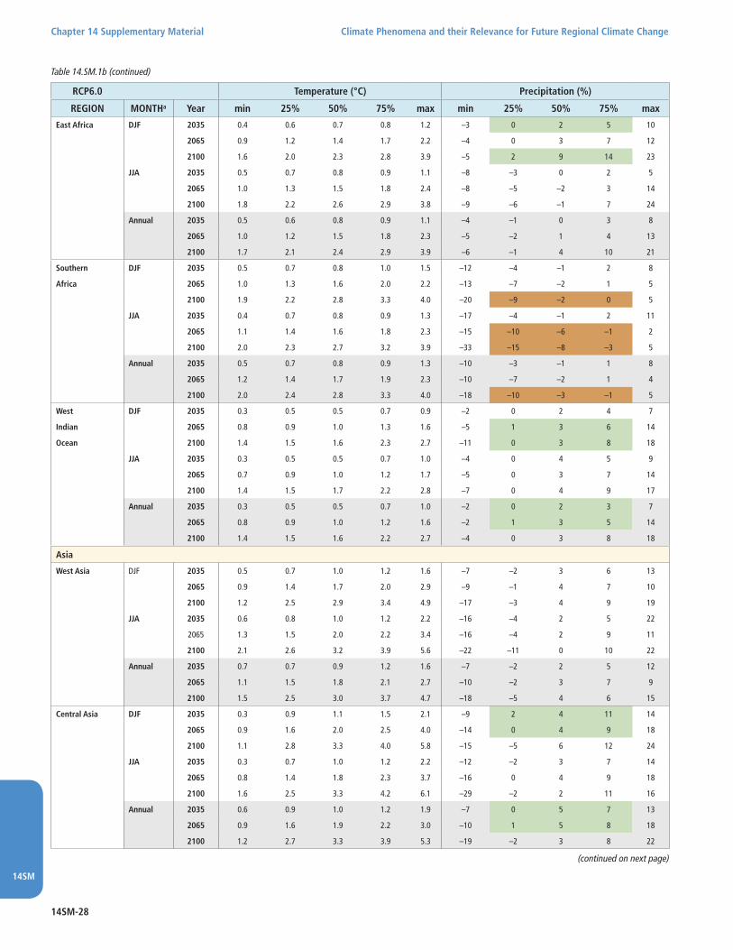
14SM-28
Chapter 14 Supplementary Material Climate Phenomena and their Relevance for Future Regional Climate Change
14SM
RCP6.0 Temperature (°C) Precipitation (%)
REGION MONTHa Year min 25% 50% 75% max min 25% 50% 75% max
East Africa DJF 2035 0.4 0.6 0.7 0.8 1.2 –3 0 2 5 10
2065 0.9 1.2 1.4 1.7 2.2 –4 0 3 7 12
2100 1.6 2.0 2.3 2.8 3.9 –5 2 9 14 23
JJA 2035 0.5 0.7 0.8 0.9 1.1 –8 –3 0 2 5
2065 1.0 1.3 1.5 1.8 2.4 –8 –5 –2 3 14
2100 1.8 2.2 2.6 2.9 3.8 –9 –6 –1 7 24
Annual 2035 0.5 0.6 0.8 0.9 1.1 –4 –1 0 3 8
2065 1.0 1.2 1.5 1.8 2.3 –5 –2 1 4 13
2100 1.7 2.1 2.4 2.9 3.9 –6 –1 4 10 21
Southern DJF 2035 0.5 0.7 0.8 1.0 1.5 –12 –4 –1 2 8
Africa 2065 1.0 1.3 1.6 2.0 2.2 –13 –7 –2 1 5
2100 1.9 2.2 2.8 3.3 4.0 –20 –9 –2 0 5
JJA 2035 0.4 0.7 0.8 0.9 1.3 –17 –4 –1 2 11
2065 1.1 1.4 1.6 1.8 2.3 –15 –10 –6 –1 2
2100 2.0 2.3 2.7 3.2 3.9 –33 –15 –8 –3 5
Annual 2035 0.5 0.7 0.8 0.9 1.3 –10 –3 –1 1 8
2065 1.2 1.4 1.7 1.9 2.3 –10 –7 –2 1 4
2100 2.0 2.4 2.8 3.3 4.0 –18 –10 –3 –1 5
West DJF 2035 0.3 0.5 0.5 0.7 0.9 –2 0 2 4 7
Indian 2065 0.8 0.9 1.0 1.3 1.6 –5 1 3 6 14
Ocean 2100 1.4 1.5 1.6 2.3 2.7 –11 0 3 8 18
JJA 2035 0.3 0.5 0.5 0.7 1.0 –4 0 4 5 9
2065 0.7 0.9 1.0 1.2 1.7 –5 0 3 7 14
2100 1.4 1.5 1.7 2.2 2.8 –7 0 4 9 17
Annual 2035 0.3 0.5 0.5 0.7 1.0 –2 0 2 3 7
2065 0.8 0.9 1.0 1.2 1.6 –2 1 3 5 14
2100 1.4 1.5 1.6 2.2 2.7 –4 0 3 8 18
Asia
West Asia DJF 2035 0.5 0.7 1.0 1.2 1.6 –7 –2 3 6 13
2065 0.9 1.4 1.7 2.0 2.9 –9 –1 4 7 10
2100 1.2 2.5 2.9 3.4 4.9 –17 –3 4 9 19
JJA 2035 0.6 0.8 1.0 1.2 2.2 –16 –4 2 5 22
2065 1.3 1.5 2.0 2.2 3.4 –16 –4 2 9 11
2100 2.1 2.6 3.2 3.9 5.6 –22 –11 0 10 22
Annual 2035 0.7 0.7 0.9 1.2 1.6 –7 –2 2 5 12
2065 1.1 1.5 1.8 2.1 2.7 –10 –2 3 7 9
2100 1.5 2.5 3.0 3.7 4.7 –18 –5 4 6 15
Central Asia DJF 2035 0.3 0.9 1.1 1.5 2.1 –9 2 4 11 14
2065 0.9 1.6 2.0 2.5 4.0 –14 0 4 9 18
2100 1.1 2.8 3.3 4.0 5.8 –15 –5 6 12 24
JJA 2035 0.3 0.7 1.0 1.2 2.2 –12 –2 3 7 14
2065 0.8 1.4 1.8 2.3 3.7 –16 0 4 9 18
2100 1.6 2.5 3.3 4.2 6.1 –29 –2 2 11 16
Annual 2035 0.6 0.9 1.0 1.2 1.9 –7 0 5 7 13
2065 0.9 1.6 1.9 2.2 3.0 –10 1 5 8 18
2100 1.2 2.7 3.3 3.9 5.3 –19 –2 3 8 22
(continued on next page)
Table 14.SM.1b (continued)

14SM-29
Climate Phenomena and their Relevance for Future Regional Climate Change Chapter 14 Supplementary Material
14SM
RCP6.0 Temperature (°C) Precipitation (%)
REGION MONTHa Year min 25% 50% 75% max min 25% 50% 75% max
Eastern Asia DJF 2035 0.0 0.8 1.0 1.3 2.0 –4 0 2 4 11
2065 0.5 1.5 1.9 2.3 3.1 –12 –1 3 5 13
2100 1.2 2.7 3.1 3.8 5.0 –7 4 8 12 19
JJA 2035 0.4 0.6 0.7 0.9 1.5 –3 1 2 4 6
2065 0.9 1.3 1.6 1.8 2.7 –3 1 2 5 7
2100 1.4 2.2 2.8 3.6 4.5 2 5 7 10 21
Annual 2035 0.4 0.7 0.9 1.1 1.4 –2 1 2 3 6
2065 0.9 1.5 1.6 1.9 2.7 –3 1 3 4 6
2100 1.2 2.3 2.9 3.5 4.5 0 5 8 10 18
Tibetan DJF 2035 0.3 0.8 1.1 1.5 2.1 0 3 6 8 13
Plateau 2065 0.9 1.7 2.0 2.6 3.5 –1 6 8 12 17
2100 1.7 2.9 3.4 4.3 5.8 1 7 12 18 30
JJA 2035 0.4 0.8 0.9 1.1 2.3 –3 1 3 6 15
2065 1.1 1.6 1.8 2.1 4.0 –4 3 6 9 23
2100 1.7 2.7 3.2 3.9 6.2 –4 5 9 14 40
Annual 2035 0.6 0.7 1.1 1.2 1.8 –1 2 4 6 13
2065 1.2 1.7 2.0 2.2 3.2 –2 5 6 10 20
2100 1.5 2.7 3.3 3.9 5.4 1 7 12 14 35
South Asia DJF 2035 0.3 0.6 0.9 1.1 1.3 –7 –1 5 8 14
2065 0.8 1.3 1.5 1.8 2.4 –9 –1 7 10 22
2100 1.9 2.3 2.7 3.3 3.9 –12 5 10 13 51
JJA 2035 0.2 0.5 0.7 0.8 1.1 –3 1 3 4 7
2065 0.7 1.0 1.3 1.5 2.2 –5 3 5 6 15
2100 1.6 1.9 2.2 2.8 3.8 –8 8 11 14 25
Annual 2035 0.3 0.6 0.8 0.9 1.2 –2 1 4 5 7
2065 1.1 1.2 1.3 1.7 2.0 –5 2 5 6 16
2100 1.9 2.2 2.4 3.3 3.8 –5 9 11 14 24
North DJF 2035 0.3 0.5 0.6 0.7 1.0 –7 –1 6 10 16
Indian 2065 0.7 0.9 1.0 1.3 1.6 –8 3 8 19 25
Ocean 2100 1.3 1.6 1.7 2.3 2.8 –7 8 14 27 57
JJA 2035 0.3 0.5 0.6 0.7 1.0 –6 –2 1 5 10
2065 0.8 0.9 1.1 1.3 1.7 –6 0 4 8 21
2100 1.5 1.6 1.8 2.3 2.9 –13 3 6 13 36
Annual 2035 0.3 0.5 0.6 0.7 1.0 –3 –1 3 6 12
2065 0.8 0.9 1.0 1.3 1.6 –4 2 6 9 23
2100 1.5 1.6 1.7 2.4 2.8 –7 3 12 15 47
Southeast DJF 2035 0.3 0.5 0.6 0.7 1.0 –8 –1 0 1 4
Asia (land) 2065 0.7 0.9 1.1 1.4 1.8 –6 –2 1 4 8
2100 1.3 1.7 1.8 2.4 3.2 –9 0 4 8 14
JJA 2035 0.4 0.5 0.6 0.7 1.1 –5 –2 0 2 5
2065 0.7 1.0 1.2 1.4 2.0 –5 –2 0 4 6
2100 1.5 1.8 1.9 2.4 3.4 –6 –1 4 8 13
Annual 2035 0.4 0.5 0.6 0.7 1.0 –6 –1 0 2 4
2065 0.8 1.0 1.1 1.4 1.8 –5 –1 1 4 7
2100 1.5 1.7 1.9 2.5 3.2 –4 0 3 8 14
(continued on next page)
Table 14.SM.1b (continued)

14SM-30
Chapter 14 Supplementary Material Climate Phenomena and their Relevance for Future Regional Climate Change
14SM
RCP6.0 Temperature (°C) Precipitation (%)
REGION MONTHa Year min 25% 50% 75% max min 25% 50% 75% max
Southeast DJF 2035 0.3 0.5 0.5 0.6 1.1 –3 –1 0 1 5
Asia (sea) 2065 0.7 0.8 1.0 1.2 1.7 –5 –1 2 4 7
2100 1.4 1.5 1.5 2.1 2.9 –5 0 3 6 14
JJA 2035 0.2 0.5 0.5 0.6 1.0 –4 0 1 2 5
2065 0.8 0.8 1.0 1.2 1.7 –4 0 2 4 9
2100 1.4 1.5 1.6 2.1 2.9 –4 2 3 5 13
Annual 2035 0.2 0.5 0.5 0.6 1.0 –3 0 1 2 3
2065 0.7 0.9 0.9 1.2 1.7 –2 –1 2 4 7
2100 1.4 1.5 1.6 2.1 2.8 –2 1 3 5 13
Australia
North DJF 2035 0.3 0.6 0.7 1.0 1.9 –17 –5 –3 1 9
Australia 2065 0.9 1.4 1.5 1.9 2.7 –16 –4 –1 3 10
2100 1.3 2.2 2.6 3.0 4.0 –30 –8 –1 6 18
JJA 2035 0.1 0.6 0.8 1.1 1.3 –36 –12 –5 2 17
2065 0.9 1.4 1.5 1.9 2.1 –46 –12 –3 2 14
2100 1.8 2.1 2.8 3.1 3.5 –57 –18 –4 5 15
Annual 2035 0.4 0.6 0.8 1.0 1.4 –14 –8 –3 1 9
2065 1.0 1.3 1.6 1.8 2.2 –18 –5 –1 3 9
2100 1.5 2.3 2.7 3.1 3.6 –29 –9 0 3 15
South Australia/ DJF 2035 0.5 0.6 0.7 0.9 1.4 –22 –5 –1 1 6
New Zealand 2065 0.8 1.3 1.4 1.6 2.1 –24 –6 –1 3 10
2100 1.6 1.9 2.3 2.9 3.7 –19 –5 –1 2 11
JJA 2035 0.4 0.5 0.7 0.7 0.9 –16 –4 –1 1 4
2065 0.6 1.0 1.2 1.4 1.6 –27 –6 –1 2 5
2100 1.3 1.7 2.1 2.3 2.8 –28 –9 –2 3 10
Annual 2035 0.5 0.6 0.7 0.8 1.0 –17 –3 –1 0 5
2065 0.9 1.1 1.4 1.5 1.7 –24 –4 –1 3 4
2100 1.5 1.9 2.3 2.5 2.9 –23 –5 –1 2 9
The Pacific
Northern DJF 2035 0.3 0.4 0.5 0.6 0.9 –4 –1 0 2 7
Tropical 2065 0.7 0.8 1.0 1.2 1.6 –5 –1 2 4 7
Pacific 2100 1.2 1.5 1.7 2.2 2.8 –9 –1 2 6 13
JJA 2035 0.3 0.4 0.5 0.6 1.0 –7 –2 1 3 6
2065 0.7 0.9 0.9 1.2 1.8 –5 –1 1 4 6
2100 1.3 1.4 1.6 2.3 3.0 –10 –2 2 6 12
Annual 2035 0.3 0.5 0.5 0.6 0.9 –4 –2 0 2 6
2065 0.7 0.9 1.0 1.2 1.7 –4 –1 1 3 6
2100 1.3 1.4 1.7 2.3 2.9 –9 0 2 5 9
Equatorial DJF 2035 0.4 0.5 0.6 0.8 1.0 –2 1 6 14 41
Pacific 2065 0.5 1.0 1.1 1.4 1.9 –6 9 14 20 133
2100 1.0 1.6 1.8 2.4 3.3 –11 7 18 32 250
JJA 2035 0.4 0.5 0.6 0.7 1.1 –1 5 9 13 21
2065 0.7 0.9 1.1 1.3 2.1 –15 11 16 25 87
2100 1.2 1.5 1.8 2.3 3.4 –3 21 29 42 164
Annual 2035 0.4 0.5 0.6 0.7 0.9 –1 5 7 12 33
2065 0.6 1.0 1.1 1.3 1.9 –1 9 14 21 113
2100 1.2 1.6 1.8 2.3 3.1 –5 16 22 31 215
(continued on next page)
Table 14.SM.1b (continued)
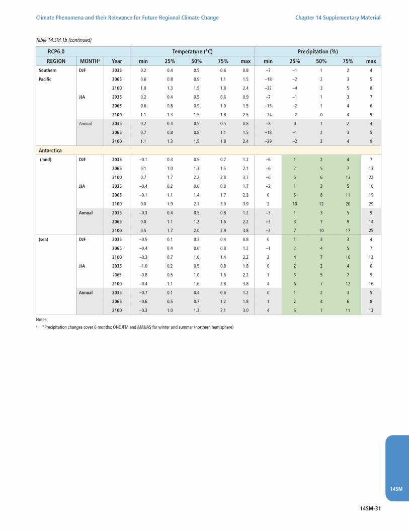
14SM-31
Climate Phenomena and their Relevance for Future Regional Climate Change Chapter 14 Supplementary Material
14SM
RCP6.0 Temperature (°C) Precipitation (%)
REGION MONTHa Year min 25% 50% 75% max min 25% 50% 75% max
Southern DJF 2035 0.2 0.4 0.5 0.6 0.8 –7 –1 1 2 4
Pacific 2065 0.6 0.8 0.9 1.1 1.5 –18 –2 2 3 5
2100 1.0 1.3 1.5 1.8 2.4 –32 –4 3 5 8
JJA 2035 0.2 0.4 0.5 0.6 0.9 –7 –1 1 3 7
2065 0.6 0.8 0.9 1.0 1.5 –15 –2 1 4 6
2100 1.1 1.3 1.5 1.8 2.5 –24 –2 0 4 9
Annual 2035 0.2 0.4 0.5 0.5 0.8 –8 0 1 2 4
2065 0.7 0.8 0.8 1.1 1.5 –18 –1 2 3 5
2100 1.1 1.3 1.5 1.8 2.4 –29 –2 2 4 9
Antarctica
(land) DJF 2035 –0.1 0.3 0.5 0.7 1.2 –6 1 2 4 7
2065 0.1 1.0 1.3 1.5 2.1 –6 2 5 7 13
2100 0.7 1.7 2.2 2.8 3.7 –6 5 6 13 22
JJA 2035 –0.4 0.2 0.6 0.8 1.7 –2 1 3 5 10
2065 –0.1 1.1 1.4 1.7 2.2 0 5 8 11 15
2100 0.0 1.9 2.1 3.0 3.9 2 10 12 20 29
Annual 2035 –0.3 0.4 0.5 0.8 1.2 –3 1 3 5 9
2065 0.0 1.1 1.2 1.6 2.2 –3 3 7 9 14
2100 0.5 1.7 2.0 2.9 3.8 –2 7 10 17 25
(sea) DJF 2035 –0.5 0.1 0.3 0.4 0.8 0 1 3 3 4
2065 –0.4 0.4 0.6 0.8 1.2 –1 2 4 5 7
2100 –0.3 0.7 1.0 1.4 2.2 2 4 7 10 12
JJA 2035 –1.0 0.2 0.5 0.8 1.8 0 2 2 4 6
2065 –0.8 0.5 1.0 1.6 2.2 1 3 5 7 9
2100 –0.4 1.1 1.6 2.8 3.8 4 6 7 12 16
Annual 2035 –0.7 0.1 0.4 0.6 1.2 0 1 2 3 5
2065 –0.6 0.5 0.7 1.2 1.8 1 2 4 6 8
2100 –0.3 1.0 1.3 2.1 3.0 4 5 7 11 13
Table 14.SM.1b (continued)
Notes:a *Precipitation changes cover 6 months; ONDJFM and AMJJAS for winter and summer (northern hemisphere)
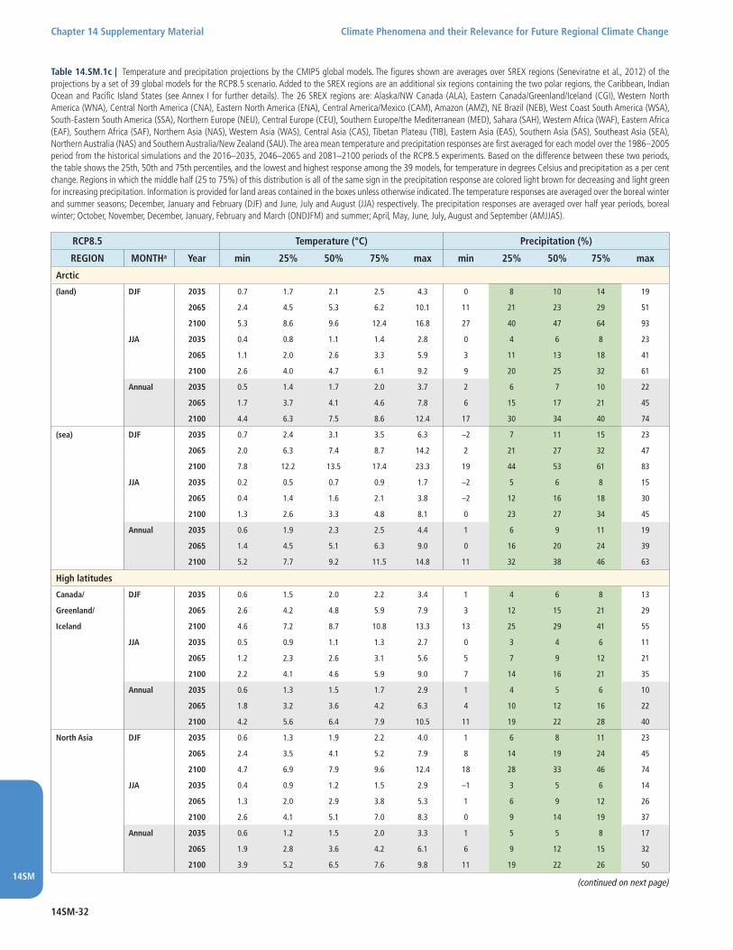
14SM-32
Chapter 14 Supplementary Material Climate Phenomena and their Relevance for Future Regional Climate Change
14SM
RCP8.5 Temperature (°C) Precipitation (%)
REGION MONTHa Year min 25% 50% 75% max min 25% 50% 75% max
Arctic
(land) DJF 2035 0.7 1.7 2.1 2.5 4.3 0 8 10 14 19
2065 2.4 4.5 5.3 6.2 10.1 11 21 23 29 51
2100 5.3 8.6 9.6 12.4 16.8 27 40 47 64 93
JJA 2035 0.4 0.8 1.1 1.4 2.8 0 4 6 8 23
2065 1.1 2.0 2.6 3.3 5.9 3 11 13 18 41
2100 2.6 4.0 4.7 6.1 9.2 9 20 25 32 61
Annual 2035 0.5 1.4 1.7 2.0 3.7 2 6 7 10 22
2065 1.7 3.7 4.1 4.6 7.8 6 15 17 21 45
2100 4.4 6.3 7.5 8.6 12.4 17 30 34 40 74
(sea) DJF 2035 0.7 2.4 3.1 3.5 6.3 –2 7 11 15 23
2065 2.0 6.3 7.4 8.7 14.2 2 21 27 32 47
2100 7.8 12.2 13.5 17.4 23.3 19 44 53 61 83
JJA 2035 0.2 0.5 0.7 0.9 1.7 –2 5 6 8 15
2065 0.4 1.4 1.6 2.1 3.8 –2 12 16 18 30
2100 1.3 2.6 3.3 4.8 8.1 0 23 27 34 45
Annual 2035 0.6 1.9 2.3 2.5 4.4 1 6 9 11 19
2065 1.4 4.5 5.1 6.3 9.0 0 16 20 24 39
2100 5.2 7.7 9.2 11.5 14.8 11 32 38 46 63
High latitudes
Canada/ DJF 2035 0.6 1.5 2.0 2.2 3.4 1 4 6 8 13
Greenland/ 2065 2.6 4.2 4.8 5.9 7.9 3 12 15 21 29
Iceland 2100 4.6 7.2 8.7 10.8 13.3 13 25 29 41 55
JJA 2035 0.5 0.9 1.1 1.3 2.7 0 3 4 6 11
2065 1.2 2.3 2.6 3.1 5.6 5 7 9 12 21
2100 2.2 4.1 4.6 5.9 9.0 7 14 16 21 35
Annual 2035 0.6 1.3 1.5 1.7 2.9 1 4 5 6 10
2065 1.8 3.2 3.6 4.2 6.3 4 10 12 16 22
2100 4.2 5.6 6.4 7.9 10.5 11 19 22 28 40
North Asia DJF 2035 0.6 1.3 1.9 2.2 4.0 1 6 8 11 23
2065 2.4 3.5 4.1 5.2 7.9 8 14 19 24 45
2100 4.7 6.9 7.9 9.6 12.4 18 28 33 46 74
JJA 2035 0.4 0.9 1.2 1.5 2.9 –1 3 5 6 14
2065 1.3 2.0 2.9 3.8 5.3 1 6 9 12 26
2100 2.6 4.1 5.1 7.0 8.3 0 9 14 19 37
Annual 2035 0.6 1.2 1.5 2.0 3.3 1 5 5 8 17
2065 1.9 2.8 3.6 4.2 6.1 6 9 12 15 32
2100 3.9 5.2 6.5 7.6 9.8 11 19 22 26 50
Table 14.SM.1c | Temperature and precipitation projections by the CMIP5 global models. The figures shown are averages over SREX regions (Seneviratne et al., 2012) of the projections by a set of 39 global models for the RCP8.5 scenario. Added to the SREX regions are an additional six regions containing the two polar regions, the Caribbean, Indian Ocean and Pacific Island States (see Annex I for further details). The 26 SREX regions are: Alaska/NW Canada (ALA), Eastern Canada/Greenland/Iceland (CGI), Western North America (WNA), Central North America (CNA), Eastern North America (ENA), Central America/Mexico (CAM), Amazon (AMZ), NE Brazil (NEB), West Coast South America (WSA), South-Eastern South America (SSA), Northern Europe (NEU), Central Europe (CEU), Southern Europe/the Mediterranean (MED), Sahara (SAH), Western Africa (WAF), Eastern Africa (EAF), Southern Africa (SAF), Northern Asia (NAS), Western Asia (WAS), Central Asia (CAS), Tibetan Plateau (TIB), Eastern Asia (EAS), Southern Asia (SAS), Southeast Asia (SEA), Northern Australia (NAS) and Southern Australia/New Zealand (SAU). The area mean temperature and precipitation responses are first averaged for each model over the 1986–2005 period from the historical simulations and the 2016–2035, 2046–2065 and 2081–2100 periods of the RCP8.5 experiments. Based on the difference between these two periods, the table shows the 25th, 50th and 75th percentiles, and the lowest and highest response among the 39 models, for temperature in degrees Celsius and precipitation as a per cent change. Regions in which the middle half (25 to 75%) of this distribution is all of the same sign in the precipitation response are colored light brown for decreasing and light green for increasing precipitation. Information is provided for land areas contained in the boxes unless otherwise indicated. The temperature responses are averaged over the boreal winter and summer seasons; December, January and February (DJF) and June, July and August (JJA) respectively. The precipitation responses are averaged over half year periods, boreal winter; October, November, December, January, February and March (ONDJFM) and summer; April, May, June, July, August and September (AMJJAS).
(continued on next page)

14SM-33
Climate Phenomena and their Relevance for Future Regional Climate Change Chapter 14 Supplementary Material
14SM
RCP8.5 Temperature (°C) Precipitation (%)
REGION MONTHa Year min 25% 50% 75% max min 25% 50% 75% max
North America
Alaska/ DJF 2035 –0.8 1.6 2.1 3.2 4.8 –5 4 6 11 17
NW Canada 2065 2.9 4.5 5.1 6.3 8.8 2 10 17 21 37
2100 5.3 7.7 9.3 11.8 14.8 12 22 33 43 73
JJA 2035 0.2 0.8 1.2 1.5 2.6 –1 3 6 7 16
2065 0.9 2.0 2.7 3.4 5.4 4 10 13 14 32
2100 2.3 3.8 4.9 6.0 8.3 10 17 23 27 47
Annual 2035 0.4 1.3 1.7 2.3 3.0 –2 4 5 8 16
2065 2.3 3.3 3.7 4.6 6.1 7 10 14 18 32
2100 4.1 5.6 6.9 8.5 10.5 11 23 26 32 51
West North DJF 2035 0.2 1.0 1.3 1.7 2.5 –4 1 3 4 8
America 2065 1.0 2.5 3.0 3.4 5.0 –2 3 6 8 20
2100 2.7 4.1 5.0 6.1 8.7 –3 8 12 13 27
JJA 2035 0.6 1.0 1.3 1.5 2.2 –4 0 2 3 8
2065 1.6 2.3 2.9 3.7 4.4 –7 –1 2 4 15
2100 3.5 4.7 5.2 6.5 7.8 –16 –4 0 5 20
Annual 2035 0.5 1.0 1.2 1.5 2.0 –2 1 2 4 7
2065 1.7 2.4 2.8 3.4 4.2 –2 1 4 6 18
2100 3.1 4.2 5.0 6.1 7.7 –2 3 6 8 25
Central DJF 2035 0.0 1.0 1.2 1.7 2.3 –6 –2 2 6 11
North 2065 1.1 2.2 2.7 3.6 4.8 –12 1 7 10 17
America 2100 2.9 4.1 5.0 5.9 7.7 –18 4 11 17 28
JJA 2035 0.5 1.1 1.2 1.4 2.3 –9 –2 1 3 9
2065 1.7 2.3 2.9 3.4 4.6 –19 –1 3 6 13
2100 3.6 4.6 5.4 6.2 8.0 –19 –4 3 7 16
Annual 2035 0.6 1.0 1.2 1.5 2.0 –5 –1 2 4 10
2065 1.7 2.4 2.8 3.3 4.2 –10 1 4 7 15
2100 3.4 4.4 5.1 5.7 7.4 –14 0 7 9 16
Eastern DJF 2035 0.0 0.9 1.4 1.6 2.7 –3 1 4 6 11
North 2065 1.8 2.4 3.0 3.7 5.1 –1 6 9 15 20
America 2100 3.2 4.6 5.5 6.4 8.6 –2 12 17 24 32
JJA 2035 0.4 0.9 1.1 1.4 2.3 –7 1 3 5 10
2065 1.4 2.4 2.8 3.3 4.8 –8 2 5 7 12
2100 2.8 4.2 5.1 5.9 8.3 –11 1 7 9 25
Annual 2035 0.4 0.9 1.2 1.4 2.1 –3 1 4 5 7
2065 1.7 2.5 2.8 3.3 4.5 1 4 7 10 14
2100 3.5 4.3 5.1 6.0 7.6 0 6 11 15 22
Central America
Central DJF 2035 0.5 0.7 0.9 1.0 1.3 –12 –4 0 3 13
America 2065 1.4 1.9 2.1 2.4 2.9 –17 –6 –2 1 12
2100 2.3 3.3 3.9 4.6 5.3 –27 –11 –5 4 13
JJA 2035 0.6 0.8 0.9 1.1 1.5 –14 –4 –1 3 9
2065 1.6 2.0 2.3 2.6 3.2 –14 –7 –5 0 11
2100 2.9 3.6 4.2 5.1 6.0 –27 –14 –11 –1 16
Annual 2035 0.5 0.8 0.9 1.1 1.4 –11 –3 –1 3 6
2065 1.5 1.9 2.1 2.6 3.0 –14 –7 –5 1 7
2100 2.9 3.5 3.9 4.9 5.5 –26 –12 –8 0 11
(continued on next page)
Table 14.SM.1c (continued)

14SM-34
Chapter 14 Supplementary Material Climate Phenomena and their Relevance for Future Regional Climate Change
14SM
RCP8.5 Temperature (°C) Precipitation (%)
REGION MONTHa Year min 25% 50% 75% max min 25% 50% 75% max
Caribbean DJF 2035 0.3 0.6 0.7 0.9 1.1 –11 –3 0 5 7
(land and sea) 2065 1.0 1.4 1.6 1.9 2.4 –13 –5 –1 3 10
2100 2.0 2.5 3.0 3.6 4.0 –39 –13 –5 3 19
JJA 2035 0.3 0.6 0.7 0.8 1.2 –17 –9 –6 –2 16
2065 1.2 1.4 1.6 1.9 2.5 –34 –24 –12 –5 13
2100 2.2 2.4 2.9 3.4 4.2 –60 –39 –24 –17 2
Annual 2035 0.4 0.6 0.7 0.9 1.1 –14 –5 –2 –1 11
2065 1.1 1.4 1.6 1.9 2.5 –19 –14 –8 –2 10
2100 2.1 2.5 3.0 3.6 4.1 –50 –23 –16 –7 9
South America
Amazon DJF 2035 0.5 0.8 0.9 1.1 1.8 –12 –4 –1 1 5
2065 1.3 1.9 2.3 2.8 3.9 –20 –6 –1 2 7
2100 1.9 3.5 4.3 5.3 6.3 –26 –11 –3 3 16
JJA 2035 0.5 0.8 1.0 1.2 2.1 –17 –3 –1 1 6
2065 1.5 2.1 2.6 2.9 4.2 –28 –6 –2 2 13
2100 3.0 3.8 4.7 5.7 7.6 –44 –11 –5 1 12
Annual 2035 0.5 0.8 1.1 1.2 1.9 –12 –3 –1 1 4
2065 1.4 2.0 2.5 2.8 4.1 –23 –5 –1 2 8
2100 2.4 3.7 4.3 5.7 7.0 –33 –11 –2 1 14
Northeast DJF 2035 0.5 0.7 0.9 1.1 1.5 –13 –6 –1 3 9
Brazil 2065 1.2 1.8 2.1 2.4 3.2 –16 –9 0 4 39
2100 2.1 3.4 3.8 4.6 5.6 –29 –11 –4 5 48
JJA 2035 0.4 0.7 0.9 1.1 1.3 –22 –10 –4 1 17
2065 1.2 1.8 2.2 2.5 3.1 –24 –13 –8 –3 32
2100 2.6 3.6 4.1 4.8 5.7 –41 –25 –18 –5 37
Annual 2035 0.5 0.8 1.0 1.1 1.5 –14 –6 0 2 7
2065 1.3 1.9 2.2 2.6 3.1 –16 –10 –2 1 38
2100 2.5 3.5 4.1 4.8 5.6 –31 –14 –6 6 45
West Coast DJF 2035 0.4 0.7 0.8 1.0 1.3 –5 0 1 3 6
South America 2065 1.6 1.8 2.1 2.4 2.9 –8 –1 2 4 10
2100 2.6 3.2 3.8 4.7 5.2 –11 1 3 7 14
JJA 2035 0.5 0.8 0.9 1.0 1.4 –9 –2 0 2 6
2065 1.5 1.9 2.2 2.5 3.0 –13 –3 –1 3 8
2100 2.9 3.3 3.8 4.8 5.3 –20 –6 –1 3 12
Annual 2035 0.5 0.7 0.9 1.0 1.4 –6 –1 1 2 5
2065 1.5 1.8 2.1 2.4 2.9 –9 –1 1 3 8
2100 2.8 3.3 3.8 4.8 5.1 –14 –1 1 6 11
Southeastern DJF 2035 0.1 0.6 0.8 1.0 1.5 –4 –1 2 4 13
South America 2065 1.0 1.7 1.9 2.2 3.5 –7 –1 3 7 14
2100 1.9 3.0 3.8 4.4 6.2 –10 1 6 11 24
JJA 2035 0.2 0.5 0.7 0.9 1.2 –12 –1 1 4 22
2065 0.9 1.5 1.8 2.1 2.7 –21 –2 4 8 27
2100 1.9 2.8 3.4 3.9 4.6 –24 –3 7 21 41
Annual 2035 0.2 0.6 0.8 0.9 1.4 –6 0 1 3 14
2065 1.1 1.7 1.9 2.2 3.1 –11 –1 3 8 18
2100 1.9 3.0 3.6 4.2 5.3 –11 1 7 14 27
Table 14.SM.1c (continued)
(continued on next page)

14SM-35
Climate Phenomena and their Relevance for Future Regional Climate Change Chapter 14 Supplementary Material
14SM
RCP8.5 Temperature (°C) Precipitation (%)
REGION MONTHa Year min 25% 50% 75% max min 25% 50% 75% max
Europe
Northern DJF 2035 –0.1 1.1 1.5 2.4 3.5 –3 3 5 7 16
Europe 2065 –0.6 2.9 3.4 4.7 6.8 2 8 11 15 26
2100 2.6 5.3 6.1 7.5 10.4 8 15 20 29 42
JJA 2035 0.3 0.8 1.1 1.5 2.8 –4 1 4 7 9
2065 0.1 1.9 2.5 3.2 4.9 –8 1 4 10 19
2100 2.1 3.5 4.5 5.8 7.6 –17 2 8 12 26
Annual 2035 0.3 0.9 1.2 1.8 2.7 –3 3 4 6 12
2065 –0.4 2.4 2.9 3.5 4.7 –2 6 8 11 23
2100 1.9 4.3 5.0 6.3 7.7 –2 12 14 18 34
Central Europe DJF 2035 –0.3 0.6 1.0 1.8 3.3 –7 1 4 6 15
2065 1.2 2.1 2.6 3.8 5.8 1 4 7 11 19
2100 3.4 4.2 4.9 5.9 8.2 –4 7 11 18 29
JJA 2035 0.4 1.0 1.3 1.6 2.8 –8 –2 1 5 8
2065 1.3 2.3 2.7 3.6 5.5 –18 –6 –2 4 10
2100 2.8 4.3 5.3 6.6 8.5 –28 –16 –8 –2 11
Annual 2035 0.5 0.9 1.1 1.6 2.5 –4 0 3 5 11
2065 1.0 2.2 2.7 3.3 4.6 –5 0 3 6 10
2100 3.1 4.0 4.8 5.8 7.1 –8 –3 0 7 14
Southern Europe/ DJF 2035 0.0 0.6 0.9 1.1 1.7 –10 –4 –1 1 8
Mediterranean 2065 0.7 1.8 2.2 2.7 3.1 –24 –9 –4 –2 6
2100 2.4 3.3 3.8 4.6 5.7 –35 –18 –12 –7 0
JJA 2035 0.6 1.1 1.4 1.6 2.7 –15 –7 –3 1 8
2065 2.1 2.6 3.3 3.7 5.6 –31 –18 –12 –7 9
2100 3.9 4.9 6.0 6.8 9.3 –58 –35 –24 –17 –4
Annual 2035 0.4 1.0 1.1 1.3 2.0 –8 –4 –2 0 5
2065 1.6 2.3 2.5 3.0 4.1 –23 –11 –7 –5 1
2100 3.3 4.1 4.5 5.6 6.9 –35 –23 –19 –13 –2
Africa
Sahara DJF 2035 0.2 0.9 1.1 1.2 1.6 –35 –13 –1 8 67
2065 1.3 2.2 2.5 2.9 3.2 –35 –15 –2 15 128
2100 3.2 3.8 4.4 5.3 6.4 –49 –26 –10 19 319
JJA 2035 0.4 1.0 1.2 1.4 2.0 –24 –3 6 19 34
2065 1.9 2.5 2.9 3.3 4.5 –23 –7 5 16 98
2100 3.4 4.6 5.0 6.5 7.8 –41 –14 9 25 147
Annual 2035 0.5 1.0 1.1 1.3 1.7 –25 –3 5 13 28
2065 1.8 2.4 2.7 3.2 3.7 –18 –8 4 13 84
2100 3.8 4.3 4.6 6.1 6.5 –42 –15 –2 18 155
West Africa DJF 2035 0.5 0.8 1.0 1.1 1.6 –6 0 2 4 8
2065 1.5 2.0 2.3 2.7 3.4 –2 2 4 9 13
2100 3.1 3.7 4.0 4.9 6.1 –8 3 7 13 23
JJA 2035 0.6 0.8 0.8 1.0 1.5 –6 –1 1 2 8
2065 1.6 1.9 2.0 2.8 3.3 –10 –1 1 4 9
2100 2.2 3.5 3.9 5.3 5.9 –13 –2 2 6 13
Annual 2035 0.7 0.8 0.9 1.1 1.5 –4 0 1 3 8
2065 1.6 1.9 2.1 2.7 3.3 –8 1 2 6 8
2100 2.6 3.6 4.0 5.1 5.9 –10 0 5 8 16
Table 14.SM.1c (continued)
(continued on next page)

14SM-36
Chapter 14 Supplementary Material Climate Phenomena and their Relevance for Future Regional Climate Change
14SM
RCP8.5 Temperature (°C) Precipitation (%)
REGION MONTHa Year min 25% 50% 75% max min 25% 50% 75% max
East Africa DJF 2035 0.6 0.8 0.9 1.1 1.6 –5 –1 2 6 10
2065 1.3 1.8 2.2 2.5 3.2 –8 1 6 12 23
2100 2.8 3.4 3.9 4.6 5.6 –11 6 15 22 35
JJA 2035 0.6 0.8 0.9 1.2 1.5 –8 –4 –1 3 11
2065 1.3 2.0 2.1 2.8 3.2 –12 –6 0 5 21
2100 1.8 3.5 4.1 5.2 5.6 –15 –5 4 13 33
Annual 2035 0.6 0.7 0.9 1.1 1.5 –6 –2 0 3 9
2065 1.6 1.9 2.2 2.7 3.2 –9 –1 4 7 20
2100 2.4 3.5 4.0 5.0 5.6 –11 0 11 16 34
Southern DJF 2035 0.5 0.8 1.0 1.2 1.5 –10 –4 –2 0 5
Africa 2065 1.5 2.0 2.5 2.8 3.3 –19 –8 –4 –1 5
2100 3.1 3.8 4.4 5.2 6.2 –26 –12 –5 –3 2
JJA 2035 0.5 0.8 1.0 1.1 1.6 –19 –9 –4 –1 5
2065 1.9 2.1 2.4 2.7 3.3 –31 –18 –11 –6 6
2100 3.3 4.0 4.5 5.2 6.1 –48 –27 –18 –13 1
Annual 2035 0.6 0.9 1.1 1.2 1.6 –11 –4 –2 0 2
2065 1.7 2.2 2.5 2.9 3.4 –19 –9 –5 –2 5
2100 3.3 4.1 4.5 5.5 6.3 –24 –14 –9 –5 3
West Indian DJF 2035 0.3 0.6 0.7 0.8 1.1 –4 –1 0 3 10
Ocean 2065 1.1 1.4 1.6 1.9 2.2 –6 –2 2 5 17
2100 2.1 2.6 2.9 3.5 4.1 –10 –1 4 11 25
JJA 2035 0.3 0.6 0.7 0.8 1.2 –8 –2 2 5 9
2065 1.0 1.4 1.6 1.8 2.2 –13 –1 2 5 17
2100 1.7 2.5 2.9 3.5 4.3 –10 –1 4 7 24
Annual 2035 0.3 0.6 0.7 0.7 1.1 –3 0 1 3 9
2065 1.1 1.4 1.5 1.8 2.2 –7 –1 1 5 16
2100 2.0 2.6 2.9 3.5 4.2 –6 –2 4 9 24
Asia
West Asia DJF 2035 0.5 0.8 1.2 1.4 1.9 –10 –2 4 6 19
2065 1.1 2.2 2.6 3.2 4.1 –14 0 3 6 36
2100 3.1 4.0 4.6 5.6 6.8 –17 –2 4 9 45
JJA 2035 0.5 1.0 1.2 1.4 2.4 –10 –4 1 7 24
2065 1.8 2.6 3.1 3.6 4.8 –23 –7 –4 5 52
2100 3.8 4.6 5.3 6.6 8.2 –38 –15 –8 11 84
Annual 2035 0.5 1.0 1.1 1.4 2.0 –8 –2 3 7 22
2065 1.6 2.5 2.8 3.4 4.1 –14 –5 0 6 24
2100 3.7 4.5 5.0 6.2 6.9 –21 –7 –1 8 40
Central Asia DJF 2035 0.4 0.9 1.3 1.6 2.6 –11 0 3 7 17
2065 0.8 2.4 3.0 3.6 5.6 –13 –3 3 13 31
2100 3.5 4.3 5.3 6.3 8.0 –20 –5 7 14 41
JJA 2035 0.5 1.0 1.3 1.6 2.4 –15 –1 4 9 24
2065 1.9 2.4 3.0 3.7 5.1 –27 –5 1 8 18
2100 3.2 4.5 5.7 6.5 8.6 –30 –7 1 6 26
Annual 2035 0.4 1.0 1.3 1.5 2.1 –9 –2 3 9 16
2065 1.7 2.5 3.1 3.4 4.4 –14 –3 4 8 21
2100 3.7 4.6 5.3 6.3 7.6 –20 –6 2 11 35
Table 14.SM.1c (continued)
(continued on next page)

14SM-37
Climate Phenomena and their Relevance for Future Regional Climate Change Chapter 14 Supplementary Material
14SM
RCP8.5 Temperature (°C) Precipitation (%)
REGION MONTHa Year min 25% 50% 75% max min 25% 50% 75% max
Eastern Asia DJF 2035 0.1 0.9 1.2 1.5 2.4 –7 –1 1 3 14
2065 1.3 2.3 2.9 3.3 4.7 –10 3 6 9 23
2100 3.5 4.2 5.4 6.1 7.5 –15 9 13 19 32
JJA 2035 0.5 0.9 1.0 1.2 1.9 –4 0 1 3 5
2065 1.4 2.1 2.6 3.1 3.9 –3 3 6 9 15
2100 2.8 3.8 4.8 5.7 6.8 1 7 9 15 28
Annual 2035 0.5 0.9 1.1 1.3 1.9 –2 0 1 3 5
2065 1.6 2.2 2.7 3.1 4.2 –1 4 6 9 14
2100 3.3 4.0 4.9 5.6 7.2 –3 7 10 16 22
Tibetan DJF 2035 0.2 1.1 1.3 1.7 2.4 –2 2 5 7 12
Plateau 2065 1.6 2.6 3.2 3.8 5.3 –1 8 13 16 26
2100 3.9 4.8 5.8 7.0 9.1 0 15 20 28 46
JJA 2035 0.6 1.0 1.2 1.4 2.5 –3 2 4 6 14
2065 1.8 2.4 2.9 3.3 5.3 –2 5 8 11 32
2100 3.6 4.6 5.3 6.0 8.8 –3 8 13 18 55
Annual 2035 0.6 1.0 1.3 1.5 2.0 –2 3 4 5 13
2065 1.9 2.5 3.0 3.5 4.8 –2 6 9 12 28
2100 3.9 4.7 5.5 6.3 8.4 –2 10 16 21 47
South Asia DJF 2035 0.3 0.8 1.0 1.2 1.6 –13 –2 1 6 20
2065 1.5 2.2 2.6 3.0 3.7 –16 –4 4 10 23
2100 3.5 4.1 4.6 5.7 7.1 –17 –1 12 21 42
JJA 2035 0.3 0.6 0.8 1.0 1.3 –3 1 3 5 16
2065 1.2 1.7 2.0 2.3 3.3 –1 7 10 13 27
2100 1.3 3.0 3.7 4.6 5.6 –9 13 17 23 57
Annual 2035 0.4 0.8 0.9 1.0 1.4 –2 1 3 5 11
2065 1.5 2.0 2.2 2.6 3.1 0 6 8 11 17
2100 3.1 3.7 4.1 5.2 6.0 –7 11 18 21 45
North Indian DJF 2035 0.3 0.6 0.7 0.8 1.0 –10 0 5 8 22
Ocean 2065 0.9 1.5 1.6 2.0 2.5 –18 3 13 21 44
2100 2.1 2.7 3.0 3.9 4.5 –7 9 19 34 65
JJA 2035 0.3 0.6 0.7 0.8 1.1 –10 0 3 5 10
2065 1.0 1.5 1.6 2.0 2.4 –7 3 6 11 29
2100 1.9 2.7 3.0 3.6 4.3 –14 7 14 20 52
Annual 2035 0.3 0.6 0.7 0.8 1.0 –4 2 3 5 16
2065 1.0 1.5 1.6 2.0 2.4 –5 3 7 14 29
2100 2.1 2.7 3.0 3.8 4.3 –9 8 18 23 56
Southeast DJF 2035 0.3 0.6 0.7 0.9 1.2 –6 0 2 4 10
Asia (land) 2065 1.1 1.5 1.8 2.2 2.7 –3 1 5 10 19
2100 2.1 2.9 3.2 4.2 4.9 –8 2 8 19 31
JJA 2035 0.4 0.6 0.7 0.9 1.3 –4 –1 0 2 7
2065 1.1 1.6 1.8 2.1 2.8 –5 0 5 9 17
2100 2.1 2.9 3.3 4.2 5.1 –8 –1 7 16 30
Annual 2035 0.3 0.6 0.8 0.9 1.2 –4 0 1 3 8
2065 1.1 1.6 1.7 2.2 2.7 –3 0 5 10 17
2100 2.1 3.0 3.2 4.4 4.9 –7 0 8 19 29
Table 14.SM.1c (continued)
(continued on next page)
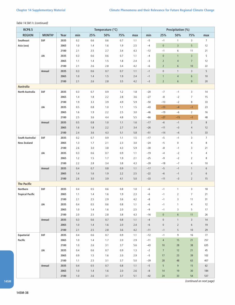
14SM-38
Chapter 14 Supplementary Material Climate Phenomena and their Relevance for Future Regional Climate Change
14SM
RCP8.5 Temperature (°C) Precipitation (%)
REGION MONTHa Year min 25% 50% 75% max min 25% 50% 75% max
Southeast DJF 2035 0.2 0.6 0.6 0.7 1.1 –5 –1 1 3 7
Asia (sea) 2065 1.0 1.4 1.6 1.9 2.5 –4 0 3 5 12
2100 2.1 2.5 2.7 3.4 4.3 –12 –1 6 11 21
JJA 2035 0.3 0.6 0.6 0.7 1.1 –4 0 1 3 5
2065 1.1 1.4 1.5 1.8 2.4 –3 2 4 7 12
2100 2.1 2.6 2.8 3.4 4.2 –6 2 6 10 22
Annual 2035 0.3 0.6 0.7 0.7 1.1 –1 0 1 3 5
2065 1.0 1.4 1.5 1.9 2.4 –1 1 4 6 10
2100 2.1 2.6 2.8 3.5 4.2 –3 2 6 9 20
Australia
North Australia DJF 2035 0.3 0.7 0.9 1.2 1.8 –20 –7 –1 3 14
2065 1.4 1.8 2.2 2.8 3.6 –27 –8 –2 7 15
2100 1.9 3.3 3.9 4.9 5.9 –50 –13 –2 8 33
JJA 2035 0.5 0.8 1.0 1.1 1.5 –43 –13 –4 –1 23
2065 1.6 1.9 2.2 2.5 3.0 –46 –19 –6 2 16
2100 2.5 3.6 4.4 4.8 5.5 –66 –27 –15 –1 48
Annual 2035 0.5 0.8 1.0 1.1 1.6 –17 –6 –1 2 8
2065 1.6 1.8 2.2 2.7 3.4 –26 –11 –3 4 12
2100 2.4 3.6 4.3 5.1 5.8 –51 –14 –4 5 33
South Australia/ DJF 2035 0.2 0.7 0.9 1.1 1.5 –17 –5 –1 3 7
New Zealand 2065 1.3 1.7 2.1 2.3 3.0 –24 –5 0 4 8
2100 2.6 3.0 3.8 4.3 5.9 –30 –8 –1 3 21
JJA 2035 0.3 0.6 0.7 0.9 1.1 –19 –4 –2 1 4
2065 1.2 1.5 1.7 1.9 2.1 –25 –9 –2 2 8
2100 2.2 2.8 3.4 3.8 4.3 –39 –18 –7 4 10
Annual 2035 0.4 0.7 0.8 0.9 1.1 –17 –5 –1 1 6
2065 1.4 1.6 1.9 2.2 2.5 –22 –6 –1 2 6
2100 2.6 3.0 3.9 4.1 5.0 –33 –11 –3 2 15
The Pacific
Northern DJF 2035 0.4 0.5 0.6 0.8 1.0 –6 –1 1 3 18
Tropical Pacific 2065 1.1 1.4 1.6 1.9 2.3 –6 –1 2 7 21
2100 2.1 2.5 2.9 3.6 4.2 –8 –1 3 11 31
JJA 2035 0.4 0.5 0.6 0.8 1.1 –6 –1 1 4 12
2065 1.0 1.4 1.6 2.0 2.5 –9 –1 3 5 17
2100 2.0 2.5 2.8 3.8 4.3 –16 0 6 11 26
Annual 2035 0.3 0.6 0.7 0.8 1.1 –4 0 1 3 14
2065 1.0 1.4 1.6 2.0 2.4 –6 0 2 6 19
2100 2.1 2.5 2.8 3.6 4.2 –11 –1 5 10 29
Equatorial DJF 2035 0.4 0.6 0.7 0.9 1.1 –12 –1 9 16 77
Pacific 2065 1.0 1.4 1.7 2.0 2.9 –11 4 15 21 257
2100 1.0 2.6 3.1 3.7 5.6 –43 10 28 38 635
JJA 2035 0.4 0.6 0.7 0.9 1.3 –2 7 12 21 45
2065 0.9 1.5 1.6 2.0 2.9 –5 17 23 39 102
2100 1.1 2.5 3.1 3.7 5.0 –39 28 48 63 407
Annual 2035 0.4 0.5 0.7 0.8 1.1 –5 5 9 15 62
2065 1.0 1.4 1.6 2.0 2.6 –8 14 19 30 184
2100 1.0 2.6 3.1 3.7 5.1 –42 24 33 54 537
Table 14.SM.1c (continued)
(continued on next page)

14SM-39
Climate Phenomena and their Relevance for Future Regional Climate Change Chapter 14 Supplementary Material
14SM
Table 14.SM.1c (continued)
RCP8.5 Temperature (°C) Precipitation (%)
REGION MONTHa Year min 25% 50% 75% max min 25% 50% 75% max
Southern Pacific DJF 2035 0.3 0.5 0.6 0.7 0.9 –10 –1 1 3 8
2065 1.0 1.2 1.4 1.6 2.1 –27 –1 3 5 11
2100 1.8 2.2 2.6 3.2 3.9 –30 0 5 8 17
JJA 2035 0.3 0.5 0.6 0.6 0.9 –10 –1 1 2 5
2065 1.1 1.2 1.4 1.6 2.1 –19 –2 0 5 8
2100 2.0 2.2 2.6 3.0 4.0 –21 –3 2 5 16
Annual 2035 0.3 0.5 0.6 0.7 0.9 –10 0 1 2 5
2065 1.0 1.2 1.4 1.6 2.1 –24 0 1 4 9
2100 2.0 2.3 2.6 3.1 4.0 –24 0 3 6 15
Antarctica
(land) DJF 2035 0.1 0.6 0.8 0.9 1.4 –5 0 3 5 10
2065 0.4 1.7 1.9 2.3 3.1 –6 4 8 12 17
2100 1.8 3.2 3.5 4.4 5.3 –2 10 18 24 41
JJA 2035 –0.1 0.5 0.8 1.1 1.8 –1 2 5 7 11
2065 0.2 1.7 2.2 2.6 3.3 1 8 12 17 24
2100 1.4 3.4 4.0 4.9 6.0 7 17 27 36 44
Annual 2035 0.0 0.6 0.7 1.0 1.4 –3 1 5 7 9
2065 0.3 1.7 2.0 2.5 3.1 –2 7 10 15 18
2100 1.6 3.2 3.8 4.9 5.5 2 14 23 31 40
(sea) DJF 2035 –0.3 0.2 0.3 0.6 0.8 1 2 3 3 5
2065 –0.4 0.6 0.9 1.2 1.8 1 4 6 8 11
2100 0.2 1.2 1.7 2.2 3.4 5 8 12 16 21
JJA 2035 –0.6 0.4 0.6 1.1 2.2 1 2 3 4 6
2065 –0.5 1.1 1.6 2.4 4.3 4 5 7 10 13
2100 0.6 2.3 3.6 4.4 7.2 6 10 15 19 27
Annual 2035 –0.4 0.3 0.5 0.8 1.5 1 2 3 4 6
2065 –0.4 0.9 1.2 1.8 3.0 3 4 7 9 12
2100 0.4 1.8 2.7 3.3 5.1 6 10 14 18 23
Notes:a *Precipitation changes cover 6 months; ONDJFM and AMJJAS for winter and summer (northern hemisphere)
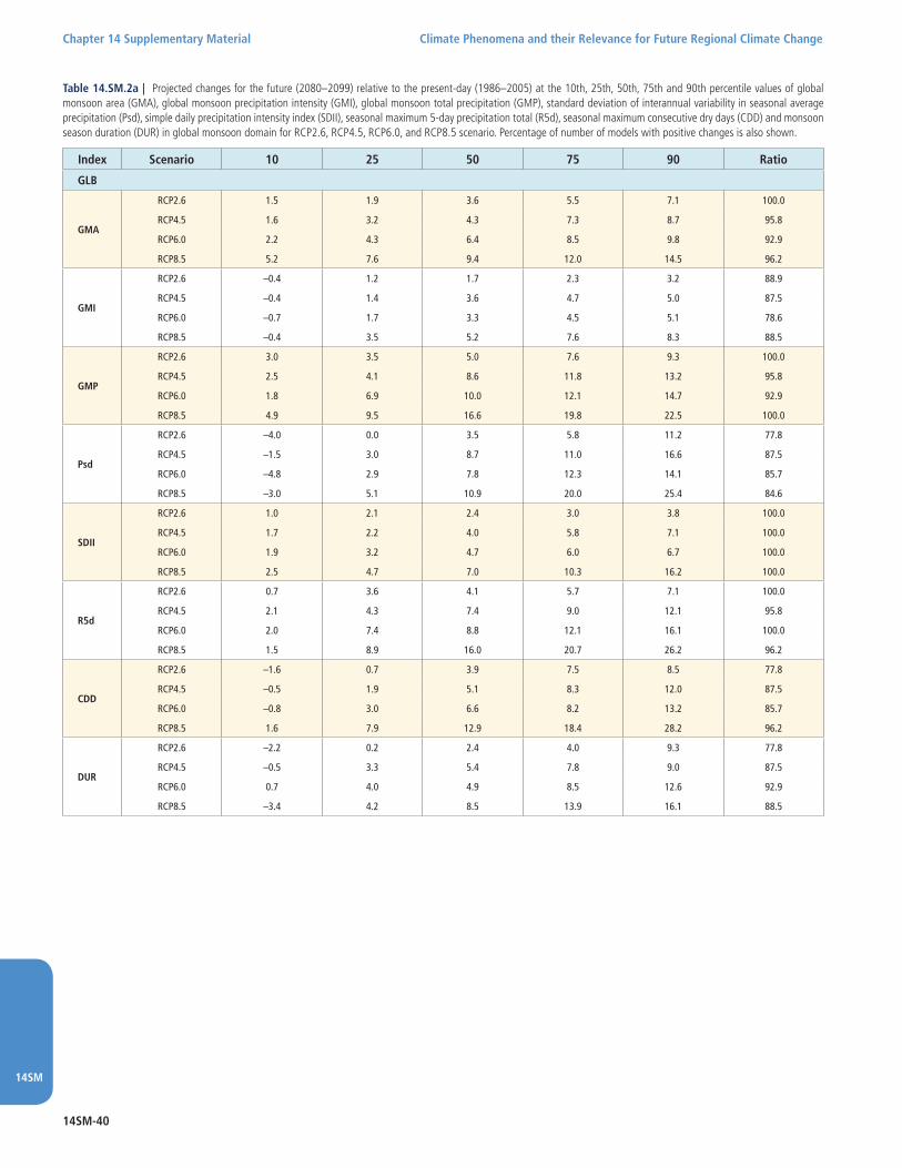
14SM-40
Chapter 14 Supplementary Material Climate Phenomena and their Relevance for Future Regional Climate Change
14SM
Table 14.SM.2a | Projected changes for the future (2080–2099) relative to the present-day (1986–2005) at the 10th, 25th, 50th, 75th and 90th percentile values of global monsoon area (GMA), global monsoon precipitation intensity (GMI), global monsoon total precipitation (GMP), standard deviation of interannual variability in seasonal average precipitation (Psd), simple daily precipitation intensity index (SDII), seasonal maximum 5-day precipitation total (R5d), seasonal maximum consecutive dry days (CDD) and monsoon season duration (DUR) in global monsoon domain for RCP2.6, RCP4.5, RCP6.0, and RCP8.5 scenario. Percentage of number of models with positive changes is also shown.
Index Scenario 10 25 50 75 90 Ratio
GLB
GMA
RCP2.6 1.5 1.9 3.6 5.5 7.1 100.0
RCP4.5 1.6 3.2 4.3 7.3 8.7 95.8
RCP6.0 2.2 4.3 6.4 8.5 9.8 92.9
RCP8.5 5.2 7.6 9.4 12.0 14.5 96.2
GMI
RCP2.6 –0.4 1.2 1.7 2.3 3.2 88.9
RCP4.5 –0.4 1.4 3.6 4.7 5.0 87.5
RCP6.0 –0.7 1.7 3.3 4.5 5.1 78.6
RCP8.5 –0.4 3.5 5.2 7.6 8.3 88.5
GMP
RCP2.6 3.0 3.5 5.0 7.6 9.3 100.0
RCP4.5 2.5 4.1 8.6 11.8 13.2 95.8
RCP6.0 1.8 6.9 10.0 12.1 14.7 92.9
RCP8.5 4.9 9.5 16.6 19.8 22.5 100.0
Psd
RCP2.6 –4.0 0.0 3.5 5.8 11.2 77.8
RCP4.5 –1.5 3.0 8.7 11.0 16.6 87.5
RCP6.0 –4.8 2.9 7.8 12.3 14.1 85.7
RCP8.5 –3.0 5.1 10.9 20.0 25.4 84.6
SDII
RCP2.6 1.0 2.1 2.4 3.0 3.8 100.0
RCP4.5 1.7 2.2 4.0 5.8 7.1 100.0
RCP6.0 1.9 3.2 4.7 6.0 6.7 100.0
RCP8.5 2.5 4.7 7.0 10.3 16.2 100.0
R5d
RCP2.6 0.7 3.6 4.1 5.7 7.1 100.0
RCP4.5 2.1 4.3 7.4 9.0 12.1 95.8
RCP6.0 2.0 7.4 8.8 12.1 16.1 100.0
RCP8.5 1.5 8.9 16.0 20.7 26.2 96.2
CDD
RCP2.6 –1.6 0.7 3.9 7.5 8.5 77.8
RCP4.5 –0.5 1.9 5.1 8.3 12.0 87.5
RCP6.0 –0.8 3.0 6.6 8.2 13.2 85.7
RCP8.5 1.6 7.9 12.9 18.4 28.2 96.2
DUR
RCP2.6 –2.2 0.2 2.4 4.0 9.3 77.8
RCP4.5 –0.5 3.3 5.4 7.8 9.0 87.5
RCP6.0 0.7 4.0 4.9 8.5 12.6 92.9
RCP8.5 –3.4 4.2 8.5 13.9 16.1 88.5

14SM-41
Climate Phenomena and their Relevance for Future Regional Climate Change Chapter 14 Supplementary Material
14SM
Table 14.SM.2b | Projected changes for the future (2080–2099) relative to the present–day (1986–2005) at the 10th, 25th, 50th, 75th and 90th percentile values of global mon-soon area (GMA), global monsoon precipitation intensity (GMI), global monsoon total precipitation (GMP), standard deviation of interannual variability in seasonal average precipi-tation (Psd), simple daily precipitation intensity index (SDII), seasonal maximum 5-day precipitation total (R5d), seasonal maximum consecutive dry days (CDD) and monsoon season duration (DUR) in each regional land monsoon domain for RCP2.6, RCP4.5, RCP6.0, and RCP8.5 scenario. Percentage of number of models with positive changes is also shown.
Index Scenario 10 25 50 75 90 Ratio
EAS
Pav
RCP2.6 –0.5 0.8 1.6 5.0 8.4 88.9
RCP4.5 1.3 2.7 5.7 9.0 9.8 91.7
RCP6.0 1.3 2.5 5.3 8.6 12.1 100.0
RCP8.5 2.6 4.1 7.8 12.5 17.0 92.3
Psd
RCP2.6 –10.6 –2.3 6.5 10.3 18.2 72.2
RCP4.5 3.2 6.2 12.1 14.2 25.4 91.7
RCP6.0 2.4 8.7 9.9 23.2 29.0 100.0
RCP8.5 10.9 17.7 25.4 30.2 32.8 96.2
SDII
RCP2.6 1.9 3.0 4.0 4.8 6.4 94.4
RCP4.5 2.9 6.0 7.8 9.1 12.3 95.8
RCP6.0 5.0 6.7 8.4 10.6 11.0 100.0
RCP8.5 8.3 12.6 14.2 17.1 20.8 96.2
R5d
RCP2.6 –1.0 2.3 4.0 8.3 10.5 88.9
RCP4.5 4.1 5.6 11.0 13.4 18.8 95.8
RCP6.0 7.5 9.6 10.4 16.9 20.9 100.0
RCP8.5 9.0 15.4 19.5 26.0 32.7 96.2
CDD
RCP2.6 –5.2 –3.3 1.1 6.8 14.5 61.1
RCP4.5 –6.8 –3.0 2.8 9.3 13.5 58.3
RCP6.0 –3.4 –1.9 –0.1 13.0 15.9 42.9
RCP8.5 –4.8 0.0 6.0 18.6 23.0 73.1
ONS
RCP2.6 –18 –10 –5 2 3 33.3
RCP4.5 –22 –15 –8 –2 0 8.3
RCP6.0 –17 –12 –6 3 8 28.6
RCP8.5 –30 –21 –11 –5 4 15.4
RET
RCP2.6 –22 0 3 13 20 66.7
RCP4.5 –3 2 8 12 38 79.2
RCP6.0 0 3 5 11 41 78.6
RCP8.5 –1 4 10 15 41 84.6
DUR
RCP2.6 –14 0 7 18 37 72.2
RCP4.5 –3 8 15 31 47 83.3
RCP6.0 –12 1 6 39 53 78.6
RCP8.5 4 7 20 42 54 92.3
SAS
Pav
RCP2.6 –0.4 1.9 4.5 6.7 7.8 88.9
RCP4.5 4.8 6.5 7.5 10.6 12.4 100.0
RCP6.0 4.3 6.2 8.2 10.1 10.8 100.0
RCP8.5 6.6 10.2 13.0 16.3 17.7 100.0
Psd
RCP2.6 –5.2 4.4 6.2 11.8 16.3 88.9
RCP4.5 1.5 6.9 13.9 20.3 25.4 95.8
RCP6.0 6.4 16.9 17.9 20.4 22.6 100.0
RCP8.5 7.8 10.9 25.5 32.0 49.1 100.0
SDII
RCP2.6 2.1 2.8 3.8 5.2 9.1 100.0
RCP4.5 5.2 6.2 7.2 10.1 13.5 100.0
RCP6.0 6.1 7.2 7.8 9.7 11.9 100.0
RCP8.5 8.8 10.8 15.1 17.5 23.1 100.0
(continued on next page)

14SM-42
Chapter 14 Supplementary Material Climate Phenomena and their Relevance for Future Regional Climate Change
14SM
Index Scenario 10 25 50 75 90 Ratio
R5d
RCP2.6 2.2 5.3 5.8 9.3 15.3 100.0
RCP4.5 5.1 9.8 12.4 16.2 21.2 100.0
RCP6.0 10.1 11.1 15.4 20.2 24.2 100.0
RCP8.5 11.7 18.3 22.4 38.0 47.5 96.2
CDD
RCP2.6 –7.2 –1.2 1.9 3.2 6.8 72.2
RCP4.5 –7.9 –5.0 –0.4 5.5 8.9 50.0
RCP6.0 –7.9 –5.4 –1.3 9.4 16.7 50.0
RCP8.5 –11.6 –4.9 6.7 11.7 17.1 69.2
ONS
RCP2.6 –7 –2 –1 2 3 33.3
RCP4.5 –6 –5 –3 0 1 16.7
RCP6.0 –7 –5 –2 2 5 42.9
RCP8.5 –11 –9 –5 –1 1 11.5
RET
RCP2.6 –2 1 2 6 10 77.8
RCP4.5 1 3 5 8 9 91.7
RCP6.0 2 3 4 10 13 92.9
RCP8.5 2 6 8 12 17 96.2
DUR
RCP2.6 –6 –2 4 7 15 72.2
RCP4.5 2 4 7 13 15 91.7
RCP6.0 –2 4 7 11 19 78.6
RCP8.5 4 8 13 19 24 96.2
AUSMC
Pav
RCP2.6 –8.1 –3.6 –1.5 2.1 4.0 44.4
RCP4.5 –8.7 0.3 3.2 7.1 8.7 83.3
RCP6.0 –4.2 –0.3 3.6 10.2 10.5 64.3
RCP8.5 –14.4 0.1 7.3 14.9 19.1 76.9
Psd
RCP2.6 –10.1 –0.1 3.2 11.1 20.9 72.2
RCP4.5 –1.2 1.0 6.8 12.6 28.2 83.3
RCP6.0 –2.6 –1.7 7.4 17.3 26.6 71.4
RCP8.5 –12.5 5.0 11.0 20.9 40.7 80.8
SDII
RCP2.6 –2.6 0.1 1.4 3.9 5.6 77.8
RCP4.5 –1.5 1.1 4.3 8.3 11.5 83.3
RCP6.0 –0.7 2.2 4.7 6.8 12.5 85.7
RCP8.5 –4.1 2.5 7.2 13.9 24.6 84.6
R5d
RCP2.6 –2.8 1.5 4.6 7.2 9.2 77.8
RCP4.5 –0.9 2.1 8.0 12.5 17.2 87.5
RCP6.0 1.2 1.9 9.8 15.7 27.7 92.9
RCP8.5 –3.8 3.5 15.0 26.7 36.5 88.5
CDD
RCP2.6 –1.7 –0.2 6.3 12.4 13.6 72.2
RCP4.5 –4.1 –0.6 4.1 12.5 21.5 75.0
RCP6.0 –8.0 –4.4 3.2 14.6 17.7 71.4
RCP8.5 –10.7 –2.4 6.8 25.8 36.8 69.2
ONS
RCP2.6 –19 –6 –2 6 21 38.9
RCP4.5 –12 –6 –5 4 11 37.5
RCP6.0 –13 –7 –4 5 9 28.6
RCP8.5 –18 –12 –6 8 13 36.0
RET
RCP2.6 –12 –2 5 10 15 55.6
RCP4.5 –5 –2 4 15 20 70.8
RCP6.0 2 3 6 11 17 92.9
RCP8.5 –8 1 8 13 27 76.0
Table 14.SM.2b (continued)
(continued on next page)

14SM-43
Climate Phenomena and their Relevance for Future Regional Climate Change Chapter 14 Supplementary Material
14SM
Table 14.SM.2b (continued)
(continued on next page)
Index Scenario 10 25 50 75 90 Ratio
DUR
RCP2.6 –16 –13 4 15 25 66.7
RCP4.5 –6 –2 7 14 21 75.0
RCP6.0 –4 1 5 18 26 78.6
RCP8.5 –21 –3 16 24 38 72.0
NAMS
Pav
RCP2.6 –5.3 –3.2 –1.9 2.6 5.5 44.4
RCP4.5 –12.9 –5.8 –2.9 0.8 5.0 33.3
RCP6.0 –6.0 –3.4 –2.0 6.7 7.0 42.9
RCP8.5 –25.4 –11.8 –6.5 3.5 6.9 26.9
Psd
RCP2.6 –7.8 –0.1 2.9 9.9 13.3 72.2
RCP4.5 –15.5 –5.5 2.5 13.5 18.4 62.5
RCP6.0 –7.3 –3.4 0.4 15.2 21.6 57.1
RCP8.5 –14.8 –9.1 1.5 17.1 37.2 61.5
SDII
RCP2.6 –2.6 –0.5 1.4 3.2 4.7 72.2
RCP4.5 –8.2 –3.0 0.1 3.9 10.9 54.2
RCP6.0 –2.7 0.3 1.3 7.6 10.8 85.7
RCP8.5 –16.5 –7.2 –0.1 13.1 19.1 50.0
R5d
RCP2.6 –1.6 0.2 3.6 4.6 11.8 77.8
RCP4.5 –6.5 –1.5 2.5 9.9 15.1 70.8
RCP6.0 –2.0 1.9 6.2 15.8 21.1 78.6
RCP8.5 –14.6 –3.0 6.7 21.0 38.5 69.2
CDD
RCP2.6 –3.2 0.9 3.9 10.2 16.6 77.8
RCP4.5 5.6 7.6 10.9 18.3 26.5 95.8
RCP6.0 3.0 4.8 9.4 14.0 15.9 92.9
RCP8.5 12.0 17.4 23.1 37.1 70.9 100.0
ONS
RCP2.6 –6 –3 1 3 7 58.8
RCP4.5 –7 –4 1 5 8 54.5
RCP6.0 –11 –4 –3 0 2 23.1
RCP8.5 –9 –4 1 8 13 52.2
RET
RCP2.6 –27 –8 2 8 12 52.9
RCP4.5 –7 –3 5 10 11 63.6
RCP6.0 –14 –8 1 10 18 53.8
RCP8.5 –47 –20 –1 20 23 47.8
DUR
RCP2.6 –29 –2 0 12 17 47.1
RCP4.5 –13 –3 2 10 16 54.5
RCP6.0 –10 –3 5 13 18 69.2
RCP8.5 –54 –29 8 18 22 52.2
SAMS
Pav
RCP2.6 –4.1 –3.2 –0.3 2.2 4.2 44.4
RCP4.5 –3.3 –1.1 1.2 4.2 6.5 66.7
RCP6.0 –2.4 –1.4 1.7 4.2 7.4 64.3
RCP8.5 –7.7 –2.6 2.4 6.2 11.2 69.2
Psd
RCP2.6 –4.1 –2.4 3.6 12.5 27.7 61.1
RCP4.5 –5.6 0.6 9.5 19.5 23.9 79.2
RCP6.0 –8.8 –4.1 3.9 10.7 25.7 71.4
RCP8.5 –9.2 2.5 16.8 27.1 46.0 84.6

14SM-44
Chapter 14 Supplementary Material Climate Phenomena and their Relevance for Future Regional Climate Change
14SM
Index Scenario 10 25 50 75 90 Ratio
SDII
RCP2.6 –1.9 0.7 1.6 2.6 4.8 83.3
RCP4.5 –0.6 1.1 3.1 6.0 11.1 83.3
RCP6.0 0.0 1.8 4.1 5.7 7.8 85.7
RCP8.5 –0.9 4.4 7.2 10.9 18.9 84.6
R5d
RCP2.6 –2.5 2.3 3.6 4.9 6.6 83.3
RCP4.5 –0.7 3.7 7.9 10.4 13.6 83.3
RCP6.0 –0.2 5.4 7.2 11.5 18.9 85.7
RCP8.5 –2.8 7.6 17.5 20.4 30.7 84.6
CDD
RCP2.6 –3.5 3.0 5.9 13.7 29.2 88.9
RCP4.5 1.9 3.0 9.0 14.1 19.3 95.8
RCP6.0 1.2 4.3 6.2 13.0 18.3 92.9
RCP8.5 7.7 15.5 19.3 38.8 48.4 96.2
ONS
RCP2.6 –6 –4 1 5 8 55.6
RCP4.5 –7 –4 1 5 7 54.2
RCP6.0 –6 –2 3 5 12 64.3
RCP8.5 –7 –5 0 9 14 50.0
RET
RCP2.6 –4 –2 0 0 2 22.2
RCP4.5 –4 –2 0 2 5 50.0
RCP6.0 –4 –2 0 2 3 42.9
RCP8.5 –8 –2 1 5 6 57.7
DUR
RCP2.6 –8 –5 –2 2 5 38.9
RCP4.5 –9 –7 –1 5 8 41.7
RCP6.0 –12 –8 –3 4 7 35.7
RCP8.5 –17 –10 0 8 11 50.0
NAF
Pav
RCP2.6 –3.7 –2.1 –0.4 2.3 3.5 50.0
RCP4.5 –4.4 –1.4 2.2 3.3 7.9 66.7
RCP6.0 –3.4 –1.6 1.0 6.4 13.7 64.3
RCP8.5 –6.7 –4.3 3.0 7.9 11.0 61.5
Psd
RCP2.6 –2.6 –1.4 2.2 6.5 16.7 72.2
RCP4.5 –4.6 –2.8 3.2 8.4 20.4 66.7
RCP6.0 –5.1 –2.3 5.1 15.6 28.0 71.4
RCP8.5 0.8 4.2 9.9 20.7 44.0 92.3
SDII
RCP2.6 –1.6 0.0 1.5 2.9 6.3 72.2
RCP4.5 –1.6 –0.5 2.9 6.4 9.3 75.0
RCP6.0 –1.7 0.9 1.8 7.3 8.4 85.7
RCP8.5 –0.6 1.4 6.8 9.9 23.1 84.6
R5d
RCP2.6 –0.6 0.6 1.8 5.3 15.8 88.9
RCP4.5 –2.9 1.1 6.6 9.5 16.9 79.2
RCP6.0 1.8 4.9 7.3 9.0 11.8 92.9
RCP8.5 1.9 8.8 13.2 22.4 40.3 96.2
CDD
RCP2.6 –5.7 2.1 3.4 9.3 13.1 88.9
RCP4.5 –4.9 –2.7 1.9 13.7 24.4 58.3
RCP6.0 –7.9 –4.1 4.2 7.9 11.1 57.1
RCP8.5 –0.2 5.2 10.9 39.9 49.2 88.5
ONS
RCP2.6 –8 –1 4 8 19 58.8
RCP4.5 –16 –1 2 9 14 73.9
RCP6.0 –11 –3 3 6 14 69.2
RCP8.5 –10 –8 –1 6 16 48.0
Table 14.SM.2b (continued)
(continued on next page)

14SM-45
Climate Phenomena and their Relevance for Future Regional Climate Change Chapter 14 Supplementary Material
14SM
Table 14.SM.2b (continued)
Index Scenario 10 25 50 75 90 Ratio
RET
RCP2.6 –4 –1 2 4 8 64.7
RCP4.5 –4 1 4 6 8 78.3
RCP6.0 4 4 6 13 14 92.3
RCP8.5 –4 5 9 15 20 88.0
DUR
RCP2.6 –23 –7 –4 4 14 35.3
RCP4.5 –15 –8 –1 8 20 43.5
RCP6.0 –4 –2 4 11 24 61.5
RCP8.5 –8 0 6 19 25 72.0
SAF
Pav
RCP2.6 –6.0 –3.4 –0.9 1.7 2.9 38.9
RCP4.5 –4.3 –1.6 2.1 3.4 4.1 62.5
RCP6.0 –4.2 –2.2 1.9 3.5 5.2 64.3
RCP8.5 –5.0 –1.2 2.6 5.4 7.0 69.2
Psd
RCP2.6 –6.9 –4.6 1.7 5.7 10.8 66.7
RCP4.5 –6.8 1.2 6.6 12.3 21.7 79.2
RCP6.0 –9.7 –0.7 0.6 16.0 24.7 57.1
RCP8.5 –1.9 6.0 14.3 24.7 33.0 84.6
SDII
RCP2.6 –1.9 0.9 1.7 2.5 3.6 83.3
RCP4.5 0.7 2.4 3.5 6.8 9.2 91.7
RCP6.0 –3.4 3.3 4.1 6.0 8.1 85.7
RCP8.5 4.1 5.5 7.5 12.2 21.3 92.3
R5d
RCP2.6 –3.8 0.6 2.4 4.6 6.8 83.3
RCP4.5 2.3 3.3 6.6 9.8 12.2 91.7
RCP6.0 –6.7 8.1 9.2 10.6 16.9 85.7
RCP8.5 5.7 10.2 16.7 19.8 24.0 92.3
CDD
RCP2.6 –3.6 0.5 6.6 13.7 16.0 77.8
RCP4.5 –1.5 2.5 9.2 15.8 18.4 87.5
RCP6.0 0.1 1.3 9.2 19.3 22.1 92.9
RCP8.5 7.0 12.8 20.3 32.0 38.7 96.2
ONS
RCP2.6 –11 –1 2 5 8 66.7
RCP4.5 –3 –1 2 4 5 70.8
RCP6.0 –2 1 2 7 10 78.6
RCP8.5 –2 1 5 10 14 80.8
RET
RCP2.6 –6 –3 –1 3 5 33.3
RCP4.5 –4 –2 0 4 9 50.0
RCP6.0 –5 1 1 9 12 78.6
RCP8.5 –2 3 6 9 14 80.8
DUR
RCP2.6 –14 –6 –3 2 8 33.3
RCP4.5 –7 –6 –1 6 9 45.8
RCP6.0 –14 –5 0 6 8 50.0
RCP8.5 –12 –5 –1 8 18 50.0

14SM-46
Chapter 14 Supplementary Material Climate Phenomena and their Relevance for Future Regional Climate Change
14SM
El Niño A B C D E F G H I
1950–1951 EP
1957–1958 EP EP EP
1963–1964 CP EP EP CP
1965–1966 EP EP M EP
1968–1969 CP CP CP CP CP
1969–1970 EP EP CP EP
1972–1973 EP EP EP M EP
1976–1977 EP EP EP M
1977–1978 CP CP CP CP CP CP
1979–1980 CP EP EP
1982–1983 EP EP EP EP M EP EP EP
1986–1987 EP EP M M CP EP EP
1987–1988 CP EP EP EP M M CP
1990–1991 CP CP CP CP CP CP
1991–1992 CP EP CP EP M M EP EP EP
1992–1993 CP CP CP
1994–1995 CP CP CP CP CP M CP CP CP
1997–1998 EP EP EP EP EP EP EP EP
2001–2002 CP
2002–2003 CP EP CP CP CP CP CP CP
2003–2004 EP
2004–2005 CP CP CP CP CP CP CP
2006–2007 EP EP EP CP CP
2009–2010 CP CP CP
Table 14.SM.3 | Lists of years for Eastern Pacific and Central Pacific El Niño events. A: Types based on Empirical Orthogonal Function (EOF) by (Ashok et al., 2007), B: Types based on the relative amplitude between NINO3 and NINO4 sea surface temperature (SST) index by (Yeh et al., 2009), C: similar to Yeh et al. (2009) but 1982–2010 climatology by Lee and McPhaden (2010), D: As in C but 1948-2006 climatology by Li et al. (2011b), E: similar to B but including ‘Mixed type, M’ by Kug et al. (2009), F: Types based on subsurface temperature by Yu et al. (2011), G: Types based on sea surface salinity for 1977–2008 by Singh et al. (2011), H: Modified Ashok et al. (2007) by Li et al. (2010a), I: Similar to Yeh et al. (2009) but 1950–2008 climatology by Hu et al. (2012). CP indicates ‘Central Pacific El Niño’, ‘date line El Niño’, or ‘El Niño-Modoki’ events; EP indicates ‘Eastern Pacific El Niño’ or ‘conventional El Niño’; M indicates the mixed type that belongs to neither EP nor CP type. Each paper uses different terminology but here EP, CP and M instead of various names.

14SM-47
Climate Phenomena and their Relevance for Future Regional Climate Change Chapter 14 Supplementary Material
14SM
Tabl
e 14
.SM
.4a
| Pr
ojec
ted
chan
ge in
freq
uenc
y of t
ropi
cal s
torm
s in
war
m cl
imat
e ru
ns re
lativ
e to
cont
rol r
un in
per
cent
. Red
and
blu
e nu
mbe
rs/te
xt d
enot
e pr
ojec
ted
incr
ease
s and
dec
reas
es, r
espe
ctiv
ely.
Bold
text
den
otes
whe
re a
stat
isti-
cal s
igni
fican
ce te
st w
as re
porte
d th
at sh
owed
sign
ifica
nce.
The
frequ
ency
pro
ject
ions
from
Em
anue
l et a
l. (20
08) h
ave
been
com
pute
d sli
ghtly
diff
eren
tly fr
om th
ose
show
n in
Fig
ure
8 of
the
orig
inal
pap
er in
ord
er to
facil
itate
inte
rcom
paris
on
with
pro
ject
ion
resu
lts fr
om o
ther
stu
dies
.
Trop
ical
Sto
rm F
requ
ency
Pro
ject
ions
(%)
Refe
renc
eM
odel
/typ
eRe
solu
tion
:hi
gh t
o lo
wEx
peri
men
tBa
sin
Glo
bal
NH
SHN
Atl.
NW
Pac
.N
E Pa
c.N
Ind.
S. In
d.SW
Pac
.
(Sug
i et a
l., 2
002)
JM
A tim
e sl
ice
T106
L21
(~12
0 km
)10
yr
1 ×
CO2,
2 ×
CO2
–34
–28
–39
+61
–66
–67
+9
–57
–31
(McD
onal
d et
al.,
200
5)
HadA
M3
time
slic
eN
144
L30
(~10
0 km
)15
yr I
S95a
1979
–199
420
82–2
097
–6–3
–10
–30
–30
+80
+42
+10
–18
(Has
egaw
a an
d Em
ori,
2005
) CC
SR/N
IES/
FRCG
C tim
e sl
ice
T106
L56
(~12
0 km
)5 ×
20 y
r at 1
× C
O2
7 ×
20 y
r at 2
× C
O2
–4
(Yos
him
ura
et a
l., 2
006)
JM
A tim
e sl
ice
T106
L21
(~12
0 km
)10
yr 1
× C
O2,
2 ×
CO2
–15
(Oou
chi e
t al.,
200
6)M
RI/JM
A tim
e sl
ice
TL95
9 L6
0(~
20 k
m)
10 y
r A1B
1982
–199
320
80–2
099
–30
–28
–32
+34
–38
–34
–52
–28
–43
(Cha
uvin
et a
l., 2
006)
AR
PEG
E Cl
imat
tim
e sl
ice
~50
km
Do
wns
cale
CN
RM B
2Do
wns
cale
Had
ley
A2+
18 –25
(Sto
was
ser e
t al.,
200
7)IP
RC R
egio
nal
Dow
nsca
le N
CAR
CCSM
2, 6
× C
O2
+19
(Ben
gtss
on e
t al.,
200
7)
ECHA
M5
time
slic
eT2
13
(~60
km
)20
71–2
100,
A1B
–13
–8–2
0+
4–2
6
(Ben
gtss
on e
t al.,
200
7)
ECHA
M5
time
slic
eT3
19(~
40 k
m)
2071
–210
0, A
1B–1
9–1
3–2
8+
7–5
1
(Em
anue
l et a
l., 2
008)
Stat
istic
al-
dete
rmin
istic
--
-Do
wns
cale
7 C
MIP
3 m
ods.:
A1B
, 218
0–22
00Av
erag
e ov
er s
even
mod
els
–7+
2–1
3+
4+
6–5
–7–1
2–1
5
(Knu
tson
et a
l., 2
008)
GFD
L Ze
tac
regi
onal
18
km
Dow
nsca
le C
MIP
3 en
s. A1
B, 2
080–
2100
–27
(Knu
tson
et a
l., 2
013)
GFD
L Ze
tac
regi
onal
18 k
mDo
wns
cale
(yr 2
081–
2100
) CM
IP3
ens.
A1B
CMIP
5 en
s Rc
p45
Gfd
l CM
2.1
A1B
MPI
A1B
HadC
M3
A1B
MRI
A1B
Gfd
l CM
2.0
A1B
HadG
EM1
A1B
MIR
OC
hi A
1BCC
MS3
A1B
ING
V A1
BM
IRO
C m
ed A
1B
–27
–23
–9 –38
–52
–25
+8
–62
–33
–28
–22
–43
(Les
lie e
t al.,
200
7)O
U-C
GCM
with
hi
gh-r
es. w
indo
wU
p to
50
km20
00 to
205
0 co
ntro
l an
d IS
92a
(6 m
embe
rs)
~0
(con
tinue
d on
nex
t pag
e)

14SM-48
Chapter 14 Supplementary Material Climate Phenomena and their Relevance for Future Regional Climate Change
14SM
Trop
ical
Sto
rm F
requ
ency
Pro
ject
ions
(%)
Refe
renc
eM
odel
/typ
eRe
solu
tion
:hi
gh t
o lo
wEx
peri
men
tBa
sin
Glo
bal
NH
SHN
Atl.
NW
Pac
.N
E Pa
c.N
Ind.
S. In
d.SW
Pac
.
(Gua
ldi e
t al.,
200
8)
SIN
TEX-
G
coup
led
mod
elT1
06(~
120
km)
30 y
r 1 ×
CO
2, 2 ×
CO2,
4 ×
CO2
–16
(2×
) –
44 (4
×)
–14
–20
–3–1
3–1
4–2
2
(Sem
mle
r et a
l., 2
008)
Ross
by C
entr
e re
gion
al m
odel
28 k
m16
yr c
ontr
ol a
nd
A2, 2
085–
2100
–13
(Zha
o et
al.,
200
9)
GFD
L HI
RAM
tim
e sl
ice
50 k
mDo
wns
cale
A1B
:CM
IP3
n =
18 e
ns.
GFD
L CM
2.1
HadC
M3
ECHA
M5
–20
–20
–11
–20
–14
–14
+5
–17
–32
–33
–42
–27
–39
–5 –62
–1
–29
–5 –12
–52
+15 –23
+61
+35
–2 –43
–2 –25
–30
–33
–41
–13
–32
–31
–42
–48
(Sug
i et a
l., 2
009)
JMA/
MRI
glo
bal
AGCM
tim
e sl
ice
20 k
m20
km
20 k
m20
km
60 k
m60
km
60 k
m60
km
Dow
nsca
le A
1B:
MRI
CG
CM2.
3M
RI C
GCM
2.3
MIR
OC-
HCM
IP3
n =
18
ens.
MRI
CG
CM2.
3M
IRO
C-H
CMIP
3 n
= 1
8 en
s.CS
IRO
–29
–25
–27
–20
–20
–6 –21
–22
–31
–25
–15
–21
–21 0 –19
–29
–27
–25
–42
–19
–17
–16
–25
–11
+22
+23 –18
+5
+58 +6
+4
–37
–36
–29
+28 –26
–36
+64 –14
+13
–39
–30
–50
–25
–31
–42
–33
–49
–39
–29
+32 –15
–12
+79 +33 –7
–28
–25
–24
–5 –22
+10 –18
–22
–22
–27
–90
–42
–8 –69
–36
+10
(Mur
akam
i et a
l., 2
012)
JMA/
MRI
glo
bal
AGCM
tim
e sl
ice
V3.1
20
kmV3
.2 2
0 km
V3.1
60
kmV3
.2 6
0 km
Dow
nsca
le C
MIP
3 m
ulti-
mod
el e
ns. A
1B c
hang
e (2
075–
2099
min
us c
ontr
ol)
–23
–15
–23
–24
–20
–14
–23
–23
–25
–18
–24
–25
+8
–29
–2 –39
–27
–23
–20
–28
–24
+1
–32
–10
–14
–2 +21 –14
–10
–23
–15
–24
–45
–15
–39
–27
(Mur
akam
i et a
l., 2
011)
JMA/
MRI
glo
bal
AGCM
tim
e sl
ice
V3.2
60
kmDo
wns
cale
A1B
:YS
, CM
IP3
ens.
YS, C
lust
er 1
YS, C
lust
er 2
YS, C
lust
er 3
KF, C
MIP
3 en
s.KF
, Clu
ster
1KF
, Clu
ster
2KF
, Clu
ster
3AS
, CM
IP3
ens.
AS, C
lust
er 1
AS, C
lust
er 2
AS, C
lust
er 3
–27
–25
–28
–14
–20
–20
–21
–14
–20
–22
–13
–14
–27
–25
–30
–3 –24
–27
–28
–12
–11
–22
–11 0
–27
–27
–26
–35
–16
–10
–12
–15
–33
–24
–17
–32
–44
–24
–23
–31
–39
–40
–21
–53
+1
–27
+28 –24
–33
–32
–42
–2 –28
–33
–44
–8 –19
–19
–32
+8
–11
–30
–9 +6 –3 –15
+5
+17 –22
–42
+24
+15
–16
+19 –21
+1
–42
–28
–50
–48
+1
–20
–5 –15
–29
–24
–20
–46
–24
–20
–10
–26
–31
–25
–2 –48
–31
–37
–42
–25
–11
–6 –24
–6 –43
–27
–44
–11
(Vill
arin
i et a
l., 2
011)
Stat
istic
al
dow
nsca
le o
f CM
IP3
mod
els
---
24 C
MIP
3 m
odel
mea
n an
d ±
1 σ
rang
e; A
1B s
cena
rio,
21st
cen
tury
tren
d
Basi
n:–1
0 ±
29%
U
S la
nd:
–3 ±
26
(Em
anue
l et a
l., 2
010)
Stat
istic
al-
dete
rmin
istic
--
Tim
e sl
ice
usin
g CM
IP3
mod
el m
ean
SST
chan
ge,
1990
–209
0, N
ICAM
mod
el
14 k
m
+45
(glo
bal
but J
une
to
Oct
ober
onl
y)
(Yam
ada
et a
l., 2
010)
NIC
AM14
km
Tim
e sl
ice
usin
g CM
IP3
mod
el m
ean
SST
chan
ge, 1
990–
2090
–35
(glo
bal
but J
une
to
Oct
ober
onl
y)
–80
00
–77
Tabl
e 14
.SM
.4a
(con
tinue
d)
(con
tinue
d on
nex
t pag
e)

14SM-49
Climate Phenomena and their Relevance for Future Regional Climate Change Chapter 14 Supplementary Material
14SM
Tabl
e 14
.SM
.4a
(con
tinue
d)
Trop
ical
Sto
rm F
requ
ency
Pro
ject
ions
(%)
Refe
renc
eM
odel
/typ
eRe
solu
tion
:hi
gh t
o lo
wEx
peri
men
tBa
sin
Glo
bal
NH
SHN
Atl.
NW
Pac
.N
E Pa
c.N
Ind.
S. In
d.SW
Pac
.
(Lav
ende
r and
Wal
sh, 2
011)
CSIR
O C
CAM
re
gion
al m
odel
ne
sted
in a
sui
te
of G
CMs
15 k
mA2
199
0, 2
090
GFD
L CM
2.1
MPI
ECH
AM5
CSIR
O M
k3.5
–38
–33
–27
(Li e
t al.,
201
0d)
ECHA
M5
time
slic
e40
km
A1B
chan
ge(2
080–
2009
)–3
1+
65
(Yok
oi a
nd Ta
kaya
bu, 2
009)
CMIP
3 en
sem
ble
Vario
usA1
B (2
081–
2100
)–1
(Mur
akam
i et a
l., 2
013)
JMA/
MRI
glo
bal
AGCM
tim
e sl
ice
V3.2
60
kmAs
in M
urak
ami e
t al.
(201
1), b
ut u
sing
diff
eren
t cr
iteria
for T
C de
tect
ion
–2
(Vill
arin
i and
Vec
chi,
2012
)St
atis
tical
do
wns
cale
of
CMIP
5 m
odel
s
--17
CM
IP5
mod
els
Mea
n an
d (m
in/m
ax ra
nge)
RCP2
.6
RCP4
.5
RCP8
.5(la
te 2
1st c
entu
ry)
4 (–
17,3
2)4
(–30
,57)
2(–
49,4
5)

14SM-50
Chapter 14 Supplementary Material Climate Phenomena and their Relevance for Future Regional Climate Change
14SM
Tabl
e 14
.SM
.4b
| Pro
ject
ed ch
ange
in fr
eque
ncy o
f int
ense
trop
ical c
yclo
nes (
i.e.,
mor
e in
tens
e th
an tr
opica
l sto
rms)
in w
arm
clim
ate
runs
rela
tive
to co
ntro
l run
in p
erce
nt. T
he ro
ws o
f rep
orte
d re
sults
are
ord
ered
from
top
to b
otto
m g
ener
ally
in o
rder
of d
ecre
asin
g m
odel
hor
izont
al re
solu
tion.
Red
and
blu
e nu
mbe
rs/te
xt d
enot
e pr
ojec
ted
incr
ease
s an
d de
crea
ses,
resp
ectiv
ely.
Bold
text
den
otes
whe
re a
sta
tistic
al s
igni
fican
ce te
st w
as re
porte
d th
at s
how
ed s
igni
fican
ce.
Inte
nse
Trop
ical
Cyc
lone
Fre
quen
cy P
roje
ctio
ns (%
)
Refe
renc
eM
odel
/typ
eRe
solu
tion
:hi
gh t
o lo
wEx
peri
men
tBa
sin
Glo
bal
NH
SHN
Atl.
NW
Pac
.N
E Pa
c.N
Ind.
S. In
d.SW
Pac
.
(Ben
der e
t al.,
201
0)G
FDL
Hurr
ican
e m
odel
,w
ith o
cean
cou
plin
g9
kmDo
wns
cale
TCs
from
ref 2
218
-mod
ens
embl
e:(ra
nge
over
4 in
div.
mod
els)
cat 4
–5fre
q:+
100%
(–66
to +
138%
)
(Knu
tson
et a
l., 2
013)
GFD
L Hu
rric
ane
mod
el,
with
oce
an c
oupl
ing
9 km
Dow
nsca
le T
Cs(2
081–
2100
)CM
IP3
ens.
A1B
CMIP
5 en
s RC
P45
Gfd
l CM
2.1
A1B
MPI
A1B
HadC
M3
A1B
MRI
A1B
Gfd
l CM
2.0
A1B
HadG
EM1
A1B
MIR
OC
hi A
1BCC
MS3
A1B
ING
V A1
BM
IRO
C m
ed A
1B
cat 4
–5fre
q:+
87%
+39
%+
116%
+21
%–5
3%+
110%
+21
1%–1
00%
–42%
+26
%+
47%
–32%
(Knu
tson
et a
l., 2
008)
G
FDL
Zeta
c re
gion
al
18 k
mDo
wns
cale
CM
IP3
ens.
A1B,
208
0–21
00+
140%
(12
vs 5
) #
w/V
sfc >
45
m s
–1
(Mur
akam
i et a
l., 2
013)
JMA/
MRI
glo
bal
AGCM
tim
e sl
ice
V3.2
20
kmDo
wns
cale
CM
IP3
mul
ti-m
odel
ens
. A1B
cha
nge
(207
5–20
99 m
inus
con
trol
)
# Ca
t 4–
5:
+4%
# Ca
t. 5:
+
56%
+9%
+60
%
–7%
+43
%
+15
%
+28
7%
–4%
+45
%
+17
9%
Incr
ease
from
0
+35
%
+10
0%
+45
%
+26
1%
–54%
–61%
(Oou
chi e
t al.,
200
6)M
RI/JM
Atim
e sl
ice
TL95
9 L6
0 (~
20 k
m)
10 y
r A1B
1982
–199
320
80–2
099
Sign
if.
Incr
ease
, # V
850
of 5
5–60
m s
–1
(Wal
sh e
t al.,
200
4)CS
IRO
DAR
LAM
re
gion
al m
odel
30 k
m3
× C
O2;
2061
–209
0 m
inus
196
1–19
90+
26%
P
< 9
70 m
b
(Ben
gtss
on e
t al.,
200
7)EC
HAM
5 tim
e sl
ice
T319
(~40
km
)20
71–2
100,
A1B
+42
%, #
>
50 m
s–1
(Zha
o an
d He
ld, 2
010)
GFD
L HI
RAM
tim
e sl
ice
with
sta
tistic
al
refin
emen
t of i
nten
sity
50 k
mDo
wns
cale
A1B
:CM
IP3
n =
7 e
ns.
GFD
L CM
2.0
GFD
L CM
2.1
HadC
M3
HadG
em1
ECHA
M5
MRI
_CG
CM2.
3M
IRO
C Hi
gh
cat 3
–5 h
urr %
–13
+9
+5
–28
–53
+24 0 –27
(con
tinue
d on
nex
t pag
e)
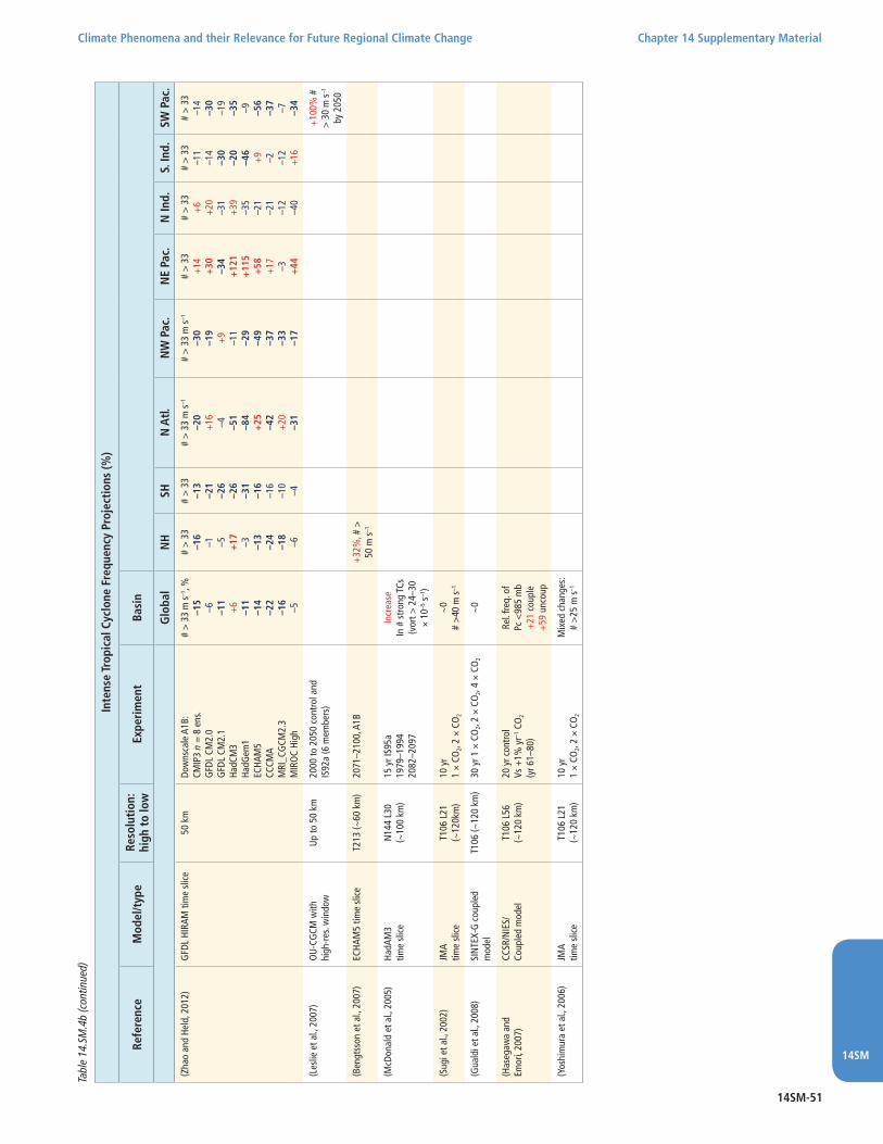
14SM-51
Climate Phenomena and their Relevance for Future Regional Climate Change Chapter 14 Supplementary Material
14SM
Tabl
e 14
.SM
.4b
(con
tinue
d)
Inte
nse
Trop
ical
Cyc
lone
Fre
quen
cy P
roje
ctio
ns (%
)
Refe
renc
eM
odel
/typ
eRe
solu
tion
:hi
gh t
o lo
wEx
peri
men
tBa
sin
Glo
bal
NH
SHN
Atl.
NW
Pac
.N
E Pa
c.N
Ind.
S. In
d.SW
Pac
.
(Zha
o an
d He
ld, 2
012)
GFD
L HI
RAM
tim
e sl
ice
50 k
mDo
wns
cale
A1B
:CM
IP3
n =
8 e
ns.
GFD
L CM
2.0
GFD
L CM
2.1
HadC
M3
HadG
em1
ECHA
M5
CCCM
AM
RI_C
GCM
2.3
MIR
OC
High
# >
33
m s
–1, %
–15
–6 –11
+6
–11
–14
–22
–16
–5
# >
33
–16
–1 –5 +17 –3 –13
–24
–18
–6
# >
33
–13
–21
–26
–26
–31
–16
–16
–10
–4
# >
33
m s
–1
–20
+16 –4 –51
–84
+25 –42
+20 –31
# >
33
m s
–1
–30
–19
+9
–11
–29
–49
–37
–33
–17
# >
33
+14
+30 –34
+12
1+
115
+58 +17 –3 +44
# >
33
+6
+20 –31
+39 –35
–21
–21
–12
–40
# >
33
–11
–14
–30
–20
–46
+9 –2 –12
+16
# >
33
–14
–30
–19
–35
–9 –56
–37
–7 –34
(Les
lie e
t al.,
200
7)
OU
-CG
CM w
ith
high
-res
. win
dow
Up
to 5
0 km
2000
to 2
050
cont
rol a
nd
IS92
a (6
mem
bers
)+
100%
#
> 3
0 m
s–1
by
205
0
(Ben
gtss
on e
t al.,
200
7)EC
HAM
5 tim
e sl
ice
T213
(~60
km
)20
71–2
100,
A1B
+32
%, #
>
50 m
s–1
(McD
onal
d et
al.,
200
5)Ha
dAM
3tim
e sl
ice
N14
4 L3
0 (~
100
km)
15 y
r IS9
5a19
79–1
994
2082
–209
7
Incr
ease
In #
str
ong
TCs
(vor
t > 2
4–30
×
10–5
s–1
)
(Sug
i et a
l., 2
002)
JM
Atim
e sl
ice
T106
L21
(~12
0km
)10
yr
1 ×
CO2,
2 ×
CO2
~0
# >
40 m
s–1
(Gua
ldi e
t al.,
200
8)
SIN
TEX-
G c
oupl
ed
mod
elT1
06 (~
120
km)
30 y
r 1 ×
CO
2, 2 ×
CO2,
4 ×
CO2
~0
(Has
egaw
a an
d Em
ori,
2007
) CC
SR/N
IES/
Co
uple
d m
odel
T1
06 L
56(~
120
km)
20 y
r con
trol
Vs +
1% y
r–1 C
O2
(yr 6
1–80
)
Rel.
freq.
of
Pc <
985
mb
+21
cou
ple
+59
unc
oup
(Yos
him
ura
et a
l., 2
006)
JMA
time
slic
eT1
06 L
21(~
120
km)
10 y
r 1 ×
CO2,
2 ×
CO2
Mix
ed c
hang
es:
# >
25 m
s–1
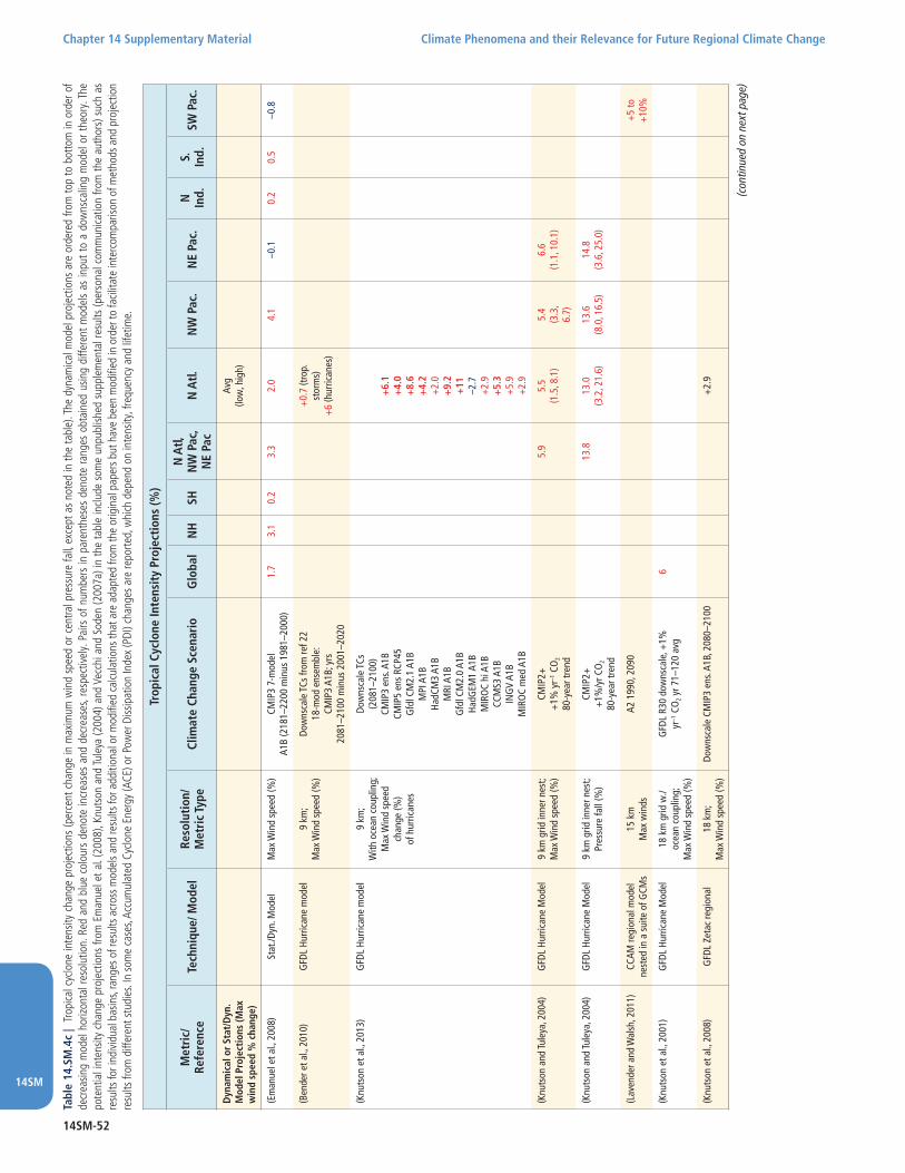
14SM-52
Chapter 14 Supplementary Material Climate Phenomena and their Relevance for Future Regional Climate Change
14SM
Tabl
e 14
.SM
.4c
| Tr
opica
l cyc
lone
inte
nsity
cha
nge
proj
ectio
ns (p
erce
nt c
hang
e in
max
imum
win
d sp
eed
or c
entra
l pre
ssur
e fa
ll, ex
cept
as
note
d in
the
tabl
e). T
he d
ynam
ical m
odel
pro
ject
ions
are
ord
ered
from
top
to b
otto
m in
ord
er o
f de
crea
sing
mod
el h
orizo
ntal
reso
lutio
n. R
ed a
nd b
lue
colo
urs
deno
te in
crea
ses
and
decr
ease
s, re
spec
tivel
y. Pa
irs o
f num
bers
in p
aren
thes
es d
enot
e ra
nges
obt
aine
d us
ing
diffe
rent
mod
els
as in
put t
o a
dow
nsca
ling
mod
el o
r the
ory.
The
pote
ntia
l int
ensit
y ch
ange
pro
ject
ions
from
Em
anue
l et a
l. (2
008)
, Knu
tson
and
Tule
ya (2
004)
and
Vec
chi a
nd S
oden
(200
7a) i
n th
e ta
ble
inclu
de s
ome
unpu
blish
ed s
uppl
emen
tal r
esul
ts (p
erso
nal c
omm
unica
tion
from
the
auth
ors)
suc
h as
re
sults
for i
ndiv
idua
l bas
ins,
rang
es o
f res
ults
acr
oss m
odel
s and
resu
lts fo
r add
ition
al o
r mod
ified
cal
cula
tions
that
are
ada
pted
from
the
orig
inal
pap
ers b
ut h
ave
been
mod
ified
in o
rder
to fa
cilita
te in
terc
ompa
rison
of m
etho
ds a
nd p
roje
ctio
n re
sults
from
diff
eren
t stu
dies
. In
som
e ca
ses,
Accu
mul
ated
Cyc
lone
Ene
rgy
(ACE
) or P
ower
Diss
ipat
ion
Inde
x (P
DI) c
hang
es a
re re
porte
d, w
hich
dep
end
on in
tens
ity, f
requ
ency
and
life
time.
Trop
ical
Cyc
lone
Inte
nsit
y Pr
ojec
tion
s (%
)
Met
ric/
Refe
renc
eTe
chni
que/
Mod
elRe
solu
tion
/M
etri
c Ty
peCl
imat
e Ch
ange
Sce
nari
oG
loba
lN
HSH
N A
tl,
NW
Pac
, N
E Pa
cN
Atl.
NW
Pac
.N
E Pa
c.N
In
d.S.
In
d.SW
Pac
.
Dyn
amic
al o
r St
at/D
yn.
Mod
el P
roje
ctio
ns (M
ax
win
d sp
eed
% c
hang
e)
Avg
(low
, hig
h)
(Em
anue
l et a
l., 2
008)
Stat
./Dyn
. Mod
elM
ax W
ind
spee
d (%
)CM
IP3
7-m
odel
A1B
(218
1–22
00 m
inus
198
1–20
00)
1.7
3.1
0.2
3.3
2.0
4.1
–0.1
0.
2 0.
5–0
.8
(Ben
der e
t al.,
201
0)
GFD
L Hu
rric
ane
mod
el9
km;
Max
Win
d sp
eed
(%)
Dow
nsca
le T
Cs fr
om re
f 22
18-m
od e
nsem
ble:
CMIP
3 A1
B; y
rs20
81–2
100
min
us 2
001–
2020
+0.
7 (tr
op.
stor
ms)
+6
(hur
rican
es)
(Knu
tson
et a
l., 2
013)
GFD
L Hu
rric
ane
mod
el
9 km
; W
ith o
cean
cou
plin
g;M
ax W
ind
spee
d ch
ange
(%)
of h
urric
anes
Dow
nsca
le T
Cs(2
081–
2100
)CM
IP3
ens.
A1B
CMIP
5 en
s RC
P45
Gfd
l CM
2.1
A1B
MPI
A1B
HadC
M3
A1B
MRI
A1B
Gfd
l CM
2.0
A1B
HadG
EM1
A1B
MIR
OC
hi A
1BCC
MS3
A1B
ING
V A1
BM
IRO
C m
ed A
1B
+6.
1+
4.0
+8.
6+
4.2
+2.
0+
9.2
+11
–2.7
+2.
9+
5.3
+5.
9+
2.9
(Knu
tson
and
Tule
ya, 2
004)
GFD
L Hu
rric
ane
Mod
el9
km g
rid in
ner n
est;
Max
Win
d sp
eed
(%)
CMIP
2+
+1%
yr–1
CO
2
80-y
ear t
rend
5.9
5.5
(1.5
, 8.1
)5.
4(3
.3,
6.7)
6.6
(1.1
, 10.
1)
(Knu
tson
and
Tule
ya, 2
004)
G
FDL
Hurr
ican
e M
odel
9 km
grid
inne
r nes
t; Pr
essu
re fa
ll (%
)CM
IP2+
+
1%/y
r CO
2
80-y
ear t
rend
13.8
13.0
(3.2
, 21.
6)13
.6(8
.0, 1
6.5)
14.8
(3.6
, 25.
0)
(Lav
ende
r and
Wal
sh, 2
011)
CCAM
regi
onal
mod
el
nest
ed in
a s
uite
of G
CMs
15 k
mM
ax w
inds
A2 1
990,
209
0+
5 to
+
10%
(Knu
tson
et a
l., 2
001)
GFD
L Hu
rric
ane
Mod
el18
km
grid
w./
ocea
n co
uplin
g;M
ax W
ind
spee
d (%
)
GFD
L R3
0 do
wns
cale
, +1%
yr
–1 C
O2 y
r 71–
120
avg
6
(Knu
tson
et a
l., 2
008)
GFD
L Ze
tac
regi
onal
18
km
;M
ax W
ind
spee
d (%
)Do
wns
cale
CM
IP3
ens.
A1B,
208
0–21
00+
2.9
(con
tinue
d on
nex
t pag
e)

14SM-53
Climate Phenomena and their Relevance for Future Regional Climate Change Chapter 14 Supplementary Material
14SM
Trop
ical
Cyc
lone
Inte
nsit
y Pr
ojec
tion
s (%
)
Met
ric/
Refe
renc
eTe
chni
que/
Mod
elRe
solu
tion
/M
etri
c Ty
peCl
imat
e Ch
ange
Sce
nari
oG
loba
lN
HSH
N A
tl,
NW
Pac
, N
E Pa
cN
Atl.
NW
Pac
.N
E Pa
c.N
In
d.S.
In
d.SW
Pac
.
(Knu
tson
et a
l., 2
013)
GFD
L Ze
tac
regi
onal
18
km
;M
ax W
ind
spee
d (%
)of
hur
rican
es
Dow
nsca
le T
Cs(2
081–
2100
)CM
IP3
ens.
A1B
CMIP
5 en
s RC
P45
Gfd
l CM
2.1
A1B
MPI
A1B
HadC
M3
A1B
MRI
A1B
Gfd
l CM
2.0
A1B
HadG
EM1
A1B
MIR
OC
hi A
1BCC
MS3
A1B
ING
V A1
BM
IRO
C m
ed A
1B
+2.
0+
2.2
+2.
8+
3.6
+0.
9+
4.0
+3.
6+
1.5
+2.
3+
3.8
+2.
0+
2.1
(Mur
akam
i et a
l., 2
013)
JMA/
MRI
glo
bal
AGCM
tim
e sl
ice
V3.1
20
kmV3
.2 2
0 km
;Av
g. m
ax w
inds
ove
r lif
etim
e of
all
TCs
Dow
nsca
le C
MIP
3 m
ulti-
mod
el e
ns. A
1B
chan
ge (2
075–
2099
min
us c
ontr
ol)
11 412 6
10 05 10
18 712 6
5 710 7
8 –10
(Oou
chi e
t al.,
200
6)M
RI/JM
ATi
me
slic
eTL
959
L60
(~20
km
) Avg
. life
time
max
win
dspe
ed
10 y
r A1B
1982
–199
320
80–2
099
10.7
8.5
14.1
11.2
4.2
0.6
–12.
817
.3–2
.0
(Oou
chi e
t al.,
200
6)M
RI/JM
Atim
e sl
ice
TL95
9 L6
0 (~
20
km) A
vg. a
nnua
l m
ax w
inds
10 y
r A1B
1982
–199
320
80–2
099
13.7
15.5
6.9
20.1
–2.0
–5.0
–16.
78.
2–2
2.5
(Sem
mle
r et a
l., 2
008)
Ross
by C
entr
e re
gion
al m
odel
28 k
m;
Max
win
ds16
-yea
r con
trol
and
A2,
208
5–21
00+
4
(Cha
uvin
et a
l., 2
006)
AR
PEG
E Cl
imat
time
slic
e~
50 k
m
Max
win
dsDo
wns
cale
- CN
RM B
2 - H
adle
y A2
~0
~0
(Sug
i et a
l., 2
002)
JM
Atim
e sl
ice
T106
L21
(~12
0 km
)M
ax w
inds
10 y
r1 ×
CO2,
2 ×
CO2
~0
(Gua
ldi e
t al.,
200
8)
SIN
TEX-
G c
oupl
ed m
odel
T106
(~12
0 km
); M
ax w
inds
30 y
r 1 ×
CO
2, 2 ×
CO2,
4 ×
CO2
~0
(Has
egaw
a an
d Em
ori,
2005
) CC
SR/N
IES/
FRCG
C tim
e sl
ice
T106
L56
(~12
0 km
)M
ax w
inds
5 ×
20 y
r at 1
× C
O2
7 ×
20 y
r at 2
× C
O2
Decr
ease
(Yos
him
ura
et a
l., 2
006)
JM
Atim
e sl
ice
T106
L21
(~12
0 km
)M
ax w
inds
10 y
r 1 ×
CO2,
2 ×
CO2
~0
(Has
egaw
a an
d Em
ori,
2007
)CC
SR/N
ICS/
FRC
Coup
led
GCM
T106
L56
(~12
0 km
) M
ax w
inds
20-y
ear c
ontr
olVs
+1%
yr–1
CO
2
(yr 6
1–80
)
~0
for
Pc <
98
5 m
b
Tabl
e 14
.SM
.4c
(con
tinue
d)
(con
tinue
d on
nex
t pag
e)

14SM-54
Chapter 14 Supplementary Material Climate Phenomena and their Relevance for Future Regional Climate Change
14SM
Tabl
e 14
.SM
.4c
(con
tinue
d)
Trop
ical
Cyc
lone
Inte
nsit
y Pr
ojec
tion
s (%
)
Met
ric/
Refe
renc
eTe
chni
que/
Mod
elRe
solu
tion
/M
etri
c Ty
peCl
imat
e Ch
ange
Sce
nari
oG
loba
lN
HSH
N A
tl,
NW
Pac
, N
E Pa
cN
Atl.
NW
Pac
.N
E Pa
c.N
In
d.S.
In
d.SW
Pa
c.
Pote
ntia
l Int
ensi
ty
Theo
ry P
roje
ctio
ns o
f In
tens
ity
(% C
hang
e)
Avg
(low
, hig
h)
(Vec
chi a
nd S
oden
, 200
7b)
Eman
uel P
I, re
vers
ible
w/ d
iss.
heat
ing
Max
Win
d sp
eed
(%)
CMIP
3 18
-mod
el A
1B
(100
-yea
r tre
nd)
2.6
2.7
2.4
2.1
0.05
(–8.
0, 4
.6)
2.9
(–3.
1, 1
2.6)
3.5
(–6.
4 16
.1)
4.4
(–3.
3,
16.0
)
3.7
(–7.
6,
17.1
)
0.99
(–8.
6,
8.6)
(Knu
tson
and
Tule
ya, 2
004)
Pote
ntia
l Int
ensi
ty
Eman
uel,
reve
rsib
le
Pres
sure
fall
(%)
CMIP
2+
+1%
yr–1
CO
2
80-y
ear t
rend
5.0
2.6
(–5.
6, 1
2.6)
7.0
(–1.
0, 1
9.6)
5.4
(–5.
0,
21.9
)
(Knu
tson
and
Tule
ya, 2
004)
Pote
ntia
l Int
ensi
ty,
Eman
uel,
pseu
doad
iaba
ticPr
essu
re fa
ll(%
)CM
IP2+
+
1% y
r–1 C
O2
80-y
ear t
rend
7.6
6.0
(1.6
, 13.
2)8.
5 (2
.8, 2
5.2)
8.2
(–3.
3,28
.0)
(Knu
tson
and
Tule
ya, 2
004)
Po
tent
ial I
nten
sity
, Hol
land
Pres
sure
fall
(%)
CMIP
2+
+1%
yr–1
CO
2
80-y
ear t
rend
15.2
12.4
(–4.
0, 2
8.9)
17.3
(9.4
, 30.
6)15
.8(3
.4, 4
2.5)
(Yu
et a
l., 2
010a
)Em
anue
l PI m
odifi
ed b
y ve
rtic
al w
ind
shea
rM
ax W
ind
spee
d (%
)CM
IP3
18 m
odel
ens
embl
e 1%
yr–1
CO
2, 70
-yea
r tre
nd–0
.1 to
2.3
2.3
2.4
3.3
3.4
1.0
ACE
or P
DI (
% c
hang
e)
usin
g D
ynam
ical
or
Stat
/Dyn
. Mod
els
(Em
anue
l et a
l., 2
010)
Stat
./Dyn
. Mod
elPo
wer
Dis
sipa
-tio
n In
dex
(%)
Tim
e sl
ice
usin
g CM
IP3
ens.
mea
n SS
T ch
ange
, 199
0–20
90, a
nd
NIC
AM m
odel
14
km fi
elds
+65
% in
PDI
,; (g
loba
l but
June
to
Oct
ober
onl
y)
(Yam
ada
et a
l., 2
010)
NIC
AM G
CM14
km
Met
ric: A
CE (A
ccum
. Cy
clon
e En
ergy
)
Tim
e sl
ice
usin
g CM
IP3
mod
el
mea
n SS
T ch
ange
, 199
0–20
90–1
4%(A
CE)
(glo
bal b
ut Ju
ne
to O
ctob
er o
nly)
–88%
(ACE
)+
17%
(ACE
)+
65%
(ACE
)–8
6%AC
E–1
4%AC
E
(Sto
was
ser e
t al.,
200
7)IP
RC R
egio
nal
mod
el~
50 k
mPD
IDo
wns
cale
NCA
R CC
SM2,
6 ×
CO
2 +
50%
in P
DI,;
incr
. int
ensi
ty
(Vill
arin
i and
Vec
chi,
2012
)St
atis
tical
dow
nsca
le
of C
MIP
5 m
odel
s—
17 C
MIP
5 m
odel
sM
ean
and
(min
/max
rang
e)RC
P2.6
RCP4
.5
RCP8
.5(la
te 2
1st c
entu
ry)
PDI:
34
(–1,
126)
57(–
21,2
70)
110
(–23
,320
)

14SM-55
Climate Phenomena and their Relevance for Future Regional Climate Change Chapter 14 Supplementary Material
14SM
Tabl
e 14
.SM
.4d
| Tr
opica
l cyc
lone
-rela
ted
prec
ipita
tion
proj
ecte
d ch
ange
s (%
) for
the
late
21s
t cen
tury
(rel
ativ
e to
pre
sent
day
). Re
sults
from
Gua
ldi e
t al. (
2008
) are
from
orig
inal
pap
er a
nd p
erso
nal c
omm
unica
tion
with
the
auth
ors (
2009
, 20
10).
Trop
ical
Cyc
lone
Pre
cipi
tati
on P
roje
ctio
ns
Refe
renc
eM
odel
/Typ
eRe
solu
tion
/ Ex
peri
men
tBa
sins
Radi
us A
roun
d St
orm
Cen
ter
Perc
ent
Chan
ge
(Has
egaw
a an
d Em
ori,
2005
) CC
SR/N
IES/
FRCG
C tim
e sl
ice
T106
L56
(~12
0 km
)5 ×
20 y
r at 1
× C
O2
7 ×
20 y
r at 2
× C
O2
NW
Pac
ific
1000
km
+
8.4
(all
TC p
erio
ds)
(Yos
him
ura
et a
l., 2
006)
JMA
GSM
8911
time
slic
eT1
06 L
21(~
120
km)
10 y
r 1 ×
CO2,
2 ×
CO2
Glo
bal
300
km+
10 (a
ll TC
per
iods
) Ara
kaw
a-Sc
hube
rt+
15 (a
ll TC
per
iods
) Kuo
(Cha
uvin
et a
l., 2
006)
AR
PEG
E Cl
imat
time
slic
e~
50 k
m
Dow
nsca
le C
NRM
B2
Dow
nsca
le H
adle
y A2
Atla
ntic
n/a
Subs
tant
ial i
ncre
ase
(Ben
gtss
on e
t al.,
200
7)EC
HAM
5 tim
e sl
ice
T213
(~60
km
)20
71–2
100,
A1B
Nor
ther
n He
mis
pher
e55
0 km
Ac
cum
. alo
ng p
ath
+21
(all
TCs)
+30
(TC
> 3
3 m
s–1
inte
nsity
)
(Knu
tson
et a
l., 2
008)
GFD
L Ze
tac
regi
onal
18
km
Dow
nsca
le C
MIP
3 en
s. A1
B, 2
080–
2100
Atla
ntic
50 k
m10
0 km
400
km
+37
(all
hurr
ican
e pe
riods
)+
23 “
+10
“
(Knu
tson
et a
l., 2
013)
GFD
L Ze
tac
regi
onal
/G
FDL
hurr
ican
e m
odel
18 k
m/9
km
Dow
nsca
le T
Cs(2
081–
2100
)CM
IP3
ens.
A1B
CMIP
5 en
s: RC
P 4.
5G
FDL
CM2.
1 A1
BM
PI A
1BHa
dCM
3 A1
BM
RI A
1BG
FDL
CM2.
0 A1
BHa
dGEM
1 A1
BM
IRO
C hi
A1B
NCA
R CC
MS3
A1B
ING
V A1
BM
IRO
C m
ed A
1B
Atla
ntic
100
km10
0 km
100
km10
0 km
100
km
100
km
100
km
100
km
100
km
100
km
100
km
100
km
Zeta
c/Hu
rr. M
odel
+19
/+22
(all
TC p
erio
ds)
+13
/+19
“ “
“
+22
/+28
“ “
“
+24
/+33
“ “
“
+12
/+8.
2 “
“ “
+28
/+24
“ “
“
+26
/+34
“ “
“
+11
/-4.3
“ “
“
+22
/+14
“ “
“
+23
/+29
“ “
“
+19
/+26
“ “
“
+22
/+12
“ “
“
(Knu
tson
and
Tule
ya, 2
004)
GFD
L Hu
rric
ane
Mod
el (i
deal
ized
)9
km in
ner n
est
CMIP
2+
+1%
yr–1
CO
2
80-y
ear t
rend
Atla
ntic
, NE
Paci
fic,
NW
Pac
ific
~10
0 km
+22
(at t
ime
of m
ax h
urric
ane
inte
nsity
)
(Gua
ldi e
t al.,
200
8)
SIN
TEX-
G c
oupl
ed m
odel
T106
(~12
0 km
)30
yr 1
× C
O2,
2 ×
CO2
Glo
bal
100
km40
0 km
10
0 km
400
km
+6.
1 (a
ll TC
per
iods
)+
2.8
(all
TC p
erio
ds)
+11
(at t
ime
of m
ax w
inds
)+
4.9
(at t
ime
of m
ax w
inds
)

14SM-56
Chapter 14 Supplementary Material Climate Phenomena and their Relevance for Future Regional Climate Change
14SM
References
Annamalai, H., S. Xie, J. McCreary, and R. Murtugudde, 2005: Impact of Indian Ocean sea surface temperature on developing El Nino. J. Clim., 18, 302–319.
Arblaster, J. M., G. A. Meehl, and D. J. Karoly, 2011: Future climate change in the Southern Hemisphere: Competing effects of ozone and greenhouse gases. Geophys. Res. Lett., 38, L02701.
Arias, P. A., R. Fu, and C. M. Kingtse, 2012: Decadal variation of rainfall seasonality in the North American monsoon region and its potential causes. J. Clim., 25, 4258–4274.
Ashok, K., S. K. Behera, S. A. Rao, H. Y. Weng, and T. Yamagata, 2007: El Nino Modoki and its possible teleconnection. J. Geophys. Res. Oceans, 112, C11007.
Barriopedro, D., R. Garcia-Herrera, A. R. Lupo, and E. Hernandez, 2006: A climatology of Northern Hemisphere blocking. J. Clim., 19, 1042–1063.
Barros, V. R., M. Doyle, and I. Camilloni, 2008: Precipitation trends in southeastern South America: Relationship with ENSO phases and the low-level circulation. Theor. Appl. Climatol., 93, 19–33.
Bell, C. J., L. J. Gray, A. J. Charlton-Perez, M. M. Joshi, and A. A. Scaife, 2009: Stratospheric communication of El Nino teleconnections to European winter. J. Clim., 22, 4083–4096.
Bender, M. A., T. R. Knutson, R. E. Tuleya, J. J. Sirutis, G. A. Vecchi, S. T. Garner, and I. M. Held, 2010: Modeled impact of anthropogenic warming on the frequency of intense Atlantic hurricanes. Science, 327, 454–458.
Bengtsson, L., K. I. Hodges, M. Esch, N. Keenlyside, L. Kornblueh, J.-J. Luo, and T. Yamagata, 2007: How may tropical cyclones change in a warmer climate? Tellus A, 59, 539–561.
Bennartz, R., J. Fan, J. Rausch, L. Y. R. Leung, and A. K. Heidinger, 2011: Pollution from China increases cloud droplet number, suppresses rain over the East China Sea. Geophys. Res. Lett., 38, doi: 10.1029/2011GL047235.
Bister, M., and K. A. Emanuel, 1998: Dissipative heating and hurricane intensity. Meteorol. Atmos. Phys., 65, 233–240.
Bjerknes, J., 1966: A possible response of atmospheric Hadley circulation to equatorial anomalies of ocean temperature. Tellus, 18, 820–829.
Bjerknes, J, 1969: Atmospheric teleconnections from the Equatorial Pacific. Mon. Weather Rev., 97, 163–172.
Bladé, I., B. Liebmann, D. Fortuny, and G. Oldenborgh, 2012: Observed and simulated impacts of the summer NAO in Europe: Implications for projected drying in the Mediterranean region. Clim. Dyn., 39, 709–727.
Bombardi, R. J., and L. M. V. Carvalho, 2009: IPCC global coupled model simulations of the South America monsoon system. Clim. Dyn., 33, 893–916.
Booth, B. B. B., N. J. Dunstone, P. R. Halloran, T. Andrews, and N. Bellouin, 2012: Aerosols implicated as a prime driver of twentieth-century North Atlantic climate variability. Nature, 484, 228–232.
Boulanger, J., S. Schlindwein, and E. Gentile, 2011: CLARIS LPB WP1: Metamorphosis of the CLARIS LPB European project: From a mechanistic to a systemic approach. CLIVAR Exchanges no. 57 (World Climate Research Programme), 16, 7–10.
Bracegirdle, T. J., et al., 2013: Assessment of surface winds over the Atlantic, Indian, and Pacific Ocean sectors of the Southern Ocean in CMIP5 models: Historical bias, forcing response, and state dependence. J. Geophys. Res. Atmos., 118, 547–562.
Brier, G. W., 1978: The Quasi-Biennial Oscillation and feedback processes in the atmosphere-ocean-earth system. Mon. Weather Rev., 106, 938–946.
Bromirski, P. D., and J. P. Kossin, 2008: Increasing hurricane wave power along the U.S. Atlantic and Gulf coasts. J. Geophys. Res. Oceans, 113, C07012.
Bronnimann, S., 2007: Impact of El Nino Southern Oscillation on European climate. Rev. Geophys., 45, doi: 10.1029/2006RG000199.
Bulic, I., C. Brankovic, and F. Kucharski, 2012: Winter ENSO teleconnections in a warmer climate. Clim. Dyn., 38, 1593–1613.
Cagnazzo, C., and E. Manzini, 2009: Impact of the stratosphere on the winter tropospheric teleconnections between ENSO and the North Atlantic and European region. J. Clim., 22, 1223–1238.
Callaghan, J., and S. Power, 2010: A reduction in the frequency of severe land-falling tropical cyclones over eastern Australia in recent decades. Clim. Dyn., doi:10.1007/s00382-010-0883-2.
Camargo, S., M. Ting, and Y. Kushnir, 2012: Influence of local and remote SST on North Atlantic tropical cyclone potential intensity Clim. Dyn., 40, 1515–1529.
Camargo, S. J., A. W. Robertson, A. G. Barnston, and M. Ghil, 2008: Clustering of eastern North Pacific tropical cyclone tracks: ENSO and MJO effects. Geochem. Geophys. Geosyst., 9, doi: 10.1029/2007GC001861.
Camargo, S. J., A. W. Robertson, S. J. Gaffney, P. Smyth, and M. Ghil, 2007: Cluster analysis of typhoon tracks. Part I: General properties. J. Clim., 20, 3635–3653.
Carvalho, L. M. V., C. Jones, and T. Ambrizzi, 2005: Opposite phases of the antarctic oscillation and relationships with intraseasonal to interannual activity in the tropics during the austral summer. J. Clim., 18, 702–718.
Cassou, C., 2008: Intraseasonal interaction between the Madden-Julian Oscillation and the North Atlantic Oscillation. Nature, 455, 523–527.
Cavalcanti, I. F. A., 2012: Large scale and synoptic features associated with extreme precipitation over South America: A review and case studies for the first decade of the 21st century. Atmos. Res., 118, 27–40.
Chan, J. C. L., and M. Xu, 2009: Inter-annual and inter-decadal variations of landfalling tropical cyclones in East Asia. Part I: Time series analysis. Int. J. Climatol., 29, 1285–1293.
Chan, S. C., S. K. Behera, and T. Yamagata, 2008: Indian Ocean Dipole influence on South American rainfall. Geophys. Res. Lett., 35, L14S12.
Chand, S. S., and K. J. E. Walsh, 2009: Tropical cyclone activity in the Fiji region: Spatial patterns and relationship to large-scale circulation. J. Clim., 22, 3877–3893.
Chang, C., and T. Li, 2000: A theory for the tropical tropospheric biennial oscillation. J. Atmos. Sci., 57, 2209–2224.
Chang, C., J. Chiang, M. Wehner, A. Friedman, and R. Ruedy, 2011: Sulfate aerosol control of tropical Atlantic climate over the twentieth century. J. Clim., 24, 2540–2555.
Chang, E. K. M., and Y. Guo, 2007: Is the number of North Atlantic tropical cyclones significantly underestimated prior to the availability of satellite observations? Geophys. Res. Lett., 34, L14801.
Chauvin, F., J.-F. Royer, and M. Déqué, 2006: Response of hurricane-type vortices to global warming as simulated by ARPEGE-Climat at high resolution. Clim. Dyn., 27, 377–399.
Chen, G., and C.-Y. Tam, 2010: Different impacts of two kinds of Pacific Ocean warming on tropical cyclone frequency over the western North Pacific. Geophysical Research Letters, 37, doi: 10.1029/2009gl041708.
Cherchi, A., A. Alessandri, S. Masina, and A. Navarra, 2011: Effects of increased CO2 levels on monsoons. Clim. Dyn., 37, 83–101.
Chou, C., and C.-A. Chen, 2010: Depth of convection and the weakening of tropical circulation in global warming. J. Clim., 23, 3019–3030.
Chu, P., J. Kim, and Y. Chen, 2012: Have steering flows in the western North Pacific and the South China Sea changed over the last 50 years? Geophys. Res. Lett., 39.
Clarke, A., X. Liu, and S. Van Gorder, 1998: Dynamics of the biennial oscillation in the equatorial Indian and far western Pacific Oceans. J. Clim., 11, 987–1001.
Collini, E. A., E. H. Berbery, V. R. Barros, and M. E. Pyle, 2008: How does soil moisture influence the early stages of the South American monsoon? J. Clim., 21, 195–213.
Conroy, J., and J. Overpeck, 2011: Regionalization of present-day precipitation in the greater monsoon region of Asia. J. Clim., 24, 4073–4095.
Costa, M. H., S. N. M. Yanagi, P. J. O. P. Souza, A. Ribeiro, and E. J. P. Rocha, 2007: Climate change in Amazonia caused by soybean cropland expansion, as compared to caused by pastureland expansion. Geophys. Res. Lett., 34, L07706.
Cox, P. M., et al., 2008: Increasing risk of Amazonian drought due to decreasing aerosol pollution. Nature, 453, 212–215.
Della-Marte, F., J. Lutterbacher, H. von Weissenfluh, E. Xoplaki, M. Brunet, and H. Wanner, 2007: Summer heat waves over western Europe 1880–2003, their relationship to large-scale forcings and predictability, Clim. Dyn. 29, 251-275.
Di Lorenzo, E., et al., 2010: Central Pacific El Nino and decadal climate change in the North Pacific Ocean. Nature Geosci., 3, 762–765.
Ding, Q., E. Steig, D. Battisti, and M. Kuttel, 2011: Winter warming in West Antarctica caused by central tropical Pacific warming. Nature Geosci., 4, 398–403.
Ding, Q. H., and B. Wang, 2009: Predicting extreme phases of the Indian summer monsoon. J. Clim., 22, 346–363.
Ding, Y., Z. Wang, and Y. Sun, 2008: Inter-decadal variation of the summer precipitation in East China and its association with decreasing Asian summer monsoon. Part I: Observed evidences. Int. J. Climatol., 28, 1139–1161.
Ding, Y., Y. Sun, Z. Wang, Y. Zhu, and Y. Song, 2009: Inter-decadal variation of the summer precipitation in China and its association with decreasing Asian summer monsoon Part II: Possible causes. Int. J. Climatol., 29, 1926–1944.
Dole, R., M. Hoerling, J. Perlwitz, J. Eischeid, and P. Pegion, 2011: Was there a basis for anticipating the 2010 Russian heat wave? doi 10.1029/2010GL046582.

14SM-57
Climate Phenomena and their Relevance for Future Regional Climate Change Chapter 14 Supplementary Material
14SM
Douglas, A. V., and P. J. Englehart, 2007: A climatological perspective of transient synoptic features during NAME 2004. J. Clim., 20, 1947–1954.
Drumond, A. R. M., and T. Ambrizzi, 2005: The role of SST on the South American atmospheric circulation during January, February and March 2001. Clim. Dyn., 24, 781–791.
Duan, A., and G. Wu, 2008: Weakening trend in the atmospheric heat source over the Tibetan Plateau during recent decades. Part I: Observations. J. Clim., 21, 3149–3164.
Elsner, J. B., J. P. Kossin, and T. H. Jagger, 2008: The increasing intensity of the strongest tropical cyclones. Nature, 455, 92–95.
Emanuel, K., 2005: Increasing destructiveness of tropical cyclones over the past 30 years. Nature, 436, 686–688.
Emanuel, K., 2010: Tropical cyclone activity downscaled from NOAA-CIRES reanalysis, 1908–1958. J. Adv. Model. Earth Syst., 2, 12.
Emanuel, K., R. Sundararajan, and J. Williams, 2008: Hurricanes and global warming: Results from downscaling IPCC AR4 simulations. Bull. Am. Meteorol. Soc., 89, 347–367.
Emanuel, K., K. Oouchi, M. Satoh, H. Tomita, and Y. Yamada, 2010: Comparison of explicitly simulated and downscaled tropical cyclone activity in a high-resolution global climate model. J. Adv. Model. Earth Syst., 2, doi: 10.3894/JAMES.2010.2.9.
Emanuel, K., S. Solomon, D. Folini, S. Davis, and C. Cagnazzo, 2012: Influence of tropical tropopause layer cooling on Atlantic hurricane activity. J. Clim., 26, 2288–2301.
Emanuel, K. A., 1987: Dependence of hurricane intensity on climate. Nature, 326, 483–485.
Emanuel, K. A., 2000: A statistical analysis of tropical cyclone intensity. Mon. Weather Rev., 128, 1139–1152.
Espinoza, J. C., et al., 2011: Climate variability and extreme drought in the upper Solimões River (western Amazon Basin): Understanding the exceptional 2010 drought. Geophys. Res. Lett., 38, L13406.
Evan, A., G. Foltz, and D. Zhang, 2012: Physical response of the tropical-subtropical North Atlantic Ocean to decadal-multidecadal forcing by African dust. J. Clim., 25, 5817–5829.
Evan, A., G. Foltz, D. Zhang, and D. Vimont, 2011: Influence of African dust on ocean-atmosphere variability in the tropical Atlantic. Nature Geosci., 4, 762–765.
Evan, A. T., D. J. Vimont, A. K. Heidinger, J. P. Kossin, and R. Bennartz, 2009: The Role of Aerosols in the Evolution of Tropical North Atlantic Ocean Temperature Anomalies. Science, 324, 778–781.
Feliks, Y., M. Ghil, and A. W. Robertson, 2010: Oscillatory climate modes in the eastern Mediterranean and their synchronization with the North Atlantic Oscillation. J. Clim., 23, 4060–4079.
Feng, J., and J. P. Li, 2011: Influence of El Nino Modoki on spring rainfall over south China. J. Geophys. Res. Atmos., 116, doi: 10.1029/2010jd015160.
Feng, J., L. Wang, W. Chen, S. Fong, and K. Leong, 2010: Different impacts of two types of Pacific Ocean warming on Southeast Asian rainfall during boreal winter. J. Geophys. Res. Atmos., 115, doi: 10.1029/2010JD014761.
Feng, S., and Q. Hu, 2008: How the North Atlantic Multidecadal Oscillation may have influenced the Indian summer monsoon during the past two millennia? Geophys. Res. Lett., 35, doi:10.1029/2007GL032484.
Fogt, R. L., and D. H. Bromwich, 2006: Decadal variability of the ENSO teleconnection to the high-latitude South Pacific governed by coupling with the Southern Annular Mode. J. Clim., 19, 979–997.
Fogt, R. L., J. M. Jones, and J. A. Renwick, 2012: Seasonal zonal asymmetries in the Southern Annular Mode and their impact on regional temperature anomalies. J. Clim., 25, 6253-6270.
Folland, C. K., J. Knight, H. W. Linderholm, D. Fereday, S. Ineson, and J. W. Hurrell, 2009: The summer North Atlantic Oscillation: Past, present, and future. J. Clim., 22, 1082–1103.
Fraisse, C. W., V. E. Cabrera, N. E. Breuer, J. Baez, J. Quispe, and E. Matos, 2008: El Niño—Southern Oscillation influences on soybean yields in eastern Paraguay. Int. J. Climatol., 28, 1399–1407.
Garreaud, R. D., and M. Falvey, 2009: The coastal winds off western subtropical South America in future climate scenarios. Int. J. Climatol., 29, 543–554.
Gergis, J., and A. Fowler, 2009: A history of ENSO events since A.D. 1525: Implications for future climate change. Clim. Change, 92, 343–387.
Giese, B., and S. Ray, 2011: El Niño variability in simple ocean data assimilation (SODA), 1871–2008. J. Geophys. Res. Oceans, 116.
Gillett, N. P., P. A. Stott, and B. D. Santer, 2008: Attribution of cyclogenesis region sea surface temperature change to anthropogenic influence. Geophys. Res. Lett., 35, L09707.
Golding, N., and R. Betts, 2008: Fire risk in Amazonia due to climate change in the HadCM3 climate model: Potential interactions with deforestation. Global Biogeochem. Cycles, 22, GB4007.
Gong, D. Y., and C. H. Ho, 2002: The Siberian High and climate change over middle to high latitude Asia. Theor. Appl. Climatol., 72, 1–9.
Good, P., J. A. Lowe, M. Collins, and W. Moufouma-Okia, 2008: An objective tropical Atlantic sea surface temperature gradient index for studies of south Amazon dry-season climate variability and change. Philos. Trans. R. Soc. B, 363, 1761–1766.
Graf, H., and D. Zanchettin, 2012: Central Pacific El Nino, the “subtropical bridge,” and Eurasian climate. J. Geophys. Res. Atmos., 117, doi: 10.1029/2011JD016493.
Grimm, A. M., 2011: Interannual climate variability in South America: Impacts on seasonal precipitation, extreme events and possible effects of climate change. Stochast. Environ. Res. Risk Assess., 25, 537–554.
Grimm, A. M., and A. A. Natori, 2006: Climate change and interannual variability of precipitation in South America. Geophys. Res. Lett., 33, L19706.
Grimm, A. M., and R. G. Tedeschi, 2009: ENSO and extreme rainfall events in South America. J. Clim., 22, 1589–1609.
Grimm, A. M., J. S. Pal, and F. Giorgi, 2007: Connection between spring conditions and peak summer monsoon rainfall in South America: Role of soil moisture, surface temperature, and topography in eastern Brazil. J. Clim., 20, 5929–5945.
Grinsted, A., J. C. Moore, and S. Jevrejeva, 2012: Homogeneous record of Atlantic hurricane surge threat since 1923. Proc. Natl. Acad. Sci. U.S.A., 109, 19601–19605.
Gu, Y., K. Liou, Y. Xue, C. Mechoso, W. Li, and Y. Luo, 2006: Climatic effects of different aerosol types in China simulated by the UCLA general circulation model. J. Geophys. Res., 111, D15201.
Gualdi, S., E. Scoccimarro, and A. Navarra, 2008: Changes in tropical cyclone activity due to global warming: Results from a high-resolution coupled general circulation model. J. Clim., 21, 5204–5228.
Guanghua, C., and T. Chi-Yung, 2010: Different impacts of two kinds of Pacific Ocean warming on tropical cyclone frequency over the western North Pacific. Geophys. Res. Lett., 37, doi: 10.1029/2009gl041708.
Gulizia, C., I. Camilloni, and M. Doyle, 2013: Identification of the principal patterns of summer moisture transport in South America and their representation by WCRP/CMIP3 global climate models. Theor. Appl. Climatol., 112, 227–241.
Guo, L., E. J. Highwood, L. C. Shaffrey, and A. G. Turner, 2013: The effect of regional changes in anthropogenic aerosols on rainfall of the East Asian Summer Monsoon. Atmos. Chem. Phys., 13, 1521–1534.
Hagen, A. B., and C. W. Landsea, 2012: On the classification of extreme Atlantic hurricanes utilizing mid-twentieth-century monitoring capabilities. J. Clim., 25, 4461–4475.
Hagen, A. B., D. Strahan-Sakoskie, and C. Luckett, 2012: A reanalysis of the 1944–53 Atlantic hurricane seasons — The first decade of aircraft reconnaissance. J. Clim., 25, 4441–4460.
Harris, P. P., C. Huntingford, and P. M. Cox, 2008: Amazon Basin climate under global warming: The role of the sea surface temperature. Philos. Trans. R. Soc. B, 363, 1753–1759.
Hasegawa, A., and S. Emori, 2005: Tropical cyclones and associated precipitation over the western north Pacific: T106 atmospheric GCM simulation for present-day and doubled CO2 climates. Sola, 1, 145–148.
Hasegawa, A., and S. Emori, 2007: Effect of air-sea coupling in the assessment of CO2–induced intensification of tropical cyclone activity. Geophys. Res. Lett., 34, doi: 10.1029/2006GL028275.
Hendon, H. H., D. W. J. Thompson, and M. C. Wheeler, 2007: Australian rainfall and surface temperature variations associated with the Southern Hemisphere annular mode. J. Clim., 20, 2452–2467.
Higgins, R. W., Y. Yao, and X. L. Wang, 1997: Influence of the North American monsoon system on the U.S. summer Precipitation. J. Clim., 10, 2600-2622.
Hirschi, M., and S. I. Seneviratne, 2010: Intra-annual link of spring and autumn precipitation over France. Clim. Dyn., 35, 1207–1218.
Ho, C., J. Baik, J. Kim, D. Gong, and C. Sui, 2004: Interdecadal changes in summertime typhoon tracks. J. Clim., 17, 1767–1776.
Hoerling, M. P., A. Kumar, and M. Zhong, 1997: El Nino, La Nina, and the nonlinearity of their teleconnections. J. Clim., 10, 1769–1786.

14SM-58
Chapter 14 Supplementary Material Climate Phenomena and their Relevance for Future Regional Climate Change
14SM
Holland, G. J., and P. J. Webster, 2007: Heightened tropical cyclone activity in the North Atlantic: Natural variability or climate trend? Philos. Trans. R. Soc. A, 365, 2695–2716.
Hong, C.-C., Y.-H. Li, T. Li, and M.-Y. Lee, 2011: Impacts of central Pacific and eastern Pacific El Ninos on tropical cyclone tracks over the western North Pacific. Geophys. Res. Lett., 38, doi: 10.1029/2011gl048821.
Hu, Z., A. Kumar, B. Jha, W. Wang, B. Huang, and B. Huang, 2012: An analysis of warm pool and cold tongue El Niños: Air-sea coupling processes, global influences, and recent trends. Clim. Dyn., 38, 2017–2035.
Hu, Z. Z., 1997: Interdecadal variability of summer climate over East Asia and its association with 500 hPa height and global sea surface temperature. J. Geophys. Res. Atmos., 102, 19403–19412.
Ineson, S., and A. Scaife, 2009: The role of the stratosphere in the European climate response to El Nino. Nature Geosci., doi:DOI 10.1038/NGEO381, 32–36.
Izumo, T., et al., 2010: Influence of the state of the Indian Ocean Dipole on the following year’s El Nino. Nature Geosci., 3, 168–172.
Jones, C., and L. M. V. Carvalho, 2013: Climate change in the South American Monsoon System:present climate and CMIP5 projections. J. Clim., doi:10.1175/JCLI-D-12–00412.1.
Jones, J. M., R. L. Fogt, M. Widmann, G. J. Marshall, P. D. Jones, and M. Visbeck, 2009: Historical SAM variability. Part I: Century-length seasonal reconstructions. J. Clim., 22, 5319–5345.
Kao, H. Y., and J. Y. Yu, 2009: Contrasting Eastern-Pacific and Central-Pacific types of ENSO. J. Clim., 22, 615–632.
Karoly, D. J., and Q. G. Wu, 2005: Detection of regional surface temperature trends. J. Clim., 18, 4337–4343.
Karpechko, A. Y., N. P. Gillett, L. J. Gray, and M. Dall’Amico, 2010: Influence of ozone recovery and greenhouse gas increases on Southern Hemisphere circulation. J. Geophys. Res., 115, D22117.
Kidston, J., J. A. Renwick, and J. McGregor, 2009: Hemispheric-scale seasonality of the Southern Annular Mode and impacts on the climate of New Zealand. J. Clim., 22, 4759–4770.
Kim, D., K. Choi, and H. Byun, 2012: Effects of El Nino Modoki on winter precipitation in Korea. Clim. Dyn., 38, 1313–1324.
Kim, H. M., P. J. Webster, and J. A. Curry, 2009: Impact of shifting patterns of Pacific Ocean warming on north Atlantic tropical cyclones. Science, 325, 77–80.
Kim, H. M., P. J. Webster, and J. A. Curry, 2011: Modulation of North Pacific tropical cyclone activity by three phases of ENSO. J. Clim., 24, 1839–1849.
Kim, M. K., W. K. M. Lau, K. M. Kim, and W. S. Lee, 2007: A GCM study of effects of radiative forcing of sulfate aerosol on large scale circulation and rainfall in East Asia during boreal spring. Geophys. Res. Lett., 34, L24701.
Knapp, K. R., and M. C. Kruk, 2010: Quantifying inter-agency differences in tropical cyclone best track wind speed estimates. Mon. Weather Rev., 138, 1459–1473.
Knutson, T., R. Tuleya, W. Shen, and I. Ginis, 2001: Impact of CO2–induced warming on hurricane intensities as simulated in a hurricane model with ocean coupling. J. Clim., 14, 2458–2468.
Knutson, T. R., and R. E. Tuleya, 2004: Impact of CO2–induced warming on simulated hurricane intensity and precipitation: Sensitivity to the choice of climate model and convective parameterization. J. Clim., 17, 3477–3495.
Knutson, T. R., J. J. Sirutis, S. T. Garner, G. A. Vecchi, and I. M. Held, 2008: Simulated reduction in Atlantic hurricane frequency under twenty-first-century warming conditions. Nature Geosci., 1, 479.
Knutson, T. R., et al., 2006: Assessment of twentieth-century regional surface temperature trends using the GFDL CM2 coupled models. J. Clim., 19, 1624–1651.
Knutson, T. R., et al., 2010: Tropical cyclones and climate change. Nature Geosci., 3, 157–163.
Knutson, T. R., et al., 2013: Dynamical downscaling projections of 21st century Atlantic hurricane activity: CMIP3 and CMIP5 model-based scenarios. J. Clim.,26, 6591–6617.
Kossin, J., K. Knapp, D. Vimont, R. Murnane, and B. Harper, 2007: A globally consistent reanalysis of hurricane variability and trends. Geophys. Res. Lett., 34, doi: 10.1029/2006GL028836.
Kossin, J. P., 2008: Is the North Atlantic hurricane season getting longer? Geophys. Res. Lett., 35, L23705.
Kossin, J. P., and D. J. Vimont, 2007: A more general framework for understanding Atlantic hurricane variability and trends. Bull. Am. Meteorol. Soc., 88, 1767–1781.
Kossin, J. P., and S. J. Camargo, 2009: Hurricane track variability and secular potential intensity trends. Clim. Change, 97, 329–337.
Kossin, J. P., S. J. Camargo, and M. Sitkowski, 2010: Climate modulation of North Atlantic hurricane tracks. J. Clim., 23, 3057–3076.
Krichak, S. O., and P. Alpert, 2005: Signatures of the NAO in the atmospheric circulation during wet winter months over the Mediterranean region. Theor. Appl. Climatol., 82, 27–39.
Krishna, K. M., 2009: Intensifying tropical cyclones over the North Indian Ocean during summer monsoon – Global warming. Global Planet. Change, 65, 12–16.
Kubota, H., and J. C. L. Chan, 2009: Interdecadal variability of tropical cyclone landfall in the Philippines from 1902 to 2005. Geophys. Res. Lett., 36, doi: 10.1029/2009GL038108.
Kug, J.-S., F.-F. Jin, and S.-I. An, 2009: Two types of El Nino events: Cold tongue El Niño and warm pool El Niño. J. Clim., 22, 1499–1515.
Kug, J. S., S. I. An, Y. G. Ham, and I. S. Kang, 2010a: Changes in El Niño and La Niña teleconnections over North Pacific-America in the global warming simulations. Theor. Appl. Climatol., 100, 275–282.
Kug, J. S., J. Choi, S. I. An, F. F. Jin, and A. T. Wittenberg, 2010b: Warm pool and cold tongue El Nino events as simulated by the GFDL 2.1 coupled GCM. J. Clim., 23, 1226–1239.
Kumar, V., R. Deo, and V. Ramachandran, 2006: Total rain accumulation and rain-rate analysis for small tropical Pacific islands: A case study of Suva, Fiji. Atmos. Sci. Lett., 7, 53–58.
Kunkel, K. E., et al., 2008: Observed changes in weather and climate extremes. In: Weather and Climate Extremes in a Changing Climate. Regions of Focus: North America, Hawaii, Caribbean, and U.S. Pacific Islands [T. R. Karl et al. (eds.)]. U.S. Climate Change Science Program and the Subcommittee on Global Change Research, Washington DC, USA, pp. 35–80.
Küttel, M., J. Luterbacher, and H. Wanner, 2011: Multidecadal changes in winter circulation-climate relationship in Europe: frequency variations, within-type modifications, and long-term trends. Climate Dynamics, 36, 957-972.
L’Heureux, M. L., and D. W. J. Thompson, 2006: Observed relationships between the El Niño–Southern Oscillation and the extratropical zonal-mean circulation. J. Clim., 19, 276–287.
Lagos, P., Y. Silva, E. Nickl, and K. Mosquera, 2008: El Niño-related precipitation variability in Perú. Adv. Geosci., 14, 231–237.
Landsea, C., G. Vecchi, L. Bengtsson, and T. Knutson, 2010: Impact of duration thresholds on Atlantic tropical cyclone counts. J. Clim., 23, 2508–2519.
Landsea, C., et al., 2012: A reanalysis of the 1921–30 Atlantic Hurricane Database. J. Clim., 25, 865–885.
Landsea, C. W., 2007: Counting Atlantic tropical cyclones back to 1900. Eos Trans. (AGU), 88, 197–202.
Landsea, C. W., B. A. Harper, K. Hoarau, and J. A. Knaff, 2006: Can we detect trends in extreme tropical cyclones? Science, 313, 452–454.
Larkin, N. K., and D. E. Harrison, 2005: On the definition of El Nino and associated seasonal average US weather anomalies. Geophys. Res. Lett., 32, doi: 10.1029/2005gl022738.
Lau, K., and H. Wu, 2001: Principal modes of rainfall-SST variability of the Asian summer monsoon: A reassessment of the monsoon-ENSO relationship. J. Clim., 14, 2880–2895.
Lavender, S., and K. Walsh, 2011: Dynamically downscaled simulations of Australian region tropical cyclones in current and future climates. Geophys. Res. Lett., 38, doi: 10.1029/2011GL047499.
Lee, S.-K., C. Wang, and D. B. Enfield, 2010a: On the impact of central Pacific warming events on Atlantic tropical storm activity. Geophys. Res. Lett., 37, doi: 10.1029/2010gl044459.
Lee, T.-C., T. R. Knutson, H. Kamahori, and M. Ying, 2012: Impacts of climate change on tropical cyclones in the western North Pacific basin. Part I: Past observations. Trop. Cyclone Res. Rev., 1, 213–230.
Lee, T., and M. J. McPhaden, 2010: Increasing intensity of El Nino in the central-equatorial Pacific. Geophys. Res. Lett., 37, doi: 10.1029/2010gl044007.
Lee, T., W. Hobbs, J. Willis, D. Halkides, I. Fukumori, E. Armstrong, A. Hayashi, W. Liu, W. Patzert, and O. Wang, 2010: Record warming in the South Pacific and western Antarctica associated with the strong central-Pacific El Nino in 2009-10. Geophys. Res. Lett., 37, doi: 10.1029/2010GL044865.
Lei, Y., B. Hoskins, and J. Slingo, 2011: Exploring the interplay between natural decadal variability and anthropogenic climate change in summer rainfall over China. Part I: Observational evidence. J. Clim., 24, 4584–4599.

14SM-59
Climate Phenomena and their Relevance for Future Regional Climate Change Chapter 14 Supplementary Material
14SM
Leslie, L., D. Karoly, M. Leplastrier, and B. Buckley, 2007: Variability of tropical cyclones over the southwest Pacific Ocean using a high-resolution climate model. Meteorol. Atmos. Phys., 97, 171–180.
Lewis, S. L., P. M. Brando, O. L. Phillips, G. M. F. van der Heijden, and D. Nepstad, 2011: The 2010 Amazon drought. Science, 331, 554–554.
Li, G., B. H. Ren, C. Y. Yang, and J. Q. Zheng, 2010a: Indices of El Niño and El Niño Modoki: An improved El Niño Modoki index. Adv. Atmos. Sci., 27, 1210–1220.
Li, H., T. Zhou, and C. Li, 2010b: Decreasing trend in global land monsoon precipitation over the past 50 years simulated by a coupled climate model. Adv. Atmos. Sci., 27, 285–292.
Li, H., A. Dai, T. Zhou, and J. Lu, 2010c: Responses of East Asian summer monsoon to historical SST and atmospheric forcing during 1950–2000. Clim. Dyn., 34, 501–514.
Li, J., R. Yu, W. Yuan, and H. Chen, 2011a: Changes in duration-related characteristics of late-summer precipitation over eastern China in the past 40 years. J. Clim. 24, 5683–5690.
Li, L., B. Wang, and T. Zhou, 2007: Contributions of natural and anthropogenic forcings to the summer cooling over eastern China: An AGCM study. Geophys. Res. Lett., 34, doi: 10.1029/2007gl030541.
Li, T., C. Tham, and C. Chang, 2001: A coupled air-sea-monsoon oscillator for the tropospheric biennial oscillation. J. Clim., 14, 752–764.
Li, T., P. Liu, X. Fu, B. Wang, and G. Meehl, 2006: Spatiotemporal structures and mechanisms of the tropospheric biennial oscillation in the Indo-Pacific warm ocean regions. J. Clim., 19, 3070–3087.
Li, T., M. Kwon, M. Zhao, J. Kug, J. Luo, and W. Yu, 2010d: Global warming shifts Pacific tropical cyclone location. Geophys. Res. Lett., 37, doi: 10.1029/2010GL045124.
Li, W., P. Zhang, J. Ye, L. Li, and P. Baker, 2011b: Impact of two different types of El Nino events on the Amazon climate and ecosystem productivity. J. Plant Ecol., 4, 91–99.
Li, Y., and N.-C. Lau, 2012a: Contributions of downstream eddy development to the teleconnection between ENSO and atmospheric circulation over the North Atlantic. J. Clim., 25, 4993–5010.
Li, Y., and N. Lau, 2012b: Impact of ENSO on the atmospheric variability over the north Atlantic in late winter-Role of transient eddies. J. Clim., 25, 320–342.
Lian, T., and D. Chen, 2012: An evaluation of rotated EOF analysis and its application to tropical Pacific SST variability. J. Clim., 25, 5361–5373.
Lin, H., and Z. Wu, 2012: Indian summer monsoon influence on the climate in the North Atlantic–European region. Clim. Dyn., 39, 303–311.
Liu, B., M. Xu, and M. Henderson, 2011: Where have all the showers gone? Regional declines in light precipitation events in China, 1960–2000. Int. J. Climatol., 31, 1177–1191.
Liu, J., B. Wang, Q. H. Ding, X. Y. Kuang, W. L. Soon, and E. Zorita, 2009a: Centennial variations of the global monsoon precipitation in the last millennium: Results from ECHO-G model. J. Clim., 22, 2356–2371.
Liu, Y., J. Sun, and B. Yang, 2009b: The effects of black carbon and sulfate aerosols in China regions on East Asian monsoon. Tellus B, 61, 642–656.
Loschnigg, J., G. Meehl, P. Webster, J. Arblaster, and G. Compo, 2003: The Asian monsoon, the tropospheric biennial oscillation, and the Indian Ocean zonal mode in the NCAR CSM. J. Clim., 16, 1617–1642.
Lu, J., G. A. Vecchi, and T. Reichler, 2007: Expansion of the Hadley cell under global warming. Geophys. Res. Lett., 34, doi: 10.1029/2006gl028443.
Mann, M. E., and K. A. Emanuel, 2006: Atlantic hurricane trends linked to climate change. Eos Trans. (AGU), 87, 233–241.
Mann, M. E., T. A. Sabbatelli, and U. Neu, 2007a: Evidence for a modest undercount bias in early historical Atlantic tropical cyclone counts. Geophys. Res. Lett., 34, L22707.
Mann, M. E., K. A. Emanuel, G. J. Holland, and P. J. Webster, 2007b: Atlantic tropical cyclones revisited. Eos Trans. (AGU), 88, 349–350.
Marengo, J., et al., 2010: Recent developments on the South American Monsoon system. Int. J. Climatol., 32, 1–21.
Marengo, J. A., J. Tomasella, L. M. Alves, W. R. Soares, and D. A. Rodriguez, 2011: The drought of 2010 in the context of historical droughts in the Amazon region. Geophys. Res. Lett., 38, L12703.
Marengo, J. A., et al., 2008: The drought of Amazonia in 2005. J. Clim., 21, 495–516.Mariotti, A., and A. Dell’Aquila, 2012: Decadal climate variability in the Mediterranean
region: Roles of large-scale forcings and regional processes. Clim. Dyn., 38, 1129–1145.
Marshall, G. J., 2007: Half-century seasonal relationships between the Southern Annular Mode and Antarctic temperatures. Int. J. Climatol., 27, 373–383.
Marshall, G. J., S. di Battista, S. S. Naik, and M. Thamban, 2011: Analysis of a regional change in the sign of the SAM-temperature relationship in Antarctica. Clim. Dyn., 36, 277–287.
Marullo, S., V. Artale, and R. Santoleri, 2011: The SST multidecadal variability in the Atlantic–Mediterranean region and its relation to AMO. J. Clim., 24, 4385–4401.
Maue, R., 2011: Recent historically low global tropical cyclone activity. Geophys. Res. Lett., 38, doi: 10.1029/2011GL047711.
McDonald, R., D. Bleaken, D. Cresswell, V. Pope, and C. Senior, 2005: Tropical storms: Representation and diagnosis in climate models and the impacts of climate change. Clim. Dyn., 25, 19–36.
McKee, D. C., X. Yuan, A. L. Gordon, B. A. Huber, and Z. Dong, 2011: Climate impact on interannual variability of Weddell Sea Bottom Water. J. Geophys. Res., 116, doi: 10.1029/2010jc006484.
McPhaden, M. J., T. Lee, and D. McClurg, 2011: El Nino and its relationship to changing background conditions in the tropical Pacific Ocean. Geophys. Res. Lett., 38, doi: 10.1029/2011gl048275.
Meehl, G., and J. Arblaster, 2002a: The tropospheric biennial oscillation and Asian-Australian monsoon rainfall. J. Clim., 15, 722–744.
Meehl, G., and J. Arblaster, 2002b: Indian monsoon GCM sensitivity experiments testing tropospheric biennial oscillation transition conditions. J. Clim., 15, 923–944.
Meehl, G., and J. Arblaster, 2011: Decadal Variability of Asian-Australian Monsoon-ENSO-TBO Relationships. J. Clim., 24, 4925–4940.
Meehl, G., J. Arblaster, and J. Loschnigg, 2003: Coupled ocean-atmosphere dynamical processes in the tropical Indian and Pacific Oceans and the TBO. J. Clim., 16, 2138–2158.
Meehl, G., A. Hu, and C. Tebaldi, 2010: Decadal prediction in the Pacific Region. J. Clim., 23, 2959–2973.
Meehl, G. A., 1987: The annual cycle and interannual variability in the tropical Pacific and Indian-Ocean regions. Mon. Weather Rev., 115, 27–50.
Meehl, G. A., 1994a: Coupled land-ocean-atmosphere processes and south Asian monsoon variability. Science, 266, 263–267.
Meehl, G. A., 1994b: Influence of the land-surface in the Asian summer monsoon - external conditions versus internal feedbacks. J. Clim., 7, 1033–1049.
Meehl, G. A., 1997: The south Asian monsoon and the tropospheric biennial oscillation. J. Clim., 10, 1921–1943.
Meehl, G. A., and J. M. Arblaster, 2012: Relating the strength of the tropospheric biennial oscillation (TBO) to the phase of the Interdecadal Pacific Oscillation (IPO). Geophys. Res. Lett., 39, L20716.
Metcalfe, S. E., M. D. Jones, S. J. Davies, A. Noren, and A. MacKenzie, 2010: Climate variability over the last two millennia in the North American Monsoon, recorded in laminated lake sediments from Laguna de Juanacatlan, Mexico. Holocene, 20, 1195–1206.
Mo, K. C., 2010: Interdecadal Modulation of the Impact of ENSO on Precipitation and Temperature over the United States. J. Clim., 23, 3639–3656.
Mohapatra, M., B. K. Bandyopadhyay, and A. Tyagi, 2011: Best track parameters of tropical cyclones over the North Indian Ocean: A review. Nat. Hazards, doi:10.1007/s11069–011–9935–0.
Mooley, D. A., and B. Parthasarathy, 1983: Variability of the Indian-summer monsoon and tropical circulation features. Mon. Weather Rev., 111, 967–978.
Müller, W. A., and E. Roeckner, 2008: ENSO teleconnections in projections of future climate in ECHAM5/MPI-OM. Clim. Dyn., 31, 533–549.
Mumby, P., R. Vitolo, and D. Stephenson, 2011: Temporal clustering of tropical cyclones and its ecosystem impacts. Proc. Natl. Acad. Sci. U.S.A., 108, 17626–17630.
Murakami, H., R. Mizuta, and E. Shindo, 2011: Future changes in tropical cyclone activity projected by multi-physics and multi-SST ensemble experiments using the 60-km-mesh MRI-AGCM. Clim. Dyn., doi:10.1007/s00382–011–1223–x.
Murakami, H., M. Sugi, and A. Kitoh, 2013: Future changes in tropical cyclone activity in the North Indian Ocean projected by high-resolution MRI-AGCMs. Clim. Dyn., 40, 1949–1968.
Murakami, H., et al., 2012: Future changes in tropical cyclone activity projected by the new high-resolution MRI-AGCM. J. Clim., 25, 3237–3260.
Na, H., B.-G. Jang, W.-M. Choi, and K.-Y. Kim, 2011: Statistical simulations of the future 50–year statistics of cold-tongue El Niño and warm-pool El Niño. Asia-Pacif. J. Atmos. Sci., 47, 223–233.
Nanjundiah, R., V. Vidyunmala, and J. Srinivasan, 2005: The impact of increase in CO2 on the simulation of tropical biennial oscillations (TBO) in 12 coupled general circulation models. Atmos. Sci. Lett., 6, 183–191.

14SM-60
Chapter 14 Supplementary Material Climate Phenomena and their Relevance for Future Regional Climate Change
14SM
Newman, M., S. Shin, and M. Alexander, 2011: Natural variation in ENSO flavors. Geophys. Res. Lett., 38.
Nicholls, N., 1978: Air-sea interaction and Quasi-Biennial Oscillation. Mon. Weather Rev., 106, 1505–1508.
Nieto-Ferreira, R., and T. Rickenbach, 2010: Regionality of monsoon onset in South America: A three-stage conceptual model. Int. J. Climatol., 31, 1309–1321.
Nuñez, M. N., S. A. Solman, and M. F. Cabre, 2009: Regional climate change experiments over southern South America. II: Climate change scenarios in the late twenty-first century. Clim. Dyn., 32, 1081–1095.
Ogasawara, N., A. Kitoh, T. Yasunari, and A. Noda, 1999: Tropospheric biennial oscillation of ENSO-monsoon system in the MRI coupled GCM. J. Meteorol. Soc. Jpn., 77, 1247–1270.
Oouchi, K., J. Yoshimura, H. Yoshimura, R. Mizuta, S. Kusunoki, and A. Noda, 2006: Tropical cyclone climatology in a global-warming climate as simulated in a 20 km-mesh global atmospheric model: Frequency and wind intensity analyses. J. Meteorol. Soc. Jpn., 84, 259–276.
Pezzi, L. P., and I. F. A. Cavalcanti, 2001: The relative importance of ENSO and tropical Atlantic sea surface temperature anomalies for seasonal precipitation over South America: A numerical study. Clim. Dyn., 17, 205–212.
Pinto, J., and C. Raible, 2012: Past and recent changes in the North Atlantic oscillation. Clim. Change, 3, 79–90.
Power, S., T. Casey, C. Folland, A. Colman, and V. Mehta, 1999: Inter-decadal modulation of the impact of ENSO on Australia. Clim. Dyn., 15, 319–324.
Qian, W., J. Fu, and Z. Yan, 2007a: Decrease of light rain events in summer associated with a warming environment in China during 1961–2005. Geophys. Res. Lett., 34, L11705.
Qian, Y., D. P. Kaiser, L. R. Leung, and M. Xu, 2006: More frequent cloud-free sky and less surface solar radiation in China from 1955 to 2000. Geophys. Res. Lett., 33, doi: 10.1029/2005GL024586.
Qian, Y., W. G. Wang, L. R. Leung, and D. P. Kaiser, 2007b: Variability of solar radiation under cloud-free skies in China: The role of aerosols. Geophys. Res. Lett., 34, doi: 10.1029/2006GL028800.
Qian, Y., D. Gong, J. Fan, L. R. Leung, R. Bennartz, D. Chen, and W. Wang, 2009: Heavy pollution suppresses light rain in China: Observations and modeling. J. Geophys. Res, 114, D00K02.
Quintana, J. M., and P. Aceituno, 2012: Changes in the rainfall regime along the extratropical west coast of South America (Chile): 30–43°S. Atmosfera, 25, 1–22.
Raia, A., and I. F. A. Cavalcanti, 2008: The life cycle of the South American Monsoon System. J. Clim., 21, 6227–6246.
Ramsay, H. A., and A. H. Sobel, 2011: The effects of relative and absolute sea surface temperature on tropical cyclone potential intensity using a single column model. J. Clim., 24, 183–193.
Rao, V. B., C. C. Ferreira, S. H. Franchito, and S. S. V. S. Ramakrishna, 2008: In a changing climate weakening tropical easterly jet induces more violent tropical storms over the north Indian Ocean. Geophys. Res. Lett., 35, L15710.
Raphael, M. N., and M. M. Holland, 2006: Twentieth century simulation of the southern hemisphere climate in coupled models. Part 1: Large scale circulation variability. Clim. Dyn., 26, 217–228.
Rappin, E. D., D. S. Nolan, and K. A. Emanuel, 2010: Thermodynamic control of tropical cyclogenesis in environments of radiative-convective equilibrium with shear. Q. J. R. Meteorol. Soc., 136, 1954–1971.
Reboita, M. S., T. Ambrizzi, and R. P. da Rocha, 2009: Relationship between the southern annular mode and southern hemisphere atmospheric systems. Rev. Brasil. Meteorol., 24, doi: 10.1590/S0102-77862009000100005.
Renom, M., M. Rusticucci, and M. Barreiro, 2011: Multidecadal changes in the relationship between extreme temperature events in Uruguay and the general atmospheric circulation. Clim. Dyn., doi:10.1007/s00382-010-0986-9.
Ronchail, J., and R. Gallaire, 2006: ENSO and rainfall along the Zongo valley (Bolivia) from the Altiplano to the Amazon basin. Int. J. Climatol., 26, 1223–1236.
Saji, N. H., and T. Yamagata, 2003: Possible impacts of Indian Ocean Dipole mode events on global climate. Clim. Res., 25, 151–169.
Saji, N. H., T. Ambrizzi, and S. E. T. Ferraz, 2005: Indian Ocean Dipole mode events and austral surface air temperature anomalies. Dyn. Atmos. Oceans, 39, 87–101.
Saji, N. H., B. N. Goswami, P. N. Vinayachandran, and T. Yamagata, 1999: A dipole mode in the tropical Indian Ocean. Nature, 401, 360–363.
Salazar, L. F., C. A. Nobre, and M. D. Oyama, 2007: Climate change consequences on the biome distribution in tropical South America. Geophys. Res. Lett., 34, doi: 10.1029/2007gl029695.
Sampaio, G., C. Nobre, M. H. Costa, P. Satyamurty, B. S. Soares, and M. Cardoso, 2007: Regional climate change over eastern Amazonia caused by pasture and soybean cropland expansion. Geophys. Res. Lett., 34, doi: 10.1029/2007gl030612.
Santer, B., et al., 2006: Forced and unforced ocean temperature changes in Atlantic and Pacific tropical cyclogenesis regions. Proc. Natl. Acad. Sci. U.S.A., 103, 13905–13910.
Satyamurty, P., A. A. de Castro, J. Tota, L. E. D. Gularte, and A. O. Manzi, 2010: Rainfall trends in the Brazilian Amazon Basin in the past eight decades. Theor. Appl. Climatol., 99, 139–148.
Seager, R., et al., 2009: Mexican drought: An observational modeling and tree ring study of variability and climate change. Atmosfera, 22, 1–31.
Seierstad, I., D. Stephenson, and N. Kvamsto, 2007: How useful are teleconnection patterns for explaining variability in extratropical storminess ? Tellus A, 59, 170–181.
Semmler, T., S. Varghese, R. McGrath, P. Nolan, S. Wang, P. Lynch, and C. O’Dowd, 2008: Regional climate model simulations of North Atlantic cyclones: Frequency and intensity changes. Clim. Res., 36, 1–16.
Seneviratne, S. I., et al., 2012: Changes in climate extremes and their impacts on the natural physical environment. In: Managing the Risks of Extreme Events and Disasters to Advance Climate Change Adaptation. A Special Report of Working Groups I and II of the Intergovernmental Panel on Climate Change (IPCC) [C. B. Field, V. Barros, T. F. Stocker, D. Qin, D. J. Dokken, K. L. Ebi, M. D. Mastrandrea, K. J. Mach, G. -K. Plattner, S. K. Allen, M. Tignor, and P. M. Midgley (eds.)]. Cambridge University Press, Cambridge, United Kingdom and New York, NY, USA, pp. 109–230.
Seth, A., M. Rojas, and S. A. Rauscher, 2010: CMIP3 projected changes in the annual cycle of the South American Monsoon. Clim. Change, 98, 331–357.
Seth, A., S. A. Rauscher, M. Rojas, A. Giannini, and S. J. Camargo, 2011: Enhanced spring convective barrier for monsoons in a warmer world? Clim. Change, 104, 403–414.
Shaman, J., and E. Tziperman, 2011: An atmospheric teleconnection linking ENSO and Southwestern European precipitation. J. Clim., 24, 124–139.
Silva, A. E., and L. M. V. Carvalho, 2007: Large-scale index for South America Monsoon (LISAM). Atmos. Sci. Lett., 8, 51–57.
Silvestri, G., and C. Vera, 2009: Nonstationary Impacts of the Southern Annular Mode on Southern Hemisphere Climate. J. Clim., 22, 6142–6148.
Singh, A., T. Delcroix, and S. Cravatte, 2011: Contrasting the flavors of El Nino-Southern Oscillation using sea surface salinity observations. J. Geophys. Res. Oceans, 116, doi: 10.1029/2010JC006862.
Sobel, A. H., I. M. Held, and C. S. Bretherton, 2002: The ENSO Signal in Tropical Tropospheric Temperature. J. Clim., 15, 2702–2706.
Song, J., Y. Wang, and L. Wu, 2010: Trend discrepancies among three best track data sets of western North Pacific tropical cyclones. J. Geophys. Res. Atmos., 115, doi: 10.1029/2009JD013058.
Sörensson, A. A., and C. G. Menendez, 2011: Summer soil–precipitation coupling in South America. Tellus A, 63, 56–68.
Souza, P., and I. F. A. Cavalcanti, 2009: Atmospheric centres of action associated with the Atlantic ITCZ position. Int. J. Climatol., 29, 2091–2105.
Stowasser, M., Y. Wang, and K. Hamilton, 2007: Tropical cyclone changes in the western North Pacific in a global warming scenario. J. Clim., 20, 2378–2396.
Sugi, M., A. Noda, and N. Sato, 2002: Influence of the global warming on tropical cyclone climatology: An experiment with the JMA global model. J. Meteorol. Soc. Jpn., 80, 249–272.
Sugi, M., H. Murakami, and J. Yoshimura, 2009: A reduction in global tropical cyclone frequency due to global warming. Sola, 5, 164–167.
Sutton, R. T., and B. Dong, 2012: Atlantic Ocean influence on a shift in European climate in the 1990s. Nature Geosci., 5, 788–792.
Takahashi, K., A. Montecinos, K. Goubanova, and B. Dewitte, 2011: ENSO regimes: Reinterpreting the canonical and Modoki El Nino. Geophys. Res. Lett., 38, doi: 10.1029/2011gl047364.
Taschetto, A. S., and M. H. England, 2009: El Nino Modoki Impacts on Australian Rainfall. J. Clim., 22, 3167–3174.
Taschetto, A. S., C. C. Ummenhofer, A. Sen Gupta, and M. H. England, 2009: Effect of anomalous warming in the central Pacific on the Australian monsoon. Geophys. Res. Lett., 36, doi: 10.1029/2009gl038416.
Tedeschi, R. G., I. F. A. Cavalcanti, and A. M. Grimm, 2013: Influences of two types of ENSO on South American precipitation. Int. J. Climatol., 33, 1382–1400.

14SM-61
Climate Phenomena and their Relevance for Future Regional Climate Change Chapter 14 Supplementary Material
14SM
Thompson, D. W. J., S. Solomon, P. J. Kushner, M. H. England, K. M. Grise, and D. J. Karoly, 2011: Signatures of the Antarctic ozone hole in Southern Hemisphere surface climate change. Nature Geosci., 4, 741–749.
Ting, M., Y. Kushnir, R. Seager, and C. Li, 2009: Forced and internal twentieth-century SST trends in the north Atlantic. J. Clim., 22, 1469–1481.
Tomasella, J., L. S. Borma, J. A. Marengo, D. A. Rodriguez, L. A. Cuartas, C. A. Nobre, and M. C. R. Prado, 2011: The droughts of 1996–1997 and 2004–2005 in Amazonia: Hydrological response in the river main-stem. Hydrological Processes, 25, 1228–1242.
Trenberth, K. E., 1975: A quasi-biennial standing wave in the Southern Hemisphere and interrelations with sea surface temperature. Q. J. R. Meteorol. Soc., 101, 55–74.
Trenberth, K. E., and D. P. Tepaniak, 2001: Indices of El Nino evolution. J. Clim., 14, 1697–1701.
Trenberth, K. E., and D. J. Shea, 2006: Atlantic hurricanes and natural variability in 2005. Geophys. Res. Lett., 33, L12704.
Trenberth, K. E., and J. T. Fasullo, 2012: Climate extremes and climate change: The Russian heat wave and other climate extremes of 2010. J. Geophys. Res. Atmos., 117, doi: 10.1029/2012jd018020.
Trenberth, K. E., D. P. Stepaniak, and J. M. Caron, 2000: The global monsoon as seen through the divergent atmospheric circulation. J. Clim., 13, 3969–3993.
Troup, A., 1965: Southern Oscillation. Q. J. R. Meteorol. Soc., 91, 490–&.Tsutsui, J., 2010: Changes in potential intensity of tropical cyclones approaching
Japan due to anthropogenic warming in sea surface and upper-air temperatures. J. Meteorol. Soc. Jpn. II, 88, 263–284.
Tsutsui, J., 2012: Estimation of changes in tropical cyclone intensities and associated precipitation extremes due to anthropogenic climate change. In: Cyclones: Formation, Triggers and Control [K. Oouchi and H. Fudeyasu (eds.)]. Nova Science Publishers, Hauppauge, NY, USA, pp. 125–143.
Tu, J., C. Chou, and P. Chu, 2009: The Abrupt Shift of Typhoon Activity in the Vicinity of Taiwan and Its Association with Western North Pacific-East Asian Climate Change. J. Clim., 22, 3617–3628.
Turner, A., K. Sperber, J. Slingo, G. A. Meehl, C. R. Mechoso, M. Kimoto, and A. Giannini, 2011: Modelling monsoons: Understanding and predicting current and future behaviour. World Scientific Series on Asia-Pacific Weather and Climate, Vol. 5. The Global Monsoon System: Research and Forecast ,2nd ed. [C. P. Chang, Y. Ding, N.-C. Lau, R. H. Johnson, B. Wang and T. Yasunari (eds.)]. World Scientific, Singapore, p 421-454.
Turner, A. G., P. M. Inness, and J. M. Slingo, 2007: The effect of doubled CO2 and model basic state biases on the monsoon-ENSO system. I: Mean response and interannual variability. Q. J. R. Meteorol. Soc., 133, 1143–1157.
van Loon, H., G. A. Meehl, and J. M. Arblaster, 2004: A decadal solar effect in the tropics in July-August. J. Atmos. Solar-Terres. Phys., 66, 1767–1178.
Vasconcellos, F. C., and I. F. A. Cavalcanti, 2010: Extreme precipitation over Southeastern Brazil in the austral summer and relations with the Southern Hemisphere annular mode. Atmos. Sci. Lett., 11, 21–26.
Vecchi, G., and T. Knutson, 2011: Estimating annual numbers of Atlantic hurricanes missing from the HURDAT database (1878–1965) using ship track density. J. Clim., 24, 1736–1746.
Vecchi, G. A., and B. J. Soden, 2007a: Increased tropical Atlantic wind shear in model projections of global warming. Geophys. Res. Lett., 34, L08702.
Vecchi, G. A., and B. J. Soden, 2007b: Effect of remote sea surface temperature change on tropical cyclone potential intensity. Nature, 450, 1066–1069.
Vecchi, G. A., and T. R. Knutson, 2008: On estimates of historical North Atlantic tropical cyclone activity. J. Clim., 21, 3580–3600.
Vecchi, G. A., K. L. Swanson, and B. J. Soden, 2008: Whither hurricane activity. Science, 322, 687-689.
Vera, C., and G. Silvestri, 2009: Precipitation interannual variability in South America from the WCRP-CMIP3 multi-model dataset. Clim. Dyn., 32, 1003–1014.
Vera, C., et al., 2006: Toward a unified view of the American Monsoon Systems. J. Clim., 19, 4977–5000.
Vicente-Serrano, S., and J. López-Moreno, 2008: Nonstationary influence of the North Atlantic Oscillation on European precipitation. J. Geophys. Res., 113, doi: 10.1029/2008JD010382.
Vicuña, S., R. Garreaud, and J. McPhee, 2011: Climate change impacts on the hydrology of a snowmelt driven basin in semiarid Chile. Clim. Change, 105, 469–488.
Villarini, G., and G. A. Vecchi, 2012: Twenty-first-century projections of North Atlantic tropical storms from CMIP5 models. Nature Clim. Change, 2, 604–607.
Villarini, G., G. Vecchi, T. Knutson, M. Zhao, and J. Smith, 2011: North Atlantic tropical storm frequency response to anthropogenic forcing: Projections and sources of uncertainty. J. Clim., 24, 3224–3238.
Vuille, M., B. Francou, P. Wagnon, I. Juen, G. Kaser, B. G. Mark, and R. S. Bradley, 2008: Climate change and tropical Andean glaciers: Past, present and future. Earth Sci. Rev., 89, 79–96.
Walsh, K., K. Nguyen, and J. McGregor, 2004: Fine-resolution regional climate model simulations of the impact of climate change on tropical cyclones near Australia. Clim. Dyn., 22, 47–56.
Wang, B., and LinHo, 2002: Rainy season of the Asian-Pacific summer monsoon. J. Clim., 15, 386–398.
Wang, B., and Q. Ding, 2008: Global monsoon: Dominant mode of annual variation in the tropics. Dyn. Atmos. Oceans, 44, 165–183.
Wang, B., Y. Yang, Q. Ding, H. Murakami, and F. Huang, 2010: Climate control of the global tropical storm days (1965–2008). Geophys. Res. Lett., 37, doi: 10.1029/2010GL042487.
Wang, B., Z. Wu, J. Li, J. Liu, C.-P. Chang, Y. Ding, and G. Wu, 2008: How to measure the strength of the East Asian summer monsoon. J. Clim., 21, 4449–4463.
Wang, C., and S. Lee, 2008: Global warming and United States landfalling hurricanes. Geophys. Res. Lett., 35, doi: 10.1029/2007GL032396.
Wang, G., and H. H. Hendon, 2007: Sensitivity of Australian rainfall to inter-El Nino variations. J. Clim., 20, 4211–4226.
Wang, H., 2001: The weakening of the Asian monsoon circulation after the end of 1970’s. Adv. Atmos. Sci., 18, 376–386.
Wang, H., J. Sun, and K. Fan, 2007: Relationships between the North Pacific Oscillation and the typhoon/hurricane frequencies. Sci. China D Earth Sci., 50, 1409–1416.
Wang, R., L. Wu, and C. Wang, 2011: Typhoon track changes associated with global warming. J. Clim., 24, 3748–3752.
Wang, Y., and L. Zhou, 2005: Observed trends in extreme precipitation events in China during 1961–2001 and the associated changes in large-scale circulation. Geophys. Res. Lett., 32, L09707.
Watterson, I. G., 2009: Components of precipitation and temperature anomalies and change associated with modes of the Southern Hemisphere. Int. J. Climatol., 29, 809–826.
Webster, P., G. Holland, J. Curry, and H. Chang, 2005: Changes in tropical cyclone number, duration, and intensity in a warming environment. Science, 309, 1844–1846.
Webster, P. J., A. M. Moore, J. P. Loschnigg, and R. R. Leben, 1999: Coupled ocean-atmosphere dynamics in the Indian Ocean during 1997–98. Nature, 401, 356–360.
Weinkle, J., R. Maue, and R. Pielke, 2012: Historical global tropical cyclone landfalls. J. Clim., 25, 4729–4735.
Wing, A. A., A. H. Sobel, and S. J. Camargo, 2007: Relationship between the potential and actual intensities of tropical cyclones on interannual time scales. Geophys. Res. Lett., 34, L08810.
Woollings, T., A. Hannachi, B. Hoskins, and A. Turner, 2010a: A regime view of the North Atlantic Oscillation and Its response to anthropogenic forcing. J. Clim., 23, 1291–1307.
Woollings, T., A. Charlton-Perez, S. Ineson, A. G. Marshall, and G. Masato, 2010b: Associations between stratospheric variability and tropospheric blocking. J. Geophys. Res. Atmos., 115, D06108.
Wu, L., B. Wang, and S. Geng, 2005: Growing typhoon influence on east Asia. Geophys. Res. Lett., 32, doi: 10.1029/2005GL022937.
Wu, R., and B. Kirtman, 2004: Impacts of the Indian Ocean on the Indian summer monsoon-ENSO relationship. J. Clim., 17, 3037–3054.
Xie, S. P. D., C. Deser, G. A. Vecchi, J. Ma, H. Teng, and A. T. Wittenberg, 2010: Global warming pattern formation: Sea surface temperature and rainfall. J. Clim., 23, 966–986.
Xu, M., C. Chang, C. Fu, Y. Qi, A. Robock, D. Robinson, and H. Zhang, 2006: Steady decline of east Asian monsoon winds, 1969–2000: Evidence from direct ground measurements of wind speed. J. Geophys. Res. Atmos., doi:10.1029/2006JD007337.
Yamada, Y., K. Oouchi, M. Satoh, H. Tomita, and W. Yanase, 2010: Projection of changes in tropical cyclone activity and cloud height due to greenhouse warming: Global cloud-system-resolving approach. Geophys. Res. Lett., 37, L07709.
Yeh, S.-W., B. P. Kirtman, J.-S. Kug, W. Park, and M. Latif, 2011: Natural variability of the central Pacific El Nino event on multi-centennial timescales. Geophys. Res. Lett., 38, L02704.

14SM-62
Chapter 14 Supplementary Material Climate Phenomena and their Relevance for Future Regional Climate Change
14SM
Yeh, S. W., J. S. Kug, B. Dewitte, M. H. Kwon, B. P. Kirtman, and F. F. Jin, 2009: El Nino in a changing climate. Nature, 461, 511–515.
Yokoi, S., and Y. Takayabu, 2009: Multi-model projection of global warming impact on tropical cyclone genesis frequency over the western north Pacific. J. Meteorol. Soc. Jpn., 87, 525–538.
Yoon, J. H., and N. Zeng, 2010: An Atlantic influence on Amazon rainfall. Clim. Dyn., 34, 249–264.
Yoshimura, J., M. Sugi, and A. Noda, 2006: Influence of greenhouse warming on tropical cyclone frequency. J. Meteorol. Soc. Jpn., 84, 405–428.
Yu, J., Y. Wang, and K. Hamilton, 2010a: Response of tropical cyclone potential intensity to a global warming scenario in the IPCC AR4 CGCMs. J. Clim., 23, 1354–1373.
Yu, J. Y., H. Y. Kao, and T. Lee, 2010b: Subtropics-related interannual sea surface temperature variability in the central equatorial Pacific. J. Clim., 23, 2869–2884.
Yu, J. Y., H. Y. Kao, T. Lee, and S. T. Kim, 2011: Subsurface ocean temperature indices for Central-Pacific and Eastern-Pacific types of El Nio and La Nia events. Theor. Appl. Climatol., 103, 337–344.
Yu, R., J. Li, W. Yuan, and H. Chen, 2010c: Changes in characteristics of late-summer precipitation over eastern China in the past 40 years revealed by hourly precipitation data. J. Clim., 23, 3390–3396.
Yu, R. C., and T. J. Zhou, 2007: Seasonality and three-dimensional structure of interdecadal change in the East Asian monsoon. J. Clim., 20, 5344–5355.
Yu, R. C., B. Wang, and T. J. Zhou, 2004: Tropospheric cooling and summer monsoon weakening trend over East Asia. Geophys. Res. Lett., 31, L22212.
Zhai, P., X. Zhang, H. Wan, and X. Pan, 2005: Trends in total precipitation and frequency of daily precipitation extremes over China. J. Clim., 18, 1096–1108.
Zhang, H., Z. Wang, and P. Guo, 2009: A modeling study of the effects of direct radiative forcing due to carbonaceous aerosol on the climate in East Asia. Adv. Atmos. Sci., 26, 57–66.
Zhang, R., and T. L. Delworth, 2009: A new method for attributing climate variations over the Atlantic Hurricane Basin’s main development region. Geophys. Res. Lett., 36, L06701.
Zhang, Y., T. Li, and B. Wang, 2004: Decadal change of the spring snow depth over the Tibetan Plateau: The associated circulation and influence on the East Asian summer monsoon. J. Clim., 17, 2780–2793.
Zhang, Y. C., X. Y. Kuang, W. D. Guo, and T. J. Zhou, 2006: Seasonal evolution of the upper-tropospheric westerly jet core over East Asia. Geophys. Res. Lett., 33, L11708.
Zhao, C., X. Liu, and L. R. Leung, 2012: Impact of desert dust on the summer monsoon system over Southwestern North America. Atmos. Chem. Phys., 12, 3717–3731.
Zhao, M., and I. M. Held, 2010: An analysis of the effect of global warming on the intensity of Atlantic hurricanes using a GCM with statistical refinement. J. Clim., 23, 6382–6393.
Zhao, M., and I. Held, 2012: TC-permitting GCM simulations of hurricane frequency response to sea surface temperature anomalies projected for the late twenty-first century. J. Clim., 25, 2995–3009.
Zhao, M., I. M. Held, S. J. Lin, and G. A. Vecchi, 2009: Simulations of global hurricane climatology, interannual variability, and response to global warming using a 50-km resolution GCM. J. Clim., 22, 6653–6678.
Zhou, T., and J. Zhang, 2009: Harmonious inter-decadal changes of July-August upper tropospheric temperature across the north Atlantic, Eurasian continent, and north Pacific. Adv. Atmos. Sci., 26, 656–665.
Zhou, T., R. Yu, H. Li, and B. Wang, 2008: Ocean forcing to changes in global monsoon precipitation over the recent half-century. J. Clim., 21, 3833–3852.
Zhou, T., et al., 2009a: Why the western Pacific subtropical high has extended westward since the late 1970s. J. Clim., 22, 2199–2215.
Zhou, T. J., and L. W. Zou, 2010: Understanding the predictability of East Asian summer monsoon from the reproduction of land-sea thermal contrast change in AMIP-type simulation. J. Clim., 23, 6009–6026.
Zhou, T. J., D. Y. Gong, J. Li, and B. Li, 2009b: Detecting and understanding the multi-decadal variability of the East Asian Summer Monsoon - Recent progress and state of affairs. Meteorol. Z., 18, 455–467.
Zhu, C., B. Wang, W. Qian, and B. Zhang, 2012: Recent weakening of northern East Asian summer monsoon: A possible response to global warming. Geophys. Res. Lett., 39, doi: 10.1029/2012GL051155.