climate risk and response - mckinsey & company/media/mckinsey/business... · dr. andrea...
TRANSCRIPT
Climate risk and response: Physical hazards and socioeconom
ic impacts
January 2020
Climate risk and responsePhysical hazards and socioeconomic impacts
McKinsey Global Institute
Since its founding in 1990, the McKinsey Global Institute (MGI) has sought to develop a deeper understanding of the evolving global economy. As the business and economics research arm of McKinsey & Company, MGI aims to provide leaders in the commercial, public, and social sectors with the facts and insights on which to base management and policy decisions.
MGI research combines the disciplines of economics and management, employing the analytical tools of economics with the insights of business leaders. Our “micro-to-macro” methodology examines microeconomic industry trends to better understand the broad macroeconomic forces affecting business strategy and public policy. MGI’s in-depth reports have covered more than 20 countries and 30 industries. Current research focuses on six themes: productivity and growth, natural resources, labor markets, the evolution of global financial markets, the economic impact of technology and
innovation, and urbanization. Recent reports have assessed the digital economy, the impact of AI and automation on employment, income inequality, the productivity puzzle, the economic benefits of tackling gender inequality, a new era of global competition, Chinese innovation, and digital and financial globalization.
MGI is led by three McKinsey & Company senior partners: James Manyika, Sven Smit, and Jonathan Woetzel. James and Sven also serve as co-chairs of MGI. Michael Chui, Susan Lund, Anu Madgavkar, Jan Mischke, Sree Ramaswamy, Jaana Remes, Jeongmin Seong, and Tilman Tacke are MGI partners, and Mekala Krishnan is an MGI senior fellow.
Project teams are led by the MGI partners and a group of senior fellows and include consultants from McKinsey offices around the world. These teams draw on McKinsey’s global network of
partners and industry and management experts. The MGI Council is made up of leaders from McKinsey offices around the world and the firm’s sector practices and includes Michael Birshan, Andrés Cadena, Sandrine Devillard, André Dua, Kweilin Ellingrud, Tarek Elmasry, Katy George, Rajat Gupta, Eric Hazan, Acha Leke, Gary Pinkus, Oliver Tonby, and Eckart Windhagen. The Council members help shape the research agenda, lead high-impact research and share the findings with decision makers around the world. In addition, leading economists, including Nobel laureates, advise MGI research.
The partners of McKinsey fund MGI’s research; it is not commissioned by any business, government, or other institution. For further information about MGI and to download reports for free, please visit www.mckinsey.com/mgi.
In collaboration with McKinsey & Company's Sustainability and Global Risk practicies
McKinsey & Company’s Sustainability Practice helps businesses and governments reduce risk, manage disruption, and capture opportunities in the transition to a low-carbon, sustainable-growth economy. Clients benefit from our integrated, system-level perspective across industries from energy and transport to agriculture and consumer goods and across business functions from strategy and risk to operations and digital technology. Our proprietary research and tech-enabled tools provide the rigorous fact base that business leaders and government policy makers need to act boldly with confidence. The result: cutting-edge solutions that drive business-model
advances and enable lasting performance improvements for new players and incumbents alike. www.mckinsey.com/sustainability
McKinsey & Company’s Global Risk Practice partners with clients to go beyond managing risk to enhancing resilience and creating value. Organizations today face unprecedented levels and types of risk produced by a diversity of new sources. These include technological advances bringing cybersecurity threats and rapidly evolving model and data risk; external shifts such as unpredictable geopolitical environments and climate change; and an evolving reputational risk
landscape accelerated and amplified by social media. We apply deep technical expertise, extensive industry insights, and innovative analytical approaches to help organizations build risk capabilities and assets across a full range of risk areas. These include financial risk, capital and balance sheet–related risk, nonfinancial risks (including cyber, data privacy, conduct risk, and financial crime), compliance and controls, enterprise risk management and risk culture, model risk management, and crisis response and resiliency—with a center of excellence for transforming risk management through the use of advanced analytics. www.mckinsey.com/ business-functions/risk

AuthorsJonathan Woetzel, Shanghai
Dickon Pinner, San Francisco
Hamid Samandari, New York
Hauke Engel, Frankfurt
Mekala Krishnan, Boston
Brodie Boland, Washington, DC
Carter Powis, Toronto
Physical hazards and socioeconomic impacts
Climate risk and response
January 2020
Preface
McKinsey has long focused on issues of environmental sustainability, dating to client studies in the early 1970s. We developed our global greenhouse gas abatement cost curve in 2007, updated it in 2009, and have since conducted national abatement studies in countries including Brazil, China, Germany, India, Russia, Sweden, the United Kingdom, and the United States. Recent publications include Shaping climate-resilient development: A framework for decision-making (jointly released with the Economics of Climate Adaptation Working Group in 2009), Towards the Circular Economy (joint publication with Ellen MacArthur Foundation in 2013), An integrated perspective on the future of mobility (2016), and Decarbonization of industrial sectors: The next frontier (2018). The McKinsey Global Institute has likewise published reports on sustainability topics including Resource revolution: Meeting the world’s energy, materials, food, and water needs (2011) and Beyond the supercycle: How technology is reshaping resources (2017).
In this report, we look at the physical effects of our changing climate. We explore risks today and over the next three decades and examine cases to understand the mechanisms through which physical climate change leads to increased socioeconomic risk. We also estimate the probabilities and magnitude of potential impacts. Our aim is to help inform decision makers around the world so that they can better assess, adapt to, and mitigate the physical risks of climate change.
This report is the product of a yearlong, cross-disciplinary research effort at McKinsey & Company, led by MGI together with McKinsey’s Sustainability Practice and McKinsey’s Risk Practice. The research was led by Jonathan Woetzel, an MGI director based in Shanghai, and Mekala Krishnan, an MGI senior fellow in Boston, together with McKinsey senior partners Dickon Pinner in San Francisco and Hamid Samandari in New York, partner Hauke Engel in Frankfurt, and associate partner Brodie Boland in Washington, DC. The project team was led by Tilman Melzer, Andrey Mironenko, and Claudia Kampel and consisted of Vassily Carantino, Peter Cooper, Peter De Ford, Jessica Dharmasiri, Jakob Graabak, Ulrike Grassinger, Zealan Hoover, Sebastian Kahlert, Dhiraj Kumar, Hannah Murdoch, Karin Östgren, Jemima Peppel, Pauline Pfuderer, Carter Powis, Byron Ruby, Sarah Sargent, Erik Schilling, Anna Stanley, Marlies Vasmel, and Johanna von der Leyen. Brian Cooperman, Eduardo Doryan, Jose Maria Quiros, Vivien Singer, and Sulay Solis provided modeling, analytics, and data support. Michael Birshan, David Fine, Lutz Goedde, Cindy Levy, James Manyika, Scott Nyquist, Vivek Pandit, Daniel Pacthod, Matt Rogers, Sven Smit, and Thomas Vahlenkamp provided critical input and considerable expertise.
While McKinsey employs many scientists, including climate scientists, we are not a climate research institution. Woods Hole Research Center (WHRC) produced the scientific analyses of physical climate hazards in this report. WHRC has been focused on climate science research since 1985; its scientists are widely published in major scientific journals, testify to lawmakers around the world, and are regularly sourced in major media outlets. Methodological design and results were independently reviewed by senior scientists at the University of Oxford’s Environmental Change Institute to ensure impartiality and test the scientific foundation for the new analyses in this report. Final design choices and interpretation of climate hazard results were made by WHRC. In addition, WHRC scientists produced maps and data visualization for the report.
We would like to thank our academic advisers, who challenged our thinking and added new insights: Dr. Richard N. Cooper, Maurits C. Boas Professor of International Economics at Harvard University; Dr. Cameron Hepburn, director of the Economics of Sustainability
ii McKinsey Global Institute

Programme and professor of environmental economics at the Smith School of Enterprise and the Environment at Oxford University; and Hans-Helmut Kotz, Program Director, SAFE Policy Center, Goethe University Frankfurt, and Resident Fellow, Center for European Studies at Harvard University.
We would like to thank our advisory council for sharing their profound knowledge and helping to shape this report: Fu Chengyu, former chairman of Sinopec; John Haley, CEO of Willis Towers Watson; Xue Lan, former dean of the School of Public Policy at Tsinghua University; Xu Lin, US China Green Energy Fund; and Tracy Wolstencroft, president and chief executive officer of the National Geographic Society. We would also like to thank the Bank of England for discussions and in particular, Sarah Breeden, executive sponsor of the Bank of England’s climate risk work, for taking the time to provide feedback on this report as well as Laurence Fink, chief executive officer of BlackRock, and Brian Deese, global head of sustainable investing at BlackRock, for their valuable feedback.
Our climate risk working group helped develop and guide our research over the year and we would like to especially thank: Murray Birt, senior ESG strategist at DWS; Dr. Andrea Castanho, Woods Hole Research Center; Dr. Michael T. Coe, director of the Tropics Program at Woods Hole Research Center; Rowan Douglas, head of the capital science and policy practice at Willis Towers Watson; Dr. Philip B. Duffy, president and executive director of Woods Hole Research Center; Jonathon Gascoigne, director, risk analytics at Willis Towers Watson; Dr. Spencer Glendon, senior fellow at Woods Hole Research Center; Prasad Gunturi, executive vice president at Willis Re; Jeremy Oppenheim, senior managing partner at SYSTEMIQ; Carlos Sanchez, director, climate resilient finance at Willis Towers Watson; Dr. Christopher R. Schwalm, associate scientist and risk program director at Woods Hole Research Center; Rich Sorkin, CEO at Jupiter Intelligence; and Dr. Zachary Zobel, project scientist at Woods Hole Research Center.
A number of organizations and individuals generously contributed their time, data, and expertise. Organizations include AECOM, Arup, Asian Development Bank, Bristol City Council, CIMMYT (International Maize and Wheat Improvement Center), First Street Foundation, International Food Policy Research Institute, Jupiter Intelligence, KatRisk, SYSTEMIQ, Vietnam National University Ho Chi Minh City, Vrije Universiteit Amsterdam, Willis Towers Watson, and World Resources Institute. Individuals who guided us include Dr. Marco Albani of the World Economic Forum; Charles Andrews, senior climate expert at the Asian Development Bank; Dr. Channing Arndt, director of the environment and production technology division at IFPRI; James Bainbridge, head of facility engineering and management at BBraun; Haydn Belfield, academic project manager at the Centre for the Study of Existential Risk at Cambridge University; Carter Brandon, senior fellow, Global Commission on Adaptation at the World Resources Institute; Dr. Daniel Burillo, utilities engineer at California Energy Commission; Dr. Jeremy Carew-Reid, director general at ICEM; Dr. Amy Clement, University of Miami; Joyce Coffee, founder and president of Climate Resilience Consulting; Chris Corr, chair of the Florida Council of 100; Ann Cousins, head of the Bristol office’s Climate Change Advisory Team at Arup; Kristina Dahl, senior climate scientist at the Union of Concerned Scientists; Dr. James Daniell, disaster risk consultant at CATDAT and Karlsruhe Institute of Technology; Matthew Eby, founder and executive director at First Street Foundation; Jessica Elengical, ESG Strategy Lead at DWS; Greg Fiske, senior geospatial analyst at Woods Hole Research Center; Susan Gray, global head of sustainable finance, business, and innovation, S&P Global; Jesse Keenan, Harvard University Center for the Environment; Dr. Kindie Tesfaye Fantaye, CIMMYT (International Maize and Wheat Improvement Center); Dr. Xiang Gao, principal research scientist at Massachusetts Institute of Technology; Beth Gibbons, executive director of the American Society of Adaptation Professionals; Sir Charles Godfray, professor at Oxford University; Patrick Goodey, head of flood management in the Bristol City Council; Dr. Luke J. Harrington, Environmental Change Institute at University of Oxford; Dr. George Havenith, professor of environmental physiology and ergonomics at Loughborough University; Brian Holtemeyer, research analyst at IFPRI; David Hodson, senior scientist at CIMMYT; Alex Jennings-Howe, flood risk modeller in the Bristol City Council;
iiiClimate risk and response: Physical hazards and socioeconomic impacts
Dr. Matthew Kahn, director of the 21st Century Cities Initiative at Johns Hopkins University; Dr. Benjamin Kirtman, director of the Cooperative Institute for Marine and Atmospheric Studies and director of the Center for Computational Science Climate and Environmental Hazards Program at the University of Miami; Nisha Krishnan, climate finance associate at the World Resources Institute, Dr. Michael Lacour-Little, director of economics at Fannie Mae; Dr. Judith Ledlee, project engineer at Black & Veatch; Dag Lohmann, chief executive officer at KatRisk; Ryan Lewis, professor at the Center for Research on Consumer Financial Decision Making, University of Colorado Boulder; Dr. Fred Lubnow, director of aquatic programs at Princeton Hydro; Steven McAlpine, head of Data Science at First Street Foundation; Manuel D. Medina, founder and managing partner of Medina Capital; Dr. Ilona Otto, Potsdam Institute for Climate Impact Research; Kenneth Pearson, head of engineering at BBraun; Dr. Jeremy Porter, Academic Research Partner at First Street Foundation; Dr. Maria Pregnolato, expert on transport system response to flooding at University of Bristol; Jay Roop, deputy head of Vietnam of the Asian Development Bank; Dr. Rich Ruby, director of technology at Broadcom; Dr. Adam Schlosser, deputy director for science research, Joint Program on the Science and Policy of Global Change at the Massachusetts Institute of Technology; Dr. Paolo Scussolini, Institute for Environmental Studies at the Vrije Universiteit Amsterdam; Dr. Kathleen Sealey, associate professor at the University of Miami; Timothy Searchinger, research scholar at Princeton University; Dr. Kai Sonder, head of the geographic information system unit at CIMMYT (International Maize and Wheat Improvement Center); Joel Sonkin, director of resiliency at AECOM; John Stevens, flood risk officer in the Bristol City Council; Dr. Thi Van Thu Tran, Viet Nam National University Ho Chi Minh City; Dr. James Thurlow, senior research fellow at IFPRI; Dr. Keith Wiebe, senior research fellow at IFPRI; David Wilkes, global head of flooding and former director of Thames Barrier at Arup; Dr. Brian Wright, professor at the University of California, Berkeley; and Wael Youssef, associate vice president, engineering director at AECOM.
Multiple groups within McKinsey contributed their analysis and expertise, including ACRE, McKinsey’s center of excellence for advanced analytics in agriculture; McKinsey Center for Agricultural Transformation; McKinsey Corporate Performance Analytics; Quantum Black; and MGI Economics Research. Current and former McKinsey and MGI colleagues provided valuable input including: Knut Alicke, Adriana Aragon, Gassan Al-Kibsi, Gabriel Morgan Asaftei, Andrew Badger, Edward Barriball, Eric Bartels, Jalil Bensouda, Tiago Berni, Urs Binggeli, Sara Boettiger, Duarte Brage, Marco Breu, Katharina Brinck, Sarah Brody, Stefan Burghardt, Luís Cunha, Eoin Daly, Kaushik Das, Bobby Demissie, Nicolas Denis, Anton Derkach, Valerio Dilda, Jonathan Dimson, Thomas Dormann, Andre Dua, Stephan Eibl, Omar El Hamamsy, Travis Fagan, Ignacio Felix, Fernando Ferrari-Haines, David Fiocco, Matthieu Francois, Marcus Frank, Steffen Fuchs, Ian Gleeson, Jose Luis Gonzalez, Stephan Gorner, Rajat Gupta, Ziad Haider, Homayoun Hatamai, Hans Helbekkmo, Kimberly Henderson, Liz Hilton Segel, Martin Hirt, Blake Houghton, Kia Javanmardian, Steve John, Connie Jordan, Sean Kane, Vikram Kapur, Joshua Katz, Greg Kelly, Adam Kendall, Can Kendi, Somesh Khanna, Kelly Kolker, Tim Koller, Gautam Kumra, Xavier Lamblin, Hugues Lavandier, Chris Leech, Sebastien Leger, Martin Lehnich, Nick Leung, Alastair Levy, Jason Lu, Jukka Maksimainen, John McCarthy, Ryan McCullough, Erwann Michel-Kerjan, Jean-Christophe Mieszala, Jan Mischke, Hasan Muzaffar, Mihir Mysore, Kerry Naidoo, Subbu Narayanaswamy, Fritz Nauck, Joe Ngai, Jan Tijs Nijssen, Arjun Padmanabhan, Gillian Pais, Guofeng Pan, Jeremy Redenius, Occo Roelofsen, Alejandro Paniagua Rojas, Ron Ritter, Adam Rubin, Sam Samdani, Sunil Sanghvi, Ali Sankur, Grant Schlereth, Michael Schmeink, Joao Segorbe, Ketan Shah, Stuart Shilson, Marcus Sieberer, Halldor Sigurdsson, Pal Erik Sjatil, Kevin Sneader, Dan Stephens, Kurt Strovink, Gernot Strube, Ben Sumers, Humayun Tai, Ozgur Tanrikulu, Marcos Tarnowski, Michael Tecza, Chris Thomas, Oliver Tonby, Chris Toomey, Christer Tryggestad, Andreas Tschiesner, Selin Tunguc, Magnus Tyreman, Roberto Uchoa de Paula, Robert Uhlaner, Soyoko Umeno, Gregory Vainberg, Cornelius Walter, John Warner, Olivia White, Bill Wiseman, and Carter Wood.
iv McKinsey Global Institute
This report was produced by MGI senior editor Anna Bernasek, editorial director Peter Gumbel, production manager Julie Philpot, designers Marisa Carder, Laura Brown, and Patrick White, and photographic editor Nathan Wilson. We also thank our colleagues Dennis Alexander, Tim Beacom, Nienke Beuwer, Nura Funda, Cathy Gui, Deadra Henderson, Kristen Jennings, Richard Johnson, Karen P. Jones, Simon London, Lauren Meling, Rebeca Robboy, and Josh Rosenfield for their contributions and support.
As with all MGI research, this work is independent, reflects our own views, and has not been commissioned by any business, government, or other institution. We welcome your comments on the research at [email protected].
James Manyika Co-chairman and director, McKinsey Global Institute Senior partner, McKinsey & Company San Francisco
Sven Smit Co-chairman and director, McKinsey Global Institute Senior partner, McKinsey & Company Amsterdam
Jonathan Woetzel Director, McKinsey Global Institute Senior partner, McKinsey & Company Shanghai
January 2020
vClimate risk and response: Physical hazards and socioeconomic impacts
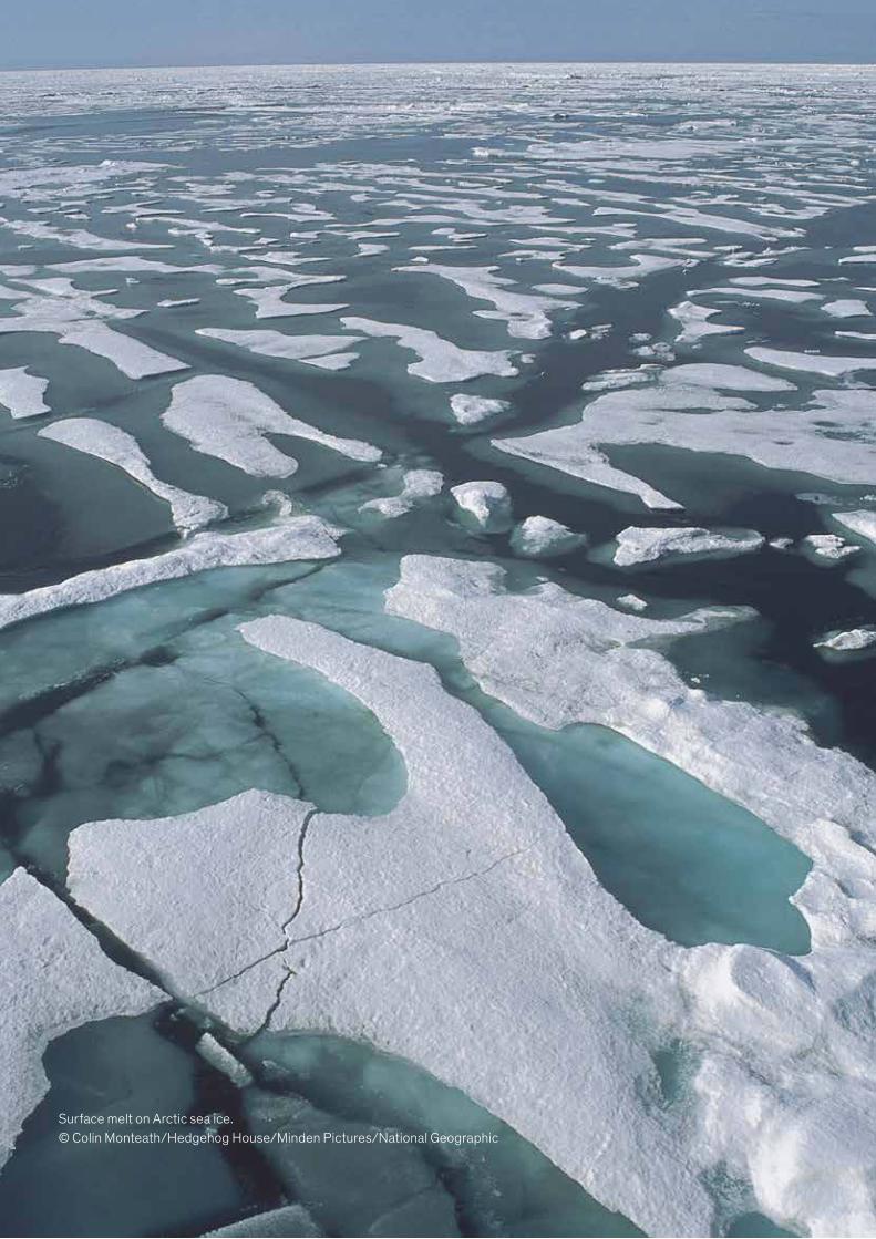
Surface melt on Arctic sea ice. © Colin Monteath/Hedgehog House/Minden Pictures/National Geographic

Contents
In brief viii
Executive summary 1
1. Understanding physical climate risk 39
2. A changing climate and resulting physical risk 49
3. Physical climate risk—a micro view 61
4. Physical climate risk—a macro view 89
5. An effective response 113
Glossary of terms 121
Technical appendix 123
Bibliography 141
viiClimate risk and response: Physical hazards and socioeconomic impacts
In brief
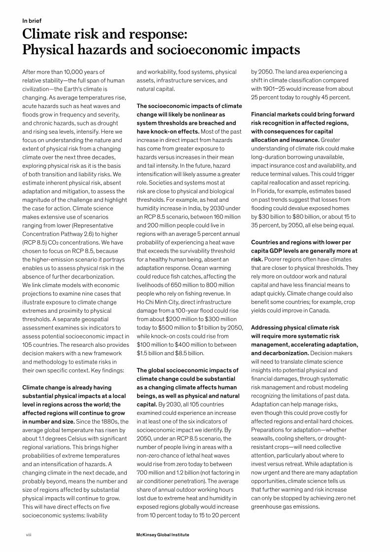
Climate risk and response: Physical hazards and socioeconomic impactsAfter more than 10,000 years of relative stability—the full span of human civilization—the Earth’s climate is changing. As average temperatures rise, acute hazards such as heat waves and floods grow in frequency and severity, and chronic hazards, such as drought and rising sea levels, intensify. Here we focus on understanding the nature and extent of physical risk from a changing climate over the next three decades, exploring physical risk as it is the basis of both transition and liability risks. We estimate inherent physical risk, absent adaptation and mitigation, to assess the magnitude of the challenge and highlight the case for action. Climate science makes extensive use of scenarios ranging from lower (Representative Concentration Pathway 2.6) to higher (RCP 8.5) CO2 concentrations. We have chosen to focus on RCP 8.5, because the higher-emission scenario it portrays enables us to assess physical risk in the absence of further decarbonization. We link climate models with economic projections to examine nine cases that illustrate exposure to climate change extremes and proximity to physical thresholds. A separate geospatial assessment examines six indicators to assess potential socioeconomic impact in 105 countries. The research also provides decision makers with a new framework and methodology to estimate risks in their own specific context. Key findings:
Climate change is already having substantial physical impacts at a local level in regions across the world; the affected regions will continue to grow in number and size. Since the 1880s, the average global temperature has risen by about 1.1 degrees Celsius with significant regional variations. This brings higher probabilities of extreme temperatures and an intensification of hazards. A changing climate in the next decade, and probably beyond, means the number and size of regions affected by substantial physical impacts will continue to grow. This will have direct effects on five socioeconomic systems: livability
and workability, food systems, physical assets, infrastructure services, and natural capital.
The socioeconomic impacts of climate change will likely be nonlinear as system thresholds are breached and have knock-on effects. Most of the past increase in direct impact from hazards has come from greater exposure to hazards versus increases in their mean and tail intensity. In the future, hazard intensification will likely assume a greater role. Societies and systems most at risk are close to physical and biological thresholds. For example, as heat and humidity increase in India, by 2030 under an RCP 8.5 scenario, between 160 million and 200 million people could live in regions with an average 5 percent annual probability of experiencing a heat wave that exceeds the survivability threshold for a healthy human being, absent an adaptation response. Ocean warming could reduce fish catches, affecting the livelihoods of 650 million to 800 million people who rely on fishing revenue. In Ho Chi Minh City, direct infrastructure damage from a 100-year flood could rise from about $200 million to $300 million today to $500 million to $1 billion by 2050, while knock-on costs could rise from $100 million to $400 million to between $1.5 billion and $8.5 billion.
The global socioeconomic impacts of climate change could be substantial as a changing climate affects human beings, as well as physical and natural capital. By 2030, all 105 countries examined could experience an increase in at least one of the six indicators of socioeconomic impact we identify. By 2050, under an RCP 8.5 scenario, the number of people living in areas with a non-zero chance of lethal heat waves would rise from zero today to between 700 million and 1.2 billion (not factoring in air conditioner penetration). The average share of annual outdoor working hours lost due to extreme heat and humidity in exposed regions globally would increase from 10 percent today to 15 to 20 percent
by 2050. The land area experiencing a shift in climate classification compared with 1901–25 would increase from about 25 percent today to roughly 45 percent.
Financial markets could bring forward risk recognition in affected regions, with consequences for capital allocation and insurance. Greater understanding of climate risk could make long-duration borrowing unavailable, impact insurance cost and availability, and reduce terminal values. This could trigger capital reallocation and asset repricing. In Florida, for example, estimates based on past trends suggest that losses from flooding could devalue exposed homes by $30 billion to $80 billion, or about 15 to 35 percent, by 2050, all else being equal.
Countries and regions with lower per capita GDP levels are generally more at risk. Poorer regions often have climates that are closer to physical thresholds. They rely more on outdoor work and natural capital and have less financial means to adapt quickly. Climate change could also benefit some countries; for example, crop yields could improve in Canada.
Addressing physical climate risk will require more systematic risk management, accelerating adaptation, and decarbonization. Decision makers will need to translate climate science insights into potential physical and financial damages, through systematic risk management and robust modeling recognizing the limitations of past data. Adaptation can help manage risks, even though this could prove costly for affected regions and entail hard choices. Preparations for adaptation—whether seawalls, cooling shelters, or drought-resistant crops—will need collective attention, particularly about where to invest versus retreat. While adaptation is now urgent and there are many adaptation opportunities, climate science tells us that further warming and risk increase can only be stopped by achieving zero net greenhouse gas emissions.
viii McKinsey Global Institute
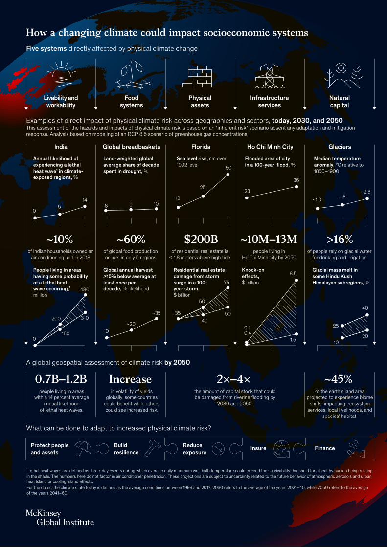
How a changing climate could impact socioeconomic systemsFive systems directly a�ected by physical climate change
Examples of direct impact of physical climate risk across geographies and sectors, today, 2030, and 2050This assessment of the hazards and impacts of physical climate risk is based on an "inherent risk" scenario absent any adaptation and mitigation response. Analysis based on modeling of an RCP 8.5 scenario of greenhouse gas concentrations.
A global geospatial assessment of climate risk by 2050
~10%
Livability andworkability
Foodsystems
Physicalassets
Infrastructureservices
Naturalcapital
India Global breadbaskets Florida Ho Chi Minh City Glaciers
Annual likelihood ofexperiencing a lethalheat wave¹ in climate-exposed regions, %
of Indian households owned anair conditioning unit in 2018
~60% of global food productionoccurs in only 5 regions
>16% of people rely on glacial water
for drinking and irrigation
$200Bof residential real estate is
< 1.8 meters above high tide
~10M–13M people living in
Ho Chi Minh city by 2050
0.7B–1.2B
Land-weighted globalaverage share of decadespent in drought, %
Sea level rise, cm over1992 level
Flooded area of city in a 100-year �ood, %
Median temperatureanomaly, °C relative to1850–1900
People living in areashaving some probabilityof a lethal heatwave occurring,¹million
Global annual harvest>15% below average atleast once perdecade, % likelihood
Residential real estatedamage from stormsurge in a 100-year storm,$ billion
Knock-one�ects,$ billion
Glacial mass melt insome Hindu KushHimalayan subregions, %
05
14
0
200
160
480
310
8 109
10~20
~35 35
50
40
75
50
0.1-0.4
8.5
1.5
25
10
40
20
1223
~1.0 ~1.5~2.3
3625
50
people living in areaswith a 14 percent average
annual likelihoodof lethal heat waves.
For the dates, the climate state today is de�ned as the average conditions between 1998 and 2017, 2030 refers to the average of the years 2021–40, while 2050 refers to the average of the years 2041–60.
¹Lethal heat waves are de�ned as three-day events during which average daily maximum wet-bulb temperature could exceed the survivability threshold for a healthy human being resting in the shade. The numbers here do not factor in air conditioner penetration. These projections are subject to uncertainty related to the future behavior of atmospheric aerosols and urban heat island or cooling island e�ects.
in volatility of yields globally, some countries
could bene�t while others could see increased risk.
2×–4×Increasethe amount of capital stock that could be damaged from riverine �ooding by
2030 and 2050.
~45%of the earth’s land area
projected to experience biome shifts, impacting ecosystem
services, local livelihoods, and species' habitat.
What can be done to adapt to increased physical climate risk?
Protect peopleand assets
Buildresilience
Reduceexposure
Insure Finance

Coping with rising temperatures in Singapore. © Getty Images
McKinsey has a long history of research on topics related to the economics of climate change. Over the past decade, we have published a variety of research including a cost curve illustrating feasible approaches to abatement and reports on understanding the economics of adaptation and identifying the potential to improve resource productivity.1 This research builds on that work and focuses on understanding the nature and implications of physical climate risk in the next three decades.
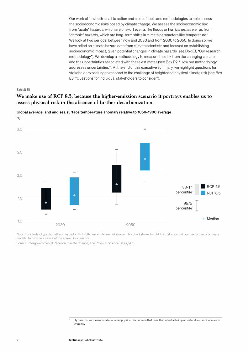
We draw on climate model forecasts to showcase how the climate has changed and could continue to change, how a changing climate creates new risks and uncertainties, and what steps can be taken to best manage them. Climate impact research makes extensive use of scenarios. Four “Representative Concentration Pathways“ (RCPs) act as standardized inputs to climate models. They outline different atmospheric greenhouse gas concentration trajectories between 2005 and 2100. During their inception, RCPs were designed to collectively sample the range of then-probable future emission pathways, ranging from lower (RCP2.6) to higher (RCP 8.5) CO2 concentrations. Each RCP was created by an independent modeling team and there is no consistent design of the socio-economic parameter assumptions used in the derivation of the RCPs. By 2100, the four RCPs lead to very different levels of warming, but the divergence is moderate out to 2050 and small to 2030. Since the research in this report is most concerned with understanding inherent physical risks, we have chosen to focus on the higher-emission scenario, i.e. RCP 8.5, because of the higher-emissions, lower-mitigation scenario it portrays, in order to assess physical risk in absence of further decarbonization (Exhibit E1).
We focus on physical risk—that is, the risks arising from the physical effects of climate change, including the potential effects on people, communities, natural and physical capital, and economic activity, and the implications for companies, governments, financial institutions, and individuals. Physical risk is the fundamental driver of other climate risk types—transition risk and liability risk.2 We do not focus on transition risks, that is, impacts from decarbonization, or liability risks associated with climate change. While an understanding of decarbonization and the risk and opportunities it creates is a critical topic, this report contributes by exploring the nature and costs of ongoing climate change in the next one to three decades in the absence of decarbonization.
1 See, for example, Shaping climate-resilient development: A framework for decision-making, Economics of Climate Adaptation, 2009; “Mapping the benefits of the circular economy,” McKinsey Quarterly, June 2017; Resource revolution: Meeting the world’s energy, materials, food, and water needs, McKinsey Global Institute, November 2011; and Beyond the supercycle: How technology is reshaping resources, McKinsey Global Institute, February 2017. For details of the abatement cost curves, see Greenhouse gas abatement cost curves, McKinsey.com.
2 Transition risk can be defined as risks arising from transition to a low-carbon economy; liability risk as risks arising from those affected by climate change seeking compensation for losses. See Climate change: What are the risks to financial stability? Bank of England, KnowledgeBank.
Executive summary
1Climate risk and response: Physical hazards and socioeconomic impacts
Our work offers both a call to action and a set of tools and methodologies to help assess the socioeconomic risks posed by climate change. We assess the socioeconomic risk from “acute” hazards, which are one-off events like floods or hurricanes, as well as from “chronic” hazards, which are long-term shifts in climate parameters like temperature.3 We look at two periods: between now and 2030 and from 2030 to 2050. In doing so, we have relied on climate hazard data from climate scientists and focused on establishing socioeconomic impact, given potential changes in climate hazards (see Box E1, “Our research methodology”). We develop a methodology to measure the risk from the changing climate and the uncertainties associated with these estimates (see Box E2, “How our methodology addresses uncertainties”). At the end of this executive summary, we highlight questions for stakeholders seeking to respond to the challenge of heightened physical climate risk (see Box E3, “Questions for individual stakeholders to consider”).
3 By hazards, we mean climate-induced physical phenomena that have the potential to impact natural and socioeconomic systems.
Exhibit E1
We make use of RCP 8.5, because the higher-emission scenario it portrays enables us to assess physical risk in the absence of further decarbonization.
Source: Intergovernmental Panel on Climate Change, The Physical Science Basis, 2013
Global average land and sea surface temperature anomaly relative to 1850–1900 average°C
1.0
1.5
2.0
2.5
3.0
2030 2050
RCP 4.5RCP 8.5
83/17 percentile
95/5 percentile
Median
NOTE!
All exh that repeat from case studies, use case exh as definitive.
All exh that repeat in ES, use report as
definitive.
Note: For clarity of graph, outliers beyond 95th to 5th percentile are not shown. This chart shows two RCPs that are most commonly used in climate models, to provide a sense of the spread in scenarios.
2 McKinsey Global Institute

Box E1 Our research methodology
In this report, we measure the impact of climate change by the extent to which it could affect human beings, human-made physical assets, and the natural world. While many scientists, including climate scientists, are employed at McKinsey & Company, we are not a climate modeling institution. Our focus in this report has been on translating the climate science data into an assessment of physical risk and its implications for stakeholders. Most of the climatological analysis performed for this report was done by Woods Hole Research Center (WHRC), and in other instances, we relied on publicly available climate science data, for example from institutions like the World Resources Institute. WHRC’s work draws on the most widely used and thoroughly peer-reviewed ensemble of climate models to estimate the probabilities of relevant climate events occurring. Here, we highlight key methodological choices:
Case studiesIn order to link physical climate risk to socioeconomic impact, we investigate nine specific cases that illustrate exposure to climate change extremes and proximity to physical thresholds. These cover a range of sectors and geographies and provide the basis of a “micro-to-macro” approach that is a characteristic of MGI research. To inform our selection of cases, we considered over 30 potential combinations of climate hazards, sectors, and geographies based on a review of the literature and expert interviews on the potential direct impacts of physical climate hazards. We find these hazards affect five different key socioeconomic systems: livability and workability, food systems, physical assets, infrastructure services, and natural capital.
We ultimately chose nine cases to reflect these systems and based on their exposure to the extremes of climate change and their proximity today to key physiological, human-made, and ecological thresholds. As such, these cases represent leading-edge examples of climate change risk. They show that the direct risk from climate hazards is determined by the severity of the hazard and its likelihood, the exposure of various “stocks” of capital (people, physical capital, and natural capital) to these hazards, and the resilience of these stocks to the hazards (for example, the ability of physical assets to withstand flooding). Through our case studies, we also assess the knock-on effects that could occur, for example to downstream sectors or consumers. We primarily rely on past examples and empirical estimates for this assessment of knock-on effects, which is likely not exhaustive given the complexities associated with socioeconomic systems. Through this “micro” approach, we offer decision makers a methodology by which to assess direct physical climate risk, its characteristics, and its potential knock-on impacts.
Global geospatial analysisIn a separate analysis, we use geospatial data to provide a perspective on climate change across 105 countries over the next 30 years. This geospatial analysis relies on the same five-systems framework of direct impacts that we used for the case studies. For each of these systems, we identify a measure, or measures, of the impact of climate change, using indicators where possible as identified in our cases.
Similar to the approach discussed above for our cases, our analyses are conducted at a grid-cell level, overlaying data on a hazard (for example, floods of different depths, with their associated likelihoods), with exposure to that hazard (for example, capital stock exposed to flooding), and a damage function that assesses resilience (for example, what share of capital stock is damaged when exposed to floods of different depth). We then combine these grid-cell values to country and global numbers. While the goal of this analysis is to measure direct impact, due to data availability issues, we have used five measures of socioeconomic impact and one measure of climate hazards themselves—drought. Our set of 105 countries represents 90 percent of the world’s population and 90 percent of global GDP. While we seek
3Climate risk and response: Physical hazards and socioeconomic impacts

to include a wide range of risks and as many countries as possible, there are some we could not cover due to data limitations (for example, the impact of forest fires and storm surges).
What this report does not doSince the purpose of this report is to understand the physical risks and disruptive impacts of climate change, there are many areas which we do not address.
— We do not assess the efficacy of climate models but instead draw on best practice approaches from climate science literature and highlight key uncertainties.
— We do not examine in detail areas and sectors that are likely to benefit from climate change such as the potential for improved agricultural yields in parts of Canada, although we quantify some of these benefits through our geospatial analysis.
— As the consequences of physical risk are realized, there will likely be acts of adaptation, with a feedback effect on the physical risk. For each of our cases, we identify adaptation responses. We have not conducted a detailed bottom-up cost-benefit analysis of adaptation but have built on existing literature and expert interviews to understand the most important measures and their indicative cost, effectiveness, and implementation challenges, and to estimate the expected global adaptation spending required.
— We note the critical importance of decarbonization in a climate risk management approach but a detailed discussion of decarbonization is beyond the scope of this report.
— While we attempt to draw out qualitatively (and, to the extent possible, quantitatively) the knock-on effects from direct physical impacts of climate change, we recognize the limitations of this exercise given the complexity of socioeconomic systems. There are likely knock-on effects that could occur which our analysis has not taken into account. For this reason, we do not attempt to size the global GDP at risk from climate change (see Box 4 in Chapter 4 for a detailed discussion).
— We do not provide projections or deterministic forecasts, but rather assess risk. The climate is the statistical summary of weather patterns over time and is therefore probabilistic in nature. Following standard practice, our findings are therefore framed as “statistically expected values”—the statistically expected average impact across a range of probabilities of higher or lower climate outcomes.1
1 We also report the value of “tail risks”—that is, low-probability, high-impact events like a 1-in-100-year storm—on both an annual and cumulative basis. Consider, for example, a flooding event that has a 1 percent annual likelihood of occurrence every year (often described as a “100-year flood”). In the course of the lifetime of home ownership—for example, over a 30-year period—the cumulative likelihood that the home will experience at least one 100-year flood is 26 percent.
4 McKinsey Global Institute
Box E2How our methodology addresses uncertainties
1 See Naomi Oreskes and Nicholas Stern, “Climate change will cost us even more than we think,” New York Times, October 23, 2019.
One of the main challenges in understanding the physical risk arising from climate change is the range of uncertainties involved. Risks arise as a result of an involved causal chain. Emissions influence both global climate and regional climate variations, which in turn influence the risk of specific climate hazards (such as droughts and sea-level rise), which then influence the risk of physical damage (such as crop shortages and infrastructure damages), which finally influence the risk of financial harm. Our analysis, like any such effort, relies on assumptions made along the causal chain: about emission paths and adaptation schemes; global and regional climate models; physical damage functions; and knock-on effects. The further one goes along the chain, the greater the intrinsic model uncertainty.
Taking a risk-management lens, we have developed a methodology to provide decision makers with an outlook over the next three decades on the inherent risk of climate change—that is, risk absent any adaptation and mitigation response. Separately, we outline how this risk could be reduced via an adaptation response in our case studies. Where feasible, we have attempted to size the costs of the potential adaptation responses. We
believe this approach is appropriate to help stakeholders understand the potential magnitude of the impacts from climate change and the commensurate response required.
The key uncertainties include the emissions pathway and pace of warming, climate model accuracy and natural variability, the magnitude of direct and indirect socioeconomic impacts, and the socioeconomic response. Assessing these uncertainties, we find that our approach likely results in conservative estimates of inherent risk because of the skew in uncertainties of many hazard projections toward “worse” outcomes as well as challenges with modeling the many potential knock-on effects associated with direct physical risk.1
Emissions pathway and pace of warmingAs noted above, we have chosen to focus on the RCP 8.5 scenario because the higher-emission scenario it portrays enables us to assess physical risk in the absence of further decarbonization. Under this scenario, science tells us that global average temperatures will reach just over 2 degrees Celsius above preindustrial levels by 2050. However, action to reduce emissions could mean that the projected outcomes—both
hazards and impacts—based on this trajectory are delayed post 2050. For example, RCP 8.5 predicts global average warming of 2.3 degrees Celsius by 2050, compared with 1.8 degrees Celsius for RCP 4.5. Under RCP 4.5, 2.3 degrees Celsius warming would be reached in the year 2080.
Climate model accuracy and natural variabilityWe have drawn on climate science that provides sufficiently robust results, especially over a 30-year period. To minimize the uncertainty associated with any particular climate model, the mean or median projection (depending on the specific variable being modeled) from an ensemble of climate models has been used, as is standard practice in the climate literature. We also note that climate model uncertainty on global temperature increases tends to skew toward worse outcomes; that is, differences across climate models tend to predict outcomes that are skewed toward warmer rather than cooler global temperatures. In addition, the climate models used here omit potentially important biotic feedbacks including greenhouse gas emissions from thawing permafrost, which will tend to increase warming.
5Climate risk and response: Physical hazards and socioeconomic impacts

To apply global climate models to regional analysis, we used techniques established in climate literature.2 The remaining uncertainty related to physical change is variability resulting from mechanisms of natural rather than human origin. This natural climate variability, which arises primarily from multiyear patterns in ocean and/or atmosphere circulation (for example, the El Niño/La Niña oscillation), can temporarily affect global or regional temperature, precipitation, and other climatic variables. Natural variability introduces uncertainty surrounding how hazards could evolve because it can temporarily accelerate or delay the manifestation of statistical climate shifts.3 This uncertainty will be particularly important over the next decade, during which overall climatic shifts relative to today may be smaller in magnitude than an acceleration or delay in warming due to natural variability.
Direct and indirect socioeconomic impactsOur findings related to socioeconomic impact of a given physical climate effect involve uncertainty, and we have provided conservative estimates. For direct impacts, we have relied on publicly available vulnerability assessments, but they may not accurately represent the vulnerability of a specific asset or location. For indirect impacts, given the complexity
2 See technical appendix for details.3 Kyle L. Swanson, George Sugihara, and Anastasios A. Tsonis, “Long-term natural variability and 20th century climate change,” Proceedings of the National
Academy of Sciences, September 2009, Volume 106, Number 38.
of socioeconomic systems, we know that our results do not capture the full impact of climate change knock-on effects. In many cases, we have either discussed knock-on effects in a qualitative manner alone or relied on empirical estimations. This may underestimate the direct impacts of climate change’s inherent risk in our cases, for example the knock-on effects of flooding in Ho Chi Minh City or the potential for financial devaluation in Florida real estate. This is not an issue in our 105-country geospatial analysis, as the impacts we are looking at there are direct and as such we have relied on publicly available vulnerability assessments as available at a regional or country level.
Socioeconomic responseThe amount of risk that manifests also depends on the response to the risk. Adaptation measures such as hardening physical infrastructure, relocating people and assets, and ensuring backup capacity, among others, can help manage the impact of climate hazards and reduce risk. We follow an approach that first assesses the inherent risk and then considers a potential adaptation response. The inherent or ex ante level of risk is the risk without taking any steps to reduce its likelihood or severity. We have not conducted a detailed bottom-up cost-benefit analysis of adaptation measures
but have built on existing literature and expert interviews to understand the most important measures and their indicative cost, effectiveness, and implementation challenges in each of our cases, and to estimate the expected global adaptation spending required. While we note the critical importance of decarbonization in an appropriate climate risk management approach, a detailed discussion of decarbonization is beyond the scope of this report.
How decision makers incorporate these uncertainties into their management choices will depend on their risk appetite and overall risk-management approach. Some may want to work with the outcome considered most likely (which is what we generally considered), while others may want to consider a worse- or even worst-case scenario. Given the complexities we have outlined above, we recognize that more research is needed in this critical field. However, we believe that despite the many uncertainties associated with estimates of impact from a changing climate, it is possible for the science and socioeconomic analysis to provide actionable insights for decision makers. For an in-depth discussion of the main uncertainties and how we have sought to resolve them, see Chapter 1.
6 McKinsey Global Institute
We find that risk from climate change is already present and growing. The insights from our cases help highlight the nature of this risk, and therefore how stakeholders should think about assessing and managing it. Seven characteristics stand out. Physical climate risk is:
— Increasing. In each of our nine cases, the level of physical climate risk increases by 2030 and further by 2050. Across our cases, we find increases in socioeconomic impact of between roughly two and 20 times by 2050 versus today’s levels. We also find physical climate risks are generally increasing across our global country analysis even as some countries find some benefits (such as increased agricultural yields in Canada, Russia, and parts of northern Europe).
— Spatial. Climate hazards manifest locally. The direct impacts of physical climate risk thus need to be understood in the context of a geographically defined area. There are variations between countries and also within countries.
— Non-stationary. As the Earth continues to warm, physical climate risk is ever-changing or non-stationary. Climate models and basic physics predict that further warming is “locked in” over the next decade due to inertia in the geophysical system, and that the temperature will likely continue to increase for decades to come due to socio-technological inertia in reducing emissions.4 Climate science tells us that further warming and risk increase can only be stopped by achieving zero net greenhouse gas emissions. Furthermore, given the thermal inertia of the earth system, some amount of warming will also likely occur after net-zero emissions are reached.5 Managing that risk will thus require not moving to a “new normal” but preparing for a world of constant change. Financial markets, companies, governments, or individuals have mostly not had to address being in an environment of constant change before, and decision making based on experience may no longer be reliable. For example, engineering parameters for infrastructure design in certain locations will need to be re-thought, and home owners may need to adjust assumptions about taking on long-term mortgages in certain geographies.
— Nonlinear. Socioeconomic impacts are likely to propagate in a nonlinear way as hazards reach thresholds beyond which the affected physiological, human-made, or ecological systems work less well or break down and stop working altogether. This is because such systems have evolved or been optimized over time for historical climates. Consider, for example, buildings designed to withstand floods of a certain depth, or crops grown in regions with a specific climate. While adaptation in theory can be carried out at a fairly rapid rate for some systems (for example, improving the floodproofing of a factory), the current rate of warming—which is at least an order of magnitude faster than any found in the past 65 million years of paleoclimate records—means that natural systems such as crops are unable to evolve fast enough to keep pace.6 Impacts could be significant if system thresholds are breached even by small amounts. The occurrence of multiple risk factors (for example, exposure to multiple hazards, other vulnerabilities like the ability to finance adaptation investments, or high reliance on a sector that is exposed to climate hazard) in a single geography, something we see in several of our cases, is a further source of potential nonlinearity.
— Systemic. While the direct impact from climate change is local, it can have knock-on effects across regions and sectors, through interconnected socioeconomic and financial systems. For example, flooding in Florida could not only damage housing but also raise insurance costs, affect property values of exposed homes, and in turn reduce property tax revenues
4 H. Damon Matthews et al., “Focus on cumulative emissions, global carbon budgets, and the implications for climate mitigation targets,” Environmental Research Letters, January 2018, Volume 13, Number 1.
5 H. Damon Matthews et al., “Focus on cumulative emissions, global carbon budgets, and the implications for climate mitigation targets,” Environmental Research Letters, January 2018, Volume 13, Number 1; H. Damon Matthews & Ken Caldeira, “Stabilizing climate requires near zero emissions”. Geophysical Research Letters February 2008, Volume 35; Myles Allen et al, “Warming caused by cumulative carbon emissions towards the trillionth ton.” Nature, April 2009, Volume 485.
6 Noah S. Diffenbaugh and Christopher B. Field, “Changes in ecologically critical terrestrial climate conditions,” Science, August 2013, Volume 341, Number 6145; Seth D. Burgess, Samuel Bowring, and Shu-zhong Shen, “High-precision timeline for Earth’s most severe extinction,” Proceedings of the National Academy of Sciences, March 2014, Volume 111, Number 9.
7Climate risk and response: Physical hazards and socioeconomic impacts
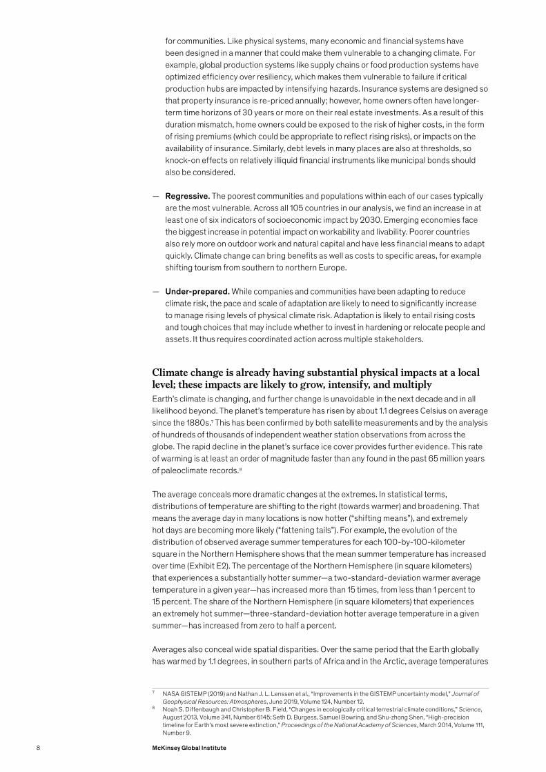
for communities. Like physical systems, many economic and financial systems have been designed in a manner that could make them vulnerable to a changing climate. For example, global production systems like supply chains or food production systems have optimized efficiency over resiliency, which makes them vulnerable to failure if critical production hubs are impacted by intensifying hazards. Insurance systems are designed so that property insurance is re-priced annually; however, home owners often have longer-term time horizons of 30 years or more on their real estate investments. As a result of this duration mismatch, home owners could be exposed to the risk of higher costs, in the form of rising premiums (which could be appropriate to reflect rising risks), or impacts on the availability of insurance. Similarly, debt levels in many places are also at thresholds, so knock-on effects on relatively illiquid financial instruments like municipal bonds should also be considered.
— Regressive. The poorest communities and populations within each of our cases typically are the most vulnerable. Across all 105 countries in our analysis, we find an increase in at least one of six indicators of socioeconomic impact by 2030. Emerging economies face the biggest increase in potential impact on workability and livability. Poorer countries also rely more on outdoor work and natural capital and have less financial means to adapt quickly. Climate change can bring benefits as well as costs to specific areas, for example shifting tourism from southern to northern Europe.
— Under-prepared. While companies and communities have been adapting to reduce climate risk, the pace and scale of adaptation are likely to need to significantly increase to manage rising levels of physical climate risk. Adaptation is likely to entail rising costs and tough choices that may include whether to invest in hardening or relocate people and assets. It thus requires coordinated action across multiple stakeholders.
Climate change is already having substantial physical impacts at a local level; these impacts are likely to grow, intensify, and multiply Earth’s climate is changing, and further change is unavoidable in the next decade and in all likelihood beyond. The planet’s temperature has risen by about 1.1 degrees Celsius on average since the 1880s.7 This has been confirmed by both satellite measurements and by the analysis of hundreds of thousands of independent weather station observations from across the globe. The rapid decline in the planet’s surface ice cover provides further evidence. This rate of warming is at least an order of magnitude faster than any found in the past 65 million years of paleoclimate records.8
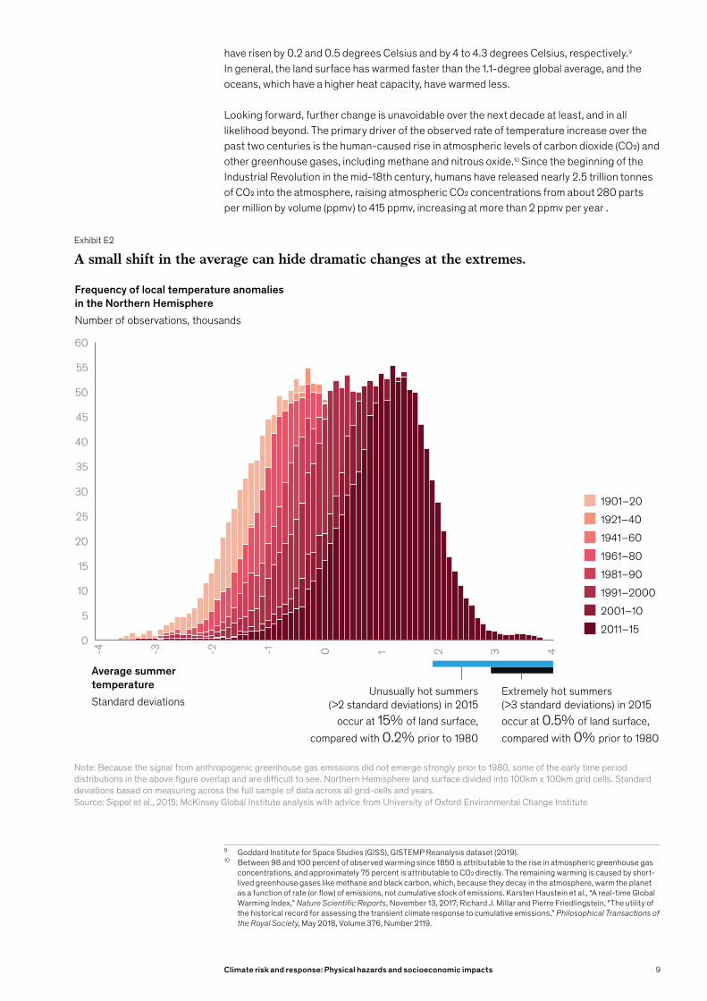
The average conceals more dramatic changes at the extremes. In statistical terms, distributions of temperature are shifting to the right (towards warmer) and broadening. That means the average day in many locations is now hotter (“shifting means”), and extremely hot days are becoming more likely (“fattening tails”). For example, the evolution of the distribution of observed average summer temperatures for each 100-by-100-kilometer square in the Northern Hemisphere shows that the mean summer temperature has increased over time (Exhibit E2). The percentage of the Northern Hemisphere (in square kilometers) that experiences a substantially hotter summer—a two-standard-deviation warmer average temperature in a given year—has increased more than 15 times, from less than 1 percent to 15 percent. The share of the Northern Hemisphere (in square kilometers) that experiences an extremely hot summer—three-standard-deviation hotter average temperature in a given summer—has increased from zero to half a percent.
Averages also conceal wide spatial disparities. Over the same period that the Earth globally has warmed by 1.1 degrees, in southern parts of Africa and in the Arctic, average temperatures
7 NASA GISTEMP (2019) and Nathan J. L. Lenssen et al., “Improvements in the GISTEMP uncertainty model,” Journal of Geophysical Resources: Atmospheres, June 2019, Volume 124, Number 12.
8 Noah S. Diffenbaugh and Christopher B. Field, “Changes in ecologically critical terrestrial climate conditions,” Science, August 2013, Volume 341, Number 6145; Seth D. Burgess, Samuel Bowring, and Shu-zhong Shen, “High-precision timeline for Earth’s most severe extinction,” Proceedings of the National Academy of Sciences, March 2014, Volume 111, Number 9.
8 McKinsey Global Institute
have risen by 0.2 and 0.5 degrees Celsius and by 4 to 4.3 degrees Celsius, respectively.9 In general, the land surface has warmed faster than the 1.1-degree global average, and the oceans, which have a higher heat capacity, have warmed less.
Looking forward, further change is unavoidable over the next decade at least, and in all likelihood beyond. The primary driver of the observed rate of temperature increase over the past two centuries is the human-caused rise in atmospheric levels of carbon dioxide (CO2) and other greenhouse gases, including methane and nitrous oxide.10 Since the beginning of the Industrial Revolution in the mid-18th century, humans have released nearly 2.5 trillion tonnes of CO2 into the atmosphere, raising atmospheric CO2 concentrations from about 280 parts per million by volume (ppmv) to 415 ppmv, increasing at more than 2 ppmv per year .
9 Goddard Institute for Space Studies (GISS), GISTEMP Reanalysis dataset (2019).10 Between 98 and 100 percent of observed warming since 1850 is attributable to the rise in atmospheric greenhouse gas
concentrations, and approximately 75 percent is attributable to CO2 directly. The remaining warming is caused by short-lived greenhouse gases like methane and black carbon, which, because they decay in the atmosphere, warm the planet as a function of rate (or flow) of emissions, not cumulative stock of emissions. Karsten Haustein et al., “A real-time Global Warming Index,” Nature Scientific Reports, November 13, 2017; Richard J. Millar and Pierre Friedlingstein, “The utility of the historical record for assessing the transient climate response to cumulative emissions,” Philosophical Transactions of the Royal Society, May 2018, Volume 376, Number 2119.
Exhibit E2
A small shift in the average can hide dramatic changes at the extremes.
20
0
5
10
35
15
25
30
40
50
45
55
60
-3
Average summer temperatureStandard deviations
Frequency of local temperature anomalies in the Northern HemisphereNumber of observations, thousands
-4 -2 -1 0 41 2 3
Source: Sippel et al., 2015; McKinsey Global Institute analysis with advice from University of Oxford Environmental Change Institute
Note: Because the signal from anthropogenic greenhouse gas emissions did not emerge strongly prior to 1980, some of the early time period distributions in the above figure overlap and are difficult to see. Northern Hemisphere land surface divided into 100km x 100km grid cells. Standard deviations based on measuring across the full sample of data across all grid-cells and years.
1901–201921–40
1961–801941–60
2011–15
1981–901991–20002001–10
Unusually hot summers (>2 standard deviations) in 2015
occur at 15% of land surface, compared with 0.2% prior to 1980
Extremely hot summers (>3 standard deviations) in 2015 occur at 0.5% of land surface, compared with 0% prior to 1980
9Climate risk and response: Physical hazards and socioeconomic impacts

Carbon dioxide persists in the atmosphere for hundreds of years.11 As a result, in the absence of large-scale human action to remove CO2 from the atmosphere, nearly all of the warming that occurs will be permanent on societally relevant timescales.12 Additionally, because of the strong thermal inertia of the ocean, more warming is likely already locked in over the next decade, regardless of emissions pathway. Beyond 2030, climate science tells us that further warming and risk increase can only be stopped by achieving zero net greenhouse gas emissions.13
With increases in global average temperatures, climate models indicate a rise in climate hazards globally. According to climate science, further warming will continue to increase the frequency and/or severity of acute climate hazards across the world, such as lethal heat waves, extreme precipitation, and hurricanes, and will further intensify chronic hazards such as drought, heat stress, and rising sea levels.14 Here, we describe the prediction of climate models analyzed by WHRC, and also publicly available data for a selection of hazards for an RCP 8.5 scenario (Exhibits E3 and E4):
— Increase in average temperatures.15 Global average temperatures are expected to increase over the next three decades, resulting in a 2.3-degree Celsius (+0.5/-0.3) average increase relative to the preindustrial period by 2050, under an RCP 8.5 scenario. Depending on the exact location, this can translate to an average local temperature increase of between 1.5 and 5.0 degrees Celsius relative to today. The Arctic in particular is expected to warm more rapidly than elsewhere.
— Extreme precipitation.16 In parts of the world, extreme precipitation events, defined here as one that was a once in a 50-year event (that is, with a 2 percent annual likelihood) in the 1950–81 period, are expected to become more common. The likelihood of extreme precipitation events is expected to grow more than fourfold in some regions, including parts of China, Central Africa, and the east coast of North America compared with the period 1950–81.
— Hurricanes.17 While climate change is seen as unlikely to alter the frequency of tropical hurricanes, climate models and basic physical theory predict an increase in the average severity of those storms (and thus an increase in the frequency of severe hurricanes). The likelihood of severe hurricane precipitation—that is, an event with a 1 percent likelihood annually in the 1981–2000 period—is expected to double in some parts of the southeastern United States and triple in some parts of Southeast Asia by 2040. Both are densely populated areas with large and globally connected economic activity.
— Drought.18 As the Earth warms, the spatial extent and share of time spent in drought is projected to increase. The share of a decade spent in drought conditions is projected to be up to 80 percent in some parts of the world by 2050, notably in parts of the Mediterranean, southern Africa, and Central and South America.
11 David Archer. “Fate of Fossil Fuel CO2 in geological time.” Journal of Geophysical Research, March 2005, Volume 110.12 H. Damon Matthews et al., “Focus on cumulative emissions, global carbon budgets, and the implications for climate
mitigation targets,” Environmental Research Letters, January 2018, Volume 13, Number 1. David Archer. “Fate of Fossil Fuel CO2 in geological time.” Journal of Geophysical Research, March 2005, Volume 110; H. Damon Matthews & Susan Solomon. “Irreversible does not mean unavoidable.” Science. April 2013, Volume 340, Issue 6131.
13 H. Damon Matthews et al., “Focus on cumulative emissions, global carbon budgets, and the implications for climate mitigation targets,” Environmental Research Letters, January 2018, Volume 13, Number 1; H. Damon Matthews & Ken Caldeira, “Stabilizing climate requires near zero emissions”. Geophysical Research Letters February 2008, Volume 35; Myles Allen et al, “Warming caused by cumulative carbon emissions towards the trillionth ton.” Nature, April 2009, Volume 485.
14 This list of climate hazards is a subset, and the full list can be found in the full report. The list is illustrative rather than exhaustive. Due to data and modeling constraints, we did not include the following hazards: increased frequency and severity of forest fires, increased biological and ecological impacts from pests and diseases, increased severity of hurricane wind speed and storm surge, and more frequent and severe coastal flooding due to sea-level rise.
15 Taken from KNMI Climate Explorer (2019), using the mean of the full CMIP5 ensemble of models. 16 Modeled by WHRC using the median projection from 20 CMIP5 Global Climate Models (GCMs). To accurately estimate
the probability of extreme precipitation events, a process known as statistical bootstrapping was used. Because these projections are not estimating absolute values, but rather changes over time, bias correction was not used.
17 Modeled by WHRC using the Coupled Hurricane Intensity Prediction System (CHIPS) model from Kerry Emanuel, MIT, 2019. Time periods available for the hurricane modeling were 1981–2000 baseline, and 2031–50 future period. These are the results for two main hurricane regions of the world; other including the Indian sub-continent were not modeled.
18 Modeled by WHRC using the median projection of 20 CMIP5 GCMs, using the self-correcting Palmer Drought Severity Index (PDSI). Projections were corrected to account for increasing atmospheric CO2 concentrations.
10 McKinsey Global Institute
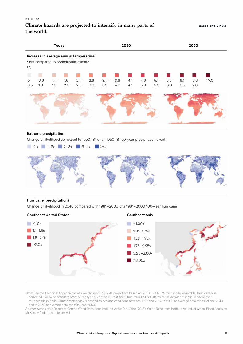
Exhibit E3
Today 2030 2050
Increase in average annual temperatureShift compared to preindustrial climate°C
Extreme precipitationChange of likelihood compared to 1950–81 of an 1950–81 50-year precipitation event
Hurricane (precipitation)Change of likelihood in 2040 compared with 1981–2000 of a 1981–2000 100-year hurricane
Climate hazards are projected to intensify in many parts of the world.
Note: See the Technical Appendix for why we chose RCP 8.5. All projections based on RCP 8.5, CMIP 5 multi model ensemble. Heat data bias corrected. Following standard practice, we typically define current and future (2030, 2050) states as the average climatic behavior over multidecade periods. Climate state today is defined as average conditions between 1998 and 2017, in 2030 as average between 2021 and 2040, and in 2050 as average between 2041 and 2060.
Source: Woods Hole Research Center; World Resources Institute Water Risk Atlas (2018); World Resources Institute Aqueduct Global Flood Analyzer; McKinsey Global Institute analysis
≤1x 1–2x 2–3x 3–4x >4x
≤1.0x
1.1–1.5x
1.6–2.0x
>2.0x
Southeast United States Southeast Asia
≤1.00x
1.01–1.25x
1.26–1.75x
1.76–2.25x
2.26–3.00x
>3.00x
Based on RCP 8.5
0–0.5
0.6–1.0
1.1–1.5
1.6–2.0
2.1–2.5
2.6–3.0
3.1–3.5
3.6–4.0
4.1–4.5
4.6–5.0
5.1–5.5
5.6–6.0
6.1–6.5
6.6–7.0
>7.0
11Climate risk and response: Physical hazards and socioeconomic impacts

Exhibit E4
Today 2030 2050
Drought frequency1
% of decade in drought
Lethal heat wave probability2
% p.a.
Water supplyChange in surface water compared with 2018 (%)Boundaries on the map represent water basins
Climate hazards are projected to intensify in many parts of the world (continued).
1. Measured using a three-month rolling average. Drought is defined as a rolling three month period with Average Palmer Drought Severity Index (PDSI) <-2. PDSI is a temperature and precipitation-based drought index calculated based on deviation from historical mean. Values generally range from +4 (extremely wet) to -4 (extremely dry).
2. A lethal heat wave is defined as a three-day period with maximum daily wet-bulb temperatures exceeding 34°C wet-bulb, where wet-bulb temperature is defined as the lowest temperature to which a parcel of air can be cooled by evaporation at constant pressure. This threshold was chosen because the commonly defined heat threshold for human survivability is 35°C wet-bulb, and large cities with significant urban heat island effects could push 34°C wet-bulb heat waves over the 35°C threshold. Under these conditions, a healthy, well-hydrated human being resting in the shade would see core body temperatures rise to lethal levels after roughly 4–5 hours of exposure. These projections are subject to uncertainty related to the future behavior of atmospheric aerosols and urban heat island or cooling island effects.
Note: See the Technical Appendix for why we chose RCP 8.5. All projections based on RCP 8.5, CMIP 5 multi model ensemble. Heat data bias corrected. Following standard practice, we typically define current and future (2030, 2050) states as the average climatic behavior over multidecade periods. Climate state today is defined as average conditions between 1998 and 2017, in 2030 as average between 2021 and 2040, and in 2050 as average between 2041 and 2060.
≤2 3–5 6–10 11–15 16–30 31–45 46–60 >60
>70% decrease
41–70% decrease
20–40% decrease
Nearnormal
20–40% increase
41–70% increase
>70% increase
Source: Woods Hole Research Center; World Resources Institute Water Risk Atlas (2018); World Resources Institute Aqueduct Global Flood Analyzer; McKinsey Global Institute analysis
Based on RCP 8.5
0 1–10 11–20 21–40 41–60 61–80 >80
12 McKinsey Global Institute

— Lethal heat waves.19 Lethal heat waves are defined as three-day events during which average daily maximum wet-bulb temperature could exceed the survivability threshold for a healthy human being resting in the shade.20 Under an RCP 8.5 scenario, urban areas in parts of India and Pakistan could be the first places in the world to experience heat waves that exceed the survivability threshold for a healthy human being, with small regions projected to experience a more than 60 percent annual chance of such a heat wave by 2050.
— Water supply.21 As rainfall patterns, evaporation, snowmelt timing, and other factors change, renewable freshwater supply will be affected. Some parts of the world like South Africa and Australia are expected to see a decrease in water supply, while other areas, including Ethiopia and parts of South America, are projected to experience an increase. Certain regions, for example, parts of the Mediterranean region and parts of the United States and Mexico, are projected to see a decrease in mean annual surface water supply of more than 70 percent by 2050. Such a large decline in water supply could cause or exacerbate chronic water stress and increase competition for resources across sectors.
The socioeconomic impacts of climate change will likely be nonlinear as system thresholds are breached and have knock-on effectsClimate change affects human life as well as the factors of production on which our economic activity is based and, by extension, the preservation and growth of wealth. We measure the impact of climate change by the extent to which it could disrupt or destroy stocks of capital—human, physical, and natural—and the resultant socioeconomic impact of that disruption or destruction. The effect on economic activity as measured by GDP is a consequence of the direct impacts on these stocks of capital.
Climate change is already having a measurable socioeconomic impact. Across the world, we find examples of these impacts and their linkage to climate change. We group these impacts in a five-systems framework (Exhibit E5). As noted in Box E1, this impact framework is our best effort to capture the range of socioeconomic impacts from physical climate hazards.
19 Modeled by WHRC using the mean projection of daily maximum surface temperature and daily mean relative humidity taken from 20 CMIP5 GCMs. Models were independently bias corrected using the ERA-Interim dataset.
20 We define a lethal heat wave as a three-day period with maximum daily wet-bulb temperatures exceeding 34 degrees Celsius wet-bulb, where wet-bulb temperature is defined as the lowest temperature to which a parcel of air can be cooled by evaporation at constant pressure. This threshold was chosen because the commonly defined heat threshold for human survivability is 35 degrees Celsius wet-bulb, and large cities with significant urban heat island effects could push 34C wet-bulb heat waves over the 35C threshold. At this temperature, a healthy human being, resting in the shade, can survive outdoors for four to five hours. These projections are subject to uncertainty related to the future behavior of atmospheric aerosols and urban heat island or cooling island effects. If a non-zero probability of lethal heat waves in certain regions occurred in the models for today, this was set to zero to account for the poor representation of the high levels of observed atmospheric aerosols in those regions in the CMIP5 models. High levels of atmospheric aerosols provide a cooling effect that masks the risk. See the India case and our technical appendix for more details. Analysis based on an RCP 8.5 scenario.
21 Taken from the World Resources Institute Water Risk Atlas (2018), which relies on 6 underlying CMIP5 models. Time periods of this raw dataset are the 20-year periods centered on 2020, 2030, and 2040. The 1998–2017 and 2041–60 data were linearly extrapolated from the 60-year trend provided in the base dataset.
13Climate risk and response: Physical hazards and socioeconomic impacts

Exhibit E5
Socioeconomic impact of climate change is already manifesting and affects all geographies.
Source: R. Garcia-Herrera et al., 2010; K. Zander et al., 2015; Yin Sun et al., 2019; Parkinson, Claire L. et al., 2013; Kirchmeier-Young, Megan C. et al., 2017; Philip, Sjoukje et al., 2018; Funk, Chris et al., 2019; ametsoc.net; Bellprat et al., 2015; cbc.ca; coast.noaa.gov; dosomething.org; eea.europa.eu; Free et al., 2019; Genner et al., 2017; iopscience.iop.org; jstage.jst.go.jp; Lin et al., 2016; livescience.com; Marzeion et al., 2014; Perkins et al., 2014; preventionweb.net; reliefweb.int; reuters.com; Peterson et al., 2004; theatlantic.com; theguardian.com; van Oldenburgh, 2017; water.ox.ac.uk; Wester et al., 2019; Western and Dutch Central Bureau of Statistics; worldweatherattribution.org; McKinsey Global Institute analysis
36
7 11
12
13
9
8
10
15
2
4
Impacted economic system Area of direct risk Socioeconomic impact
How climate change exacerbated hazard
Livability and workability
1 2003 European heat wave $15 billion in losses 2x more likely
2 2010 Russian heat wave ~55,000 deaths attributable 3x more likely
3 2013–14 Australian heat wave ~$6 billion in productivity loss Up to 3x more likely
4 2017 East African drought ~800,000 people displaced in Somalia 2x more likely
5 2019 European heat wave ~1,500 deaths in France ~10x more likely in France
Food systems6 2015 Southern Africa drought Agriculture outputs declined
by 15% 3x more likely
7 Ocean warming Up to 35% decline in North Atlantic fish yields
Ocean surface temperatures have risen by 0.7°C globally
Physical assets
8 2012 Hurricane Sandy $62 billion in damage 3x more likely
9 2016 Fort McMurray Fire, Canada
$10 billion in damage, 1.5 million acres of forest burned 1.5 to 6x more likely
10 2017 Hurricane Harvey $125 billion in damage 8–20% more intense
Infrastructure services 11 2017 flooding in China
$3.55 billion of direct economic loss, including severe infrastructure damage
2x more likely
Natural capital
12 30-year record low Arctic sea ice in 2012
Reduced albedo effect, amplifying warming
70% to 95% attributable to human-induced climate change
13 Decline of Himalayan glaciersPotential reduction in water supply for more than 240 million people
~70% of global glacier mass lost in past 20 years is due to human-induced climate change
14 McKinsey Global Institute

Individual climate hazards could impact multiple systems. For example, extreme heat may affect communities through lethal heat waves and daylight hours rendered unworkable, even as it shifts food systems, disrupts infrastructure services, and endangers natural capital such as glaciers. Extreme precipitation and flooding can destroy physical assets and infrastructure while endangering coastal and river communities. Hurricanes can impact global supply chains, and biome shifts can affect ecosystem services. The five systems in our impact framework are:
— Livability and workability. Hazards like heat stress could affect the ability of human beings to work outdoors or, in extreme cases, could put human lives at risk. Heat reduces labor capacity because workers must take breaks to avoid heatstroke and because the body naturally limits its efforts to prevent overexertion. Increased temperatures could also shift disease vectors and thus affect human health.
— Food systems. Food production could be disrupted as drought conditions, extreme temperatures, or floods affect land and crops. A changing climate could both improve and degrade food system performance while introducing more or less volatility. In some cases, crop yields may increase; in other cases, thresholds could be exceeded beyond which some crops fail entirely.
— Physical assets. Physical assets like buildings could be damaged or destroyed by extreme precipitation, tidal flooding, forest fires, and other hazards. Hazards could even materially affect an entire network of assets such as a city’s central business district.
— Infrastructure services. Infrastructure assets are a particular type of physical asset that could be destroyed or disrupted in their functioning, leading to a decline in the services they provide or a rise in the cost of these services. For example, power systems could become less productive under very hot conditions. A range of hazards including heat, wind, and flooding can disrupt infrastructure services. This in turn can have knock-on effects on other sectors that rely on these infrastructure assets.
— Natural capital. Climate change is shifting ecosystems and destroying forms of natural capital such as glaciers, forests, and ocean ecosystems, which provide important services to human communities. This in turn imperils the human habitat and economic activity. These impacts are hard to model but could be nonlinear and in some cases irreversible, such as glacier melting, as the temperature rises. In some cases, human mismanagement may play a role—for example, with forest fires and water scarcity—but its extent and impact are multiplied by climate change.
The nine distinct cases of physical climate risk in various geographies and sectors that we examine, including direct impact and knock-on effects, as well as adaptation costs and strategies, help illustrate the specific socioeconomic impact of the different physical climate hazards on the examined human, physical, or natural system. Our cases cover each of the five systems across geographies and include multiple climate hazards, sometimes occurring at the same location. Overall, our cases highlight a wide range of vulnerabilities to the changing climate.
Specifically, we looked at the impact of climate change on livability and workability in India and the Mediterranean; disruption of food systems through looking at global breadbaskets and African agriculture; physical asset destruction in residential real estate in Florida and in supply chains for semiconductors and heavy rare earth metals; disruption of five types of infrastructure services and, in particular, the threat of flooding to urban areas; and destruction of natural capital through impacts on glaciers, oceans, and forests.
15Climate risk and response: Physical hazards and socioeconomic impacts

Our case studies highlight that physical climate risk is growing, often in nonlinear ways. Physical climate impacts are spreading across regions, even as the hazards grow more intense within regions.
To assess the magnitude of direct physical climate risk in each case, we examine the severity of the hazard and its likelihood; the exposure of people, assets, or economic activity to the hazard; and the extent to which systems are vulnerable to the hazard. Researchers have examined insurance data on losses from natural disasters and found that most of the increase in direct impact to date has come more from greater exposure than from increases in the climate hazards themselves.22 Changes in climate itself in the future are likely to play a bigger role. As the Earth warms, hazards will become more intense and or more frequent. Since physiological, human-made, and ecological systems have evolved or been optimized over time for historical climates, even small changes in hazard intensity can have large consequences if physical thresholds for resilience are breached.
Indeed, thresholds exist for all systems we have examined. For example: the human body functions at a stable core temperature of about 37 degrees Celsius, above which physical and mental functioning could be fatally impaired; corn yields can decline significantly above 20 degrees Celsius; cell phone towers have typically been built to withstand certain wind speeds above which they may fail (Exhibit E6).
The impacts, once such thresholds are crossed, could be significant. For example, by 2030 in an RCP 8.5 scenario, absent an effective adaptation response, we estimate that 160 million to 200 million people in India could live in regions with a 5 percent average annual probability of experiencing a heat wave that exceeds the survivability threshold for a healthy human being (without factoring in air conditioner penetration).23
Outdoor labor productivity is also expected to fall, thus reducing the effective number of hours that can be worked outdoors (Exhibit E7). As of 2017, in India, heat-exposed work produces about 50 percent of GDP, drives about 30 percent of GDP growth, and employs about 75 percent of the labor force, some 380 million people.24 By 2030, the average number of lost daylight working hours in India could increase to the point where between 2.5 and 4.5 percent of GDP could be at risk annually, according to our estimates.
22 Various researchers have attempted to identify the role played by each of these factors in driving economic losses to date. Insurance records of losses from acute natural disasters like floods, hurricanes, and forest fires show a clear upward trend in losses in real terms over time, and analyses show that the majority of this is driven by an increase in exposure. This is based on normalizing the real losses for increases in GDP, wealth, and exposure to strip out the effects of a rise in exposure. See for example, Roger Pielke, “Tracking progress on the economic costs of disasters under the indicators of the sustainable development goals,” Environmental Hazards, 2019, Volume 18, Number 1. The work by Pielke finds no upward trend in economic impact after normalizing the damage data, and indeed a decrease in weather /climate losses as a proportion of GDP since 1990. Other researchers find a small upward trend after accounting for effects of GDP, wealth, and population, suggesting some potential role of climate change in losses to date. See for example, Fabian Barthel and Eric Neumayer, “A trend analysis of normalized insured damage from natural disasters,” Climatic Change, 2012, Volume 113, Number 2; Robert Muir-Wood et al., “The search for trends in a global catalogue of normalized weather-related catastrophe losses,” Climate Change and Disaster Losses Workshop, May 2006; and Robert Ward and Nicola Ranger, Trends in economic and insured losses from weather-related events: A new analysis, Centre for Climate Change Economics and Policy and Munich Re, November 2010. For example, Muir-Wood et al. conduct analysis of insurance industry data between 1970 to 2005 and find that weather-related catastrophe losses have increased by 2 percent each year since the 1970s, after accounting for changes in wealth, population growth and movement, and inflation (notably, though, in some regions including Australia, India, and the Philippines, such losses have declined). Analysis by Munich Re finds a statistically significant increase in insured losses from weather-related events in the United States and in Germany over the past approximately 30 to 40 years.
23 A lethal heat wave is defined as a three-day period with maximum daily wet-bulb temperatures exceeding 34 degrees Celsius wet-bulb. This threshold was chosen because the commonly defined heat threshold for human survivability is 35 degrees Celsius wet-bulb, and large cities with significant urban heat island effects could push 34C wet-bulb heat waves over the 35C threshold. These projections are subject to uncertainty related to the future behavior of atmospheric aerosols and urban heat island or cooling island effects. If a non-zero probability of lethal heat waves in certain regions occurred in the models for today, this was set to zero to account for the poor representation of the high levels of observed atmospheric aerosols in those regions in the CMIP5 models. High levels of atmospheric aerosols provide a cooling effect that masks the risk. See India case for further details. This analysis excludes grid-cells where the likelihood of lethal heat waves is <1 percent, to eliminate areas of low statistical significance.
24 Exposed sectors include exclusively outdoor sectors such as agriculture, mining, and quarrying, as well as indoor sectors with poor air-conditioning penetration, including manufacturing, hospitality, and transport. Reserve Bank of India, Database on Indian Economy, dbie.rbi.org.in/DBIE/dbie.rbi?site=home.
16 McKinsey Global Institute

Exhibit E6
System Example Nonlinear behavior
Human
Impact of heat and humidity on outdoor labor
Share of labor capacity in a given hour1
%
Wet-bulb globe temper-ature2
°C
Physical
Floodwater impacts on an exemplary UK train station
Asset impact3
$ million
Flood depthMeters
Effects of line over-loading (eg, sagging due to heat) in an electrical grid4
Probability of line tripping
Line loading% of nominal capacity
Natural
Temperature impact on crop yield
Corn reproductive growth rate%
Air temp-erature°C
Direct impacts of climate change can become nonlinear when thresholds are crossed.
Source: Dunne et al., 2013, adjusted according to Foster et al., 2018; Henneaux, 2015; Korres et al., 2016; CATDAT global database on historic flooding events; McKinsey infrastructure benchmark costs; EU Commission Joint Research Centre damage functions database; historical insurance data and expert engineer interviews on failure thresholds; McKinsey Global Institute analysis
1. Immediate effect; longer exposure will cause rapidly worsening health impacts. Humans can survive exposure to 35C wet-bulb temperatures for between four to five hours. During this period, it is possible for a small amount of work to be performed, which is why the working hours curve does not approach zero at 35C WBGT (which, in the shade, is approximately equivalent to 35C wet-bulb).
2. Based on in-shade wet-bulb globe temperature (WBGT). WBGT is defined as a type of apparent temperature which usually takes into account the effect of temperature, humidity, wind speed, and visible and infrared radiation on humans.
3. Average cost of a new build train station globally used for asset impact/cost on UK train station; salvageable value is assumed zero once asset passes destruction threshold.
4. Both acute events (eg, flooding, fires, storms) and chronic changes in climatic conditions (eg, heat) can affect the grid and may lead to outages.
2620 22 3224 28 30 34 36 38
60
0
20
40
80
100
120 160100 14060 80 180 2000
0.2
0.4
0.6
0.8
1.0
2210 2012 14 1816
20
24 26 28 30 32
40
0
60
80
100
1.5
80
2.00.5 4.00 1.0 2.5 3.0 3.5 4.5 5.00
20
40
60
100
120
17Climate risk and response: Physical hazards and socioeconomic impacts
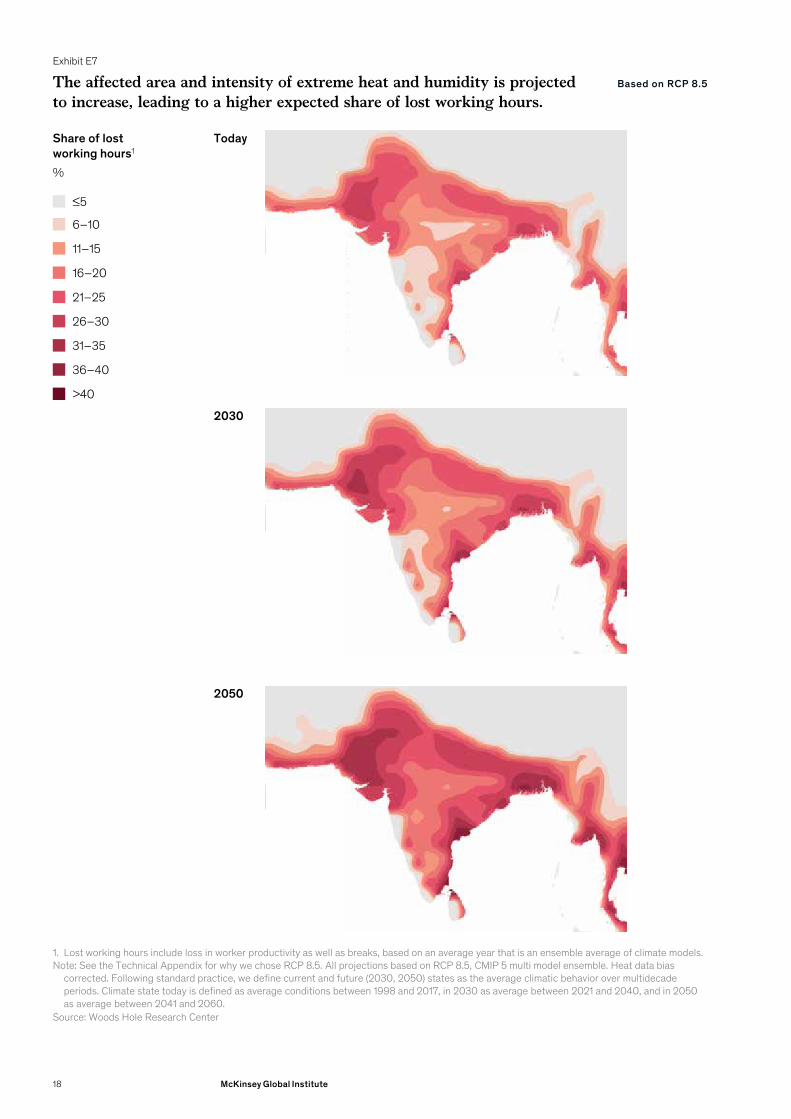
Exhibit E7
The affected area and intensity of extreme heat and humidity is projected to increase, leading to a higher expected share of lost working hours.
Source: Woods Hole Research Center
1. Lost working hours include loss in worker productivity as well as breaks, based on an average year that is an ensemble average of climate models. Note: See the Technical Appendix for why we chose RCP 8.5. All projections based on RCP 8.5, CMIP 5 multi model ensemble. Heat data bias
corrected. Following standard practice, we define current and future (2030, 2050) states as the average climatic behavior over multidecade periods. Climate state today is defined as average conditions between 1998 and 2017, in 2030 as average between 2021 and 2040, and in 2050 as average between 2041 and 2060.
Today
2030
2050
Share of lost working hours1
%
6–10
11–15
16–20
21–25
26–30
31–35
36–40
≤5
>40
Based on RCP 8.5
18 McKinsey Global Institute

Economic and financial systems have similarly been designed and optimized for a certain level of risk and increasing hazards may mean that such systems are vulnerable. We have already noted that supply chains are often designed for efficiency over resiliency, by concentrating production in certain locations and maintaining low inventory levels. Food production is also heavily concentrated; just five regional “breadbasket” areas account for about 60 percent of global grain production. Rising climate hazards might therefore cause such systems to fail, for example if key production hubs are affected. Finance and insurance have vulnerabilities, too; while they were designed to manage for some level of risk, intensifying climate hazards could stretch their limits. For example, consider the residential real estate market in Florida (Exhibit E8). Home owners rely on insurance to build financial resilience against risks like floods, but premiums could rise in the face of increasing risk and insurance does not cover devaluations of home prices. Lenders may bear some risk if home owners default. Among other possible repercussions, federal governments have been acting as backstops but may need to be prepared to finance more.
Other cases we examined highlight large knock-on impacts when thresholds are breached. These come about in particular when the people and assets affected are central to local economies and those local economies are tied into other economic and financial systems.
Ho Chi Minh City, a city prone to monsoonal and storm surge flooding, is one example. We estimate that direct infrastructure asset damage from a 100-year flood today would be on the order of $200 million to $300 million. This could rise to $500 million to $1 billion in 2050, assuming no additional adaptation investment and not including real estate–related impacts. Beyond this direct damage, we estimate that the knock-on costs could be substantial. They would rise from $100 million to $400 million today to between $1.5 billion and as much as $8.5 billion in 2050. We estimate that at least $20 billion of new infrastructure assets are currently planned for construction by 2050, more than doubling the number of major assets in Ho Chi Minh City (Exhibit E9). Many of these new infrastructure assets, particularly the local metro system, have been designed to tolerate an increase in flooding. However, in a worst-case scenario such as a sea-level rise of 180 centimeters, these thresholds could be breached in many locations.25
A further example from our case studies, that of coastal real estate in Florida, shows how climate hazards could have unpredictable financial impacts. The geography of Florida, with its expansive coastline, low elevation, and porous limestone foundation, makes it vulnerable to flooding. Absent any adaptation response, direct physical damages to real estate could grow with the changing climate. Average annual losses for residential real estate due to storm surge from hurricanes amount to $2 billion today. This is projected to increase to about $3 billion to $4.5 billion by 2050, depending on whether exposure is constant or increasing.26 For a tail 100-year hurricane event, storm surge damages could rise from $35 billion today to between $50 billion and $75 billion by 2050.
25 This scenario is extreme, and the probability of it occurring by 2050 is negligible. Nonetheless, it illustrates that infrastructure planned for completion in or shortly before 2050 could experience another step change in risk at some point in 2060 or beyond if significant mitigation does not take place.
26 Analysis conducted by KatRisk; direct average annual losses to all residential real estate (insured and uninsured properties). This is the long-term average loss expected in any one year, calculated by modeling the probability of a climate hazard occurring multiplied by the damage should that hazard occur, and summing over events of all probabilities. Analyses based on sea level rise in line with the US Army Corps of Engineers high curve, one of the recommended curves from the Southeast Florida Regional Climate Change Compact. Southeast Florida Regional Climate Change Compact Sea Level Rise Work Group, Unified sea level rise projection: Southeast Florida, October 2015. More broadly, considering the hurricane hazard, while total hurricane frequency is expected to remain unchanged or to decrease slightly as the climate changes, cumulative hurricane rainfall rates, average intensity, and proportion of storms that reach Category 4–5 intensity are projected to increase, even for a 2°C or less increase in global average temperatures. Thomas Knutson et al., Tropical cyclones and climate change assessment: Part II. Projected response to anthropogenic warming, American Meteorological Society, 2019. Range based on assessing how exposure varies; from constant exposure to exposure based on historical rates of growth of real estate.
19Climate risk and response: Physical hazards and socioeconomic impacts
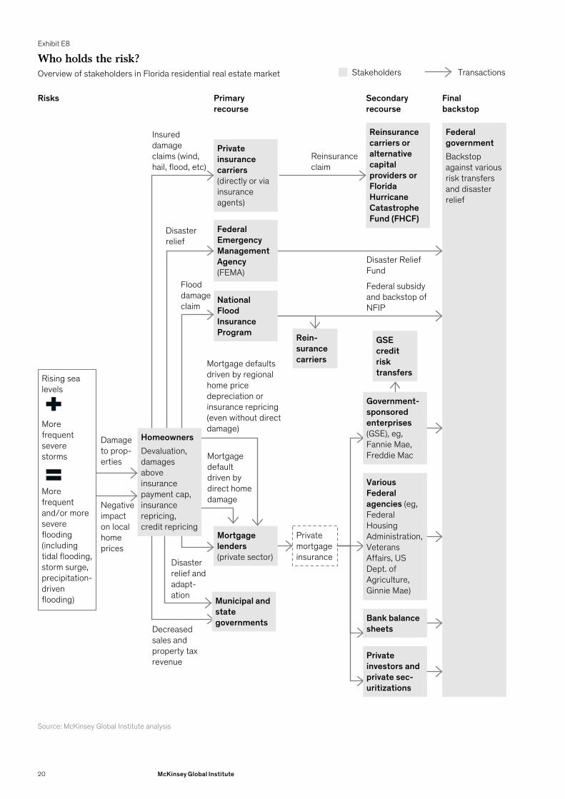
Exhibit E8
Overview of stakeholders in Florida residential real estate marketWho holds the risk?
Source: McKinsey Global Institute analysis
Rein-surancecarriers
TransactionsStakeholders
Private mortgage insurance
Primary recourse
Insured damage claims (wind, hail, flood, etc)
Reinsurance claim
Disaster relief
Disaster Relief Fund
Flood damage claim
Federal subsidy and backstop of NFIP
Mortgage default driven by direct home damage
Mortgage defaults driven by regional home price depreciation or insurance repricing (even without direct damage)
Disaster relief and adapt-ation
Decreased sales and property tax revenue
Negative impact on local home prices
Damage to prop-erties
Secondary recourse
Final backstop
Risks
Rising sea levels
More frequent severe storms
More frequent and/or more severe flooding (including tidal flooding, storm surge, precipitation-driven flooding)
HomeownersDevaluation, damages above insurance payment cap, insurance repricing, credit repricing
Private insurance carriers (directly or via insurance agents)
Federal Emergency Management Agency (FEMA)
National Flood Insurance Program
Mortgage lenders (private sector)
Municipal and state governments
Reinsurance carriers or alternative capital providers or Florida Hurricane Catastrophe Fund (FHCF)
Government-sponsored enterprises(GSE), eg, Fannie Mae, Freddie Mac
Various Federal agencies (eg, Federal Housing Administration, Veterans Affairs, US Dept. of Agriculture, Ginnie Mae)
Bank balance sheets
Private investors and private sec-uritizations
GSE credit risk transfers
Federal governmentBackstop against various risk transfers and disaster relief
20 McKinsey Global Institute
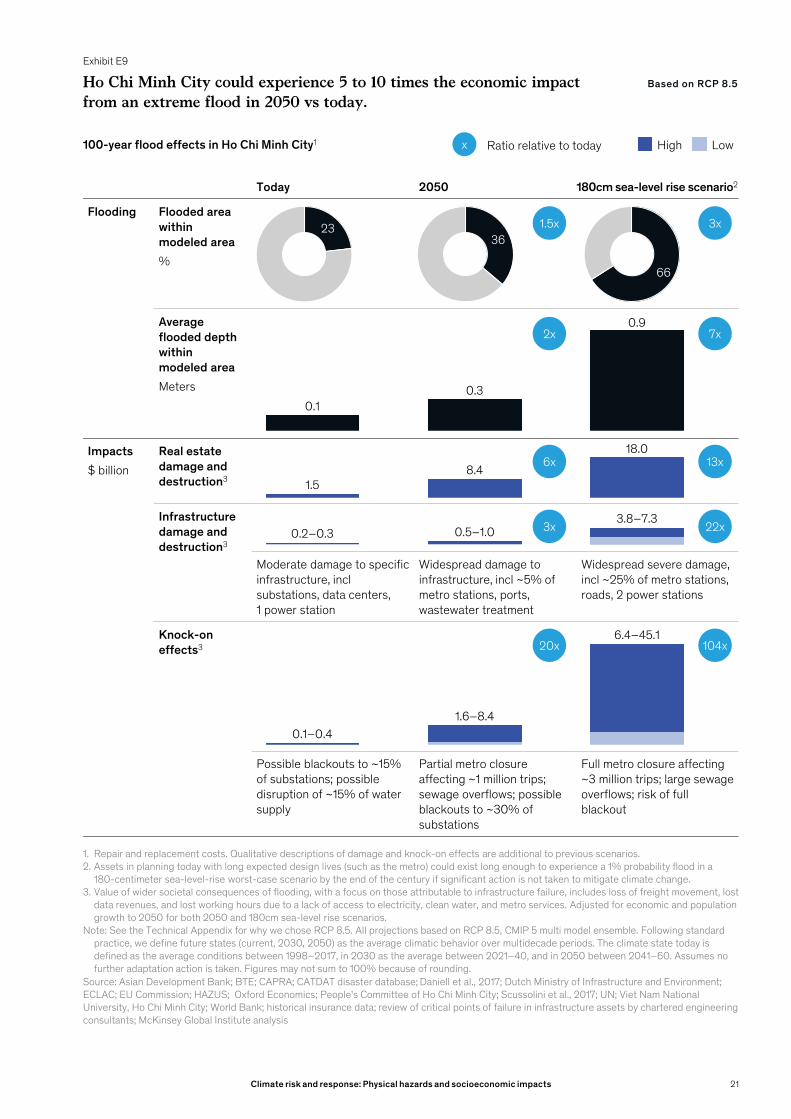
Exhibit E9
Today 2050 180cm sea-level rise scenario2
Flooding Flooded area within modeled area%
Average flooded depth within modeled areaMeters
Impacts$ billion
Real estate damage and destruction3
Infrastructure damage and destruction3
Moderate damage to specific infrastructure, incl substations, data centers, 1 power station
Widespread damage to infrastructure, incl ~5% of metro stations, ports, wastewater treatment
Widespread severe damage, incl ~25% of metro stations, roads, 2 power stations
Knock-on effects3
Possible blackouts to ~15% of substations; possible disruption of ~15% of water supply
Partial metro closure affecting ~1 million trips; sewage overflows; possible blackouts to ~30% of substations
Full metro closure affecting ~3 million trips; large sewage overflows; risk of full blackout
Ho Chi Minh City could experience 5 to 10 times the economic impact from an extreme flood in 2050 vs today.
Source: Asian Development Bank; BTE; CAPRA; CATDAT disaster database; Daniell et al., 2017; Dutch Ministry of Infrastructure and Environment; ECLAC; EU Commission; HAZUS; Oxford Economics; People's Committee of Ho Chi Minh City; Scussolini et al., 2017; UN; Viet Nam National University, Ho Chi Minh City; World Bank; historical insurance data; review of critical points of failure in infrastructure assets by chartered engineering consultants; McKinsey Global Institute analysis
1. Repair and replacement costs. Qualitative descriptions of damage and knock-on effects are additional to previous scenarios.2. Assets in planning today with long expected design lives (such as the metro) could exist long enough to experience a 1% probability flood in a
180-centimeter sea-level-rise worst-case scenario by the end of the century if significant action is not taken to mitigate climate change.3. Value of wider societal consequences of flooding, with a focus on those attributable to infrastructure failure, includes loss of freight movement, lost
data revenues, and lost working hours due to a lack of access to electricity, clean water, and metro services. Adjusted for economic and population growth to 2050 for both 2050 and 180cm sea-level rise scenarios.
Note: See the Technical Appendix for why we chose RCP 8.5. All projections based on RCP 8.5, CMIP 5 multi model ensemble. Following standard practice, we define future states (current, 2030, 2050) as the average climatic behavior over multidecade periods. The climate state today is defined as the average conditions between 1998–2017, in 2030 as the average between 2021–40, and in 2050 between 2041–60. Assumes no further adaptation action is taken. Figures may not sum to 100% because of rounding.
x Ratio relative to today
23
0.2–0.3 0.5–1.03.8–7.3
0.1–0.41.6–8.4
6.4–45.1
36
0.10.3
0.9
1.58.4
18.0
High Low100-year flood effects in Ho Chi Minh City1
Based on RCP 8.5
1.5x 3x
3x 22x
20x 104x
66
2x 7x
6x 13x
21Climate risk and response: Physical hazards and socioeconomic impacts

These numbers do not include the potential devaluation of flooding affected real estate. Exposed homes could see a devaluation of $30 billion to $80 billion, or about 15 to 35 percent, by 2050, all else being equal.27 Lower real estate prices could in turn have knock-on effects, including forgone property tax revenue (a major source of state income), reduced wealth and spending by home owners, reduced, halted, or reversed resident inflow, and forced changes in government spending. For example, rough estimates suggest that the price effects discussed above could impact property tax revenue in some of the most affected counties by about 15 to 30 percent (though impacts across the state could be less, at about 2 to 5 percent). Business activity could be negatively affected, as could the availability and/or price of insurance and mortgage financing in high-risk counties. Financial markets could bring these risks forward, and the recognition of large future changes could lead to price adjustments. Awareness of climate risk could make long-duration borrowing more expensive or unavailable and reduce valuations, for example. This recognition could happen quickly, with the possibility of cascading consequences.
Climate change could create inequality—simultaneously benefiting some regions while hurting others. For example, rising temperatures may boost tourism in areas of northern Europe while reducing the economic vitality of southern European resorts. The volume of water in basins in northern Africa, Greece, and Spain could decline by more than 15 percent by 2050 even as volume in basins in Germany and the Netherlands increases by between 1 and 5 percent.28 The mild Mediterranean climate is expected to grow hotter—by 2050, the climate in the French port city of Marseille could more closely resemble that of Algiers today—which could disrupt key sectors such as tourism and agriculture.29
Within regions, the poorest communities and populations within each of our cases typically are the most vulnerable to climate events. They often lack financial means. For example, acute climate events could trigger harvest failure in multiple breadbasket locations—that is, significantly lower-than-average yields in two or more key production regions for rice, wheat, corn, and soy. We estimate that the chance of a greater than 15 percent yield shock at least once in the decade centered on 2030 could rise from 10 percent today to 18 percent, while the chance of a greater than 10 percent yield shock occurring at least once could rise from 46 to 69 percent.30 Given current high grain stocks, totaling about 30 percent of consumption, the world would not run out of grain. However, historical precedent suggests that prices could spike by 100 percent or more in the short term, in the event of a greater than 15 percent decline in global supply that reduces stocks. This would particularly hurt the poorest communities, including the 750 million people living below the international poverty line.
The global socioeconomic impacts of climate change could be substantial as a changing climate directly affects human, physical, and natural capitalWhile our case studies illustrate the localized impacts of a changing climate, rising temperatures are a global trend. To understand how physical climate hazards could evolve around the world, we developed a global geospatial assessment of climate impacts over the next 30 years covering 105 countries.31 We again rely on our framework of the direct impacts of climate change on five human, physical, and natural systems. For each system we have identified one or more measures
27 Analysis supported by First Street Foundation, 2019. Ranges based on whether homes that frequently flood (>50x per year), see more significant devaluations or not. Note that other factors could also affect the prices of homes and that has not been factored in. Much of the literature finds that, at least historically, prices of exposed properties have risen slower than prices of unexposed properties, rather than declined in absolute terms. For further details, see the Florida case study.
28 World Resources Institute Water Risk Atlas, 2018.29 Jean-Francois Bastin et al., Understanding climate change from a global analysis of city analogues. PLoS ONE 14(7):
e0217592, 2019.30 To estimate the likelihood, we employ crop models from the AgMIP model library that translate outputs from climate models
into crop yields for each modeled grid cell. Using all available climate models over a period of 20 years, we construct a probability distribution of yields for each crop in each grid cell. Note that we are taking into account potentially positive effects on plant growth from higher CO2 levels (“CO2 fertilization”). Analysis is based on an assumption of no improvements in agricultural productivity (consistent with our “inherent risk” framing). See breadbasket case for further details.
31 To conduct this analysis, we have relied on geospatial climate hazard data, including from Woods Hole Research Center analysis of CMIP5 Global Climate Model output, the World Resources Institute, the European Center for Medium-Range Weather Forecasts and data from Rubel et al. (obtained from the National Oceanic and Atmospheric Administration). We used geospatial data on population, capital stock, and GDP from the European Commission Global Human Settlement (GHS) and the UN Global Assessment Report on Disaster Risk Reduction, as well as data from other sources as described in Chapter 4. Notably, we have focused our analysis on a subset of possible climate hazards: lethal heat waves, heat and humidity and its impact on workability, water stress, riverine flooding, drought, and the impact of increased temperature and changes in precipitation on biome shifts. Analysis based on an RCP 8.5 scenario.
22 McKinsey Global Institute
to define the impact of climate change, often building on the risk measures used in our case studies, and choosing the best possible measures based on broad country coverage and data availability.32 For example, for livability and workability, we use the measures of the share of population living in areas projected to experience a non-zero annual probability of lethal heat waves as well as the annual share of effective outdoor working hours affected by extreme heat and humidity in climate-exposed regions. This is similar to the approach followed in our India case study.
We find that all 105 countries are expected to experience an increase in at least one major type of impact on their stock of human, physical, and natural capital by 2030. Intensifying climate hazards could put millions of lives at risk, as well as trillions of dollars of economic activity and physical capital, and the world’s stock of natural capital. The intensification of climate hazards across regions will bring areas hitherto unexposed to impacts into new risk territory.
— Livability and workability. By 2030, under an RCP 8.5 scenario, our research suggests that between 250 million and 360 million people could live in regions where there is a non-zero probability of a heat wave exceeding the threshold for survivability for a healthy human being in the shade (a measure of livability, without factoring in air conditioner penetration).33 The average probability of a person living in an at-risk region experiencing such a lethal heat wave at least once over the decade centered on 2030 is estimated to be approximately 60 percent.34 Some exposed regions will have a lower probability, and some regions higher. By 2050, the number of people living in regions exposed to such heat waves could rise further, to between 700 million and 1.2 billion, again without factoring in an adaptation response via air conditioner penetration. This reflects the fact that some of the most heavily populated areas of the world are usually also the hottest and most humid, and, as described below, these areas are becoming even hotter and more humid. Today, air conditioner penetration is roughly 10 percent across India, and roughly 60 percent across China.35 The global average number of working hours that could be lost due to increasing heat and humidity in exposed regions (a measure of workability impacts) could almost double by 2050, from 10 percent to 15 to 20 percent. This is because more regions of the world are exposed, and the ones that are exposed would see higher intensity of heat and humidity effects. We used these projections to estimate the resulting GDP at risk from lost working hours. This could amount to $4 trillion to $6 trillion globally at risk by 2050 in an average year (Exhibit E10). This the equivalent of 2 to 3.5 percent of 2050 GDP, up from about 1.5 percent today.36
32 The indicators used in our geospatial analysis include: share of population that lives in areas experiencing a non-zero annual probability of lethal heat waves, annual share of effective outdoor working hours affected by extreme heat and humidity in climate exposed-regions, water stress as measured by the annual demand of water as a share of annual supply of water (these three are measures of livability and workability, and are considered in our India case and Mediterranean cases), annual share of capital stock at risk of flood damage in climate-exposed regions (asset destruction and infrastructure services; similar measures of capital stock damage are used in our Florida and Inundation cases), share of time spent in drought over a decade (measure of food systems; we also consider the impact of drought in our Mediterranean case), share of land surface changing climate classification annually (measure of natural capital; this was used for our geospatial analysis to allow us to develop a global measure of natural capital risk). Notably, drought is the one measure of hazard rather than risk used in this framework. This was done because of data limitations with obtaining data on impacts on agricultural yield by country, since the AgMIP climate models used to project agricultural yields tend only to be used for relatively large breadbasket regions, rather than at a country level. We are able to use the AgMIP results to provide global trends on breadbaskets and results pertaining to large breadbasket regions; however, such results were not included in the country-by-country analysis. We also excluded risk due to hazards like hurricanes, storm surge, and forest fires due to challenges obtaining sufficiently granular and robust data across countries. See Chapter 4 for details.
33 Here, as before, lethal heat wave refers to a three-day period with average daily maximum wet-bulb temperatures exceeding 34 degrees Celsius. This temperature was chosen because urban areas with a high urban heat island effect could amplify 34°C ambient temperatures over the 35°C wet-bulb survivability threshold. These numbers are subject to uncertainty related to the future behavior of atmospheric aerosols and urban heat island or cool island effects. If a non-zero probability of lethal heat waves in certain regions occurred in the models for today, this was set to zero to account for the poor representation of the high levels of observed atmospheric aerosols in those regions in the CMIP5 models. High levels of atmospheric aerosols provide a cooling effect that masks the risk. See India case for further details. This analysis excludes grid-cells where the the likelihood of lethal heat waves is <1 percent, to eliminate areas of low statistical significance. Additionally, these numbers assume no air-conditioning protection, and as such should be considered an upper bound. See Chapter 2 for details. Analysis based on an RCP 8.5 scenario.
34 This calculation is a rough approximation. It assumes that the annual probability of roughly 9 percent applies to every year in the decade centered around 2030. We first calculate the cumulative probability of a heat wave not occurring in that decade, which is 91 percent raised to the power of 10. The cumulative probability of a heat wave occurring at least once in the decade is then 1 minus that number.
35 India Cooling Action Plan Draft, Ministry of Environment, Forest & Climate Change, Government of India, September 2018; The Future of Cooling in China, IEA, Paris, 2019.
36 The range here is based on the pace of sectoral transition across countries. GDP at risk will be higher if a greater portion of the economy is occupied in outdoor work. The lower end of the range assumes that today’s sectoral composition persists, while the higher end is based on projections from IHS Markit Economics and Country Risk on sectoral transitions.
23Climate risk and response: Physical hazards and socioeconomic impacts

Exhibit E10
GDP at risk from the effect of extreme heat and humidity on effective working hours is expected to increase over time.
Source: IHS Markit Economics and Country Risk; Woods Hole Research Center; McKinsey Global Institute analysis
Note: See the Technical Appendix for why we chose RCP 8.5. All projections based on RCP 8.5, CMIP 5 multi model ensemble. Heat data bias corrected. These maps do not consider sectoral shifts when projecting impact on labor productivity into the future—the percentage and spatial distribution of outdoor labor are held constant. For this analysis, outdoor labor is considered to include agriculture, construction, and mining and quarrying only, and knock-on impacts on other sectors are not considered. Following standard practice, we define current and future (2030, 2050) states as the average climatic behavior over multidecade periods. Climate state today is defined as average conditions between 1998 and 2017, in 2030 as average between 2021 and 2040, and in 2050 as average between 2041 and 2060.
GDP at risk from working hours impacted by heat and humidity (direct effect only, scenario of no sectoral transitions)%
≤0.1
0.2–1.0
1.1–5.0
5.1–10.0
10.1–15.0
15.1–20.0
>20
Today
2030
2050
Based on RCP 8.5
24 McKinsey Global Institute
— Food systems. Our research suggests an increase in global agricultural yield volatility that skews toward worse outcomes. For example, by 2050, the annual probability of a greater than 10 percent reduction in yields for wheat, corn, soy, and rice in a given year is projected to increase from 6 to 18 percent.37 The annual probability of a greater than 10 percent increase in yield in a given year is expected to rise from 1 percent to 6 percent. These trends are not uniform across countries and, importantly, some could see improved agricultural yields, while others could suffer negative impacts. For example, the average breadbasket region of Europe and Russia is expected to experience a 4 percent increase in average yields by 2050. While the annual probability of a greater than 10 percent yield failure there will increase, from 8 percent to 11 percent annually by 2050, the annual probability of a bumper year with a greater than 10 percent higher-than-average yield in the same period will increase by more, from 8 percent to 18 percent.
— Physical assets and infrastructure services. Assets can be destroyed or services from infrastructure assets disrupted from a variety of hazards, including flooding, forest fires, hurricanes, and heat. Statistically expected damage to capital stock from riverine flooding could double by 2030 from today’s levels and quadruple by 2050. Data availability has made it challenging to develop similar estimates for the much larger range of impacts from tidal flooding, fires, and storms.38
— Natural capital. With temperature increases and precipitation changes, the biome in parts of the world is expected to shift. The biome refers to the naturally occurring community of flora and fauna inhabiting a particular region. For this report, we have used changes in the Köppen Climate Classification System as an indicative proxy for shifts in biome.39 For example, tropical rainforests exist in a particular climatic envelope that is defined by temperature and precipitation characteristics. In many parts of the world, this envelope could begin to be displaced by a much drier “tropical Savannah” climate regime that threatens tropical rainforests. Today, about 25 percent of the Earth’s land area has already experienced a shift in climate classification compared with the 1901–25 period. By 2050, that number is projected to increase to about 45 percent. Almost every country will see some risk of biome shift by 2050, affecting ecosystem services, local livelihoods, and species’ habitat.
Countries with the lowest per capita GDP levels are generally more exposedWhile all countries are affected by climate change, our research suggests that the poorest countries are generally more exposed, as they often have climates closer to dangerous physical thresholds. The patterns of this risk increase look different across countries. Broadly speaking, countries can be divided into six groups based on their patterns of increasing risk (Exhibits E11, E12, and E13).40
37 Global yields based on an analysis of six global breadbaskets that make up 70 percent of global production of four crops; wheat, soy, maize, and rice. Cumulative likelihood calculated for the decade centered on 2030 and 2050 by using annual probabilities for the climate state in the 2030 period, and the 2050 period respectively. Annual probabilities are independent and can therefore be aggregated to arrive at a cumulative decadal probability. Yield anomalies here are measured relative to the 1998-2017 average yield.
38 See Chapter 4 for details.39 The Köppen climate system divides climates into five main climate groups with each group further subdivided based on
seasonal precipitation and temperature patterns. This is not a perfect system for assessing the location and composition of biomes; however, these two characteristics do correlate very closely with climate classification, and therefore this was assessed as a reasonable proxy for risk of disruptive biome changes.
40 These patterns were primarily based on looking at indicators relating to livability and workability, food systems, and natural capital. The annual share of capital stock at risk of riverine flood damage in climate-exposed regions indicator was considered but was not found to be the defining feature of any country grouping aside from a lower-risk group of countries.
25Climate risk and response: Physical hazards and socioeconomic impacts

Exhibit E11
We identify six types of countries based on their patterns of expected change in climate impacts.
Source: Woods Hole Research Center; World Resources Institute Water Risk Atlas, 2018; World Resources Institute Aqueduct Global Flood Analyzer; Rubel and Kottek, 2010; McKinsey Global Institute analysis
1. We define a lethal heat wave as a 3-day period with maximum daily wet-bulb temperatures exceeding 34°C wet-bulb. This threshold was chosen because the commonly defined heat threshold for human survivability is 35°C wet-bulb, and large cities with significant urban heat island effects could push 34°C wet-bulb heat waves over the 35°C threshold. These projections are subject to uncertainty related to the future behavior of atmospheric aerosols and urban heat island or cooling island effects.
2. Water stress is measured as annual demand of water as a share of annual supply of water. For this analysis, we assume that the demand for water stays constant over time, to allow us to measure the impact of climate change alone. Water stress projections for arid, low-precipitation regions were excluded due to concerns about projection robustness.
3. Risk values are calculated based on “expected values”, ie, probability-weighted value at risk.Note: See the Technical Appendix for why we chose RCP 8.5. All projections based on RCP 8.5, CMIP 5 multi model ensemble. Heat data bias
corrected. Following standard practice, we define current and future (2030, 2050) states as the average climatic behavior over multidecade periods. Climate state today is defined as average conditions between 1998 and 2017, in 2030 as average between 2021 and 2040, and in 2050 as average between 2041 and 2060.
Risk decrease No or slight risk increase Moderate risk increase High risk increase
Based on RCP 8.5
Chan
ge in
… (2
018–
50, p
p)Livability and workability
Food systems
Physical assets/infrastructure services
Natural capital
Country
Share of population that
lives in areas experiencing a non-zero
annual prob-ability of lethal
heat waves1
Annual share of effective
outdoor working hours
affected by extreme heat and humidity
in climate exposed-regions
Waterstress2
Share of time spent in
drought over a decade
Annual share of capital stock
at risk of riverine flood
damage in climate-exposed regions3
Share of land surface
changing climate
classificationSignificantly hotter and more humid countriesBangladeshIndiaNigeriaPakistanOther countries in group: Benin, Burkina Faso, Cambodia, Cote d'Ivoire, Eritrea, Ghana, Myanmar, Niger, Senegal, Thailand, Vietnam, YemenAverage(all countries in group)Hotter and more humid countriesEthiopiaIndonesiaJapanPhilippinesOther countries in group: Angola, Cameroon, Chad, Ecuador, Guinea, Guyana, Jordan, Laos, Liberia, Madagascar, Papua New Guinea, Saudi Arabia, Somalia, Suriname, Tanzania, Uganda, Uruguay, ZambiaAverage(all countries in group)Hotter countriesColombiaDem. Rep. Congo
26 McKinsey Global Institute

Exhibit E12
We identify six types of countries based on their patterns of expected change in climate impacts (continued).
Source: Woods Hole Research Center; World Resources Institute Water Risk Atlas, 2018; World Resources Institute Aqueduct Global Flood Analyzer; Rubel and Kottek, 2010; McKinsey Global Institute analysis
1. We define a lethal heat wave as a 3-day period with maximum daily wet-bulb temperatures exceeding 34°C wet-bulb. This threshold was chosen because the commonly defined heat threshold for human survivability is 35°C wet-bulb, and large cities with significant urban heat island effects could push 34°C wet-bulb heat waves over the 35°C threshold. These projections are subject to uncertainty related to the future behavior of atmospheric aerosols and urban heat island or cooling island effects.
2. Water stress is measured as annual demand of water as a share of annual supply of water. For this analysis, we assume that the demand for water stays constant over time, to allow us to measure the impact of climate change alone. Water stress projections for arid, low-precipitation regions were excluded due to concerns about projection robustness.
3. Risk values are calculated based on “expected values”, ie, probability-weighted value at risk.Note: See the Technical Appendix for why we chose RCP 8.5. All projections based on RCP 8.5, CMIP 5 multi model ensemble. Heat data bias
corrected. Following standard practice, we define current and future (2030, 2050) states as the average climatic behavior over multidecade periods. Climate state today is defined as average conditions between 1998 and 2017, in 2030 as average between 2021 and 2040, and in 2050 as average between 2041 and 2060.
Based on RCP 8.5
Chan
ge in
… (2
018–
50, p
p)Livability and workability
Food systems
Physical assets/infrastructure services
Natural capital
Country
Share of population that
lives in areas experiencing a non-zero
annual prob-ability of lethal
heat waves1
Annual share of effective
outdoor working hours
affected by extreme heat and humidity
in climate exposed-regions
Waterstress2
Share of time spent in
drought over a decade
Annual share of capital stock
at risk of riverine flood
damage in climate-exposed regions3
Share of land surface
changing climate
classificationHotter countries (continued)MalaysiaSouth KoreaOther countries in group: Botswana, Central African Rep., Cuba, Gabon, Guatemala, Honduras, Hungary, Libya, Malawi, Mali, Mauritania, Mozambique, Namibia, Nicaragua, Oman, Paraguay, Rep. Congo, Romania, Serbia, Venezuela, ZimbabweAverage(all countries in group)Increased water stress countriesEgyptIranMexicoTurkeyOther countries in group: Algeria, Australia, Azerbaijan, Bulgaria, Greece, Italy, Kazakhstan, Kyrgyzstan, Morocco, Portugal, South Africa, Spain, Syria, Tajikistan, Tunisia, Turkmenistan, Ukraine, UzbekistanAverage(all countries in group)Lower-risk countriesFranceGermany
Risk decrease No or slight risk increase Moderate risk increase High risk increase
27Climate risk and response: Physical hazards and socioeconomic impacts
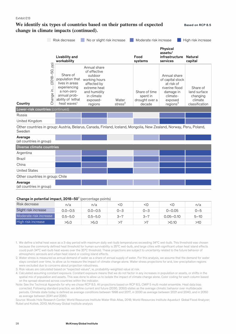
Exhibit E13
We identify six types of countries based on their patterns of expected change in climate impacts (continued).
Source: Woods Hole Research Center; World Resources Institute Water Risk Atlas, 2018; World Resources Institute Aqueduct Global Flood Analyzer; Rubel and Kottek, 2010; McKinsey Global Institute analysis
1. We define a lethal heat wave as a 3-day period with maximum daily wet-bulb temperatures exceeding 34°C wet-bulb. This threshold was chosen because the commonly defined heat threshold for human survivability is 35°C wet-bulb, and large cities with significant urban heat island effects could push 34°C wet-bulb heat waves over the 35°C threshold. These projections are subject to uncertainty related to the future behavior of atmospheric aerosols and urban heat island or cooling island effects.
2. Water stress is measured as annual demand of water as a share of annual supply of water. For this analysis, we assume that the demand for water stays constant over time, to allow us to measure the impact of climate change alone. Water stress projections for arid, low-precipitation regions were excluded due to concerns about projection robustness.
3. Risk values are calculated based on “expected values”, ie, probability-weighted value at risk.4. Calculated assuming constant exposure. Constant exposure means that we do not factor in any increases in population or assets, or shifts in the
spatial mix of population and assets. This was done to allow us to isolate the impact of climate change alone. Color coding for each column based on the spread observed across countries within the indicator.
Note: See the Technical Appendix for why we chose RCP 8.5. All projections based on RCP 8.5, CMIP 5 multi model ensemble. Heat data bias corrected. Following standard practice, we define current and future (2030, 2050) states as the average climatic behavior over multidecade periods. Climate state today is defined as average conditions between 1998 and 2017, in 2030 as average between 2021 and 2040, and in 2050 as average between 2041 and 2060.
Based on RCP 8.5
Chan
ge in
… (2
018–
50, p
p)Livability and workability
Food systems
Physical assets/infrastructure services
Natural capital
Country
Share of population that
lives in areas experiencing a non-zero
annual prob-ability of lethal
heat waves1
Annual share of effective
outdoor working hours
affected by extreme heat and humidity
in climate exposed-regions
Waterstress2
Share of time spent in
drought over a decade
Annual share of capital stock
at risk of riverine flood
damage in climate-exposed regions3
Share of land surface
changing climate
classificationLower-risk countries (continued)RussiaUnited KingdomOther countries in group: Austria, Belarus, Canada, Finland, Iceland, Mongolia, New Zealand, Norway, Peru, Poland, SwedenAverage(all countries in group)Diverse climate countriesArgentinaBrazilChinaUnited StatesOther countries in group: ChileAverage(all countries in group)
Change in potential impact, 2018–504 (percentage points)Risk decrease n/a n/a <0 <0 <0 n/aSlight risk increase 0.0–0.5 0.0–0.5 0–3 0–3 0–0.05 0–5Moderate risk increase 0.5–5.0 0.5–5.0 3–7 3–7 0.05–0.10 5–10High risk increase >5.0 >5.0 >7 >7 >0.10 >10
Risk decrease No or slight risk increase Moderate risk increase High risk increase
28 McKinsey Global Institute

— Significantly hotter and more humid countries. Hot and humid countries such as India and Pakistan are expected to become significantly hotter and more humid by 2050. Countries in this group are near the equator in Africa, Asia, and the Persian Gulf. They are characterized by extreme increases in heat and humidity impacts on workability, as well as a decrease in water stress. The potential livability impact that countries in this group face is projected to increase, because of the combination of heat and humidity.
— Hotter and more humid countries. This group includes the Philippines, Ethiopia, and Indonesia. These countries are typically between the equator and the 30-degree north and 30-degree south lines of latitude. They face a large potential increase in heat and humidity impacts on workability but may not become so hot or humid that they exceed livability thresholds. Water stress is also expected to decrease for these countries.
— Hotter countries. This group includes Colombia, the Democratic Republic of Congo, and Malaysia. Many countries in this group are near the equator. They are characterized by a large increase in heat and humidity impact on workability but are not expected to become so hot or humid that they pass livability thresholds. This group of countries is not expected to become wetter, and some of these countries could even become substantially drier and see increased water stress.
— Increased water stress countries. This group includes Egypt, Iran, and Mexico, which intersect the 30-degree north or south line of latitude. They are characterized by a large increase in water stress and drought frequency, and among the largest increases in biome change. In these locations, Hadley cells (the phenomenon responsible for the atmospheric transport of moisture from the tropics, and therefore location of the world’s deserts) are expanding, and these countries face a projected reduction in rainfall.
— Lower-risk increase countries. This group includes Germany, Russia, and the United Kingdom. Many countries in this group lie outside the 30-degree north and south lines of latitude and are generally cold countries. Some are expected to see a decrease in overall impact on many indicators. These countries are characterized by very low levels of heat and humidity impacts and many countries are expected to see decreases in water stress and time spent in drought. As these countries grow warmer, they will likely see the largest increase in biome change as the polar and boreal climates retreat poleward and disappear. The share of capital stock at risk of riverine flood damage in climate-exposed regions could also potentially increase in some of these countries.
— Diverse climate countries. The final group consists of countries that span a large range of latitudes and therefore are climatically heterogeneous. Examples include Argentina, Brazil, Chile, China, and the United States.41 While average numbers may indicate small risk increases, these numbers mask wide regional variations. The United States, for example, has a hot and humid tropical climate in the Southeast, which will see dramatic increases in heat risk to outdoor work but is not projected to struggle with water scarcity. The West Coast region, however, will not see a big increase in heat risk to outdoor work, but will struggle with water scarcity and drought. In Alaska, the primary risk will be the shifting boreal biome and the attendant ecosystem disruptions.
The risk associated with the impact on workability from rising heat and humidity is one example of how poorer countries could be more vulnerable to climate hazards (Exhibit E14).
41 To some extent, many countries could experience diversity of risk within their boundaries. Here we have focused on highlighting countries with large climatic variations, and longitudinal expanse, which drives different outcomes in different parts of the country.
29Climate risk and response: Physical hazards and socioeconomic impacts

Exhibit E14
Countries with the lowest per capita GDP levels face the biggest increase in risk for some indicators.
Source: Woods Hole Research Center; Rubel and Kottek, 2010; IMF; World Bank; UN; McKinsey Global Institute analysis
Change, 2018–50Percentage points
Annual share of effective outdoor working hours affected by extreme heat and humidity in climate-exposed regionsCorrelation coefficient:r = -0.49
Share of land surface changing climate classificationCorrelation coefficient:r = 0.35
10
100,0001,000100 10,000
8
6
4
0
2
12
14
16
18
China
India
UnitedStates
Indonesia
Brazil
20
10,000100 1,000 100,0000
10
30
40
50
60
70
80
90
100
GDP per capita, 2017 (current $)Log scale
India
ChinaUnitedStates
France
Africa Americas Europe andCentral Asia
Asia and the Pacific
Arab states
Note: Not to scale. See the Technical Appendix for why we chose RCP 8.5. All projections based on RCP 8.5, CMIP 5 multi model ensemble. Heat data bias corrected. Following standard practice, we define current and future (2030, 2050) states as the average climatic behavior over multidecade periods. Climate state today is defined as average conditions between 1998 and 2017, in 2030 as average between 2021 and 2040, and in 2050 as average between 2041 and 2060.
Based on RCP 8.5
30 McKinsey Global Institute
When looking at the workability indicator (that is, the share of outdoor working hours lost to extreme heat and humidity), the top quartile of countries (based on GDP per capita) have an average increase in risk by 2050 of approximately one to three percentage points, whereas the bottom quartile faces an average increase in risk of about five to ten percentage points. Lethal heat waves show less of a correlation with per capita GDP, but it is important to note that several of the most affected countries—Bangladesh, India, and Pakistan, to name a few—have relatively low per capita GDP levels.
Conversely, biome shift is expected to affect northern and southern latitude countries. Since many of these countries have higher per capita GDP levels, this indicator shows a positive correlation with development levels.
Leaders will need to better understand the impacts of physical climate risk, while accelerating adaptation and mitigation In the face of these challenges, policy makers and business leaders will need to put in place the right tools, analytics, processes, and governance to properly assess climate risk, adapt to risk that is locked in, and decarbonize to reduce the further buildup of risk. In Box E3 that concludes this summary, we present a range of questions that stakeholders could consider as they look to manage risk.
Integrating climate risk into decision makingMuch as thinking about information systems and cyber-risks has become integrated into corporate and public-sector decision making, climate change will also need to feature as a major factor in decisions. For companies, this will mean taking climate considerations into account when looking at capital allocation, development of products or services, and supply chain management, among others. For cities, a climate focus will become essential for urban planning decisions. Financial institutions could consider the risk in their portfolios.42 Moreover, while this report has focused on physical risk, a comprehensive risk management strategy will also need to include an assessment of transition and liability risk, and the interplay between these forms of risk.
Developing a robust quantitative understanding is complex, for the many reasons outlined in this report. It requires the use of new tools, metrics, and analytics. Companies and communities are beginning to assess their exposure to climate risk, but much more needs to be done. Lack of understanding significantly increases risks and potential impacts across financial markets and socioeconomic systems, for example, by driving capital flows to risky assets in risky geographies or increasing the likelihood of stakeholders being caught unprepared.
At the same time, opportunities from a changing climate will emerge and require consideration. These could arise from a change in the physical environment, such as new places for agricultural production, or for sectors like tourism, as well as through the use of new technologies and approaches to manage risk in a changing climate.
One of the biggest challenges could stem from using the wrong models to quantify risk. These range from financial models used to make capital allocation decisions to engineering models used to design structures. As we have discussed, there is uncertainty associated with global and regional climate models, underlying assumptions on emissions paths, and, most importantly, in translating climate hazards to potential physical and financial damages. While these uncertainties are non-negligible, continued reliance on current models based on stable historical climate and economic data presents an even higher “model risk.”
42 See, for example, Getting physical: Scenario analysis for assessing climate-related risks, Blackrock Investment Institute, April 2019.
31Climate risk and response: Physical hazards and socioeconomic impacts
Three examples of how models could be inappropriate for the changing climate are as follows:
— Geography. Current models may not sufficiently take into account geospatial dimensions. As this report highlights, direct impacts of climate change are local in nature, requiring understanding exposure to risk via geospatial analysis. For example, companies will need to understand how their global asset footprint is exposed to different forms of climate hazard in each of their main locations and indeed in each of the main locations of their critical suppliers.
— Non-stationarity. Given the constantly changing or non-stationary climate, assumptions based on historical precedent and experience will need to be rethought. That could include, for example, how resilient to make new factories, what tolerance levels to employ in new infrastructure, and how to design urban areas. Decisions will need to take into consideration that the climate will continue to change over the next several decades.
— Sample bias. Decision makers often rely on their own experiences as a frame for decisions; in a changing climate, that can result in nonlinear effects and thus lead to incorrect assessments of future risk.
Accelerating the pace and scale of adaptationSocieties have been adapting to the changing climate, but the pace and scale of adaptation will likely need to increase significantly. Key adaptation measures include protecting people and assets, building resilience, reducing exposure, and ensuring that appropriate financing and insurance are in place.
— Protecting people and assets. Measures to protect people and assets to the extent possible can help limit risk. Steps can range from prioritizing emergency response and preparedness to erecting cooling shelters and adjusting working hours for outdoor workers exposed to heat. Hardening existing infrastructure and assets is a key response. According to the UN Environment Programme, the cost of adaptation for developing countries may range from $140 billion to $300 billion a year by 2030. This could rise to $280 billion to $500 billion by 2050.43 Hardening of infrastructure could include both “gray” infrastructure—for example, raising elevation levels of buildings in flood-prone areas—and natural capital or “green” infrastructure. One example of this is the Dutch Room for the River program, which gives rivers more room to manage higher water levels.44 Another example is mangrove plantations, which can provide storm protection.
Factoring decisions about protection into new buildings will likely be more cost-effective than retrofitting.45 For example, infrastructure systems or factories may be designed to withstand what used to be a 1-in-200-year event. With a changing climate, what constitutes such an event may look different, and design parameters will need to be reassessed. Estimates suggest that $30 trillion to $50 trillion will be spent on infrastructure in the next ten years, much of it in developing countries.46 Designing such infrastructure with climate risk in mind may help reduce downstream repair and rebuilding costs. Moreover, infrastructure that specifically helps protect assets and people will be needed, for example cooling technologies including green air-conditioning (high energy efficiency HVAC powered by low carbon power, for example), emergency shelters, and passive urban design.
43 Anne Olhoff et al., The adaptation finance gap report, UNEP DTU Partnership, 2016. 44 See Room for the River, ruimtevoorderivier.nl/english/.45 Michael Della Rocca, Tim McManus, and Chris Toomey, Climate resilience: Asset owners need to get involved now,
McKinsey.com, January 2009.46 Bridging global infrastructure gaps, McKinsey Global Institute, June 2016; Bridging infrastructure gaps: Has the world
made progress? McKinsey Global Institute, October 2017.
32 McKinsey Global Institute
— Building resilience. Asset hardening will need to go hand-in-hand with measures that make systems more resilient and robust in a world of rising climate hazard. Building global inventory to mitigate risks of food and raw material shortages is an example of resilience planning, leveraging times of surplus and low prices. To make the food system more resilient, private and public research could be expanded, for example on technology that aims to make crops more resistant to abiotic and biotic stresses. As noted, climate change challenges key assumptions that have been used to optimize supply chain operations in the past. Those assumptions may thus need to be rethought, for example by building backup inventory levels in supply chains to protect against interrupted production, as well as establishing the means to source from alternate locations and/or suppliers.
— Reducing exposure. In some instances, it may also be necessary to reduce exposure by relocating assets and communities in regions that may be too difficult to protect, that is, to retreat from certain areas or assets. Given the long lifetimes of many physical assets, the full life cycle will need to be considered and reflected in any adaptation strategy. For example, it may make sense to invest in asset hardening for the next decade but also to shorten asset life cycles. In subsequent decades, as climate hazards intensify and the cost-benefit equation of physical resilience measures is no longer attractive, it may become necessary to relocate and redesign asset footprints altogether.
— Insurance and finance. While insurance cannot eliminate the risk from a changing climate, it is a crucial shock absorber to help manage risk.47 Insurance can help provide system resilience to recover more quickly from disasters and reduce knock-on effects. It can also encourage behavioral changes among stakeholders by sending appropriate risk signals—for example, to homeowners buying real estate, lenders providing loans, and real estate investors financing real estate build-out.
Instruments such as parametrized insurance and catastrophe bonds can provide protection against climate events, minimizing financial damage and allowing speedy recovery after disasters. These products may help protect vulnerable populations that could otherwise find it challenging to afford to rebuild after disasters. Insurance can also be a tool to reduce exposure by transferring risk (for example, crop insurance allows transferring the risk of yield failure due to drought) and drive resilience (such as by enabling investments in irrigation and crop-management systems for rural populations who would otherwise be unable to afford this).
However, as the climate changes, insurance might need to be further adapted to continue providing resilience and, in some cases, avoid potentially adding vulnerability to the system. For example, current levels of insurance premiums and levels of capitalization among insurers may well prove insufficient over time for the rising levels of risk; and the entire risk transfer process (from insured to insurer to reinsurer to governments as insurers of last resort) and each constituents’ ability to fulfil their role may need examination. Without changes in risk reduction, risk transfer, and premium financing or subsidies, some risk classes in certain areas may become harder to insure, widening the insurance gap that already exists in some parts of the world without government intervention.
Innovative approaches will also likely be required to help bridge the underinsurance gap. Premiums are already sometimes subsidized—one example is flood insurance, which is often nationally provided and subsidized. Such support programs however might need to be carefully rethought to balance support to vulnerable stakeholders with allowing appropriate risk signals in the context of growing exposure and multiple knock-on effects. One answer might be providing voucher programs to help ensure affordability for vulnerable populations, while maintaining premiums at a level that reflects the appropriate
47 Goetz von Peter, Sebastian von Dahlen, and Sweta Saxena, Unmitigated disasters? New evidence on the macroeconomic cost of natural catastrophes, BIS Working Papers, Number 394, December 2012.
33Climate risk and response: Physical hazards and socioeconomic impacts

risk. Trade-offs between private and public insurance, and for individuals, between when to self-insure or buy insurance, will need to be carefully evaluated. In addition, underwriting may need to shift to drive greater risk reduction in particularly vulnerable areas (for example, new building codes or rules around hours of working outside). This is analogous to fire codes that emerged in cities in order to make buildings insurable. Insurance may also need overcome a duration mismatch; for example, homeowners may expect long-term stability for their insurance premiums, whereas insurers may look to reprice annually in the event of growing hazards and damages. This could also apply to physical supply chains that are currently in place or are planned for the future, as the ability to insure them affordably may become a criterion of growing significance.
Mobilizing finance to fund adaptation measures, particularly in developing countries, is also crucial. This may require public-private partnerships or participation by multilateral institutions, to prevent capital flight from risky areas once climate risk is appropriately recognized. Innovative products and ventures have been developed recently to broaden the reach and effectiveness of these measures. They include “wrapping” a municipal bond into a catastrophe bond, to allow investors to hold municipal debt without worrying about hard-to-assess climate risk. Governments of developing nations are increasingly looking to insurance/reinsurance carriers and other capital markets to improve their resiliency to natural disasters as well as give assurances to institutions that are considering investments in a particular region.
— Addressing tough adaptation choices. Implementing adaptation measures could be challenging for many reasons. The economics of adaptation could worsen in some geographies over time, for example, those exposed to rising sea levels. Adaptation may face technical or other limits. In other instances, there could be hard trade-offs that need to be assessed, including who and what to protect and who and what to relocate. For example, the impact on individual home owners and communities needs to be weighed against the rising burden of repair costs and post-disaster aid, which affects all taxpayers.
Individual action will likely not be sufficient in many interventions; rather, coordinated action bringing together multiple stakeholders could be needed to promote and enable adaptation. This may include establishing building codes and zoning regulations, mandating insurance or disclosures, mobilizing capital through risk-sharing mechanisms, sharing best practices within and across industry groups, and driving innovation. Integrating diverse perspectives including those of different generations into decision making will help build consensus.
34 McKinsey Global Institute
Decarbonizing at scaleAn assessment and roadmap for decarbonization is beyond the scope of this report. However, climate science and research by others tell us that the next decade will be decisive not only to adapt to higher temperatures already locked in but also to prevent further buildup of risk through decarbonization at scale.48 Stabilizing warming (and thus further buildup of risk) will require reaching net-zero emissions, meaning taking carbon out of future economic activity to the extent possible, as well as removing existing CO2 from the atmosphere to offset any residual hard-to-abate emissions (that is, achieving negative emissions).49 An important consideration in this context is that climate science also tells us a number of feedback loops are present in the climate system, such as the melting of Arctic permafrost, which would release significant amounts of greenhouse gases. If activated, such feedback loops could cause significant further warming, possibly pushing the Earth into a “hot house” state.50 Scientists estimate that restricting warming to below 2 degrees Celsius would reduce the risk of initiating many of the serious feedback loops, while further restricting warming to 1.5 degrees Celsius would reduce the risk of initiating most of them.51 Because warming is a function of cumulative emissions, there is a specific amount of CO2 that can be emitted before we are expected to reach the 1.5- or 2-degree Celsius thresholds (a “carbon budget”).52 Scientists estimate that the remaining 2-degree carbon budget of about 1,000 GtCO2 will be exceeded in approximately 25 years given current annual emissions of about 40 GtCO2.53 Similarly, the remaining 1.5-degree carbon budget is about 480 GtCO2, equivalent to about 12 years of current annual emissions. Hence, prudent risk management would suggest aggressively limiting future cumulative emissions to minimize the risk of activating these feedback loops. While decarbonization is not the focus of this research, decarbonization investments will need to be considered in parallel with adaptation investments, particularly in the transition to renewable energy. Stakeholders should consider assessing their decarbonization potential and opportunities from decarbonization.
48 Christina Figueres, H. Joachim Shellnhuber, Gail Whiteman, Johan Rockstrom, Anthony Hobley, & Stefan Rahmstorf. “Three years to safeguard our climate”. Nature. June 2017.
49 Jan C. Minx et al. (2018) “Negative emissions – Part 1: Research landscape and synthesis.” Environmental Research Letters. May 2018, Volume 13, Number 6.
50 Will Steffen et al., “Trajectories of the Earth system in the Anthropocene,” Proceedings of the National Academy of Sciences, August 2018, Volume 115, Number 33; M. Previdi et al. “Climate sensitivity in the Anthropocene.” Royal Meteorological Society, 2013. Volume 139; Makiko Sato et al. ”Climate sensitivity, sea level, and atmospheric carbon dioxide.” Philosophical Transactions of the Royal Society, 2013. Volume 371.
51 Will Steffen et al., “Trajectories of the Earth system in the Anthropocene,” Proceedings of the National Academy of Sciences, August 2018, Volume 115, Number 33; Hans Joachim Schellnhuber, “Why the right goal was agreed in Paris,” Nature Climate Change, 2016, Volume 6; Timothy M. Lenton et al., “Tipping elements in the Earth’s climate system,” Proceedings of the National Academy of Sciences, March 2008, Volume 105, Number 6; Timothy M. Lenton, “Arctic climate tipping points,” Ambio, February 2012, Volume 41, Number 1; Sarah Chadburn et al., “An observation-based constraint on permafrost loss as a function of global warming,” Nature Climate Change, April 2017, Volume 7, Number 5; and Robert M. DeConto and David Pollard, “Contribution of Antarctica to past and future sea-level rise,” Nature, March 2016, Volume 531, Number 7596.
52 This budget can increase or decrease based on emission rates of short-lived climate pollutants like methane. However, because of the relative size of carbon dioxide emissions, reducing short-lived climate pollutants increases the size of the carbon budget by only a small amount, and only if emission rates do not subsequently increase; H. Damon Matthews et al., “Focus on cumulative emissions, global carbon budgets, and the implications for climate mitigation targets,” Environmental Research Letters, January 2018, Volume 13, Number 1.
53 Richard J. Millar et al., “Emission budgets and pathways consistent with limiting warming to 1.5°C,” Nature Geoscience, 2017, Volume 10; Joeri Rogelj et al., “Estimating and tracking the remaining carbon budget for stringent climate targets,” Nature, July 2019, Volume 571, Number 7765.
35Climate risk and response: Physical hazards and socioeconomic impacts
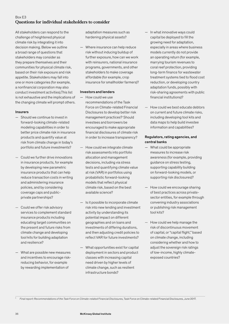
Box E3Questions for individual stakeholders to consider
1 Final report: Recommendations of the Task Force on Climate-related Financial Disclosures, Task Force on Climate-related Financial Disclosures, June 2017.
All stakeholders can respond to the challenge of heightened physical climate risk by integrating it into decision making. Below we outline a broad range of questions that stakeholders may consider as they prepare themselves and their communities for physical climate risk, based on their risk exposure and risk appetite. Stakeholders may fall into one or more categories (for example, a nonfinancial corporation may also conduct investment activities).This list is not exhaustive and the implications of the changing climate will prompt others.
Insurers — Should we continue to invest in
forward-looking climate-related modeling capabilities in order to better price climate risk in insurance products and quantify value at risk from climate change in today’s portfolio and future investments?
— Could we further drive innovations in insurance products, for example by developing new parametric insurance products that can help reduce transaction costs in writing and administering insurance policies, and by considering coverage caps and public-private partnerships?
— Could we offer risk advisory services to complement standard insurance products including educating target communities on the present and future risks from climate change and developing tool kits for building adaptation and resilience?
— What are possible new measures and incentives to encourage risk-reducing behavior, for example by rewarding implementation of
adaptation measures such as hardening physical assets?
— Where insurance can help reduce risk without inducing buildup of further exposure, how can we work with reinsurers, national insurance programs, governments, and other stakeholders to make coverage affordable (for example, crop insurance for smallholder farmers)?
Investors and lenders — How could we use
recommendations of the Task Force on Climate-related Financial Disclosures to develop better risk management practices?1 Should investees and borrowers be encouraged to make appropriate financial disclosures of climate risk in order to increase transparency?
— How could we integrate climate risk assessments into portfolio allocation and management decisions, including via stress tests and quantifying climate value at risk (VAR) in portfolios using probabilistic forward-looking models that reflect physical climate risk, based on the best available science?
— Is it possible to incorporate climate risk into new lending and investment activity by understanding its potential impact on different geographies and on loans and investments of differing durations, and then adjusting credit policies to reflect VAR for future investments?
— What opportunities exist for capital deployment in sectors and product classes with increasing capital need driven by higher levels of climate change, such as resilient infrastructure bonds?
— In what innovative ways could capital be deployed to fill the growing need for adaptation, especially in areas where business models currently do not provide an operating return (for example, marrying tourism revenues to coral reef protection, providing long-term finance for wastewater treatment systems tied to flood cost reduction, or developing country adaptation funds, possibly with risk-sharing agreements with public financial institutions)?
— How could we best educate debtors on current and future climate risks, including developing tool kits and data maps to help build investee information and capabilities?
Regulators, rating agencies, and central banks
— What could be appropriate measures to increase risk awareness (for example, providing guidance on stress testing, supporting capability building on forward-looking models, or supporting risk disclosures)?
— How could we encourage sharing of best practices across private-sector entities, for example through convening industry associations or publishing risk management tool kits?
— How could we help manage the risk of discontinuous movement of capital, or “capital flight,” based on climate change, including considering whether and how to adjust the sovereign risk ratings of low-income, highly climate-exposed countries?
36 McKinsey Global Institute
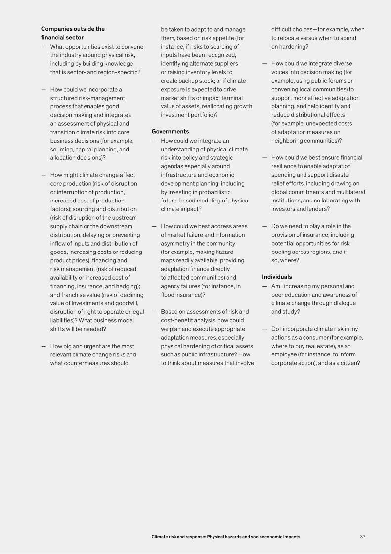
Companies outside the financial sector
— What opportunities exist to convene the industry around physical risk, including by building knowledge that is sector- and region-specific?
— How could we incorporate a structured risk-management process that enables good decision making and integrates an assessment of physical and transition climate risk into core business decisions (for example, sourcing, capital planning, and allocation decisions)?
— How might climate change affect core production (risk of disruption or interruption of production, increased cost of production factors); sourcing and distribution (risk of disruption of the upstream supply chain or the downstream distribution, delaying or preventing inflow of inputs and distribution of goods, increasing costs or reducing product prices); financing and risk management (risk of reduced availability or increased cost of financing, insurance, and hedging); and franchise value (risk of declining value of investments and goodwill, disruption of right to operate or legal liabilities)? What business model shifts will be needed?
— How big and urgent are the most relevant climate change risks and what countermeasures should
be taken to adapt to and manage them, based on risk appetite (for instance, if risks to sourcing of inputs have been recognized, identifying alternate suppliers or raising inventory levels to create backup stock; or if climate exposure is expected to drive market shifts or impact terminal value of assets, reallocating growth investment portfolio)?
Governments — How could we integrate an
understanding of physical climate risk into policy and strategic agendas especially around infrastructure and economic development planning, including by investing in probabilistic future-based modeling of physical climate impact?
— How could we best address areas of market failure and information asymmetry in the community (for example, making hazard maps readily available, providing adaptation finance directly to affected communities) and agency failures (for instance, in flood insurance)?
— Based on assessments of risk and cost-benefit analysis, how could we plan and execute appropriate adaptation measures, especially physical hardening of critical assets such as public infrastructure? How to think about measures that involve
difficult choices—for example, when to relocate versus when to spend on hardening?
— How could we integrate diverse voices into decision making (for example, using public forums or convening local communities) to support more effective adaptation planning, and help identify and reduce distributional effects (for example, unexpected costs of adaptation measures on neighboring communities)?
— How could we best ensure financial resilience to enable adaptation spending and support disaster relief efforts, including drawing on global commitments and multilateral institutions, and collaborating with investors and lenders?
— Do we need to play a role in the provision of insurance, including potential opportunities for risk pooling across regions, and if so, where?
Individuals — Am I increasing my personal and
peer education and awareness of climate change through dialogue and study?
— Do I incorporate climate risk in my actions as a consumer (for example, where to buy real estate), as an employee (for instance, to inform corporate action), and as a citizen?
37Climate risk and response: Physical hazards and socioeconomic impacts

Communities susceptible to flooding from storms and sea level rise in Manila. © George Steinmetz/National Geographic
1. Understanding physical climate risk
A changing climate is introducing new risks that are significant today and will grow. These risks can be grouped into three types: physical risk (risks arising from the physical effects of climate change); transition risk (risks arising from transition to a low-carbon economy); and liability risk (risks arising from those affected by climate change seeking compensation for losses).54 While some regions and sector could benefit, this report assesses the physical risk from a changing climate, including the potential effects on people, communities, natural and physical capital, and economic activity, and the implications for companies, governments, financial institutions, and individuals. We do not focus on transition risks or liability risks associated with climate change. While decarbonization and the risks and opportunities it creates is a critical topic, this report contributes by exploring the nature and costs of ongoing climate change in the absence of decarbonization.
Physical climate risks are probabilistic because of the probabilistic nature of the underlying climate hazards that create risk; for example, there is a certain likelihood associated with having floods of a given severity, or days above a certain temperature, in a year. By hazards, we mean climate-induced physical phenomena (acute or chronic) that have the potential to impact natural and socioeconomic systems. A changing climate means these likelihoods are shifting. We consider the “inherent” level of risk that results from these shifts —that is, the risk before consideration of adaptation and mitigation measures that could reduce the likelihood or magnitude of socioeconomic impacts—as well as the potential adaptation and mitigation response. We believe this approach is appropriate to help stakeholders understand the potential magnitude of the impacts from climate change and the commensurate response required. We look at two periods: between today and 2030, and from 2030 to 2050.
To develop meaningful local estimates of physical climate risk, we draw on climate models to understand how geospatially specific climate hazards could evolve under an RCP 8.5 scenario. We then create a taxonomy for physical risk by examining the impact of those hazards on five critical socioeconomic systems. They are: livability and workability, food systems, physical assets, infrastructure services, and natural capital. Together, these represent impacts on human beings, human-made physical assets, and the natural world. For each type of system, we assess impact by examining nine cases across sectors and geographies that were chosen based on their exposure to the extremes of climate change and their proximity today to key physical and biological thresholds. As such, they represent leading-edge examples of climate change. In a separate analysis, we use geospatial data to provide a perspective on physical climate risk across 105 countries over the next 30 years, using the same five-systems framework of direct impacts. Details of our modeling are described in the executive summary, Chapter 4, and the technical appendix.
54 Climate change: What are the risks to financial stability ? Bank of England, KnowledgeBank.
39Climate risk and response: Physical hazards and socioeconomic impacts
Our intent is not to provide point forecasts. Climate is the statistical summary of weather patterns over time and is therefore probabilistic in nature. Following standard practice, our findings are therefore framed as “statistically expected values”—the statistically expected average impact across a range of probabilities of different hazard manifestations. We also report the value of “tail risks”—that is, low-probability, high-impact events like a 1-in-100-year storm—on an annual basis. In some cases, we show the cumulative probability of a tail risk over a period. Consider for example a flooding event that has a 1 percent likelihood of occurrence every year (often described as a “100-year flood”). In the lifetime of home ownership, the cumulative likelihood that the home will experience at least one 100-year flood is 26 percent.55 Understanding such cumulative probabilities is important for stakeholders looking to design appropriate risk-management strategies.
A five-systems framework for measuring potential direct and indirect impacts of the changing climateWe measure the impact of climate change by the extent to which it could disrupt or destroy stocks of capital—human, physical, and natural—and the resultant socioeconomic impact of that disruption or destruction. As climate hazards manifest, they can affect these systems and thus create risk. For example, flooding in a particular location could damage a physical structure like a factory. To provide a framework for our analysis, we conducted an extensive review of direct impacts and classified them into five groups of system directly affected by physical climate hazards. The five are livability and workability, food systems, physical assets, infrastructure services, and natural capital. This five-systems impact framework is our best effort to capture the entire range of potential impacts from physical climate hazards. In the course of our work, we have not identified any other material impacts of climate change outside these five groups. We define each of the five as follows:
— Livability and workability. Livability refers to the ability of an area to sustain human life and activity; workability is the capacity to engage in outdoor work. Hazards like heat stress and flooding could affect the ability of human beings to work outdoors or put human lives at risk. Heat reduces labor capacity because workers must take breaks to avoid heatstroke and because the body naturally limits its efforts in order to prevent over-exertion. Increased temperatures could also shift disease vectors and thus affect human health.
— Food systems. Food systems include the production and distribution of agricultural products and the associated revenues and livelihoods. Food production could be disrupted as drought conditions, extreme temperatures, or floods affect land and crops. Conversely, some climatic shifts could also make some regions more suitable for agriculture. A changing climate change can both improve and degrade food system performance, while introducing more or less volatility. In some cases, crop yields may increase; in other cases, thresholds could be exceeded beyond which some crops fail entirely.
— Physical assets. Physical assets like buildings could be damaged or destroyed by extreme precipitation, tidal flooding, forest fires, and other hazards. Hazards could even materially impact an entire network of assets such as a city’s central business district.
— Infrastructure services. Infrastructure assets are a particular type of physical asset that could be destroyed in their functioning, leading to a decline in the services they provide or a rise in the cost of these services. For example, power systems could become less productive under very hot conditions. A range of hazards including heat, wind, and precipitation can disrupt infrastructure services. This in turn can have knock-on effects on other sectors.
55 Assuming that probabilities stay constant throughout the 30-year period.
40 McKinsey Global Institute

— Natural capital. Climate change is shifting ecosystems and destroying forms of natural capital such as glaciers, forests, and ocean ecosystems, which provide important services to humans. Natural capital is at risk from both acute hazards like wildfires and chronic hazards like rising temperatures. These impacts are hard to model but could be nonlinear and in some cases—such as glacier melting—irreversible. In some cases, human mismanagement may play a role, for example with forest fires and water scarcity, but the effect of this mismanagement is multiplied by climate change.
To assess the magnitude of direct physical climate risk in each case and for our geospatial analysis, we examine the severity of the hazard and its likelihood; the exposure of people, assets, or economic activity to the hazard; and the extent to which systems are vulnerable to the hazard, for example, how vulnerable buildings are to damage from different depths of flood. Direct impacts could have knock-on effects. For example, flood damage to a factory could interrupt production and affect downstream players in a supply chain.
How our methodology addresses possible sources of uncertaintyOne of the main challenges in understanding the physical risk arising from climate change is the range of uncertainties involved. Yet a key insight of this research has been that, despite the many uncertainties associated with estimations of impact from a changing climate, it is possible for the science and socioeconomic analyses and methodologies presented here to provide actionable insights. In this chapter, we outline some of these uncertainties and our approach to addressing them. It is important for decision makers to understand these uncertainties and incorporate that understanding into a risk-management approach that aligns with their risk appetite.
Here, we highlight the possible sources of uncertainty and our methodological approach to addressing these in this report. The discussion below relates both to the results from our case studies and from our geospatial analysis. Risks arise as a result of an involved causal chain: Emissions influence both global climate as well as regional climate variations, which in turn influence the frequency and severity of specific climate hazards (such as droughts and sea-level rise), which then influence the frequency and severity of physical damage (such as crop shortage and infrastructure damages), which finally influence broader economic, social and financial harm. Our analysis, like any such effort, relies on assumptions made along the causal chain: about emission paths and adaptation schemes; global and regional climate models; physical damage functions; and knock-on effects. The further one goes along the chain, the greater the intrinsic model uncertainty.
The key uncertainties include: emissions pathways and the pace of warming; climate model accuracy and natural variability; the magnitude of direct and indirect socioeconomic impacts, given a certain hazard; and the socioeconomic response.
Emissions pathways and pace of warmingClimate impact research has inherent uncertainties and as a result makes extensive use of scenarios. One particular input around which scenarios are frequently constructed is atmospheric greenhouse gas levels. Projections of future climate must be based upon an assumed trajectory for future atmospheric greenhouse gas concentrations. Because future human emissions of greenhouse gases are inherently unpredictable, the climate community has developed a set of four standardized scenarios for future atmospheric greenhouse gas concentrations, known as Representative Concentration Pathways (RCPs). 56 They outline different atmospheric greenhouse gas concentration trajectories between 2005 and 2100 that roughly range from lower (RCP2.6) to higher (RCP 8.5) CO2 concentrations. During their inception, RCPs were designed to collectively sample the range of then-probable future emission pathways. Each RCP was created by an independent modeling team and there is
56 Detlef P. van Vuuren et al., “The Representative Concentration Pathways: An overview,” Climatic Change, November 2011, Volume 109, Issue 1–2.
41Climate risk and response: Physical hazards and socioeconomic impacts

no consistent design of the socioeconomic parameter assumptions used in the derivation of the RCPs.
Uncertainty in future greenhouse gas emissions is a key contributor to long-term (for example, end-of-century) uncertainty in future temperatures but is less important on the shorter time horizons (out to 2050) considered in this report. As we discuss in detail in Chapter 2, warming during the next decade is determined largely by past emissions and by physical inertia in the climate system. Beyond the next decade, warming is primarily a function of cumulative emissions of carbon dioxide. Because decarbonization takes time, even a scenario of targeted decarbonization action will result in significant cumulative emissions over the next three decades. Climate simulations driven by the four RCP scenarios show a small divergence in warming over the next two decades, and a moderate divergence by 2050 (see also Exhibit 1, which shows projected warming for RCP 8.5 and RCP 4.5; the two RCPs that are most commonly used in climate models, to provide a sense of the spread in scenarios).57
We rely on RCP 8.5 for the analyses in this report. RCP 8.5 was created to model a case of no further climate action and relatively higher rates of baseline greenhouse gas emissions. We have chosen to focus on RCP 8.5, because the higher-emission scenario it portrays enables us to assess physical risk in the absence of further decarbonization.
While RCP 8.5 has been criticized for assuming unrealistically high use of coal and thus projecting too-high emissions in the second half of the century, we only consider a timeframe out to 2050, and we adopted RCP 8.5 as a best available description for an ‘inherent risk’ scenario over the next two to three decades.58
This assessment was also made for the following reasons.
— Since the starting point of the RCPs in 2005, RCP 8.5 has most closely tracked actual greenhouse gas emissions (and going forward, RCP 8.5 is broadly consistent with a continuation of the emissions trend of the last decade).59 As a result, it best matches current CO2 concentrations, whereas the other RCPs assume lower CO2 concentrations than observed.
— Changes in the relative cost of renewable and fossil energy sources are forecast to lead to a moderate downward divergence from the historic trendline of energy-related CO2 emissions over the coming decades, even in absence of further decarbonization policies.60 In contrast, emissions from biotic feedbacks, such as permafrost thaw or increasing wildfires, are expected to increase. These feedbacks are not considered in the current generation of CMIP5 models and need to be accounted for exogenously. According to a recent review of the literature on biotic feedbacks, in the near term these feedbacks are estimated to reduce the 1.5 degree Celsius carbon budget by 100 GtCO2, and 2 degree Celsius carbon budget by 150 GtCO2.61
57 Ibid.58 Justin Ritchie and Hadi Dowlatabadi, “The 1000 GtC coal question: Are cases of vastly expanded future coal combustion
still plausible?” Energy Economics, June 2017, Volume 65; Justin Ritchie and Hadi Dowlatabadi, “Why do climate change scenarios return to coal?” Energy, December 2017, Volume 140, Part 1; Keywan Riahi et al., “The Shared Socioeconomic Pathways and their energy, land use, and greenhouse gas emissions implications: An overview,” Global Environmental Change, January 2017, Volume 42; Keywan Riahi, Arnulf Grübler, and Nebojsa Nakicenovic, “Scenarios of long-term socio-economic and environmental development under climate stabilization,” Technological Forecasting and Social Change, September 2007, Volume 74, Issue 7; Detlef P. van Vuuren et al., “The Representative Concentration Pathways: An overview,” Climatic Change, November 2011, Volume 109, Issue 1–2.
59 Hayhoe, K., J. Edmonds, R.E. Kopp, A.N. LeGrande, B.M. Sanderson, M.F. Wehner, and D.J. Wuebbles, 2017: Climate models, scenarios, and projections. In: Climate Science Special Report: Fourth National Climate Assessment, Volume I [Wuebbles, D.J., D.W. Fahey, K.A. Hibbard, D.J. Dokken, B.C. Stewart, and T.K. Maycock (eds.)]. U.S. Global Change Research Program, Washington, DC, USA, pp. 133-160, doi: 10.7930/J0WH2N54.
60 IEA World Energy Outlook 2019.61 Jason A Lowe and Daniel Bernie, “The impact of Earth system feedbacks on carbon budgets and climate response,”
Philosophical Transactions of the Royal Society A, May 2018, Volume 376, Number 2119.
42 McKinsey Global Institute

— Early results from the next generation of climate models, CMIP6, suggest that the climate system may be more sensitive to CO2 than the current generation of models (CMIP5) used here, suggesting that the CMIP5 models may tend to underestimate future warming.62
Based upon these considerations we chose to employ RCP 8.5 as a base case for considering 2030 to 2050. Were this study investigating the risk outlook for 2100, we would consider multiple emissions pathways, but for the next three decades, we consider RCP 8.5 to be the best guide for understanding inherent risk.
Restricting warming to below two degrees, the goal of the 2015 Paris agreement, would mean reaching net-zero emissions in the next 40 to 50 years. If this were achieved, the impact estimates presented in this report would likely not manifest to their full extent. Alternately, a decarbonization approach somewhere between business-as-usual and a two-degree-compliant pathway would mean that temperatures in 2050 would be below the roughly 2 degrees Celsius increase reflected in the RCP 8.5 scenario, but that such temperature increases would be reached at some point post-2050. This means that the impact assessments presented in this report would manifest but only after 2050; it would push the 2050 impacts further back into the second half of the century but would not prevent them.
Another way to frame this would be that if we were to limit warming to 2 degrees Celsius, our 2050 impact estimates would be the most severe impacts we would be expected to see (but at some point after 2050), and if we were to limit warming to 1.5 degrees Celsius, correspondingly our 2030 impact estimates would be the most severe impacts we would be expected to see (but at some point after 2030). For example, RCP 8.5 predicts global average warming of 2.3 degrees Celsius by 2050, compared with 1.8 for RCP 4.5. Under RCP 4.5, 2.3 degrees Celsius warming would be reached in the year 2080.63
Climate model accuracyThis refers to modeling uncertainty associated with climate models that translate greenhouse gas emissions into temperature increases and effects on other hazards, both globally and in specific regions. While uncertainty is inherent in any model, scientists have tested the ensemble of climate models used in this report against both observations and paleoclimate records, and as a result have confidence in their probabilistic predictions of how climate hazards will evolve over the next decades, given a particular emissions pathway.64 To reduce model error, this report uses the mean or median projection of an ensemble of models, depending on the requirements of the specific analysis.65 This approach has been found to generate a more robust projection than any individual model.66 It is important to note that, when looking across a full range of climate science models, the uncertainty in global temperatures tends to skew primarily toward worse rather than better outcomes (Exhibit 1).
62 Stephen Belcher, Olivier Boucher, and Rowan Sutton, Why results from the next generation of climate models matter, Carbon Brief, March 2019.
63 Intergovernmental Panel on Climate Change (IPCC), 2014: Annex II: Climate System Scenario Tables, 2013. 64 Gregory Flato et al., “Evaluation of climate models,” in Climate Change 2013: The Physical Science Basis. Contribution of
Working Group I to the Fifth Assessment Report of the Intergovernmental Panel on Climate Change, Thomas F. Stocker et al., eds., New York, NY: Cambridge University Press, 2014; Sandy P. Harrison, Patrick J. Bartlein, and I. Colin Prentice, “What have we learnt from paleoclimate simulations ?” Journal of Quaternary Science, May 2016, Volume 31, Number 4; Zeke Hausfather, “Analysis: How well have climate models projected global warming ?” Carbon Brief, 2017.
65 For most of the analysis used in the report, we rely on analysis from the Woods Hole Research Center (WHRC) on an ensemble of climate models, as described here. In some instances (for example, modeling changes in water supply), we have relied on publicly available data sets showcasing shifts in climate hazards. This has been noted where relevant.
66 See the technical appendix for further details.
43Climate risk and response: Physical hazards and socioeconomic impacts
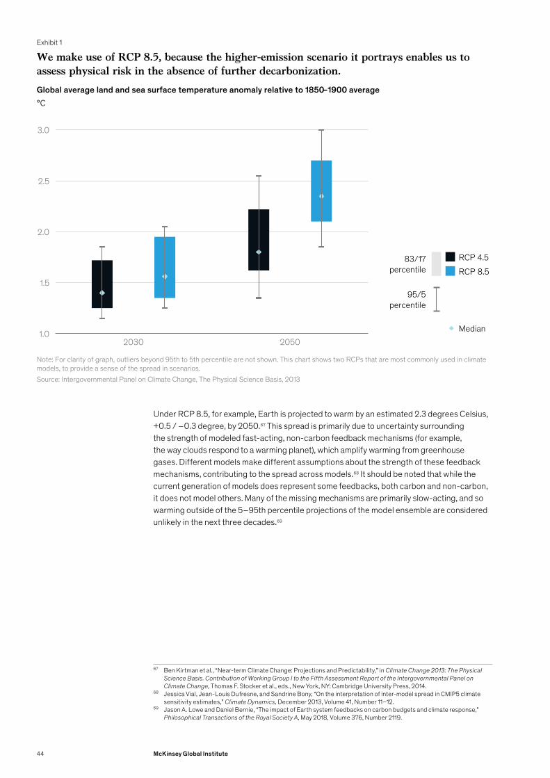
Under RCP 8.5, for example, Earth is projected to warm by an estimated 2.3 degrees Celsius, +0.5 / –0.3 degree, by 2050.67 This spread is primarily due to uncertainty surrounding the strength of modeled fast-acting, non-carbon feedback mechanisms (for example, the way clouds respond to a warming planet), which amplify warming from greenhouse gases. Different models make different assumptions about the strength of these feedback mechanisms, contributing to the spread across models.68 It should be noted that while the current generation of models does represent some feedbacks, both carbon and non-carbon, it does not model others. Many of the missing mechanisms are primarily slow-acting, and so warming outside of the 5–95th percentile projections of the model ensemble are considered unlikely in the next three decades.69
67 Ben Kirtman et al., “Near-term Climate Change: Projections and Predictability,” in Climate Change 2013: The Physical Science Basis. Contribution of Working Group I to the Fifth Assessment Report of the Intergovernmental Panel on Climate Change, Thomas F. Stocker et al., eds., New York, NY: Cambridge University Press, 2014.
68 Jessica Vial, Jean-Louis Dufresne, and Sandrine Bony, “On the interpretation of inter-model spread in CMIP5 climate sensitivity estimates,” Climate Dynamics, December 2013, Volume 41, Number 11–12.
69 Jason A. Lowe and Daniel Bernie, “The impact of Earth system feedbacks on carbon budgets and climate response,” Philosophical Transactions of the Royal Society A, May 2018, Volume 376, Number 2119.
Exhibit 1
We make use of RCP 8.5, because the higher-emission scenario it portrays enables us to assess physical risk in the absence of further decarbonization.
Source: Intergovernmental Panel on Climate Change, The Physical Science Basis, 2013
Global average land and sea surface temperature anomaly relative to 1850–1900 average°C
1.0
1.5
2.0
2.5
3.0
2030 2050
RCP 4.5RCP 8.5
83/17 percentile
95/5 percentile
Median
NOTE!
Many exhibits repeat between ES, Report,
Apx, and Cases.
Be sure to copy repeats to all places!
Note: For clarity of graph, outliers beyond 95th to 5th percentile are not shown. This chart shows two RCPs that are most commonly used in climate models, to provide a sense of the spread in scenarios.
44 McKinsey Global Institute
Modeling climate changes at a regional level introduces additional sources of uncertainty. Because global climate models are generally spatially coarse, on the order of 100 by 100 kilometers, they are unable to resolve, or simulate, small geographical, atmospheric, or biological features that exert significant influence over local climates. The global climate system can also distribute additional heat in multiple different ways, and so the same emissions scenario can result in different regional warming outcomes.70 Some of this uncertainty can be reduced through technical methods (for example, the use of historical regional data to calibrate global climate models), and some cannot.71 To make “skillful” regional predictions requires careful choices of the specific modeling tool, climatic variable of interest, region, and time period.72 The analyses in this study have been designed in such a way as to minimize uncertainty from regional natural variability (through region, time period, and variable choice), as well as to minimize uncertainty from model error (through technical methods).73 For more details, see the technical appendix.
Natural variabilityNatural variability is another consideration influencing how hazards could evolve. It refers to climatic changes that occur independently of changes in the amount of energy trapped in the Earth system. Natural variability arises primarily from multiyear patterns in ocean circulation that can temporarily warm or cool the surface of the planet. These changes are included in climate models, but because of their stochastic, or random, nature, their timing cannot be accurately projected.74 One example is the El Niño / La Niña oscillation. Another is the so-called global warming hiatus between 1998 and 2012, during which the global average temperature did not seem to increase as much as climate models projected, as warming of the planet’s surface was masked by changes in ocean heat uptake.75 The presence of natural variability introduces uncertainty into our projections because it can temporarily accelerate or delay the manifestation of longer-term statistical climate shifts.76 This uncertainty will be particularly important over the next decade, during which overall climatic shifts relative to today may be smaller in magnitude than a potential acceleration or delay in warming due to natural variability.77
Direct and indirect socioeconomic impactsTo measure direct impact as hazards manifest, we have relied on publicly available vulnerability assessments or “damage functions” for this but note that they may not accurately represent the vulnerability of a specific asset or location. Another factor that could create uncertainty is the magnitude of exposure to climate hazards. If more people or assets are located in regions that are exposed to climate hazards, impacts could be higher. For this report, we assume that exposure is constant for instances where we do not expect significant shifts in exposure—for example, when we consider breadbasket failures, we do not assume significant shifts in where crops are grown today. In other instances, we do consider changes in exposure, such as sectoral shifts out of agriculture and manufacturing in the case of the
70 Clara Deser et al., “Communication of the role of natural variability in future North American climate,” Nature Climate Change, October 26, 2012.
71 Ed Hawkins and Rowan Sutton, “The potential to narrow uncertainty in regional climate predictions,” Bulletin of the American Meteorological Society, August 2009, Volume 90, Number 8.
72 A “skillful” prediction in the climate-science context refers to the ability of a climate model to produce accurate or robust projections of change in a given variable (for example, daily maximum temperature) over a given area and time scale.
73 Ed Hawkins and Rowan Sutton, “The potential to narrow uncertainty in regional climate predictions,” Bulletin of the American Meteorological Society, August 2009, Volume 90, Number 8; Nurul Nadrah Aqilah Tukimat, “Assessing the implementation of bias correction in the climate prediction,” IOP Conference Series: Materials Science and Engineering, April 2018; Gerhard Krinner and Mark G. Flanner, “Striking stationarity of large-scale climate model bias patterns under strong climate change,” Proceedings of the National Academy of Sciences, September 2018, Volume 115, Number 38.
74 Kyle L. Swanson, George Sugihara, and Anastasios A. Tsonis, “Long-term natural variability and 20th century climate change,” Proceedings of the National Academy of Sciences, September 2009, Volume 106, Number 38.
75 While the planet continued to warm during this period, the warming was masked by changes in ocean heat uptake, which can produce temporary average global surface temperature trends of +/– 0.25 degree on time scales of up to a decade. Given that global surface temperature warming is currently occurring at approximately 0.2 degree per decade, the warming trend was obfuscated during the 1998–2012 period. Iselin Medhaug et al., “Reconciling controversies about the ‘global warming hiatus,’” Nature, May 2017, Volume 545; Zeke Hausfather et al., “Assessing recent warming using instrumentally homogeneous sea surface temperature records,” Science Advances, January 2017, Volume 3, Number 1.
76 Ed Hawkins and Rowan Sutton, “The potential to narrow uncertainty in regional climate predictions,” Bulletin of the American Meteorological Society, August 2009, Volume 90, Number 8.
77 Ibid.
45Climate risk and response: Physical hazards and socioeconomic impacts
impact of heat on India. We also consider increased infrastructure buildup when we look at the impact of flooding on cities in developing countries.
Finally, there is uncertainty related to the indirect, or knock-on, impacts of a changing climate. Given the complexity of socioeconomic systems, we know that our case results do not capture the full impact of climate change. Socioeconomic systems are dynamic, with many interacting and interdependent elements. As is typical for such systems, changes in one element can have nonlinear repercussions on other elements and lead to unexpected phenomena. Assessing possible social or political knock-on effects from phenomena like lethal heat waves, for example, is difficult, and we have almost certainly not identified the full range of knock-on effects (see Box 1, “Three channels through which climate risk could trigger disruption in extreme cases”). Even in instances where we have identified knock-on effects, sizing the magnitude of potential impact in a given case—for example, the degree to which real estate valuations in Florida could change and when—is difficult. In many cases, we have relied either on past trends and empirical estimates of knock-on effects or discussed them in a qualitative manner alone.
Socioeconomic responseHow much risk manifests also depends on the robustness of the response to the risk that is forecast. Adaptation measures such as hardening physical infrastructure, relocating people and assets, and ensuring backup capacity, among others, can help manage the impact of climate hazards and reduce risk. We therefore follow an approach that first assesses the inherent risk and then considers a potential adaptation response. We have not conducted a detailed bottom-up cost-benefit analysis of adaptation measures but have built on existing literature and expert interviews to understand the most important measures and their indicative cost, effectiveness, and implementation challenges in each of our cases, and to estimate the expected global adaptation spending required. While we note the critical importance of decarbonization in an appropriate climate risk management approach, a detailed road map for decarbonization is beyond the scope of this report.
We conclude that despite many uncertainties that need to be reflected in decision making, climate science and the socioeconomic analyses and methodologies presented here can provide actionable insights for decision makers. Uncertainties tend to be skewed toward larger rather than smaller impact. How decision makers incorporate these uncertainties into their management choices will depend on their risk appetite and overall risk management approach. Some may want to work with the outcome considered most likely (which is what we generally considered with our analysis of “statistically expected outcomes”), while others may want to consider a worse- or even worst-case scenario. Given the complexities we have outlined above, we recognize that more research is needed in this critical field.
46 McKinsey Global Institute
Box 1Three channels through which physical climate risk could trigger disruption in extreme cases
1 A “Minsky moment”—named for the American economist Hyman Minsky—is the onset of a market collapse brought on by the reckless speculative activity that defines an unsustainable bullish period. For a discussion of how climate risks could create a Minsky moment that disrupts financial markets, see Mark Carney, A Transition in Thinking and Action, speech at the International Climate Risk Conference for Supervisors, De Nederlandsche Bank, Amsterdam, April 6, 2018.
2 Sylvain Ponserre and Justin Ginnetti, Disaster displacement: A global review, 2008–2018, Internal Displacement Monitoring Centre, May 2019.
3 Kanta Kumari Rigaud et al., Groundswell: Preparing for internal climate migration, World Bank, March 2018.4 2014 quadrennial defense review, US Department of Defense, 2014.
As physical climate risk spreads beyond local economies, it could trigger broader economic, financial, social, and political disruption. While the likelihood and potential magnitude of such disruption is impossible to predict, it could occur through several channels, including the following three.
First, physical risks—and the anticipation thereof—which may prompt an abrupt policy response. Sudden regulatory responses to rising climate hazards, for example following a series of natural disasters or a marked change in political priorities, could destabilize markets and companies. Such an abrupt transition would leave companies across the world with assets that could become too expensive or even impossible to operate. This could in turn lead to a range of knock-on effects for the owners of the asset, their ability to finance other assets, and creditworthiness.
Second, sudden asset repricing and capital reallocation. Financial markets could experience a devaluation due to an abrupt repricing of assets or a loss of access to long-term capital. Such a climate “Minsky moment” might occur if a significant number of market participants were to come to believe they have not adequately factored in physical climate risks which could lead to a sudden depreciation of, for example, real estate prices.1 Knock-on financial effects could then result from such a depreciation of collateral depending on the degree of leverage, complexity (securitization and pooling), and transparency around the financing of those assets. As an example, significant storm surge losses from hurricanes hitting coastal real estate could lead to a substantial rise in insurance premiums, followed by an abrupt devaluation of that real estate market, which in turn might lead investors to reappraise their investments in other coastal real estate markets. A recognition by capital markets of projected hazards and possible impacts over the coming decades could also lead to changes in the cost or availability of long-term capital for certain sectors or regions and to changes in credit ratings, disclosure, and regulations which could have the potential of creating a period of heightened uncertainty and illiquidity until ratings, information, and regulation meet the new market expectations. Unlike other financial sector booms and busts, the downside risk in climate change-driven depreciation would likely not be cyclical—it would reflect higher long-lasting, structural risks in particular geographies or sectors—hence requiring structural responses. A swing from not considering climate risk to extreme caution in climate-sensitive assets is a real concern.
Third, disruptive relocation of population and assets. Severe climate change effects could trigger migration, social and political unrest, and potentially even conflict in affected regions, which in turn may have global repercussions. Between 2008 and 2018, natural disasters displaced as many as 265 million people, according to the Internal Displacement Monitoring Centre.2 The World Bank projects that by 2050, in Latin America, South Asia, and sub-Saharan Africa, climate change may cause about 140 million people to migrate within their countries, away from areas with lower water availability and crop productivity or rising sea level and storm surges.3 While climate change is often not the sole factor in migration decisions, it may amplify existing motivations such as poverty, war, and strife. As early as 2014, the US Department of Defense identified climate change as a “threat multiplier” and “accelerant of instability.”4
47Climate risk and response: Physical hazards and socioeconomic impacts
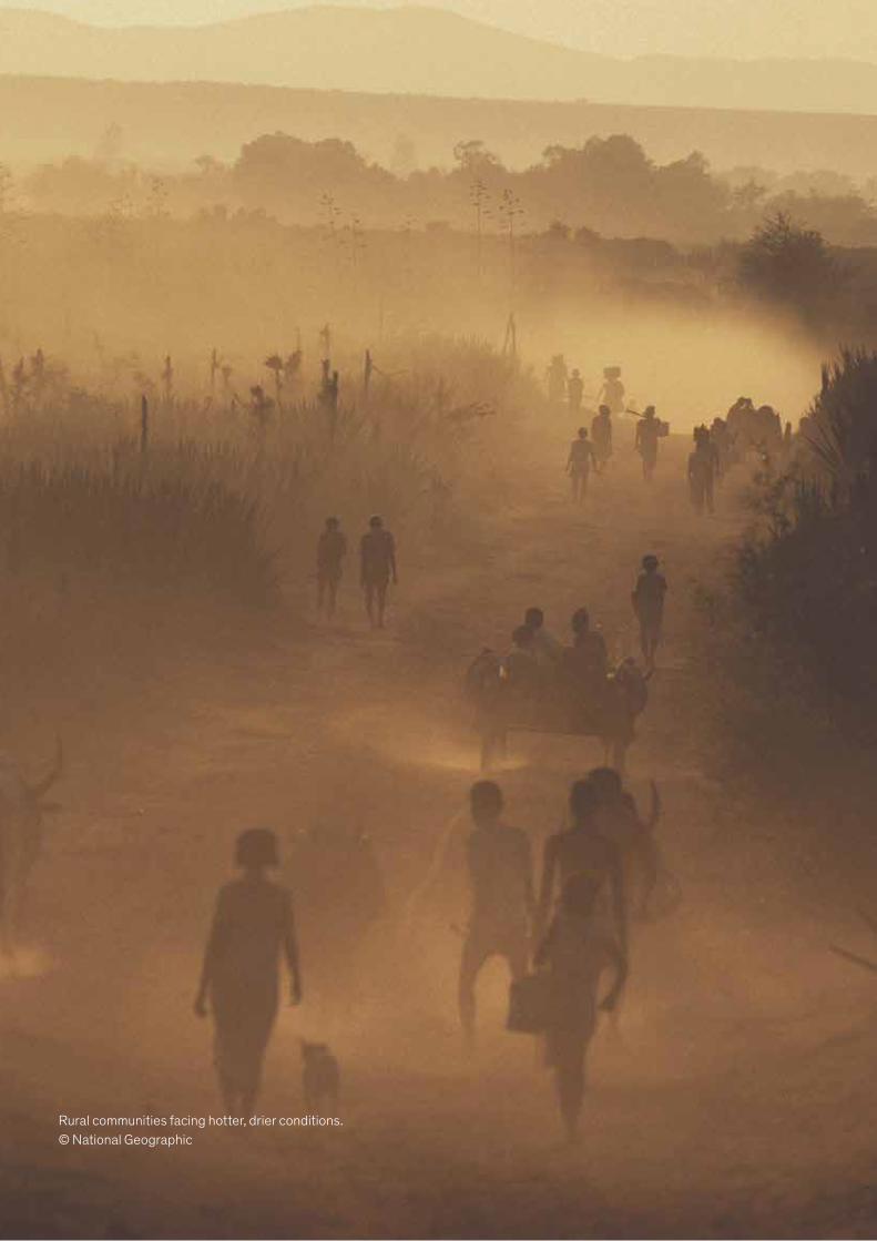
Rural communities facing hotter, drier conditions. © National Geographic

2. A changing climate and resulting physical riskA changing climate requires us to assess the impact of physical climate risk over time horizons relevant for decision makers today. Energy trapped by increasing atmospheric greenhouse gases leads to rising temperatures, which in turn intensifies chronic climate hazards and increases the frequency and or severity of acute events. These developments have an impact on socioeconomic systems around the world. Looking ahead, climate science tells us that additional warming is locked in for the next decade, regardless of mitigation measures that may be adopted. Beyond the next decade, further warming will occur as a function of cumulative emissions of long-lived greenhouse gases, like carbon dioxide. Climate science tells us that further warming and risk increase can only be stopped by achieving zero net greenhouse gas emissions. As the Earth continues to warm, climate science finds that physical climate hazards will intensify.
Earth’s climate is warming and climate hazards are intensifying During the past 2.6 million years or so of Earth’s 4.5-billion-year history, the planet oscillated between long cooling, or glacial, periods during which large ice sheets covered as much as one-third of the planet’s surface, and short warming, or interglacial, periods when the climate was more temperate for, typically, 10,000 to 30,000 years. For approximately the past 12,000 years, Earth has been in an interglacial period, characterized by a relatively stable, temperate climate. During this time, human civilization developed. Roughly 10,000 years ago, relatively soon after the climate stabilized, humans made the shift from hunter-gatherers to farmers (Exhibit 2).
Modern society was built during this time of stable climate, which shaped the world in three fundamental ways. First, it produced a habitable planet, allowing humans to spread across the world. Second, it shaped the design of physiological, human-made and ecological systems that are optimized for historical local climate parameters. For example, the choice of which crops to grow where and the engineering design standards used for infrastructure are both based on temperature and precipitation levels from this stable past. Third, the stable climate created a predictable physical environment, which contributed to the emergence of the modern economy. Much of the economic and financial activity, particularly for the long-term—including buying, selling, investing, borrowing, and lending—requires a degree of confidence that tomorrow will be similar to today.
49Climate risk and response: Physical hazards and socioeconomic impacts

This is now changing. The average combined global land-and-sea-surface temperature has increased by 1.1 +/– 0.05 degrees Celsius since 1880 (Exhibit 3).78 This has been confirmed by both satellite measurements and the analysis of hundreds of thousands of independent weather station observations from across the globe. The rapid decline in the planet’s surface ice cover provides further evidence. Earth is warming at a rate of about 0.2 degree Celsius per decade and losing Arctic sea ice at roughly 3,000 cubic kilometers per decade.79 This rate of warming is at least an order of magnitude faster than any currently identified in the past 65 million years of paleoclimate records and could be unprecedented as far back as 250 million years.80
78 NASA GISTEMP (2019) and, Nathan J. L. Lenssen et al., “Improvements in the GISTEMP uncertainty model,” Journal of Geophysical Resources: Atmospheres, June 2019, Volume 124, Number 12.
79 National Aeronautics and Space Administration (NASA) Goddard Institute for Space Studies (GISS), 2019; University of Washington Polar Science Center PIOMAS, 2019.
80 Noah S. Diffenbaugh and Christopher B. Field, “Changes in ecologically critical terrestrial climate conditions,” Science, August 2013, Volume 341, Number 6145; Seth D. Burgess, Samuel Bowring, and Shu-zhong Shen, “High-precision timeline for Earth’s most severe extinction,” Proceedings of the National Academy of Sciences, March 2014, Volume 111, Number 9.
Exhibit 2
350
300
150
200
250
400
450
AverageCO2 con-centrationin inter-glacialperiods
-4
-8
0
2
-6
-2
4
50350 300 250 200 150 100 0
0°C
Human civilization developed during a period of relatively stable climate.
Source: Bereiter et al., 2015; Feynman and Ruzmaikin, 2018; Uemura et al., 2012; McKinsey Global Institute analysis
Atmos-phericCO2
Parts per million by volume
Temper-atureanomaly relative to pre-indus-trial Holo-ceneclimate°C
YearsThousand
Today
150
25 20 15 0510
First agricultural societies established
Most recent glacial period
First Homo sapiens move out of Africa
First agricultural societies established
Most recent glacial period
50 McKinsey Global Institute
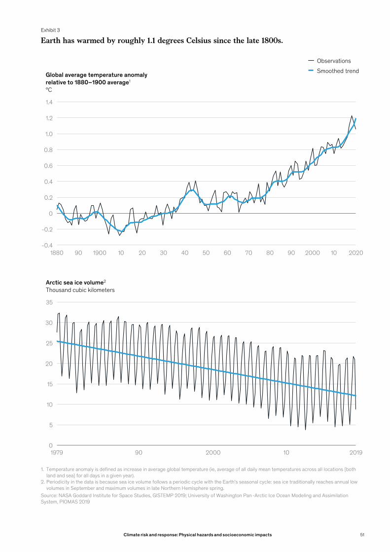
Exhibit 3
Earth has warmed by roughly 1.1 degrees Celsius since the late 1800s.
Source: NASA Goddard Institute for Space Studies, GISTEMP 2019; University of Washington Pan -Arctic Ice Ocean Modeling and Assimilation System, PIOMAS 2019
1. Temperature anomaly is defined as increase in average global temperature (ie, average of all daily mean temperatures across all locations [both land and sea] for all days in a given year).
2. Periodicity in the data is because sea ice volume follows a periodic cycle with the Earth’s seasonal cycle: sea ice traditionally reaches annual low volumes in September and maximum volumes in late Northern Hemisphere spring.
1.0
-0.4
0.4
0.2
-0.2
0
0.6
0.8
1.2
1.4
Global average temperature anomalyrelative to 1880–1900 average1
ºC
ObservationsSmoothed trend
0
20
5
10
30
15
35
25
Arctic sea ice volume2
Thousand cubic kilometers
1880 90 1900 10 20 30 40 50 60 70 80 90 2000 10 2020
1979 90 2000 10 2019
51Climate risk and response: Physical hazards and socioeconomic impacts
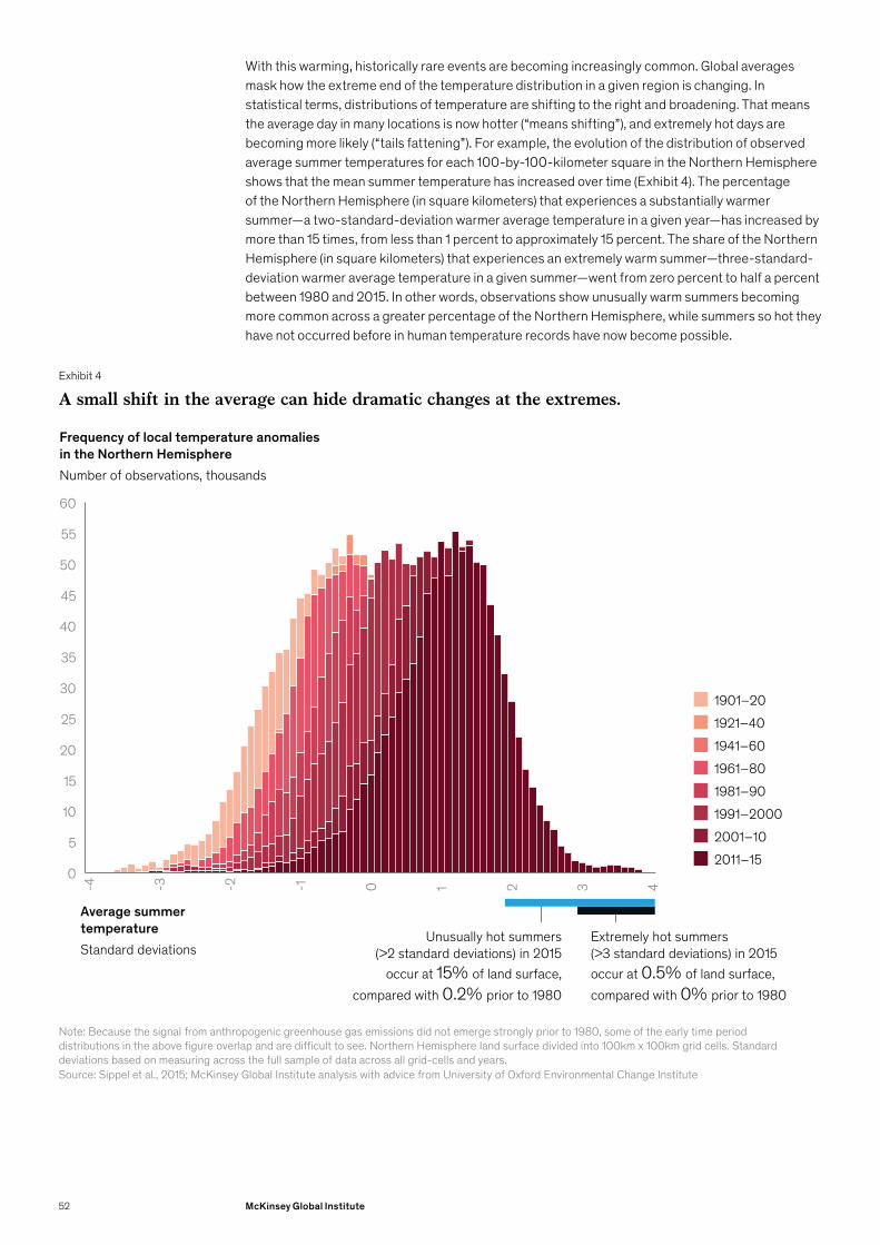
With this warming, historically rare events are becoming increasingly common. Global averages mask how the extreme end of the temperature distribution in a given region is changing. In statistical terms, distributions of temperature are shifting to the right and broadening. That means the average day in many locations is now hotter (“means shifting”), and extremely hot days are becoming more likely (“tails fattening”). For example, the evolution of the distribution of observed average summer temperatures for each 100-by-100-kilometer square in the Northern Hemisphere shows that the mean summer temperature has increased over time (Exhibit 4). The percentage of the Northern Hemisphere (in square kilometers) that experiences a substantially warmer summer—a two-standard-deviation warmer average temperature in a given year—has increased by more than 15 times, from less than 1 percent to approximately 15 percent. The share of the Northern Hemisphere (in square kilometers) that experiences an extremely warm summer—three-standard-deviation warmer average temperature in a given summer—went from zero percent to half a percent between 1980 and 2015. In other words, observations show unusually warm summers becoming more common across a greater percentage of the Northern Hemisphere, while summers so hot they have not occurred before in human temperature records have now become possible.
Exhibit 4
A small shift in the average can hide dramatic changes at the extremes.
0
5
10
20
15
30
25
35
40
45
50
55
60
Average summer temperatureStandard deviations
2-4 0-1
Frequency of local temperature anomalies in the Northern HemisphereNumber of observations, thousands
-3 -2 1 3 4
Source: Sippel et al., 2015; McKinsey Global Institute analysis with advice from University of Oxford Environmental Change Institute
Note: Because the signal from anthropogenic greenhouse gas emissions did not emerge strongly prior to 1980, some of the early time period distributions in the above figure overlap and are difficult to see. Northern Hemisphere land surface divided into 100km x 100km grid cells. Standard deviations based on measuring across the full sample of data across all grid-cells and years.
1901–20
1981–90
1921–401941–601961–80
1991–20002001–102011–15
Unusually hot summers (>2 standard deviations) in 2015
occur at 15% of land surface, compared with 0.2% prior to 1980
Extremely hot summers (>3 standard deviations) in 2015 occur at 0.5% of land surface, compared with 0% prior to 1980
52 McKinsey Global Institute

Averages also conceal wide spatial disparities. Over the same period that the Earth warmed by 1.1 degrees Celsius, in southern parts of Africa and the Arctic, average temperatures have risen by 0.2 to 0.5 degree and by 4 to 4.3 degrees, respectively.81 In general, the land surface has warmed faster than the 1.1-degree global average, and the oceans, which have a higher heat capacity, have warmed less. As average temperatures rise, acute hazards such as heat waves, extreme precipitation, and forest fires grow in frequency and or severity, and chronic hazards such as drought and rising sea levels intensify.82 Hotter summers and warmer winters change frequency and volume of precipitation, increasing risks of severe drought and extreme flooding. Rising temperatures also cause sea-level rise via the thermal expansion of water and melting of land ice, as well as increasing tropical storm severity and the risk of forest fires.83 Some of these hazard-specific trends are already identifiable. For example: since 1950, increases in the frequency and severity of heat waves have already been positively identified in Asia, Australia, and Europe. Increases in frequency and severity of extreme precipitation events have been identified in North America. Increases in drought frequency and severity have been identified in the Mediterranean and West Africa, while decreases have been identified in central North America.84
A changing climate affects socioeconomic systemsClimate change is already having an impact on human, physical, and natural systems. Across the world, we find examples of these impacts across each system in our five-systems framework (Exhibit 5). Researchers have found that in each case climate change intensified the natural hazard or increased its likelihood. For example:
— Hurricane Harvey, which made landfall in Texas on August 25, 2017, caused about $125 billion in damage and shut down economic activity for weeks, including about 20 percent of US crude oil refining capacity and a similar share of production in the Gulf of Mexico. Research suggests that the hurricane precipitation was about 8 to 19 percent more intense because of climate change.85
— Recent floods in Asia provide another example of economic damage. The 2017 Hunan province floods affected 7.8 million people and resulted in $3.55 billion of direct economic loss, including severe infrastructure damage. Researchers estimate that climate change made the floods twice as likely.86
— The July 2019 heat wave in Europe exceeded 37.5 degrees Celsius across the United Kingdom, the Netherlands, France, Germany, Italy, Spain, and Belgium, taking a toll on the region’s physical infrastructure, such as rail, roads, and power. This led to noticeable delays in transportation and to power outages. Economic activity slowed as small businesses and restaurants without air-conditioning closed.87 Climate change made this heat wave approximately 10 times more likely in France, according to academic research.88
81 Goddard Institute for Space Studies (GISS), GISTEMP Reanalysis dataset (2019).82 By hazards, we mean climate-induced physical events that have the potential to impact natural and socioeconomic
systems.83 Predictions of how Earth is likely to respond to further greenhouse gas emissions are drawn primarily from climate
models: computer simulations based on our understanding of physical laws and observations, laboratory experiments, and investigations into the past. These models simulate the atmosphere, ocean, land surface, and in some cases biosphere at resolutions down to tens of kilometers. They have proved successful at replicating past climates and at predicting more recent global and regional changes. Using those tools, it is possible to identify how climate hazards are likely to change by 2030 and 2050 around the world and to translate that to potential socioeconomic impact. See the technical appendix for more details.
84 D. L. Hartmann et al., “Observations: Atmosphere and Surface,” in Climate Change 2013: The Physical Science Basis. Contribution of Working Group I to the Fifth Assessment Report of the Intergovernmental Panel on Climate Change, Thomas F. Stocker et al., eds., New York, NY: Cambridge University Press, 2014.
85 Geert Jan van Oldenborgh et al., “Attribution of extreme rainfall from Hurricane Harvey, August 2017,” Environmental Research Letters, December 2017, Volume 12, Number 12.
86 Yin Sun et al., “Anthropogenic influence on the heaviest June precipitation in southeastern China since 1961,” Bulletin of the American Meteorological Society, January 2019, Volume 100, Number 1.
87 Stephen Beard, “Europe’s economy wilts in one of the continent’s hottest heat waves,” Marketplace, July 11, 2019.88 Geert Jan van Oldenborgh et al., Human contribution to record-breaking June 2019 heat wave in France, World Weather
Attribution, July 2019.
53Climate risk and response: Physical hazards and socioeconomic impacts

Exhibit 5
Socioeconomic impact of climate change is already manifesting and affects all geographies.
Source: Garcia-Herrera et al., 2010; Zander et al., 2015; Yin Sun et al., 2019; Parkinson et al., 2013; Kirchmeier-Young, Megan C. et al., 2017; Philip, Sjoukje et al., 2018; Funk et al., 2019; ametsoc.net; Bellprat et al., 2015; cbc.ca; coast.noaa.gov; dosomething.org; eea.europa.eu; Free et al., 2019; Genner et al., 2017; Lin et al., 2016; livescience.com; Marzeion et al., 2014; Perkins et al., 2014; preventionweb.net; reliefweb.int; reuters.com; Peterson et al., 2004; theatlantic.com; theguardian.com; van Oldenburgh, 2017; water.ox.ac.uk; Wester et al., 2019; Western and Dutch Central Bureau of Statistics; worldweatherattribution.org; McKinsey Global Institute analysis
36
7 11
12
13
9
8
10
15
2
4
Impacted economic system Area of direct risk Socioeconomic impact
How climate change exacerbated hazard
Livability and workability
1 2003 European heat wave $15 billion in losses 2x more likely
2 2010 Russian heat wave ~55,000 deaths attributable 3x more likely
3 2013–14 Australian heat wave ~$6 billion in productivity loss Up to 3x more likely
4 2017 East African drought ~800,000 people displaced in Somalia 2x more likely
5 2019 European heat wave ~1,500 deaths in France ~10x more likely in France
Food systems6 2015 Southern Africa drought Agriculture outputs declined
by 15% 3x more likely
7 Ocean warming Up to 35% decline in North Atlantic fish yields
Ocean surface temperatures have risen by 0.7°C globally
Physical assets
8 2012 Hurricane Sandy $62 billion in damage 3x more likely
9 2016 Fort McMurray Fire, Canada
$10 billion in damage, 1.5 million acres of forest burned 1.5 to 6x more likely
10 2017 Hurricane Harvey $125 billion in damage 8–20% more intense
Infrastructure services 11 2017 flooding in China
$3.55 billion of direct economic loss, including severe infrastructure damage
2x more likely
Natural capital
12 30-year record low Arctic sea ice in 2012
Reduced albedo effect, amplifying warming
70% to 95% attributable to human-induced climate change
13 Decline of Himalayan glaciersPotential reduction in water supply for more than 240 million people
~70% of global glacier mass lost in past 20 years is due to human-induced climate change
54 McKinsey Global Institute

Warming of the Earth is “locked in” over the next decade, and further warming will continue until net-zero emissions are reachedThe primary driver of the observed rate of temperature increase over the past two centuries is the human-caused rise in atmospheric levels of carbon dioxide (CO2) and other greenhouse gases, including methane and nitrous oxide.89 Since the beginning of the Industrial Revolution in the mid-18th century, humans have released nearly 2.5 trillion tonnes of CO2 into the atmosphere, raising atmospheric CO2 concentrations from about 280 parts per million by volume (ppmv) to 415 ppmv. Other greenhouse gas concentrations have similarly increased due to human activity.90 Scientists know that changes in atmospheric concentrations of CO2 and other greenhouse gases are responsible for the observed increase in temperature because they have measured the magnitude of the three other drivers that have changed the state of Earth’s climate in the past. These are incoming energy from the sun; Earth’s albedo or “reflectivity”; and changes in other atmospheric constituents. They have found that only the influence of greenhouse gases is significant enough to explain observed temperature changes and patterns over the past 200 years.91 In February 2019, scientists confirmed this finding to a five-sigma level of statistical significance; in other words, they estimate the chance that natural variability of the climate system could have caused the observed pattern and magnitude of global temperature increase at 1 in 3.5 million.92
Carbon dioxide persists in the atmosphere for hundreds of years. As a result, nearly all of the warming that occurs will be permanent on societally relevant timescales in the absence of large-scale human action to remove CO2 from the atmosphere.93 Because of the strong thermal inertia of the ocean, more warming is likely already locked in over the next decade, regardless of emissions pathway.94
The future of Earth’s climate after the next decade is dependent on the cumulative amount of long-lived greenhouse gases that humans emit. That means the planet will continue to warm until net-zero emissions are reached.95 Furthermore, given the thermal inertia of the earth system, some amount of warming will also likely occur after net-zero emissions are reached.
89 Between 98 and 100 percent of observed warming since 1850 is attributable to the rise in atmospheric greenhouse gas concentrations, and approximately 75 percent is attributable to CO2 directly. The remaining warming is caused by short-lived greenhouse gases like methane and black carbon, which, because they decay in the atmosphere, warm the planet as a function of rate (or flow) of emissions, not cumulative stock of emissions. Karsten Haustein et al., “A real-time Global Warming Index,” Nature Scientific Reports, November 13, 2017; Richard J. Millar and Pierre Friedlingstein, “The utility of the historical record for assessing the transient climate response to cumulative emissions,” Philosophical Transactions of the Royal Society, May 2018, Volume 376, Number 2119.
90 US National Oceanic and Atmospheric Administration (NOAA), Global Greenhouse Gas Reference Network, 2019; G. Marland, T. A. Boden, and R. J. Andres, Global, regional, and national fossil-fuel CO2 emissions, Carbon Dioxide Information Analysis Center, Oak Ridge National Laboratory, US Department of Energy, 2008; Richard A. Houghton and Joseph L. Hackler, Carbon flux to the atmosphere from land-use changes: 1850 to 2005, Carbon Dioxide Information Analysis Center, Oak Ridge National Laboratory, US Department of Energy, 2001.
91 Thomas R. Knutson, Fanrong Zeng, and Andrew T. Wittenberg, “Multimodel assessment of regional surface temperature trends: CMIP3 and CMIP5 twentieth-century simulations,” Journal of Climate, November 2013, Volume 26, Number 22; Markus Huber and Reto Knutti, “Anthropogenic and natural warming inferred from changes in Earth’s energy balance,” Nature Geoscience, January 2012, Volume 5, Number 1; Ron. L. Miller et al., “CMIP5 historical simulations (1850–2012) with GISS ModelE2,” Journal of Advances in Modeling Earth Systems, June 2014, Volume 6, Number 2; Benjamin D. Santer et al., “Human and natural influences on the changing thermal structure of the atmosphere,” Proceedings of the National Academy of Sciences, October 2013, Volume 110, Number 43.
92 Benjamin D. Santer et al., “Celebrating the anniversary of three key events in climate change science,” Nature Climate Change, March 2019, Volume 9, Number 3.
93 David Archer, “Fate of fossil fuel CO2 in geologic time,” Journal of Geophysical Research: Oceans, September 2005, Volume 110, Number C9. Note: it is possible to “reverse” a small portion of accrued warming by reducing the emission rates of short-lived climate pollutants like methane. Because methane decays in the atmosphere over a relatively short time, emission rates rather than stocks determine the contribution to experienced warming. Whereas reducing CO2 emissions rates by 20 percent only slows the rate of warming, reducing CH4 emission rates by 20 percent actually reduces observed warming as “excess” methane is scrubbed from the atmosphere naturally over time.
94 H. Damon Matthews et al., “Focus on cumulative emissions, global carbon budgets, and the implications for climate mitigation targets,” Environmental Research Letters, January 2018, Volume 13, Number 1.
95 Net-zero emissions refers to a state in which total addition of greenhouse gasses to the atmosphere, on an annual basis, are zero, either because all emitting activities have ceased, all emitting technologies have been replaced with zero-emissions technology, or remaining emissions are balanced by an equal quantity of negative emissions (for example, removing greenhouse gasses from the atmosphere). For an overview of the amount of locked-in warming (called the Zero Emissions Commitment, or ZEC), the mechanics of climate stabilization, net-zero emissions, and carbon budgets, see, H. Damon Matthews et al., “Focus on cumulative emissions, global carbon budgets, and the implications for climate mitigation targets,” Environmental Research Letters, January 2018, Volume 13, Number 1. H. Damon Matthews and Ken Caldeira, “Stabilizing climate requires near zero emissions,” Geophysical Research Letters, February 2008, Volume 35, Issue 3; Myles R. Allen et al., “Warming caused by cumulative carbon emissions towards the trillionth tonne,” Nature, April 2009, Volume 458, Issue 7242.
55Climate risk and response: Physical hazards and socioeconomic impacts
Climate models show a growing level of physical hazard globallyWith increases in greenhouse gases, climate models project a rise in climate hazards globally. According to climate science, further warming will continue to increase the frequency and/or severity of acute climate hazards and intensify chronic hazards.
Here, we describe the prediction of climate models for a selection of hazards under the RCP 8.5 scenario. The results have been drawn from WHRC analysis and publicly available data for a selection of other hazards (Exhibits 6 and 7).96 This list of climate hazards is illustrative rather than exhaustive. Due to data and modeling constraints, we did not include the following hazards: increased frequency and severity of forest fires, increased ranges for biological and ecological pests and diseases, increased severity of hurricane storm surge, and more frequent and severe flooding due to factors other than precipitation, for example sea-level rise or rapid snowpack or glacier melt.
— Increase in average temperatures.97 As discussed in Chapter 1, global average temperatures are expected to increase over the next three decades, resulting in a 2.3-degree Celsius increase in global average temperature relative to the preindustrial period by 2050, under an RCP 8.5 scenario. Depending on the exact location, this can translate to an average local temperature increase of between 1.5 and 5 degrees Celsius relative to today. Areas like the Arctic in particular are expected to become much warmer.
— Extreme precipitation.98 In parts of the world, extreme precipitation events, defined here as one that was a 50-year event (with a 2 percent annual likelihood) in the 1950–81 period, are expected to become more common. The likelihood of extreme precipitation events is expected to grow more than fourfold in some regions, including parts of China, Central Africa, and the east coast of North America, compared with the period 1950–81. As discussed in our cases, this could affect global supply chains, infrastructure, and real estate around the world.
— Hurricanes.99 While climate change is seen as unlikely to alter the frequency of tropical hurricanes, it is expected to increase the average severity of those storms (and thus increase the frequency of severe hurricanes). The likelihood of severe hurricane precipitation—that is, an event with a 1 percent likelihood annually in the 1981 -2000 period—is expected to double in some parts of the southeastern United States and triple in some parts of Southeast Asia by 2040. Both are densely populated areas with large and globally connected economic activity.
96 Throughout this report, we only attempt to quantify changes in climate and do not try to predict weather. We do this over two periods: the present to 2030 and the present to 2050. Following standard practice, we define future states as the average climatic behavior over multidecade periods. The climate state today is defined as the average conditions between 1998 and 2017, in 2030 as the average between 2021 and 2040, and in 2050 between 2041 and 2060. Unless otherwise noted, projections are from WHRC analysis of 20 CMIP5 Global Climate Models (GCMs).
97 Taken from KNMI Climate Explorer (2019), using the mean of the full CMIP5 ensemble of models. 98 Modeled by WHRC using the median projection from 20 CMIP5 GCMs. To accurately estimate the probability of extreme
precipitation events, a process known as statistical bootstrapping was used. Because these projections are not estimating absolute values, but changes over time, bias correction was not used.
99 Modeled by WHRC using the Coupled Hurricane Intensity Prediction System (CHIPS) model from Kerry Emanuel, MIT, 2019. Time periods available for the hurricane modeling were 1981-2000 baseline, and 2031-2050 future period. These are the results for two main hurricane regions of the world. Others, for example, those affecting the Indian sub-continent, were not used.
56 McKinsey Global Institute
— Drought.100 As the Earth warms, the spatial extent and share of time spent in drought is projected to increase. The share of a decade spent in drought conditions is projected to be up to 80 percent in some parts of the world by 2050, notably the Mediterranean, southern Africa, and Central and South America.
— Lethal heat waves.101 Lethal heat waves are defined as three-day events during which average daily maximum “wet-bulb” temperature could exceed the survivability threshold for a healthy human being resting in the shade. (Wet-bulb temperature is the lowest temperature to which air can be cooled by the evaporation of water into the air at a constant pressure.) We took the average wet-bulb temperature of the hottest six-hour period across each rolling three-day period as the relevant threshold. The threshold maximum temperature chosen for this analysis was 34 degrees Celsius wet-bulb because the commonly defined heat threshold for human survivability is 35 degrees wet-bulb. At this temperature, a healthy human being, resting in the shade, can survive outdoors for four to five hours. Large cities with significant urban heat island effects could push 34 degrees Celsius wet-bulb heat waves over the 35-degree threshold.102 However, the degree of urban heat island effect does pose an uncertainty to these projections. These projections are also subject to uncertainty related to the future behavior of atmospheric aerosols, or air pollution. Atmospheric aerosols reflect a proportion of incoming sunlight and therefore artificially cool regions, reducing air temperatures. The trajectory of future aerosol levels is uncertain. Under an RCP 8.5 scenario, urban areas in parts of India and Pakistan could be the first places in the world to experience heat waves that exceed the survivability threshold for a healthy human being, with small regions experiencing more than a 60 percent annual chance of such a heat wave by 2050. It should be noted that the CMIP5 climate model results show that some of these regions also experience a non-zero likelihood of lethal heat waves today, although to date, no region has actually experienced such a heat wave. This could be because the CMIP5 models have poor representation of the high levels of observed atmospheric aerosols today (see India case for further details).
— Water supply.103 As rainfall patterns across the world change, renewable freshwater supply will be affected. Some parts of the world like Australia and South Africa are expected to see a decrease in water supply, while other areas, including Ethiopia and parts of South America, are projected to see an increase. Certain regions, for example, parts of the Mediterranean region, and parts of the United States and Mexico, are projected to see a decrease in mean annual surface water supply of more than 70 percent by 2050. Such a large decrease in water supply could cause chronic water stress and increase competition for resources across sectors.
The five-systems framework we use provides a starting point to assess physical climate risk and its potential impact on socioeconomic systems around the world. In the following chapter, we apply this framework to real-world case studies. These highlight the extent to which the changing climate could affect the economy and society and the nature of physical climate risk, as well as the types of adaptation measures that could be needed.
100 Modeled by WHRC using the median projection of 20 CMIP5 GCMs, using the self-correcting Palmer Drought Severity Index (PDSI). Projections were corrected to account for increasing atmospheric CO2 concentrations.
101 Modeled by WHRC using the mean projection of daily maximum surface temperature and daily mean relative humidity taken from 20 CMIP5 GCMs. Models were independently bias corrected using the ERA-Interim dataset. High levels of atmospheric aerosols provide a cooling effect that masks the risk. See the India case and technical appendix for more details.
102 A global analysis of 419 major cities showed that the average daytime temperature difference between urban areas and their immediate surroundings is +1.5 ± 1.2°C, with some outliers up to 7°C warmer. Shushi Peng et al., “Surface urban heat island across 419 global big cities,” Environmental Science & Technology, January 2012, Volume 46, Issue 2. These projections are subject to uncertainty related to the future behavior of atmospheric aerosols and urban heat island or cooling island effects. See the India case and our technical appendix for more details.
103 Taken from the World Resources Institute Water Risk Atlas (2018), which relies on six underlying CMIP5 models. Time periods of this raw dataset are the 20-year periods centered on 2020, 2030, and 2040. The 1998–2017 and 2041–60 data were linearly extrapolated from the 60-year trend provided in the base dataset.
57Climate risk and response: Physical hazards and socioeconomic impacts
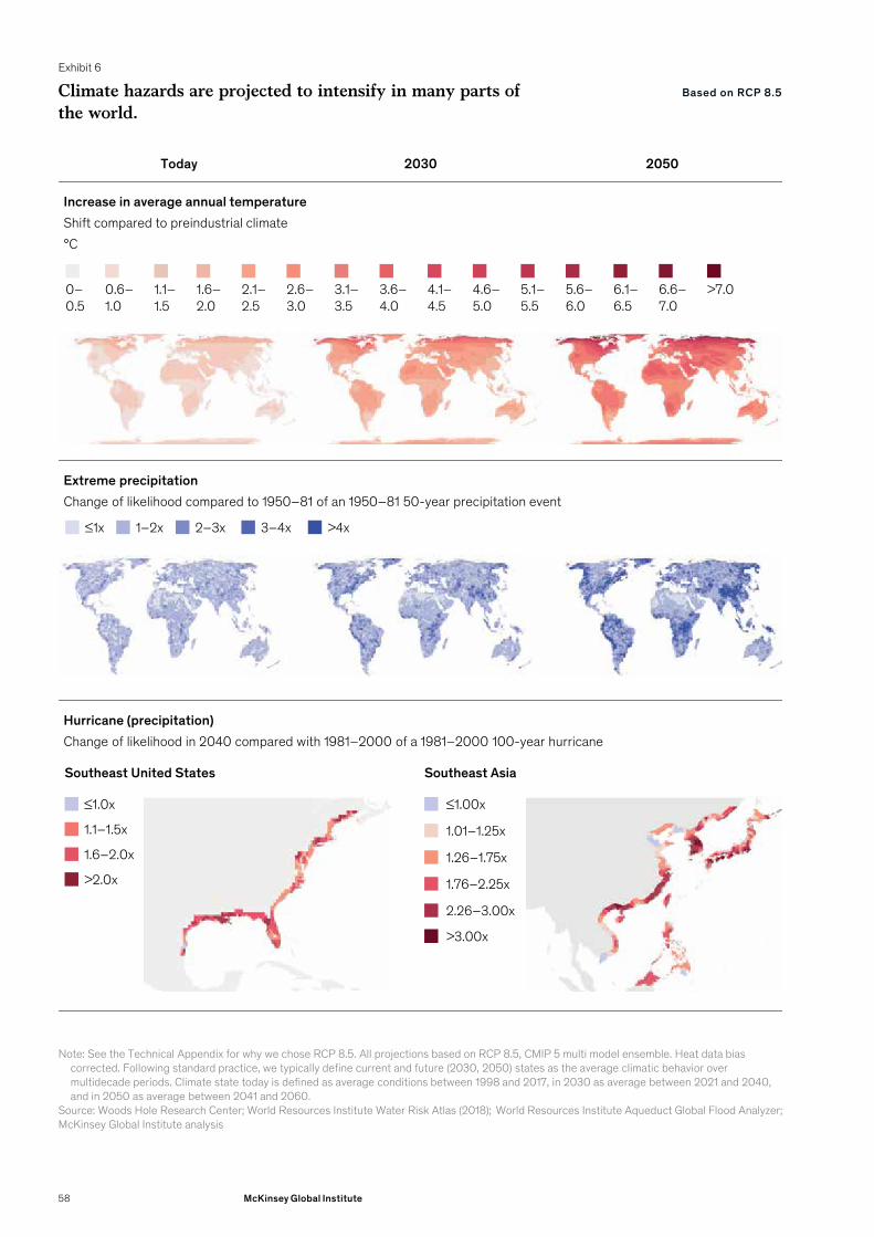
Exhibit 6
Today 2030 2050
Increase in average annual temperatureShift compared to preindustrial climate°C
Extreme precipitationChange of likelihood compared to 1950–81 of an 1950–81 50-year precipitation event
Hurricane (precipitation)Change of likelihood in 2040 compared with 1981–2000 of a 1981–2000 100-year hurricane
Climate hazards are projected to intensify in many parts of the world.
Note: See the Technical Appendix for why we chose RCP 8.5. All projections based on RCP 8.5, CMIP 5 multi model ensemble. Heat data bias corrected. Following standard practice, we typically define current and future (2030, 2050) states as the average climatic behavior over multidecade periods. Climate state today is defined as average conditions between 1998 and 2017, in 2030 as average between 2021 and 2040, and in 2050 as average between 2041 and 2060.
Source: Woods Hole Research Center; World Resources Institute Water Risk Atlas (2018); World Resources Institute Aqueduct Global Flood Analyzer; McKinsey Global Institute analysis
≤1x 1–2x 2–3x 3–4x >4x
≤1.0x
1.1–1.5x
1.6–2.0x
>2.0x
Southeast United States Southeast Asia
≤1.00x
1.01–1.25x
1.26–1.75x
1.76–2.25x
2.26–3.00x
>3.00x
Based on RCP 8.5
0–0.5
0.6–1.0
1.1–1.5
1.6–2.0
2.1–2.5
2.6–3.0
3.1–3.5
3.6–4.0
4.1–4.5
4.6–5.0
5.1–5.5
5.6–6.0
6.1–6.5
6.6–7.0
>7.0
58 McKinsey Global Institute

Exhibit 7
Today 2030 2050
Drought frequency1
% of decade in drought
Lethal heat wave probability2
% p.a.
Water supplyChange in surface water compared with 2018 (%)Boundaries on the map represent water basins
Climate hazards are projected to intensify in many parts of the world (continued).
1. Measured using a three-month rolling average. Drought is defined as a rolling three month period with Average Palmer Drought Severity Index (PDSI) <-2. PDSI is a temperature and precipitation-based drought index calculated based on deviation from historical mean. Values generally range from +4 (extremely wet) to -4 (extremely dry).
2. A lethal heat wave is defined as a three-day period with maximum daily wet-bulb temperatures exceeding 34°C wet-bulb, where wet-bulb temperature is defined as the lowest temperature to which a parcel of air can be cooled by evaporation at constant pressure. This threshold was chosen because the commonly defined heat threshold for human survivability is 35°C wet-bulb, and large cities with significant urban heat island effects could push 34°C wet-bulb heat waves over the 35°C threshold. Under these conditions, a healthy, well-hydrated human being resting in the shade would see core body temperatures rise to lethal levels after roughly 4–5 hours of exposure. These projections are subject to uncertainty related to the future behavior of atmospheric aerosols and urban heat island or cooling island effects.
Note: See the Technical Appendix for why we chose RCP 8.5. All projections based on RCP 8.5, CMIP 5 multi model ensemble. Heat data bias corrected. Following standard practice, we typically define current and future (2030, 2050) states as the average climatic behavior over multidecade periods. Climate state today is defined as average conditions between 1998 and 2017, in 2030 as average between 2021 and 2040, and in 2050 as average between 2041 and 2060.
≤2 3–5 6–10 11–15 16–30 31–45 46–60 >60
>70% decrease
41–70% decrease
20–40% decrease
Nearnormal
20–40% increase
41–70% increase
>70% increase
Source: Woods Hole Research Center; World Resources Institute Water Risk Atlas (2018); World Resources Institute Aqueduct Global Flood Analyzer; McKinsey Global Institute analysis
Based on RCP 8.5
0 1–10 11–20 21–40 41–60 61–80 >80
59Climate risk and response: Physical hazards and socioeconomic impacts

Rising flood waters in Venice. © National Geographic
3. Physical climate risk—a micro view
In this chapter, we examine how climate hazard becomes risk. We use our five-systems framework as a basis for understanding physical climate risk in the near term. We examine nine case studies from around the world to assess risks to specific sectors, locations, and markets. The cases were chosen based on their exposure to the extremes of climate change and their proximity today to key physical and biological thresholds. Each case is specific to a geography and an exposed system, and as such is not representative of an “average” environment or level of risk across the world. As noted, these cases are based on an RCP 8.5 climate scenario. By understanding the impact of climate change in a leading-edge case, we provide a methodology to assess risk in other instances which may experience rising climate change risk in the future.
Our case studies cover each of the five systems we assess to be directly affected by physical climate risk, across geographies and sectors (Exhibit 8). While climate change will have an economic impact across many sectors, our cases highlight the impact on construction, agriculture, finance, fishing, tourism, manufacturing, real estate, and a range of infrastructure-based sectors. The cases include the following:
— For livability and workability, we look at the risk of exposure to extreme heat and humidity in India and what that could mean for that country’s urban population and outdoor-based sectors, as well as at the changing Mediterranean climate and how that could affect sectors such as wine and tourism.
— For food systems, we focus on the likelihood of a multiple-breadbasket failure affecting wheat, corn, rice, and soy, as well as, specifically in Africa, the impact on wheat and coffee production in Ethiopia and cotton and corn production in Mozambique.
— For physical assets, we look at the potential impact of storm surge and tidal flooding on Florida real estate and the extent to which global supply chains, including for semiconductors and rare earths, could be vulnerable to the changing climate.
— For infrastructure services, we examine 17 types of infrastructure assets, including the potential impact on coastal cities such as Bristol in England and Ho Chi Minh City in Vietnam.
— Finally, for natural capital, we examine the potential impacts of glacial melt and runoff in the Hindu Kush region of the Himalayas; what ocean warming and acidification could mean for global fishing and the people whose livelihoods depend on it; as well as potential disturbance to forests, which cover nearly one-third of the world’s land and are key to the way of life for 2.4 billion people.
61Climate risk and response: Physical hazards and socioeconomic impacts
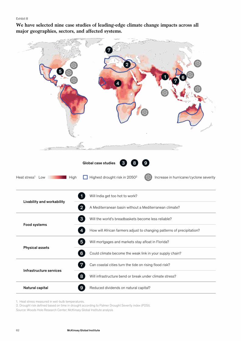
Exhibit 8
We have selected nine case studies of leading-edge climate change impacts across all major geographies, sectors, and affected systems.
Source: Woods Hole Research Center; McKinsey Global Institute analysis
Livability and workabilityWill India get too hot to work?
A Mediterranean basin without a Mediterranean climate?
Food systemsWill the world’s breadbaskets become less reliable?
How will African farmers adjust to changing patterns of precipitation?
Physical assetsWill mortgages and markets stay afloat in Florida?
Could climate become the weak link in your supply chain?
Infrastructure servicesCan coastal cities turn the tide on rising flood risk?
Will infrastructure bend or break under climate stress?
Natural capital Reduced dividends on natural capital?
Highest drought risk in 20502Heat stress1 Low High Increase in hurricane/cyclone severity
1
2
3
4
5
6
7
8
9
3 8 9Global case studies
1. Heat stress measured in wet-bulb temperatures.2. Drought risk defined based on time in drought according to Palmer Drought Severity index (PDSI).
1
2
4
56
7
7
Exhibit 8
62 McKinsey Global Institute
Across our cases, we find climate risk will increase by 2030 and grow further to 2050, often in nonlinear waysAs we noted in Chapter 1, to assess the magnitude of direct physical climate risk in each of the case studies, we examine the severity of the hazard and its likelihood; the exposure of people, assets, or economic activity to the hazard; and the extent to which systems are vulnerable to the hazard. To date, research suggests that the upward trend in economic losses from natural disasters has primarily been driven by an increase in exposure, rather than climate change effects.104 Our case studies provide a window into how that is expected to change. We also assess knock-on impacts from direct risk, for example on GDP or prices, and identify the likely adaptation response and key decisions, implementation challenges, and costs involved in each of our cases.
The insights from our cases help highlight the nature and extent of climate risk. Seven characteristics of physical climate risk stand out. Climate risks are:
— Increasing. In each of our nine cases, the level of climate risk increases by 2030 and further by 2050. Extreme heat and flooding drove the greatest increases in risk across our leading-edge cases of climate change, with increases in socioeconomic impact of between roughly two and 20 times by 2050 versus today’s levels.
— Spatial. Climate hazards manifest locally. The direct impacts of physical climate risk thus need to be understood in the context of a geographically defined area. Absent further adaptation, our research suggests that the nature of flood risks and potential response in Bristol and Ho Chi Minh City could differ, reflecting differences in exposure and severity. Likewise, rising temperatures may initially impact India and the Mediterranean in different ways. In India, it may impact outdoor work and diminish labor productivity while in the Mediterranean it may reduce agricultural yields and tourism. Variations within countries are possible or even likely. For example, the coasts and Indo-Gangetic plains in India are exposed to higher risk of extreme heat and humidity compared with the higher elevation and interior Decca plain, because these regions facilitate the mixing of humid oceanic air with hot and dry continental air. Understanding spatial risk requires understanding both spatial climatic conditions and how exposure and resilience to those climatic conditions vary across geographies.
— Non-stationary. As the Earth continues to warm, physical climate risk is ever-changing or non-stationary. Managing that risk will require not moving to a “new normal” but preparing for a world of constant change. As we discuss elsewhere in this report, probability distributions of temperature continue to shift rightward. Average risk is rising, but tail risk is also increasing. For example, in Florida we find average annual losses for residential real estate due to storm surge damage are $2 billion today and are projected to increase to about $3 billion to $4.5 billion by 2050, with the range depending on whether exposure
104 Various researchers have attempted to identify the role played by each of these factors in driving economic losses to date. Insurance records of losses from acute natural disasters like floods, hurricanes, and forest fires show a clear upward trend in losses in real terms over time, and analyses show that the majority of this is driven by an increase in exposure. This is based on normalizing the real losses for increases in GDP, wealth, and exposure to strip out the effects of a rise in exposure. See for example, Roger Pielke, “Tracking progress on the economic costs of disasters under the indicators of the sustainable development goals,” Environmental Hazards, 2019, Volume 18, Number 1. The work by Pielke finds no upward trend in economic impact after normalizing the damage data, and indeed a decrease in weather /climate losses as a proportion of GDP since 1990. Other researchers find a small upward trend after accounting for effects of GDP, wealth, and population, suggesting some potential role of climate change in losses to date. See for example, Fabian Barthel and Eric Neumayer, “A trend analysis of normalized insured damage from natural disasters,” Climatic Change, 2012, Volume 113, Number 2; and Muir-Wood et al., “The search for trends in a global catalogue of normalized weather-related catastrophe losses,” Climate Change and Disaster Losses Workshop, 2006; Robert Ward and Nicola Ranger, Trends in economic and insured losses from weather-related events: A new analysis, Centre for Climate Change Economics and Policy and Munich Re, November 2010. For example, Muir-Wood et al. conduct analysis of insurance industry data between 1970 to 2005 and find that weather-related catastrophe losses have increased by 2 percent each year since the 1970s, after accounting for changes in wealth, population growth and movement, and inflation (notably, though, in some regions, including Australia, India, and the Philippines, such losses have declined). Analysis by Munich Re finds a statistically significant increase in insured losses from weather-related events in the United States and in Germany over the past approximately 30 to 40 years.
63Climate risk and response: Physical hazards and socioeconomic impacts
is constant or increasing.105 Real estate losses during a 100-year hurricane event in the state are $35 billion today; by 2050, that could rise to $50 billion to $75 billion. In India, the number of people with a non-zero probability of experiencing a lethal heat wave is effectively zero today and projected to be 160 million to 200 million by 2030 (of which 80 million to 120 million are estimated not to have air-conditioned homes) and 310 million to 480 million by 2050 (of which effectively all are likely to have air-conditioned homes by that time).
— Nonlinear. Climate risk can have nonlinear increases in impacts. As climate hazards intensify and become more frequent, our analysis suggests a substantial increase in risk. Physical systems, including physiological, human-made and ecological, have either evolved or been designed to operate within certain climate parameters (Exhibit 9). Even small changes in climate hazard can therefore have significant impact if physical thresholds for resilience are breached. Inherent risk is high when regions are already close to systemic thresholds for climate hazards. For example, some parts of India are close to crossing temperature thresholds that would make outdoor work extremely challenging. As of 2017, heat-exposed work produced about 50 percent of GDP, drove about 30 percent of GDP growth, and employed about 75 percent of the labor force, some 380 million people.106
The human body provides one example of physical thresholds and the nonlinear effect if those thresholds are breached. It must maintain a relatively stable core temperature of approximately 37 degrees Celsius to function properly. The core temperature needs to rise only 0.2 degree to compromise multitasking ability, 0.9 degree to compromise neuromuscular coordination, 1.3 degrees to affect simple mental performance, 3 degrees to induce dangerous heatstroke, and 5 degrees to cause death.107 In environments where air temperatures are higher than core body temperature, the body loses its ability to dissipate heat through radiation and convection. Core temperature is determined primarily by a combination of activity level and wet-bulb temperature—a measure of air temperature and relative humidity—that determines how much heat the body can exhaust through the evaporation of sweat. At a wet-bulb temperature of 35 degrees Celsius, healthy, well-hydrated human beings resting in the shade would see core temperatures rise to lethal levels after roughly four to five hours of exposure.108 Labor capacity would be impaired at wet-bulb temperatures well below that.
Other examples include corn, which has a plant physiological threshold at about 20 degrees Celsius, beyond which yields decline dramatically. Human-made assets like power infrastructure and cell phone towers have been designed with certain tolerances for heat, wind, and flooding. Intensifying hazards could thus lead such infrastructure assets to fail with increasing frequency. During Hurricane Maria in 2018, for example, winds of up to 280 km/h felled more than 90 percent of the cell phone towers in Puerto Rico.109
105 Analysis conducted by KatRisk; direct average annual losses to all residential real estate (insured and uninsured properties). This is the long-term average loss expected in any one year, calculated by modeling the probability of a climate hazard occurring multiplied by the damage should that hazard occur, and summing over events of all probabilities. Analyses based on sea level rise in line with the US Army Corps of Engineers high curve, one of the recommended curves from the Southeast Florida Regional Climate Change Compact. Southeast Florida Regional Climate Change Compact Sea Level Rise Work Group, Unified sea level rise projection: Southeast Florida, October 2015.
106 Reserve Bank of India, Database on Indian Economy, dbie.rbi.org.in/DBIE/dbie.rbi?site=home. Exposed sectors include exclusively outdoor sectors such as agriculture, mining, and quarrying, as well as indoor sectors with poor air-conditioning penetration, including manufacturing, hospitality, and transport.
107 P. A. Hancock and Ioannis Vasmatzidis, “Human occupational and performance limits under stress: The thermal environment as a prototypical example,” Ergonomics, 1998, Volume 41, Number 8.
108 Steven C. Sherwood and Matthew Huber, “An adaptability limit to climate change due to heat stress,” Proceedings of the National Academy of Sciences, May 25, 2010, Volume 107, Number 21; threshold confirmed, assuming light clothing cover, using the physiological Predicted Heat Strain (PHS) model; Jacques Malchaire et al., “Development and validation of the predicted heat strain model,” Annals of Occupational Hygiene, March 2001, Volume 45, Number 2.
109 The 2017 Atlantic Hurricane Season: Mobile industry impact and response in the Caribbean, GSMA.
64 McKinsey Global Institute
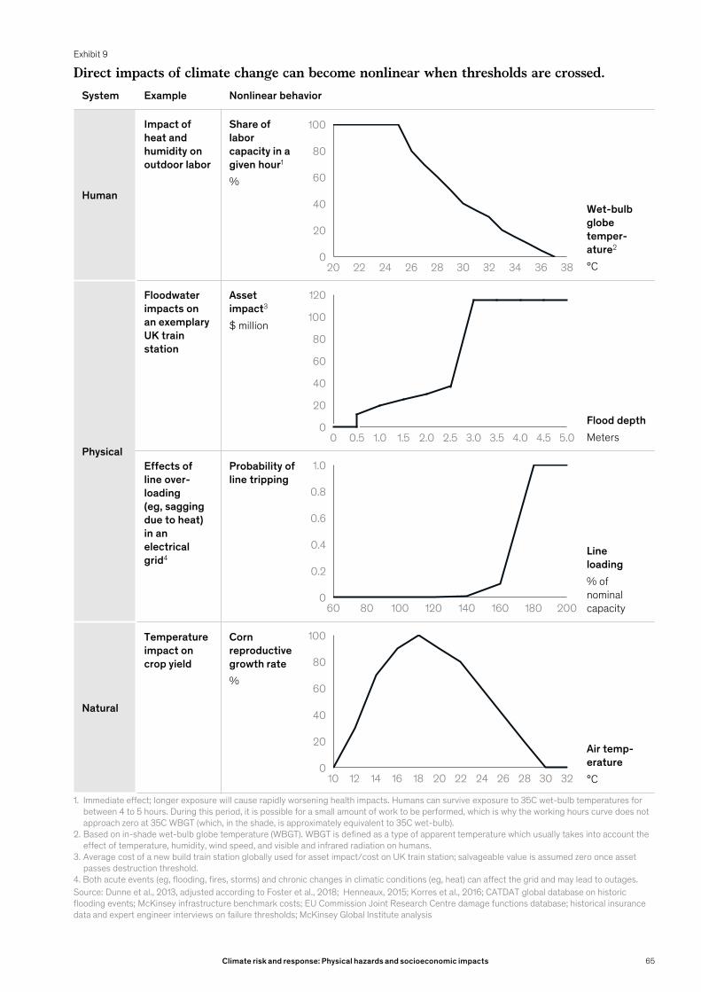
Exhibit 9
System Example Nonlinear behavior
Human
Impact of heat and humidity on outdoor labor
Share of labor capacity in a given hour1
%
Wet-bulb globe temper-ature2
°C
Physical
Floodwater impacts on an exemplary UK train station
Asset impact3
$ million
Flood depthMeters
Effects of line over-loading (eg, sagging due to heat) in an electrical grid4
Probability of line tripping
Line loading% of nominal capacity
Natural
Temperature impact on crop yield
Corn reproductive growth rate%
Air temp-erature°C
Direct impacts of climate change can become nonlinear when thresholds are crossed.
Source: Dunne et al., 2013, adjusted according to Foster et al., 2018; Henneaux, 2015; Korres et al., 2016; CATDAT global database on historic flooding events; McKinsey infrastructure benchmark costs; EU Commission Joint Research Centre damage functions database; historical insurance data and expert engineer interviews on failure thresholds; McKinsey Global Institute analysis
1. Immediate effect; longer exposure will cause rapidly worsening health impacts. Humans can survive exposure to 35C wet-bulb temperatures for between 4 to 5 hours. During this period, it is possible for a small amount of work to be performed, which is why the working hours curve does not approach zero at 35C WBGT (which, in the shade, is approximately equivalent to 35C wet-bulb).
2. Based on in-shade wet-bulb globe temperature (WBGT). WBGT is defined as a type of apparent temperature which usually takes into account the effect of temperature, humidity, wind speed, and visible and infrared radiation on humans.
3. Average cost of a new build train station globally used for asset impact/cost on UK train station; salvageable value is assumed zero once asset passes destruction threshold.
4. Both acute events (eg, flooding, fires, storms) and chronic changes in climatic conditions (eg, heat) can affect the grid and may lead to outages.
100
3422 3020 28 3824 26 32 360
20
40
60
80
160 20060 180
0.8
80
0.6
1401201000
0.2
0.4
1.0
10 1612 14
60
18 20 22
100
24 26 28 30 320
20
40
80
3.52.00 1.00.5 1.5 2.5 3.0 4.0
40
4.5 5.00
20
120
60
80
100
65Climate risk and response: Physical hazards and socioeconomic impacts

Extreme heat is already disrupting global air travel. In July 2017, for example, about 50 flights out of Phoenix, Arizona, were grounded for physical and regulatory reasons when temperatures rose to 48 degrees Celsius.110 We find the disruption could increase; by 2050, as many as 185,000 passengers per year could be affected by flights that are grounded because of extreme heat, according to our estimates.
The thresholds we describe above pertain to physical systems. The economic, financial, and social systems that rely on these physical systems also have thresholds, which are harder to quantify. Nonetheless, intensifying direct impacts of climate change could trigger nonlinear responses in those systems, too. For example, there could be psychological thresholds for home buyers, for when the flooding frequency of homes changes from being merely “inconvenient” to “intolerable.” Financial markets, too, may hit a point at which they limit long-term lending to risky geographies. Some intensifying hazards could even trigger widespread internal or external displacement of people. As CO2 concentrations rise and the climate changes, natural systems may not be able to evolve fast enough to keep pace, requiring a targeted focus on adaptation action to build resilience and prevent such nonlinear responses.
— Systemic. While the direct impact from physical climate risk is local, it can have knock-on effects across regions and sectors, through interconnected socioeconomic systems. We find that knock-on impacts could be especially large when people and assets that are affected are central to local economies and those local economies are tied into other economic and financial systems. Florida’s economy, for example, relies on real estate, with 22 percent of GDP, 30 percent of local tax revenue, and home owner wealth linked to the sector (primary residences represent 42 percent of median home owner wealth in the United States).111 Flooding in the state could thus not only damage housing but also affect property values of exposed homes, in turn reducing property tax revenues and potentially affecting future price or availability of insurance. We estimate that devaluation of flood-exposed homes in Florida could total $10 billion to $30 billion by 2030, all else being equal.
— Regressive. Climate risk is regressive. The poorest communities and populations within each of our cases are often the most exposed to climate risk, for example, those dependent on outdoor work in areas of increasing heat duress. They are often the most vulnerable, lacking financial means. For example, in the case of a multiple breadbasket failure, a yield failure in two or more key production regions for rice, wheat, corn, and soy, we estimate that prices could spike by 100 percent or more in the short term. This would particularly hurt the poorest communities, including the 750 million people living below the international poverty line. Climate risk creates spatial inequality, as it may simultaneously benefit some regions while hurting others. Rising temperatures may boost tourism in areas of northern Europe while reducing the economic vitality of southern ones, for example. The volume of water in basins in northern Africa, Greece, and Spain could decline by more than 15 percent by 2050 even as the volume in basins in Germany and the Netherlands increases by 1 to 5 percent, in turn affecting agriculture such as wine and tomatoes.
110 Regulators only certify planes to fly below certain temperatures. As air temperature rises, the density of the air decreases and negatively affects lift. As a result, planes require a combination of more thrust, lighter takeoff weights, and longer runways to take off. See Rhett Allain, “Why Phoenix’s airplanes can’t take off in extreme heat,” Wired, June 20, 2017.
111 National Association of Realtors, The economic impact of a typical home sale in Florida, 2018; other income sources are value-added taxes, fees, and business revenues. For more details, see Household wealth & real estate, UPFINA, September 2018; Federal Reserve Bank of St. Louis, FRED database, Homeownership rate for Florida, fred.stlouisfed.org/series/FLHOWN; Michael Neal, “Housing remains a key component of household wealth,” Eye on Housing, National Association of Home Builders, September 4, 2013.
66 McKinsey Global Institute

— Under-prepared. While companies and communities have been adapting to reduce climate risk, the pace and scale of adaptation may need to increase significantly to manage rising levels of physical climate risk. Adaptation can be challenging, as it can entail rising costs and tough choices. These could include whether to invest in hardening or to relocate people and assets. Adaptation will likely also require coordinated action across multiple stakeholders, although this varies across cases. For semiconductor plants, effective adaptation might be feasible in a comparatively cost-effective manner through either asset hardening or insurance. Due to hazard intensity increasing, the economics of adaptation will likely worsen over time, and there may eventually be technical or other limits to effective adaptation. In some parts of Florida, the cost of building new sea walls and other protection from flooding hazards might increase over time and prove technically challenging. If that is the case, hard choices will need to be made between spending on hardening or relocation. In other cases, such as warming oceans that reduce the fish stocks that fishing communities rely on, collective action may be needed, making the path to adaptation more challenging. In some cases, local economic conditions may make financing difficult.
Livability and workability: Parts of India could become intolerably hot and humid, while in the Mediterranean, agriculture and tourism may be affectedIn India, the impact of extreme heat and humidity may be underappreciated today as communities grapple with issues of air quality and water stress. Conditions in the country are already relatively hot and humid, but rising heat and humidity resulting from the changing climate could push conditions over physiological thresholds for livability and workability, in particular for already-vulnerable parts of the population. This will threaten the lives of millions of people and make outdoor work, which accounts for about half of GDP today, far more challenging.
Climate models we draw on predict that under an RCP 8.5 scenario, India may become one of the first places in the world to experience heat waves that cross the survivability threshold for a healthy human being resting in the shade.112 By 2030, some 160 million to 200 million people (of whom 80 million to 120 million people are estimated not to have air-conditioned homes) are expected to live in urban areas with a non-zero probability of such heat waves occurring. This could rise to between 310 million and 480 million by 2050, without factoring in air conditioner penetration, which at current rates of growth could rise to cover the full population by that time.113 Most of this population is projected to live in regions with a roughly 5 percent average annual probability of experiencing a lethal heat wave by 2030, and as much as 14 percent by 2050 (Exhibit 10). This means that the average person living in an at-risk region has a probability of roughly 40 percent of experiencing a lethal heat wave at least once in the decade centered on 2030. In the decade centered on 2050, that probability could rise to roughly 80 percent.114
112 Researchers have established the survivability threshold as wet-bulb temperatures that exceed 35°C for more than five hours. Steven C. Sherwood and Matthew Huber, “An adaptability limit to climate change due to heat stress,” Proceedings of the National Academy of Sciences, May 25, 2010, Volume 107, Number 21.
113 Range is based on the range of population projections from the UN World Population Prospects and the UN World Urbanization Prospects, to bound population growth based on high and low variants, and based on urban and total population growth rates.
114 Note that if atmospheric aerosol concentration does not decrease over the next decade, the probability of lethal heat waves could be reduced, as atmospheric aerosols (particularly black carbon) are not currently appropriately represented in the CMIP5 ensemble Global Climate Models. See India case for more details.
67Climate risk and response: Physical hazards and socioeconomic impacts
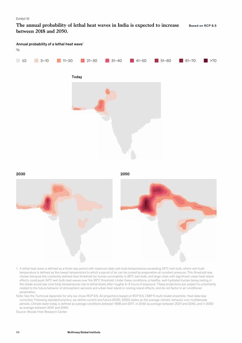
Exhibit 10
The annual probability of lethal heat waves in India is expected to increase between 2018 and 2050.
Source: Woods Hole Research Center
1. A lethal heat wave is defined as a three-day period with maximum daily wet-bulb temperatures exceeding 34°C wet-bulb, where wet-bulb temperature is defined as the lowest temperature to which a parcel of air can be cooled by evaporation at constant pressure. This threshold was chosen because the commonly defined heat threshold for human survivability is 35°C wet-bulb, and large cities with significant urban heat island effects could push 34°C wet-bulb heat waves over the 35°C threshold. Under these conditions, a healthy, well-hydrated human being resting in the shade would see core body temperatures rise to lethal levels after roughly 4–5 hours of exposure. These projections are subject to uncertainty related to the future behavior of atmospheric aerosols and urban heat island or cooling island effects, and do not factor in air conditioner penetration.
Note: See the Technical Appendix for why we chose RCP 8.5. All projections based on RCP 8.5, CMIP 5 multi model ensemble. Heat data bias corrected. Following standard practice, we define current and future (2030, 2050) states as the average climatic behavior over multidecade periods. Climate state today is defined as average conditions between 1998 and 2017, in 2030 as average between 2021 and 2040, and in 2050 as average between 2041 and 2060.
Today
2030 2050
Annual probability of a lethal heat wave1
%
3–10 11–20 21–30 31–40 41–50 51–60 61–70≤2 >70
Based on RCP 8.5
68 McKinsey Global Institute

As heat and humidity increase, this also could affect labor productivity in outdoor work, as workers will need to take breaks to avoid heatstroke. Moreover, their bodies will protectively fatigue, in a so-called self-limiting process, to avoid overheating. We estimate that the effective number of outdoor daylight hours lost in an average year because of diminished labor productivity would increase by about 15 percent by 2030 compared with today, equivalent to an additional four weeks of work from 11 a.m. to 4 p.m. lost, assuming a 12-hour workday.115 This would likely cause a reduction in GDP of between 2.5 and 4.5 percent by 2030, where the range is based on the 25th and 75th percentile climate model ensemble projections (Exhibit 11).116 By 2050, it is expected that some parts of India will be under such intense heat and humidity duress that working outside would effectively not be feasible for almost 30 percent of annual daylight hours. The urban poor without access to cooling systems and those engaged in outdoor activities like agriculture and construction will be among the vulnerable who are disproportionately affected.
India, however, has potential for adaptation in the short term. Steps include early-warning systems and cooling shelters to protect those without air-conditioning. Working hours for outdoor workers could be shifted, and cities could implement albedo heat-management efforts. At the extreme, coordinated movement of people and capital from high-risk areas could be organized. Beyond the costs involved, adaptation could be challenging if it changes how people conduct their daily lives or requires them to move to less at-risk areas.
Rising temperatures would also affect the Mediterranean, albeit with less severe impacts than in India. The mild Mediterranean climate will grow hotter, which could disrupt key industries such as tourism and agriculture. By 2050, drought conditions are expected to prevail for at least six months of every year (Exhibit 12).117 Even under a conservative scenario of reduced emissions, Madrid’s climate in 2050 is projected to resemble today’s climate in Marrakech, while the climate in Marseille in 2050 may be like that of Algiers today.118 Climate scientists expect an increase in the number of days considered uncomfortably hot in many Mediterranean beach tourism locations, while northern European coasts could become more agreeable as summer holiday destinations. This could change visitor flows and exacerbate spatial inequality.119 Farmers have already seen their crop yields diminish and become less predictable, a trend that is likely to continue.120 Areas known for the quality of their wine grapes risk losing their prominence on the viticulture map, while nontraditional growing regions may gain advantage.
Adaption will need to be place-based, given the strong ties to location of agriculture and tourism. For example, wineries could harvest earlier, reduce sunlight on grapes, or irrigate vineyards. Additionally, approaches such as modified fertilizer use and planting resilient varieties of crops might mitigate decreases in yield.121 Tourism destinations at risk from rising summer temperatures might explore ways to shift visitor flows to shoulder seasons and diversify local economies.
115 An average year is defined as the ensemble mean projection across the 2012–40 period. 116 Lost working hours calculated according to the methodology of John P. Dunne et al., “Reductions in labour capacity from
heat stress under climate warming,” Nature Climate Change, February 2013, Volume 3, but corrected using empirical data from Josh Foster et al., “A New Paradigm To Quantify The Reduction Of Physical Work Capacity In The Heat,” Medicine and Science in Sports and Exercise, June 2019, Volume 51, Issue 6.
117 A month in drought is defined as a month with Palmer Drought Severity index < -2. The index is a temperature and precipitation-based metric calculated based on deviation from historical mean. Values range from +4 (extremely wet) to -4 (extremely dry).
118 This is considering an RCP 4.5 emissions pathway scenario. Jean-Francois Bastin et al., “Understanding climate change from a global analysis of city analogues,” PLOS ONE, July 2019, Volume 14, Number 7.
119 We use 37 degrees Celsius as the temperature at which days start to feel “too hot.” The actual threshold varies by individual.
120 Deepak K. Ray et al., “Climate change has likely already affected global food production,” PLoS ONE, May 2019, Volume 14, Issue 5.
121 Our analysis does not account for the potential migration of planting areas for a crop within a country. For farmers who can change what they grow, this can create opportunities. For example, a high-latitude country like Canada could have significantly increased agricultural opportunities due to climate change. But in many countries, as the crop-growing regions shift, farmers may not be able to adapt.
69Climate risk and response: Physical hazards and socioeconomic impacts
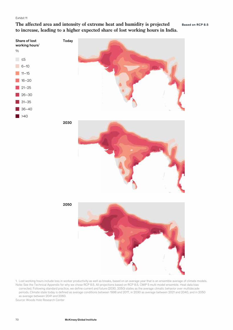
Exhibit 11
The affected area and intensity of extreme heat and humidity is projected to increase, leading to a higher expected share of lost working hours in India.
Source: Woods Hole Research Center
1. Lost working hours include loss in worker productivity as well as breaks, based on an average year that is an ensemble average of climate models. Note: See the Technical Appendix for why we chose RCP 8.5. All projections based on RCP 8.5, CMIP 5 multi model ensemble. Heat data bias
corrected. Following standard practice, we define current and future (2030, 2050) states as the average climatic behavior over multidecade periods. Climate state today is defined as average conditions between 1998 and 2017, in 2030 as average between 2021 and 2040, and in 2050 as average between 2041 and 2060.
Today
2030
2050
Share of lost working hours1
%
6–10
11–15
16–20
21–25
26–30
31–35
36–40
≤5
>40
Based on RCP 8.5
70 McKinsey Global Institute
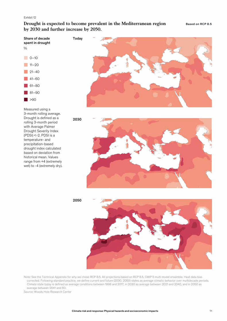
Exhibit 12
Drought is expected to become prevalent in the Mediterranean region by 2030 and further increase by 2050.
Source: Woods Hole Research Center
Note: See the Technical Appendix for why we chose RCP 8.5. All projections based on RCP 8.5, CMIP 5 multi model ensemble. Heat data bias corrected. Following standard practice, we define current and future (2030, 2050) states as average climatic behavior over multidecade periods. Climate state today is defined as average conditions between 1998 and 2017, in 2030 as average between 2021 and 2040, and in 2050 as average between 2041 and 60.
Share of decade spent in drought%
0–10
11–20
21–40
41–60
61–80
81–90
>90
Today
2030
2050
Measured using a 3-month rolling average. Drought is defined as a rolling 3-month period with Average Palmer Drought Severity Index (PDSI) <-2. PDSI is a temperature- and precipitation-based drought index calculated based on deviation from historical mean. Values range from +4 (extremely wet) to -4 (extremely dry).
Based on RCP 8.5
71Climate risk and response: Physical hazards and socioeconomic impacts
Food systems: A global yield shock is projected to become more likely, while African countries may experience shifts in their agricultural endowmentWe find an increasing risk of a concurrent harvest failure in multiple breadbasket locations, an example of a tail event. We define a multiple breadbasket failure as a global harvest decline of 15 percent relative to average.122 About 60 percent of global grain production today occurs in just five regional breadbaskets, and four grains make up almost half of the calories in the average global diet (Exhibit 13). Rising temperatures, changing patterns of precipitation, and increasing episodes of climate-related stress such as drought, heat waves, and floods are expected to raise the likelihood of a multiple-breadbasket failure in the decades ahead. However, it is also important to note that some countries are projected to benefit and experience rising yields due to climate change; we discuss this further in Chapter 4.123
We estimate that the chance of a greater than 15 percent yield shock at least once in the decade centered on 2030 rises from 10 percent today to 18 percent, while the chance of a greater than 10 percent yield shock occurring at least once rises from 46 to 69 percent (Exhibit 14).124 Since there is a built-up stock of grain (current stock-to-use ratios are high, at 30 percent of consumption), such a yield shock would most likely not directly lead to food shortages. It is highly unlikely that the world will run out of grain within any one year. However, even limited reductions in stock-to-use ratios have triggered episodes of food price spikes. A 15 percent drop in global supply, for example, would likely cause stock-to-use ratios to drop to about 20 percent. In that case, historical precedent suggests that prices could spike by 100 percent or more in the short term, although we acknowledge that food commodity prices are difficult to predict. If such a food price spike were to occur, this would particularly hurt poor people worldwide, including the 750 million people living below the international poverty line.
To make the food system more resilient, private and public research could be expanded. For instance, research on technologies could aim to make crops more resistant to abiotic and biotic stresses. This may include conventional breeding, gene editing, and other biological or physical approaches. To offset the risk of a harvest failure of greater than 15 percent, the current global stock-to-use ratio could be increased to 35 to 40 percent, leveraging times of surplus and low prices. We estimate total costs for the required additional storage at between $5 billion and $11 billion per year. Investment in water management systems is another potential adaptation measure. Incentives for farmers, however, are not aligned with stock buildup. Storing grain can be expensive (given direct costs as well as working capital requirements), and the reduced risk of food shortages is to some extent a positive externality that farmers do not necessarily factor into their cost-benefit analysis. Multilateral organizations such as the Food and Agriculture Organization of the United Nations could potentially play a role, managing storage closely to prevent “leakages” and encouraging the private sector to store more grains. In any case, affected stakeholders may need to work together to solve storage issues, possibly through global interventions.
122 We define a breadbasket as a key production region for food grains (rice, wheat, corn, and soy) and harvest failure as a major yield reduction in the annual crop cycle of a breadbasket region where there is a potential impact on the global food system. Note that we are taking into account potentially positive effects on plant growth from higher CO2 levels (“CO2 fertilization”). However, those benefits could be reduced as increased CO2 levels could lead to a reduction in the protein and micronutrient content of crops, which in turn would require humans to eat more volume to achieve the same level of nutrition. For more detail, see Chunwu Zhu et al., “Carbon dioxide (CO2) levels this century will alter the protein, micronutrients, and vitamin content of rice grains with potential health consequences for the poorest rice-dependent countries,” Science Advances, May 23, 2018, Volume 4, Number 5.
123 For this case, we modeled only the impact of changes in temperature and precipitation on yields. We did not model extreme events (such as flooding, hail, or extreme wind) nor the impact of pests and diseases.
124 See the breadbasket case study for details.
72 McKinsey Global Institute
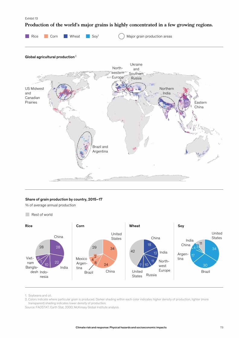
Exhibit 13
Production of the world’s major grains is highly concentrated in a few growing regions.
Source: FAOSTAT; Earth Stat, 2000; McKinsey Global Institute analysis
1. Soybeans and oil.2. Colors indicate where particular grain is produced. Darker shading within each color indicates higher density of production, lighter (more
transparent) shading indicates lower density of production.
Rice Corn Wheat Soy1 Major grain production areas
Global agricultural production 2
Brazil and Argentina
US Midwest and Canadian Prairies
North-western Europe
Ukraine and
Southern Russia
Eastern China
Northern India
Share of grain production by country, 2015–17% of average annual production
34
248
29
Argen-tina
24
China
UnitedStates
Mexico
Brazil
18
12
11107
42
China
UnitedStates
India
North-westEurope
Russia
34
30
17
11
Argen-tina
UnitedStates
34
Brazil
ChinaIndia
28
22107
6
28
China
IndiaIndo-nesia
Bangla-desh
Viet-nam
Corn Wheat SoyRice
Rest of world
73Climate risk and response: Physical hazards and socioeconomic impacts
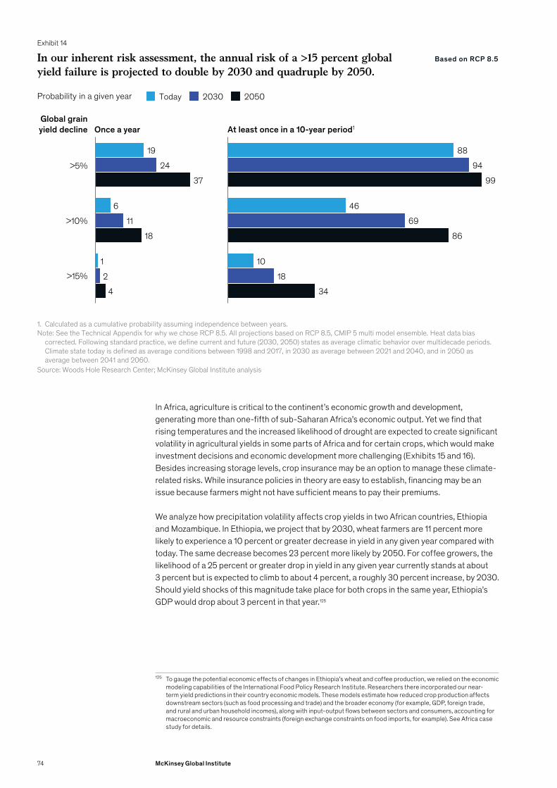
In Africa, agriculture is critical to the continent’s economic growth and development, generating more than one-fifth of sub-Saharan Africa’s economic output. Yet we find that rising temperatures and the increased likelihood of drought are expected to create significant volatility in agricultural yields in some parts of Africa and for certain crops, which would make investment decisions and economic development more challenging (Exhibits 15 and 16). Besides increasing storage levels, crop insurance may be an option to manage these climate-related risks. While insurance policies in theory are easy to establish, financing may be an issue because farmers might not have sufficient means to pay their premiums.
We analyze how precipitation volatility affects crop yields in two African countries, Ethiopia and Mozambique. In Ethiopia, we project that by 2030, wheat farmers are 11 percent more likely to experience a 10 percent or greater decrease in yield in any given year compared with today. The same decrease becomes 23 percent more likely by 2050. For coffee growers, the likelihood of a 25 percent or greater drop in yield in any given year currently stands at about 3 percent but is expected to climb to about 4 percent, a roughly 30 percent increase, by 2030. Should yield shocks of this magnitude take place for both crops in the same year, Ethiopia’s GDP would drop about 3 percent in that year.125
125 To gauge the potential economic effects of changes in Ethiopia’s wheat and coffee production, we relied on the economic modeling capabilities of the International Food Policy Research Institute. Researchers there incorporated our near-term yield predictions in their country economic models. These models estimate how reduced crop production affects downstream sectors (such as food processing and trade) and the broader economy (for example, GDP, foreign trade, and rural and urban household incomes), along with input-output flows between sectors and consumers, accounting for macroeconomic and resource constraints (foreign exchange constraints on food imports, for example). See Africa case study for details.
Exhibit 14
Global grain yield decline Once a year At least once in a 10-year period1
>5%
>10%
>15%
Source: Woods Hole Research Center; McKinsey Global Institute analysis
1. Calculated as a cumulative probability assuming independence between years.Note: See the Technical Appendix for why we chose RCP 8.5. All projections based on RCP 8.5, CMIP 5 multi model ensemble. Heat data bias
corrected. Following standard practice, we define current and future (2030, 2050) states as average climatic behavior over multidecade periods. Climate state today is defined as average conditions between 1998 and 2017, in 2030 as average between 2021 and 2040, and in 2050 as average between 2041 and 2060.
In our inherent risk assessment, the annual risk of a >15 percent global yield failure is projected to double by 2030 and quadruple by 2050.
Today 2030 2050Probability in a given year
19
6
1
24
11
2
37
18
4
88
46
10
94
69
18
99
86
34
Based on RCP 8.5
74 McKinsey Global Institute
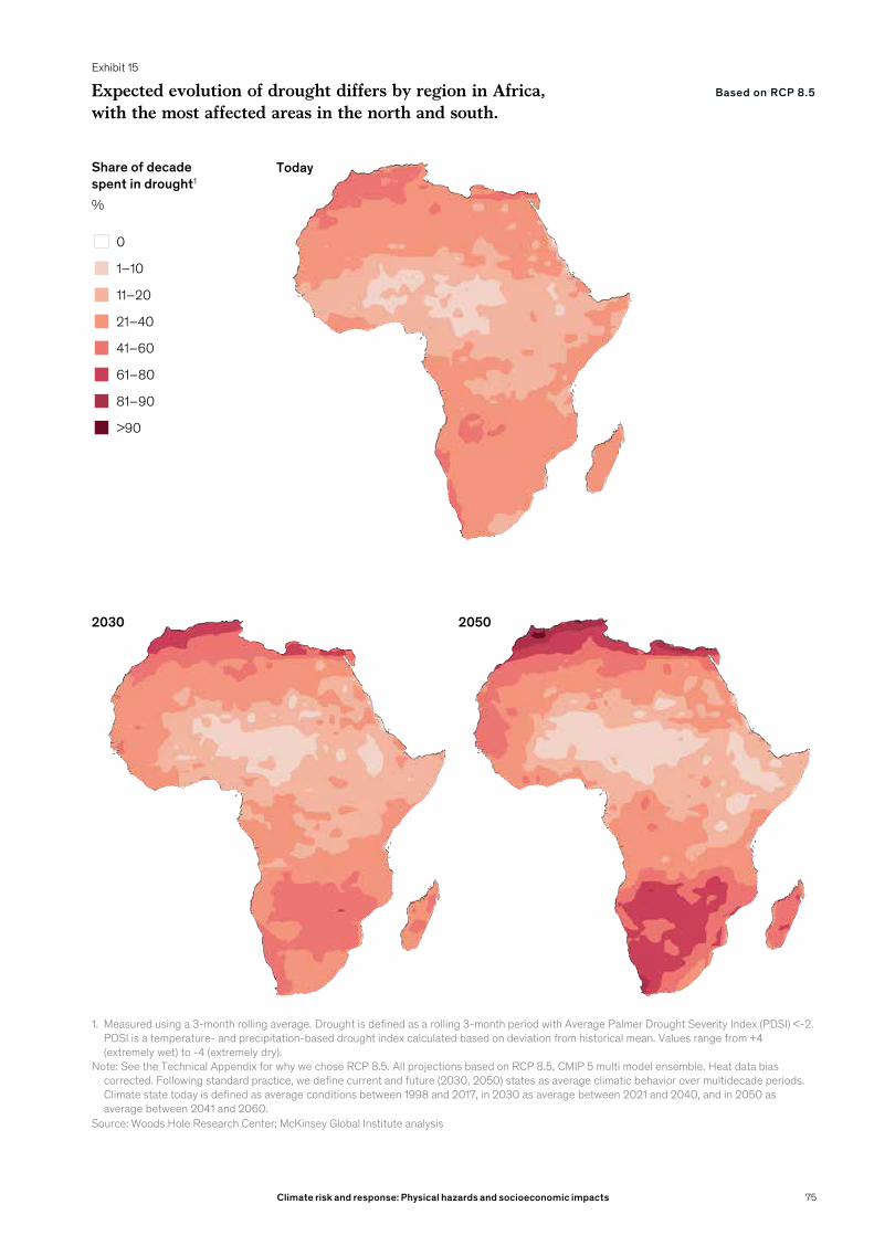
Exhibit 15
Expected evolution of drought differs by region in Africa, with the most affected areas in the north and south.
Source: Woods Hole Research Center; McKinsey Global Institute analysis
1. Measured using a 3-month rolling average. Drought is defined as a rolling 3-month period with Average Palmer Drought Severity Index (PDSI) <-2. PDSI is a temperature- and precipitation-based drought index calculated based on deviation from historical mean. Values range from +4 (extremely wet) to -4 (extremely dry).
Note: See the Technical Appendix for why we chose RCP 8.5. All projections based on RCP 8.5, CMIP 5 multi model ensemble. Heat data bias corrected. Following standard practice, we define current and future (2030, 2050) states as average climatic behavior over multidecade periods. Climate state today is defined as average conditions between 1998 and 2017, in 2030 as average between 2021 and 2040, and in 2050 as average between 2041 and 2060.
Share of decade spent in drought1
%
0
1–10
11–20
21–40
41–60
61–80
81–90
>90
Today
2030 2050
Based on RCP 8.5
75Climate risk and response: Physical hazards and socioeconomic impacts
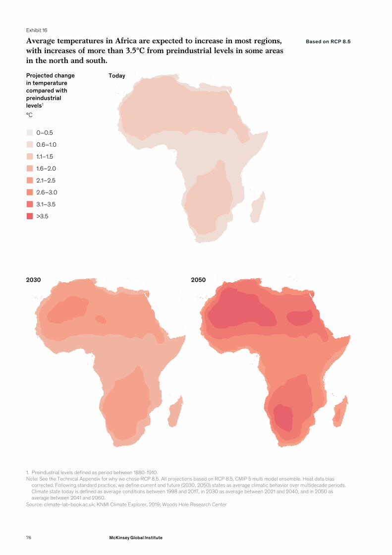
Exhibit 16
Average temperatures in Africa are expected to increase in most regions, with increases of more than 3.5°C from preindustrial levels in some areas in the north and south.
Source: climate-lab-book.ac.uk; KNMI Climate Explorer, 2019; Woods Hole Research Center
1. Preindustrial levels defined as period between 1880-1910.Note: See the Technical Appendix for why we chose RCP 8.5. All projections based on RCP 8.5, CMIP 5 multi model ensemble. Heat data bias
corrected. Following standard practice, we define current and future (2030, 2050) states as average climatic behavior over multidecade periods. Climate state today is defined as average conditions between 1998 and 2017, in 2030 as average between 2021 and 2040, and in 2050 as average between 2041 and 2060.
Projected change in temperature compared with preindustrial levels1
°C
Today
2030 2050
0–0.5
0.6–1.0
1.1–1.5
1.6–2.0
2.1–2.5
2.6–3.0
3.1–3.5
>3.5
Based on RCP 8.5
76 McKinsey Global Institute
In Mozambique, two of the most important crops are corn (maize), which is grown primarily as a food crop, and cotton, which is raised primarily as a cash crop for export. Our analysis suggests that the changing climate will make corn yields more volatile and have the opposite effect on cotton, which typically prefers hotter temperatures. In the case of corn, the likelihood of a large seasonal crop loss (exceeding 30 percent) is currently near zero. By 2030, we project that such a loss will have a 2 percent likelihood of occurring in a given year. However, our projections also indicate that the likelihood of unusually high yields (20 to 30 percent greater than normal) will also increase.126 Cotton growers in Mozambique, by contrast, are projected to experience more stability in yields and thus to benefit from the effects of climate change. We project that a 20 percent or greater drop in yields, compared with average yields, will be 95 percent less likely in 2030 than it was between 1990 and now. Barring other influences, like changes in pests, this reduction in volatility should help the many rural households that rely on cotton crops for much of their income (overall, cotton contributes about one-fifth of Mozambique’s agricultural export earnings).
Physical assets: Increased flooding in Florida could have financial costs beyond physical damages. For supply-chains, rising risk of disruption may require hardening production sites and raising inventoriesIn Florida, expected direct physical damages to real estate are expected to grow with the changing climate, but financial knock-on effects could be even greater. Storm surge from hurricanes is projected to become more severe and tidal flooding more frequent.127 The geography of the state—an expansive coastline, low elevation, and a porous limestone foundation—makes it vulnerable to flooding and makes adaptation challenging. Rising sea levels could push saltwater into the freshwater supply and damage water management systems. Climate hazards will likely have a direct impact on home owners as well as significant knock-on effects on the state’s economy more broadly.
With increasing hurricane intensity and rising sea levels, tail events are likely to cause more impact and become more likely than they are today. Florida’s real estate losses during storm surge from a 100-year hurricane event would be $35 billion today, which are forecast to grow to $50 billion by 2050, assuming no change in building stock (Exhibit 17).128. Real estate is both a physical and a financial store of value for most economies. Damages and the expectation of future damages to homes and infrastructure could drive down prices of exposed homes. The state’s assets and people and its economic activity tend to be concentrated in coastal areas exposed to these hazards. Based on historical trends on the impacts of frequent tidal flooding, devaluation of exposed homes could be $10 billion to $30 billion in 2030 and $30 billion to $80 billion in 2050, all else being equal.129 This corresponds to about a 15 to 35 percent impact. The devaluation could be significantly larger if climate hazards affect public infrastructure assets like water, sewage, and transportation systems, or if home owners more deliberately factor climate risk into their buying decisions. For example, rough estimates suggest that the price effects discussed above could impact property tax revenue in some of the most affected counties by about 15 to 30 percent (though impacts across the state could be less, at about 2 to 5 percent).
126 Although the country’s overall corn production is projected to become more volatile, the impacts we modeled for corn crops obscure the possibility that impacts could differ from one area to another. Subnational predictions for agro-ecological zones will better inform country planning.
127 Thomas Knutson et al., Tropical cyclones and climate change assessment: Part II. Projected response to anthropogenic warming, American Meteorological Society, 2019. Kristina A. Dahl, Melanie F. Fitzpatrick, Erika Spanger-Siegfried, “Sea level rise drives increased tidal flooding frequency at tide gauges along the U.S. East and Gulf Coasts: Projections for 2030 and 2045,” PLoS ONE 12(2): e0170949, 2017.
128 Analysis conducted by KatRisk; direct average annual losses to all residential real estate (insured and uninsured properties).
129 Analysis supported by First Street Foundation, 2019. See Florida case for further details on analysis.
77Climate risk and response: Physical hazards and socioeconomic impacts

As already noted earlier in this chapter, lower real estate prices could have knock-on effects including forgone property taxes, which could affect municipal bond ratings and the spending power of local governments on adaptation as well as broader infrastructure investment. Business activity could be negatively affected, as could the price or availability of insurance and mortgage financing in high-risk areas. Home owners cannot protect against the risk of devaluation with insurance. Furthermore, while mortgages can be 30 years long, insurance is repriced every year. This duration mismatch means that current risk signals from insurance premiums might not build in the expected risk over an asset’s lifetime. This may lead to insufficiently informed decisions. If insurance premiums rise to account for future climate change, this could create a risk to lending activity for new homes and to the wealth of existing home owners.
Even home owners who are not financially distressed may choose to strategically default if their homes fall steeply in value with little prospect of recovery. One comparison point is Texas: during the first months after Hurricane Harvey hit Houston in 2017, the mortgage
Exhibit 17
0.1
20
1.010.0
50
100.0
60
0
10
30
40
70
Annual hurricane exceedance probability% (logarithmic scale)
Expected damage to residential real estate in Florida fromstorm surge, by hurricane probability1
$ billion, 2018 dollars2
“Tail” events are projected to cause more damage; losses from an event with 1 percent annual probability in Florida are projected to grow from approximately $35 billion to approximately $50 billion by 2050.
Source: Analysis conducted by KatRisk
1. Sea level rise based on USACE high curve. High curve results in 1.5 meter eustatic sea level rise by 2100 (within range of RCP 8.5 scenario; see, for example, Jevrejevaet et al., 2014). Based on current exposure. Buildup of additional residential real estate in areas prone to storm surge could further increase expected damage.
2. Based on damages if event occurs; damages not adjusted for likelihood of event. Damages based on constant exposure, ie, increase in projected damages to 2030 or 2050 is due to change in expected hazards.
Note: See the Technical Appendix for why this climate scenario was chosen. We define "today" based on sea level rise in 2018.
Damages with current annual exceedance probability of 1% are projected to become more likely; by 2050 they are expected to have an exceedance probability of ~2%
Damages that are exceeded during an event with 1% annual probability
are projected to grow from ~$35 billion to ~$50 billion by 2050
~35
~50
Today 2030 2050
Based on USACEhigh scenario
78 McKinsey Global Institute
delinquency rate almost doubled, from about 7 to 14 percent.130 As mortgage lenders start to recognize these risks, they could change lending rates for risky properties or, in some cases, stop providing 30-year mortgages. This would affect both individuals and the state’s economy.
Adaptation poses hard choices in Florida and will require thoughtful planning and preparation. For example, should the state increase hurricane and flooding protection or curtail development in risk-prone areas and perhaps even abandon some of them? The Center for Climate Integrity estimates that 9,200 miles of seawalls would be necessary to protect Florida by 2040, at a cost of $76 billion.131 Seawalls are only one part of the solution and may also not be technically or economically viable in the entire state. Other strategies include hardening and improving the resiliency of existing infrastructure and installing new green infrastructure.
Our examination of the potential impact of climate change on supply chains suggests that the knock-on effects could be more significant than the physical asset damage. Global supply chains are typically optimized for efficiency over resiliency and hence often designed with low buffers, for example regarding inventory. We identify a spectrum of supply chains to help assess the nature of climate risk that companies may face. These include specialty, commodity, and intermediate supply chains (Exhibit 18). We focus on two global supply chains: semiconductors, a specialty supply chain, and heavy rare earths, a commodity.
For semiconductors, the probability of an event with the magnitude of what is today a 1-in-100-year hurricane, with the potential to disrupt semiconductor manufacturing, occurring in any given year in the western Pacific, is projected to double or even quadruple by 2040. In this scenario, such hurricanes could potentially lead to months of lost production for the directly affected companies. For unprepared downstream players, for example, those without buffer inventories, insurance, or the ability to find alternate suppliers, the revenue loss in a disaster year could be as high as 35 percent, according to our estimates. For heavy rare earths, which are mined in southeastern China, the likelihood of extreme rainfall in the region sufficient to trigger mine and road closures is projected to rise from about 2.5 percent per year today to about 4 percent per year in 2030 and 6 percent in 2050.132 Given the commoditized nature of this supply chain, impacts on production could result in increased prices for all downstream players.
Building hazard-protected plants and boosting inventory levels could prepare companies for the immediate consequences of climate risk. Securing plants in southeast Asia against hazards comes at a comparatively low cost, of approximately 2 percent of building costs. In both cases of rare earths and semiconductors, downstream players could mitigate impacts by holding higher inventory levels and by sourcing from different suppliers across multiple geographies. For buyers of semiconductors, raising inventory to provide a meaningful buffer could be quite cost-effective, with estimated costs for warehousing and working capital increasing input costs by less than 1 percent.
Implementation is relatively straightforward because it lies within the responsibility of specific actors. Nonetheless, it comes at the cost of decreased efficiency in production processes, for example by creating limitations on lean or just-in-time inventory.
130 Daniel Hartley et al., Flooding and finances: Hurricane Harvey’s impact on consumer credit, Chicago Fed Letter, 2019, Number 415.
131 The estimated cost, spread over 20 years ($3.8 billion per year), represents about 0.4 percent of Florida’s GDP. Climate costs in 2040: Florida, Center for Climate Integrity.
132 Woods Hole Research Center analysis. It is important to note that near-term regional projections of precipitation extremes have been assessed as highly sensitive to the influence of natural variability, particularly in lower latitudes. The 30-year projection is thus more robust than the decadal projection. Furthermore, there is recent evidence from observational records indicating that in many regions climate models may underestimate changes in precipitation volume. For more details on the relevant uncertainties, see Ben Kirtman et al., “Near-term Climate Change: Projections and Predictability,” in Climate Change 2013: The Physical Science Basis. Contribution of Working Group I to the Fifth Assessment Report of the Intergovernmental Panel on Climate Change, Thomas F. Stocker et al., eds., New York, NY: Cambridge University Press, 2014.
79Climate risk and response: Physical hazards and socioeconomic impacts

Exhibit 18
Examples Suppliers Customers
Specialty Airplane fuselages, specialty drugs, high-end CPU chips, leading-edge optoelectronics
S1 C1
S2 C2
S3 C3
RAM chips, generic automotive parts (eg, car tires), hard disk drives, airplane interiors (eg, seats)
S1 C1
S2 C2
S3 C3
Commodity
Metals (eg, rare earths), oil and gas, petrochemicals (eg, ethylene)
S1 C1
S2 C2
S3 C3
Supply chains face different knock-on effects from production disruption depending on the degree of commoditization.
Source: McKinsey Global Institute analysis
Strength of impactLow High
Player directly affected by the disaster
Player experiencing negative knock-on effects
Player experiencing competitive advantage
Market
Illustrative
80 McKinsey Global Institute
Infrastructure services: Flood management and other infrastructure will require adaptation investment to address growing hazard and potential knock-on effects We find growing risk from climate change across all 17 types of infrastructure assets we examined in the domains of energy, water, transportation, and telecommunications (Exhibit 19). Both the asset itself and the economic activity it sustains are at risk. This can create significant knock-on effects.
Each infrastructure asset type has unique vulnerabilities to climate hazards. In transportation, for example, only a few millimeters of flooding on an airport runway can cause disruption. With 25 percent of the world’s 100 busiest airports less than 10 meters above sea level, coastal flooding and risk from storms could be a serious vulnerability.133 Extreme heat may cause shutdowns and efficiency losses in some airports and with some aircraft models, but it is not expected to be a significant risk for most airports over the coming decades. Rail and roads are more affected by flooding than by heat, because of the vulnerability of signaling systems to water exposure and the traffic-slowing effects of even small amounts of water; traffic can slow by 30 percent with even a few centimeters of water on a road’s surface.134
Telecommunications infrastructure assets may be affected only to a minimal or moderate degree by climate hazards, although cell phone towers and cables are vulnerable to high winds. In Puerto Rico, 90 percent of towers were downed by 280 kilometer-per-hour winds from Hurricane Maria in 2017, and in New York during Hurricane Sandy in 2012, 80-mile-per-hour winds downed 25 percent of towers.135 Freshwater infrastructure such as reservoirs, wells, and aquifers are vulnerable to sustained drought conditions. Coastal, riverine, and pluvial flooding can also overwhelm and damage wastewater treatment infrastructure and water treatment systems. Hurricane Sandy, for example, led to the release of 11 billion gallons of sewage as coastal wastewater systems were inundated.136
The power grid is also vulnerable. Extreme heat can lead to the combined effects of efficiency losses and increase in peak load from greater use of air-conditioning. One example is the electricity grid infrastructure in Los Angeles County, which could be at risk of overloading and load shedding.137
The knock-on effects may also be significant but hard to estimate. Strain on government services and public health services would increase immediately. In the longer term, if outages become a regular occurrence, businesses—particularly small and medium-size enterprises that are less able to tolerate interruptions than larger operations—may lose productivity or choose to relocate.
Adaptation costs for infrastructure are typically estimated to be fairly low relative to total spending, about 1 to 2 percent of total annual infrastructure spending.138 The Los Angeles Department of Water and Power, which manages infrastructure within the city of Los Angeles, plans to replace 800 transformers each year between 2017 and 2020.
133 Xi Hu et al., “The spatial exposure of the Chinese infrastructure system to flooding and drought hazards,” Natural Hazards, January 2016, Volume 80, Number 2.
134 Katya Pyatkova et al., “Flood Impacts on Road Transportation Using Microscopic Traffic Modelling Techniques,” in Simulating Urban Traffic Scenarios: 3rd SUMO Conference 2015 Berlin, Germany, Michael Behrisch and Melanie Weber, eds., Cham, Switzerland: Springer, 2019; Maria Pregnolato et al., “The impact of flooding on road transport: A depth-disruption function,” Transportation Research Part D: Transport and Environment, August 2017, Volume 55; Pablo Suarez et al., “Impacts of flooding and climate change on urban transportation: A systemwide performance assessment of the Boston metro area,” Transportation Research Part D: Transport and Environment, May 2005, Volume 10, Number 3.
135 2016 broadband progress report, US Federal Communications Commission, 2016.136 Alyson Kenward, Daniel Yawitz, and Urooj Raja, Sewage overflows from Hurricane Sandy, Climate Central, April 2013.137 California’s Fourth Climate Change Assessment, for example, estimates that by 2060, 5 percent annual probability
heat waves in Los Angeles County may reduce overall grid capacity by between 2 and 20 percent. At a substation level, overloading would increase significantly, pushing some substations to automatic shut-off mode, disconnecting entire neighborhoods and leaving others with significant load shedding. California’s Fourth Climate Change Assessment, August 2018, from Ca.gov.
138 Gordon Hughes et al., The costs of adapting to climate change for infrastructure, World Bank, August 2010.
81Climate risk and response: Physical hazards and socioeconomic impacts

Exhibit 19
Transportation TelecomEnergy
WaterGeneration T&D2
Airports
Rail
Roads
Rivers
Seaports
Wireless
infrastructure3
Fixed infrastructure4
Data centers
Thermonuclear
power plants
5
Wind
power plants
Solar pow
er plants
Hydroelectric plants
T&D lines
Substations6
Freshwater
infrastructure7
Water treatm
ent system
s8
Wastew
ater treat-m
entsystems
9
Sea-level rise and tidal flooding A B
Riverine and pluvial flooding10 C D E
Hurricanes, storms, and typhoons C A F B
Tornadoes and other wind11
Drought G G H
Heat (air and water) I J
Wildfire12
Global infrastructure assets have highly specific vulnerability to hazards: at least one element in each type of infrastructure system sees high risk.
Source: Dawson et al., 2016; Federal Communications Commission, 2016; Mobile Association, 2018; New York Times, 2006; Pablo, 2005; Prelenato, 2019; Pyatkova, 2019; Xi, 2016; McKinsey Global Institute analysis
1. Losses are defined as asset interruption, damage, or destruction. 2. Transmission and distribution. 3. Base substations and radio towers. 4. Including above- and below-ground cable. 5. Including nuclear, gas, and oil. 6. Including large power transformers. 7. Reservoirs, wells, and aquifers. 8. Plants, desalination, and distribution. 9. Plants and distribution. 10. Pluvial flooding is flooding caused by extreme precipitation, independent of the actions of rivers and seas. 11. Including both rain and wind impacts. 12. Wildfire is a derivative risk primarily driven by drought.
A. Seaports, by definition, are exposed to risk of all types of coastal flooding. Typically, seaports are resistant and can more easily adjust to small sea-level rise. However, powerful hurricanes are still a substantial risk. In 2005, Hurricane Katrina destroyed ~30% of the Port of New Orleans.
B. Wastewater treatment plants often adjoin bodies of water and are highly exposed to sea-level rise and hurricane storm surge. Hurricane Sandy in 2012 led to the release of 11 billion gallons of sewage, contaminating freshwater systems.
C. Many airports are near water, increasing their risk of precipitation flooding and hurricane storm surge. Of the world’s 100 busiest airports, 25% are less than 10m above sea level, and 12—including hubs serving Shanghai, Rome, San Francisco, and New York—are less than 5m. Only a few mm of flooding is necessary to cause disruption.
D. Rail is at risk of service interruption from flooding. Disruption to signal assets in particular can significantly affect rail reliability. Inundation of 7% of the UK’s signaling assets would disrupt 40% of passenger journeys. Damage can occur from erosion, shifting sensitive track alignments.
E. Roads require significant flood depths and/or flows to suffer major physical damage, but incur ~30% speed limitations from 0.05m inundation and can become impassable at 0.3m. Compounding effects of road closures can increase average travel time in flooded cities 10–55%.
F. Cell phone towers are at risk from high wind speeds. During Hurricane Maria in 2018, winds of up to 175mph felled 90+% of towers in Puerto Rico. Risks are more moderate at lower wind speeds, with ~25% of towers downed by ~80mph winds during Hurricane Sandy.
G. Wind power plants are highly resistant to drought; thermoelectric power plants, which regularly use water for cooling (seen in >99% of US plants), are at risk during significant shortages.
H. Freshwater infrastructure and associated supplies are highly vulnerable to impact of drought, as seen when Cape Town narrowly averted running out of drinking water in 2018.
I. Solar panels can lose efficiency through heat, estimated at 0.1–0.5% lost per 1°C increase.
J. Transmission and distribution suffers 2 compounding risks from heat. Rising temperatures drive air conditioning use, increasing load. Concurrently, heat reduces grid efficiency.
Risk Defined as potential future losses as a result of exposure to climate hazards by 20301
Little to no risk Increased risk
82 McKinsey Global Institute

In urban areas, floods from extreme events could leave populations without critical services such as power, transportation, and communications. We find the potential direct and knock-on effects of flooding to be significant. In the case of Bristol, a port city in the west of England that has not experienced major flooding for decades, we find that absent adaptation investment, extreme flood risk could grow from a problem costing millions of dollars today to costing billions by 2065. During very high tides, the river Avon becomes “tide locked” and limits land drainage in the lower reaches of river catchment area. As a result, Bristol is vulnerable to combined tidal and pluvial floods, which are sensitive to both sea-level rise and precipitation increase. Both are expected to climb with climate change. While Bristol is generally hilly and most of the urban area is far from the river, the most economically valuable areas of the city center and port regions are on comparatively low-lying land. More than 200 hectares of automotive storage near the port could be vulnerable to even low levels of floodwater, and the main train station could become inaccessible. Bristol has flood defenses that would prevent the vast majority of damage from an extreme flood event today. By 2065, as extreme flood risk rises, however, those defenses could be overwhelmed, in which case water would reach infrastructure that was previously safe.139
Specifically, we estimate that a 200-year flood today (that is, a flood of 0.5 percent likelihood per year) in Bristol would cause infrastructure asset damages totaling between $10 million and $25 million. This is projected to rise to $180 million to $390 million by 2065, for what will then constitute a 200-year event. The costs of knock-on effects could also rise, from $20 million to $150 million today to as much as $2.8 billion by 2065, if businesses became unable to function, industrial stores were destroyed, and transportation halted.140 That impact translates to between 2 and 9 percent of the city’s gross value added in 2065. As an outside-in estimate, based on scaling costs to build the Thames Barrier in 1982, plus additional localized measures that might be needed, protecting the city to 2065 may cost $250 million to $500 million (roughly 0.5 to 1.5 percent of Bristol’s GVA today). However, the actual costs will largely depend on the specific adaptation approach.
For Ho Chi Minh City, a city prone to monsoonal and storm surge flooding, we estimate that direct infrastructure asset damage from a 100-year flood today (that is, a flood of 1 percent likelihood per year) could be on the order of $200 million to $300 million, rising to $500 million to $1 billion in 2050, assuming no additional adaptation investment and not including real estate–related impacts. Here, too, the knock-on costs in economic activity disrupted are expected to be more substantial, rising from between $100 million and $400 million today to $1.5 billion to $8.5 billion in 2050.141
Many new infrastructure assets, particularly the local metro system, have been designed to tolerate an increase in flooding. Yet the hazards to which these assets may be subjected could be greater even than the higher thresholds. In a worst-case scenario of 180 centimeters of sea-level rise, these thresholds could be breached in many locations, and some assets possibly damaged beyond repair (Exhibit 20).
139 Data for this case and expert review were kindly provided by Bristol City Council. 140 Our model assumptions suggest that a flood could cause damage to a major power plant, inundate a major substation
that feeds an area covering approximately 20 to 30 percent of Bristol, cut off the main train station from all access, and flood the port, including one of the largest car storage areas in the United Kingdom, with a capacity of 90,000 new automobiles. It may also cause $160 million to $240 million of property damage, particularly to high-value riverfront homes and large swaths of the central business district, as well as $10 million to $130 million of lost infrastructure operating revenues, largely dependent on whether the power station is disrupted.
141 For our modeling, we assume that 36 percent of the city becomes flooded. Small increases in flood exposure and flood depth would be enough to trip the thresholds of some infrastructure, with the average flooded asset at 0.5 meter. In addition, many of the 200 new infrastructure assets are planned to be built in flooded areas. New, sensitive, and expensive assets such as the city’s underground metro stations in the highest-risk areas would be damaged. Damaged assets could include 5 percent of new metro stations, 50 percent of data centers, 10 percent of wastewater facilities, two power stations, 30 percent of substations, and a port. Roads would begin to reach damage thresholds, with 10 percent requiring repair. About $8.4 billion of damage could also be incurred on real estate as larger areas flood to greater depths. See case study for details.
83Climate risk and response: Physical hazards and socioeconomic impacts

Exhibit 20
Today 2050 180cm sea-level rise scenario2
Flooding Flooded area within modeled area%
Average flooded depth within modeled areaMeters
Impacts$ billion
Real estate damage and destruction3
Infrastructure damage and destruction3
Moderate damage to specific infrastructure, incl substations, data centers, 1 power station
Widespread damage to infrastructure, incl ~5% of metro stations, ports, wastewater treatment
Widespread severe damage, incl ~25% of metro stations, roads, 2 power stations
Knock-on effects3
Possible blackouts to ~20% of substations; possible disruption of ~15% of water supply
Partial metro closure affecting ~1 million trips; sewage overflows; possible blackouts to ~30% of substations
Full metro closure affecting ~3 million trips; large sewage overflows; risk of full blackout
Ho Chi Minh City could experience 5 to 10 times the economic impact from an extreme flood in 2050 vs today.
Source: Asian Development Bank; BTE; CAPRA; CATDAT disaster database; Daniell et al., 2017; Dutch Ministry of Infrastructure and Environment; ECLAC; EU Commission; HAZUS; Oxford Economics; People's Committee of Ho Chi Minh City; Scussolini et al., 2017; UN; Viet Nam National University, Ho Chi Minh City; World Bank; historical insurance data; review of critical points of failure in infrastructure assets by chartered engineering consultants; McKinsey Global Institute analysis
1. Repair and replacement costs. Qualitative descriptions of damage and knock-on effects are additional to previous scenarios.2. Assets in planning today with long expected design lives (such as the metro) could exist long enough to experience a 1% probability flood in a
180-centimeter sea-level-rise worst-case scenario by the end of the century if significant action is not taken to mitigate climate change.3. Value of wider societal consequences of flooding, with a focus on those attributable to infrastructure failure, includes loss of freight movement, lost
data revenues, and lost working hours due to a lack of access to electricity, clean water, and metro services. Adjusted for economic and population growth to 2050 for both 2050 and 180cm sea-level rise scenarios.
Note: See the Technical Appendix for why we chose RCP 8.5. All projections based on RCP 8.5, CMIP 5 multi model ensemble. Following standard practice, we define future states (current, 2030, 2050) as the average climatic behavior over multidecade periods. The climate state today is defined as the average conditions between 1998–2017, in 2030 as the average between 2021–40, and in 2050 between 2041–60. Assumes no further adaptation action is taken. Figures may not sum to 100% because of rounding.
x Ratio relative to today
23
3.8–7.30.2–0.3 0.5–1.0
0.1–0.41.6–8.4
6.4–45.1
36
0.10.3
0.9
1.58.4
18.0
High Low100-year flood effects in Ho Chi Minh City1
Based on RCP 8.5
1.5x 3x
3x 22x
20x 104x
66
2x 7x
6x 13x
84 McKinsey Global Institute

Compared with Bristol, Ho Chi Minh City has many more adaptation options, as less than half of the city’s major infrastructure needed for 2050 exists today. Potential adaptation options could be effective. However, it is unlikely that any single measure will be easy or without disadvantages, A tidal barrier is one example of a potential hardening measure. A cost estimate for the Soài Rap tidal barrier is not available. However, one potential comparison is Jakarta’s major coastal defense plans, which have a potential cost of roughly $40 billion. That is comparable to Ho Chi Minh City’s current GDP.142
Natural capital: Climate change may accelerate the destruction of natural capital such as glaciers, ocean ecosystems, and forests, and the services they provide to human communitiesNatural capital is found globally and is defined as the world’s stock of natural resources (Exhibit 21). Climate change is having a substantial impact on natural capital. We look at three manifestations of climate change impact on natural capital globally: glacier melt, ocean warming and acidification, and forest disturbance.
Natural capital is one of the most challenging domains in which to understand and respond to the effects of climate change. Protecting and adapting natural capital is a complex task because the systems and their interconnections can be difficult to understand and the effectiveness of solutions may be fully assessed only over the long term. Experts could create metrics, data, and tools to measure nature’s benefits to people and monitor natural capital; provide tangible ways to identify trade-offs; and better understand complex ecosystem dynamics, including feedbacks and the impact of climate change.
Glaciers in most parts of the world are shrinking. They are losing an average of 335 billion tons of snow and ice each year, enough to raise sea levels by almost one millimeter per year.143 In the longer term, this loss will diminish the flow of glacier-fed rivers that provide one-sixth of the world’s people with freshwater for drinking and irrigation.144 In the Hindu Kush Himalayan region, where glaciers provide water for more than 240 million people, glacial mass is expected to drop by about 10 to 25 percent by 2030, and by 20 to 40 percent by 2050 in some subregions.145 In response, integrated water planning and management across sectors (such as energy, land, forest, ecosystems, and agriculture) could make water use more efficient and reduce environmental impacts. More water storage could help when discharges are low. Physical protections (such as flood-prevention structures, better irrigation systems, upgraded canals, precision land leveling, and proper implementation and enforcement of building codes) and management tools (such as land-use planning laws and early-warning systems) are also needed to manage risk.
142 Philip Sherwell, “$40bn to save Jakarta: The story of the Great Garuda,” Guardian, November 22, 2016, theguardian.com/cities/2016/nov/22/jakarta-great-garuda-seawall-sinking.
143 Michael Zemp et al., “Global glacier mass changes and their contributions to sea-level rise from 1961 to 2016,” Nature, April 2019, Volume 568, Number 7752.
144 Matthias Huss and Regine Hock, “Global-scale hydrological response to future glacier mass loss,” Nature Climate Change, February 2018, Volume 8, Number 2, pp. 135–40; State of the planet, “The glaciers are going,” blog entry by Renee Cho, May 5, 2017.
145 Philippus Wester et al., eds., The Hindu Kush Himalaya Assessment: Mountains, Climate Change, Sustainability and People, Cham, Switzerland: Springer, 2019.
85Climate risk and response: Physical hazards and socioeconomic impacts

Exhibit 21
Natural capital can be found all over the globe.
Source: Data Basin, 2016; FAO, 2010; Halpern et al., 2015; Hughes et al., 2019; James, National Geographic, 2018; Lam et al., 2016; NASA Earth Observatory; UNEP, 2014; Wester et al., 2018; Witt et al., 2014; Zemp et al., 2019; McKinsey Global Institute analysis
ForestTree density (%)
0 100
Coral reefs
FreshwaterRegions with high freshwater availability
Fish stocks1
0 100
Land ice
PermafrostPermafrost coverage (%)
0 100
1. Index of global fishing activity used as proxy for fish stocks.
86 McKinsey Global Institute
At the same time, the world’s oceans are becoming warmer, less oxygenated, and more acidic. By 2050, ocean warming is expected to reduce fish catches by about 8 percent and associated revenue by about 10 percent, affecting the livelihoods of 650 million to 800 million people globally who directly or indirectly rely on these revenues.146 Catch potential in many tropical regions is projected to decline by up to 50 percent, hurting fishing communities in those regions even more.147 Experts have suggested that mitigating pressures (such as pollution, commercial fishing, invasive species, and coastal habitat modification) could reduce and delay the effects of climate change on the world’s oceans. Potential adaptation measures include creation of alternative livelihoods and retraining of fishing crews. In the short term, better governance mechanisms could protect regional marine ecosystems and the services they provide. To help fishing communities, microcredit mechanisms have been set up in four of Senegal’s marine protected areas to help fishing communities develop alternative sources of income.
Forests cover nearly one-third of the world’s land. About 1.6 billion people depend on them to make their living and some 2.4 billion people use wood as fuel to cook, boil and sterilize water, and heat their dwellings.148 Like oceans, forests act as important carbon sinks; the biosphere currently absorbs approximately 30 percent of fossil fuel CO2 emissions, with the majority stored in forests and mangroves. Because forests take a long time to grow but then live for decades or longer, they are likely to face risks from both changes in mean climate variables and extreme weather events like prolonged drought, wildfires, storms, and floods.149 This is especially relevant when considering that fires, drought, and insect activity are likely to increase in warmer and drier conditions.150 Although forests can be restored, their full range of ecosystem services might not recover.
Potential adaptation measures for natural capital in general include sustaining important ecological functions by means of interventions, for example by altering hydrology to help ecosystems during droughts and by maintaining and restoring coastal vegetation. Moreover, ecosystems can be made more adaptable, for instance by enhancing genetic diversity within and among species, as well as by investing in green infrastructure by integrating natural processes with spatial planning and territorial development. Where natural capital is already lost, economic diversification may help communities adapt.
From our case study analysis, we gain insight into both the nature of climate risk and the way climate risk is evolving. Across the cases, we note some key characteristics that include the non-stationary and nonlinear nature of impacts, as well as the systemic, knock-on effects that these can produce. Our estimates of climate risk based on these cases suggest both an increase in physical climate risk by 2030 and even more by 2050, and the importance of looking at that risk through a spatial approach, given that some geographies and sectors tend to experience more significant impact than others. In the next chapter, we use a detailed geospatial analysis of 105 countries to highlight how climate risk could evolve globally.
146 Vicky W. Y. Lam et al., “Projected change in global fisheries revenues under climate change,” Scientific Reports, September 2016, Volume 6.
147 Robert Blasiak et al., “Climate change and marine fisheries: Least developed countries top global index of vulnerability,” PLOS ONE, June 2017, Volume 12, Number 6.
148 The state of the world’s forests: Forest pathways to sustainable development, UN Food and Agriculture Organization, 2018; World Bank; Sooyeon Laura Jin et al., Sustainable woodfuel for food security: A smart choice: Green, renewable and affordable, UN Food and Agriculture Organization, 2017; Philippe Ciais et al., “Carbon and Other Biogeochemical Cycles,“ in Climate Change 2013: The Physical Science Basis. Contribution of Working Group I to the Fifth Assessment Report of the Intergovernmental Panel on Climate Change, Thomas F. Stocker et al., eds., New York, NY: Cambridge University Press, 2014.
149 Marcus Lindner et al., “Climate change impacts, adaptive capacity, and vulnerability of European forest ecosystems,” Forest Ecology and Management, February 2010, Volume 259, Number 4.
150 Rupert Seidl et al., “Forest disturbances under climate change,” Nature Climate Change, June 2017, Volume 7, Number 6.
87Climate risk and response: Physical hazards and socioeconomic impacts

A changing climate may increase migration. © National Geographic
4. Physical climate risk—a macro view
While our case studies illustrate localized impacts of a changing climate and help us understand the nature of physical climate risk, rising temperatures and the resulting hazards are a global trend. To understand how physical climate risk could evolve around the world, we developed a global geospatial assessment of direct impact from climate change over the next 30 years covering 105 countries. This geospatial analysis relies on the same five-systems framework of direct impacts that we used for the case studies and is based on an RCP 8.5 climate scenario. We used the framework to derive a set of six indicators that assess potential impacts across countries.151 Using these indicators, we arrived at a global view of how many lives could be affected, as well as the impact on physical and natural capital. We also discuss the implications for economic activity.152 (See Box 2, “Methodology for global geospatial analysis”).
We find that all 105 countries we studied would see an increase in potential direct impacts from climate change for at least one indicator by 2030, and further increases to 2050. Of these, 16 countries—roughly 15 percent—would see an increase in three indicators by 2050 compared to today, while 44 countries see an increase in five of six indicators.
Climate change is not occurring uniformly, and risk varies across countries. We look at individual countries to identify the nature and magnitude of physical climate risk in each case and draw out patterns.
151 Significant data constraints limited both the choice of our six indicators and the number of countries we included in the analysis. For countries, the minimum skillful predictive scale of GCMs prevented the creation of robust projections for a set of small countries.
152 To conduct this analysis, we have relied on geospatial climate hazard data, including from Woods Hole Research Center analysis of CMIP5 Global Climate Model output, the World Resources Institute, the European Center for Medium-Range Weather Forecasts and data from Rubel et al. (obtained from the National Oceanic and Atmospheric Administration). We used geospatial data on population, capital stock, and GDP from the European Commission Global Human Settlement (GHS) and the UN Global Assessment Report on Disaster Risk Reduction, as well as data from other sources as described in Box 2. Notably, we have focused our analysis on a subset of possible climate hazards: lethal heat waves, heat and humidity and its impact on workability, water stress, riverine flooding, drought, and biome shifts. In some places, we also include a discussion about hurricanes.
89Climate risk and response: Physical hazards and socioeconomic impacts

Box 2Methodology for global geospatial analysis
1 These results are based on geospatial analysis of 1km X 1km resolution for some cases to 80km by 80km for others, bias correcting where possible. We have also attempted our best effort robustness tests and removed countries, and in some cases also grid-cells within countries, where the statistical significance of results was low. Global and individual country results may vary if hazard or other data at a different geospatial resolution was used, or if different considerations for robustness were applied.
2 Data taken from Franz Rubel and Markus Kottek, “Observed and projected climate shifts 1901–2100 depicted by world maps of the Köppen-Geiger climate classification,” Meteorologische Zeitschrift, April 2010, Volume 19, Number 2.
3 The biome refers to the naturally occurring community of flora and fauna inhabiting a particular region. For this report, we have used changes in the Köppen Climate Classification System as an indicative proxy for shifts in biome.
We used geospatial data to provide a perspective on direct impacts from climate change across 105 countries over the next 30 years.1 Our set of 105 countries represents 90 percent of the world’s population and 90 percent of global GDP. For each of the systems in our five-systems framework, we have identified one or more measures to define the direct impact of climate change, primarily building on the risk measures used in our case studies. We attempted to include impacts from a wide range of hazards. However, due to difficulties in obtaining sufficiently granular and robust data across countries, we were unable to include the potential impact from some hazards including tidal flooding, hurricanes, storm surge, and forest fires.
To conduct this analysis, we have relied on geospatial climate hazard data, including from Woods Hole Research Center analysis of CMIP5 Global Climate Model output, the World Resources Institute, the European Center for Medium-Range Weather Forecasts and data from Rubel et al. (obtained from the National Oceanic and Atmospheric Administration).2 We used geospatial data on population, capital stock, and GDP from the European Commission Global Human Settlement (GHS) and the UN Global Assessment Report on Disaster Risk Reduction. For our analyses, we have assumed that geospatial distribution of these variables stays constant over time because of data limitations with geospatial time series data. However, we have accounted for increases in the magnitude of these variables at a national and global level (for example, population at a country level increasing
between today, 2030, and 2050). Other data used include population data from the UN World Population Prospects 2019 and the UN World Urbanization Prospects, employment data from Oxford Economics , data on GDP from IHS Markit Economics and Country Risk, and regional damage functions for flooding from the European Commission Joint Research Centre.
The indicators used in our geospatial analysis include:
— Share of population that live in areas experiencing a non-zero annual probability of lethal heat waves. This is a similar measure of livability and workability impact to that considered in our India case.
— Annual share of effective outdoor working hours affected by extreme heat and humidity in climate-exposed regions. This is a similar measure of livability and workability to that considered in our India case.
— Water stress measured as the annual demand of water as a share of annual supply of water. This is a similar measure of livability and workability to that considered in our Mediterranean case.
— Annual share of capital stock at risk of riverine flood damage in climate-exposed regions. Similar measures of capital stock damage to physical assets and infrastructure are used in our Florida and city inundation cases, although these cases also considered different forms of flooding.
— Share of time spent in drought over a decade, as a measure of food systems. We also consider the impact of drought in our Mediterranean case.
— Share of land surface changing climate classification. While we did not use this indicator in our case studies, it allows us to develop a global measure of potential natural capital impacts through an examination of shifts in the biome.3
For this analysis, we combine the categories of physical assets and infrastructure services. Both derive from physical capital impacts. Data limitations affected our ability to assess infrastructure effects globally. We often report results as relative measures compared with a baseline of population, physical capital stock, or GDP in the sub-regions affected by the hazard in question, rather than in all regions (referred to as “climate-exposed” regions). By sub-regions affected, we mean areas in which a non-zero likelihood of the specific climate hazard in question is projected. For example, for global capital stock damage, the numerator reflects the global statistically expected value of capital stock damage, and the denominator is the capital stock only in those parts of the world where damages are expected to occur rather than global capital stock. The reason for this choice is to reflect the local nature of climate risk and its impact on specific regions.
90 McKinsey Global Institute
The goal of this analysis was to measure direct impact (that is, how climate hazards interact and affect socioeconomic systems). However, one of the six measures of socioeconomic impact—drought—is in itself a climate hazard and is used to measure the effect on food systems. The five others are measures of socioeconomic impact. The reason for this choice of a hazard-based indicator was because country-level agricultural yield results (the measure used to assess impact on food systems in our cases) were challenging to obtain; AgMIP-coupled climate and crop models used to project agricultural yields can make high-confidence projections for relatively large breadbasket regions, rather than at a country level.4 We are able to use the AgMIP results to provide global trends and results pertaining to large regional breadbaskets and have included those results in the discussion in this chapter. While we have attempted to include a wide range of countries in our analysis, there were some we could not cover because of data limitations (countries where the spatial resolution of the climate models we drew on was poor).5
4 Agricultural Model Intercomparison and Improvement Project (AgMIP), was founded in 2010 by US and international agricultural modelers. See agmip.org5 The analytical process began with the full set of 195 member countries of the United Nations. Following the findings of Stanley L. Grotch and Michael Calvin
McCracken, “The Use of General Circulation Models to Predict Regional Climatic Change,” Journal of Climate, March 1991, Volume 4, Issue 3, any countries with a land surface smaller than the resolution of eight grid points was removed, leaving only countries with enough spatial area to be described by Global Climate Models. This process left a set of 105 countries. A hazard-by-hazard robustness check was then performed. Some projections (water supply, biome shift, and flooding) were drawn from external organizations that performed their own robustness checks. For the materially new analyses performed by WHRC, different quality control methods were applied. In some cases, particularly the projections of wet-bulb temperature, bias-correction and spatial disaggregation were performed to improve robustness. The PDSI drought projections were corrected to account for changing atmospheric CO2 concentrations. With regards to agricultural results drawn from the AgMIP family of models, many of the results for the 105 identified countries were not assessed as robust, due to either small levels of agricultural production or small geographic spread of producing regions. As a result, we present only global and regional aggregated breadbasket results.
6 The hazard data taken from external organizations includes data on today’s river flood plains from the World Resources Institute’s Aqueduct Global Flood Analyzer, water stress projections from the World Resources Institute’s Water Risk Atlas, and the climate classification shift data from Franz Rubel and Markus Kottek, “Observed and projected climate shifts 1901–2100 depicted by world maps of the Köppen-Geiger climate classification,” Meteorologische Zeitschrift, April 2010, Volume 19, Number 2. See Chapter 2 for a detailed discussion of various hazards.
In our cases, the potential direct impact from climate hazards is determined by the severity of the hazard and its likelihood, the exposure of various “stocks” (people, physical capital, and natural capital) to these hazards, and the resilience of these stocks to the hazards (for example, the ability of physical assets to withstand flooding). We followed a similar approach here with our geospatial analyses. We conducted these at a grid-cell level, overlaying data on a hazard (for example, floods of different depths), with exposure to that hazard (for instance, capital stock exposed to flooding), and a damage function (for example, what share of capital stock is damaged when exposed to floods of different depth). We then combined these grid-cell values to country and global numbers. As in our cases, we only attempt to quantify changes in climate and do not try to predict weather. Following standard practice, we define future states as the average climatic behavior over multidecade periods. Unless otherwise noted, the climate state today is defined as the average conditions between 1998 and 2017, in 2030 as the average
between 2021 and 2040, and in 2050 between 2041 and 2060. Unless otherwise noted, projections are from WHRC analysis of 20 CMIP5 General Circulation Models.6
Finally, while most of the analyses in this chapter are measures of direct impact from climate change, we also have included a discussion of knock-on effects, including impact on GDP. We have calculated the GDP at risk from reduced outdoor working hours due to heat and humidity, similar to the approach followed in our India case. We have not, however, attempted to quantify total GDP at risk. The uncertainties we discussed in Chapter 1 also apply to this geospatial analysis. As in our cases, we have accounted for climate-hazard-related uncertainty through a variety of different methods, including the use of multimodel ensemble mean or median projection of a large ensemble of different climate models, careful selection of regions and variables of interest, and dynamical or statistical downscaling processes, where appropriate.
91Climate risk and response: Physical hazards and socioeconomic impacts
Growing climate hazards could put millions of lives, physical capital, and natural capital at risk As climate hazards manifest, they directly create and amplify socioeconomic risk as they impact exposed people, physical and natural capital. In this geospatial analysis, as elsewhere in this report, we assess the nature of inherent risk—that is, risk not adjusted for adaptation response—experienced across countries using our five-systems framework. We do not attempt to calculate global adaptation costs, which others have estimated (see Box 3, “Estimates of adaptation costs”).
Box 3Estimates of adaptation costs
1 Anne Olhoff et al., The adaptation finance gap report, UNEP DTU Partnership, 2016.2 Manish Bapna et al., Adapt now: A global call for leadership on climate resilience, Global Commission on
Adaptation, September 2019.
While we have focused on potential adaptation measures in the case studies in this research, we have not attempted to size the cost of adaptation globally. Organizations that have sought to estimate adaptation spending in the next few decades include the UN Environment Programme (UNEP) and the Global Commission on Adaptation (GCA). In 2016, UNEP identified adaptation costs of $140 billion to $300 billion per year for developing countries, rising to $280 billion to $500 billion annually by 2050.1
In 2019, the GCA calculated necessary adaptation investments between 2020 and 2030 of $1.8 trillion, equivalent to less than 1 percent of projected total gross fixed capital formation in the period.2 The calculated investments comprise strengthening early warning systems, making new infrastructure resilient, improving dryland agriculture crop production, protecting mangroves, and making water resources management more resilient. Adaptation investment can not only help reduce risk, but also result in other benefits. The GCA identified three categories of benefits from adaptation: avoided losses of lives and assets, for example as a result of early-warning systems for storms or heat waves; positive economic benefits, for example reduced flood risk in urban areas leading to broader economic investments; and social and environmental benefits, for example as a result of coastal protection measures such as green spaces for flood protection, which in turn improve community cohesion and quality of life.
While these are global estimates, it is important to note that adaptation costs are ultimately incurred at a local level, by individual countries, communities, or companies, and financing of adaptation may be challenging depending on specific economic conditions.
92 McKinsey Global Institute
As in our cases, our estimates are primarily statistically expected outcomes in an average year. In any given year, outcomes could be better or worse than this average, an important factor to understand for risk management. We therefore also illustrate “tail” outcomes with select examples.153
As stocks of human, physical, and natural capital are directly affected by a changing climate, this would also affect GDP. While we do not attempt to quantify the total impact of climate change on global GDP, we do include a discussion of the short-run impacts on the level of GDP from outdoor working hours lost due to extreme heat and humidity and the impact of yield failure.154 Beyond direct impacts, destruction of stocks of physical, human, and natural capital could have longer-term effects on GDP which we do not include or estimate (see Box 4, “Why we have not made an estimate of the impact of climate change and adaptation on global GDP”). Note also that our assessment of short-run GDP effects primarily focuses on the implications on directly affected sectors, and in some cases connected sectors, but does not consider systemic knock-on effects that could occur as the impact manifests (for example, the impact on financial markets, migration, etc.).
We highlight findings about potential global impacts from physical climate risk over the 30 years to 2050 below and explore the range of impacts in more detail thereafter:
— In our inherent risk assessment under an RCP 8.5 climate scenario, the number of people living in areas having non-zero annual likelihood of heat waves that exceed the threshold for survivability for a healthy human being in the shade is projected to rise from essentially zero today to 250 million to 360 million by 2030. By 2050, that figure could rise further to between 700 million and 1.2 billion people. Both numbers do not factor in air conditioner penetration. Today, air conditioner penetration is roughly 10 percent across India, and roughly 60 percent across China.155 The ranges here are based on different population projections for different countries, which influence how many people live in at-risk regions.156 The increase is significant in part because the hottest and most humid parts of the world tend to be among the most heavily populated, and these areas are becoming even hotter and more humid. For the people living in these regions, the average annual likelihood of experiencing such a heat wave is projected to rise to 14 percent by 2050; however, some regions are expected to have higher probability, and some regions lower. This means that the cumulative average likelihood of a person living in an at-risk area to experience such a heat wave at least once over a ten-year period centered on 2050 is estimated to be 80 percent.157
153 It is important to note that such tail impacts cannot be meaningfully added together. Because these are unlikely “tail” events, the probability of more than one of these events occurring in the same year is very small. For example, the likelihood of two (independent) events of 1 percent probability occurring in the same year is 0.01 percent.
154 This discussion excludes a variety of hazards and their impacts. They include lethal heat waves, water scarcity, sea-level rise, extreme precipitation, hurricanes, chronic heat and disease vector impact on human health, and forest fires. GDP at risk includes both direct effects and immediate knock-on effects, which are calculated using input-output multipliers.
155 India Cooling Action Plan Draft, Ministry of Environment, Forest & Climate Change, Government of India, September 2018; The Future of Cooling in China,” IEA, Paris, 2019.
156 Range is based on the range of population projections from the UN World Population Prospects and the UN World Urbanization Prospects, to bound population growth based on high and low variants, and based on urban and total population growth rates. We assume the spatial composition within a country of population remains the same as today, given data availability on geospatial population footprint.
157 As noted in Chapter 2, lethal heat waves are defined as a three-day period with average daily maximum wet-bulb temperatures exceeding 34 degrees Celsius wet-bulb. The current lethal heat wave risk is restricted to a small area along the Pakistan-India border. Because of the high atmospheric aerosol concentrations there, a cooling effect is created, such that there is no impact today. If a non-zero probability of lethal heat waves in certain regions occurred in the models for today, this was set to zero to account for the poor representation of the high levels of observed atmospheric aerosols in those regions in the CMIP5 models. High levels of atmospheric aerosols provide a cooling effect that masks the risk. See India case for further details. This analysis excludes grid-cells where the the likelihood of lethal heat waves is <1 percent, to eliminate areas of low statistical significance. Cumulative likelihood calculated for the decade centered on 2030 and 2050 by using annual probabilities for the climate state in the 2030 period and the 2050 period, respectively. Annual probabilities are independent and can therefore be aggregated to arrive at a cumulative decadal probability. This calculation is a rough approximation as follows: it assumes that the annual probability of X percent applies to every year in the decade centered on 2030 or 2050. We first calculate the cumulative probability of a heat wave not occurring in that decade, which is 1 minus X raised to the power of 10. The cumulative probability of a heat wave occurring at least once in the decade is then 1 minus that number. Analysis based on an RCP 8.5 scenario.
93Climate risk and response: Physical hazards and socioeconomic impacts
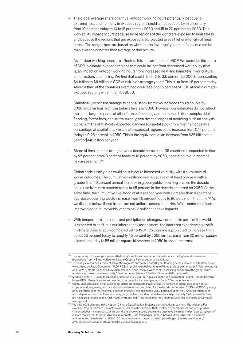
— The global average share of annual outdoor working hours potentially lost due to extreme heat and humidity in exposed regions could almost double by mid-century, from 10 percent today to 10 to 15 percent by 2030 and 15 to 20 percent by 2050. This workability impact occurs because more regions of the world are exposed to heat stress and because the regions that are exposed are projected to see higher intensity of heat stress. The ranges here are based on whether the “average” year manifests, or a colder than average or hotter than average period occurs.
— As outdoor working hours are affected, this has an impact on GDP. We consider the share of GDP in climate-exposed regions that could be lost from decreased workability (that is, an impact on outdoor working hours from increased heat and humidity) in agriculture, construction, and mining. We find that could rise to 2 to 3.5 percent by 2050, representing $4 trillion to $6 trillion in GDP at risk in an average year.158 This is up from 1.5 percent today. About a third of the countries examined could see 5 to 15 percent of GDP at risk in climate-exposed regions within them by 2050.
— Statistically expected damage to capital stock from riverine floods could double by 2030 and rise fourfold from today’s levels by 2050; however, our estimates do not reflect the much larger impacts of other forms of flooding or other hazards (for example, tidal flooding, forest fires, and storm surge) given the challenges of modeling such an analysis globally.159 The statistically expected damage to capital stock from riverine floods as a percentage of capital stock in climate-exposed regions could increase from 0.15 percent today to 0.25 percent in 2050. This is the equivalent of an increase from $35 billion per year to $140 billion per year.
— Share of time spent in drought over a decade across the 105 countries is expected to rise by 25 percent, from 8 percent today to 10 percent by 2050, according to our inherent risk assessment.160
— Global agriculture yields could be subject to increased volatility, with a skew toward worse outcomes. The cumulative likelihood over a decade of at least one year with a greater than 10 percent annual increase in global yields occurring once in the decade could rise from zero percent today to 45 percent in the decade centered on 2050. At the same time, the cumulative likelihood of at least one year with a greater than 10 percent decrease occurring would increase from 45 percent today to 90 percent in that time.161 As we discuss below, these trends are not uniform across countries. While some could see improved agricultural yields, others could suffer negative impacts.
— With temperature increases and precipitation changes, the biome in parts of the world is expected to shift.162 In our inherent risk assessment, the land area experiencing a shift in climate classification compared with a 1901–25 baseline is projected to increase from about 25 percent today to roughly 45 percent by 2050 (an increase from 30 million square kilometers today to 55 million square kilometers in 2050 in absolute terms).
158 The lower end of the range assumes that today’s sectoral composition persists, while the higher end is based on projections from IHS Markit Economics and Country Risk on sectoral transitions.
159 This analysis assumes sufficient adaptation against current 50- to 100-year flooding events. Choice of adaptation levels were based on Paolo Scussolini, “FLOPROS: an evolving global database of flood protection standards,” Natural Hazards and Earth Systems Sciences, May 2016, Volume 16 and Philip J. Ward et al., “Assessing flood risk at the global scale: model setup, results, and sensitivity,” Environmental Research Letters, October 2013, Volume 8.
160 Modeled by WHRC using the median projection of 20 CMIP5 GCMs, using the self-correcting Palmer Drought Severity Index (PDSI). Projections were corrected to account for increasing atmospheric CO2 concentrations.
161 Global yields based on an analysis of six global breadbaskets that make up 70 percent of global production of four crops: wheat, soy, maize, and rice. Cumulative likelihood calculated for the decade centered on 2030 and 2050 by using annual probabilities for the climate state in the 2030 period and the 2050 period, respectively. Annual probabilities are independent and can therefore be aggregated to arrive at a cumulative decadal probability. Yield anomalies here are measured relative to the 1998–2017 average yield. Yield anomalies here are measured relative to the 1998—2017 average yield.
162 We have used changes in the Köppen Climate Classification System as an indicative proxy for shifts in biome. For example, tropical rainforests exist in a particular climatic envelope that is defined by temperature and precipitation characteristics. In many parts of the world, this envelope could begin to be displaced by a much drier “tropical savannah” climate regime that threatens tropical rainforests. Data taken from Franz Rubel and Markus Kottek, “Observed and projected climate shifts 1901–2100 depicted by world maps of the Köppen-Geiger climate classification,” Meteorologische Zeitschrift, April 2010, Volume 19, Number 2.
94 McKinsey Global Institute

Box 4Why we have not made an estimate of the impact of climate change and adaptation on global GDP
1 W. J. Wouter Botzen, Olivier Deschenes, and Mark Sanders, “The economic impacts of natural disasters: A review of models and empirical studies,” Review of Environmental Economics and Policy, Summer 2019, Volume 13, Number 2.
2 Roberto Roson and Dominique van der Mensbrugghe, “Climate change and economic growth: impacts and interactions,” International Journal of Sustainable Economy, 2012, Volume 4, Issue 3; Frank Ackerman et al., “Fat tails, exponents, extreme uncertainty: Simulating catastrophe in DICE,” Ecological Economics, 2010, Volume 69, Issue 8; Tom Kompas et al., “The Effects of Climate Change on GDP by Country and the Global Economic Gains From Complying With the Paris Climate Accord,” Earth’s Future, July 2018, Volume 6, Issue 8; Nicholas Stern, The economics of climate change: the Stern review. Cambridge, UK: Cambridge University Press, 2007.
3 Simon Dietz and Nicholas Stern, Endogenous growth, convexity of damages and climate risk: How Nordhaus’ framework supports deep cuts in carbon emissions, Grantham Research Institute on Climate Change and the Environment, June 2014; J. Doyne Farmer et al., “A third wave in the economics of climate change,” Environmental and Resource Economics, 2015, Volume 62, Number 2.
4 Marshall Burke, Solomon M. Hsiang, and Edward Miguel, “Global non-linear effect of temperature on economic production,” Nature, November 2015, Volume 527, Number 7577.
5 Matthew E. Kahn et al., Long-term macroeconomic effects of climate change: A cross-country analysis, Federal Reserve Bank of Dallas, Globalization Institute Working Paper 365, July 2019; Riccardo Colacito et al., The impact of higher temperatures on economic growth, The Federal Reserve Bank of Richmond, North Carolina, Economic Brief EB18-08, August 2018.
6 Steven C. Sherwood and Matthew Huber, “An adaptability limit to climate change due to heat stress.” Proceedings of the National Academy of Sciences, May 25, 2010, Volume 107, Number 21.
7 Simon Dietz and Nicholas Stern, Endogenous growth, convexity of damages and climate risk: How Nordhaus’ framework supports deep cuts in carbon emissions, Grantham Research Institute on Climate Change and the Environment, June 2014; Howard Covington and Raj Thamotheram, “The case for forceful stewardship (Part 1): The financial risk from global warming,” SSRN, January 19, 2015; Martin L. Weitzman, “GHG targets as insurance against catastrophic climate damages,” Journal of Public Economic Theory, March 2012, Volume 14, Number 2.
Estimating the full consequences of climate change for the global economic system is extremely challenging. As discussed earlier, there are many uncertainties, in particular with quantifying the second-order implications of the direct physical damages from a changing climate. Conceptually, economists treat climate as they do other assets, in terms of economic value. A depreciation of the value of this asset entails substantial consequences for the economic activity and well-being of the current as well as future generations.
Researchers have taken a variety of approaches in their attempts to quantify the GDP impacts of climate change and, in a related field, quantify the economic impact of natural disasters. These have broadly fallen into various forms of “macro” assessments or “micro” assessments.1
The most prominent macro approach includes integrated assessment models or IAMs that seek to integrate climate models with economic modeling by using “damage functions” relating temperature to impacts on capital stock. IAMs can produce estimates of a total value-at-risk of between 3-10 percent of GDP by the end of the century, under a business-as-usual scenario.2 Such models have been
critiqued for three reasons. Firstly, and most importantly, the damage functions used to estimate impact are generally arbitrarily chosen functions fit to limited empirical evidence. Secondly, they tend to explicitly assume that damages only impact output and do not interact with endogenous drivers of growth like investment. Thirdly, they largely do not simulate financial systems nor other important sources of second-order impact or risk contagion, including migration, loss of life, and conflict.3
A second macro approach has involved using econometric assessments of historical climate hazard data (typically temperature and precipitation), and then applying that assessment to explore future outcomes. Burke, Hsiang, and Miguel (2015) used econometric approaches to demonstrate that overall economic activity is a nonlinear function of temperature for all countries, with productivity peaking and then declining strongly at higher temperatures. This trend was found to be globally generalizable, unchanged since 1960, and apparent for agricultural and non-agricultural activity in both rich and poor countries. Based on these findings, the authors project that 10 to 60 percent of global GDP could be at risk by the end of the century under an RCP 8.5 scenario.4 An alternate
econometric approach by Kahn et al. (2019) finds a value more in line with IAM estimates, at roughly 7 percent of global GDP at risk by end-of-century, and a third approach by Colacito et al. (2018) estimates up to 33 percent of GDP at risk for the United States by end-of-century.5 The main source of difference across these approaches stems from their assumptions about how economic activity responds to temperature.
A third macro approach ties IAM damage functions at low levels of warming together with the physical science of high-warming outcomes, assuming GDP damages tending toward 100 percent above certain thresholds of warming. For example, at a 10- to 12-degree Celsius increase in global average temperatures, most of the world’s surface would have persistent summer temperatures above the habitability threshold for a healthy human being.6 Using this approach, Weitzman (2012), Dietz and Stern (2014), and Covington and Thamotheram (2015) find economic damages ranging between 10 and 50 percent of global GDP by end-of-century under an RCP 8.5 scenario.7
95Climate risk and response: Physical hazards and socioeconomic impacts
The wide ranges in the magnitude of GDP at risk established by these approaches reflect the high degree of uncertainty involved, primarily related to how economic systems will respond to changing climate hazards. To some degree, they also reflect assumptions related to an adaptation response and the evolution of climate hazards by the turn of the century. Many advances at the micro level have been made to address this uncertainty and better understand how specific aspects of climate change affect components of the economic system. The aim is to improve economic modeling from an understanding of the mechanisms by which climate change affects socioeconomic systems.8
Our research seeks to take such a step. Our case studies aim to shed light on the mechanisms by which a changing climate can affect socioeconomic systems. Translating those mechanisms to a global GDP-at-risk number is extremely challenging for all the reasons described above. We have therefore focused here on highlighting the nature of GDP implications as well as the magnitude of short-run GDP at risk for a subset of hazards.
While our case studies describe in more detail how GDP is affected by climate change for each individual hazard, region, and sector studied, some findings across our cases are worth noting. First, we find that the direct impacts of climate change are on the stocks of human, physical, and natural capital. Together, such stocks represent
8 The economic risks of climate change in the United States, Risky Business, 2019; The price of climate change: Global warming’s impact on portfolios, BlackRock, October 2015.
9 Jeroen Klomp and Kay Valckx, “Natural disasters and economic growth: A meta-analysis,” Global Environmental Change, May 2014, Volume 26, Number 1.10 Mark Skidmore and Hideki Toya, “Do natural disasters promote long-run growth ?” Economic Inquiry, October 2002, Volume 40, Number 4. 11 Daniel Cooper and Karen Dynan, “Wealth effects and macroeconomic dynamics,” Journal of Economic Surveys, February 2016, Volume 30, Number 1. 12 See Gilbert E. Metcalf and James H. Stock, “Integrated Assessment Models and the Social Cost of Carbon: A Review and Assessment of U.S. Experience,” Review of
Environmental Economics and Policy, Volume 11, 2017.13 Christian Gollier and James K. Hammitt, “The Long-Run Discount Rate Controversy,” Annual. Review of Resource Economics, April 2014, Volume 6; Thomas
Sterner and Efthymia Kyriakopoulou, “(The Economics of) Discounting: Unbalanced Growth, Uncertainty, and Spatial Considerations,” Annual. Review of Resource Economics, Volume 4, 2012.
14 See for example, Mark C. Freeman and Ben Groom, “How certain are we about the certainty-equivalent long term social discount rate?” Journal of Environmental Economics and Management, Volume 79, September 2016; Moritz A. Drupp et al., “Discounting discounted,” American Economic Journal: Economic Policy, Volume 10 Number 4, November 2018.
the productive capacity of economies. The impairment of these stocks could in turn have substantial effects on GDP (the economic flows that derive from stocks of capital). The compounding effect of diminished productive capacity over multiple years could potentially be significant. However, more research is needed to estimate how large the long-term effects could be.9 For example, in the short term, having to rebuild and replace damaged stock could stimulate GDP. In the long term, however, this may act as a drag on GDP growth, if it diverted funds from other investment opportunities (for example, replacing existing damaged structures rather than investing to expand productive capacity or develop new technologies). Alternately, if new investments are made with a focus on adaptation, resilience, and integrating new technologies into new capital stock, this could help boost GDP growth.10
Second, we find that impacts to GDP could occur through both supply- and demand-side effects. On the supply side, we find that a changing climate could have direct impacts on labor and capital productivity, and it could also destroy capital stock, diminishing capital services derived from such stock. There could also be knock-on effects on demand. For example, home owners might reduce consumption if their wealth were affected by a fall in real estate prices due to expectations of climate change.11 Falling property prices could also reduce government
tax revenue, with repercussions on government spending.
Third, our cases and global geospatial analysis demonstrate the spatial nature of climate risk. This means that the GDP at risk in specific regions may be significantly higher than in other regions, and significantly higher than a global average. On the flip side, some regions may see much lower-than-average risk, and in some respects like agricultural yields, may even stand to benefit.
As economists have evaluated the economic consequences of climate change, the costs of mitigating and adaptation measures are compared to the benefits arising from the expected reduction in damages result from climate-change. This comes with a number of issues. Firstly of course is assessing the damage functions and costs arising from climate change, as discussed above.12 Secondly, costs and benefits are defined relative to the preferences of individuals, which might be highly diverse, and which need to be evaluated over time. A key parameter in this debate is the discount rate to be applied to assess the overall implications of a changing climate over time and the level of burden sharing to be achieved between today’s consumers and producers and future generations.13 Identifying an appropriate discount rate is another much debated topic in the climate debate, but out of scope for this report.14
96 McKinsey Global Institute

Livability and workability As discussed in the India case, parts of South Asia are projected to become some of the first places over the coming decades to experience heat waves that surpass the survivability threshold for a healthy human being over the coming decades.163 We find a similar trend in other regions. Under an RCP 8.5 scenario, we find that by 2030, the number of people living in regions with a greater than zero percent annual probability of a lethal heat wave is projected to increase from negligible today to between about 250 million and 360 million, without factoring in air conditioner penetration. Today, air conditioner penetration is roughly 10 percent across India, and roughly 60 percent across China.164 This dramatic increase in exposed regions, and thus population, is due to the sharp right-hand tail of the distribution of wet-bulb temperatures. It takes a significant rightward (that is, higher) shift of the distribution of wet-bulb temperatures before lethal heat waves are possible, but once they become possible, the annual probability increases rapidly. The most heavily populated areas of the world are usually also among the hottest and most humid, and these areas are becoming even hotter and more humid.
For the 2030 period under an RCP 8.5 scenario, the average annual probability of a lethal heat wave occurring is estimated to be roughly 9 percent across exposed regions (that is, regions with a non-zero annual likelihood of such heat waves). Because this is an average number across regions, some regions have higher probabilities and others have lower.165 The average probability of a person living in an at-risk region experiencing such a lethal heat wave occurring once in the decade centered on 2030 is estimate to be approximately 60 percent.166 By 2050, the number of people living in regions experiencing a non-zero likelihood of such heat waves is projected to increase to between 700 million and 1.2 billion people, again without factoring in air conditioner penetration. People living in such regions are projected to have an average 14 percent annual probability of experiencing a lethal heat wave or a roughly 80 percent cumulative likelihood of experiencing such a heat wave at least once over a decade centered 2050.
As discussed in our India case, heat and humidity could also affect labor productivity, with workers needing to take more breaks and the human body naturally limiting its efforts to prevent over-exertion. We measure this effect by considering the effective working hours that could be at risk due to extreme heat and humidity in climate-exposed regions, a measure of impacts on workability.167 We consider an “average year,” predicted based on the mean of 20 climate models, as well as years that are “hotter and more humid than average” and “colder and less humid than average.”168 Considering the impact on workability, we find that today, about 10 percent of working hours are at risk globally due to conditions that reduce labor productivity in heat- and humidity-exposed regions. This is expected to rise to between 10 and 15 percent by 2030 and 15 to 20 percent by 2050, with the range reflecting the variation across years of different heat and humidity.
163 See the discussion of how we define lethal heat waves in Chapter 2. If a non-zero probability of lethal heat waves in certain regions occurred in the models for today, this was set to zero to account for the poor representation of the high levels of observed atmospheric aerosols in those regions in the CMIP5 models. High levels of atmospheric aerosols provide a cooling effect that masks the risk. See India case for further details. This analysis excludes grid-cells where the the likelihood of lethal heat waves is <1 percent, to eliminate areas of low statistical significance.
164 This estimate does not take into account current or future air-conditioning protection, and therefore should be viewed as an upper bound for exposure. India Cooling Action Plan Draft, Ministry of Environment, Forest & Climate Change, Government of India, September 2018; The Future of Cooling in China”, IEA, Paris, 2019.
165 We calculate the average annual probability in climate-exposed geographies by first calculating the number of people that live in any part of the world with a greater than zero probability of a lethal heat wave occurring. We then calculate, for each geospatial grid-cell with a non-zero probability of lethal heat wave occurrence, the product of the probability of the lethal heat wave occurring and the number of people in that grid-cell. The average annual probability of a lethal heat wave in climate-exposed geographies is then the division of those two numbers.
166 This calculation is a rough approximation. It assumes that the annual probability of X percent applies to every year in decade centered around 2030. We first calculate the cumulative probability of a heat wave not occurring in the 2030 decade, which is 1 minus X percent raised to the power 10. The cumulative probability of a heat wave occurring at least once in the decade is then 1 minus that number. A similar approach is followed for the 2050 cumulative likelihood.
167 This is the statistically expected number of hours that are lost in an average year. We consider the probability of different wet-bulb temperatures occurring, and the labor capacity lost at each temperature. See India case and technical appendix for details.
168 Such years are calculated by looking at the 25th and 75th percentile ensemble projection.
97Climate risk and response: Physical hazards and socioeconomic impacts
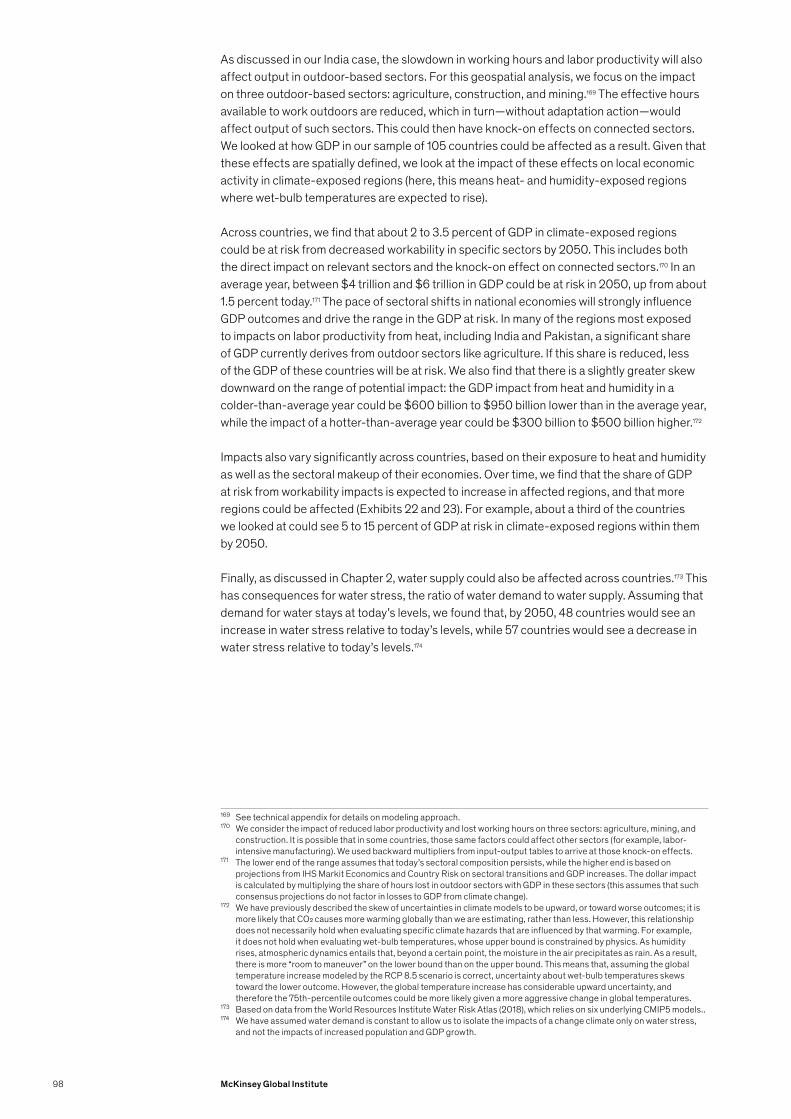
As discussed in our India case, the slowdown in working hours and labor productivity will also affect output in outdoor-based sectors. For this geospatial analysis, we focus on the impact on three outdoor-based sectors: agriculture, construction, and mining.169 The effective hours available to work outdoors are reduced, which in turn—without adaptation action—would affect output of such sectors. This could then have knock-on effects on connected sectors. We looked at how GDP in our sample of 105 countries could be affected as a result. Given that these effects are spatially defined, we look at the impact of these effects on local economic activity in climate-exposed regions (here, this means heat- and humidity-exposed regions where wet-bulb temperatures are expected to rise).
Across countries, we find that about 2 to 3.5 percent of GDP in climate-exposed regions could be at risk from decreased workability in specific sectors by 2050. This includes both the direct impact on relevant sectors and the knock-on effect on connected sectors.170 In an average year, between $4 trillion and $6 trillion in GDP could be at risk in 2050, up from about 1.5 percent today.171 The pace of sectoral shifts in national economies will strongly influence GDP outcomes and drive the range in the GDP at risk. In many of the regions most exposed to impacts on labor productivity from heat, including India and Pakistan, a significant share of GDP currently derives from outdoor sectors like agriculture. If this share is reduced, less of the GDP of these countries will be at risk. We also find that there is a slightly greater skew downward on the range of potential impact: the GDP impact from heat and humidity in a colder-than-average year could be $600 billion to $950 billion lower than in the average year, while the impact of a hotter-than-average year could be $300 billion to $500 billion higher.172
Impacts also vary significantly across countries, based on their exposure to heat and humidity as well as the sectoral makeup of their economies. Over time, we find that the share of GDP at risk from workability impacts is expected to increase in affected regions, and that more regions could be affected (Exhibits 22 and 23). For example, about a third of the countries we looked at could see 5 to 15 percent of GDP at risk in climate-exposed regions within them by 2050.
Finally, as discussed in Chapter 2, water supply could also be affected across countries.173 This has consequences for water stress, the ratio of water demand to water supply. Assuming that demand for water stays at today’s levels, we found that, by 2050, 48 countries would see an increase in water stress relative to today’s levels, while 57 countries would see a decrease in water stress relative to today’s levels.174
169 See technical appendix for details on modeling approach.170 We consider the impact of reduced labor productivity and lost working hours on three sectors: agriculture, mining, and
construction. It is possible that in some countries, those same factors could affect other sectors (for example, labor-intensive manufacturing). We used backward multipliers from input-output tables to arrive at those knock-on effects.
171 The lower end of the range assumes that today’s sectoral composition persists, while the higher end is based on projections from IHS Markit Economics and Country Risk on sectoral transitions and GDP increases. The dollar impact is calculated by multiplying the share of hours lost in outdoor sectors with GDP in these sectors (this assumes that such consensus projections do not factor in losses to GDP from climate change).
172 We have previously described the skew of uncertainties in climate models to be upward, or toward worse outcomes; it is more likely that CO2 causes more warming globally than we are estimating, rather than less. However, this relationship does not necessarily hold when evaluating specific climate hazards that are influenced by that warming. For example, it does not hold when evaluating wet-bulb temperatures, whose upper bound is constrained by physics. As humidity rises, atmospheric dynamics entails that, beyond a certain point, the moisture in the air precipitates as rain. As a result, there is more “room to maneuver” on the lower bound than on the upper bound. This means that, assuming the global temperature increase modeled by the RCP 8.5 scenario is correct, uncertainty about wet-bulb temperatures skews toward the lower outcome. However, the global temperature increase has considerable upward uncertainty, and therefore the 75th-percentile outcomes could be more likely given a more aggressive change in global temperatures.
173 Based on data from the World Resources Institute Water Risk Atlas (2018), which relies on six underlying CMIP5 models..174 We have assumed water demand is constant to allow us to isolate the impacts of a change climate only on water stress,
and not the impacts of increased population and GDP growth.
98 McKinsey Global Institute

Exhibit 22
GDP at risk from the effect of extreme heat and humidity on effective working hours is expected to increase over time.
Source: IHS Markit Economics and Country Risk; Woods Hole Research Center; McKinsey Global Institute analysis
Note: See the Technical Appendix for why we chose RCP 8.5. All projections based on RCP 8.5, CMIP 5 multi model ensemble. Heat data bias corrected. These maps do not consider sectoral shifts when projecting impact on labor productivity into the future—the percentage and spatial distribution of outdoor labor are held constant. For this analysis, outdoor labor is considered to include agriculture, construction, and mining and quarrying only, and knock-on impacts on other sectors are not considered. Following standard practice, we define current and future (2030, 2050) states as the average climatic behavior over multidecade periods. Climate state today is defined as average conditions between 1998 and 2017, in 2030 as average between 2021 and 2040, and in 2050 as average between 2041 and 2060.
GDP at risk from working hours impacted by heat and humidity (direct effect only, scenario of no sectoral transitions)%
≤0.1
0.2–1.0
1.1–5.0
5.1–10.0
10.1–15.0
15.1–20.0
>20
Today
2030
2050
Based on RCP 8.5
99Climate risk and response: Physical hazards and socioeconomic impacts
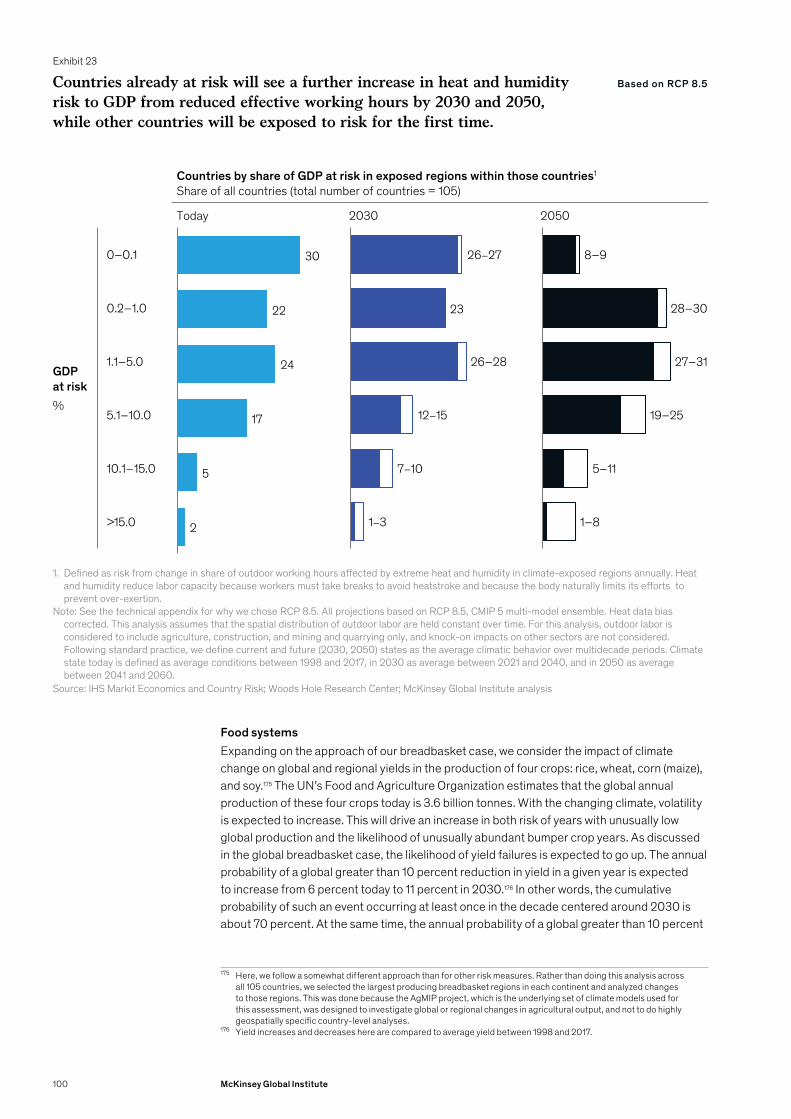
Food systemsExpanding on the approach of our breadbasket case, we consider the impact of climate change on global and regional yields in the production of four crops: rice, wheat, corn (maize), and soy.175 The UN’s Food and Agriculture Organization estimates that the global annual production of these four crops today is 3.6 billion tonnes. With the changing climate, volatility is expected to increase. This will drive an increase in both risk of years with unusually low global production and the likelihood of unusually abundant bumper crop years. As discussed in the global breadbasket case, the likelihood of yield failures is expected to go up. The annual probability of a global greater than 10 percent reduction in yield in a given year is expected to increase from 6 percent today to 11 percent in 2030.176 In other words, the cumulative probability of such an event occurring at least once in the decade centered around 2030 is about 70 percent. At the same time, the annual probability of a global greater than 10 percent
175 Here, we follow a somewhat different approach than for other risk measures. Rather than doing this analysis across all 105 countries, we selected the largest producing breadbasket regions in each continent and analyzed changes to those regions. This was done because the AgMIP project, which is the underlying set of climate models used for this assessment, was designed to investigate global or regional changes in agricultural output, and not to do highly geospatially specific country-level analyses.
176 Yield increases and decreases here are compared to average yield between 1998 and 2017.
Exhibit 23
Countries by share of GDP at risk in exposed regions within those countries1
Share of all countries (total number of countries = 105)
Today 2030 2050
GDP at risk%
0–0.1
0.2–1.0
1.1–5.0
5.1–10.0
10.1–15.0
>15.0
Countries already at risk will see a further increase in heat and humidity risk to GDP from reduced effective working hours by 2030 and 2050, while other countries will be exposed to risk for the first time.
Source: IHS Markit Economics and Country Risk; Woods Hole Research Center; McKinsey Global Institute analysis
1. Defined as risk from change in share of outdoor working hours affected by extreme heat and humidity in climate-exposed regions annually. Heat and humidity reduce labor capacity because workers must take breaks to avoid heatstroke and because the body naturally limits its efforts to prevent over-exertion.
Note: See the technical appendix for why we chose RCP 8.5. All projections based on RCP 8.5, CMIP 5 multi-model ensemble. Heat data bias corrected. This analysis assumes that the spatial distribution of outdoor labor are held constant over time. For this analysis, outdoor labor is considered to include agriculture, construction, and mining and quarrying only, and knock-on impacts on other sectors are not considered. Following standard practice, we define current and future (2030, 2050) states as the average climatic behavior over multidecade periods. Climate state today is defined as average conditions between 1998 and 2017, in 2030 as average between 2021 and 2040, and in 2050 as average between 2041 and 2060.
30
22
24
17
5
2
23
1–3
26–27
12–15
26–28
7–10
8–9
28–30
19–25
27–31
5–11
1–8
Based on RCP 8.5
100 McKinsey Global Institute

increase in yield in a given year is not expected to change meaningfully between now and 2030. By 2050, the annual probability of a greater than 10 percent reduction in yield in a given year is expected to further increase to about 20 percent (or, is expected to occur a 90 percent cumulative probability once in the decade centered around 2050) while the probability of a greater than 10 percent increase in yield in a given year is expected to increase to 6 percent (or, has about a 45 percent chance of occurring once in the decade centered around 2050).
Thus, our analysis suggests variability in both good and bad outcomes, although the volatility is likely to be skewed toward worse outcomes. These shifts in agricultural output will affect agricultural GDP. The tail GDP risk would increase over time as the likelihood of a global reduction in production increases; moreover, the impact of diminished agricultural production could also have knock-on effects through the economy, affecting food prices, consumption, and downstream industries, as discussed in the breadbasket case.
Global findings also hide heterogenous regional trends: some regions are projected to experience increases in statistically expected yields, while others are projected to experience decreases. All regions are projected to experience an increase in volatility, but in some regions that volatility would be skewed toward better outcomes, while in other regions the skew would be toward worse outcomes. While we were not able to exhaustively investigate all regions, we were able to identify some differing regional trends in the large producing parts of the world. For example:
— North America. The United States on average is expected to experience net-negative consequences, with statistically expected yields decreasing and volatility skewed toward worse outcomes. By contrast, Canada is expected to see sharp increases in statistically expected yields. The United States is expected to see a greater than 10 percent decrease in statistically expected yields by 2050 compared with the 1998–2017 period, with the annual probability of a greater than 10 percent decrease in yield in a given year increasing from 20 percent today to 50 percent by 2050. The annual probability of a bumper year with a greater than 10 percent increase in yields relative to the 1998–2017 baseline is expected to increase from 0 percent to 6 percent. Canada is expected to see a 50 percent increase in statistically expected yields by 2050 relative to 1998–2017. The annual probability of a greater than 10 percent decrease in yields in a given year is expected to decrease from 16 percent today to 0 percent by 2050, and the annual probability of a greater than 10 percent bumper crop year is expected to increase from 17 percent today to 98 percent by 2050.
— South America. South America is a climatologically diverse continent that experiences different agricultural outcomes in different regions. The largest single producer in the region is Brazil. Like the United States, Brazil is expected to suffer net-negative agricultural consequences from climate change, with both decreasing statistically expected yields and volatility skewed toward worse outcomes. Specifically, Brazil is expected to see a 3 percent decrease in statistically expected annual yields by 2050 relative to 1998–2017. The annual probability of a greater than 10 percent yield decline in a given year compared with a 1998–2017 baseline would increase from 3 percent today to 10 percent by 2050, whereas the probability of a 10 percent yield increase is not expected to change meaningfully.
— Europe. Europe and western Russia could together experience net agricultural benefits as a result of climate change, with increasing statistically expected yields, and an increase in volatility skewed toward more positive outcomes. However, risk of yield failures does increase through to 2050, and there are many differences within the region. The aggregate region of Europe and Russia is expected to experience a 4 percent increase in statistically expected yields by 2050 relative to 1998–2017. The annual probability of a greater than 10 percent yield failure compared with a 1998–2017 baseline would increase from 8 percent to 11 percent by 2050, while the annual probability of a bumper year with a greater than 10 percent yield increase would rise from 8 percent to 18 percent by 2050.
101Climate risk and response: Physical hazards and socioeconomic impacts

— Asia–Pacific. China is expected to be an agricultural net beneficiary from climate change over the near term, with increasing statistically expected yields and volatility skewed toward positive outcomes. India, on the other hand, is expected to experience a net-negative agricultural impact from climate change. China could see expected yields increase by about 2 percent by 2050 relative to 1998–2017. The annual probability of greater than 10 percent breadbasket failure relative to a 1998–2017 baseline would decrease from 5 percent to 2 percent by 2050, while the annual probability of a bumper year with a greater than 10 percent increase in yield would increase from 1 percent to approximately 12 percent by 2050. India is expected to experience a 7 percent decrease in statistically expected crop yields by 2050, while the annual probability of a greater than 10 percent decrease in yields in a given year would increase from 10 percent to 40 percent by 2050. The annual probability of greater than 10 percent increase in yields in a given year would decrease from 3 percent to 0 percent over the same period.
Physical assets and infrastructure servicesAs we found in our cases, assets can be destroyed or service from infrastructure assets disrupted by a variety of hazards including flooding, forest fires, hurricanes, and heat. Take flooding, for example. There are various forms of flooding, including riverine floods, flash floods, storm surge, and tidal flooding, all of which could damage capital stock. Due to data limitations, we were unable to examine the impacts of each of these on capital stock globally, but we specifically look at the impact of one hazard—riverine flooding—to illustrate how global capital stock could be affected by rising climate hazards.177 The approach we take in our cases assesses the evolution of hazard severity and frequency and then overlays that with data on capital stock exposure and capital stock resilience.
Estimating capital stock damage from flooding is highly complex, and the numbers we give here should be taken as directional in their assessment of risk rather than as precise estimates.178 Moreover, it is important to recognize that such estimates are underestimates of the capital stock at risk of damage from a changing climate, since this represents only one specific hazard. Nonetheless, some important trends emerge. First, the growth in statistically expected damage to capital from riverine flooding is expected to rise steeply, from about $35 billion of capital stock every year globally today to about $60 billion by 2030 and $140 billion by 2050.179 This represents a 1.7-fold increase between today and 2030, and a fourfold increase between today and 2050. Impacts could be significantly higher than these numbers suggest, depending on the specific form of capital affected, such as infrastructure. This leads to various knock-on effects, as discussed in our infrastructure case.
The numbers above represent statistical averages, and the impacts could be significantly higher in a given year if tail events manifest. This is similar to our finding in the Florida case, where our analysis shows that statistical average impacts on real estate from storm surge could increase from $2 billion to between $3 billion and $4.5 billion between today and 2050, but the impact of 1-in-100-year storm surge events is substantially higher and could increase from $35 billion today to between $50 billion and $75 billion by 2050, an increase of 40 to 110 percent.
177 We chose to analyze riverine flooding due to ease of global data availability. 178 This analysis is based on using riverine floodplain data from the World Resources Institute to identify today’s floodplains
and data on increases in precipitation frequency to evaluate how flooding hazards could evolve. This approach therefore should be considered to be only an approximation of the evolution of flooding hazard, and it should be noted that a robust analysis of flooding will require the use of granular flood models. Further limitations of this analysis include the focus on riverine flooding only (versus tidal, flash, or pluvial flooding, or flooding from storm surge), the ability to identify flood protections globally in a robust way and therefore adjust for today’s level of adaptation, and the ability to identify damage functions for capital stock that are specific to an individual site, such as a given building or a factory, rather than rely on more general damage functions. See the technical appendix for modeling approach details.
179 This was calculated by using geospatial data on capital stock from UN Global Assessment Report on Disaster Risk Reduction, assessing exposure of the capital stock to flood depths of different severity, and using regional vulnerability assessments from the European Commission Joint Research Center. We assume that capital stock today is adapted to withstand today’s 50- and 100-year floods. We also assume capital stock increases going forward in line with today’s ratio of GDP and capital stock and based on consensus GDP projections from IHS Markit Economics and Country Risk. However, we assume that the geospatial breakdown of capital stock remains as today, given data limitations on obtaining time series estimates on how the geospatial breakdown of capital stock varies.
102 McKinsey Global Institute

Other researchers have attempted similar estimates for hurricane damage and its potential tail risks. For example, an analysis by the Cambridge Risk Studies Centre found that damage caused by a tail risk hurricane in the eastern United States could potentially be more than $1 trillion, because storms travel long distances and can make multiple landfalls. The Cambridge Risk Studies Centre classifies such a tail hurricane event as a 1-in-200-year event. This could begin as a normal tropical system of low-pressure clouds and thunderstorms, rapidly intensify upon entering the Gulf Stream, grow to a Category 4 hurricane in under six hours, then make landfall in Florida with sustained winds of over 147 miles per hour. It could move across the Gulf of Mexico and finally make second landfall near Santa Rosa Island, near Pensacola, but with lower sustained winds of 127 miles per hour and at Category 3 intensity. The Cambridge Risk Studies researchers expect recovery from the hurricane event would take around a year and personal consumption would dip to 83 percent in the first quarter after the disaster.180 Climate change contributes to the frequency of such hurricanes, the Cambridge Risk Studies Centre finds.
Natural capitalWith temperature increases and precipitation changes, the biome in many parts of the world is expected to shift. The biome refers to the naturally occurring community of flora and fauna inhabiting a particular region. For this report, we have used changes in the Köppen Climate Classification System as an indicative proxy for shifts in biome.181 For example, tropical rainforests exist in a particular climatic envelope that is defined by temperature and precipitation characteristics. In many parts of the world this envelope could begin to be displaced by a much drier “tropical savannah” climate regime, putting tropical rainforests at risk of collapse. Today, 25 percent of the Earth’s land area has already experienced a shift in climate classification compared with the 1901–25 period. By 2050, that number is expected to increase to roughly 45 percent. All countries and their local species would be affected to some degree, and in countries that rely on the natural environment, this could in particular affect ecosystem services and local livelihoods.
By 2030, every country could see an increase in one of our six indicators of potential impacts from a changing climate, with emerging economies facing the biggest increase Taking together a country view of the six indicators of potential climate impacts we examine—the share of population living in areas experiencing a non-zero annual probability of lethal heat waves, the share of outdoor working hours affected by extreme heat and humidity, the annual demand of water as a share of annual supply of water, the share of time spent in drought over a decade, the annual share of capital stock at risk of riverine flood damage in climate-exposed regions, and the share of land surface changing climate classification—we find that all 105 countries we studied would see an increase in the potential direct impacts from climate change as indicated by at least one measure by 2030. This could then increase further to 2050, under an RCP 8.5 scenario and without adaptation. As noted earlier in the chapter, 16 countries could see an increase in three indicators by 2050 compared to today, while 44 countries see an increase in five of six indicators. Most countries are expected to see rising impacts for the annual share of effective outdoor working hours affected by extreme heat and humidity in climate-exposed regions, annual share of capital stock at risk of flood damage in climate-exposed regions, and the share of land surface changing climate classification.
180 Impacts of severe natural catastrophes on financial markets, Cambridge Centre for Risk Studies, 2018. 181 Biome shift was measured using the Köppen climate classification system. The Köppen climate system divides climates
into five main groups, with each group further subdivided based on seasonal precipitation and temperature patterns. This is not a perfect system for assessing the location and composition of biomes; however, these two characteristics do correlate very closely with climate classification, and therefore this was assessed as a reasonable proxy for risk of disruptive biome changes.
103Climate risk and response: Physical hazards and socioeconomic impacts
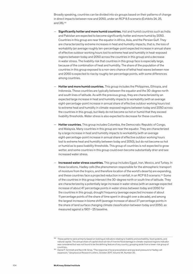
Broadly speaking, countries can be divided into six groups based on their patterns of change in direct impacts between now and 2050, under an RCP 8.5 scenario (Exhibits 24, 25, and 26).182
— Significantly hotter and more humid countries. Hot and humid countries such as India and Pakistan are expected to become significantly hotter and more humid by 2050. Countries in this group are near the equator in Africa, Asia, and the Persian Gulf. They are characterized by extreme increases in heat and humidity impacts, that is, the loss of workability (an average roughly ten-percentage-point expected increase in annual share of effective outdoor working hours lost to extreme heat and humidity in heat-exposed regions between today and 2050 across the countries in this group) and a decrease in water stress. The livability risk that countries in this group face is especially large, because of the combination of heat and humidity. The share of the population of the countries in this group exposed to a non-zero chance of lethal heat waves between now and 2050 is expected to rise by roughly ten percentage points, with some differences among countries.
— Hotter and more humid countries. This group includes the Philippines, Ethiopia, and Indonesia. These countries are typically between the equator and the 30-degree north and south lines of latitude. As with the previous group, they are characterized by an expected large increase in heat and humidity impacts to workability (with an average eight-percentage-point increase in annual share of effective outdoor working hours lost to extreme heat and humidity in climate-exposed regions between today and 2050 across the countries in this group), but likely do not become so hot or humid that they exceed livability thresholds. Water stress is also expected to decrease for these countries.
— Hotter countries. This group includes Colombia, the Democratic Republic of Congo, and Malaysia. Many countries in this group are near the equator. They are characterized by a large increase in heat and humidity impacts to workability (with an average eight-percentage-point increase in annual share of effective outdoor working hours lost to extreme heat and humidity between today and 2050), but do not become so hot or humid as to pass livability thresholds. This group of countries is not expected to grow wetter, and some countries in this group could even become substantially drier and see increased water stress.
— Increased water stress countries. This group includes Egypt, Iran, Mexico, and Turkey. In these locations, Hadley cells (the phenomenon responsible for the atmospheric transport of moisture from the tropics, and therefore location of the world’s deserts) are expanding, and these countries face a projected reduction in rainfall, in an RCP 8.5 scenario.183 Some of the countries in this group intersect the 30-degree north or south line of latitude. They are characterized by a potentially large increase in water stress (with an average expected increase of about 47 percentage points in water stress between today and 2050 for the countries in this group), drought frequency (average expected increase of about 11 percentage points of the share of time spent in drought over a decade), and among the largest increase in biome shift (average increase of about 27 percentage points in the share of land surface changing climate classification between today and 2050, as measured against a 1901—25 baseline.
182 These patterns were primarily based on looking at indicators relating to livability and workability, food systems, and natural capital. The annual share of capital stock at risk of riverine flood damage in climate-exposed regions indicator was considered but was not found to be the defining feature of any country, grouping aside from a lower-risk group of countries..
183 Daniel F. Schmidt and Kevin M. Grise, “The response of local precipitation and sea level pressure to Hadley cell expansion,” Geophysical Research Letters, October 2017, Volume 44, Number 20.
104 McKinsey Global Institute

— Lower-risk increase countries. This group includes Germany, Russia, and the United Kingdom. Many countries in this group lie outside the 30-degree north and south lines of latitude. They are generally cold countries and characterized by very low levels of heat and humidity impacts to workability (with an average 0.5-percentage-point increase in the annual share of effective outdoor working hours lost to extreme heat and humidity in climate-exposed regions, and no livability risk). Many are expected to see a decrease in overall impacts from indicators such as water stress or time spent in drought. As these countries grow warmer, one of the biggest changes they are likely to see is a significant shift in biome, for example as the polar and boreal climates retreat poleward and disappear. This group is expected to see the largest increase in biome change (about 40 percentage points average increase in the land surface changing climate classification between today and 2050, measured against a 1901—25 baseline. Another change that many of these countries could experience is an increase in the share of capital stock at risk of riverine flood damage in climate-exposed regions.
— Diverse climate countries. The final group consists of countries that span a large range of latitudes and therefore are climatically heterogeneous. Examples include Argentina, Brazil, Chile, China, and the United States.184 While average numbers may indicate small risk increases, these numbers mask wide regional variations. The United States, for example, has a hot and humid tropical climate in the Southeast, which could see significant increases in heat and humidity risk to outdoor work in our inherent risk scenario but is not projected to see increased water stress. The West Coast region, by contrast, is not expected to see a big increase in heat and humidity risk to outdoor work, but it is projected to have increased impacts from water stress and drought. In Alaska, the primary risk will likely be the shifting boreal biome affecting natural capital and the attendant ecosystem disruptions. To understand the climate risks facing diverse climate countries, one must examine the different regions independently.
184 To some extent, many countries could experience diversity of risk within their boundaries, a key feature of climate risk which is spatial. Here we have focused on highlighting countries with large climatic variations, and longitudinal expanse, which drives different outcomes in different parts of the country.
105Climate risk and response: Physical hazards and socioeconomic impacts
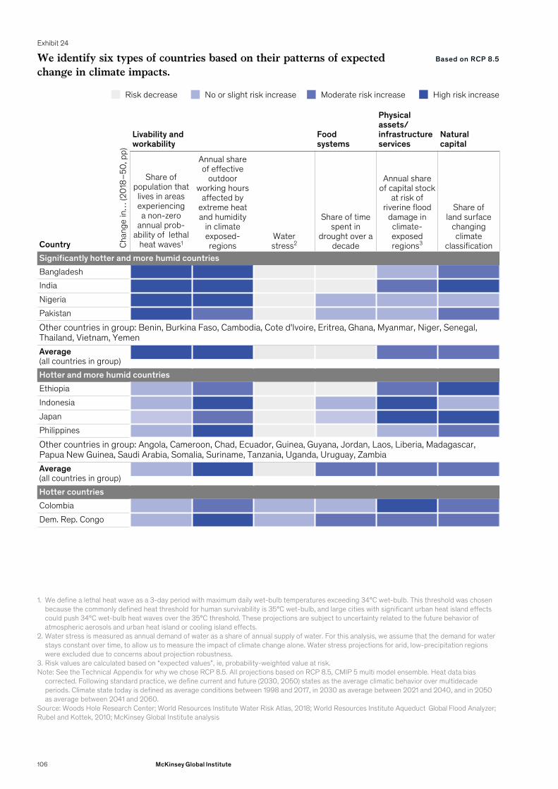
Exhibit 24
We identify six types of countries based on their patterns of expected change in climate impacts.
Source: Woods Hole Research Center; World Resources Institute Water Risk Atlas, 2018; World Resources Institute Aqueduct Global Flood Analyzer; Rubel and Kottek, 2010; McKinsey Global Institute analysis
1. We define a lethal heat wave as a 3-day period with maximum daily wet-bulb temperatures exceeding 34°C wet-bulb. This threshold was chosen because the commonly defined heat threshold for human survivability is 35°C wet-bulb, and large cities with significant urban heat island effects could push 34°C wet-bulb heat waves over the 35°C threshold. These projections are subject to uncertainty related to the future behavior of atmospheric aerosols and urban heat island or cooling island effects.
2. Water stress is measured as annual demand of water as a share of annual supply of water. For this analysis, we assume that the demand for water stays constant over time, to allow us to measure the impact of climate change alone. Water stress projections for arid, low-precipitation regions were excluded due to concerns about projection robustness.
3. Risk values are calculated based on “expected values”, ie, probability-weighted value at risk.Note: See the Technical Appendix for why we chose RCP 8.5. All projections based on RCP 8.5, CMIP 5 multi model ensemble. Heat data bias
corrected. Following standard practice, we define current and future (2030, 2050) states as the average climatic behavior over multidecade periods. Climate state today is defined as average conditions between 1998 and 2017, in 2030 as average between 2021 and 2040, and in 2050 as average between 2041 and 2060.
Based on RCP 8.5
Chan
ge in
… (2
018–
50, p
p)Livability and workability
Food systems
Physical assets/infrastructure services
Natural capital
Country
Share of population that
lives in areas experiencing a non-zero
annual prob-ability of lethal
heat waves1
Annual share of effective
outdoor working hours
affected by extreme heat and humidity
in climate exposed-regions
Waterstress2
Share of time spent in
drought over a decade
Annual share of capital stock
at risk of riverine flood
damage in climate-exposed regions3
Share of land surface
changing climate
classificationSignificantly hotter and more humid countriesBangladeshIndiaNigeriaPakistanOther countries in group: Benin, Burkina Faso, Cambodia, Cote d'Ivoire, Eritrea, Ghana, Myanmar, Niger, Senegal, Thailand, Vietnam, YemenAverage(all countries in group)Hotter and more humid countriesEthiopiaIndonesiaJapanPhilippinesOther countries in group: Angola, Cameroon, Chad, Ecuador, Guinea, Guyana, Jordan, Laos, Liberia, Madagascar, Papua New Guinea, Saudi Arabia, Somalia, Suriname, Tanzania, Uganda, Uruguay, ZambiaAverage(all countries in group)Hotter countriesColombiaDem. Rep. Congo
Risk decrease No or slight risk increase Moderate risk increase High risk increase
106 McKinsey Global Institute
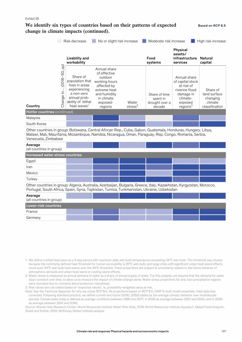
Exhibit 25
We identify six types of countries based on their patterns of expected change in climate impacts (continued).
Source: Woods Hole Research Center; World Resources Institute Water Risk Atlas, 2018; World Resources Institute Aqueduct Global Flood Analyzer; Rubel and Kottek, 2010; McKinsey Global Institute analysis
1. We define a lethal heat wave as a 3-day period with maximum daily wet-bulb temperatures exceeding 34°C wet-bulb. This threshold was chosen because the commonly defined heat threshold for human survivability is 35°C wet-bulb, and large cities with significant urban heat island effects could push 34°C wet-bulb heat waves over the 35°C threshold. These projections are subject to uncertainty related to the future behavior of atmospheric aerosols and urban heat island or cooling island effects.
2. Water stress is measured as annual demand of water as a share of annual supply of water. For this analysis, we assume that the demand for water stays constant over time, to allow us to measure the impact of climate change alone. Water stress projections for arid, low-precipitation regions were excluded due to concerns about projection robustness.
3. Risk values are calculated based on “expected values”, ie, probability-weighted value at risk.Note: See the Technical Appendix for why we chose RCP 8.5. All projections based on RCP 8.5, CMIP 5 multi model ensemble. Heat data bias
corrected. Following standard practice, we define current and future (2030, 2050) states as the average climatic behavior over multidecade periods. Climate state today is defined as average conditions between 1998 and 2017, in 2030 as average between 2021 and 2040, and in 2050 as average between 2041 and 2060.
Based on RCP 8.5
Chan
ge in
… (2
018–
50, p
p)Livability and workability
Food systems
Physical assets/infrastructure services
Natural capital
Country
Share of population that
lives in areas experiencing a non-zero
annual prob-ability of lethal
heat waves1
Annual share of effective
outdoor working hours
affected by extreme heat and humidity
in climate exposed-regions
Waterstress2
Share of time spent in
drought over a decade
Annual share of capital stock
at risk of riverine flood
damage in climate-exposed regions3
Share of land surface
changing climate
classificationHotter countries (continued)MalaysiaSouth KoreaOther countries in group: Botswana, Central African Rep., Cuba, Gabon, Guatemala, Honduras, Hungary, Libya, Malawi, Mali, Mauritania, Mozambique, Namibia, Nicaragua, Oman, Paraguay, Rep. Congo, Romania, Serbia, Venezuela, ZimbabweAverage(all countries in group)Increased water stress countriesEgyptIranMexicoTurkeyOther countries in group: Algeria, Australia, Azerbaijan, Bulgaria, Greece, Italy, Kazakhstan, Kyrgyzstan, Morocco, Portugal, South Africa, Spain, Syria, Tajikistan, Tunisia, Turkmenistan, Ukraine, UzbekistanAverage(all countries in group)Lower-risk countriesFranceGermany
Risk decrease No or slight risk increase Moderate risk increase High risk increase
107Climate risk and response: Physical hazards and socioeconomic impacts

Exhibit 26
We identify six types of countries based on their patterns of expected change in climate impacts (continued).
Source: Woods Hole Research Center; World Resources Institute Water Risk Atlas, 2018; World Resources Institute Aqueduct Global Flood Analyzer; Rubel and Kottek, 2010; McKinsey Global Institute analysis
1. We define a lethal heat wave as a 3-day period with maximum daily wet-bulb temperatures exceeding 34°C wet-bulb. This threshold was chosen because the commonly defined heat threshold for human survivability is 35°C wet-bulb, and large cities with significant urban heat island effects could push 34°C wet-bulb heat waves over the 35°C threshold. These projections are subject to uncertainty related to the future behavior of atmospheric aerosols and urban heat island or cooling island effects.
2. Water stress is measured as annual demand of water as a share of annual supply of water. For this analysis, we assume that the demand for water stays constant over time, to allow us to measure the impact of climate change alone. Water stress projections for arid, low-precipitation regions were excluded due to concerns about projection robustness.
3. Risk values are calculated based on “expected values”, ie, probability-weighted value at risk.4. Calculated assuming constant exposure. Constant exposure means that we do not factor in any increases in population or assets, or shifts in the
spatial mix of population and assets. This was done to allow us to isolate the impact of climate change alone. Color coding for each column based on the spread observed across countries within the indicator.
Note: See the Technical Appendix for why we chose RCP 8.5. All projections based on RCP 8.5, CMIP 5 multi model ensemble. Heat data bias corrected. Following standard practice, we define current and future (2030, 2050) states as the average climatic behavior over multidecade periods. Climate state today is defined as average conditions between 1998 and 2017, in 2030 as average between 2021 and 2040, and in 2050 as average between 2041 and 2060.
Based on RCP 8.5
Chan
ge in
… (2
018–
50, p
p)Livability and workability
Food systems
Physical assets/infrastructure services
Natural capital
Country
Share of population that
lives in areas experiencing a non-zero
annual prob-ability of lethal
heat waves1
Annual share of effective
outdoor working hours
affected by extreme heat and humidity
in climate exposed-regions
Waterstress2
Share of time spent in
drought over a decade
Annual share of capital stock
at risk of riverine flood
damage in climate-exposed regions3
Share of land surface
changing climate
classificationLower-risk countries (continued)RussiaUnited KingdomOther countries in group: Austria, Belarus, Canada, Finland, Iceland, Mongolia, New Zealand, Norway, Peru, Poland, SwedenAverage(all countries in group)Diverse climate countriesArgentinaBrazilChinaUnited StatesOther countries in group: ChileAverage(all countries in group)
Change in potential impact, 2018–504 (percentage points)Risk decrease n/a n/a <0 <0 <0 n/aSlight risk increase 0.0–0.5 0.0–0.5 0–3 0–3 0–0.05 0–5Moderate risk increase 0.5–5.0 0.5–5.0 3–7 3–7 0.05–0.10 5–10High risk increase >5.0 >5.0 >7 >7 >0.10 >10
Risk decrease No or slight risk increase Moderate risk increase High risk increase
108 McKinsey Global Institute

Countries and regions with lower per capita GDP levels are generally more at risk. Poorer regions often have climates that are closer to physical thresholds. They rely more on outdoor work and natural capital and have fewer financial means to adapt quickly, meaning that they could be more vulnerable to the effects of climate change.185 Climate change could also benefit some countries; for example, crop yields in Canada, Russia, and parts of Northern Europe could improve.
The risk associated with the impact on workability from rising heat and humidity is one example of how poorer countries are more exposed to hazards (Exhibit 27). When looking at the workability indicator (that is, the annual share of effective outdoor working hours lost to extreme heat and humidity), the top quartile of countries (based on GDP per capita) have an average increase in risk by 2050 of approximately one to three percentage points, whereas the bottom quartile faces an average increase in risk of approximately five to ten percentage points. Lethal heat waves show less of a correlation with per capita GDP, but it is important to note that several of the most affected countries, under an RCP 8.5 scenario, including Bangladesh, India, and Pakistan, have relatively low per capita GDP levels. Such countries are close to physical thresholds particularly for heat and humidity impacts on workability and livability.
Biome shift is expected to affect northern and southern latitude countries. Since many of these countries have higher per capita GDP levels, this indicator shows a positive correlation with development levels.
185 Note that this could also be true at a sub-national level; specific regions and communities could be more vulnerable than others within a country.
109Climate risk and response: Physical hazards and socioeconomic impacts
Exhibit 27
Countries with the lowest per capita GDP levels face the biggest increase in risk for some indicators.
Source: Woods Hole Research Center; Rubel and Kottek, 2010; IMF; World Bank; UN; McKinsey Global Institute analysis
Change, 2018–50Percentage points
Annual share of effective outdoor working hours affected by extreme heat and humidity in climate-exposed regionsCorrelation coefficient:r = -0.49
Share of land surface changing climate classificationCorrelation coefficient:r = 0.35
1,000
4
100
14
2
10,0000
100,000
6
8
10
12
16
18
China
India
UnitedStates
Indonesia
Brazil
20
10,000
10
0100
40
1,000 100,000
30
60
50
70
80
90
100
GDP per capita, 2017 (current $)Log scale
ChinaUnitedStates
India
France
Arab statesAmericasAfrica Asia and the Pacific
Europe andCentral Asia
Note: Not to scale. See the Technical Appendix for why we chose RCP 8.5. All projections based on RCP 8.5, CMIP 5 multi model ensemble. Heat data bias corrected. Following standard practice, we define current and future (2030, 2050) states as the average climatic behavior over multidecade periods. Climate state today is defined as average conditions between 1998 and 2017, in 2030 as average between 2021 and 2040, and in 2050 as average between 2041 and 2060.
Based on RCP 8.5
110 McKinsey Global Institute

Our global geospatial analysis illustrates that current and future climate risk is pervasive across the world, with all 105 countries we studied experiencing an increase in at least one risk indicator by 2030. As we have highlighted in this report, sizing that risk is a complex task that requires an analysis of both statisticially expected and tail risks, of direct impacts to the stock of human, physical, and natural capital as well as to flows of GDP activity and other knock-on effects. Given these uncertainties and risks, how should decision makers respond? In the next chapter, we look at steps for stakeholders seeking an effective response to the challenges of a changing climate and the risks that it entails.
111Climate risk and response: Physical hazards and socioeconomic impacts

Sea gates offer a way to mediate the physical threat while wind turbines and other renewables offer a way forward. © Getty images
5. An effective response
Physical climate risk will affect everyone, directly or indirectly. Responding to it adequately will require careful translation of climate science into specific risk assessments, at a time when old models of assessing and managing risk are losing their relevance. As we have noted in this report, physical and socioeconomic impacts of climate change are characterized by the growing likelihood of long tail events occurring that could result in cascading systemic risks.
In this final chapter, we discuss three steps that stakeholders could consider as they seek an effective response to the socioeconomic impacts of physical climate risk: integrating climate risk into decision making, accelerating the pace and scale of adaptation, and decarbonizing at scale to prevent a further buildup of risk.
Integrating climate risk into decision makingMuch as thinking about information systems and cyber-risks has become integrated into corporate and public sector decision making, climate change will also need to feature as a major factor in decisions. As we have noted, physical climate risk is simultaneously spatial and systemic, non-stationary, and can result in nonlinear impacts. We find potential impacts to be rising over time across our cases and regressive; moreover, stakeholders today may be under-prepared to manage its impact. Decision making will need to reflect these characteristics. For companies, this will mean taking climate considerations into account when looking at capital allocation, development of products or services, and supply-chain management, among others. For example, large capital projects could be evaluated reflecting the full probability distribution of possible climate hazards at their location. This would include changes in that probability distribution over time and possible changes in cost of capital for exposed assets, as well as how climate risk could affect the broader market context and other implicit assumptions in the investment case. For cities, a climate focus will become essential for urban planning decisions. Moreover, while this report has focused on physical risk, a comprehensive risk management strategy will also need to include an assessment of transition and liability risk, and the interplay between these forms of risk.
Developing a robust quantitative understanding of climate risk is complex, for the many reasons outlined in this report. It requires the use of new tools, metrics, and analytics. Companies and communities are beginning to assess their exposure to climate risk, but much more needs to be done. Lack of understanding significantly increases risks and potential impacts across financial markets, and socioeconomic systems, for example, by driving capital flows to risky geographies, or increasing the likelihood of stakeholders being caught unprepared.
At the same time, opportunities from the changing climate will emerge and require consideration. These could arise from a change in the physical environment, such as new places for agricultural production, or for sectors like tourism, as well as through the use of new technologies and approaches to manage risk in a changing climate.
113Climate risk and response: Physical hazards and socioeconomic impacts
Changes in mind-set, operating model, and tools and processes will be needed to integrate climate risk into decision making effectively. Decision makers’ experiences are based on a world of relative climate stability, and they may not yet be planning for a world of changing climate. For example, statistical risk management is often not part of ordinary processes in industrial companies. With the changing climate, it will be important to understand and embrace the probabilistic nature of climate risk and be mindful of possible biases and outdated mental models; experiences and heuristics of the past are often no longer a reliable guide to the future. The systemic nature of climate risk requires a holistic approach to understand and identify the full range of possible direct and indirect impacts. The spatial nature of hazard means that decision making will need to incorporate a geographic dimension.
One of the biggest challenges from climate risk could be to rethink the current models we use to quantify risk. These range from financial models used to make capital allocation decisions, to engineering models used to design structures. As we have discussed, some uncertainty is associated with a methodology that leverages global and regional climate models, makes underlying assumptions on emissions paths, and seeks to translate climate hazards to potential physical and financial damages. The highest “model risk,” however, may not come from exploring new ways to quantify climate risk. Instead, it may derive from continued reliance on current models that are based on stable historical climate and economic data. These models have at least three potential flaws:
— The absence of geographic granularity. Most models do not take into account geospatial dimensions. As this report highlights, direct impacts of climate change are local in nature. This requires an understanding of the exposure to risk via geospatial analysis. For example, companies will need to understand how their global asset footprint is exposed to different forms of current and evolving climate hazard in each one of their main locations—and indeed in each of the main locations of their critical suppliers.
— The “non-stationarity,” or constant state of change, of the climate. For example, our entire capital stock is built around physical assumptions that may well be obsolete as relevant climate variables have already changed and continue to change. As a result, assumptions based on historical precedent and experience will need to be rethought. That could include, for example, how resilient to make new factories, what tolerance levels to employ in new infrastructure, and how to design urban areas.
— Potential sample bias could prove to be a flaw. Decision makers often rely on their own experiences as a frame for decision making; in a changing climate, this may result in an incorrect assessment of future risk.
A transformation in operating model could mean optimizing for resiliency rather than simply for efficiency. For example, it may be preferable to rent rather than own fixed assets. Companies may need to think about ways to increase resilience in supply chains, for example, by raising inventory levels or sourcing from multiple locations or suppliers. Resilience will need to be incorporated into capital design, and owners of well-functioning assets will need to maintain them proactively rather than waiting to repair damages.
Adequate tools, metrics, and processes will vary by stakeholder but will likely include transitioning from a reliance on historical data or “worst case” expectations based on experience to relying on climate modeling tools to prepare for the future, including building new analytics capabilities. The process of managing climate change incorporates a full risk diagnostic as the basis for an appropriate response strategy.
114 McKinsey Global Institute
Accelerating the pace and scale of adaptationSocieties have been adapting to the changing climate, but the pace and scale of adaptation will likely need to increase significantly. Key adaptation measures include protecting people and assets, building resilience, reducing exposure, and ensuring that appropriate insurance and financing are in place.
Implementing adaptation measures could be challenging for many reasons. With hazard intensity projected to increase, the economics of adaptation could worsen over time and there may eventually be technical or other limits to effective adaptation. In other instances, there could be difficult trade-offs that need to be assessed, including who and what to protect, and who and what to relocate.
In some instances, coordinated action across multiple stakeholders may be required. This may include establishing building codes and zoning regulations, mandating insurance or disclosures, mobilizing capital through risk-sharing mechanisms, sharing best practices across industry groups, and driving innovation. This could be done, for example, by providing tools to integrate climate risk into investment decisions, integrating diverse perspectives including those of different generations into decision making, and addressing the inequalities that climate risk could amplify.
Protecting people and assetsProtecting people is crucial. Steps can range from prioritizing emergency response and preparedness to erecting cooling shelters and adjusting working hours for outdoor workers exposed to heat. For example, the Ahmedabad City Corporation developed the first heat-action plan in India in response to the record-breaking 2010 heat wave that killed 300 people in a single day.186 As part of the plan, Ahmedabad has implemented programs to build the population’s awareness of the dangers of extreme heat. These measures include establishing a seven-day probabilistic heat-wave early-warning system, developing a citywide cool-roofs albedo management program, and setting up teams to distribute cool water and rehydration tablets to vulnerable populations during heat waves.187
Measures to harden existing infrastructure and assets to the extent possible can help limit risk. Hardening of infrastructure could include both “gray” infrastructure—for example, raising elevation levels of buildings in flood-prone areas—and natural capital or “green” infrastructure. One example of this is the Dutch Room for the River program, which gives rivers more room to manage higher water levels.188 Mangroves can also provide storm protection. A systemwide approach to protecting people and assets will be needed. For example, even as homes may need to be floodproofed, so too could the roadways near those homes.
Factoring decisions about protection into new buildings could be more cost-effective than retrofitting.189 For example, infrastructure systems or factories could be designed to withstand what used to be a one in 200-year event. With a changing climate, what constitute such an event may look different, and design parameters may need to be reassessed. Estimates suggest that $30 trillion to $50 trillion will be spent on infrastructure in the next ten years, much of it in developing countries.190 Given the lifetime of the assets, new infrastructure will
186 Kim Knowlton et al., “Development and implementation of South Asia’s first heat-health action plan in Ahmedabad (Gujarat, India),” International Journal of Environmental Research and Public Health, 2014, Volume 11, Issue 4.
187 Albedo refers to the reflectivity of a surface. Increasing the albedo of a city—through, for example, painting dark surfaces white—reduces temperature by reducing the amount of sunlight absorbed. Thomas R. Knutson, Fanrong Zeng, and Andrew T. Wittenberg, “Multimodel assessment of regional surface temperature trends: CMIP3 and CMIP5 twentieth-century simulations,” Journal of Climate, November 2013, Volume 26, Number 22; Markus Huber and Reto Knutti, “Anthropogenic and natural warming inferred from changes in Earth’s energy balance,” Nature Geoscience, January 2012, Volume 5, Number 1; Ron L. Miller et al., “CMIP5 historical simulations (1850–2012) with GISS ModelE2,” Journal of Advances in Modeling Earth Systems, June 2014, Volume 6, Number 2.
188 See Room for the River, ruimtevoorderivier.nl/english/.189 Michael Della Rocca, Tim McManus, and Chris Toomey, Climate resilience: Asset owners need to get involved now,
McKinsey.com, January 2009. 190 Bridging global infrastructure gaps, McKinsey Global Institute, June 2016; Bridging infrastructure gaps: Has the world
made progress? McKinsey Global Institute, October 2017.
115Climate risk and response: Physical hazards and socioeconomic impacts
need to be built with an eye to the future and factor in future climate hazards. This will also require reassessing engineering and building standards.
Building resilienceDecisions on asset hardening will need to go hand-in-hand with measures to drive operational resilience in systems. An important aspect of this is understanding the impact thresholds for systems and how they could be breached. This will help inform how to make systems more resilient and robust in a world of rising climate hazard. Examples of resilience planning include building global inventory to mitigate risks of food and raw material shortages or building inventory levels in supply chains to protect against interrupted production and establishing the means to source from alternate locations and/or suppliers. Back-up power sources could be established in case there are power failures.
Reducing exposureGiven the long lifetimes of many physical assets, the full life cycle will need to be considered and reflected in any adaptation strategy. For example, it may make sense to invest in asset hardening for the next decade but also to shorten asset life cycles. In subsequent decades, as climate hazards intensify, the cost-benefit equation of physical resilience measures may no longer be attractive. In that case, it may become necessary to relocate and redesign asset footprints altogether. Climate risk will need to be embedded in all capital expenditure decisions to minimize new exposure.
In some instances, it may also be necessary to gradually reduce exposure by relocating assets and communities in regions that may be too difficult to protect. These are often hard choices; for example, the impact on individual home owners and communities needs to be weighed against the rising burden of repair costs and post-disaster aid, which affects all taxpayers. We have already seen some examples, including buyout programs in Canada for residents in flood-prone areas. Since 2005, Quebec has prohibited both the building of new homes and the rebuilding of damaged homes in the 20-year floodplain.191 In Canada and elsewhere, homes damaged beyond a particular threshold will require mandatory participation in such programs. Decisions will need to be made about when to focus on protecting people and assets versus finding ways to reduce exposure to hazard, what regions and assets to spend on, how much to spend on adaptation, and what to do now versus in the future. This will require being able to conduct appropriate cost-benefit analyses that include a long-term perspective on how risk and adaptation costs will likely evolve, as well as integrating voices of affected communities into decision making.
Equally important will be to support socioeconomic development in ways that recognize the risk of a changing climate. Continuing to shift the basis of economic development from outdoor work to urban indoor environments in extreme heat-prone environments and factoring climate risk into urban planning are examples.
191 Christopher Flavelle, “Canada tries a forceful message for flood victims: Live someplace else,” New York Times, September 10, 2019.
116 McKinsey Global Institute
Insurance and financeResearchers estimate that only 50 percent of losses today are insured, a condition known as underinsurance. Underinsurance may grow worse as more extreme events unfold, because fewer people carry insurance for them. Insurance models suggest that if extreme events with an exceedance probability of 1 percent manifest, underinsurance could be as high as 60 percent; for 0.4 percent probability events, the figure is 70 percent.192
While insurance cannot eliminate risk from a changing climate, it is a crucial shock absorber to help manage risk. Without insurance as a shock absorber, recovery after disaster becomes harder and knock-on effects more likely.193 Underinsurance or lack of insurance thus reduces resilience. Appropriate insurance can also encourage behavioral changes among stakeholders by sending appropriate risk signals—for example, to homeowners buying real estate, lenders providing loans, and real estate investors financing real estate build-out.
Instruments such as parametrized insurance and catastrophe bonds can provide protection against climate events, minimizing financial damage and allowing speedy recovery after disasters. These products may help protect vulnerable populations that may find it challenging to afford to rebuild after disasters. Insurance can also be a tool to reduce exposure by transferring risk (for example, crop insurance allows transferring the risk of yield failure due to drought) and drive resilience (such as by enabling investments in irrigation and crop-management systems for rural populations who would otherwise be unable to afford this).
However, as the climate changes, insurance might need to be further adapted to continue providing resilience and, in some cases, avoid potentially adding vulnerability to the system. For example, current levels of insurance premiums and levels of capitalization among insurers may well prove insufficient over time for the rising levels of risk; and the entire risk transfer process (from insured to insurer to reinsurer to governments as insurers of last resort) and each constituents’ ability to fulfil their role may need examination. Without changes in risk reduction, risk transfer, and premium financing or subsidies, some risk classes in certain areas may become harder to insure, widening the insurance gap that already exists in some parts of the world without government intervention.
Innovative approaches will also likely be required to help bridge the underinsurance gap. Premiums are already sometimes subsidized—one example is flood insurance, which is often nationally provided and subsidized. Such support programs however might need to be carefully rethought to balance support to vulnerable stakeholders with allowing appropriate risk signals in the context of growing exposure and multiple knock-on effects. One answer might be providing voucher programs to help ensure affordability for vulnerable populations, while maintaining premiums at a level that reflects the appropriate risk. Careful consideration will need to be given to the provision of insurance in particularly risky areas to prevent moral hazard (for example, continuing to rebuild in flood-prone areas, with rising damage costs and adaptation need). In the United Kingdom, the government and insurers have established a joint initiative, the UK Flood Re program, to provide affordable flood insurance. Premiums are linked to council tax bands to ensure that support is targeted to those most in need. In the long run, it is expected to transition to a private flood insurance program for which premiums appropriately reflect flood risk. For now, the initiative allows home owners sufficient time to put adaptation measures in place to protect themselves and keep their insurance premiums affordable after Flood Re coverage ends.194
Insurance may also need to overcome a duration mismatch; for example, homeowners may expect long-term stability for their insurance premiums, whereas insurers may look to reprice
192 Lucia Bevere et al., Natural catastrophes and man-made disasters in 2018: ‘Secondary’ perils on the frontline, Swiss Re Institute, Sigma, 2019, Number 2; Global modeled catastrophe losses, AIR, November 2018.
193 Goetz von Peter, Sebastian von Dahlen, and Sweta Saxena, Unmitigated disasters? New evidence on the macroeconomic cost of natural catastrophes, BIS Working Papers, Number 394, December 2012.
194 Flood Re, floodre.co.uk.
117Climate risk and response: Physical hazards and socioeconomic impacts

annually in the event of growing hazards and damages. This could also apply to physical supply chains that are currently in place or are planned for the future, as the ability to insure them affordably may become a factor of growing significance. Trade-offs between private and public insurance, and for individuals, between when to self-insure or buy insurance, will need to be carefully evaluated. In addition, underwriting may need to shift to drive greater risk reduction in particularly vulnerable areas (for example, new building codes or rules around hours of working outside). This is analogous to fire codes that emerged in cities in order to make buildings insurable. In other words, to be insured you had to meet certain underwriting requirements.
Mobilizing finance to fund adaptation measures, particularly in developing countries, is also crucial. This may require public-private partnerships or participation by multilateral institutions, to prevent capital flight from risky areas once climate risk is appropriately recognized. Innovative products and ventures have been developed recently to broaden the reach and effectiveness of these measures. They include “wrapping” a municipal bond into a catastrophe bond, to allow investors to hold municipal debt without worrying about hard-to-assess climate risk. Governments of developing nations are increasingly looking to insurance and reinsurance carriers and other capital markets to improve their resiliency to natural disasters as well as give assurances to institutions that are considering investments in a particular region.
Decarbonization at scaleAn assessment and roadmap for decarbonization is beyond the scope of this report. However, climate science and research by others tells us that the future of Earth’s climate after the next decade is dependent on the cumulative amount of carbon dioxide that is added to the atmosphere. Considering current emissions and greenhouse-gas-reduction pledges, scientists predict that the global average temperature will increase by 3 to 4 degrees Celsius relative to preindustrial average by the end of the century.195 Multiple lines of evidence suggest that physical feedback loops could further amplify human-caused warming, causing the planet to warm for hundreds or thousands of years independent of human action (such as the thawing of permafrost leading to the release of significant amounts of greenhouse gases). This could push the Earth into a much warmer “hothouse” state.196
Scientists estimate that restricting warming to below 2.0 degrees would reduce the risk of initiating many serious feedback loops, and restricting it to 1.5 degrees would reduce the risk of initiating most of them.197 Because warming is a function of cumulative emissions, there is a specific amount of CO2 that can be emitted before reaching the 1.5-degree or 2.0-degree threshold (a “carbon budget”).198 Scientists estimate that the remaining 2.0-degree carbon budget will be exceeded in approximately 25 years and the remaining 1.5 degree carbon budget in 12 years, given the current annual emissions trajectory.199 To halt further warming would require reaching net zero emissions.
195 Joeri Rogelj et al., “Paris Agreement climate proposals need a boost to keep warming well below 2°C,” Nature, 2016, Volume 534, Number 7609.
196 Will Steffen et al., “Trajectories of the Earth system in the Anthropocene,” Proceedings of the National Academy of Sciences, August 2018, Volume 115, Number 33; Timothy M. Lenton et al., “Tipping elements in the Earth’s climate system,” Proceedings of the National Academy of Sciences, March 2008, Volume 105, Number 6; Timothy M. Lenton, “Arctic climate tipping points,” Ambio, February 2012, Volume 41, Number 1; Sarah E. Chadburn et al., “An observation-based constraint on permafrost loss as a function of global warming,” Nature Climate Change, April 2017, Volume 7, Number 5; Robert M. DeConto and David Pollard, “Contribution of Antarctica to past and future sea-level rise,” Nature, March 2016, Volume 531, Number 7596; Michael Previdi et al., “Climate sensitivity in the Anthropocene,” Quarterly Journal of the Royal Meteorological Society, July 2013, Volume 139, Issue 674.
197 Will Steffen et al., “Trajectories of the Earth system in the Anthropocene,” Proceedings of the National Academy of Sciences, August 2018, Volume 115, Number 33; Hans Joachim Schellnhuber, Stefan Rahmstorf, and Ricarda Winkelmann, “Why the right goal was agreed in Paris,” Nature Climate Change, July 2016, Volume 6, Number 7.
198 This budget can increase or decrease based on emission rates of short-lived climate pollutants like methane. However, because of the relative size of carbon dioxide emissions, reducing short-lived climate pollutants increases the size of the carbon budget by just a small amount, and only if emission rates do not subsequently increase; H. Damon Matthews et al., “Focus on cumulative emissions, global carbon budgets, and the implications for climate mitigation targets,” Environmental Research Letters, January 2018, Volume 13, Number 1.
199 Richard J. Millar et al., “Emission budgets and pathways consistent with limiting warming to 1.5°C,” Nature Geoscience, 2017, Number 10; Joeri Rogelj et al., “Estimating and tracking the remaining carbon budget for stringent climate targets,” Nature, July 2019, Volume 571, Number 7765.
118 McKinsey Global Institute

Hence, prudent risk management would suggest limiting future cumulative emissions to minimize the risk of activating these feedback loops. While decarbonization is not the focus of this research, decarbonization investments will need to be considered in parallel with adaptation investments, particularly in the transition to renewable energy. Stakeholders should consider assessing their decarbonization potential and opportunities from decarbonization. While adaptation is now urgent and there are many adaptation opportunities, climate science tells us that further warming and risk increase can only be stopped by achieving zero net greenhouse gas emissions.
Recognizing physical climate risk and integrating an understanding of this risk into decision making is an imperative for individuals, businesses, communities, and countries. The next decade will be decisive, as decision makers fundamentally rethink the infrastructure, assets, and systems of the future, and the world collectively sets a path to manage the risk from climate change.
119Climate risk and response: Physical hazards and socioeconomic impacts

Villagers and soldiers try to fight a wildfire in Borneo’s Pulang Pisau District. © Tim Laman/National Geographic

Adaptation: Adjustment to a given level of climate change. This could include: reducing exposure to climate risks, for example migration of communities at risk from sea level rise; protecting assets and people, for example building seawalls to protect communities; building resilience, for example creating backup food supply stores or increasing inventory levels in factories; and mobilizing finance and insurance.
Climate: The statistical description of multi-decadal weather conditions, including temperature, precipitation, and wind speed, all of which are determined by the complex ways in which Earth absorbs, distributes, and dissipates energy from the sun.
Climate change: Changes in the Earth’s climatic patterns, typically measured against a preindustrial level.
Climate hazard: Adverse climate conditions that can be either chronic or acute. Chronic climate change is a long-term shift in an average parameter value, for example a change in sea levels, or the rise in average temperatures. An acute event is an extreme event like a hurricane or a heat wave.
Climate risk: Risks arising from a changing climate. They can be grouped into three types: physical risk (risks arising from the physical effects of climate change); transition risk (risks arising from transition to a low-carbon economy); and liability risk (risks arising from those affected by climate change seeking compensation for losses). This report assesses the
physical risk from a changing climate, including the potential impacts on people, communities, natural and physical capital, and economic activity, and the implications for companies, governments, financial institutions, and individuals.
Impact: The ways in which human, natural, physical, economic, and financial systems are affected by the physical effects of climate change. An example of a direct impact is damage to a home from flooding; a knock-on impact, for example, is the falling price of a home as it becomes less attractive to prospective buyers because of frequent flooding. Knock-on impacts may also be large-scale and systemic, for example the collapse of long-term mortgage lending in a community exposed to a likely significant increase in flooding and sea-level rise. Because future climate hazards are probabilistic, the potential magnitude of impact is also probabilistic. Each potential magnitude of impact (typically referred to as severity) could occur with different probabilities (also referred to as frequency).
Inherent risk: The risk before consideration of adaptation and mitigation measures that could reduce the likelihood or magnitude of socioeconomic impacts.
Mitigation: Often also referred to as decarbonization; the process of reducing the magnitude or rate of warming of the planet through actions to reduce emissions or increase the capacity of carbon sinks.
Resilience threshold: Physical, social, and economic systems are designed to operate within certain climate parameters or thresholds. Above these thresholds, climate hazards will breach the resiliency of the systems and have outsize impacts. Examples include temperatures above which railway tracks start to buckle and power stations lose their efficiency.
Uncertainty: The degree of uncertainty surrounding estimates, for example, those relating to the pace of warming or how climate hazards will evolve in response. Uncertainty arises due to assumption errors—given that influencing factors such as human and societal behavior can only be predicted to a certain extent—and modeling errors.
Weather: The state of the atmosphere at a given time with respect to heat or cold, wetness or dryness, calm or storm, and clearness or cloudiness.
X-year event: An occurrence of a magnitude expected to happen once in an X-year period on average. For example, a 100-year flood is the flood level with a 1 percent probability of occurring or being exceeded in a given year. It is important to note that due to climate change, the magnitude of an X-year event may change over time and past X-year events may happen more frequently. For instance, what used to be a 100-year flood may now occur more frequently.
Glossary of terms
121Climate risk and response: Physical hazards and socioeconomic impacts

Ongoing construction of an underground drainage system in Tokyo’s Senjusekiya neighborhood in Adachi ward to protect against area flooding. © David Guttenfelder/National Geographic
122 McKinsey Global Institute

This report seeks to provide an understanding of how climate hazards can create risk. In this technical appendix, we outline our key assumptions and approach (Exhibit A1).
Woods Hole Research Center (WHRC) performed most of the climatological analysis for this report, and senior scientists at the University of Oxford’s Environmental Change Institute independently reviewed the methodological design. All final design choices and interpretation of climate hazard results were made by WHRC.
From the outset, it is important to understand the distinction between weather and climate. Weather is defined as the behavior of the atmosphere with respect to temperature, wind speed, cloudiness, and precipitation for a given location over a short period such as a day or a week. Climate is defined as the statistical or probabilistic summary of weather patterns over time and space. As a result, climate is possible to predict with reasonably high reliability, whereas weather is not predictable more than two weeks in advance, due to the theoretical constraints of modeling chaotic systems.1 Throughout this report, we consider only expected changes in climate. We generally do this over two periods: the present to 2030, and the present to 2050 (in some instances, we also consider other periods in our case studies, and highlight where we do so) . Following standard practice, we define future states as the average climatic behavior over multiple-decade periods. The climate state today is typically defined as the average conditions between 1998 and 2017, in 2030 as the average between 2021 and 2040, and in 2050 as the average between 2041 and 2060.2
1 Klaus Hasselmann, “Is climate predictable?,” in The Science of Disasters: Climate Disruptions, Heart Attacks, and Market Crashes, Armin Bunde, Jürgen Kropp, and Hans Joachim Schellnhuber, eds., Berlin, Germany: Springer, 2002; Jaana Sillmann et al., “Understanding, modeling and predicting weather and climate extremes: Challenges and opportunities,” Weather and Climate Extremes, December 2017, Volume 18.
2 See Gerald A. Meehl et al., “Decadal prediction: Can it be skillful?,” Bulletin of the American Meteorological Society, October 2009, Volume 90, Number 10.
Technical appendix
123Climate risk and response: Physical hazards and socioeconomic impacts

How global climate hazard is estimatedThe specific projections in this report were derived from climate models. Climate models are complex computational models based on physics that simulate the atmosphere, ocean, land, biosphere, and cryosphere down to resolutions of roughly 100km-by-100km. The climate models used in this report are drawn from an ensemble of 60 climate models known as general circulation models (GCMs) or earth system models; they are developed, owned, and operated independently by 28 leading scientific research institutions across the world. 3 The World Climate Research Programme brought these models together to run standardized experiments to determine the likely outcome of various rates of carbon emissions in an undertaking known as CMIP5: Coupled Model Intercomparison Project 5.4 The results of the CMIP5 ensemble are the most widely used source of climate projections in climate research today and have been evaluated in more than 1,500 papers.5
We also drew on projections from an ensemble of regional climate models, which are dynamic models that take GCM input and refine it to simulate specific regions of the globe at a finer resolution. This allows scientists to more accurately investigate future climates in regions with complex terrain. For the analyses in this report, we use projections from the Coordinated Regional Downscaling Experiment (CORDEX) ensemble.6 The CORDEX ensemble consists of 80 regional climate models developed at 51 research institutions, using the CMIP5 ensemble or parts thereof as input data.7
When modeling the response of agricultural systems to climate change, we drew from an ensemble of coupled climate and agricultural models known as AgMIP, which is coordinated by the Columbia University Earth Institute in partnership with multiple other organizations including NASA, USDA, the Potsdam Institute for Climate Impact Studies, and others.8 Finally, we also sometimes rely on projections from external sources (for example, the World Resources Insitute on water stress).
When making climate projections, we used the multimodel ensemble mean or median projection (depending on the requirements of the specific analysis)—in other words, the average projection across all selected models—because it has been proven both theoretically and empirically that using the average result across the full ensemble of models gives the most accurate projection.9
3 CMIP Phase 5 (CMIP5), World Climate Research program, wcrp-climate.org/wgcm-cmip/wgcm-cmip5. The specific models used in this report are: ACCESS1-0, ACCESS1-3, CNRM-CM5, CSIRO-Mk3-6-0, CanESM2, GFDL-CM3, GFDL-ESM2G, GFDL-ESM2M, HadGEM2-CC, HadGEM2-ES, IPSL-CM5A-LR, IPSL-CM5B-LR, IPSL-CM5A-MR, MIROC-ESM-CHEM, MIROC-ESM, MIROC5, MRI-CGCM3, MRI-ESM1, NorESM1-M.
4 Karl E. Taylor, Ronald J. Stouffer, and Gerald A. Meehl, “An overview of CMIP5 and the experiment design,” Bulletin of the American Meteorological Society, April 2012, Volume 93, Number 4.
5 Gregory Flato et al., “Evaluation of climate models,” Climate Change 2013: The Physical Science Basis. Contribution of Working Group I to the Fifth Assessment Report of the Intergovernmental Panel on Climate Change, Thomas F. Stocker et al., eds., New York, NY: Cambridge University Press, 2014.
6 Filippo Giorgi, “Thirty years of regional climate modeling: Where are we and where are we going next?,” Grand Challenges in the Earth and Space Sciences, American Geophysical Union, February 2019.
7 “About CORDEX,” Coordinated Regional Climate Downscaling Experiment, cordex.org/.8 C. Rosenzweig et al., The Agricultural Model Intercomparison and Improvement Project (AgMIP): Protocols and pilot
studies. Papers in Natural Resources, 2013; C. Rosenzweig et al., Coordinating AgMIP data and models across global and regional scales for 1.5C and 2C assessments, The Royal Society, 2018.
9 Every model in the ensemble performs best at representing some aspect of the climate system, and no model performs best across all aspects, and therefore all models add some measure of skill to the multimodel projection. Furthermore, combining multiple models leads to cancellations of nonsystematic errors.
124 McKinsey Global Institute

Emissions pathways and pace of warmingClimate impact research has inherent uncertainties and as a result makes extensive use of scenarios. One particular input around which scenarios are frequently constructed is atmospheric greenhouse gas levels. Projections of future climate must be based upon an assumed trajectory for future atmospheric greenhouse gas concentrations. Because future human emissions of greenhouse gases are inherently unpredictable, the climate community has developed a set of four standardized scenarios for future atmospheric greenhouse gas concentrations, known as Representative Concentration Pathways (RCPs). 10 They outline different atmospheric greenhouse gas concentration trajectories between 2005 and 2100 that roughly range from lower (RCP2.6) to higher (RCP 8.5) CO2 concentrations. During their inception, RCPs were designed to collectively sample the range of then-probable future emission pathways. Each RCP was created by an independent modeling team and there is no consistent design of the socioeconomic parameter assumptions used in the derivation of the RCPs.
Uncertainty in future greenhouse gas emissions is a key contributor to long-term (for example, end-of-century) uncertainty in future temperatures but is less important on the shorter time horizons (out to 2050) considered in this report. As we discuss in detail in Chapter 2, warming during the next decade is determined largely by past emissions and by physical inertia in the climate system. Beyond the next decade, warming is primarily a function of cumulative emissions of carbon dioxide. Because decarbonization takes time, even a scenario of targeted decarbonization action will result in significant cumulative emissions over the next three decades. Climate simulations driven by the four RCP scenarios show a small divergence in warming over the next two decades, and a moderate divergence by 2050 (see also Exhibit 1, which shows projected warming for RCP 8.5 and RCP 4.5; the two RCPs that are most commonly used in climate models, to provide a sense of the spread in scenarios).11
We rely on RCP 8.5 for the analyses in this report. RCP 8.5 was created to model a case of no further climate action and relatively higher rates of baseline greenhouse gas emissions. We have chosen to focus on RCP 8.5, because the higher-emission scenario it portrays enables us to assess physical risk in the absence of further decarbonization.
While RCP 8.5 has been criticized for assuming unrealistically high use of coal and thus projecting too-high emissions in the second half of the century, we only consider a timeframe out to 2050, and we adopted RCP 8.5 as a best available description for an ‘inherent risk’ scenario over the next two to three decades.12
10 Detlef P. van Vuuren et al., “The Representative Concentration Pathways: An overview,” Climatic Change, November 2011, Volume 109, Issue 1–2.
11 Ibid.12 Justin Ritchie and Hadi Dowlatabadi, “The 1000 GtC coal question: Are cases of vastly expanded future coal combustion
still plausible?” Energy Economics, June 2017, Volume 65; Justin Ritchie and Hadi Dowlatabadi, “Why do climate change scenarios return to coal?” Energy, December 2017, Volume 140, Part 1; Keywan Riahi et al., “The Shared Socioeconomic Pathways and their energy, land use, and greenhouse gas emissions implications: An overview,” Global Environmental Change, January 2017, Volume 42; Keywan Riahi, Arnulf Grübler, and Nebojsa Nakicenovic, “Scenarios of long-term socio-economic and environmental development under climate stabilization,” Technological Forecasting and Social Change, September 2007, Volume 74, Issue 7; Detlef P. van Vuuren et al., “The Representative Concentration Pathways: An overview,” Climatic Change, November 2011, Volume 109, Issue 1–2.
125Climate risk and response: Physical hazards and socioeconomic impacts
Three points to note about this choice are:
— Since the starting point of the RCPs in 2005, RCP 8.5 has most closely tracked actual greenhouse gas emissions (and going forward, RCP 8.5 is broadly consistent with a continuation of the emissions trend of the last decade).13 As a result, it best matches current CO2 concentrations, whereas the other RCPs assume lower CO2 concentrations than observed.
— Changes in the relative cost of renewable and fossil energy sources are forecast to lead to a moderate downward divergence from the historic trendline of energy-related CO2 emissions over the coming decades, even in absence of further decarbonization policies.14 In contrast, emissions from biotic feedbacks, such as permafrost thaw or increasing wildfires, are expected to increase. These feedbacks are not considered in the current generation of CMIP5 models and need to be accounted for exogenously. According to a recent review of the literature on biotic feedbacks, in the near term these feedbacks are estimated to reduce the 1.5 degree Celsius carbon budget by 100 GtCO2, and 2 degree Celsius carbon budget by 150 GtCO2.15
— Early results from the next generation of climate models, CMIP6, suggest that the climate system may be more sensitive to CO2 than the current generation of models (CMIP5) used here, suggesting that the CMIP5 models may tend to underestimate future warming.16
Based upon these considerations we chose to employ RCP 8.5 as a base case for considering 2030 to 2050. Were this study investigating the risk outlook for 2100, we would consider multiple emissions pathways, but for the next three decades, we consider RCP 8.5 to be the best guide for understanding inherent risk.
Restricting warming to below two degrees, the goal of the 2015 Paris agreement, would mean reaching net-zero emissions in the next 40 to 50 years. If this were achieved, the impact estimates presented in this report would likely not manifest to their full extent. Alternately, a decarbonization approach somewhere between business-as-usual and a two-degree-compliant pathway would mean that temperatures in 2050 would be below the roughly 2 degrees Celsius increase reflected in the RCP 8.5 scenario, but that such temperature increases would be reached at some point post-2050. This means that the impact assessments presented in this report would manifest but only after 2050; it would push the 2050 impacts further back into the second half of the century but would not prevent them.
Another way to frame this would be that if we were to limit warming to 2 degrees Celsius, our 2050 impact estimates would be the most severe impacts we would be expected to see (but at some point after 2050), and if we were to limit warming to 1.5 degrees Celsius, correspondingly our 2030 impact estimates would be the most severe impacts we would be expected to see (but at some point after 2030). For example, RCP 8.5 predicts global average warming of 2.3 degrees Celsius by 2050, compared with 1.8 for RCP 4.5. Under RCP 4.5, 2.3 degrees Celsius warming would be reached in the year 2080.17
13 Hayhoe, K., J. Edmonds, R.E. Kopp, A.N. LeGrande, B.M. Sanderson, M.F. Wehner, and D.J. Wuebbles, 2017: Climate models, scenarios, and projections. In: Climate Science Special Report: Fourth National Climate Assessment, Volume I [Wuebbles, D.J., D.W. Fahey, K.A. Hibbard, D.J. Dokken, B.C. Stewart, and T.K. Maycock (eds.)]. U.S. Global Change Research Program, Washington, DC, USA, pp. 133-160, doi: 10.7930/J0WH2N54.
14 IEA World Energy Outlook 2019.15 Jason A Lowe and Daniel Bernie, “The impact of Earth system feedbacks on carbon budgets and climate response,”
Philosophical Transactions of the Royal Society A, May 2018, Volume 376, Number 2119. 16 Stephen Belcher, Olivier Boucher, and Rowan Sutton, Why results from the next generation of climate models matter,
Carbon Brief, March 2019.17 Intergovernmental Panel on Climate Change (IPCC), 2014: Annex II: Climate System Scenario Tables, 2013.
126 McKinsey Global Institute

How climate hazard in a region of interest is estimatedThroughout this report, we seek to answer specific questions about future climate variables for a particular region. Since GCMs tend to apply at continental or global scale, we needed a tool for regional or subregional climate projections.18 At times, the CORDEX ensemble of regional climate models was used instead of CMIP5 (a process known as dynamical downscaling), and at other times a statistical process known as bias correction and spatial disaggregation was performed. Both methodologies have been proven to increase the skillful resolution of GCM projections to facilitate regional climate study.19 Some questions required additional methodology. For example, “What is the probability of a heat wave of severity X occurring in a given year in region Y?” To quantify the probability, the scientists with whom we collaborated used a process known as bootstrapping to generate probability distributions drawn from the full ensemble of bias corrected models.20
How we determine physical climate risk from climate hazard Our approach to determine physical climate risk assesses direct impacts from climate change, knock-on effects, and describes adaptation measures to avoid impacts (Exhibit A1). The magnitude of risk from physical climate change depends on the following:
1. Direct impact: The magnitude of direct impact of climate change depends on three factors: the magnitude of the climate hazard and the probability of its occurrence; how much assets, population, and economic activity are exposed to the hazard; and to what degree they are vulnerable to the hazard when exposed (direct impact = hazard x exposure x vulnerability). To assess impacts, we typically look at hazards of different severity. For each of our cases, and for our country risk assessment, we identify how hazard and exposure to that hazard could evolve. For case studies, exposure was typically assumed to grow in line with expected trends (for example, for India, including continued sectoral shift of the economy and increasing penetration of air-conditioning). For our geospatial assessment, similarly we assumed increases in population or GDP trends. However, for this analysis, we assumed that geospatial distribution of these variables stays constant over time because of data limitations with geospatial time series data. We also assess the vulnerability of each system to a hazard through identifying appropriate “damage functions”—for example, how damage to capital stock varies based on floods of different depths. Damage functions are obtained from published academic literature or external data sources. We consider three broad types of damage functions: physiological (e.g., impact on human productivity from heat stress), ecological (e.g., impact on agricultural productivity from drought), and physical (e.g., vulnerability of buildings to floods). We identify five types of systems directly impacted by climate hazards: livability and workability, food systems, physical assets, infrastructure services, and natural capital. Collectively, this points to how climate change could affect economic output, capital stock, and lives.
18 Stanley L. Grotch and Michael C. MacCracken, “The use of general circulation models to predict regional climatic change,” Journal of Climate, March 1991, Volume 4, Number 3, pp. 286–303.
19 Nurul Nadrah Aqilah Tukimat, “Assessing the implementation of bias correction in the climate prediction,” IOP Conference Series: Materials Science and Engineering, April 2018, Volume 342; Jie Chen et al., “Bias correcting climate model multi-member ensembles to assess climate change impacts on hydrology,” Climatic Change, April 2019, Volume 153, Issue 3; Martin Aleksandrov Ivanov, Jürg Luterbacher, and Sven Kotlarski, “Climate model biases and modification of the climate change signal by intensity-dependent bias correction,” Journal of Climate, August 2018, Volume 31, Number 16; Gerhard Krinner and Mark G. Flanner, “Striking stationarity of large-scale climate model bias patterns under strong climate change,” Proceedings of the National Academy of Sciences, September 2018, Volume 115, Number 38; Patricio Velasquez, Martina Messmer, and Christoph C. Raible, “A new bias-correction method for precipitation over complex terrain suitable for different climate states,” Geoscientific Model Development discussion paper, July 2019.
20 Beran Efron, “Bootstrap methods: Another look at the jackknife,” The Annals of Statistics, January 1979, Volume 7, Number 1, pp. 1–26; Manfred Mudelsee, “The bootstrap in climate risk analysis,” in In Extremis: Disruptive Events and Trends in Climate and Hydrology, Jürgen P. Kropp and Hans Joachim Schellnhuber, eds., Heidelberg, Germany: Springer, 2011; Barbara Hennemuth et al., Statistical methods for the analysis of simulated and observed climate data: Applied in projects and institutions dealing with climate change impact and adaptation, Climate Service Center, CSC report number 13, 2013; Andrew C. Parnell, “Climate time series analysis: Classical statistical and bootstrap methods,” Journal of Time Series Analysis, March 2013, Volume 34, Issue 2.
127Climate risk and response: Physical hazards and socioeconomic impacts
Impacts from climate change can be large, and potentially nonlinear, when climate hazards breach certain system thresholds. For example, the human body functions normally at a stable core temperature of about 37 degrees Celsius. The core temperature needs to rise only by 0.06 degree to compromise task performance, 3 degrees to induce dangerous heatstroke, and 5 degrees to cause death. As part of our analysis, we examine operational thresholds for physical, social, and economic systems in our case studies to determine potential impact.
2. Knock-on impact: Local climate risk can spread through interconnected social, financial, and economic systems such as trade in goods and services. Knock-on effects can be large if the direct impacts of climate change affect a sector that is vital to the local, regional, or global economy. Knock-on effects can also be large for sectors that are long term in nature, such as real estate and infrastructure, because risk is amplified beyond the immediate effects of today’s damages. Real estate prices, for example, reflect expectations of the future. As buyers and sellers recognize future climate risk and the potential for future damages to homes, this may affect today’s prices, thus “pulling forward” future damages. To calculate these knock-on impacts, we first identify potential channels by which risk could spread or be amplified. Where feasible, we then attempt to size such impacts, primarily relying on historical precedents or empirical estimates to help assess the potential magnitude of impact. For example, to assess the knock-on effect of disruption of food systems, we assess how those failures could reduce food storage levels and take into account historical trends on the link between reduced food storage levels and food price increases. Some knock-on effects, such as abrupt repricing of financial assets in response to climate risk, could potentially be destabilizing in nature, but the triggers and magnitude of such effects are challenging to estimate, and we do not attempt to size these impacts. Our assessment of knock-on effects is likely not exhaustive given the complexities associated with socioeconomic systems.
3. Adaptation costs: We define adaptation broadly to include protecting people and assets, building resilience, reducing exposure to hazard, and insurance and finance. We first examine inherent risk, assuming there is no significant increase in adaptation efforts, and that exposure continues to increase at historical rates, and vulnerability to risk remains the same as today. Then we explore adaptation measures, and where feasible, costs needed to adapt to climate risk, including exposure reduction where appropriate.
128 McKinsey Global Institute
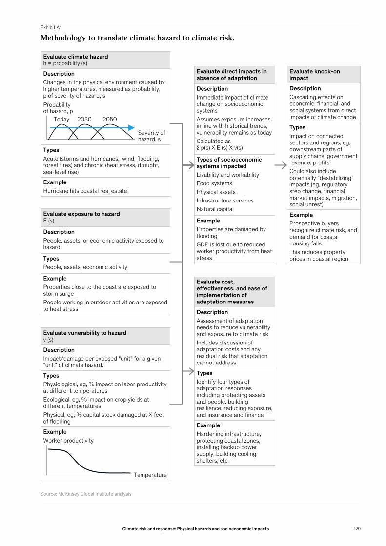
Exhibit A1
Methodology to translate climate hazard to climate risk.
Evaluate climate hazardh = probability (s)
DescriptionChanges in the physical environment caused by higher temperatures, measured as probability, p of severity of hazard, s
TypesAcute (storms and hurricanes, wind, flooding, forest fires) and chronic (heat stress, drought, sea-level rise)
ExampleHurricane hits coastal real estate
Evaluate exposure to hazardE (s)
DescriptionPeople, assets, or economic activity exposed to hazard
TypesPeople, assets, economic activity
ExampleProperties close to the coast are exposed to storm surgePeople working in outdoor activities are exposed to heat stress
Evaluate vunerability to hazardv (s)
DescriptionImpact/damage per exposed “unit” for a given “unit” of climate hazard.
TypesPhysiological, eg, % impact on labor productivity at different temperaturesEcological, eg, % impact on crop yields at different temperaturesPhysical, eg, % capital stock damaged at X feet of flooding
Example
Evaluate direct impacts in absence of adaptation
DescriptionImmediate impact of climate change on socioeconomic systemsAssumes exposure increases in line with historical trends, vulnerability remains as todayCalculated as Ʃ p(s) X E (s) X v(s)
Types of socioeconomic systems impactedLivability and workabilityFood systemsPhysical assetsInfrastructure servicesNatural capital
ExampleProperties are damaged by floodingGDP is lost due to reduced worker productivity from heat stress
Evaluate cost, effectiveness, and ease of implementation of adaptation measures
DescriptionAssessment of adaptation needs to reduce vulnerability and exposure to climate riskIncludes discussion of adaptation costs and any residual risk that adaptation cannot address
TypesIdentify four types of adaptation responses including protecting assets and people, building resilience, reducing exposure, and insurance and finance
ExampleHardening infrastructure, protecting coastal zones, installing backup power supply, building cooling shelters, etc
Evaluate knock-on impact
DescriptionCascading effects on economic, financial, and social systems from direct impacts of climate change
TypesImpact on connected sectors and regions, eg, downstream parts of supply chains, government revenue, profitsCould also include potentially “destabilizing” impacts (eg, regulatory step change, financial market impacts, migration, social unrest)
ExampleProspective buyers recognize climate risk, and demand for coastal housing fallsThis reduces property prices in coastal region
Source: McKinsey Global Institute analysis
Probability of hazard, p
Severity of hazard, s
Today 2030 2050
Worker productivity
Temperature
129Climate risk and response: Physical hazards and socioeconomic impacts
How we selected our case studies and performed the global geospatial risk analysisIn order to link physical climate risk to socioeconomic impact, we investigate nine specific cases that illustrate exposure to climate change extremes and proximity to physical thresholds. To select our case studies, we considered over 30 potential combinations of climate hazards, sectors, and geographies based on a review of the literature and expert interviews on the potential direct impacts of physical climate hazards. We find these hazards affect five different key socioeconomic systems: livability and workability, food systems, physical assets, infrastructure services, and natural capital. We ultimately chose nine cases to reflect these systems and based on their exposure to the extremes of climate change and their proximity today to key physiological, human-made, and ecological thresholds. As such, these cases represent leading-edge examples of climate change risk. For each case, we used the approach described above to quantify the inherent direct and knock-on risk from climate change, as well as outline a possible adaptation response.
For the global geospatial risk assessment, we began with the full set of 195 member countries of the United Nations, and then removed 90 of those due to their small geographic size, in order to account for the fact that GCMs' predictive skill decreases with spatial resolution. Therefore, we analyzed 105 countries against six indicators that cover the five socio-economic systems impact by climate change (Exhibit A2–A7).21 We did this using geospatial data on climate hazards (including a probabilistic assessment of the severity of the hazard and the likelihood of occurrence of events of different severity), exposure, and resilience. For example, we evaluated the potential for physical asset destruction by assessing the likelihood of floods of different severity and multiplied that against capital stock exposed to the flooding and the share of capital stock that could be damaged at different flood severities. We then added these up across different flood events to arrive at an annual expected damage number (that is, a probability-weighted assessment of possible impact). Note that this analysis provides an estimate only of the direct impact of physical climate risk and not the knock-on effects. These country-level analyses were then added up, where possible, in order to derive global insights about the evolution and distribution of various forms of climate risk.
A detailed discussion of the indicators used in the assessment is provided in Chapter 4 of the report. Here we primarily discuss the details of the hazard data used in the analysis, and climate models used in the analysis. We examined a subset of possible climate hazards, defining and measuring them as follows:
Lethal heat waves are defined as three-day events during which average daily maximum “wet-bulb” temperature could exceed the survivability threshold for a healthy human being resting in the shade. (Wet-bulb temperature is the lowest temperature to which air can be cooled by the evaporation of water into the air at a constant pressure.) We took the average wet-bulb temperature of the hottest six-hour period across each rolling three-day period as the relevant threshold. This was calculated according to the methodology in Stull (2011).22 The threshold maximum temperature chosen for this analysis was 34 degrees Celsius wet-bulb because the commonly defined heat threshold for human survivability is 35 degrees wet-bulb. At this temperature, a healthy human being, resting in the shade, can survive outdoors for four to five hours. Large cities with significant urban heat island effects could push 34 degrees Celsius wet-bulb heat waves over the 35-degree threshold. This could lead to widespread mortality in the absence of targeted adaptation.23 The lethal heatwave projections were derived from the CMIP5 multimodel ensemble, where each model was independently bias-
21 The indicators include: share of annual GDP at risk due to extreme heat and share of people at mortality risk due to lethal heat waves (measures of decrease in workability and livability), expected value of cereal production at risk of agricultural failure (measure of disruption of food systems), capital stock at risk of damage from floods, and share of a given decade spent in drought and land area experiencing biome shift (measures of destruction of natural capital).
22 R. Stull, 'Wet-bulb Temperature from Relative Humidity and Air Temperature," Journal of Applied Meteorology and Climatology, November 2011, Volume 50, pp. 2267–69.
23 A healthy human being can survive exposure to 35C wet-bulb temperatures for roughly 5 hours, assuming they are well hydrated and resting in the shade. For more details, please see Steven C. Sherwood and Matthew Huber, "An adaptability limit to climate change due to heat stress," Proceedings of the National Academy of Sciences, May 2010, Volume 107, Number 21, pp. 9552–55.
130 McKinsey Global Institute

corrected using the ERA-Interim dataset.24 Specifically, the projected incidence of lethal heatwaves between the 2021–40 period were counted across 20 GCMs drawn from the CMIP5 ensemble and independently bias corrected. Because 20 single-year observations across 20 models provides a sample size of only 400 years of data, the sample size was bootstrapped out to 1,000 years. Once a robust statistical sample size was established, the projected annual probability of a lethal heatwave was identified for each specific location by treating each year as independent. To account for a bug in the arid land-atmosphere feedbacks in the MIROC family of models, the analysis was performed both with and without the MIROC models. The results were insensitive to their exclusion.25 We eventually excluded all grid cells where the annual likelihood of lethal heatwaves was less than 1 percent. These projections are subject to uncertainty related to the future behavior of atmospheric aerosols and urban heat island or cooling island effects. High levels of atmospheric aerosols provide a cooling effect that masks the risk. Atmospheric aerosols, or air pollution reflect a proportion of incoming sunlight and therefore artificially cool regions, reducing air temperatures.26
Today, the regions that are subject to non-zero risk of lethal heatwaves all have high prevalence of atmospheric aerosols (see India case for further details). However, the CMIP5 models have poor representation of observed atmospheric aerosols in those regions. As a result, if the CMIP5 results showed a non-zero probability of lethal heat waves in certain regions today, this was set to zero.
The other form of uncertainty relates to the urban heat island effect. A global analysis of 419 major cities showed that the average daytime temperature difference between urban areas and their immediate surroundings is +1.5 ± 1.2°C, with some outliers up to 7 degrees Celsuis warmer.27 Research has demonstrated that many cities in India exhibit a negative urban heat island intensity in summer—that is, during the hot pre-monsoon season, they are cooler than their surroundings. This cooling effect is due to both to atmospheric aerosols and the relatively high vegetation cover in cities compared to their surroundings, which contain largely barren lands that are converted to croplands only post-monsoon. While these findings apply to much of the Indian subcontinent, the authors found that many cities in the north of the country exhibit statistically significant positive urban heat island intensities. Because this area of the country is also projected to be the first to exhibit heat waves close to the 35-degree threshold and because a reduction in atmospheric aerosols could further reduce the artificial cooling effect currently underway, these cities are at risk of having 34-degree heat waves amplified to 35-degree heat waves.28
Annual share of effective outdoor working hours affected by extreme heat and humidity in climate exposed-regions is calculated using the average percentage of a given 12-hour workday lost in regions exposed to these hazards. Labor capacity is lost due to heat and humidity through two mechanisms: the first, because workers must take breaks to avoid heatstroke, and the second because the body will naturally limit physiological output in hot conditions by fatiguing itself in a process known as “self-limiting.” Temperature projections were likewise taken from the CMIP5 multimodel ensemble mean projection, again bias corrected using the ERA-Interim dataset. Conversion to lost working hours was done following the methodology of Dunne et al. (2013), using combined ISO heat-exposure standards corrected with empirical data from Foster et al. (2019).29 When deriving global GDP
24 Bias corrected using the LOCI method, according to: Jürg Schmidli et al., "Downscaling from GCM precipitation: A benchmark for dynamical and statistical downscaling methods," International Journal of Climatology, April 2006, Volume 26, Number 5, p. 679–89.
25 Geert Jan Van Oldenborgh et al., "Extreme heat in India and anthropogenic climate change," Natural Hazards and Earth System Sciences, 2018, Volume 18, Number 1, pp. 365–81.
26 Geert Jan van Oldenborgh et al., “Extreme heat in India and anthropogenic climate change,” Natural Hazards and Earth System Sciences, 2018, Volume 18, Issue 1.
27 Shushi Peng et al., “Surface urban heat island across 419 global big cities,” Environmental Science & Technology, January 2012, Volume 46, Issue 2.
28 Hiteshri Shastri et al., “Flip flop of day-night and summer-winter surface urban heat island intensity in India,” Nature Scientific Reports, January 9, 2017, Volume 7.
29 John P. Dunne et al., "Reductions in labour capacity from heat stress under climate warming," Nature Climate Change, February 2013, Volume 3, pp. 563–66; Josh Foster et al., "A new paradigm to quantify reduction of physical work capacity in the heat," Medicine and Science in Sports and Exercise, 2019, Volume 51, Number 6, p. 15.
131Climate risk and response: Physical hazards and socioeconomic impacts
at risk, we applied lost working hours to GDP generated in sectors that we were confident are exposed to heat and humidity risk globally: agriculture, mining and quarrying, and construction. Lost working hours were applied one-to-one to sector GDP: that is, a projected X percent reduction in working hours is assumed to lead to an X percent reduction in sector GDP. These estimates are, as a result, likely an underestimate, as other sectors (particularly hospitality and tourism) are also exposed to heat. We considered a range based on the pace of sectoral transitions, ranging from keeping sector mix at today's level, to varying it going forward based on projections from IHS Markit Economics and Country Risk. To investigate the potential range of uncertainty around these findings, we explored the range of variability around the mean projection as captured by the ensemble model spread: we performed the same analysis using the 75th and 25th percentile ensemble projections. This was done to capture the potential impacts in an "average" year, compared with a "hotter than average" or "colder than average" year. Countries that include no change in share of effective outdoor working hours affected as a possible outcome within the range of model uncertainty by 2030 were noted as likely not robust. All countries show robust trends by 2050.
For our agricultural investigation, we used projections from the AgMIP ensemble. Changes in yield were quantified relative to the mean yield for the 1998–2017 period. Because projections from the AgMIP ensemble scale in skillfulness as a function of both physical spatial resolution and intensity of crop production, we were not able to perform a country-by-country analysis. (In other words, we were not able to obtain robust projections for small countries and large countries with marginal agricultural output.) Instead, we identified the largest grain breadbaskets in each region and quantified changes to output there. Agricultural projections were done using the mean projection from the full range of available GCMs, as well as the full range of non-potential-yield crop models. Nitrogen limitation and CO2 fertilization were kept “ON” for all projections. We did not account for reductions in nutritional content of crops. Therefore, these results may be underestimates, as future behavior of CO2 fertilization is not well constrained.
Water stress and change in water supply is calculated using the increase or decrease in the average annual supply of renewable freshwater available in a given water basin. The amount of available renewable freshwater is a function of annual precipitation over that basin, as well as influx and outflux of water to and from that basin via riverine systems. Water supply data were taken from the World Resources Institute, which combines output from the CMIP5 ensemble with the GLDAS-2 NOAH v. 3.3 hydrological model. Data was taken from the World Resources Institute Water Risk Atlas (2018), which relies on six underlying CMIP5 models. Time periods of this raw dataset are the 20-year periods centered on 2020, 2030, and 2040. The 1998–2017 and 2041–60 data were linearly extrapolated from the 60-year trend provided in the base dataset. For our global geospatial assessment across countries of water stress, we assumed water demand stayed constant at today's levels, to allow us to isolate and investigate the impact of climate change alone.
Our flooding hazard measure starts first by assessing the depth and spatial extent of a riverine flood event (measured in volume) for the full probability exceedance curve (100% to 0% chance) in a given year over the 1960–1999 period in a given 900-by-900-meter grid cell globally. This database was taken from the World Resources Institute, and a full methodology on its development is available on their website. This was then overlaid with data on precipitation changes, to approximate future flood hazards. This approach therefore should be considered to be only an approximation of the evolution of flooding hazard, and it should be noted that a more robust analysis of flooding will require the use of granular flood models. While the probability of extreme precipitation events is increasing over most of the world (due to the ability of warmer air to hold more water vapor than colder air), this increase is not uniform. Change in extreme precipitation probability was taken from a 1,000-year bootstrap of the CMIP5 multimodel ensemble, and then applied to the baseline flood data as a proxy for change in flood probability. When calculating capital stock at risk, the European Research Council’s global flood depth damage functions were applied to UNGAR15’s capital stock database. Existing flood protection for 1-in-50 to 1-in-100 year floods were assumed.
132 McKinsey Global Institute

Further limitations of this analysis include the focus on riverine flooding only (versus tidal, flash, or pluvial flooding, or flooding from storm surge), the ability to identify flood protections globally in a robust way and therefore adjust for today’s level of adaptation, and the ability to identify damage functions for capital stock that are specific to an individual site, such as a given building or a factory, rather than rely on more general damage functions.
Our drought hazard is calculated using the percentage of a given decade spent in drought conditions, where drought conditions are defined as a running three-month average where the self-calibrating Palmer Drought Severity Index value is less than -2. Drought data were taken from the CMIP5 multimodel ensemble mean projection and corrected for changes in biosphere behavior as a result of increases in atmospheric CO2.
Our measure of natural capital risk is defined as the percentage of land surface that changes category under the Köppen climate classification system, which evaluates a particular area based on average annual climate statistics, like precipitation and temperature. While not a perfect analogue, ecosystem type correlates very closely with Köppen climate classification, and therefore shifts are a good directional indicator of ecosystem stress or change.30
30 Our biome shift data were taken from Franz Rubel and Markus Kottek, “Observed and projected climate shifts 1901–2100 depicted by world maps of the Köppen-Geiger climate classification,” Meteorologische Zeitschrift (Contributions to Atmospheric Sciences), April 2010, Volume 19, Number 2.
133Climate risk and response: Physical hazards and socioeconomic impacts
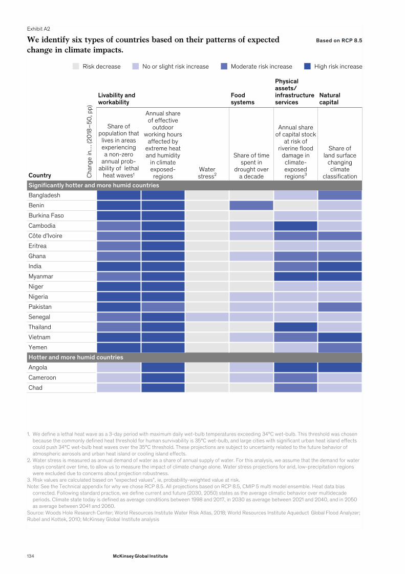
Exhibit A2
We identify six types of countries based on their patterns of expected change in climate impacts.
Source: Woods Hole Research Center; World Resources Institute Water Risk Atlas, 2018; World Resources Institute Aqueduct Global Flood Analyzer; Rubel and Kottek, 2010; McKinsey Global Institute analysis
1. We define a lethal heat wave as a 3-day period with maximum daily wet-bulb temperatures exceeding 34°C wet-bulb. This threshold was chosen because the commonly defined heat threshold for human survivability is 35°C wet-bulb, and large cities with significant urban heat island effects could push 34°C wet-bulb heat waves over the 35°C threshold. These projections are subject to uncertainty related to the future behavior of atmospheric aerosols and urban heat island or cooling island effects.
2. Water stress is measured as annual demand of water as a share of annual supply of water. For this analysis, we assume that the demand for water stays constant over time, to allow us to measure the impact of climate change alone. Water stress projections for arid, low-precipitation regions were excluded due to concerns about projection robustness.
3. Risk values are calculated based on “expected values”, ie, probability-weighted value at risk.Note: See the Technical appendix for why we chose RCP 8.5. All projections based on RCP 8.5, CMIP 5 multi model ensemble. Heat data bias
corrected. Following standard practice, we define current and future (2030, 2050) states as the average climatic behavior over multidecade periods. Climate state today is defined as average conditions between 1998 and 2017, in 2030 as average between 2021 and 2040, and in 2050 as average between 2041 and 2060.
Based on RCP 8.5
Livability and workability
Food systems
Physical assets/infrastructure services
Natural capital
Country
Share of population that
lives in areas experiencing a non-zero
annual prob-ability of lethal
heat waves1
Annual share of effective
outdoor working hours
affected by extreme heat and humidity
in climate exposed-regions
Waterstress2
Share of time spent in
drought over a decade
Annual share of capital stock
at risk of riverine flood
damage in climate-exposed regions3
Share of land surface
changing climate
classificationSignificantly hotter and more humid countriesBangladeshBeninBurkina FasoCambodiaCôte d’IvoireEritreaGhanaIndiaMyanmarNigerNigeriaPakistanSenegalThailandVietnamYemenHotter and more humid countriesAngolaCameroonChad
Chan
ge in
… (2
018–
50, p
p)
Risk decrease No or slight risk increase Moderate risk increase High risk increase
134 McKinsey Global Institute
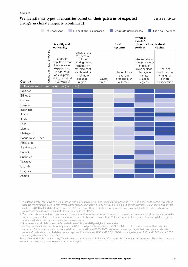
Exhibit A3
We identify six types of countries based on their patterns of expected change in climate impacts (continued).
Source: Woods Hole Research Center; World Resources Institute Water Risk Atlas, 2018; World Resources Institute Aqueduct Global Flood Analyzer; Rubel and Kottek, 2010; McKinsey Global Institute analysis
1. We define a lethal heat wave as a 3-day period with maximum daily wet-bulb temperatures exceeding 34°C wet-bulb. This threshold was chosen because the commonly defined heat threshold for human survivability is 35°C wet-bulb, and large cities with significant urban heat island effects could push 34°C wet-bulb heat waves over the 35°C threshold. These projections are subject to uncertainty related to the future behavior of atmospheric aerosols and urban heat island or cooling island effects.
2. Water stress is measured as annual demand of water as a share of annual supply of water. For this analysis, we assume that the demand for water stays constant over time, to allow us to measure the impact of climate change alone. Water stress projections for arid, low-precipitation regions were excluded due to concerns about projection robustness.
3. Risk values are calculated based on “expected values”, ie, probability-weighted value at risk.Note: See the Technical appendix for why we chose RCP 8.5. All projections based on RCP 8.5, CMIP 5 multi model ensemble. Heat data bias
corrected. Following standard practice, we define current and future (2030, 2050) states as the average climatic behavior over multidecade periods. Climate state today is defined as average conditions between 1998 and 2017, in 2030 as average between 2021 and 2040, and in 2050 as average between 2041 and 2060.
Based on RCP 8.5
Livability and workability
Food systems
Physical assets/infrastructure services
Natural capital
Country
Share of population that
lives in areas experiencing a non-zero
annual prob-ability of lethal
heat waves1
Annual share of effective
outdoor working hours
affected by extreme heat and humidity
in climate exposed-regions
Waterstress2
Share of time spent in
drought over a decade
Annual share of capital stock
at risk of riverine flood
damage in climate-exposed regions3
Share of land surface
changing climate
classificationHotter and more humid countries (continued)EcuadorEthiopiaGuineaGuyanaIndonesiaJapanJordanLaosLiberiaMadagascarPapua New GuineaPhilippinesSaudi ArabiaSomaliaSurinameTanzaniaUgandaUruguayZambia
Chan
ge in
… (2
018–
50, p
p)
Risk decrease No or slight risk increase Moderate risk increase High risk increase
135Climate risk and response: Physical hazards and socioeconomic impacts

Exhibit A4
We identify six types of countries based on their patterns of expected change in climate impacts (continued).
Source: Woods Hole Research Center; World Resources Institute Water Risk Atlas, 2018; World Resources Institute Aqueduct Global Flood Analyzer; Rubel and Kottek, 2010; McKinsey Global Institute analysis
1. We define a lethal heat wave as a 3-day period with maximum daily wet-bulb temperatures exceeding 34°C wet-bulb. This threshold was chosen because the commonly defined heat threshold for human survivability is 35°C wet-bulb, and large cities with significant urban heat island effects could push 34°C wet-bulb heat waves over the 35°C threshold. These projections are subject to uncertainty related to the future behavior of atmospheric aerosols and urban heat island or cooling island effects.
2. Water stress is measured as annual demand of water as a share of annual supply of water. For this analysis, we assume that the demand for water stays constant over time, to allow us to measure the impact of climate change alone. Water stress projections for arid, low-precipitation regions were excluded due to concerns about projection robustness.
3. Risk values are calculated based on “expected values”, ie, probability-weighted value at risk.Note: See the Technical appendix for why we chose RCP 8.5. All projections based on RCP 8.5, CMIP 5 multi model ensemble. Heat data bias
corrected. Following standard practice, we define current and future (2030, 2050) states as the average climatic behavior over multidecade periods. Climate state today is defined as average conditions between 1998 and 2017, in 2030 as average between 2021 and 2040, and in 2050 as average between 2041 and 2060.
Based on RCP 8.5
Livability and workability
Food systems
Physical assets/infrastructure services
Natural capital
Country
Share of population that
lives in areas experiencing a non-zero
annual prob-ability of lethal
heat waves1
Annual share of effective
outdoor working hours
affected by extreme heat and humidity
in climate exposed-regions
Waterstress2
Share of time spent in
drought over a decade
Annual share of capital stock
at risk of riverine flood
damage in climate-exposed regions3
Share of land surface
changing climate
classificationHotter countriesBotswanaCentral African Rep.ColombiaCubaDem. Rep. CongoGabonGuatemalaHondurasHungaryLibyaMalawiMalaysiaMaliMauritaniaMozambiqueNamibiaNicaraguaOmanParaguayRep. CongoRomaniaSerbia
Chan
ge in
… (2
018–
50, p
p)
Risk decrease No or slight risk increase Moderate risk increase High risk increase
136 McKinsey Global Institute
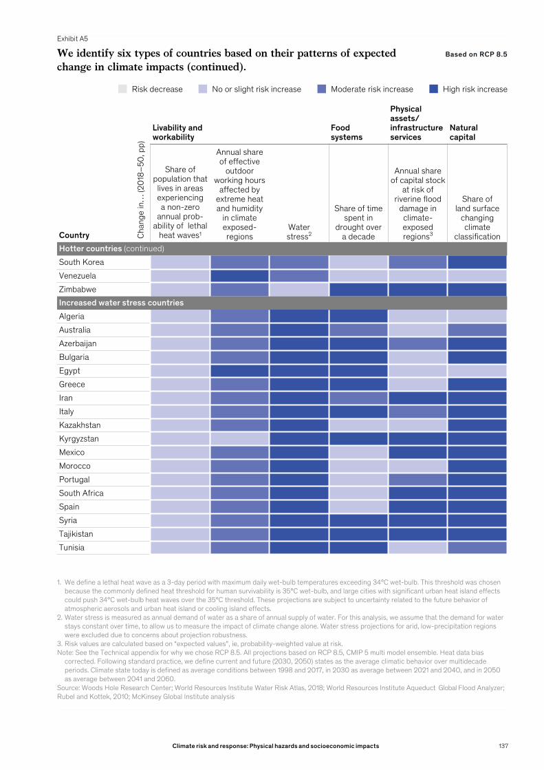
Exhibit A5
We identify six types of countries based on their patterns of expected change in climate impacts (continued).
Source: Woods Hole Research Center; World Resources Institute Water Risk Atlas, 2018; World Resources Institute Aqueduct Global Flood Analyzer; Rubel and Kottek, 2010; McKinsey Global Institute analysis
1. We define a lethal heat wave as a 3-day period with maximum daily wet-bulb temperatures exceeding 34°C wet-bulb. This threshold was chosen because the commonly defined heat threshold for human survivability is 35°C wet-bulb, and large cities with significant urban heat island effects could push 34°C wet-bulb heat waves over the 35°C threshold. These projections are subject to uncertainty related to the future behavior of atmospheric aerosols and urban heat island or cooling island effects.
2. Water stress is measured as annual demand of water as a share of annual supply of water. For this analysis, we assume that the demand for water stays constant over time, to allow us to measure the impact of climate change alone. Water stress projections for arid, low-precipitation regions were excluded due to concerns about projection robustness.
3. Risk values are calculated based on “expected values”, ie, probability-weighted value at risk.Note: See the Technical appendix for why we chose RCP 8.5. All projections based on RCP 8.5, CMIP 5 multi model ensemble. Heat data bias
corrected. Following standard practice, we define current and future (2030, 2050) states as the average climatic behavior over multidecade periods. Climate state today is defined as average conditions between 1998 and 2017, in 2030 as average between 2021 and 2040, and in 2050 as average between 2041 and 2060.
Based on RCP 8.5
Livability and workability
Food systems
Physical assets/infrastructure services
Natural capital
Country
Share of population that
lives in areas experiencing a non-zero
annual prob-ability of lethal
heat waves1
Annual share of effective
outdoor working hours
affected by extreme heat and humidity
in climate exposed-regions
Waterstress2
Share of time spent in
drought over a decade
Annual share of capital stock
at risk of riverine flood
damage in climate-exposed regions3
Share of land surface
changing climate
classificationHotter countries (continued)South KoreaVenezuelaZimbabweIncreased water stress countriesAlgeriaAustraliaAzerbaijanBulgariaEgyptGreeceIranItalyKazakhstanKyrgyzstanMexicoMoroccoPortugalSouth AfricaSpainSyriaTajikistanTunisia
Chan
ge in
… (2
018–
50, p
p)
Risk decrease No or slight risk increase Moderate risk increase High risk increase
137Climate risk and response: Physical hazards and socioeconomic impacts

Exhibit A6
We identify six types of countries based on their patterns of expected change in climate impacts (continued).
Source: Woods Hole Research Center; World Resources Institute Water Risk Atlas, 2018; World Resources Institute Aqueduct Global Flood Analyzer; Rubel and Kottek, 2010; McKinsey Global Institute analysis
1. We define a lethal heat wave as a 3-day period with maximum daily wet-bulb temperatures exceeding 34°C wet-bulb. This threshold was chosen because the commonly defined heat threshold for human survivability is 35°C wet-bulb, and large cities with significant urban heat island effects could push 34°C wet-bulb heat waves over the 35°C threshold. These projections are subject to uncertainty related to the future behavior of atmospheric aerosols and urban heat island or cooling island effects.
2. Water stress is measured as annual demand of water as a share of annual supply of water. For this analysis, we assume that the demand for water stays constant over time, to allow us to measure the impact of climate change alone. Water stress projections for arid, low-precipitation regions were excluded due to concerns about projection robustness.
3. Risk values are calculated based on “expected values”, ie, probability-weighted value at risk.Note: See the Technical appendix for why we chose RCP 8.5. All projections based on RCP 8.5, CMIP 5 multi model ensemble. Heat data bias
corrected. Following standard practice, we define current and future (2030, 2050) states as the average climatic behavior over multidecade periods. Climate state today is defined as average conditions between 1998 and 2017, in 2030 as average between 2021 and 2040, and in 2050 as average between 2041 and 2060.
Based on RCP 8.5
Livability and workability
Food systems
Physical assets/infrastructure services
Natural capital
Country
Share of population that
lives in areas experiencing a non-zero
annual prob-ability of lethal
heat waves1
Annual share of effective
outdoor working hours
affected by extreme heat and humidity
in climate exposed-regions
Waterstress2
Share of time spent in
drought over a decade
Annual share of capital stock
at risk of riverine flood
damage in climate-exposed regions3
Share of land surface
changing climate
classificationIncreased water stress countries (continued)TurkeyTurkmenistanUkraineUzbekistanLower-risk countriesAustriaBelarusCanadaFinlandFranceGermanyIcelandMongoliaNew ZealandNorwayPeruPolandRussiaSwedenUnited Kingdom
Chan
ge in
… (2
018–
50, p
p)
Risk decrease No or slight risk increase Moderate risk increase High risk increase
138 McKinsey Global Institute

Exhibit A7
We identify six types of countries based on their patterns of expected change in climate impacts (continued).
Source: Woods Hole Research Center; World Resources Institute Water Risk Atlas, 2018; World Resources Institute Aqueduct Global Flood Analyzer; Rubel and Kottek, 2010; McKinsey Global Institute analysis
1. We define a lethal heat wave as a 3-day period with maximum daily wet-bulb temperatures exceeding 34°C wet-bulb. This threshold was chosen because the commonly defined heat threshold for human survivability is 35°C wet-bulb, and large cities with significant urban heat island effects could push 34°C wet-bulb heat waves over the 35°C threshold. These projections are subject to uncertainty related to the future behavior of atmospheric aerosols and urban heat island or cooling island effects.
2. Water stress is measured as annual demand of water as a share of annual supply of water. For this analysis, we assume that the demand for water stays constant over time, to allow us to measure the impact of climate change alone. Water stress projections for arid, low-precipitation regions were excluded due to concerns about projection robustness.
3. Risk values are calculated based on “expected values”, ie, probability-weighted value at risk.4. Calculated assuming constant exposure. Constant exposure means that we do not factor in any increases in population or assets, or shifts in the
spatial mix of population and assets. This was done to allow us to isolate the impact of climate change alone. Color coding for each column based on the spread observed across countries within the indicator.
Note: See the Technical appendix for why we chose RCP 8.5. All projections based on RCP 8.5, CMIP 5 multi model ensemble. Heat data bias corrected. Following standard practice, we define current and future (2030, 2050) states as the average climatic behavior over multidecade periods. Climate state today is defined as average conditions between 1998 and 2017, in 2030 as average between 2021 and 2040, and in 2050 as average between 2041 and 2060.
Based on RCP 8.5
Livability and workability
Food systems
Physical assets/infrastructure services
Natural capital
Country
Share of population that
lives in areas experiencing a non-zero
annual prob-ability of lethal
heat waves1
Annual share of effective
outdoor working hours
affected by extreme heat and humidity
in climate exposed-regions
Waterstress2
Share of time spent in
drought over a decade
Annual share of capital stock
at risk of riverine flood
damage in climate-exposed regions3
Share of land surface
changing climate
classificationDiverse climate countriesArgentinaBrazilChileChinaUnited States
Change in potential impact, 2018–504 (percentage points)Risk decrease n/a n/a <0 <0 <0 n/aNo or slight risk increase 0–0.5 0–0.5 0–3 0–3 0–0.05 0–5Moderate risk increase 0.5–5.0 0.5–5.0 3–7 3–7 0.05–0.10 5–10High risk increase >5.0 >5.0 >7 >7 >0.10 >10
Chan
ge in
… (2
018–
50, p
p)
Risk decrease No or slight risk increase Moderate risk increase High risk increase
139Climate risk and response: Physical hazards and socioeconomic impacts
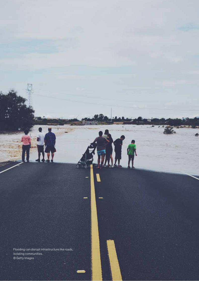
Flooding can disrupt infrastructure like roads, isolating communities. © Getty Images

Bibliography
Reports
Alexandratos, Nikos, and Jelle Bruinsma, World agriculture towards 2030/2050: The 2012 revision, ESA working paper number 12-03, Agricultural Development Economics Division, Food and Agriculture Organization of the United Nations, June 2012.
Allianz, Allianz Risk Barometer 2019, January 2019.
Bank of England, Climate change: What are the risks to financial stability? November 2017.
Bapna, Manish et al., Adapt now: A global call for leadership on climate resilience, Global Commission on Adaptation, September 2019.
Brody, Sarah, Matt Rogers, and Giulia Siccardo, “Why, and how, utilities should start to manage climate-change risk,” April 2019, McKinsey.com.
Brumbaugh, Robert, Healthy coral reefs are good for tourism—and tourism can be good for reefs, World Economic Forum, June 21, 2017.
Ciscar, Juan Carlos et al., Climate impacts in Europe: Final report of the JRC PESETA III project, European Commission, 2018; “Peseta II,” European Commission.
Eis, Jason et al., Changing course: A comprehensive investor guide to scenario-based methods for climate risk assessment, in response to the TCFD, UNEP Finance Initiative, May 2019.
European Commission, Forest fires: Sparking firesmart policies in the EU, November 2018.
European Commission, Green infrastructure implementation: Proceedings of the EC Conference 19 November 2010, Brussels, Belgium, February 2011.
European Environmental Agency, What is green infrastructure? March 29, 2017.
FAO, Global forest resources assessment 2010, 2010, FAO forestry paper number 163.
FAO, The state of food security and nutrition in the world 2018: Building climate resilience for food security and nutrition, 2018.
FAO, The state of the world’s forests: Forest pathways to sustainable development, 2018.
FAO, The state of world fisheries and aquaculture 2012, 2012, fao.org/3/a-i2727e.pdf.
FAO, “What happened to world food prices and why?,” in The state of agricultural commodity markets 2009, 2009.
Global Infrastructure Hub and Oxford Economics, Global infrastructure outlook, 2017.
Hallegatte, Stephane, Jun Rentschler, and Julie Rozenberg, Lifelines: The Resilient Infrastructure Opportunity, Washington, DC: World Bank, July 2019.
Hennemuth, Barbara et al., Statistical methods for the analysis of simulated and observed climate data: Applied in projects and institutions dealing with climate change impact and adaptation, Climate Service Center, CSC report number 13, 2013.
Hindlian, Amanda et al., Taking the heat: Making cities resilient to climate change, Goldman Sachs Global Markets Institute, September 2019.
Hughes, Gordon, Paul Chinowsky, and Ken Strzepek, The costs of adapting to climate change for infrastructure, World Bank, 2007.
Intergovernmental Panel on Climate Change (IPCC), Climate change 2014: Synthesis report, 2014.
IPCC, Special report: Global warming of 1.5°C, 2018.
Kumari Rigaud, Kanta et al., Groundswell: Preparing for internal climate migration, World Bank, March 2018.
Mahalingam, A. et al., Impacts of severe natural catastrophes on financial markets, Cambridge Centre for Risk Studies, 2018.
McKinsey Global Institute, Bridging global infrastructure gaps, June 2016.
McKinsey Global Institute, Bridging infrastructure gaps: Has the world made progress? 2017.
McKinsey Global Institute, Globalization in transition: The future of trade and value chains, January 2019.
McKinsey Global Institute, Superstars: The firms, sectors, and cities leading the global economy, October 2018.
McKinsey (2017) “Digital Economy - A guide to transforming the economy”.
141Climate risk and response: Physical hazards and socioeconomic impacts
National Oceanic and Atmospheric Administration (NOAA) and US Census Bureau, National coastal population report: Population trends from 1970 to 2020, March 2013.
NOAA National Hurricane Center, “Costliest U.S. tropical cyclones tables updated,” January 26, 2018.
NOAA National Centers for Environmental Information, Billion-dollar weather and climate disasters: Overview, 2019.
Ocean Acidification International Coordination Centre, “Ocean acidification in the IPCC Special Report: Global warming of 1.5°C,” October 8, 2018.
OECD and FAO, OECD-FAO Agricultural Outlook 2018–2027, 2018.
Olhoff, Anne et al., The adaptation finance gap report, UNEP DTU Partnership, 2016.
Parry, Martin et al., Assessing the costs of adaption to climate change: A review of the UNFCCC and other recent estimates, International Institute for Environment and Development and Grantham Institute for Climate Change, August 2009.
Resilinc, EventWatch 2018 annual report, 2019.
Stern, Nicholas, The Economics of Climate Change: The Stern Review, Cambridge, UK: Cambridge University Press, 2007.
Task Force on Climate-related Financial Disclosures, Final report: Recommendations of the Task Force on Climate-related Financial Disclosures, June 2017.
UN Environment Programme, The adaptation gap report 2018, 2018.
United States Agency for International Development, Addressing climate change impacts on infrastructure: Preparing for change, November 2012, revised December 2013.
US Global Change Research Program, Fourth national climate assessment, 2017–18.
World Bank, Economics of adaptation to climate change: Synthesis report, 2010.
World Climate Research Programme, CMIP Phase 5 (CMIP5), wrp-climate.org/wgcm-cmip/wgcm-cmip5.
Papers in scientific journals
Ahern, Mike et al., “Global health impacts of floods: Epidemological evidence,” Epidemiologic Reviews, July 2005, Volume 27, Issue 1.
Allen, Myles R. et al., “Warming caused by cumulative carbon emissions towards the trillionth tonne,” Nature, April 2009, Volume 458, Issue 7242.
Archer, David, “The fate of fossil fuel CO2 in geologic time,” Journal of Geophysical Research: Oceans, September 2005, Volume 110, Issue C9.
Arias-Ortiz, A. et al., “A marine heat wave drives massive losses from the world’s largest seagrass carbon stocks,” Nature, March 2018, Volume 8.
Armstrong, Scott B. et al., “Indications of a positive feedback between coastal development and beach nourishment,” Earth’s Future, December 2016, Volume 4, Issue 12.
Asseng, Senthold et al., “Can Egypt become self-sufficient in wheat?,” Environmental Research Letters, September 2018, Volume 13, Number 9.
Bangalore, Mook, Andrew Smith, and Ted Veldkamp, “Exposure to floods, climate change, and poverty in Vietnam,” Economics of Disasters and Climate Change, April 2019, Volume 3, Issue 1.
Barthel, Fabian, and Eric Neumayer, “A trend analysis of normalized insured damage from natural disasters,” Climatic Change, July 2012, Volume 113, Issue 2.
Bastin, Jean-Francois et al, “Understanding climate change from a global analysis of city analogues,” PLOS ONE, July 2019, Volume 14, Number 7.
Ben-Ari, Tamara et al., “Causes and implications of the unforeseen 2016 extreme yield loss in the breadbasket of France,” Nature Communications, April 2018, Volume 9, Article 1627.
Beniston, Martin, “Impacts of climatic change on water and associated economic activities in the Swiss Alps,” Journal of Hydrology, January 2012, Volumes 412–413.
Bereiter, Bernhard et al., “Revision of the EPICA Dome C CO2 record from 800 to 600 kyr before present,” Geophysical Research Letters, January 2015, Volume 42, Issue 2.
Bernstein, Asaf, Matthew T. Gustafson, and Ryan Lewis, “Disaster on the horizon: The price effect of sea level rise,” Journal of Financial Economics, November 2019, Volume 134, Issue 2.
142 McKinsey Global Institute

Bevacqua, E. et al., “Higher probability of compound flooding from precipitation and storm surge in Europe under anthropogenic climate change,” Science Advances, September 19, Volume 5, Issue 9.
Bhattacharya, Shaoni, “Deadly new wheat disease threatens Europe’s crops,” Nature, February 2017, Volume 542, Issue 7640.
Blasiak, Robert et al., “Climate change and marine fisheries: Least developed countries top global index of vulnerability,” PLOS ONE, June 2017, Volume 12, Number 6.
Bobenrieth, Eugenio et al., “Stocks-to-use ratios and prices as indicators of vulnerability to spikes in global cereal markets,” Agricultural Economics, February 2013, Volume 44, supplement 43–52.
Bonthuys, Jorisna, “Cape Town drought places sewerage systems under pressure,” Water Wheel, May 2018, Volume 17, Number 3.
Brode, Peter et al., “Estimated work ability in warm outdoor environments depends on the chosen heat stress assessment metric,” International Journal of Biometeorology, April 2017, Issue 62.
Bunn, Christian et al., “A bitter cup: Climate change profile of global production of Arabica and Robusta coffee,” Climatic Change, March 2015, Volume 129, Issue 1–2.
Burgess, Seth D., Samuel Bowring, and Shu-zhong Shen, “High-precision timeline for Earth’s most severe extinction,” Proceedings of the National Academy of Sciences, March 2014, Volume 111, Number 9.
Burkett, Virginia R. et al., “Nonlinear dynamics in ecosystem response to climatic change: Case studies and policy implications,” Ecological Complexity, December 2005, Volume 2, Issue 4.
Bynum, Gaither D. et al., “Induced hyperthermia in sedated humans and the concept of a critical thermal maximum,” American Journal of Physiology, November 1978, Volume 235, Issue 5.
Carey, Mark, “Disasters, development, and glacial lake control in twentieth-century Peru,” in Mountains: Sources of Water, Sources of Knowledge, Ellen Wiegandt, ed., Springer, 2008.
Chadburn, S. E. et al., “An observation-based constraint on permafrost loss as a function of global warming,” Nature Climate Change, May 2017, Volume 7, Issue 5.
Chaturvedi, Vaibhav, and Monit Sharma, “Modelling long-term HFC emissions from India’s residential air-conditioning sector: Exploring implications of alternative refrigerants, best practices, and a sustainable lifestyle within an integrated assessment modelling framework,” Climate Policy, 2016, Volume 16, Issue 7.
Chen, Jie et al., “Bias correcting climate model multi-member ensembles to assess climate change impacts on hydrology,” Climatic Change, April 2019, Volume 153, Issue 3.
Coffel, E., and R. Horton, “Climate change and the impact of extreme temperatures on aviation,” Weather, Climate, and Society, January 2015, Volume 7, Number 1.
Coffel, Ethan D., Terence R. Thompson, and Radley M. Horton, “The impacts of rising temperatures on aircraft takeoff performance,” Climatic Change, September 2017, Volume 144, Issue 2.
Cramer, Wolfgang et al., “Climate change and interconnected risks to sustainable development in the Mediterranean,” Nature Climate Change, November 2018, Volume 8, Issue 11.
Cross, John A., “Megacities and small towns: Different perspectives on hazard vulnerability,” Global Environmental Change Part B: Environmental Hazards, June 2001, Volume 3, Issue 2.
Dale, Virginia H. et al., “Climate change and forest disturbances,” BioScience, September 2001, Volume 51, Issue 9.
Davy, Richard, Linling Chen, and Edward Hanna, “Arctic amplification metrics,” International Journal of Climatology, October 2018, Volume 38, Issue 12.
DeConto, Robert M., and David Pollard, “Contribution of Antarctica to past and future sea-level rise,” Nature, March 2016, Volume 531, Issue 7596.
Dessens, Jean, Claude Berthet, and J. L. Sanchez, “Change in hailstone size distributions with an increase in the melting level height,” Atmospheric Research, May 2015, Volume 158–9.
Dietz, Simon et al., “‘Climate value at risk’ of global financial assets,” Nature Climate Change, April 2016, Volume 6.
Diffenbaugh, Noah S., and Christopher B. Field, “Changes in ecologically critical terrestrial climate conditions,” Science, August 2013, Volume 341, Issue 6145.
Diffenbaugh, Noah S. et al., “Robust increases in severe thunderstorm environments in response to greenhouse forcing,” Proceedings of the National Academy of Sciences, October 2013, Volume 10, Number 41.
Döll, Petra et al., “Risks for the global freshwater system at 1.5°C and 2°C global warming,” Environmental Research Letters, April 2018, Volume 13, Number 4.
Efron, Beran, “Bootstrap methods: Another look at the jackknife,” The Annals of Statistics, January 1979, Volume 7, Number 1.
143Climate risk and response: Physical hazards and socioeconomic impacts

Feynman, Joan, and Alexander Ruzmaikin, “Climate stability and the origin of agriculture,” in Climate Change and Agriculture, Saddam Hussain, ed., IntechOpen, 2018.
Flato, Gregory et al., “Evaluation of climate models,” in Climate Change 2013: The Physical Science Basis: Contribution of Working Group I to the Fifth Assessment Report of the Intergovernmental Panel on Climate Change, Thomas F. Stocker et al., eds., New York, NY: Cambridge University Press, 2014.
Fraga, Helder et al., “Modelling climate change impacts on viticultural yield, phenology and stress conditions in Europe,” Global Change Biology, November 2016, Volume 22, Issue 11.
Free, Christopher M. et al., “Impacts of historical warming on marine fisheries production,” Science, March 2019, Volume 363, Issue 6430.
Friedlingstein, Pierre et al., “Uncertainties in CMIP5 climate projections due to carbon cycle feedbacks,” Journal of Climate, January 2014, Volume 27, Number 2.
Frölicher, Thomas L., Erich M. Fischer, and Nicolas Gruber, “Marine heat waves under global warming,” Nature, August 2018, Volume 560.
Fry, Jillian P. et al., “Feed conversion efficiency in aquaculture: Do we measure it correctly?,” Environmental Research Letters, 2018, Volume 13, Number 2.
Gallagher, Justin, and Daniel Hartley, “Household finance after a natural disaster: The case of Hurricane Katrina,” August 2017, American Economic Journal: Economic Policy, Volume 9, Number 3.
Galassi, Gaia, and Spada, Giorgio, “Sea-level rise in the Mediterranean Sea by 2050: Roles of terrestrial ice melt, steric effects and glacial isostatic adjustment,” Global and Planetary Change, 2014, Volume 123.
Gautam, Raina, and Sunanda, Sinha, “Outlook on the Indian scenario of solar energy strategies: Policies and challenges,” Energy Strategy Reviews, 2019, Volume 24.
Grotch, Stanley L., and Michael C. MacCracken, “The use of general circulation models to predict regional climatic change,” Journal of Climate, March 1991, Volume 4, Number 3.
Guerry, Anne D. et al., “Natural capital and ecosystem services informing decisions: From promise to practice,” Proceedings of the National Academy of Sciences, June 2015, Volume 112, Number 24.
Haeberli, Wilfried, Yvonne Schaub, and Christian Huggel, “Increasing risks related to landslides from degrading permafrost into new lakes in de-glaciating mountain ranges,” Geomorphology, September 2017, Volume 293, Part B.
Haghighi, Erfan, Kaveh Madani, and Arjen Y. Hoekstra, “The water footprint of water conservation using shade balls in California,” Nature Sustainability, July 2018, Volume 1, Issue 7.
Halpern, Benjamin et al., Cumulative human impacts: Raw stressor data (2008 and 2013), Knowledge Network for Biocomplexity, 2015.
Hancock, P. A., and Ioannis Vasmatzidis, “Human occupational performance limits under stress: The thermal environment as a prototypical example,” Ergonomics, 1998, Volume 41, Issue 8.
Hannah, Lee et al., “Climate change, wine, and conservation,” Proceedings of the National Academy of Sciences, April 2013, Volume 110, Number 17.
Hanson, Susan et al., “A global ranking of port cities with high exposure to climate extremes,” Climatic Change, January 2011, Volume 104, Issue 1.
Haque, Nawshad et al., “Rare earth elements: Overview of mining, mineralogy, uses, sustainability and environmental impact,” Resources, October 2014, Volume 3, Issue 4.
Haraguchi, Masahiko, and Upmanu Lall, “Flood risks and impacts: A case study of Thailand’s floods in 2011 and research questions for supply chain decision making,” International Journal of Disaster Risk Reduction, December 2015, Volume 14, Part 3.
Harrison, Sandy P., Patrick J. Bartlein, and I. Colin Prentice, “What have we learnt from paleoclimate simulations?,” Journal of Quaternary Science, May 2016, Volume 31, Issue 4.
Hasselmann, Klaus, “Is climate predictable?,” in The Science of Disasters: Climate Disruptions, Heart Attacks, and Market Crashes, Armin Bunde, Jürgen Kropp, and Hans Joachim Schellnhuber, eds., Berlin, Germany: Springer, 2002.
Hausfather, Zeke et al., “Assessing recent warming using instrumentally homogeneous sea surface temperature records,” Science Advances, January 2017, Volume 3, Number 1.
Hawkins, Ed, and Rowan Sutton, “The potential to narrow uncertainty in regional climate predictions,” Bulletin of the American Meteorological Society, August 2009, Volume 90, Number 8.
Heller, Nicole E. and Zavaleta, Erika S., “Biodiversity management in the face of climate change: a review of 22 years of recommendations,” Biological conservation, 2009, Volume 142.
Henneaux, Pierre, “Probability of failure of overloaded lines in cascading failures,” Electrical Power & Energy Systems, December 2015, Volume 73.
Hock, Regine et al., “GlacierMIP – A model intercomparison of global-scale glacier mass-balance models and projections,” Journal of Glaciology, June 2019, Volume 65, Issue 251.
144 McKinsey Global Institute
Hoegh-Guldberg, Ove et al., “The ocean,” in Climate Change 2014: Impacts, Adaptation, and Vulnerability, Part B: Regional Aspects, Intergovernmental Panel on Climate Change, New York, NY: Cambridge University Press, 2014.
Houghton, Richard A., and Joseph L. Hackler, Carbon flux to the atmosphere from land-use changes: 1850 to 2005, Carbon Dioxide Information Analysis Center, Oak Ridge National Laboratory, US Department of Energy, 2001.
Hsiang, Solomon et al., “Estimating economic damage from climate change in the United States,” Science, June 30, 2017, Volume 356, Issue 6345.
Hu, Xi et al., “The spatial exposure of the Chinese infrastructure system to flooding and drought hazards,” Natural Hazards, January 2016, Volume 80.
Huber, Markus, and Reto Knutti, “Anthropogenic and natural warming inferred from changes in Earth’s energy balance,” Nature Geoscience, December 2011, Volume 5.
Hughes, Terry P. et al., “Global warming and recurrent mass bleaching of corals,” Nature, March 2017, Volume 543.
Hughes, Terry P. et al., “Global warming impairs stock—recruitment dynamics of corals,” Nature, April 2019, Volume 568.
Hughes, Terry P. et al., “Global warming transforms coral reef assemblages,” Nature, April 2018, Volume 556.
Huss, Matthias, and Regine Hock, “Global-scale hydrological response to future glacier mass loss,” Nature Climate Change, January 2018, Volume 8, Number 2.
Im, Eun-Soon, Jeremy S. Pal, and Elfatih A. B. Eltahir, “Deadly heat waves projected in the densely populated agricultural regions of South Asia,” Science Advances, August 2, 2017, Volume 3, Number 8.
India State-Level Disease Burden Initiative Air Pollution Collaborators, “The impact of air pollution in deaths, disease burden, and life expectancy across the states of India: The Global Burden of Disease Study 2017,” Lancet Planetary Health, January 2019, Volume 3, Issue 1.
Irish, Jennifer L. et al., “Simulation of Hurricane Katrina (2005) under sea level and climate conditions for 1900,” Climatic Change, February 2014, Volume 122, Issue 4.
Iturrizaga L., “Glacier Lake Outburst Floods”, Encyclopedia of Snow, Ice and Glaciers, 2011.
Ivanov, Martin Aleksandrov, Jürg Luterbacher, and Sven Kotlarski, “Climate model biases and modification of the climate change signal by intensity-dependent bias correction,” Journal of Climate, August 2018, Volume 31, Number 16.
James, Rachel et al., “Evaluating climate models with an African lens,” Bulletin of the American Meteorological Society, February 2018, Volume 99, Number 2.
Jones, Gregory V. et al., “Climate change and global wine quality,” Climate Change, December 2005, Volume 73, Issue 3.
Juroszek, Peter, and Andreas Tiedemann, “Climate change and potential future risks through wheat diseases: A review,” European Journal of Plant Pathology, May 2013, Volume 136, Issue 1.
Kalkuhl, Matthias, Joachim von Braun, and Maximo Torero, eds., Food Price Volatility and Its Implications for Food Security and Policy, Cham, Switzerland: Springer, 2016.
Keenan, Jesse M., Thomas Hill, and Anurag Gumber, “Climate gentrification: From theory to empiricism in Miami-Dade County, Florida,” Environmental Research Letters, May 2018, Volume 13, Number 5.
King, Andrew D., David J. Karoly, and Benjamin J. Henley, “Australian climate extremes at 1.5°C and 2°C of global warming,” Nature Climate Change, June 2017, Volume 7, Number 6.
Kirchmeier-Young, Megan et al., “Attributing extreme fire risk in Western Canada to human emissions,” Climatic Change, 2017.
Kirtman, Ben et al., “Near-term climate change: Projections and predictability,” in Climate Change 2013: The Physical Science Basis: Contribution of Working Group I to the Fifth Assessment Report of the Intergovernmental Panel on Climate Change, Thomas F. Stocker et al., eds., New York, NY: Cambridge University Press, 2014.
Kjellstrom, Tord et al., “Estimating population heat exposure and impacts on working people in conjunction with climate change,” International Journal of Biometeorology, March 2018, Volume 62, Issue 3.
Knowlton, Kim et al., “Development and implementation of South Asia’s first heat-health action plan in Ahmedabad (Gujarat, India),” International Journal of Environmental Research and Public Health, 2014, Volume 11, Issue 4.
Knutson, Thomas R., Fanrong Zeng, and Andrew T. Wittenberg, “Multimodel assessment of regional surface temperature trends: CMIP3 and CMIP5 twentieth-century simulations,” Journal of Climate, November 2013, Volume 26, Number 22.
Knutson, Thomas et al., “Tropical cyclones and climate change assessment: Part I: Detection and attribution,” Bulletin of the American Meteorological Society, October 2019, Volume 100, Number 10.
Knutson, Thomas et al., “Tropical cyclones and climate change assessment: Part II: Projected response to anthropogenic warming,” Bulletin of the American Meteorological Society, August 2019.
145Climate risk and response: Physical hazards and socioeconomic impacts
Korres, Nicholas E. et al., “Cultivars to face climate change effects on crops and weeds: A review,” Agronomy for Sustainable Development, March 2016, Volume 36, Issue 1.
Kossin, James P., Timothy L. Olander, and Kenneth R. Knapp, “Trend analysis with a new global record of tropical cyclone intensity,” Journal of Climate, December 2013, Volume 26, Number 24.
Krinner, Gerhard, and Mark G. Flanner, “Striking stationarity of large-scale climate model bias patterns under strong climate change,” Proceedings of the National Academy of Sciences, September 2018, Volume 115, Number 38.
Labbé, Thomas et al., “The longest homogeneous series of grape harvest dates, Beaune 1354–2018, and its significance for the understanding of past and present climate,” Climate of the Past, 2019, Volume 15, Issue 4.
Lam, Vicky W. Y. et al., “Projected change in global fisheries revenues under climate change,” Scientific Reports, September 2016, Volume 6.
Lascell, W. A., and P. R. Baumann, “Lower 9th Ward, New Orleans: Recovery and rebuilding,” Middle States Geographer, 2015, Volume 48.
Lehner, Flavio et al., “Projected drought risk in 1.5°C and 2°C warmer climates,” Geophysical Research Letters, July 2017, Volume 44, Issue 14.
Lenssen, Nathan J. L. et al., “Improvements in the GISTEMP uncertainty model,” Journal of Geophysical Resources: Atmospheres, June 2019, Volume 124, Issue 12.
Lenton, Timothy M., “Arctic climate tipping points,” Ambio, February 2012, Volume 41, Issue 1.
Lenton, Timothy M. et al., “Tipping elements in the Earth’s climate system,” Proceedings of the National Academy of Sciences, February 2008, Volume 105, Number 6.
Levis, Samuel et al., “CLMcrop yields and water requirements: Avoided impacts by choosing RCP 4.5 over 8.5,” Climatic Change, February 2018, Volume 146, Issue 3–4, pp. 501–15.
Lin, Chuan-Yao et al., “Impact of the urban heat island effect on precipitation over a complex geographic environment in northern Taiwan,” Journal of Applied Meteorology and Climatology, February 2011, Volume 50, Number 2.
Lin, Ning et al., “Hurricane Sandy’s flood frequency increasing from year 1800 to 2100,” Proceedings of the National Academy of Sciences, October 2016, Volume 113, Number 43.
Lindner, Marcus et al., “Climate change impacts, adaptive capacity, and vulnerability of European forest ecosystems,” Forest Ecology and Management, February 2010, Volume 259, Issue 4.
Liu, Baohua et al., “Estimating maize yield potential and yield gap with agro-climatic zones in China—distinguish irrigated and rainfed conditions,” Agricultural and Forest Meteorology, May 2017, Volume 239.
Lowe, Jason A., and Daniel Bernie, “The impact of Earth system feedbacks on carbon budgets and climate response,” Philosophical Transactions of the Royal Society A, May 2018, Volume 376, Issue 2119.
Lutz, A. F. et al., “Climate change impacts on the upper Indus hydrology: Sources, shifts and extremes,” PLOS ONE, November 2016, Volume 11, Number 11.
Malchaire, Jacques et al., “Development and validation of the predicted heat strain model,” Annals of Occupational Hygiene, March 2001, Volume 45, Issue 2.
Manoli, Gabriele et al., “Earth’s Future, Delay-induced rebounds in CO2 emissions and critical time-scales to meet global warming targets,” AGU 100, 2016, Volume 4, Issue 12.
Marcos, Marta, Gabriel Jorda, and Gonéri Le Cozannet, “Sea level rise and its impacts on the Mediterranean,” in The Mediterranean Region under Climate Change: A Scientific Update, Jean-Paul Moatti and Stéphane Thiébault, eds., Marseille, France: IRD Éditions, 2016.
Marzeion, Ben et al., “Attribution of global glacier mass loss to anthropogenic and natural causes,” Science, August 2014, Volume 345, Issue 6199.
Matthews, H. Damon, and Ken Caldeira, “Stabilizing climate requires near zero emissions,” Geophysical Research Letters, February 2008, Volume 35, Issue 3.
Matthews, H. Damon et al., “Focus on cumulative emissions, global carbon budgets, and the implications for climate mitigation targets,” Environmental Research Letters, January 2018, Volume 13, Number 1.
Maurer, J. M. et al., “Acceleration of ice loss across the Himalayas over the past 40 years,” Science Advances, June 2019, Volume 5, Number 6.
McAlpine, Steven A., and Jeremy R. Porter, “Estimating recent local impacts of sea-level rise on current real-estate losses: A housing market case study in Miami-Dade, Florida,” Population Research and Policy Review, December 2018, Volume 37, Issue 6.
Medhaug, Iselin et al., “Reconciling controversies about the ‘global warming hiatus,’” Nature, May 2017, Volume 545.
146 McKinsey Global Institute
Meehl, Gerald A. et al., “Decadal prediction: Can it be skillful?,” Bulletin of the American Meteorological Society, October 2009, Volume 90, Number 10.
Merzdorf, Jessica, Fires, floods and satellite views: Modeling the boreal forest’s future, National Aeronautics and Space Administration (NASA), July 25, 2018.
Millar, Richard J. et al., “Emissions budgets and pathways consistent with limiting warming to 1.5°C,” Nature Geoscience, October 2017, Volume 10, Issue 10.
Miller, Ron L. et al., “CMIP5 historical simulations (1850–2012) with GISS ModelE2,” Journal of Advances in Modeling Earth Systems, June 2014, Volume 6, Issue 2.
Moore, Frances C., and David B. Lobell, “The fingerprint of climate trends on European crop yields,” Proceedings of the National Academy of Sciences, March 2015, Volume 112, Number 9.
Mudelsee, Manfred, “The bootstrap in climate risk analysis,” in In Extremis: Disruptive Events and Trends in Climate and Hydrology, Jürgen P. Kropp and Hans Joachim Schellnhuber, eds., Heidelberg, Germany: Springer, 2011.
Newman, David E. et al., “Exploring complex systems aspects of blackout risk and mitigation,” IEEE Transactions on Reliability, March 2011, Volume 60, Issue 1.
Nicholas, K. A. & Durham, W. H., “Farm-scale adaptation and vulnerability to environmental stresses: Insights from wine-growing in Northern California,” Global Environ. Change Human Policy Dimensions, 2012, Volume 22.
Ortega, Francesc, and Süleyman Taspinar, “Rising sea levels and sinking property values: The effects of Hurricane Sandy on New York’s housing market,” Journal of Urban Economics, July 2018, Volume 106.
Pan, Yude et al., “A large and persistent carbon sink in the world’s forests,” Science, August 2011, Volume 333, Issue 6045.
Parnell, Andrew C., “Climate time series analysis: Classical statistical and bootstrap methods,” Journal of Time Series Analysis, March 2013, Volume 34, Issue 2.
Parsons, Ken, Human Thermal Environments: The Effects of Hot, Moderate, and Cold Environments on Human Health, Comfort and Performance, second edition, New York, NY: Taylor & Francis Group, 2014.
Peng, Shushi et al., “Surface urban heat island across 419 global big cities,” Environmental Science & Technology, January 2012, Volume 46, Issue 2.
Peterson, Thomas C., Peter A. Stott, and Stephanie Herring, “Explaining extreme events of 2011 from a climate perspective,” Bulletin of the American Meteorological Society, July 2012, Volume 93, Number 7.
Piazza, James A., “The cost of living and terror: Does consumer price volatility fuel terrorism?,” Southern Economic Journal, April 2013, Volume 79, Issue 4.
Pickrell, Don H., “Estimates of rail transit construction costs,” Transportation Research Record, 1985, Number 1006.
Pielke, Roger, “Tracking progress on the economic costs of disasters under the indicators of the sustainable development goals,” Environmental Hazards, 2018, Volume 18, Issue 1.
Ponserre, Sylvain, and Justin Ginnetti, Disaster displacement: A global review, 2008–2018, Internal Displacement Monitoring Centre, May 2019.
Ponti, Luigi et al., “Fine-scale ecological and economic assessment of climate change on olive in the Mediterranean Basin reveals winners and losers,” Proceedings of the National Academy of Sciences, April 2014, Volume 111, Number 15.
Porteous, Obie, “High trade costs and their consequences: An estimated dynamic model of African agricultural storage and trade,” American Economic Journal: Applied Economics, October 2019, Volume 11, Number 4.
Pradhana, Rudra P., Girijasankar Mallik, and Tapan P. Bagchi, “Information communication technology (ICT) infrastructure and economic growth: A causality evinced by cross-country panel data,” IIMB Management Review, March 2018, Volume 30, Issue 1.
Pregnolato, Maria et al., “The impact of flooding on road transport: A depth-disruption function,” Transportation Research Part D: Transport and Environment, August 2017, Volume 55.
Pyatkova, Katya et al., “Flood impacts on road transportation using microscopic traffic modelling techniques,” in Simulating Urban Traffic Scenarios: 3rd SUMO Conference 2015 Berlin, Germany, Michael Behrisch and Melanie Weber, eds., Cham, Switzerland: Springer, 2019.
Rasul, Golam, and David Molden, “The global social and economic consequences of mountain cryospheric change,” Frontiers in Environmental Science, June 2019, Volume 7.
Riahi, Keywan, Arnulf Grübler, and Nebojsa Nakicenovic, “Scenarios of long-term socio-economic and environmental development under climate stabilization,” Technological Forecasting and Social Change, September 2007, Volume 74, Issue 7.
147Climate risk and response: Physical hazards and socioeconomic impacts
Riahi, Keywan et al., “The Shared Socioeconomic Pathways and their energy, land use, and greenhouse gas emissions implications: An overview,” Global Environmental Change, January 2017, Volume 42.
Ritchie, Justin, and Hadi Dowlatabadi, “The 1000 GtC coal question: Are cases of vastly expanded future coal combustion still plausible?,” Energy Economics, June 2017, Volume 65.
Ritchie, Justin, and Hadi Dowlatabadi, “Why do climate change scenarios return to coal?,” Energy, December 2017, Volume 140, Part 1.
Rogelj, Joeri et al., “Estimating and tracking the remaining carbon budget for stringent climate targets,” Nature, July 2019, Volume 571, Issue 7765.
Rogelj, Joeri et al., “Paris Agreement climate proposals need a boost to keep warming well below 2°C,” Nature, June 2016, Volume 534, Issue 7609.
Rubel, Franz, and Markus Kottek, “Observed and projected climate shifts 1901–2100 depicted by world maps of the Köppen-Geiger climate classification,” Meteorologische Zeitschrift (Contributions to Atmospheric Sciences), April 2010, Volume 19, Number 2.
Rutty, Michelle, and Daniel Scott, “Will the Mediterranean become ‘too hot’ for tourism? A reassessment,” Tourism and Hospitality Planning & Development, 2010, Volume 7, Issue 3.
Santer, Benjamin D. et al., “Human and natural influences on the changing thermal structure of the atmosphere,” Proceedings of the National Academy of Sciences, October 2013, Volume 110, Number 43.
Schellnhuber, Hans Joachim, Stefan Rahmstorf, and Ricarda Winkelmann, “Why the right goal was agreed in Paris,” Nature Climate Change, July 2016, Volume 6, Issue 7.
Schleussner, Carl-Friedrich, Peter Pfleiderer, and Erich M. Fischer, “In the observational record half a degree matters,” Nature Climate Change, July 2017, Volume 7, Number 7.
Schmidli, J et al., “Downscaling from GCM Precipitation: a Benchmark for Dynamical and Statistical Downscaling Methods,” International Journal of Climatology, 2006.
Schmidt, Daniel F., and Kevin M. Grise, “The response of local precipitation and sea level pressure to Hadley cell expansion,” Geophysical Research Letters, October 2017, Volume 44, Issue 20.
Sealey, Kathleen Sullivan, Ray King Burch, and P.-M. Binder, Will Miami Survive? The Dynamic Interplay between Floods and Finance, Cham, Switzerland: Springer, 2018.
Seidl, Rupert et al., “Forest disturbances under climate change,” Nature Climate Change, June 2017, Volume 7, Number 6.
Seidl, Rupert et al., “Increasing forest disturbances in Europe and their impact on carbon storage,” Nature Climate Change, September 2014, Volume 4, Number 9.
Semenza, Jan C. et al., “Climate change projections of West Nile virus infections in Europe: Implications for blood safety practices,” Environmental Health, 2016, Volume 15.
Sharma, Mohit, Vaibhav Chaturvedi, and Pallav Purohit, “Long-term carbon dioxide and hydrofluorocarbon emissions from commercial space cooling and refrigeration in India: A detailed analysis within an integrated assessment modelling framework,” Climatic Change, August 2017, Volume 143, Issue 3–4.
Shastri, Hiteshri et al., “Flip flop of day-night and summer-winter surface urban heat island intensity in India,” Nature Scientific Reports, January 9, 2017, Volume 7.
Sherwood, Steven C., and Matthew Huber, “An adaptability limit to climate change due to heat stress,” Proceedings of the National Academy of Sciences, May 2010, Volume 107, Number 21.
Sillmann, Jaana et al., “Understanding, modeling and predicting weather and climate extremes: Challenges and opportunities,” Weather and Climate Extremes, December 2017, Volume 18.
Silva, R. S. et al., “Assessing the impact of global warming on worldwide open field tomato cultivation through CSIRO-Mk3·0 global climate model,” The Journal of Agricultural Science, April 2017, Volume 155, Issue 3.
Sippel, Sebastian et al., “Quantifying changes in climate variability and extremes: Pitfalls and their overcoming,” Geophysical Research Letters, November 2015, Volume 42, Issue 22.
Smale, Dan A. et al., “Marine heat waves threaten global biodiversity and the provision of ecosystem services,” Nature Climate Change, March 2019, Volume 9, Number 4.
Smith, Adam B. et al, “Quantifying uncertainty and variable sensitivity within the US: Billion-dollar weather and climate disaster cost estimates,” Natural Hazards, 2015, Volume 77, Issue 3.
Song, Z., Xiaojing Zhang, and Clas Eriksson, “Data center energy and cost saving evaluation,” Energy Procedia, August 2015, Volume 75.
Spalding, Mark et al., “Mapping the global value and distribution of coral reef tourism,” Marine Policy, August 2017, Volume 82.
Steffen, Will et al., “Trajectories of the Earth system in the Anthropocene,” Proceedings of the National Academy of Sciences, August 2018, Volume 115, Number 33.
148 McKinsey Global Institute

Suarez, Pablo et al., “Impacts of flooding and climate change on urban transportation: A systemwide performance assessment of the Boston Metro Area,” Transportation Research Part D: Transport and Environment, May 2005, Volume 10, Issue 3.
Sumaila, U. Rashid et al., “Benefits of the Paris Agreement to ocean life, economies, and people,” Science Advances, February 2019, Volume 5, Number 2.
Sun, Ying et al., “Anthropogenic influence on the heaviest June precipitation in southeastern china since 1961,” Bulletin of the American Meteorological Society, January 2019, Volume 100, Number 1.
Swanson, Kyle L., George Sugihara, and Anastasios A. Tsonis, “Long-term natural variability and 20th century climate change,” Proceedings of the National Academy of Sciences, September 2009, Volume 106, Number 38.
Takagi, Hiroshi, Nguyen Danh Thao, and Le Tuan Anh, “Sea-level rise and land subsidence: Impacts on flood projections for the Mekong Delta’s largest city,” Sustainability, September 2016, Volume 8, Issue 9.
Tamrazian, Arbi et al., “Heat waves in Southern California: Are they becoming more frequent and longer lasting?,” Yearbook of the Association of Pacific Coast Geographers, 2008, Volume 70.
Taylor, Karl E., Ronald J. Stouffer, and Gerald A. Meehl, “An overview of CMIP5 and the experiment design,” Bulletin of the American Meteorological Society, April 2012, Volume 93, Number 4.
Tibbetts, John, “Combined sewer systems: Down, dirty, and out of date,” Environmental Health Perspectives, July 2005, Volume 113, Issue 7.
Torero, Maximo, “Alternative mechanisms to reduce food price volatility and price spikes: Policy responses at the global level,” in Matthias Kalkuhl, Joachim von Braun, and Maximo Torero, eds., Food Price Volatility and Its Implications for Food Security and Policy, Cham, Switzerland: Springer, 2016.
Tran, Annelise et al., “Environmental predictors of West Nile fever risk in Europe,” International Journal of Health Geographics, July 2014, Volume 13, Article 26.
Tukimat, Nurul Nadrah Aqilah, “Assessing the implementation of bias correction in the climate prediction,” IOP Conference Series: Materials Science and Engineering, April 2018, Volume 342.
Turco, Marco et al., “Exacerbated fires in Mediterranean Europe due to anthropogenic warming projected with non-stationary climate-fire models,” Nature Communications, October 2018, Volume 9.
Turco, Marco et al., “Climate drivers of the 2017 devastating fires in Portugal,” Scientific Reports, 2019, Volume 9.
Uemura, Ryu et al., “Ranges of moisture-source temperature estimated from Antarctic ice cores stable isotope records over glacial-interglacial cycles,” Climate of the Past, June 2012, Volume 8, Issue 3.
van Leeuwen, Cornelis et al., “Vine water status is a key factor in grape ripening and vintage quality for red Bordeaux wine. How can it be assessed for vineyard management purposes?,” OENO One, 2009, Volume 43, Number 3.
van Leeuwen, Cornelis et al., “Why climate change will not dramatically decrease viticultural suitability in main wine-producing areas by 2050,” Proceedings of the National Academy of Sciences, August 2013, Volume 110, Number 33.
van Oldenborgh, Geert Jan et al., “Attribution of extreme rainfall from Hurricane Harvey, August 2017,” Environmental Research Letters, December 2017, Volume 12, Number 12.
van Oldenborgh, Geert Jan et al., “Extreme heat in India and anthropogenic climate change,” Natural Hazards and Earth System Sciences, 2018, Volume 18, Issue 1.
van Vuuren, Detlef P. et al., “The Representative Concentration Pathways: an overview,” Climatic Change, November 2011, Volume 109, Issue 1–2.
Vandentorren, Stéphanie et al., “August 2003 heat wave in France: Risk factors for death of elderly people living at home,” European Journal of Public Health, December 2006, Volume 16, Issue 6.
Veninga, Willeke, and Rico Ihle, “Import vulnerability in the Middle East: Effects of the Arab spring on Egyptian wheat trade,” Food Security, February 2018, Volume 10, Issue 1.
Vergara, Walter et al., “Economic impacts of rapid glacier retreat in the Andes,” Eos, June 2007, Volume 88, Issue 25.
Vial, Jessica, Jean-Louis Dufresne, and Sandrine Bony, “On the interpretation of inter-model spread in CMIP5 climate sensitivity estimates,” Climate Dynamics, December 2013, Volume 41, Issue 11–12.
Vousdoukas, Michalis I. et al., “Climatic and socioeconomic controls of future coastal flood risk in Europe,” Nature Climate Change, 2018, Volume 8, Issue 9.
Vousdoukas, Michalis I. et al., “Extreme sea levels on the rise along Europe’s coasts,” Earth’s Future, March 2017, Volume 5, Issue 3.
149Climate risk and response: Physical hazards and socioeconomic impacts
Waha, Katharina et al., “Climate change impacts in the Middle East and Northern Africa (MENA) region and their implications for vulnerable population groups,” Regional Environmental Change, August 2017, Volume 17, Issue 6.
Wang, Mengqiu et al., “The great Atlantic Sargassum belt,” Science, July 2019, Volume 365, Issue 6448.
Wang, S-Y Simon et al., “Quantitative attribution of climate effects on Hurricane Harvey’s extreme rainfall in Texas,” Environmental Research Letters, May 2018, Volume 13, Number 5.
Wartenburger, Richard et al., “Changes in regional climate extremes as a function of global mean temperature: An interactive plotting framework,” Geoscientific Model Development, September 2017, Volume 10, Issue 9.
Weatherdon, Lauren V. et al., “Observed and projected impacts of climate change on marine fisheries, aquaculture, coastal tourism, and human health: An update,” Frontiers in Marine Science, April 2016, Volume 3.
Wester, Philippus et al., eds., The Hindu Kush Himalaya Assessment: Mountains, Climate Change, Sustainability and People, Cham, Switzerland: Springer, January 2019.
Witt, Verena, Christian Wild, and Sven Uthicke, “Interactive climate change and runoff effects alter O2 fluxes and bacterial community composition of coastal biofilms from the Great Barrier Reef,” Aquatic Microbial Ecology, 2014, Volume 66, Number 2.
Wolkovich, Elizabeth M. et al., “From Pinot to Xinomavro in the world’s future wine-growing regions,” Nature Climate Change, 2018, Volume 8, Issue 1.
Wolovick, Matthew J., and John C. Moore, “Stopping the flood: Could we use targeted geoengineering to mitigate sea level rise?” The Cryosphere, 2018, Volume 12, Issue 9.
Wright, Brian, “Global biofuels: Key to the puzzle of grain market behavior,” Journal of Economic Perspectives, Winter 2014, Volume 28, Number 1.
Yao, Tandong et al., “Recent glacial retreat and its impact on hydrological processes on the Tibetan Plateau, China, and surrounding regions,” Arctic, Antarctic, and Alpine Research, November 2007, Volume 39, Issue 4.
Zemp, Michael et al., “Global glacier mass changes and their contributions to sea-level rise from 1961 to 2016,” Nature, April 2019, Volume 568.
Zhang, Guoqing et al., “Monitoring lake level changes on the Tibetan Plateau using ICESat altimetry data (2003–2009),” Remote Sensing of Environment, July 2011, Volume 115, Issue 7.
Zhu, Chunwu et al., “Carbon dioxide (CO2) levels this century will alter the protein, micronutrients, and vitamin content of rice grains with potential health consequences for the poorest rice-dependent countries,” Science Advances, May 23, 2018, Volume 4, Number 5.
150 McKinsey Global Institute
Related MGI and McKinsey research
Decarbonization of industrial sectors: The next frontier (June 2018)This report discusses how cutting industry’s carbon emissions will require significant investment and coordinated effort among businesses, governments, and stakeholders.
An integrated perspective on the future of mobility (October 2016)This co-authored report with Bloomberg shares an industry perspective on how a number of social, economic, and technological trends will work together to disrupt mobility, potentially creating three new urban models by 2030.
Resource revolution: Meeting the world’s energy, materials, food, and water needs (November 2011)A complete rethink of resource management will be needed to keep pace with soaring demand for energy, water, food, and basic materials over the next 20 years. Without expanding the supply of resources and a step change in their extraction and use, the global economy could face an era of higher and volatile resource prices.
www.mckinsey.com/mgi
Download and listen to MGI podcasts on iTunes or at www.mckinsey.com/mgi/publications/multimedia/
Cover image: Getty Images
Beyond the supercycle: How technology is reshaping resources (February 2017)The ways we consume energy and produce commodities are changing. This transformation could benefit the global economy, but resource producers will have to adapt to stay competitive.
Towards the circular economy (March 2013)This joint publication with Ellen MacArthur Foundation discusses how cities can address climate change and offers an overview of stakeholders, challenges, and opportunities.
Shaping climate-resilient development: A framework for decision-making (September 2009)Climate adaptation is an urgent priority for the custodians of national and local economies. This report provides decision-makers with a systematic way of analyzing the potential climate-related loss to our economies and societies over the coming decades.

McKinsey Global Institute January 2020 Copyright © McKinsey & Company Designed by the McKinsey Global Institute
www.mckinsey.com/mgi
@McKinsey @McKinsey
Climate risk and response: Physical hazards and socioeconom
ic impacts