clos flight path design and analysis
TRANSCRIPT
Paper: ASAT-15-065-GU
15th
International Conference on
AEROSPACE SCIENCES & AVIATION TECHNOLOGY,
ASAT - 15 – May 28 - 30, 2013, Email: [email protected] ,
Military Technical College, Kobry Elkobbah, Cairo, Egypt,
Tel: +(202) 24025292 –24036138, Fax: +(202) 22621908
1
CLOS Flight Path Design and Analysis
G.A. El-Sheikh*, A. N. Oda
†, A. Al-Gelany
†, R. Al-Bardeny
†
Abstract: Antitank guided missiles are commanded to the line of sight (CLOS) against
ground and short range armored targets. Among the CLOS guided missile systems is the tube-
launched optically-tracked guided-weapon (TOW) and it belongs to the second generation.
This antitank guided missile is considered for the present work to improve its performance via
classical and robust synthesis of autopilot. The design and analysis necessitates somehow
accurate modeling, linearized models, and autopilot design techniques with different
uncertainties. This paper is devoted to the derivation of the system equations of motion
clarifying different sources of uncertainty, where the solution of these equations is described
in the form of modules programmed within the MATLAB environments. The simulation is
conducted with different engagement-range scenarios and validated against some reference
data and verified for performance requirements including the time of flight, miss distance, and
fin deflections.
The missile-control system transfer functions representing the system dynamics in pitch and
yaw planes are derived based on the designed 6DOF simulation model. These transfer
functions are utilized for classical and robust autopilot design and analysis to clarify its
capability to stabilize the system in presence of un-modeled dynamics and satisfy the
performance requirements with disturbance rejection and measurement noise attenuation. The
final autopilot is then utilized within the 6DOF simulation for evaluation against flight path
parameters with previous work and reference flight data. The designed autopilot achieved
flight path engagements with higher level of noise than previous works and less miss distance.
The future work is concerned with the inclusion of roll channel autopilot in addition to the
guidance unit and evaluating the system performance.
Keywords: command guidance systems, CLOS, classical and robust control, uncertainties
1. Anti-Tank Guided Missile Systems Antitank guided missiles (ATGM) are command guidance systems [1] launched against tanks
and armored vehicles and they are classified into three generations. The first generation
manually tracks both the target and missile using optical telescopes. The second generation
manually tracks the target using optical telescopes while the missile is automatically IR
tracked via IR sensor in the launcher and IR source strapped on the missile rear.
Consequently, the motion parameters for both the target and missile are transferred
automatically into signals applied to the guidance unit. The third generation is characterized
by manual or automatic target tracking through optical telescopes, TV, laser or radio devices
and the missile is automatically tracked as in the second generation. However, the guidance
* Head of the Electronics and Communications Department, Pyramids High Institute for
Engineering and Technology, 6-October, Cairo, Egypt. † Egyptian Armed Forces, Egypt.

Paper: ASAT-15-065-GU
2
commands in this generation are transmitted to the missile through a remote link instead of
wires. This generation could be of the semi-active homing guidance in which guidance
commands are generated onboard.
Within CLOS guidance system an operator or a computer at the control point solves the
mission of interception on the basis of obtained coordinates for both target and missile and
forms the command, according to the utilized guidance method, for the control system which
changes the missile spatial position. A telescope or TV camera based on the parent platform
tracks the target and the missile to yield tracking data to be sent to the system guidance
computer. The guidance computer compares the tracking data for target and missile and
extracts the appropriate guidance commands according to the employed guidance method.
These commands are applied to the missile through a wire link during its flight. That is, the
guidance of a missile is carried out either totally by the operator or partially by the interaction
between human and electronic circuits constituting the guidance unit. According to these
features, the antitank command guidance systems are divided into three main subgroups:
manual command to line of sight (MCLOS), semi-automatic CLOS (SACLOS) and automatic
CLOS (ACLOS) [1,2,7,8,15].
The human operator tracks the target only in the semi-automatic guidance system where the
information about the missile is picked from it. The miss-angle between optical sight lines
(the first line between tracker and target and the second line between tracker and missile) is
automatically determined and the guidance commands are generated and transmitted to the
missile for correcting its position in the space until hitting the target. The system under
consideration belongs to the second generation, where the gunner acquires the target visually
through the optical system of the tracking device, and tracks the target rather by optical or
electro-optical means, depending on the conditions of visibility in the operating environment.
Deviations of the missile from the intended line-of-sight trajectory are sensed by infrared
detectors in the launcher. These detectors receive encoded information from a source in the
missile aft-part which is processed in the launcher to provide azimuth and elevation correction
commands. These commands are then sent to the missile over the wire link to bring the
missile back on course. The missile performs corrective maneuvers by means of aerodynamic
control surfaces which deflect in response to these guidance commands. The actuators
respond to control signals from the missile electronics which process the pitch and yaw
signals from the wire link as well as the roll and yaw signals from an inboard gyro. The
propulsion system for the missile employs two separate rocket motors to keep the exhaust
gases a safe distance from the gunner. The missile then coasts to the target as shown in
Fig. 1 [11].
The wire command link is a two-wire system wherein single strand, high strength, insulated
wire is dispensed from two small diameter bobbins mounted at the aft end of the missile. The
wires are wound on the bobbins under tension so that they can be dispensed in a controlled
manner which prevents them from becoming tangled or twisted. The circuit to the launcher is
completed through the missile case where the link wires are attached to terminals fitted inside
it. The missile case contains additional wiring that connects the missile to the launcher
through an umbilical connector assembled into the top of the case. This connector is mated
when the missile is loaded into the launcher and the retaining clamp is closed, completing the
circuits between the missile and launcher. The wire command link provides a passive link for
the transmission of steering commands from the launcher to the missile with the additional
advantages of low cost and low electrical power requirement.

Paper: ASAT-15-065-GU
3
Fig. 1 Guidance and scenario of ATM engagement
The electronics unit receives missile steering signals from the wire command link and missile
attitude signals from the gyro, and applies driving voltages to the four control surface
actuators. The signals from the single two-axis displacement gyro are shaped and
superimposed on the steering signals to achieve missile roll stabilization and reduce the effect
of cross winds on missile accuracy at short range. The gyro is activated by cold compressed
gas which is stored in a small tank attached to the gyro case. Electrical power for the
electronics, infrared sources, and actuator solenoids is provided by thermal batteries as shown
in Fig. 2.
Fig. 2 System control signal flow for antitank guided missile
Guidance of ATM
Scenario of ATM Engagement

Paper: ASAT-15-065-GU
4
2. Missile Flight Modeling
2.1 Reference Frames and Transformation When formulating and solving problems of flying vehicles, coordinate systems and reference
frames have to be considered for the description of the various dynamical parameters
including position, velocity, acceleration, forces, and moments, Figs. 3, 4. The forces acting
on the missile (flying vehicle) are weight, thrust, and aerodynamic forces. These forces have
different mother frames of reference and consequently coordinates transformation from a
frame to another is indispensable. This transformation is carried out using Euler's angles
transformation method. The coordinates' transformation from body into the ground coordinate
system using Euler's angles can be carried out using the following transformation matrix:
where X1; Y1; and Z1 (Xg,Yg, and Zg) are the vectors components along the board (ground)
reference axes. The relative attitude between ground and velocity coordinates is represented
by the transformation matrix Tvg. In addition, the coordinates' transformation from velocity
into body coordinates axes can be carried using the matrix Tbv.
Fig. 3 Geometry of the command guidance

Paper: ASAT-15-065-GU
5
2.2 Acting Forces The thrust force that act on the missile is assumed to be aligned with the missile longitudinal
axis and consequently its components are: FTXi = FT1, FTYi = 0, FTZi = 0. Aerodynamic forces
have the velocity coordinate system as the mother frame of reference and its components are
given [3,6,11] as:
where FAX , FAY , and FAZ represent, respectively, the drag, lift, and lateral forces along the
velocity axes. S represents the characteristic area, (q) represents the dynamic pressure and is
given by q=0.5(VM)2 [Kg/m/sec
2], is the air density [kg/m
3], VM is the missile velocity in
[m/sec], and the aerodynamic coefficients Cx, Cy, and Cz are dimension-less. Due to the
symmetry of the missile airframe in the pitch and yaw planes, c°y = c°z = 0. The missile
weight is determined by the relationship; ̅ ̅ where is the instantaneous total
missile mass and ̅ is the vector of gravity acceleration.
Fig. 4 Relative orientation between: (a) Reference and board coordinate systems,
(b) Reference and velocity coordinate systems,
(c) Board and velocity coordinate systems.

Paper: ASAT-15-065-GU
6
2.3 Acting Moments There are three types of moments; thrust moments, the aerodynamic moments and disturbance
moments. Thrust moments arise at the time when the thrust does not pass through the missile
C.G. and/or does not coincide with the missile longitudinal axis. The aerodynamic moments
originate owing to the fact that the resulting aerodynamic forces act at the missile c.p. and do
not pass through the missile e.g. It can be given by its components along the board coordinate
system axes [3,6,11] as:
where: lx, Iy , Iz. are the characteristic linear dimensions of missile, S is the characteristic area of
missile, and 1 1 1, , and x y zm m m are dimensionless aerodynamic coefficients, and
1 1 1, , and x y z are the airframe-turn rates alone board coordinate axes as shown in Fig. 3.
2.4 Equations of Motion The missile motion is determined by the force vector equation [6,11]:
where m is the missile mass, J is the acceleration of missile, and F is the external force
acting on the missile, is the angular velocity of VCS w.r.t GCS whose components in VCS
are x, y and z. as shown in Fig 2. The components of angular rates of Euler's angles
{ , , } and the algebraic manipulation yield the dynamics of missile e.g. motion:
The external moments acting on a body equal to the time rate of change of its moment of
momentum (angular momentum) [6.11]: M = d H / dt . Due to symmetry of missile
configuration, the products of inertia are neglected [6,11] and the equations of missile rotation
around its e.g. are obtained a s follows:

Paper: ASAT-15-065-GU
7
where Ixx, Iyy, and Izz are moments of inertia components along the board coordinate axes.
Geometrical Relations: The relative attitude between reference frames can be described by
considering the Euler's angles and manipulating the transformation equations to yield:
3. 6DOF Flight Simulation A flight simulation model is designed in a modular structure to obtain the flight trajectory of
the missile with programs built within the MATLAB environments. The flowchart that
clarifies the flow of data among the various modules is given in Fig. 5. The simulation model
can be broken down into the following major parts: missile-target geometry, guidance,
control, thrust, force-moments, aerodynamics, and missile [4,5]. The module denoted by
CRB1 represents the transformation between the reference and the board coordinate systems.
The output velocity corrupted with the wind is applied to the aerodynamic module, which
calculates the aerodynamic forces and moments. The thrust module computes the thrust force
components along the missile axes according to the actuator deflection angles 8p and 8y in
pitch and yaw planes, respectively. The deflection angles are generated in the actuator module
which stimulated by the input voltages generated from the autopilot module. The autopilot
calculates these voltages by comparing the guidance commands, which represent the desired
missile heading and the actual missile heading. The difference between both is processed in
the autopilot electronics to produce the desired actuator deflection. The solution of the missile
dynamical equations of motion is carried out numerically in the vehicle dynamics module
where Rung-Kutta 4 method is employed. The outputs of the missile dynamics module are the
missile linear and angular acceleration components obtained in the board coordinate system.
Through the transformation module, the missile velocity and turn rates expressed in the
reference coordinate system are obtained. Integrating these velocities yields the missile
instantaneous position. Inside the geometry module the missile instantaneous position is
compared with the target position and the relative error is obtained. The guidance module
generates guidance commands in addition to the pre-programmed commands which applied to
the missile autopilot just after launch. The purpose of these commands is to gather the missile
to the target line of sight with no intervention from the guidance commands in the initial flight
period.
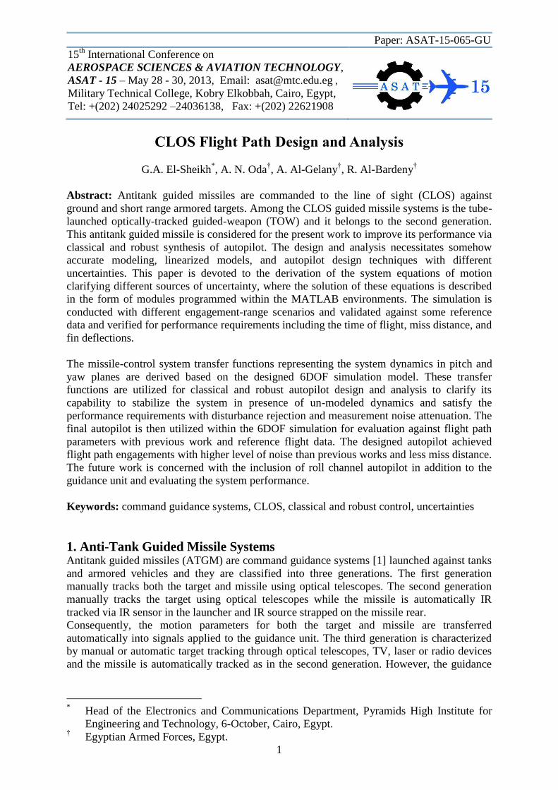
The simulation is conducted with nominal and perturbed values and depicted with the
reference as shown in Fig. 6. This Figure reveals that the established flight simulation which
had programmed within the MATLAB environments yield trajectories that are nearly
consistent with reference trajectories. The obtained results yield the appropriate and somehow
accurate model that can be used for the guidance and control design.

Paper: ASAT-15-065-GU
8
Fig. 5 Flowchart of the 6DOF flight simulation model
4. Autopilot Design and Analysis The ever-increasing development of tanks capabilities necessitates the design of accurate
control and guidance system for an antitank missile in presence of disturbance, measurement
noise, and un-modeled dynamics. To achieve this objective, the above sections of the paper
extracted a nonlinear mathematical model representing the dynamical behavior of the
underlying missile for different flight phases. The system uncertainties included thrust
variation due to different causes, variation in aerodynamic coefficients and parameters, wind
velocity in different directions and different trim conditions. To overcome different sources of
uncertainty, robust control is used to design the autopilot such that the system is stable with
the ability to overcome un-modeled dynamics, to reject the disturbances and minimize the
Paper: ASAT-15-065-GU
9
effects of measurement noises overall the missile flight envelope. The performance
specifications include overshoot, speed of response, steady state error, and system stability in
addition to flight paths with different engagement scenarios. To overcome the effects due to
uncertainties and achieve the performance requirements this section is devoted to design the
autopilot for the underlying command to line-of-sight (CLOS) system using the classical and
, -robust with evaluation. This control system is said to be robust when it maintains a
satisfactory level of stability and performance over a range of plant parameters, disturbances
and noises [7]. Thus, the objective is to investigate the robustness of the designed autopilot
against uncertainties due to different sources. The designed controller is implemented within
the missile control system and should be insensitive to model uncertainties and be able to
suppress disturbances and noise over the whole envelope of operation to prove its robustness.
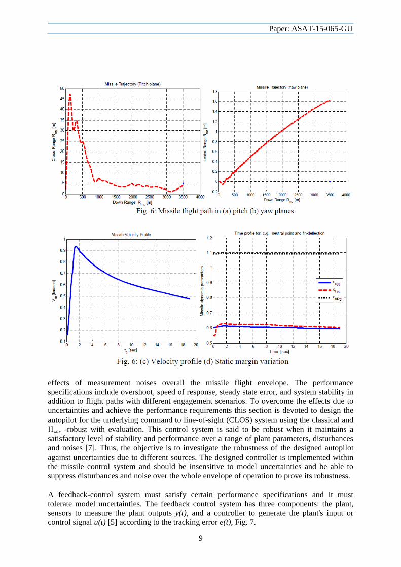
A feedback-control system must satisfy certain performance specifications and it must
tolerate model uncertainties. The feedback control system has three components: the plant,
sensors to measure the plant outputs y(t), and a controller to generate the plant's input or
control signal u(t) [5] according to the tracking error e(t), Fig. 7.
Paper: ASAT-15-065-GU
10
Fig. 7 Feedback Control
4.1 Pitch Airframe Dynamics Towards the autopilot design, the guidance equations have to be linearized for extracting the
necessary airframe transfer function or state space models that can be used for autopilot
design and analysis. That is, consider equations which describe equations of motion for the
intended guided missile, with the assumptions [4,6,9,15]: planer motion, constant velocity,
small firing angles ( , ). and zero thrust misalignment. The obtained linearized equations
describing dynamics of the guided missile c.g motion, rotation around c.g. and geometrical
relations can be summarized as follows:
Applying the Laplace transform and algebraic manipulation to Eq
ns 12 yield the obtained
airframe transfer functions as:
The pitch control system structure is shown in Fig. 8, where the gyro is a rate gyro used to
measure the body angular rate. The airframe transfer function ( ̇ ) expressed in Eqns
10 is
obtained via conducting the 6DOF simulation with target at distance 2500 [m] and
considering 10 operating points during the flight envelope. The extracted airframe transfer
function has the form ̇
.
Fig. 8 Pitch control system
Paper: ASAT-15-065-GU
11
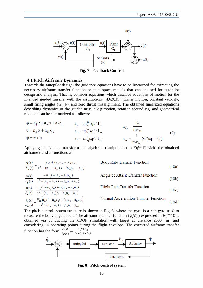
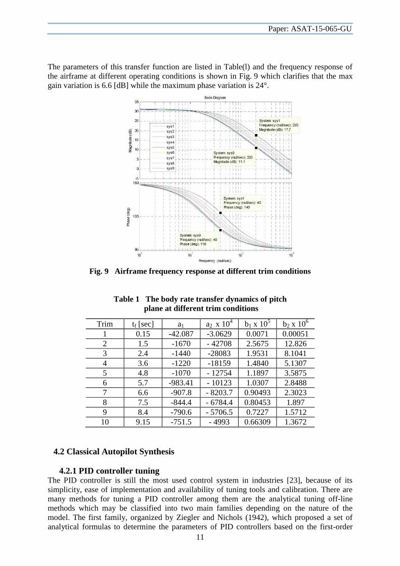
The parameters of this transfer function are listed in Table(l) and the frequency response of
the airframe at different operating conditions is shown in Fig. 9 which clarifies that the max
gain variation is 6.6 [dB] while the maximum phase variation is 24°.
Fig. 9 Airframe frequency response at different trim conditions
Table 1 The body rate transfer dynamics of pitch
plane at different trim conditions
Trim tf [sec] a1 a2 x 104
b1 x 105
b2 x 106
1 0.15 -42.087 -3.0629 0.0071 0.00051
2 1.5 -1670 - 42708 2.5675 12.826
3 2.4 -1440 -28083 1.9531 8.1041
4 3.6 -1220 -18159 1.4840 5.1307
5 4.8 -1070 - 12754 1.1897 3.5875
6 5.7 -983.41 - 10123 1.0307 2.8488
7 6.6 -907.8 - 8203.7 0.90493 2.3023
8 7.5 -844.4 - 6784.4 0.80453 1.897
9 8.4 -790.6 - 5706.5 0.7227 1.5712
10 9.15 -751.5 - 4993 0.66309 1.3672
4.2 Classical Autopilot Synthesis
4.2.1 PID controller tuning The PID controller is still the most used control system in industries [23], because of its
simplicity, ease of implementation and availability of tuning tools and calibration. There are
many methods for tuning a PID controller among them are the analytical tuning off-line
methods which may be classified into two main families depending on the nature of the
model. The first family, organized by Ziegler and Nichols (1942), which proposed a set of
analytical formulas to determine the parameters of PID controllers based on the first-order

Paper: ASAT-15-065-GU
12
plus dead time process model. This model is identified by step response (Ziegler-Nichols first
method) or by frequency response (Ziegler-Nichols second method). Because of its
simplicity, the Ziegler-Nichols method is still widely used despite the fact that they do not
address the robustness and the performance of the system. Automatic tuning of PID
parameters has also been proposed by Astrom and Hagghmd [ 2 , 3] that extended the Ziegler-
Nichols (first and second) methods to the automatic tuning of the PID controller. The auto-
tuning technique is obtained by combining the methods for determining the process dynamics
with the method for computing the PID parameters. The PID tuning methods are utilized with
the pitch transfer functions from which the selected controller parameters are listed in
Table (2).
Table 2 Classical controller parameters
Parameter PD PI PID
KP -326.332 -0.4859 -1.8357
KD -2.7974 — -0.048795
K, — -0.1288 -0.90368
Rise time [sec] 0.000526 0.087 0.0234
Settling time [sec] 0.00437 0.305 0.0758
O.S. [XI 10.4 9.38 9.05
Gain margin [dB] On OO OO
Phase margin [deg] 60 60.3 60
4.2.2 Controller performance evaluation
Step Response: Let us consider the 6th pitch airframe transfer function as a nominal airframe
which has a moderate frequency response compared with the remainder trim points. Using the
tuned classical controllers (PD, PI, PID) of Table (2), the step response for the pitch autopilot
is shown in Fig. 10, where the response parameters are given in Table (2). The results clarify
that the PD yields faster response with little increase in overshoot.
Noise Attenuation: Applying white Gaussian noise to the sensor output with noise to signal
ratio (NSR) 7%. the obtained control effort is shown m Fig. 11. winch clarify that PD
controller is more sensitive to additive noise compared to others.
Disturbance Rejection: An impulse disturbance is applied at the system output; according to
which they obtained step response of closed loop system is shown m Fig. 12. This figure
which clarifies that the convergence using PD after applying a disturbance is the best
compared to other controllers as it rejects 50% within 0.01 sec and reject 95% within 0.04sec.
The PI controller rejects 50% within 0.09 sec and reject 95% within 0.35sec while the PID
controller rejects 50% within 0.03sec and reject 95% within 0.15sec.
Unmodeled Dynamics: The three designed controllers are implemented at the different
operating points from which the obtained results clarify that the controller obtained taking the
6th
, 3th
and 9th
operating points as a nominal transfer function is not stable against all
unmodeled dynamics for the original autopilot while it is stable against all unmodeled
dynamics for the designed autopilot as shown in Fig. 13.

Paper: ASAT-15-065-GU
13
Fig. 10 Classical Pitch channel step
response
Fig. 11 Classical control effort with noise
4.2.3 Flight path analysis Guidance system evaluation represents one of the major tasks following the autopilot design.
This evaluation is carried out by conducting the 6DOF simulation using the autopilot with
different engagement scenarios. Some of these scenarios are shown in Fig. 14, which compare
between the systems with proportional and the obtained PD controllers. Applying the
proportional controller, the missile can hit the ground but with PD controller the missile hits
the target as shown in Fig. 15 by less miss-distance. On the other hand, the missile attack the
target but with large miss-distance using proportional controller while by applying the PD
controller this miss-distance is reduced to become very small. Applying the PI and PID
controller the miss-distance is very high which is not accepted and the system is not stable.
Fig. 12 Classical pitch disturbance
response
Fig. 13 Step response using PD
Paper: ASAT-15-065-GU
14
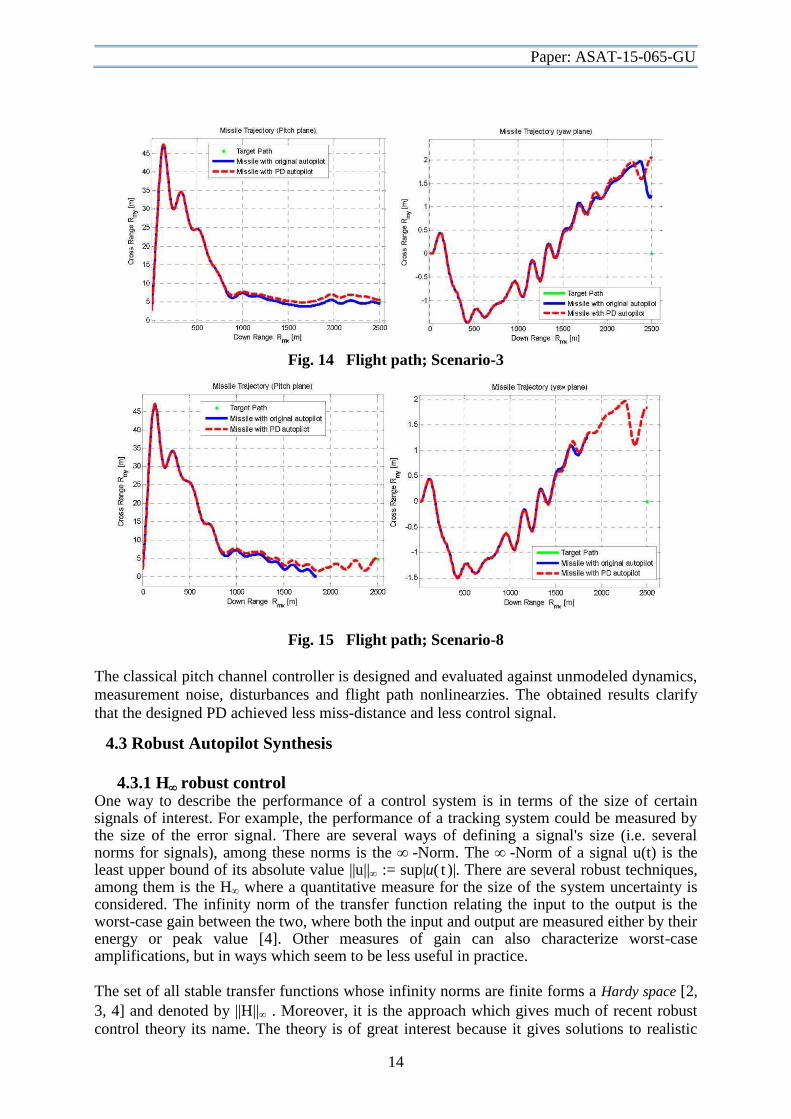
Fig. 14 Flight path; Scenario-3
Fig. 15 Flight path; Scenario-8
The classical pitch channel controller is designed and evaluated against unmodeled dynamics,
measurement noise, disturbances and flight path nonlinearzies. The obtained results clarify
that the designed PD achieved less miss-distance and less control signal.
4.3 Robust Autopilot Synthesis
4.3.1 H robust control One way to describe the performance of a control system is in terms of the size of certain signals of interest. For example, the performance of a tracking system could be measured by the size of the error signal. There are several ways of defining a signal's size (i.e. several norms for signals), among these norms is the -Norm. The -Norm of a signal u(t) is the least upper bound of its absolute value ||u|| := sup|u( t )|. There are several robust techniques, among them is the H where a quantitative measure for the size of the system uncertainty is considered. The infinity norm of the transfer function relating the input to the output is the worst-case gain between the two, where both the input and output are measured either by their energy or peak value [4]. Other measures of gain can also characterize worst-case amplifications, but in ways which seem to be less useful in practice. The set of all stable transfer functions whose infinity norms are finite forms a Hardy space [2,
3, 4] and denoted by ||H|| . Moreover, it is the approach which gives much of recent robust
control theory its name. The theory is of great interest because it gives solutions to realistic

Paper: ASAT-15-065-GU
15
robust control problems known as ||H|| optimization problems. The methods of H synthesis
are powerful tools for designing robust feedback control systems to achieve singular value
loop shaping specifications. The standard H control problem is sometimes also called the H
small gain problem. The small-gain theorem states that if a feedback loop consists of stable
systems, and the product of all their gains is smaller than one, then the feedback loop is stable
[1,7,19]. That is, assuming that the blocks P and C in Fig. 16 are stable, then the closed loop
system remains stable if 1 1
1y uT , where 1 1y uT is the feedback closed loop transfer
function. The small gain problem shows a general setup, and the problem of making
1 11y uT
is also called the small-gain problem. For H design problem, the state-space model
of an augmented plant P(s) with weighting functions W p ( s ) , Wu( s ) , and Wt( s ) which
penalize the error signal, control signal and output signal, respectively, is formulated as
shown in Fig. 17 so that the closed-loop transfer function matrix is the weighted mixed
sensitivity; 1 1
T
y u p u tT = W S W M W T . In practice, it is usually not necessary to obtain a
true optimal controller, but it is often simpler to find a sub-optimal controller. Suppose that
min is the minimum value of ,iF P C
over all possible stabilizing controllers C. Then, the
H sub-optimal control problem is: Given a > min, find all stabilizing controllers such that
,iF P C
< . This problem can be solved efficiently using the algorithm of Doyle et al.
(1989), by reducing iteratively to yield the optimal solution [5].
Fig. 16 Small Gain Problem
Fig. 17 Augmented Plant .P(s)
4.3.2 Robust autopilot design trials
A robust controller is designed using the following weights:
The obtained controllers are of high order that can be reduced using model-order reduction
techniques to yield the following;
Paper: ASAT-15-065-GU
16
The obtained results clarify that the multiplicative reduction method yield better result which
is consistent with the non reduced controller and consequently it will be used forward in this
work.
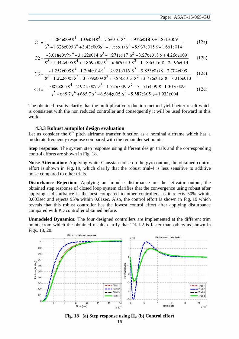
4.3.3 Robust autopilot design evaluation Let us consider the 6
th pitch airframe transfer function as a nominal airframe which has a
moderate frequency response compared with the remainder set points.
Step response: The system step response using different design trials and the corresponding
control efforts are shown in Fig. 18.
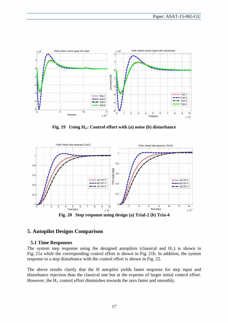
Noise Attenuation: Applying white Gaussian noise on the gyro output, the obtained control
effort is shown in Fig. 19, which clarify that the robust trial-4 is less sensitive to additive
noise compared to other trials.
Disturbance Rejection: Applying an impulse disturbance on the jetivator output, the
obtained step response of closed loop system clarifies that the convergence using robust after
applying a disturbance is the best compared to other controllers as it rejects 50% within
0.003sec and rejects 95% within 0.01sec. Also, the control effort is shown in Fig. 19 which
reveals that this robust controller has the lowest control effort after applying disturbance
compared with PD controller obtained before.
Unmodeled Dynamics: The four designed controllers are implemented at the different trim
points from which the obtained results clarify that Trial-2 is faster than others as shown in
Figs. 18, 20.
Fig. 18 (a) Step response using H (b) Control effort
Paper: ASAT-15-065-GU
17
Fig. 19 Using H: Control effort with (a) noise (b) disturbance
Fig. 20 Step response using design (a) Trial-2 (b) Tria-4
5. Autopilot Designs Comparison
5.1 Time Responses
The system step response using the designed autopilots (classical and H) is shown in
Fig. 21a while the corresponding control effort is shown in Fig. 21b. In addition, the system
response to a step disturbance with the control effort is shown in Fig. 22.
The above results clarify that the H autopilot yields faster response for step input and
disturbance rejection than the classical one but at the expense of larger initial control effort.
However, the H control effort diminishes towards the zero faster and smoothly.

Paper: ASAT-15-065-GU
18
Fig. 21 Response using PD and H (a) Step (b) Control effort
Fig. 22 Response using PD and H (a) Step disturbance (b) Control effort
5.2 Flight Path Evaluation The designed controllers are converted into differential equations inside the 6DOF model, the
simulation of which in conjunction with engagement parameters of Table (3) yield the flight
path trajectories shown in Figs. 23,24.
The obtained results reveal that the designed robust trial-4 has somehow slow step response
than trial-2 but it is less sensitive to the applied disturbance and noise and has a successful
flight path trajectory compared to the second trial. Table (3) shows a comparison between the
classical controller and the robust controllers via flight parameters.

Paper: ASAT-15-065-GU
19
Fig. 23 Flight Path Scenario-5
Table (3) Scenarios with comparison between PD and robust autopilots
Engagement
Scenario
Target Position Vtz NSR Thrust Miss-Distance
Rtk [tan] Rtv [m] [m/sec] [N] P PD Robust
1 2 5 0 0 1.06 1.5 1.33 1
*1 2 10 8 0 1 1.67 0.95 0.85
J 2.5 5 0 0 1 1.34 2 2
4 3.5 5 0 0 1 1.22 2.47 2.85
5 2 3 0 0.05 1 G. Impact 1.92 1.9
6 2.5 5 8 0.049 1 G. Impact 2.6 2.4
7 2.5 5 0 0.046 1 G. Impact 1.9 1.99
8 3.5 5 0 0 0.95 2.3 1.1 0.45

Paper: ASAT-15-065-GU
20
Fig. 24 Flight Path Scenario-8
6. Conclusion The paper presented the modeling of the intended system concerning the reference frames,
coordinates' transformations and equations of motion. This model is built in the form of
modules assigned to each process within the guided missile system. Then, it is programmed
within the MATLAB environments. The simulation is conducted with different engagement
scenarios and different sources of uncertainties including thrust variation, errors in
aerodynamic coefficients and wind velocity effects. The simulation results are validated
against reference data with different levels of uncertainty which clarify appropriateness of
built 6DOF model for autopilot and guidance laws design. This paper presented the derivation
of linearized equations from which the different aerodynamic transfer functions are extracted
and calculated at different engagement scenarios. The pitch channel controller is designed and
evaluated against unmodeled dynamics, measurement noise, disturbances and flight path
nonlinearzies. The obtained results clarify that the designed PD achieved less miss-distance
and less control signal. Then, the paper presented the robust H control theory with different
sensitivities and norms. In addition, it presented the model reduction techniques that can be
utilized for reducing the controller order and the appropriateness of multiplicative method.
The autopilots designed are evaluated against unmodeled dynamics, disturbance rejection,
noise attenuation and flight path. The obtained results clarify that the H controller is more
robust than the classical.
Paper: ASAT-15-065-GU
21
7. References Abd El-Latif, M.A., Robust Guidance and Control Algorithms in Presence of [1]
Uncertainties, MSc Thesis, Guidance Department. M.T.C., Cairo, Egypt, 2006.
Aly, M.S., Dynamical Analysis of Anti-Tank Missile Systems, Proceedings of the 9th [2]
int. AMME conference, 16-18 May, 2000.
Aly, M.S., Linear Model Evaluation of Command Guidance Systems. Proceedings of [3]
the 8th Int. conference on aerospace science and aviation technology, pp 1001-1003, 4-6
May, 1999.
Blakelock, J.B., Automatic Control of Aircraft and Missiles, Second Edition, John [4]
Wiley & Sons 1991.
El-Halwagy, Y.Z.. M.S. Aly, and M.S. Ghoniemy, Command Guidance System [5]
Simulation Airframe Analysis, Proceedings of the 7th Int. conference on aerospace
science and aviation technology, 13-15 May, 1997.
El-Sheikh, G.A., Guidance: Tlieon> and Systems, MTC, 2012. [6]
El-Sheikh, G.A., M.A. Abd-Altief and M.Y. Dogheish, Anti-Tank Guided Missile [7]
Performance Enhancement: Part-2: Robust Controller Design. 5th ICEENG Conference,
GC-10, MTC, Cairo, Egypt, May 16-18, 2006.
EL-Sheikh, G.A., M.J.Grimble, and M.A.Johanson, On the performance of GH^ Self-[8]
Timing for Aero Engine Control, control-97. Warwick University, March 01-07,1997,
pp 1306-1310.
Gamell P. and East D. J., Guided Weapon Control Systems. 2nd edition, Pergamon [9]
press, New York, 1980.
Hashad. A.I., An Enhancement System For Guidance and Control of IR Command [10]
Guided Missiles, M.Sc Thesis, Military Technical College, 1988.
Hertfordshire, S., Guided Weapons, British aircraft corporation, England, May, 1975. [11]
Locke S. and East D.J.. Principles of Guided Missile Design, Van Nostraud Reinhold [12]
company Inc., 1955.
Michael selig, Brian fucsz, Flight Simulation, May, 2003. [13]
Nasr Al-Hamwi, Robust Control and its Application to Antitank Guided Missile [14]
System. PhD Thesis. MTC Cairo. 2001.
Puckett. A.E., and S.Ramo. Guided Missile Engineering, McGraw Hill, 1959. [15]