cloud removal based on sparse representation via ... · cloud removal based on sparse...

2998 IEEE TRANSACTIONS ON GEOSCIENCE AND REMOTE SENSING, VOL. 54, NO. 5, MAY 2016

Cloud Removal Based on Sparse Representation viaMultitemporal Dictionary Learning

Meng Xu, Student Member, IEEE, Xiuping Jia, Senior Member, IEEE,Mark Pickering, Member, IEEE, and Antonio J. Plaza, Fellow, IEEE

Abstract—Cloud covers, which generally appear in optical re-mote sensing images, limit the use of collected images in manyapplications. It is known that removing these cloud effects is anecessary preprocessing step in remote sensing image analysis.In general, auxiliary images need to be used as the referenceimages to determine the true ground cover underneath cloud-contaminated areas. In this paper, a new cloud removal approach,which is called multitemporal dictionary learning (MDL), is pro-posed. Dictionaries of the cloudy areas (target data) and thecloud-free areas (reference data) are learned separately in thespectral domain. The removal process is conducted by combiningcoefficients from the reference image and the dictionary learnedfrom the target image. This method could well recover the datacontaminated by thin and thick clouds or cloud shadows. Ourexperimental results show that the MDL method is effective in re-moving clouds from both quantitative and qualitative viewpoints.

Index Terms—Cloud removal, dictionary learning, image recon-struction, multitemporal, sparse representation.

I. INTRODUCTION

W ITH the development of remote sensing technology,satellite images have become very useful in a variety

of applications, including the following: Earth observation, cli-mate change, and environmental monitoring. However, opticalremote sensing images are often contaminated by clouds andcloud shadows since optical sensors acquire data at the visibleand near-infrared wavelengths [1]. Cloud cover is consideredto be a severe problem in optical images because it also leadsto cloud shadow emerging. Both clouds and cloud shadowswill degrade the utilization of image data and limit the use ofthese optical remote sensing images in further applications. Forthis reason, the process of removing clouds is necessary forimproving the usefulness of optical remote sensing images.

Cloud effects vary due to their different compositions andheights. Opaque clouds obscure all the reflectance from theEarth’s surface, allowing no ground cover signal to be collected

Manuscript received July 6, 2015; revised October 27, 2015; acceptedDecember 10, 2015. Date of publication January 14, 2016; date of currentversion March 25, 2016.

M. Xu, X. Jia, and M. Pickering are with the School of Engineering andInformation Technology, University of New South Wales, Canberra, A.C.T.2600, Australia (e-mail: [email protected]; [email protected];[email protected]).

A. J. Plaza is with the Hyperspectral Computing Laboratory, Department ofTechnology of Computers and Communications, University of Extremadura,10003 Cáceres, Spain (e-mail: [email protected]).

Color versions of one or more of the figures in this paper are available onlineat http://ieeexplore.ieee.org.

Digital Object Identifier 10.1109/TGRS.2015.2509860

by sensors. In this paper, we particularly focus on the case ofthin clouds that do not entirely cover the signal correspondingto the underlying objects, as opposed to opaque clouds whichentirely dominate the pixel spectral signature. The task ofremoving clouds is treated as an image restoration problem.A number of cloud removal methods have been developed toaddress this problem. The related approaches can be classifiedinto two categories: individual-based and multitemporal-basedmethods.

In individual-based methods, cloud removal is implementedby making use of other bands from the individual image tomodel the cloud effects. An automatic thin cloud removalmethod utilizing the cirrus band as the auxiliary multispectraldata was proposed in [2]. The relationships between the cirrusband in Landsat 8 Operational Land Imager (OLI) and otherbands were used to model cloud effects. In [3], the hazeoptimized transformation method was proposed based on thehigh correlation between visible bands under clear atmosphericconditions and corrected for cloud effects by recovering howthe linear relationship deviated as a result of clouds. The authorin [4] used the near-infrared bands to estimate the spatialdistribution of haze in visible bands by building a linear modelover deep water regions. However, overcorrection will appearwhen clouds are not relatively thin. Generally, these individual-based cloud removal methods have difficulty mitigating theeffects of thick clouds.

In contrast, multitemporal-based methods are capable ofdealing with both thin and thick clouds. Since satellites re-visit the same geographical location periodically, multitempo-ral cloud-free images can be acquired for the same locationat different dates. A cloud removal method based on cloneinformation was developed in [5]. Data from multitemporalimages with no clouds were cloned to the cloudy patches basedon the Poisson equation and a global optimization process.A cloud removal method by applying image fusion and amultiscale wavelet-based approach was proposed in [6], usingtarget cloudy and multitemporal clear images to generate cloud-free images. Some methods designed for filling the gaps inLandsat ETM+Scan Line Corrector (SLC)-off imagery basedon this idea have been also applied to the cloud removal task[7], [8]. For instance, a modified neighborhood similar pixelinterpolator (MNSPI) cloud removal approach was proposedin [9] to predict the value of pixels blocked by thick cloudsfrom its neighboring similar pixels with the help of auxiliaryno-cloud images.

Cloud shadows are another problem which is even moredifficult to cope with. Cloud shadows occur when the cloud

0196-2892 © 2016 IEEE. Personal use is permitted, but republication/redistribution requires IEEE permission.See http://www.ieee.org/publications_standards/publications/rights/index.html for more information.

XU et al.: CLOUD REMOVAL BASED ON SPARSE REPRESENTATION VIA MULTITEMPORAL DICTIONARY LEARNING 2999

occludes the sunlight and prevents it from reaching the landsurface [10]. Therefore, the areas contaminated by cloud shad-ows have normally lower reflectance than other regions. Lu [11]developed a cloud/shadow detection and substitution methodbased on maximum and minimum filters. This method needsthresholds determined by trial and error to extract clouds orshadows. Hence, the method exhibits limited accuracy whenshadows cover high-reflectance surfaces or for thin clouds,which allow image regions to remain bright in these cases.In [12], a masking method was developed to detect cloudand cloud shadow in Landsat imagery over water and land,separately. Cloud shadow effects were detected by using a near-infrared band to set up a shadow layer.

Dictionary learning techniques are another option for cloudydata correction. Dictionary learning is a key component insparse representation theory which has received a growinginterest for the decomposition of signals into a subset of linearprojections from an overcomplete dictionary. Dictionary learn-ing methods aim at searching a data set to best represent thesignals by only using a small subset of the dictionary (i.e., afew atoms). Sparse representation has been employed in manyapplications, such as image denoising [13], face recognition[14], feature extraction and classification [15], and image su-perresolution [16]. With regard to cloud removal, a method wasproposed in [17] for the reconstruction of cloudy areas based oncompressive sensing theory. The basis pursuit and orthogonalmatching pursuit approaches were adopted for addressing thesparse representation. Genetic algorithms have been also ex-ploited to obtain the best solution of an �0-norm optimizationproblem. Most recently, a method has been developed in [18]using two multitemporal dictionary learning methods basedon the expanded K-SVD (K-means clustering process) andBayesian algorithms to recover quantitative remote sensingproducts contaminated by thick clouds and shadows. Thismethod sorts a set of time series data according to the temporalcorrelations for K-SVD and adjusts the weights in a Bayesianscheme. So far, cloud removal methods based on dictionarylearning are very limited and have been only employed in thespatial domain.

In this paper, a cloud removal method is developed bycombining multitemporal and dictionary learning methods.Specifically, we propose a new data restoration approach, whichis called multitemporal dictionary learning (MDL), based onsparse representation to remove cloud and cloud shadow ef-fects. Dictionaries of the cloudy areas (target data) and thecloud-free areas (reference data) are learned separately in thespectral domain, where each atom is associated with a groundcover component under the two aforementioned conditions.Meanwhile, cloud detection is not a required preprocessing stepin the proposed method. The cloud information is reflected inthe coefficients of the cloudy target image. The removal processis conducted by combining the coefficients from the referenceimage and the dictionary from the target image.

The remainder of this paper is organized as follows.Section II describes the proposed MDL method for recon-structing cloudy images. Section III gives an assessment of ourexperimental results. Finally, discussions and conclusions arepresented in Section IV.

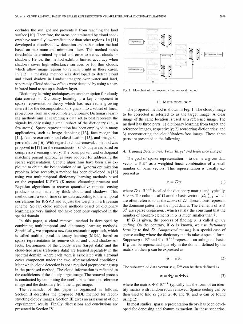
Fig. 1. Flowchart of the proposed cloud removal method.

II. METHODOLOGY

The proposed method is shown in Fig. 1. The cloudy imageto be corrected is referred to as the target image. A clearimage of the same location is used as a reference image. Themethod has three parts: 1) dictionary learning from target andreference images, respectively; 2) reordering dictionaries; and3) reconstructing the cloud/shadow-free image. These threeparts are presented in the following.

A. Training Dictionaries From Target and Reference Images

The goal of sparse representation is to define a given datavector x ∈ R

n as a weighted linear combination of a smallnumber of basis vectors. This representation is usually ex-pressed as

x = Dα (1)

where D ∈ Rn×k is called the dictionary matrix, and typically,

k > n. The columns of D are the basis vectors {di}ki=1, whichare often referred to as the atoms of D. These atoms representthe dominant patterns in the input data x. The elements of α ∈R

k are sparse coefficients, which satisfy the constraint that thenumber of nonzero elements in α is much smaller than k.

If D is given, the process of finding α is called sparsecoding. On the contrary, if α is known, we use dictionarylearning to find D. Compressed sensing is a special case ofsparse coding where the dictionary matrix takes a special form.Suppose y ∈ R

k and Ψ ∈ Rk×k represents an orthogonal basis.

If y can be represented sparsely in the domain defined by thematrix Ψ, then y can be expressed as

y = Ψα. (2)

The subsampled data vector x ∈ Rn can be then defined as

x = Φy = ΦΨα (3)

where the matrix Φ ∈ Rn×k typically has the form of an iden-

tity matrix with random rows removed. Sparse coding can bethen used to find α given x, Φ, and Ψ; and y can be foundusing (2).

In most studies, sparse representation theory has been devel-oped for denoising and feature extraction. In these scenarios,


Fig. 2. Illustration of dictionary learning in the spectral domain.

sparse representations of the data in the image domain havebeen exploited, with a sliding window of various sizes. Giventhat cloud and cloud shadow effects do not follow a distinctpattern within a spatial window, the cloud contaminations aredifferent for different pixels. On the other hand, the contamina-tion on each spectral band of a given pixel is highly related, i.e.,the true reflected spectrum from each pixel is modified whenthere is a cloud/shadow cover. Therefore, we propose to exploitsparse representations of the data in the spectral domain. Thewindow size is b× 1, where b is the number of spectral bands.A block diagram showing how the data are expressed, in ourmethod, by a sparse representation in the spectral domain, isshown in Fig. 2.

Let X = [x1, . . . ,xn] ∈ Rb×n represent a spectral image

signal with b bands and n = r × c pixels. Then, let xi satisfy

minD∈C,α∈Rb×n

n∑

i=1

1

2‖xi −Dαi‖22 s.t. D ≥ 0, ∀αi ≥ 0 (4)

where D ∈ Rb×k is the dictionary, and each column di is

a basis vector. Nonnegative constraints are enforced in thedecomposition process to make the values of α meaningful. Cis the convex set of matrices with the following constraint:

C �{D ∈ R

b×k s.t. ∀j=1, . . . , k, ‖dj‖2 ≤ 1 and dj ≥ 0}.

(5)

This is a joint optimization problem with respect to the dictio-nary D and the coefficients A = [α1, . . . ,αn] ∈ R

k×n. Thisjoint minimization problem is not convex. However, a convexminimization problem can be formulated with respect to eachof D and A if the other is fixed. The online dictionary learningmethod proposed in [19] takes this approach, and we proposeto use this method to solve the joint optimization problemdescribed earlier.

The online dictionary learning method can be summarizedas follows. The initial dictionary D0 is provided with randomelements from a training set. Sparse coding steps are used to

compute the coefficients A using the Least Angle Regression(LARS) method [20]. Then, the updated dictionary Dt is foundby minimizing

Dt � argminD∈C

1

n

n∑

i=1

1

2‖xi −Dαi‖22 (6)

using a block-coordinate descent approach with respect to thejth column dj while keeping the other columns fixed with theconstraint ‖dj‖2 ≤ 1. This process is then repeated usingthe updated dictionary until a convergence criterion is satis-fied (for a more detailed explanation of the online dictionarylearning method, please refer to [19]).

This spectral domain sparse representation approach is ap-plied to the problem of cloud and cloud shadow removal inthe following manner. Let Xt ∈ R

b×n be the target imagecontaminated by clouds andXr ∈ R

b×n be the reference imageof the same geographical region from a clear day. Let n = r × cbe the total number of pixels of an image of r rows byc columns, and b is the number of spectral bands. The columnsof Xt and Xr correspond to the spectral vectors of each pixel.k is the number of columns in the dictionary. Let Dt and Dr

denote the dictionaries of the target and reference images,respectively. Then, the sparse representation of the target andreference images can be expressed as

Xt = DtAt + εt (7)Xr = DrAr + εr. (8)

Dictionaries Dt and Dr are learned separately using the onlinedictionary learning method introduced earlier.

In general, dictionaries are an overcomplete matrix and canreflect the basic patterns contained in each window. In our case,the dictionaries represent the spectra of fundamental compo-nents which all the pixels contain, and the sparse coefficientsare the weights of the associated components. In other words,each measured pixel spectrum is a weighted sum of the spectraof a few selected fundamental components (atoms).

B. Dictionary Reordering

When there is a cloud cover, we can expect that the fun-damental components that a pixel contains remain unchanged.Therefore, the same number of atoms for the two dictionariesis selected. However, the two dictionaries are not identicaldue to two reasons. First, the order of the atoms may notbe the same since they are generated separately during eachdictionary training. Second, the atoms corresponding to thesame spectral components (subclasses) change with imagingconditions. Nevertheless, the corresponding atoms from thecloudy/shadowy image should have the same pattern as thosefrom the clear image and are highly correlated. It is importantthat the two dictionaries are in the same order for performingthe next step of the proposed method. Hence, reordering isperformed using the correlation matrix (CM) between the atomsin the two dictionaries. The CM is determined by calculating thecorrelation coefficient (CC) between each atom in Dt and Dr.Every element in the CM is the CC of the two dictionaries. Asa result, the CM is a k × k matrix in which the nth column


represents the CC of the nth atom in Dt with all the atomsin Dr. The reordered matrix is generated by searching thehighest CC value of each column in the CM. Each column isreordered by moving the highest CC value to the nth row in thenth column. Then, each column in Dt will change according tothe movement in the CM. These steps are used to make sure thatthe two dictionaries have the same order. The new reordereddictionary is denoted by D∗

t.It has been observed that both dictionaries are composed of

the spectral vectors of various fundamental components of landcover materials. There is no cloud component in the dictionarywhich is learned from the cloudy image (target image), asillustrated in the experimental section. This result indicates thatthe dictionary is not affected by the cloud cover. This is animportant property and leads to the proposed method for cloudyimage restoration.

C. Cloudy Image Restoration

Based on the concept of sparse representation, we know thatAr determines which atoms are associated with a given pixeland what the corresponding weights are. This association willnot be changed due to cloud cover. However, the magnitudesof the atoms may be different and are affected by the differentimaging conditions, such as the changes in atmospheric param-eters. Therefore, to recover the signals for the target image, wepropose to use the (reordered) target image’s dictionary D∗

t andthe reference image’s coefficients Ar to reconstruct the clearimage. Specifically, the clear image is obtained as follows:

Xct = D∗

tAr (9)

where Xct is the reconstructed image after removing cloud and

cloud shadows.Our newly proposed MDL method can be applied to various

types of remote sensing data, including multispectral and hyper-spectral images. The only parameter that needs to be adjustedis the size of the dictionary k. Differing from conventionalcloud/shadow removal approaches, the proposed method canbe conducted without screening clouds or cloud shadows as apreprocessing step. Moreover, it is not affected by the size of thecloud/shadow cover area and the complexity of the background.

III. EXPERIMENTS AND RESULTS

A. Experiments on a Simulated Image

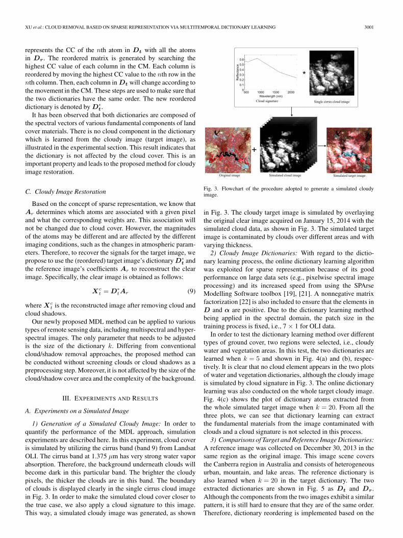
1) Generation of a Simulated Cloudy Image: In order toquantify the performance of the MDL approach, simulationexperiments are described here. In this experiment, cloud coveris simulated by utilizing the cirrus band (band 9) from LandsatOLI. The cirrus band at 1.375 μm has very strong water vaporabsorption. Therefore, the background underneath clouds willbecome dark in this particular band. The brighter the cloudypixels, the thicker the clouds are in this band. The boundaryof clouds is displayed clearly in the single cirrus cloud imagein Fig. 3. In order to make the simulated cloud cover closer tothe true case, we also apply a cloud signature to this image.This way, a simulated cloudy image was generated, as shown

Fig. 3. Flowchart of the procedure adopted to generate a simulated cloudyimage.

in Fig. 3. The cloudy target image is simulated by overlayingthe original clear image acquired on January 15, 2014 with thesimulated cloud data, as shown in Fig. 3. The simulated targetimage is contaminated by clouds over different areas and withvarying thickness.

2) Cloudy Image Dictionaries: With regard to the dictio-nary learning process, the online dictionary learning algorithmwas exploited for sparse representation because of its goodperformance on large data sets (e.g., pixelwise spectral imageprocessing) and its increased speed from using the SPArseModelling Software toolbox [19], [21]. A nonnegative matrixfactorization [22] is also included to ensure that the elements inD and α are positive. Due to the dictionary learning methodbeing applied in the spectral domain, the patch size in thetraining process is fixed, i.e., 7 × 1 for OLI data.

In order to test the dictionary learning method over differenttypes of ground cover, two regions were selected, i.e., cloudywater and vegetation areas. In this test, the two dictionaries arelearned when k = 5 and shown in Fig. 4(a) and (b), respec-tively. It is clear that no cloud element appears in the two plotsof water and vegetation dictionaries, although the cloudy imageis simulated by cloud signature in Fig. 3. The online dictionarylearning was also conducted on the whole target cloudy image.Fig. 4(c) shows the plot of dictionary atoms extracted fromthe whole simulated target image when k = 20. From all thethree plots, we can see that dictionary learning can extractthe fundamental materials from the image contaminated withclouds and a cloud signature is not selected in this process.

3) Comparisons of Target and Reference Image Dictionaries:A reference image was collected on December 30, 2013 in thesame region as the original image. This image scene coversthe Canberra region in Australia and consists of heterogeneousurban, mountain, and lake areas. The reference dictionary isalso learned when k = 20 in the target dictionary. The twoextracted dictionaries are shown in Fig. 5 as Dt and Dr.Although the components from the two images exhibit a similarpattern, it is still hard to ensure that they are of the same order.Therefore, dictionary reordering is implemented based on the


Fig. 4. Illustration of dictionary learning on the simulated target image. The original image was acquired on January 15, 2014.

Fig. 5. Illustration of the reordering procedure on the target dictionary according to the dictionary of the reference image.

proposed method. The CM is first calculated to present thecorrelation coefficients between each column in Dt and Dr .The purpose of reordering is to make the atom in Dt have thehighest correlation with the corresponding atom in Dr. Thereordered dictionary D∗

t is adjusted this way. The CM afterreordering is shown in Fig. 5 as well. There is little differencebetween the two matrices, and it should be noted that thecorrelation coefficients of each of the corresponding elementsare reasonably high before reordering. The mean value of the

correlation coefficients for each corresponding element in thetarget and reference dictionaries increased from 0.87 to 0.92after reordering. Therefore, we can conclude that the reorderingprocedure is a necessary process to make sure that the sparsecoefficients represent the associated components as accuratelyas possible.

4) Cloud Removal Results: To draw comparisons, theMNSPI method [9] was also applied to the simulated imagein our experiments. Mean absolute percentage error (MAPE),


Fig. 6. Landsat 8 OLI images used in the simulation experiments, withfalse color composite R = band 5, G = band 4, B = band 3. (a) Simulatedtarget cloudy image. (b) Reference image acquired on December 30, 2013.(c) Recovered image using the MNSPI method. (d) Recovered image using theproposed MDL method.

TABLE IQUANTITATIVE RESULTS OF SIMULATION EXPERIMENTS

USING THE PROPOSED MDL AND MNSPI METHODS

peak signal-to-noise ratio (PSNR), and CC were used to as-sess the proposed method quantitatively. The recovered imagesusing MNSPI and the proposed MDL method are shown inFig. 6(c) and (d), respectively. The MAPE, PSNR, and CC in-dexes of the simulated cloudy image and the images recoveredby MNSPI and MDL versus the original clear image are shownin Table I. The MAPE is defined as (1/N)

∑ni=1 |(xo(i)−

xc(i))/xo(i)|, where N is the total number of pixels conta-minated by clouds, and xo(i) and xc(i) are the original andrecovered image values, respectively. Three bands are evaluatedin Table I. The recovered image using the MDL method hasthe lowest MAPE value, which means that it is closest to theoriginal true data. The simulated cloudy image has a very lowPSNR value (10.74 dB, 10.51 dB, 14.42 dB), indicating that thesimulated clouds strongly affect the quality of the image. TheCCs for MDL improve more than for the MNSPI method inall three bands. The MNSPI method is effective in recovering

the edges of regions, but is sensitive to the size of the clouds.The large patches of simulated clouds decrease the accuracyof recovery by MNSPI. From the simulation experiments, wecan conclude that the proposed MDL method provides moreaccurate restoration results.

B. Experiments on Real Images

1) Cloud Removal for a Hyperion Image: In order to bettersubstantiate our restoration results, we also performed exper-iments on real hyperspectral data. One data set consisting ofEO-1 Hyperion images was tested. Two Hyperion images ac-quired on March 22, 2003 and March 6, 2003 were selected astarget and reference images, respectively. The target image iscontaminated by clouds and cloud shadows over large areas ofthe image. Fig. 7 illustrates the details of the recovery processusing the proposed MDL method on EO-1 data. The firstcolumn shows the target, reference, and recovered Hyperionimages with composite colors of R: band 49 (0.844 μm),G: band 45 (0.803 μm), and B: band 10 (0.447 μm). Thedictionaries and coefficients extracted from the target and ref-erence images, respectively, are shown in the second column inFig. 7. The number of elements in the dictionary is 20. Therecovered image was generated by combining the reorderedtarget image dictionaryD∗

t and the reference image coefficientsAr. A cloudy pixel, which is labeled by the red X, was selectedas an illustrative example. The spectral profiles of this pixel inthe target, reference, and recovered images are shown in thethird column. Each legend shows the coefficients correspondingto each extracted atom (spectra) in the dictionary. The markedpixel is generated by the sum of these values. Spectral profilesof the labeled pixel show that the MDL method can restorethe signatures of the ground covered by clouds. The differencebetween the reference and recovered spectra is regarded as thedifference in atmospheric conditions for the two dates. Thecloud shadow regions are also recovered in the results.

2) Cloud Removal for an OLI Image: Here, one real dataset from Landsat 8 OLI data is investigated using the proposedMDL method. The experimental OLI images were downloadedfrom the National Aeronautics and Space Administration web-site (http://earthexplorer.usgs.gov/). The OLI is a 30-m spatialresolution optical sensor with a 16-day revisit time. Therefore,it is possible to acquire time series data in the same geo-graphical area. The experimental target image was acquired onDecember 4, 2013, and the reference image was acquired onSeptember 18, 2013. These images contain 500 × 500 pixelswith seven spectral bands.

In Fig. 8, the target image is contaminated by relatively thinclouds over almost the entire image. The recovered image, asshown in Fig. 8(c), is visually clear and close to the referenceimage acquired on September 18. The number of dictionaryatoms is 30 in this experiment. The homogeneous and hetero-geneous areas are both corrected. In the top right corner ofthe scene, the urban area is restored well. Fig. 8(e)–(f) showszoomed images revealing clear edges and high quality. Theresults indicate that the proposed MDL method can recover dataaffected by different types of clouds and is not sensitive to thetype of ground covers.


Fig. 7. Details of cloud removal results for EO-1 Hyperion data. The target and reference images were acquired on March 22, 2003 and March 6, 2003,respectively.

IV. DISCUSSION AND CONCLUSIONS

In this paper, a cloud removal method, which is called MDLmethod, has been proposed. A reference image is required asauxiliary data for determining the fundamental componentsin each pixel contaminated by clouds. The dictionary learnedfrom the target image is reordered to match the atoms in thereference image. The recovery process is conducted by combin-ing the reordered target dictionary and the sparse coefficientsfrom the reference image. Simulated and real data were both

quantitatively and qualitatively investigated in our experiments.The recovery results show better performance of the proposedMDL method when compared with the MNSPI method. Ourproposed method can handle thin and thick clouds, as well ascloud shadows. The size of the contaminated areas is not alimitation for the proposed method. It should be noted that theonly parameter that needs to be set manually in the recoveryprocedure is the number of atoms in the dictionary. In theexperiments, various values for this parameter were tested to


Fig. 8. Cloud removal results for the Landsat 8 OLI images in real data exper-iments. (a) Target image acquired on December 4, 2013. (b) Reference imageacquired on September 18, 2013. (c) Recovered image using the proposed MDLmethod. (d)–(f) Zoomed images of the square area marked in (a)–(c).

obtain the best restoration results. This testing process indicatedthat the optimal value of this parameter varies for differentimage scenes. In the future, the reasons for this variation willbe investigated. Further applications of the MDL method willbe also explored.

ACKNOWLEDGMENT

The authors would like to thank the Editors and the anony-mous reviewers for their outstanding comments and sugges-tions, which greatly helped them to improve the technicalquality and presentation of this paper.

REFERENCES

[1] J. Ju and D. P. Roy, “The availability of cloud-free Landsat ETM+ dataover the conterminous United States and globally,” Remote Sens. Environ.,vol. 112, no. 3, pp. 1196–1211, Mar. 2008.

[2] M. Xu, X. Jia, and M. Pickering, “Automatic cloud removal for Landsat 8OLI images using cirrus band,” in Proc. IEEE IGARSS, 2014,pp. 2511–2514.

[3] Y. Zhang, B. Guindon, and J. Cihlar, “An image transform to character-ize and compensate for spatial variations in thin cloud contamination ofLandsat images,” Remote Sens. Environ., vol. 82, no. 2/3, pp. 173–187,Oct. 2002.

[4] C. Ji, “Haze reduction from the visible bands of Landsat TM and ETM+images over a shallow water reef environment,” Remote Sens. Environ.,vol. 112, no. 4, pp. 1773–1783, Apr. 2008.

[5] C.-H. Lin, P.-H. Tsai, K.-H. Lai, and J.-Y. Chen, “Cloud removal frommultitemporal satellite images using information cloning,” IEEE Trans.Geosci. Remote Sens., vol. 51, no. 1, pp. 232–241, Jan. 2013.

[6] D.-C. Tseng, H.-T. Tseng, and C.-L. Chien, “Automatic cloud removalfrom multi-temporal SPOT images,” Appl. Math. Comput., vol. 205,no. 2, pp. 584–600, Nov. 2008.

[7] J. Chen, X. Zhu, J. E. Vogelmann, F. Gao, and S. Jin, “A simple andeffective method for filling gaps in Landsat ETM+ SLC-off images,”Remote Sens. Environ., vol. 115, no. 4, pp. 1053–1064, Apr. 2011.

[8] X. Zhu, D. Liu, and J. Chen, “A new geostatistical approach for fillinggaps in Landsat ETM+ SLC-off images,” Remote Sens. Environ.,vol. 124, pp. 49–60, Sep. 2012.

[9] X. Zhu, F. Gao, D. Liu, and J. Chen, “A modified neighborhood similarpixel interpolator approach for removing thick clouds in Landsat images,”IEEE Geosci. Remote Sens. Lett., vol. 9, no. 3, pp. 521–525, May 2012.

[10] A. Shahtahmassebi, N. Yang, K. Wang, N. Moore, and Z. Shen, “Reviewof shadow detection and de-shadowing methods in remote sensing,” Chin.Geogr. Sci., vol. 23, no. 4, pp. 403–420, Aug. 2013.

[11] D. Lu, “Detection and substitution of clouds/hazes and their cast shadowson ikonos images,” Int. J. Remote Sens., vol. 28, no. 18, pp. 4027–4035,Sep. 2007.

[12] Z. Zhu and C. E. Woodcock, “Object-based cloud and cloud shadow de-tection in Landsat imagery,” Remote Sens. Environ., vol. 118, pp. 83–94,Mar. 2012.

[13] M. Elad and M. Aharon, “Image denoising via sparse and redundantrepresentations over learned dictionaries,” IEEE Trans. Image Process.,vol. 15, no. 12, pp. 3736–3745, Dec. 2006.

[14] J. Wright, A. Y. Yang, A. Ganesh, S. S. Sastry, and Y. Ma, “Robust facerecognition via sparse representation,” IEEE Trans. Pattern Anal. Mach.Intell., vol. 31, no. 2, pp. 210–227, Feb. 2009.

[15] Y. Chen, N. M. Nasrabadi, and T. D. Tran, “Hyperspectral image classifi-cation using dictionary-based sparse representation,” IEEE Trans. Geosci.Remote Sens., vol. 49, no. 10, pp. 3973–3985, Oct. 2011.

[16] J. Yang, Z. Wang, Z. Lin, S. Cohen, and T. Huang, “Coupled dictionarytraining for image super-resolution,” IEEE Trans. Image Process., vol. 21,no. 8, pp. 3467–3478, Aug. 2012.

[17] L. Lorenzi, F. Melgani, and G. Mercier, “Missing-area reconstructionin multispectral images under a compressive sensing perspective,” IEEETrans. Geosci. Remote Sens., vol. 51, no. 7, pp. 3998–4008, Jul. 2013.

[18] X. Li et al., “Recovering quantitative remote sensing products contami-nated by thick clouds and shadows using multitemporal dictionary learn-ing,” IEEE Trans. Geosci. Remote Sens., vol. 52, no. 11, pp. 7086–7098,Nov. 2014.

[19] J. Mairal, F. Bach, J. Ponce, and G. Sapiro, “Online learning for matrixfactorization and sparse coding,” J. Mach. Learn. Res., vol. 11, pp. 19–60,2010.

[20] B. Efron, T. Hastie, I. Johnstone, and R. Tibshirani, “Least angle regres-sion,” Ann. Stat., vol. 32, no. 2, pp. 407–499, Apr. 2004.

[21] J. Mairal, F. Bach, J. Ponce, and G. Sapiro, “Online dictionary learningfor sparse coding,” in Proc. 26th Annu. Int. Conf. Mach. Learn., 2009,pp. 689–696.

[22] D. D. Lee and H. S. Seung, “Algorithms for non-negative matrix factor-ization,” in Proc. Adv. Neural Inf. Process. Syst., 2001, pp. 556–562.

Meng Xu (S’13) received the B.S. and M.S. degreesin electrical engineering from Ocean University ofChina, Qingdao, China, in 2011 and 2013, respec-tively. She is currently working toward the Ph.D.degree in the School of Engineering and Informa-tion Technology, University of New South Wales,Canberra, Australia.

Her research interests include cloud removal andremote sensing image processing.

Xiuping Jia (M’93–SM’03) received the B.Eng. de-gree from Beijing University of Posts and Telecom-munications, Beijing, China, in 1982 and the Ph.D.degree in electrical engineering from the Universityof New South Wales, Canberra, Australia, in 1996.

Since 1988, she has been with the School of Infor-mation Technology and Electrical Engineering, Uni-versity of New South Wales, where she is currentlya Senior Lecturer. She is also a Guest Professor withHarbin Engineering University, Harbin, China, andan Adjunct Researcher with the National Engineer-

ing Research Center for Information Technology in Agriculture, Beijing. Shehas coauthored the remote sensing textbook Remote Sensing Digital ImageAnalysis [Springer-Verlag, 3rd (1999) and 4th eds. (2006)]. Her research in-terests include remote sensing, imaging spectrometry, and spatial data analysis.

Dr. Jia is an Editor of the Annals of GIS and an Associate Editor of the IEEETRANSACTIONS ON GEOSCIENCE AND REMOTE SENSING.


Mark Pickering (S’92–M’95) was born in Biloela,Australia, in 1966. He received the B.Eng. degreefrom the Capricornia Institute of Advanced Educa-tion, Rockhampton, Australia, in 1988, and theM.Eng. and Ph.D. degrees from the University ofNew South Wales, Canberra, Australia, in 1991 and1995, respectively, all in electrical engineering.

He was a Lecturer from 1996 to 1999 and aSenior Lecturer from 2000 to 2009 with the Schoolof Electrical Engineering and Information Technol-ogy, University of New South Wales, where he is

currently an Associate Professor. His research interests include video andaudio coding, medical imaging, data compression, information security, datanetworks, and error-resilient data transmission.

Antonio J. Plaza (M’05–SM’07–F’15) receivedthe Bachelor’s, M.Sc., and Ph.D. degrees from theUniversity of Extremadura, Extremadura, Spain, in1997, 1999, and 2002, respectively, all in computerengineering.

He is currently an Associate Professor (with ac-creditation for Full Professor) with the Departmentof Technology of Computers and Communications,University of Extremadura, where he is the Headof the Hyperspectral Computing Laboratory. From2007 to 2011, he was the Coordinator of the Hyper-

spectral ImagingNetwork, a European project with a total funding of 2.8 millioneuros. He has authored over 400 publications, including 126 JCR journal papers(78 in IEEE journals), 20 book chapters, and over 240 peer-reviewed conferenceproceeding papers (94 in IEEE conferences). He has edited the book High-Performance Computing in Remote Sensing (CRC Press/Taylor and Francis)(the first book on this topic in the published literature) and guest edited eightspecial issues on hyperspectral remote sensing for different journals.

Dr. Plaza served as the Chair for the 2011 IEEE Workshop on HyperspectralImage and Signal Processing: Evolution in Remote Sensing and the Directorof Education Activities for the IEEE Geoscience and Remote Sensing Society(GRSS) from 2011 to 2012. He has been serving as the President of the SpanishChapter of IEEE GRSS since November 2012. He served as an Associate Editorfor the IEEE TRANSACTIONS ON GEOSCIENCE AND REMOTE SENSING

from 2007 to 2012. He was a member of the Editorial Board of the IEEEGeoscience and Remote Sensing Newsletter from 2011 to 2012 and a memberof the steering committee of the IEEE JOURNAL OF SELECTED TOPICS IN

APPLIED EARTH OBSERVATIONS AND REMOTE SENSING in 2012. He is aGuest Editor of seven special issues on JCR journals (three in IEEE journals).He is also an Associate Editor of IEEE ACCESS and the IEEE GEOSCIENCE

AND REMOTE SENSING MAGAZINE. He has been serving as the Editor-in-Chief of the IEEE TRANSACTIONS ON GEOSCIENCE AND REMOTE SENSING

since January 2013. He was recipient of the Best Reviewers of the IEEEGeoscience and Remote Sensing Letters in 2009 and of the Best Reviewers ofthe IEEE TRANSACTIONS ON GEOSCIENCE AND REMOTE SENSING in 2010.

cloud removal based on sparse representation via ... · cloud removal based on sparse...

Documents