Club Good Intermediaries∗

Simon Loertscher† Leslie M. Marx‡

September 4, 2016

Abstract

The emergence and ubiquitous presence in everyday life of digital goods such

as songs, movies, and e-books give renewed salience to the problem of providing

public goods with exclusion. Because digital goods are typically traded via inter-

mediaries like iTunes, Amazon, and Netflix, the question arises as to the optimal

pricing mechanism for such club good intermediaries. We derive the direct Bayesian

optimal mechanism for allocating club goods when the mechanism designer is an

intermediary that neither produces nor consumes the goods, and we develop an

indirect mechanism that implements this mechanism. We also derive sufficient con-

ditions for the intermediary-optimal mechanism to be implementable with revenue

sharing contracts, which are widely used in e-business.

Keywords: revenue maximization, excludable public goods, two-sided platforms, optimal

pricing, digital goods

JEL Classification: C72, D82, L13

∗We thank seminar participants at the 34th Australasian Economic Theory Workshop, Cedric Wasser,and an anonymous referee for helpful comments.

†Department of Economics, Level 4, FBE Building, 111 Barry Street, University of Melbourne, Victoria3010, Australia. Email: simonl@unimelb.edu.au.

‡The Fuqua School of Business, Duke University, 100 Fuqua Drive, Durham, NC 27708, USA: Email:marx@duke.edu.

1 Introduction

The issue of optimal public goods provision has achieved new salience with the emergence

of digital goods like e-books, downloadable songs, and movies along with new technologies

that make exclusion and distribution possible at negligible marginal costs. An aspect not

present in the analysis of excludable public goods or “club goods” in the age of the

internet is that consumers gain access to these digital goods via an intermediary such as

Amazon, iTunes, Spotify, or Netflix rather than contracting directly with the producer

of the club good as they might with the owner of a country club. In this paper, we

provide an analysis of optimal mechanisms for club good intermediaries, which are brokers

who intermediate between the producer of a public good with exclusion and consumers.

Besides the aforementioned intermediaries for digital goods, crowdfunding platforms like

Kickstarter or Indiegogo are other examples of club good intermediaries.1

We analyze club good intermediaries within the independent private values paradigm

in Bayesian mechanism design, assuming that all agents draw their values and costs inde-

pendently from some commonly known distributions and that they are privately informed

about the realizations of their types. Among other things, the Bayesian mechanism design

approach has the benefit of imposing no constraints on the optimal mechanism other than

the usual incentive compatibility and individual rationality constraints.

We extend the methods and insights developed by Myerson (1981) and Myerson and

Satterthwaite (1983) for private goods to the case of club goods.2 Just as with a broker

for private goods, the optimal mechanism for a club good intermediary can be stated

in terms of virtual valuations and virtual costs, with trade occurring when the former

exceed the latter. However, the conditions for trade for a club good intermediary are

more intricate because the optimal allocation rule is such that trade occurs if and only if

the sum of the virtual values of those buyers with nonnegative virtual values exceeds the

seller’s virtual (fixed) cost for producing the good.3 Also, in the private good setting, the

mechanism need only determine a single price to be paid by the winning buyer. But in

the club good setting, the mechanism must determine a price for each buyer who receives

1For more on crowdfunding platforms, see, for example, Marwell (2015).2It is well known that under seemingly weak conditions (a lower bound support of the buyers’ type

distributions of zero) the Bayesian optimal mechanism allocates the public good with probability zeroin the large economy (Rob, 1989). With n buyers, the sum of the virtual types of the buyers convergesto n times the expected virtual type, which is equal to the lower bound of support of the buyers’ typedistribution, and hence to n times zero under the condition just stated. This provides further motivationto study Bayesian optimal provision of club goods.

3Bearing in mind the applications of digital goods, we assume that the marginal cost of deliveringevery additional copy is zero once the fixed cost of producing the good has been borne. In general,the constraint is that the sum of the virtual values of those buyers with virtual values no less than themarginal costs exceeds the seller’s virtual fixed cost.

1

the good, and these prices may differ across buyers as a function of the buyers’ reported

types and identities.

Besides characterizing the Bayesian optimal club good mechanism for an intermediary,

we define a club good clock auction in which it is a dominant strategy for buyers to exit at

their values. We provide generalizations that allow for congestion effects, nonmonotonic

virtual types that require ironing, and an objective for the designer that includes weight

on both profit and social surplus. We also derive sufficient conditions for the intermediary-

optimal mechanism to be implementable with revenue sharing contracts. These are widely

used in e-business and featured prominently in Apple’s e-book case.4

In some settings, whether a good is offered as a private good or as a public good

is a choice variable of the designer. For example, whether radio spectrum is used as a

public good with exclusion or under rivalry of consumption as a private good depends on

the technological standards, which may be a choice variable of the designer. Similarly,

artists can choose between selling private goods in the form of paintings and club goods

in the form of photographs. Under the assumptions that the demand and fixed cost

of production for the two kinds of goods are the same, our analysis shows that a profit

maximizing designer will choose to offer the good as a club good. In this way, our analysis

provides a way of endogenizing the choice of technological format for applications like

these.

First and foremost, our paper contributes to the large and growing literature on market

making and intermediation by introducing club goods. Thus far, this literature has either

focused on private goods – see, for example, Rubinstein and Wolinsky (1987), Stahl

(1988), Gehrig (1993), Spulber (1996), Rust and Hall (2003), Loertscher (2007, 2008),

or Loertscher and Niedermayer (2015) – or the need of market making intermediaries to

bring both sides on board, accounting for direct network effects, like Caillaud and Jullien

(2001, 2003), Rochet and Tirole (2002, 2006), or Gomes (2014). With club goods, there is

an indirect network even after both sides are on board because each buyer benefits from

additional buyers because they are a source of revenue and therefore make the provision

of the good more likely even though no buyer directly cares about any other buyer.5

Our paper is also related to the literature on the provision of excludable public goods.

Perhaps the paper closest to ours in this strand of literature is Schmitz (1997). Schmitz

studies a setup with one-sided private information and derives the optimal allocation

for a club good (allowing for congestion effects) for a profit maximizing seller under the

4“Ruling That Apple Led E-Book Pricing Conspiracy Is Upheld,” New York Times, June 30, 2015.5As discussed in Marwell (2015), this effect also arises in all-or-nothing fundraising models, where

fundraisers only collect donations if the total amount pledged exceeds a target and donors care about theamount raised. In concurrent work, Strausz (2015) analyzes the principal-agent problems that arise incrowdfunding. His work is complementary to ours, as we analyze the platform’s optimal pricing problemabsent moral hazard.

2

assumption of regularity. He shows that in the limit as the number of buyers goes to

infinity (and the cost increases with the number of buyers as in Rob (1989)), the profit

maximizing mechanism is a posted-price mechanism. Norman (2004) considers a similar

environment to Schmitz’s with an excludable, nonrivalrous good and with buyers whose

values are privately known. However, Norman focuses on efficient provision subject to

a constraint that the mechanism not run a deficit, whereas we consider a more general

objective for the designer.6 Norman shows that in his model the optimal mechanism

can be approximated with a mechanism that provides a fixed quantity of the good and

charges a fixed admission fee. Fang and Norman (2010) extend the analysis to include

multiple excludable public goods. Hellwig (2010) considers a similar environment to

Norman (2004) and shows that with sufficient inequality aversion, the optimal mechanism

may involve randomized admissions. Ledyard and Palfrey (2007) characterize interim

efficient allocation rules that satisfy interim incentive compatibility and interim individual

rationality constraints.

The remainder of this paper is organized as follows. In Section 2, we describe our

setup. Section 3 characterizes the Bayesian optimal direct mechanism. Section 4 describes

dominant strategy implementations of the mechanism. Section 5 presents asymptotic

results. Section 6 generalizes the model to allow for congestion effects and nonmonotonic

virtual types that require ironing. Section 7 concludes.

2 Model

We consider a setup in which a seller has one unit of a good that can be allocated to one

buyer at marginal cost k ≥ 0 and to additional buyers at marginal cost zero. We assume

that there are no congestion effects. We relax this in the extensions section. We denote

by N the set of buyers and n ≥ 2 the number of buyers. We assume buyers have unit

demands.

We consider both a one-sided and a two-sided setup. In the one-sided setup, the

designer knows the seller’s cost k. In the two-sided setup, the designer acts as an inter-

mediary between the seller and the buyers, paying the seller for its input and collecting

payments from buyers.

Many club goods, including digital goods like songs, movies, and e-books, are not

directly sold from the producer to final consumers but rather traded via an intermediary.

6The results of Norman (2004) continue to hold if the designer maximizes the weighted average ofprofit and consumer surplus as long as the weight on profit is no more than that on consumer surplusbecause, when consumer surplus has a greater or equal weight, the objective can be increased by returningany profits to consumers, in which case the constraint on nonnegative profit binds and any positive weighton profit has no effect. (See Norman, 2004, Section 2.3.)

3

It is therefore of interest and relevance to understand the Bayesian optimal mechanism for

a broker who is uncertain both about buyers’ valuations and the seller’s cost. To this end,

we also consider the two-sided setup. In that two-sided setup, the seller’s cost k is the

seller’s private information and is viewed by the designer as drawn from the distribution

G with support [k, k] and positive density g.

The designer’s objective is to maximize the weighted sum of revenue and social surplus,

with weight α ∈ [0, 1] on revenue. Thus, in the two-sided setup, if α = 1, then the designer

is a profit maximizing intermediary, paying the seller for its input and collecting payments

from buyers. A buyer’s payoff is zero if he does not trade and is equal to his value minus

the price he pays to the designer if he does trade. The seller’s payoff is the sum of the

payments received from the designer minus the cost of providing the good when there is

trade. If there is no trade, the seller’s payoff is zero.

Each buyer i draws his value vi independently from the distribution Fi, with support

[vi, vi] and positive density fi. Denote the weighted virtual value function for bidder i by

Φi(v) ≡ v − α1− Fi(v)

fi(v), (1)

and denote the weighted virtual cost function for the seller by

Γ(k) ≡ k + αG(k)

g(k).

Note that Γ(k) = k and Φi(vi) = vi. As observed by Bulow and Roberts (1989), the virtual

cost can be interpreted as a marginal cost of production accounting for the informational

rents while virtual values can be interpreted as marginal revenue. We assume that

n∑

i=1

Φi(vi) < Γ(k) andn∑

i=1

vi > k, (2)

which ensures that trade is sometimes but not always optimal for the designer in the

two-sided setup. In addition, we assume that Φi(vi) < 0 so that the worst type for each

buyer never trades.

3 Optimal direct mechanisms

3.1 One-sided setup

We begin with the one-sided setup and focus on the regular case, where Φi is a monotoni-

cally increasing function for all i. In Section 6, we consider the extension to the nonregular

4

case, which requires ironing.

Consider a direct mechanism and denote by qi(v) the probability that agent i receives

access to the club good when the vector of reports is v. Standard arguments (see Ap-

pendix A for details) imply that in any incentive compatible interim individually rational

mechanism the designer’s expected profit is

Π = Ev

[

n∑

i=1

Φi(vi)qi(v,k)− kmin

1,

n∑

i=1

qi(v,k)

]

, (3)

minus a constant, which, however, can be set equal to 0 by making the individual ratio-

nality constraints bind for the worst-off types.

We look for incentive compatible, interim individually rational mechanisms that max-

imize the designer’s profit Π. It is always possible to have qi(v,k) = 0 for all i and all

v, in which case Π = 0. Thus, avoiding deficits (ex ante, at least) is never a binding

constraint for a profit maximizing mechanism.

In the tradition of Myerson, let us look at the term in square brackets in (3),

n∑

i=1

Φi(vi)qi(v,k)− kmin

1,

n∑

i=1

qi(v,k)

, (4)

to find out whether pointwise maximization will give us an incentive compatible mecha-

nism. A first result for pointwise maximization is immediate: Set

qj(v,k) = 0 for all j with vj < Φ−1j (0). (5)

Regardless of other agents’ reports, these types only decrease the expression in (4) when

qj > 0. Let I(v) be the set of all other agents, i.e. the set of all agents i with Φi(vi) ≥ 0:

I(v) ≡

i : vi ≥ Φ−1i (0)

.

For all agents i ∈ I(v), set qi(v,k) = 1 if

∑

h∈I(v)

Φh(vh)− k ≥ 0, (6)

and set qi(v,k) = 0 otherwise. We can write this as:

qi(v,k) ≡

1, if vi ∈ I(v) and∑

h∈I(v)Φh(vh) ≥ k

0, otherwise.(7)

5

This is the allocation rule that maximizes Π pointwise. To see that it is monotone

(which is well known is necessary and sufficient for being implementable in a Bayesian

incentive compatible way), notice first that an agent l with vl < Φ−1l (0) never gets access

and can hence only increase the probability of getting access by reporting something

higher. When of type vl ≥ Φ−1l (0), agent l receives access with probability 1 if

∑

h∈I−l(v)

Φh(vh)− k ≥ 0, (8)

where

I−l(v) ≡ j ∈ I(v)\l,

in which case reporting something higher will still give him access with probability 1, or

he increases the probability of getting access by becoming pivotal in the sense that

∑

h∈I−l(v)

Φh(vh)− k < 0 ≤∑

h∈I(v)

Φh(vh)− k. (9)

Consider the example of the case with two buyers whose values are drawn from the

uniform distribution on [0, 1], and focus on the case of a revenue maximizing designer

(α = 1). Assume k = 0.25. Figure 1(a) shows the regions of trade when the good is

private and so can only be allocated to one buyer. Figure 1(b) shows the regions of trade

when the good is a club good. In the areas indicated in the upper right quadrant of Figure

1(b), both buyers consume the good.

As illustrated in Figure 1, whenever a buyer trades in the private good case, he or

she also trades in the club good case. In addition, in the club good case, sometimes both

buyers trade and there are cases in which both buyers trade when there would be no trade

at all in the private good case. This occurs when the buyers have nonnegative virtual

values that are less than k, but the sum of the buyers’ virtual values is at least k.

As Figure 1 suggests, whether there is more revenue in the optimal private good

mechanism relative to the optimal club good mechanism may depend on the underlying

distributions. Thus, when a revenue-maximizing designer has a choice as to whether a

good should be allocated as a private good or as a club good, it may seem a priori unclear

which option will maximize the designer’s objective. However, as we now show, the club

good dominates.

To define payments that can be used to implement the optimal allocation rule described

above, we focus on the dominant strategy incentive compatible, ex post individually ratio-

nal implementation. Our focus on dominant strategy mechanisms is motivated by a desire

for mechanisms that are more robust in ways relevant for practical implementation. For

6

(a) Private good (b) Club good

Figure 1: Illustration of revenue maximizing allocation (α = 1) for the one-sided setupwith two buyers, labeled A and B, drawing values from the uniform distribution andk = 0.25

example, concerns regarding the demanding nature of the assumption of common priors

for practical purposes are raised by, among others, Ledyard (1986), Hagerty and Roger-

son (1987), Wilson (1987), the literature on robust mechanism design, e.g., Bergemann

and Morris (2005), and the literature on prior-free mechanism design, e.g., Loertscher and

Marx (2015). In addition, equilibrium strategies that can be explained to bidders in terms

of dominance may be more transparent to bidders. As described in Kagel (1995), even

dominant strategies can be difficult for novice bidders to comprehend, with even greater

difficulty for Bayesian equilibrium strategies.

As shown by Mookherjee and Reichelstein (1992), the existence of a dominant strategy

implementation of the allocation rule in (7) is guaranteed by the monotonicity of the

allocation rule. Moreover, in our environment, given the assumption of regularity, an

allocation is implementable in a Bayesian equilibrium if and only if it is impementable in

a dominant strategy equilibrium (see Mookherjee and Reichelstein, 1992). Let mi(v,k)

be the price that i has to pay. By ex post individual rationality, of course, mi(v,k) = 0

for all i /∈ I(v). For any l ∈ I(v), we have

ml(v,k) =

Φ−1l (0), if

∑

h∈I−l(v)Φh(vh)− k ≥ 0

Φ−1l

(

k −∑h∈I−l(v)Φh(vh)

)

, if l is pivotal ((9) holds)

0, otherwise.

(10)

7

To see that ex post individual rationality is satisfied, note that buyer i only makes a

positive payments when vi ≥ Φ−1i (0) and he trades, in which case he pays either Φ−1

i (0),

which provides positive surplus, or Φ−1i

(

k −∑h∈I−i(v)Φh(vh)

)

. The latter payment ap-

plies only when i is pivotal, which implies that Φi(vi) +∑

h∈I−i(v)Φh(vh) ≥ k, and so

Φ−1i

(

k −∑h∈I−i(v)Φh(vh)

)

≤ vi and buyer i has nonnegative surplus.

To see that dominant strategy incentive compatibility is satisfied, consider buyer i with

value vi. If vi < Φ−1i (0), clearly there is no profitable deviation because the minimum

payment conditional on trade is Φ−1i (0), which is greater than the buyer’s value. Suppose

vi ≥ Φ−1i (0). A report less than Φ−1

i (0) causes buyer i not to trade. If buyer i reports

a value greater than or equal to Φ−1i (0) but less than vi, to the extent it changes the

outcome for buyer i, it is because buyer i was pivotal and the change caused there to

be no trade, leaving buyer i worse off. If buyer i reports a value ri greater than vi, to

the extent it changes the outcome for buyer i, it is because buyer i becomes pivotal and

causes there to be trade when there was no trade under truthful reporting, i.e.,

Φi(vi) +∑

h∈I−i(v)

Φh(vh)− k < 0 ≤ Φi(ri) +∑

h∈I−i(v)

Φh(vh)− k,

which implies that vi < Φ−1i

(

k −∑h∈I−i(v)Φh(vh)

)

. Because the amount buyer i pays

under the deviation is equal to the right side in this inequality, the deviation is not

profitable.

We illustrate the payoffs to a revenue maximizing (α = 1) designer associated with

this payment rule in Figure 2. The two panels contrast the corresponding mechanisms for

the case of private and club goods. The figure shows that the revenue to the designer is

weakly greater in the case of a club good. Revenue is the same in the region where only

zero or one buyer trades in the club good case, but it otherwise is higher for the club good

case.

Because providing the good as a private good – or, for that matter, as a public good

– is an option that is available in the club good setting but revealed to be dominated by

providing it as a club good, providing the good as a club good is better for the designer

than providing it as either a private good or a public good. In this sense, the club good

dominates both private and public goods.

As mentioned in the introduction, this is relevant when the designer can choose the

technology with which the buyers use the asset he offers for sale. It also matters for artists

who can choose between making a painting, which is a private good, or a photograph,

which is a club good. It is well known that paintings command higher prices than pho-

tographs because photographs are replicable. Nevertheless, if the costs of production and

the per buyer demand for the two works of art are the same, this analysis shows that the

8

(a) Private good (b) Club good

Figure 2: Illustration of payoffs for the revenue-maximizing designer (α = 1) in theoptimal dominant strategy incentive compatible, ex post individually rational mechanismfor the one-sided setup with two buyers, labeled A and B, drawing values from the uniformdistribution and k = 0.25

profit-maximizing artist will produce and sell photographs.

In contrast, the revenue comparison between private goods and public goods without

exclusion is, as far as we are aware, an open question. The answer to this question is not

trivial because the set of admissible allocations under a private good neither nests nor is

nested by those for a public good without exclusion.

We summarize with the following proposition.

Proposition 1 For the one-sided setup, in the Bayesian optimal club good mechanism,

subject to incentive compatibility and interim individual rationality, the allocation rule is

given by (7). In the dominant strategy incentive compatible, ex post individually rational

implementation, payments are given by (10). Moreover, the club good dominates both

private and public goods.

As noted by Bulow and Roberts (1989), virtual values can be interpreted as marginal

revenue, treating the (change in the) probability of trade as the (marginal change in)

quantity. Following this insight, we can illustrate the basic tensions present in the optimal

club good allocation problem by examining a standard monopoly pricing problem with

decreasing marginal costs. Consider linear demand P = a − Q, with marginal revenue

P = a− 2Q, and a cost function with marginal cost k = 0.5 up to a quantity of 0.25 and

no incremental cost thereafter. Then the monopolist chooses the quantity that equates

9

marginal revenue with marginal cost. As shown in first pair of graphs in Figure 3, when

a is sufficiently large, this occurs with Q = 0.75, where marginal revenue is equal to

zero. As a decreases, we reach a range where there are two local maxima for profit, one

corresponding to marginal revenue equal to k and one corresponding to marginal revenue

equal to zero. For a sufficiently small, such as in the final pair of graphs in Figure 3, the

global maximum for profit occurs where marginal revenue is equal to k.

Figure 3: Profit maximization with demand P = a−Q

In this monopoly pricing example, the monopolist either prices such that marginal

revenue is equal to zero or such that marginal revenue is equal to k. As demand shifts

to the left, the monopolist switches from pricing based on the marginal cost of zero to

pricing based on a marginal cost of k. We observe a similar shift from allocating based

on a marginal cost of zero to allocating based on a marginal cost of k in the Bayesian

optimal mechanism for a club good. However, a difference is that in the Bayesian optimal

mechanism for club goods, there is price discrimination, with different buyers potentially

10

paying different amounts for the good.

In the Bayesian optimal mechanism for a club good, when many buyers have types

that satisfy the criteria that vi ≥ Φ−1i (0), then each individual buyer is less likely to be

pivotal in determining whether it is optimal for the designer to allocate the good. In

the case in which no individual buyer is pivotal, each buyer i pays Φ−1i (0). When one

or more buyers are pivotal (if buyers draw their values from the same distribution it will

always be the buyers with the highest values that are pivotal), a pivotal buyer i pays

more than Φ−1i (0) and a nonpivotal buyer i pays Φ−1

i (0). If there is only one buyer i with

vi ≥ Φ−1i (0) and Φi(vi) ≥ k, then buyer i pays Φ−1

i (k) ∈ (k, vi).

When buyers are symmetric, the comparative statics for the monopoly pricing problem

and the Bayesian optimal club good mechanism correspond. In the monopoly problem,

for a sufficiently large, the optimal price corresponds to a marginal revenue of zero. In the

optimal club good mechanism, for n sufficiently large, the optimal mechanism converges

to a posted price mechanism with price equal to Φ−1(0).

For the case of a revenue maximizing designer with n = 4, types drawn from the

Uniform distribution on [0, 1], and k = 0.1, the variety of possible outcomes is illustrated

in Figure 4.

Although Figure 4 shows positive payoffs for the revenue-maximizing designer, the

Bayesian optimal club good mechanism is not necessarily deficit free. To see this, consider

a simple example with three buyers drawing from the Uniform distribution on [0, 1] and

k = 1.6. If v1 = v2 = v3 = 1, then no individual buyer is pivotal, so each pays only

Φ−1(0) = 1/2, which implies that the designer does not cover her costs. As another

example, suppose two buyers draw from distribution F (x) =√x on [0, 1] and k = 0.95

(the virtual value does not require ironing for x > 49). If v1 = v2 = 0.98, then each buyer

is pivotal. Each pays Φ−1 (1− Φ(0.98)) = 0.47, which implies that the designer does not

cover her costs.

In a simulation of 1000 Bayesian optimal auctions for a club good with 5 buyers in

each auction, values drawn from the Uniform distribution on [0, 1], and k = 2, we found

that 7 out of the 1000 auctions resulted in negative profit to the designer, 872 auctions

resulted in zero profit to the designer, and the remaining 121 resulted in positive profit

to the designer.

One might think that for some environments the designer might prefer to commit

to selling the good as a private good because doing so would eliminate the possibility

of running a deficit. In fact, for some type realizations, revenue might be substantially

larger if the designer committed to allocating the good to only one agent. For example,

if n = 2 and types are, with high probability, either low or high, and if Φ−1(k) is more

than twice as large as Φ−1(0), then revenue when both agents are of the high type, with

11

Figure 4: Illustration of revenue-maximizing outcomes (α = 1) with n = 4, types drawnfrom the Uniform distribution on [0, 1], and k = 0.1.

neither being pivotal, is Φ−1(k) with a private good and only 2Φ−1(0) with a club good.

However, the expected payoff for the designer is lower with a private good because of

the additional revenue in the cases when the good is allocated with only one agent being

pivotal.

More formally, assume n ≥ 2 with types drawn independently from F and k = 0.

Expected revenue is Ev[∑n

i=1Φ(vi)qi(v,k)]. This is maximized by setting qi = 1 if vi ≥Φ−1(0) and qi = 0 otherwise, which is the case with a club good. The restriction to a

private good is a restriction that∑n

i=1 qi(v,k) ≤ 1, which of course can only reduce the

expected payoff.

3.2 Two-sided setup

The intermediary-optimal mechanism in the two-sided setup has the allocation rule (7)

with k replaced by Γ(k). Thus, under condition (2), it is sometimes but not always

12

optimal for the good to be produced.

As in the one-sided setup, standard arguments imply that in any incentive compatible

interim individually rational mechanism the designer’s expected profit is

Π = Ev,k

[

n∑

i=1

Φi(vi)qi(v,k)− Γ(k)min

1,n∑

i=1

qi(v,k)

]

,

minus a constant, which can be set equal to 0 by making the individual rationality con-

straints bind for the worst-off types. In an incentive compatible, interim individually

rational mechanism that maximizes the designer’s profit Π, it must be that qj(v,k) = 0

for all j with vj < Φ−1j (0). In addition, we require that there be no trade by any agent

(qj(v,k) = 0 for all j) if when one considers the set I(v),∑

h∈I(v)Φh(vh) < Γ(k). Thus,

in the two-sided setup,

qi(v,k) ≡

1, if vi ∈ I(v) and∑

h∈I(v)Φh(vh) ≥ Γ(k)

0, otherwise.(11)

As in the one-sided case, we have found the allocation rule that maximizes Π pointwise.

Proceeding as in the one-sided case, say that agent h is pivotal if

∑

h∈I−l(v)

Φh(vh)− Γ(k) < 0 ≤∑

h∈I(v)

Φh(vh)− Γ(k). (12)

one can show that in the dominant strategy, ex post individually rational implementation,

for any l ∈ I(v), we have

ml(v,k) =

Φ−1l (0), if

∑

h∈I−l(v)Φh(vh)− Γ(k) ≥ 0

Φ−1l

(

Γ(k)−∑h∈I−l(v)Φh(vh)

)

, if l is pivotal ((12) holds)

0, otherwise

(13)

and the payment to the seller when reports are (v, k) is zero if there are no trades and

otherwise is the worst type for the seller such that the seller continues to produce, i.e.,

mS(v, k) =

k, if Γ(k) <∑

h∈I(v)Φh(vh)

Γ−1(

∑

h∈I(v)Φh(vh))

, if Γ(k) ≤∑h∈I(v)Φh(vh) ≤ Γ(k)

0, otherwise.

(14)

The same arguments as in the one-sided setup further imply that providing the good

as a club good dominates its provision as either a private good or a public good. We

13

summarize these results with the following proposition.

Proposition 2 For the two-sided setup, in the Bayesian optimal club good mechanism,

subject to incentive compatibility and interim individual rationality, the allocation rule is

given by (11). In the dominant strategy, ex post individually rational implementation,

payments are given by (13). Moreover, the club good dominates both private and public

goods.

As an illustration, assuming that the buyers draw their values from the distribution

F (v) = 1 − (1 − v)β with v ∈ [0, 1] and β > 0, we can obtain closed-form solutions

because the virtual value function is linear. For example, for α = 1, we have Φ(v) =

((β + 1)v − 1)/β, which implies that the inverse virtual value function is also is linear:

Φ−1(y) = (βy + 1)/(β + 1). Consequently, the price buyer l faces at (v, k) is

ml(v,k) =

1β+1

, if∑

h∈I−l(v)Φh(vh)− Γ(k) ≥ 0

1+βΓ(k)+I−l

β+1−∑h∈I−l(v)

vh, if l is pivotal ((12) holds)

0, otherwise,

(15)

while the seller’s price is as in (14), with∑

h∈I(v) Φh(vh) =1β

(

(β + 1)∑

i∈I(v) vi − I)

.

4 Implementation

4.1 One sided: Club good clock auction

In this section we define a club good clock auction that implements the Bayesian optimal

mechanism in the one-sided setup. To do so, we adapt the definition of a clock auction

in Loertscher and Marx (2015) and Milgrom and Segal (2015) to the club good setting.

In a clock auction, active agents have the option to exit as the clock price increases, but

agents who exit remain inactive forever after exiting. In contrast to a clock auction for a

private good, in the club good setting, agents who exit may trade.

We focus on an increasing clock auction, where the price begins low with all buyers

active and gradually increases. As we discuss below, this mechanism has an advantage

over a decreasing clock in that it has the potential to preserve the privacy of some or all

trading agents. In contrast, with a decreasing clock, the mechanism must elicit the types

of all buyers with positive virtual types (to identify whether they are in the trading set)

whenever there is trade, so a decreasing clock never preserves the privacy of any trading

agents. See Milgrom and Segal (2015) and Loertscher and Marx (2015) on the value of

privacy preservation for practical implementation.

14

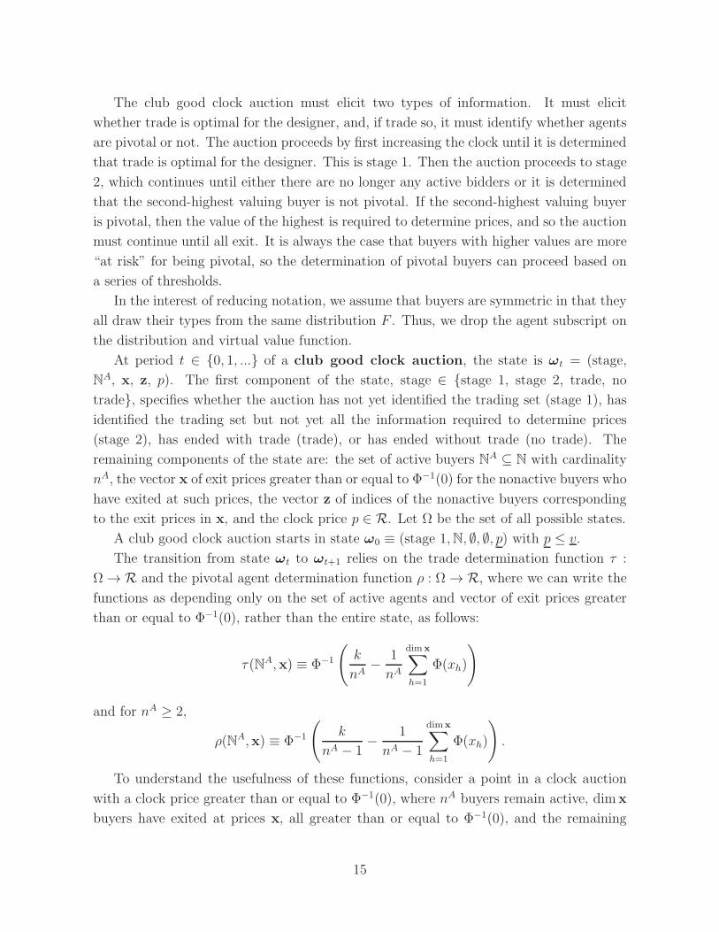
The club good clock auction must elicit two types of information. It must elicit

whether trade is optimal for the designer, and, if trade so, it must identify whether agents

are pivotal or not. The auction proceeds by first increasing the clock until it is determined

that trade is optimal for the designer. This is stage 1. Then the auction proceeds to stage

2, which continues until either there are no longer any active bidders or it is determined

that the second-highest valuing buyer is not pivotal. If the second-highest valuing buyer

is pivotal, then the value of the highest is required to determine prices, and so the auction

must continue until all exit. It is always the case that buyers with higher values are more

“at risk” for being pivotal, so the determination of pivotal buyers can proceed based on

a series of thresholds.

In the interest of reducing notation, we assume that buyers are symmetric in that they

all draw their types from the same distribution F . Thus, we drop the agent subscript on

the distribution and virtual value function.

At period t ∈ 0, 1, ... of a club good clock auction, the state is ωt = (stage,

NA, x, z, p). The first component of the state, stage ∈ stage 1, stage 2, trade, no

trade, specifies whether the auction has not yet identified the trading set (stage 1), has

identified the trading set but not yet all the information required to determine prices

(stage 2), has ended with trade (trade), or has ended without trade (no trade). The

remaining components of the state are: the set of active buyers NA ⊆ N with cardinality

nA, the vector x of exit prices greater than or equal to Φ−1(0) for the nonactive buyers who

have exited at such prices, the vector z of indices of the nonactive buyers corresponding

to the exit prices in x, and the clock price p ∈ R. Let Ω be the set of all possible states.

A club good clock auction starts in state ω0 ≡ (stage 1,N, ∅, ∅, p) with p ≤ v.

The transition from state ωt to ωt+1 relies on the trade determination function τ :

Ω → R and the pivotal agent determination function ρ : Ω → R, where we can write the

functions as depending only on the set of active agents and vector of exit prices greater

than or equal to Φ−1(0), rather than the entire state, as follows:

τ (NA,x) ≡ Φ−1

(

k

nA− 1

nA

dimx∑

h=1

Φ(xh)

)

and for nA ≥ 2,

ρ(NA,x) ≡ Φ−1

(

k

nA − 1− 1

nA − 1

dimx∑

h=1

Φ(xh)

)

.

To understand the usefulness of these functions, consider a point in a clock auction

with a clock price greater than or equal to Φ−1(0), where nA buyers remain active, dimx

buyers have exited at prices x, all greater than or equal to Φ−1(0), and the remaining

15

buyers have exited at prices less than Φ−1(0). If the nA active buyers continue to be

active at a clock price of τ (NA,x), then we can conclude that the condition for trade,∑

h∈I(v)Φ(vh) ≥ k, is satisfied. To see this, note that in this case, the set I(v) consists

of the dimx buyers with types x as well as the nA active buyers whose types are at least

τ(NA,x), which implies that

∑

h∈I(v)

Φ(vh) ≥dimx∑

h=1

Φ(xh)+nAΦ(τ (NA,x)) =dimx∑

h=1

Φ(xh)+nA

(

k

nA− 1

nA

dimx∑

h=1

Φ(xh)

)

= k,

which is the condition for trade.

Furthermore, if the condition for trade is satisfied and nA ≥ 2 active buyers continue

to be active at a clock price of ρ(NA,x), then we can conclude that no agent is pivotal.

To see this, note that for any active bidder l, if nA ≥ 2 so that there is at least one other

active bidder, then each active bidder’s virtual value is at least Φ(ρ(NA,x)), and so

∑

h∈I(v)\l

Φ(vh) ≥dimx∑

h=1

Φ(xh) + (nA − 1)Φ(ρ(NA,x))

=dimx∑

h=1

Φ(xh) + (nA − 1)

(

k

nA − 1− 1

nA − 1

dimx∑

h=1

Φ(xh)

)

= k,

so no such bidder is pivotal. Because the dimx bidders that exited at prices greater than

or equal to Φ−1(0) have lower values than the active bidders, none of those bidders is

pivotal either.

If the condition for trade is satisfied and nA = 1, then the final active bidder is pivotal

if and only if∑dimx

i=1 Φ(xi) < k. It is only necessary to have this final bidder reveal his

type if there are other pivotal bidders. It is sufficient to check whether the exited bidder

with the highest value would be pivotal if the active bidder’s value were equal to the

current clock price. The last bidder to exit may be pivotal if∑dimx−1

i=1 Φ(xi) + p < k. If

this is the case, we must continue to increase the clock price until either the final active

bidder exits or the last bidder to exit is revealed not to be pivotal. This is necessary in

the context of dominant strategy implementation because the designer needs to know the

values for all other trading bidders in order to determine the price for a pivotal bidder.

A club good clock auction continues until a state is reached that has a first component

equal to either “no trade” or “trade.” In the case of “no trade,” the auction ends with

no trade. In the case of “trade,” the auction ends with trade by the remaining active

bidders as well as by those identified in the vector z as exiting at prices at least Φ−1(0).

The prices are given by the pricing rule described below. The auction stays in stage 1

16

until either all buyers exit, in which case there is no trade, or the clock price reaches

the level specified by the trade determination function τ(NA,x) and moves to stage 2, in

which case there will be trade. The auction stays in stage 2 until either all buyers exit,

only 2 active buyers remain and the clock reaches the level specified by the pivotal agent

determination function ρ(NA,x), or only 1 active buyer remains but it is possible that the

second-highest valuing bidder might be pivotal.

• Stage 1: For t ∈ 0, 1, ..., if ωt = (stage 1,NA,x, z,p), then ωt+1 is determined as

follows:

If nA = 0, ωt+1 = (no trade,NA,x, z,p).

If nA > 0 and p < Φ−1(0), then increase the clock from p until either a buyer i exits

at clock price p ≤ Φ−1(0) or the clock reaches Φ−1(0) with no exit. If there is an

exit at p < Φ−1(0), define ωt+1 = (stage 1,NA\i,x, z, p), if there is an exit by buyer

i at Φ−1(0), define ωt+1 = (stage 1,NA\i, (x,Φ−1(0)), (z,i),Φ−1(0)), and otherwise

ωt+1 = (stage 1,NA,x, z,Φ−1(0)).

If nA > 0 and p ≥ Φ−1(0), then increase the clock from p until either a buyer i exits at

clock price p ≤ τ (NA,x) or the clock price reaches τ(NA,x) with no exit.7 If there

is an exit, define ωt+1 = (stage 1,NA\i, (x, p), (z,i),p), and otherwise ωt+1 = (stage

2,NA,x, z,p).

• Stage 2: For t ∈ 1, 2, ..., if ωt = (stage 2,NA,x, z,p), then ωt+1 is determined as

follows:

If nA = 0, ωt+1 = (trade,NA,x, z,p).

If nA ≥ 2, then increase the clock from p until either a buyer i exits at clock price p ≤ρ(NA,x) or the clock price reaches ρ(NA,x) with no exit. If there is an exit, define

ωt+1 = (stage 2,NA\i, (x, p), (z, i),p), and otherwise ωt+1 = (trade,NA,x, z,p).

If nA = 1:

If k ≤∑dimx−1i=1 Φ(xi) + Φ(p), then the second-highest valuing bidder is revealed not

to be pivotal, so the auction can end: ωt+1 = (trade,NA,x, z,p).

Otherwise, increase the clock from p until either the remaining buyer i exits at clock

price p ≤ Φ−1(k−∑dimx−1i=1 Φ(xi)) or the clock price reaches Φ−1(k−∑dimx−1

i=1 Φ(xi))

with no exit. If there is an exit, define ωt+1 = (trade,NA\i, (x, p), (z, i),p), andotherwise ωt+1 = (trade,NA,x, z,p).

7If the clock price is initially greater than or equal to the threshold, then the clock stops immediately.

17

• Pricing rule: For t ∈ 1, 2, ..., if ωt = (trade,NA,x, z,p), then buyers in T ≡ NA∪

z1 ∪ ... ∪ zdim z trade, with buyer l ∈ T paying ml(v,k), where v is defined by,

for l ∈ N,

vl ≡

v, if l /∈ T

p, if l ∈ NA

xi, otherwise, where l = zi.

Thus, conditional on using an increasing clock auction to implement the Bayesian

optimal club good mechanism in dominant strategies, this club good clock auction elicits

the minimum information required. That information includes sufficient detail about

types to discern whether∑

h∈I(v)Φh(vh) is greater than k or not, to determine whether

trade should occur, and sufficient detail about the types of trading agents to determine

which, if any, agents are pivotal and the corresponding price for any pivotal agents. For

example, if the types are such that no agent is pivotal, then the clock price stops at the

point when this is apparent and does not require full revelation of agents’ types, preserving

the privacy of high-valuing nonpivotal agents.

Incentives in the club good clock auction

Bidders in the club good clock auction have an incentive to exit at their values. Because

prices for trading agents are at least Φ−1(0) and because bidders who exit a prices less

than Φ−1(0) do not trade, a bidder with a value less than Φ−1(0) has an incentive to exit

at his value, and bidders with a value greater than or equal to Φ−1(0) have an incentive

to stay active at least until the price reaches Φ−1(0).

Case 1: vi ≥ Φ−1(0),∑

h∈I(v)Φ(vh) ≥ k, i is not pivotal: With truthful bidding, there is

trade and bidder i pays Φ−1(0). If bidder i exits at a price greater than Φ−1(0) but

less than vi or at a price greater than vi, then there is no change. Because there is

trade and i is not pivotal, a different exit point greater than Φ−1(0) does not affect

whether there is trade or whether i is pivotal.

Case 2: vi ≥ Φ−1(0),∑

h∈I(v)Φ(vh) ≥ k, i is pivotal: With truthful bidding, there

is trade and bidder i pays Φ−1(

k −∑h∈I−i(v)Φ(vh)

)

. If bidder i exits at a price

greater than Φ−1(0) but less than vi, then either their is no change or there is no

longer trade, in which case bidder i is worse off. If bidder i exits at a price greater

than vi, then there is still trade and bidder i is still pivotal, and so the amount

bidder i pays is unchanged.

Case 3: vi ≥ Φ−1(0),∑

h∈I(v)Φ(vh) < k: With truthful bidding, there is no trade. If

bidder i exits at a price less than vi, then there continues to be no trade. If bidder i

18

exits at a price greater than vi, either there is no change or bidder i becomes pivotal

and there is trade. In that case, bidder i pays Φ−1(

k −∑h∈I−i(v)Φ(vh)

)

. Because

for this case we assume, Φ(vi) < k −∑h∈I−i(v)Φ(vh), it follows that

Φ−1

k −∑

h∈I−i(v)

Φ(vh)

> Φ−1 (Φ(vi)) = vi,

and so deviator pays an amount greater than vi, implying that the deviation is not

profitable.

Thus, it is a dominant strategy for each bidder to exit the auction when the clock

price reaches his value. We summarize with the following proposition.

Proposition 3 The club good clock auction implements the Bayesian optimal club good

allocation in dominant strategies.

As defined by Li (2015), a strategy si is obviously dominant if, for any deviating

strategy s0, starting from any earliest information set where s0 and si disagree, the best

possible outcome from s0 is no better than the worst possible outcome from si. In the

club good clock auction, the strategy for a buyer of exiting at its value is not an obviously

dominant strategy.8

Privacy preservation in the club good clock auction

In the club good clock auction, we can show that the clock price never exceeds Φ−1(k),

so buyers with values greater than Φ−1(k) are never asked to reveal any more than the

fact that their value exceeds that threshold. The intuition for this result is that if the

clock price reaches Φ−1(k) with two or more active buyers, then it is revealed that the

condition for trade is satisfied and that no buyer is pivotal, and so the auction ends. If

the clock price reaches Φ−1(k) with only one active buyer, then it is again revealed that

the condition for trade is satisfied and that buyers other than the one active buyer are

not pivotal, so their purchase price is Φ−1(0). The purchase price for the one active buyer

is determined by the exit prices of the other buyers, which have already been revealed.

8Consider a buyer with value vi > Φ−1(0) who considers deviating by exiting at price v < vi. Supposethe clock price reaches v. Then the buyers’s payoff under the deviation will be qi(v,v−i)(vi − pi(v,v−i)).In the best possible outcome from the deviation, qi(v,v−i) = 1 and i is not pivotal and so pays Φ−1(0),for surplus of vi − Φ−1(0). At the information set in which the clock price is v, it may be unclear as towhether there will be trade. In particular, it may be that there is no trade even when buyer i exits at vi.Thus, the best possible outcome from exit at v exceeds the worst possible outcome from exit at vi fromthe perspective of that information set.

19

Thus, if the clock price reaches Φ−1(k), no further information is required to determine

whether the condition for trade is satisfied or the purchase prices of any of the buyers.

Formally, if nA ≥ 1, then the trade determination price is

τ (NA,x) = Φ−1

(

k

nA− 1

nA

dimx∑

h=1

Φ(xh)

)

≤ Φ−1

(

k

nA

)

≤ Φ−1 (k) ,

so the trade determination price never exceeds Φ−1(k). Thus, the clock price never exceeds

Φ−1(k) during stage 1 of the auction. In stage 2, as long as two or more buyers are active,

the clock price never exceeds ρ(NA,x), which is no greater than Φ−1(k):

ρ(NA,x) = Φ−1

(

k

nA − 1− 1

nA − 1

dimx∑

h=1

Φ(xh)

)

≤ Φ−1

(

k

nA − 1

)

≤ Φ−1 (k) .

Finally, if nA = 1 in stage 2 of the auction, then the clock price does not exceed Φ−1(k −∑dimx−1

i=1 Φ(xi)) ≤ Φ−1(k). Thus, the clock price never exceeds Φ−1(k).

We summarize in the following proposition.

Proposition 4 The club good clock auction is privacy preserving for all buyers with val-

ues greater than Φ−1(k).

4.2 Two sided: Revenue sharing contracts

In a variety of real-world situations, intermediaries who enable trade between producers

and buyers of club goods may need to contract with the producer before buyers are

present. Most naturally, this occurs when production precedes sales and marketing, for

example because of the innovative nature of the good, as would typically be the case

with works of art. We next show that this variation in the timing of events changes

the intermediary’s mechanism design problem from a club good problem to a standard

procurement problem even though it does not affect the nonrivalrous nature of the good

in question. We also show that it gives raise to a contractual arrangement that is widely

used in practice, for example, by iTunes for songs and e-books, namely shared revenue

between the intermediary and the seller.

To be specific, we suppose that the intermediary and the seller have to contract in

stage 1 before any buyer arrives in stage 2. There is no loss in generality by assuming

that there is no discounting, as will be shown shortly. Let n be the number of buyers who

draw their types independently from the regular distribution F . To conserve on notation,

for x ≥ Γ(k), define Γ−1(x) to be k.

20

From Propositions 1 and 2, we know that it is optimal to sell the good as a club good.

Denote the maximizer of x(1−F (x)) over x by Φ−1(0). The maximized expected per buyer

revenue is thus Φ−1(0)(1−F (Φ−1)). Let R denote expected revenue from stage 2.9 With

this seemingly innocuous change in assumptions, the intermediary’s problem becomes a

standard procurement problem, with the willingness to pay of the risk-neutral, patient

intermediary being given by R. Facing a seller whose cost k is drawn from the regular

distribution G with virtual cost Γ(k), the intermediary-optimal mechanism consists of

the take-it-or-leave-it offer to the seller pS ≡ Γ−1(R), as is well known from standard

mechanism design theory.

Under the assumptions that the support of G is [0, k] and that G(k) is a generalized

Pareto distribution of the form G(k) = (k/k)σ,10 we have Γ−1(k) = σk/(σ + 1) and

pS =σ

σ + 1R.

That is, the optimal take-it-or-leave-it offer is a percentage of revenue. Interestingly, rather

than setting a take-it-or-leave-it offer, the intermediary can equivalently implement this

optimal contract by offering the percentage σ/(σ + 1) of realized revenue. Moreover, as

long as the intermediary and the seller are equally informed about demand and both

believe that buyers draw their types independently from F , it is immaterial whether the

intermediary or the seller sets the buyers’ price pB = Φ−1(0). Thus, under the assumption

of a generalized Pareto distribution, the predictions of this model are consistent with

Apple’s controversial e-books contracting model. This consisted of a revenue sharing

agreement with publishers that left the authority to set the buyers’ prices with the sellers.

On the surface, this arrangement may appear to be different from Apple’s business model

for songs and movies on iTunes, which also involves revenue sharing but leaves the right

to set buyers’ prices with Apple. However, as observed by Loertscher and Niedermayer

(2008) in the context of private goods, the broker-optimal fee is independent of the buyers’

distribution F if the seller’s distribution is a generalized Pareto distribution. Therefore,

it does not even matter whether the intermediary and the seller are equally well informed

about demand.

The result that the optimal procurement contract can be implemented with a fee levied

on realized revenue generalizes to seller’s type distributions of the form G(k) =(

k−k

k−l

)σ

.

As shown by Loertscher and Niedermayer (2008), these distributions are equivalent to

linear virtual cost functions Γ(k) = σk+1−kσ

. This linearity obviously implies linearity of

9All that matters in this setup is expected discounted future revenue, which is why the assumptionthat there is no discounting is without loss. If the discount factor were some δ > 0 and expected stage 2revenue were R, we would simply have R = δR.

10See Loertscher and Niedermayer (2015) for a micro-foundation for why generalized Pareto distribu-tions may be a particularly good approximation of the supply side in thin markets.

21

the inverse virtual cost function: Γ−1(y) = σy+kσ+1

. Any risk-neutral seller will be indifferent

between receiving pS or E[Γ−1(Y )] if and only if Γ−1 is linear, where Y is realized revenue,

whose distribution is such that R = E[Y ]. As before, whether the seller or the interme-

diary sets the reserve price buyers face is immaterial. These results are related to but

distinct from the observations of Loertscher and Niedermayer (2008, 2015), who analyze

intermediary-optimal auctions for a seller of a private good. They notice that for this

family of distributions, the optimal fee function is linear and independent of the buyers’

distribution. With a private good, however, the seller has to set the reserve price the

buyers face because the optimal reserve price varies with the seller’s private information

about his cost.

5 Asymptotics in the two-sided setup

In some two-sided setups, it is reasonable to think of the number of buyers as being very

large, for example for iTunes and other digital products. Thus, we consider the asymptotic

properties of our mechanisms. For the purposes of this section, for simplicity assume that

buyers are symmetric.

Schmitz (1997) provides asymptotic results for the one-sided setup. He allows the

number of buyers to go to infinity and assumes, as in Rob (1989) that kn = κn, where

κ ∈ (0, 1). Schmitz (1997, Proposition 3) shows that in the optimal mechanism the

club good is provided if and only if E [max0,Φ(vi)] ≥ κ, which implies that when this

condition holds, the club good is provided with probability one in the limit. This is in

contrast to the results of Rob (1989) and Mailath and Postlewaite (1990) for the case of

nonexcludable public goods. They show that in their setup, the good is provided with

probability zero in the limit.

We extend this result to the two-sided setup. We assume that the cost when there

are n buyers is kn ≡ κnk, where κ ∈ (0, 1) and k is drawn from distribution G. Thus, kn

has distribution H(kn) ≡ G(kn/(nκ)) on [κnk, κnk] with density h(kn) =1nκg(kn/(nκ)).

Then the weighted virtual cost associated with distribution H is Γ(kn) ≡ kn + αH(kn)h(kn)

=

kn + αnκG(kn/(nκ))h(kn/(nκ))

, and so Γ(kn) = nκΓ(kn/(nκ)) = nκΓ(k).

Under this assumption, in the two-sided case, when there are n buyers it is optimal

22

for the good to be provided if and only if∑

h∈I(v)Φh(vh) ≥ Γ(kn). Note that

limn→∞Pr(

∑

h∈I(v)Φ(vh) ≥ Γ(kn))

= 1

⇔ limn→∞Pr(

∑

h∈I(v)Φ(vh) ≥ nκΓ(k))

= 1

⇔ limn→∞Pr(

1Γ(k)

1n

∑

h∈I(v) Φ(vh) ≥ κ)

= 1

⇔ limn→∞E[

1Γ(k)

1n

∑

h∈I(v)Φ(vh)]

≥ κ

⇔ limn→∞E[

1Γ(k)

1n

∑ni=1max0,Φ(vi)

]

≥ κ

⇔ E[

1Γ(k)

]

limn→∞E[

1n

∑ni=1max0,Φ(vi)

]

≥ κ

⇔ E [max0,Φ(v)] ≥ κE [Γ(k)] .

Thus, we have the following result.

Proposition 5 In the optimal mechanism in the two-sided setup, the club good is provided

with probability one in the limit as the number of buyers goes to infinity and k = κn, where

κ ∈ (0, 1), if and only if E [max0,Φ(v)] ≥ κE [Γ(k)].

Thus, under the condition of Proposition 5, the club good intermediary facilitates

trade with probability one in the limit. Using E[max0,Φ(v)] = Φ−1(0)(1− F (Φ−1(0)))

and E [Γ(k)] = k,11 we can restate the necessary and sufficient condition of Proposition 5

as

Φ−1(0)(1− F (Φ−1(0))) ≥ κk.

For example, with values drawn from the uniform distribution on [0, 1] and k = 1, the

condition is κ ≤ 14.

6 Extensions

6.1 Congestion effects

We consider two types of congestion effects, those with costs borne by the seller and those

that diminish the value to buyers.

We allow for the possibility that the seller incurs incremental costs to support addi-

tional buyers by assuming that if the designer allocates the good to ℓ buyers, then the

seller’s cost is k + c(ℓ), where k is drawn from distribution G and c(·) is a nonnegative

nondecreasing function with c(0) = 0. Thus, the cost of the first unit is k + c(1) and

11These follow using E[max0,Φ(v)] =∫ v

vmax0,Φ(v)f(v)dv =

∫ v

Φ−1(0)

(

v − 1−F (v)f(v)

)

f(v)dv and

E [Γ(k)] =∫ k

k

(

k + G(k)g(k)

)

g(k)dk and using integration by parts.

23

the incremental cost associated with selling ℓ units rather than one unit is c(ℓ) − c(1).

The case of c(·) ≡ 0 corresponds to no congestion costs for the seller. Given ℓ, the

seller’s cost k + c(ℓ) has distribution G(x; ℓ) ≡ G(x − c(ℓ)), with associated virtual cost

Γ(x; ℓ) ≡ x+ G(x;ℓ)g(x;ℓ)

= x+ G(x−c(ℓ))g(x−c(ℓ))

, so Γ(k+ c(ℓ); ℓ) = Γ(k) + c(ℓ). Thus, we can view the

seller as having virtual cost Γ(k) + c(ℓ).

We also allow for the possibility that buyers’ values are diminished by increases in the

number of buyers by assuming that buyer i with type vi has value viθ(ℓ) for the good if

the good is supplied to ℓ buyers, where θ(·) is a nonincreasing function with value in [0, 1]

and θ(1) = 1. The case of θ(·) ≡ 1 corresponds to no congestion costs for buyers.

In any incentive compatible interim individually rational mechanism the designer’s

expected profit is

Π = Ev,k

[

n∑

i=1

Φi(vi)θ

(

n∑

j=1

qj(v, k)

)

qi(v, k)− Γ(k)min

1,n∑

i=1

qi(v, k)

− c

(

n∑

i=1

qi(v, k)

)]

,

minus a constant, which, as before, can be set equal to 0 by making the individual

rationality constraints bind for the worst-off types.

Recall that I(v) ≡

i : vi ≥ Φ−1i (0)

. Relabel the buyers in I(v) as 1, ..., |I(v)| so that

Φ1(v1) ≥ ... ≥ Φ|I(v)|(v|I(v)|), breaking ties at random. Relabel the buyers not in I(v) with

indices greater than |I(v)|. If I(v) = ∅, let q = 0 and otherwise let q be such that

q ∈ arg maxh∈1,...,|I(v)|

h∑

i=1

Φi(vi)θ (h)− c (h) .

Thus, allocation of the object to (relabelled) buyers 1, ..., q maximizes the sum of the

congestion adjusted virtual values of the trading buyers. The pointwise maximum requires

trade with buyers 1, ..., q if and only if trade with these buyers is optimal for the designer:

qi(v, k) ≡

1, if i ≤ q and∑q

h=1Φh(vh)θ (q)− Γ(k)− c (q) ≥ 0

0, otherwise.

In the dominant strategy implementation, agents pay the lowest type they could report

and yet still trade.

In some situations, congestion costs may be constant marginal costs that are borne

by the intermediary. For example, in the case of digital goods like songs, books, and

movies, costly server capacity is provided by the broker. If the intermediary and the

seller contract before buyers arrive, as assumed in Section 4.2, then the intermediary-

optimal contract will still be a take-it-or-leave-it offer pS = Γ−1(Rnet), with the twist that

Rnet is now expected net revenue. If, in addition, the seller’s virtual type function is

24

linear, the intermediary-optimal contract can be implemented with a linear fee function

of realized net revenue Y net that satisfies Rnet = E[Y net].

6.2 The case without regularity

If the virtual types are not monotone, then we must “iron.” Given distribution Fi with

positive density fi (implying that Fi is invertible) and nonmonotone virtual value Φi,

the ironed virtual value Φi is defined as follows: Let κi(x) ≡ Φi(F−1i (x)) and let Ki(x) ≡

∫ x

vκi(y)dy and let Kco

i (x) define the convex hull of Ki(x) on [v, v]. Define κi(x) ≡ Kco′i (x).

Then the ironed virtual value is

Φi ≡ κi(Fi(x)).

For example, consider

F (x) ≡

3/2 x, if 0 ≤ x ≤ 1/2

1/2 + 1/2 x, if 1/2 < x ≤ 1

on [0, 1]. Then the virtual value is nonmonotone, as shown in Figure 5(a). We show the

construction of κ and K and its convex hull in Figures 5(b) and 5(c). The original and

ironed virtual values are shown in Figure 5(d).

The Bayesian optimal club good mechanism and CGCA are then as defined above,

but replacing the virtual types with ironed the virtual types and replacing the inverse of

the virtual types with the generalized inverse:

Φ−1

i (x) ≡ inf

vi ∈ [v, v] | Φi(vi) ≥ x

.

In the private good environment, ironing introduces a need for tie breaking because buyers

with different values can have the same ironed virtual type. In a rivalrous environment,

tie breaking arises with positive probability when regularity is not satisfied. However, in

a club good setting, if one buyer with a particular virtual type trades at a given price,

then all buyers with that virtual type also trade at that same price, so tie breaking is not

necessary.

7 Conclusions

The emergence of the internet and of digital goods have renewed interest in the optimal

mechanisms for the provision of public goods with exclusion, also known as club goods.

Because digital goods like e-books, songs, and movies are typically traded via interme-

diaries such as Amazon, iTunes, and Netflix, a new question of considerable practical

25

(a) Virtual value (b) κ

(c) K and Kco (d) Ironed and unironed virtual values

Figure 5: Illustration of the ironing of the virtual value

relevance is what pricing mechanisms are optimal for a club good intermediary. In this

paper, we have analyzed this question using a Bayesian mechanism design framework

with independent private values, which beyond incentive compatibility and individual

rationality imposes no constraints on the choice of mechanism.

Dynamics are an important aspect of real life that are not captured by our model. In

many situations, not all buyers are present at the outset when the production decisions

have to be made. Extending our one-shot model to a dynamic setup that incorporates

features like these seems a valuable avenue for future research. Crowdfunding and crowd-

funding platforms are another example in which uncertainty about aggregate demand,

which is only lifted over time, is arguably important. Dynamics also play a pertinent role

in the economics of innovation and R&D, with ideas being a quintessential example of a

consumption good without rivalry and patents being one way of making this sort of public

good excludable. In this vein, one might consider the optimal mechanism in a setup in

which the seller first has to invest, for example developing new drug or producing a new

movie (with effort being noncontractible). One can then consider how large is the optimal

weight on seller profit in this environment.

26

A Appendix: Standard arguments

As stated in the text, standard arguments imply that in any incentive compatible interim

individually rational mechanism the designer’s expected profit is

Π = Ev,k

[

n∑

i=1

Φi(vi)qi(v,k)− Γ(k)min

1,

n∑

i=1

qi(v,k)

]

minus a constant, which, however, can be set equal to 0 by making the individual ratio-

nality constraints bind for the worst-off types.

By the Revelation Principle, we can focus attention on direct mechanisms (q,m,mS),

where q : ×ni=1[v, v]×[k, k] → ×n

i=1[0, 1],m : ×ni=1[v, v]×[k, k] → Rn, andmS : ×n

i=1[v, v]×[k, k] → R. This differs from the private good case in that q maps into ×n

i=1[0, 1], whereas

in the private good case it maps into the n-dimensional simplex. The expected quantity

produced by the seller is qS(v, k) ≡ 1−Πni=1(1− qi(v,k)). The proof provided by Krishna

(2002, Proposition 5.1) for the private good case is easily adapted to our club good

environment. The following arguments, which are standard for the private good case

(see, e.g., Krishna, 2002, Chapter 5.1), apply equally to the club good case.

Given a direct mechanism (q,m,mS) and letting f(v) ≡ f1(v1) · · · fn(vn), define

qi(zi) =

∫

[k,k]

∫

×j 6=i[v,v]

qi(zi,v−i, k)f−i(v−i)g(k)dv−idk

to be the probability that i gets the object when he reports zi and all other buyers and

the seller report their types truthfully. Similarly, define

mi(zi) =

∫

[k,k]

∫

×j 6=i[v,v]

mi(zi,v−i, k)f−i(v−i)g(k)dv−idk

to be buyer i’s expected payment when he reports zi and others report truthfully. Because

we assume independent draws, qi(zi) and mi(zi) depend only on the report zi and not on

the buyer i’s true value vi. The expected payoff of buyer i is then qi(zi)vi − mi(zi).

Similarly, define the expected quantity and payment to the seller to be

qS(k) =

∫

×ni=1

[v,v]

qS(v, k)f(v)dv

and

mS(k) ≡∫

×ni=1

[v,v]

mS(v, k)f(v)dv.

27

The direct mechanism is incentive compatible if for all i, xi, and zi,

Ui(vi) ≡ qi(vi)vi − mi(vi) ≥ qi(zi)vi − mi(zi)

and for all k and k′,

US(k) ≡ mS(k)− kqS(k) ≥ mS(k′)− kqS(k′).

Focusing on the buyers, this implies that Ui(vi) = maxzi∈[v,v] qi(zi)vi − mi(zi) , i.e.,Ui is a maximum of a family of affine functions, which implies that Ui is convex and so

absolutely continuous and differentiable almost everywhere in the interior of its domain.12

In addition, incentive compatibility implies that Ui(zi) ≥ qi(vi)zi − mi(vi) = Ui(vi) +

qi(vi)(zi − vi), which for δ > 0 implies

Ui(vi + δ)− Ui(vi)

δ≥ qi(vi)

and for δ < 0 impliesUi(vi + δ)− Ui(vi)

δ≤ qi(vi),

so taking the limit as δ goes to zero, at every point vi where Ui is differentiable, U′i(vi) =

qi(vi). Because Ui is convex, this implies that qi(vi) is nondecreasing.13 Because every

absolutely continuous function is the definite integral of its derivative,

Ui(vi) = Ui(v) +

∫ vi

v

qi(ti)dti,

which implies that, up to an additive constant, a buyer’s expected payoff in an incentive

compatible direct mechanism depends only on the allocation rule.

Turning to the seller, US(k) = maxk′∈[k,k]

mS(k′)− kqS(k′)

, implying, as with the

buyers, that US is convex and so absolutely continuous and differentiable almost every-

where in the interior of its domain. In addition, at every point k where US is differentiable,

12A function f : [v, v] → R is absolutely continuous if for all ε > 0 there exists δ > 0 such thatwhenever a finite sequence of pairwise disjoint sub-intervals (vk, v

′k) of [v, v] satisfies

∑

k(v′k − vk) < δ,

then∑

k |f(v′k)− f (vk)| < ε. One can show that absolute continuity on compact interval [a, b] impliesthat f has a derivative f ′ almost everywhere, the derivative is Lebesgue integrable, and that f(x) = f(a)+∫ x

af ′(t)dt for all x ∈ [a, b]. For example, the Cantor function is uniformly continuous but not absolutely

continuous (the derivative of the Cantor function is zero almost everywhere and so 0 =∫ 1

0F ′(t)dt <

F (1)− F (0) = 1).13To see that a nondecreasing qi implies incentive compatibility, note that a sufficient condition for

incentive compatibility is that for all vi and zi, Ui(zi) ≥ Ui(vi) + qi(vi)(zi − vi), which because everyabsolutely continuous function is the definite integral of its derivative, we can write as

∫ zi

viqi(ti)dti ≥

qi(vi)(zi − vi), which holds if qi is nondecreasing.

28

US′(k) = qS(k), and this is nondecreasing. Finally, again as above, we can write

US(k) = US(k) +

∫ k

k

qS(k′)dk′.

Thus, the usual Revenue Equivalence result for private goods applies here: If the direct

mechanism (q,m,mS) is incentive compatible, then for all i and vi, the expected payment

by buyer i is

mi(vi) = qi(vi)vi − Ui(vi)

= qi(vi)vi − Ui(v)−∫ vi

v

qi(ti)dti

= mi(v)− qi(v)v + qi(vi)vi −∫ vi

v

qi(ti)dti

and the expected payment to the seller is

mS(k) = US(k)− kqS(k)

= US(k) +

∫ k

k

qS(k′)dk′ − kqS(k)

= mS(k)− qS(k)k +

∫ k

k

qS(k′)dk′ − kqS(k).

If the worst-valuing type never trades, and so by individual rationality pays zero, then

we have

mi(vi) = qi(vi)vi −∫ vi

v

qi(ti)dti (16)

and

mS(k) =

∫ k

k

qS(k′)dk′ − kqS(k). (17)

29

The seller’s expected revenue from buyer is then

n∑

i=1

Ev[mi(vi)] =

n∑

i=1

∫ v

v

mi(vi)fi(vi)dvi

=

n∑

i=1

∫ v

v

(

qi(vi)vi −∫ vi

v

qi(ti)dti

)

fi(vi)dvi

=

n∑

i=1

(∫ v

v

qi(vi)vifi(vi)dvi −∫ v

v

∫ v

ti

qi(ti)fi(vi)dvidti

)

=n∑

i=1

(∫ v

v

qi(vi)vifi(vi)dvi −∫ v

v

qi(ti) (1− Fi(ti)) dti

)

=

n∑

i=1

∫ v

v

qi(vi)

(

vi −1− Fi(vi)

fi(vi)

)

fi(vi)dvi

=n∑

i=1

∫ v

v

qi(vi)Φi(vi)fi(vi)dvi

= Ev

[

n∑

i=1

qi(vi)Φi(vi)

]

,

where the first equality uses the definition of the expectation, the second uses (16), the

third switches the order of integration, the fourth integrates, the fifth collects terms, the

sixth uses the definition of the virtual value Φi, and the last equality uses the definition

of the expectation.

Applying similar steps, and using (17), one can show that

Ek

[

mS(k)]

= Ek

[

Γ(k)qS(k)]

.

Thus, we have the result that

Π = Ev,k

[

n∑

i=1

Φi(vi)qi(v,k)− Γ(k)qS(k)

]

.

30

References

Bergemann, D., and S. Morris (2005): “Robust Mechanism Design,” Econometrica,

73(6), 1771–1813.

Bulow, J., and J. Roberts (1989): “The Simple Economics of Optimal Auctions,”

Journal of Political Economics, 97(5), 1060–90.

Caillaud, B., and B. Jullien (2001): “Competing Cybermediaries,” European Eco-

nomic Review, 45, 797–808.

(2003): “Chicken and Egg: Competition among Intermediation Service

Providers,” RAND Journal of Economics, 34(2), 309–328.

Fang, H., and P. Norman (2010): “Optimal Provision of Multiple Excludable Public

Goods,” American Economic Journal: Microeconomics, 2(4), 1–37.

Gehrig, T. (1993): “Intermediation in Search Markets,” Journal of Economics & Man-

agement Strategy, 2, 97–120.

Gomes, R. (2014): “Optimal Auction Design in Two-Sided Markets,” Rand Journal of

Economics, 45, 248–272.

Hagerty, K., and W. Rogerson (1987): “Robust Trading Mechanisms,” Journal of

Economic Theory, 42, 94–107.

Hellwig, M. F. (2010): “Utilitarian Mechanism Design for an Excludable Public Good,”

Economic Theory, 44, 361–397.

Kagel, J. H. (1995): “Auctions: A Survey of Experimental Research,” in The Handbook

of Experimental Economics, ed. by J. H. Kagel, and A. E. Roth, pp. 501–585. Princeton

University Press, Princeton, NJ.

Krishna, V. (2002): Auction Theory. Elsevier Science, Academic Press.

Ledyard, J. O. (1986): “The Scope of the Hypothesis of Bayesian Equilibrium,” Journal

of Economic Theory, 39(1), 59–82.

Ledyard, J. O., and T. R. Palfrey (2007): “A General Characterization of Interim

Efficient Mechanisms for Independent Linear Environments,” Journal of Economic The-

ory, 133, 441–466.

Li, S. (2015): “Obviously Strategy-Proof Mechanisms,” Working Paper, Stanford Uni-

versity.

31

Loertscher, S. (2007): “Horizontally Differentiated Market Makers,” Journal of Eco-

nomics & Management Strategy, 16(4), 793–825.

(2008): “Market Making Oligopoly,” Journal of Industrial Economics, 56(2),

263–289.

Loertscher, S., and L. M. Marx (2015): “Prior-Free Bayesian Optimal Double-Clock

Auctions,” Working Paper, University of Melbourne.

Loertscher, S., and A. Niedermayer (2008): “Fee-Setting Intermediaries: On Real

Estate Agents, Stock Brokers, and Auction Houses,” Discussion Paper # 1472, North-

western University.

(2015): “Percentage Fees in Thin Markets: An Optimal Pricing Perspective,”

Working Paper, University of Mannheim and University of Melbourne.

Mailath, G. J., and A. Postlewaite (1990): “Asymmetric Information Bargaining

Problems with Many Agents,” Review of Economic Studies, 57(3), 351–367.

Marwell, N. B. (2015): “Competing Fundraising Models in Crowdfunding Markets,”

Working Paper, University of Wisconsin-Madison.

Milgrom, P., and I. Segal (2015): “Deferred-Acceptance Auctions and Radio Spec-

trum Reallocation,” Working Paper, Stanford University.

Mookherjee, D., and S. Reichelstein (1992): “Dominant Strategy Implementation

of Bayesian Incentive Compatible Allocation Rules,” Journal of Economic Theory, 56,

378–399.

Myerson, R., and M. Satterthwaite (1983): “Efficient Mechanisms for Bilateral

Trading,” Journal of Economic Theory, 29(2), 265–281.

Myerson, R. B. (1981): “Optimal Auction Design,” Mathematical Operations Research,

6(1), 58–73.

Norman, P. (2004): “Efficient Mechanisms for Public Goods with Use Exclusions,”

Review of Economic Studies, 71(4), 1163–1188.

Rob, R. (1989): “Pollution Claim Settlements under Private Information,” Journal of

Economic Theory, 47(2), 307–333.

Rochet, J.-C., and J. Tirole (2002): “Cooperation Among Competitors: Some Eco-

nomics of Payment Card Associations,” Rand Journal of Economics, 33(4), 549–570.

32

(2006): “Two-Sided Markets: A Progress Report,” RAND Journal of Economics,

37(3), 645–667.

Rubinstein, A., and A. Wolinsky (1987): “Middlemen,” Quarterly Journal of Eco-

nomics, 102(3), 581–593.

Rust, J., and G. Hall (2003): “Middlemen versus Market Makers: A Theory of Com-

petitive Exchange,” Journal of Political Economy, 111(2), 353–403.

Schmitz, P. W. (1997): “Monopolistic Provision of Excludable Public Goods under

Private Information,” Public Finance, 52(1), 89–101.

Spulber, D. F. (1996): “Market Making by Price-Setting Firms,” Review of Economic

Studies, 63(4), 559–580.

Stahl, D. O. (1988): “Bertrand Competition for Inputs and Walrasian Outcomes,”

American Economic Review, 78(1), 189–201.

Strausz, R. (2015): “Crowdfunding, Demand Uncertainty, and Moral Hazard – A Mech-

anism Design Approach,” SFB 649 Discussion Paper 2015-036.

Wilson, R. (1987): “Game Theoretic Analysis of Trading Processes,” in Advances in

Economic Theory, ed. by T. Bewley, pp. 33–70. Cambridge University Press, Cam-

bridge, U.K.

33