cluster analysis (revised 6-2014) - ndsuhzau).pdf · •...
TRANSCRIPT

CLUSTER ANALYSIS
Introduction
• Cluster analysis is a technique for grouping individuals or objects hierarchically into unknown groups suggested by the data.
• Cluster analysis can be considered an alternative to Factor Analysis.
• Cluster analysis differs from discriminant analysis.
o In cluster analysis the group membership is unknown prior to the analysis.
• In the biological sciences, an area where cluster analysis has been widely used is taxonomy.
o In taxonomy individuals are classified into arbitrary groups based on measurements of the individuals.
o The classification moves from the most general to the most specific.
Kingdom Phylum Subphylum Class Order Family Genus Species
• In economics, cluster analysis can be used for data mining.
o For example, in a market survey you could classify patrons into groups based on their answers to many questions.
• Warnings for cluster analysis.
o Groupings from cluster analysis can be different based on the method of analysis used.
o Since the groups are not known a priori, it can be difficult to determine if the results make sense in the context of the research being conducted.
o Knowledge of the population you are sampling and common sense are two important tools when it comes to interpreting results from cluster analysis.
Basic Concepts of Cluster Analysis
• Cluster analysis can be divided into two basic steps,
1. Initial analysis of data.
2. Analytical clustering using one of many methods of amalgamation. Initial analysis
o It is always a good idea before any statistical analysis to plot a scatter diagram of your data to see if there are any irregularities that need to be address using a transformation.
o A common transformation in multivariate analyses is to “standardize” your data so that it has a mean of 0 and a variance of 1.0
𝑆𝑡𝑎𝑛𝑑𝑎𝑟𝑑𝑖𝑧𝑒𝑑 𝑌! =(𝑌! − 𝑌)𝑆!
o If in visualizing your data you seem to see clusters that are elliptical in shape,
you want to use a transformation method that will make the resultant pooled within cluster covariance matrix spherical. v The method PROC ACELUS (Approximate Covariance Estimation for
Clustering) procedure in SAS will perform the transformation.
v Neither cluster membership nor the number of clusters needs to be known. Analytical clustering
Distance Measures o Distance measures can be studied in large data sets to determine similarities
or clusters.
o The opposite of similarity is distance.
o Distance values can be calculated for each pair of observations.
o Statistical methods to calculate distance are very sensitive to outliers. So you are encouraged to run diagnostics on your data to identify outliers and remove them if necessary.

o The most commonly used distance measurement is the Euclidian Distance.
Distance (x,y) =Σ!(𝑥! − 𝑦!)!
o Different methods to determine distance will provide different results.
Cluster Analysis Process o In the initial cluster analysis, all individuals begin in the same cluster.
o In subsequent rounds of analyses, the entries are placed into more and more
clusters.
o At the end of the cluster analysis, all individuals are in their own cluster.
o During the various rounds of cluster analysis, the distances between new clusters must be determined and we need to be ale to determine when two clusters are sufficiently close to be linked together.
o Two of the most common methods of cluster analysis are,
§ Unweighted Pair-‐Group Mean Average (UPGMA): the distance
between any two clusters is the average distance between all individuals in the different clusters.
§ Ward’s Method: a minimum variance method that uses an ANOVA approach. The method tries to minimize the sum of squares of any two clusters that are formed at each step of the cluster analysis.
Estimating the Number of Clusters
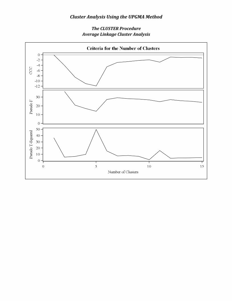
o Three methods that can be used to estimate the number of clusters are the, 1. Cubic clustering criterion (CCC) method: the estimated number of clusters occurs at the start of a peak on the graph . There may be more than one peak per plot.
2. Pseudo F: estimated number of clusters occurs at the start of peaks on the graph. There may be more than one peak per plot.
3. t2 The graph is read right to left. The estimated number of
clusters occurs at the start of a peak. There may be more than one peak per plot.
Precautions When Using Cluster Analysis
• Unless there is considerable separation between inherent groups when you view the scatter plots, it is not realistic to expect Cluster Analysis to provide clear results.
• Cluster Analysis is very sensitive to outliers.
• Results from the different Cluster Analysis methods may give you very different results.
• If you have large amounts of data, one method of simple validation of the results
from Cluster Analysis is to conduct the analysis on the two halves of your data. It would be preferable to select the individuals to be assigned to the two halves at random.
Example of Cluster Analysis • In this example, I am using data from one of my students’ (Sintayehu Daba) PhD
dissertation. Sintayehu is evaluating barley lines from three regions, Ethiopia and Kenya, ICARDA, and North Dakota, USA. Sintayehu collected data on many different plant characters, agronomic traits, and disease resistance. In the analysis, I am trying to determine if cluster analysis will successfully separate the data into distinct clusters based on the data collected.
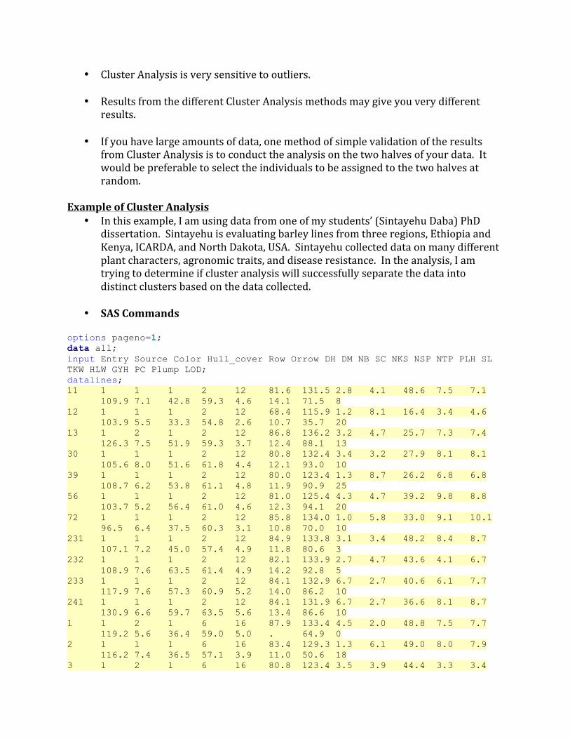
• SAS Commands
options pageno=1; data all; input Entry Source Color Hull_cover Row Orrow DH DM NB SC NKS NSP NTP PLH SL TKW HLW GYH PC Plump LOD; datalines; 11 1 1 1 2 12 81.6 131.5 2.8 4.1 48.6 7.5 7.1 109.9 7.1 42.8 59.3 4.6 14.1 71.5 8 12 1 1 1 2 12 68.4 115.9 1.2 8.1 16.4 3.4 4.6 103.9 5.5 33.3 54.8 2.6 10.7 35.7 20 13 1 2 1 2 12 86.8 136.2 3.2 4.7 25.7 7.3 7.4 126.3 7.5 51.9 59.3 3.7 12.4 88.1 13 30 1 1 1 2 12 80.8 132.4 3.4 3.2 27.9 8.1 8.1 105.6 8.0 51.6 61.8 4.4 12.1 93.0 10 39 1 1 1 2 12 80.0 123.4 1.3 8.7 26.2 6.8 6.8 108.7 6.2 53.8 61.1 4.8 11.9 90.9 25 56 1 1 1 2 12 81.0 125.4 4.3 4.7 39.2 9.8 8.8 103.7 5.2 56.4 61.0 4.6 12.3 94.1 20 72 1 1 1 2 12 85.8 134.0 1.0 5.8 33.0 9.1 10.1 96.5 6.4 37.5 60.3 3.1 10.8 70.0 10 231 1 1 1 2 12 84.9 133.8 3.1 3.4 48.2 8.4 8.7 107.1 7.2 45.0 57.4 4.9 11.8 80.6 3 232 1 1 1 2 12 82.1 133.9 2.7 4.7 43.6 4.1 6.7 108.9 7.6 63.5 61.4 4.9 14.2 92.8 5 233 1 1 1 2 12 84.1 132.9 6.7 2.7 40.6 6.1 7.7 117.9 7.6 57.3 60.9 5.2 14.0 86.2 10 241 1 1 1 2 12 84.1 131.9 6.7 2.7 36.6 8.1 8.7 130.9 6.6 59.7 63.5 5.6 13.4 86.6 10 1 1 2 1 6 16 87.9 133.4 4.5 2.0 48.8 7.5 7.7 119.2 5.6 36.4 59.0 5.0 . 64.9 0 2 1 1 1 6 16 83.4 129.3 1.3 6.1 49.0 8.0 7.9 116.2 7.4 36.5 57.1 3.9 11.0 50.6 18 3 1 2 1 6 16 80.8 123.4 3.5 3.9 44.4 3.3 3.4

105.1 7.0 39.0 59.0 3.4 9.7 74.9 15 4 1 1 1 6 16 85.7 132.9 2.9 2.8 49.1 6.1 6.1 105.6 5.2 40.2 59.9 3.6 10.7 72.2 8 5 1 1 1 6 16 83.2 128.7 2.4 7.3 47.0 5.7 5.4 104.7 5.2 35.0 54.8 3.3 11.5 65.5 15 6 1 1 1 6 16 85.4 132.4 4.7 2.2 34.0 10.0 11.0 130.2 8.0 45.8 57.0 5.5 11.7 59.6 5 7 1 1 1 6 16 83.0 126.4 2.3 3.7 44.2 6.8 5.8 107.7 9.2 44.6 60.2 4.8 13.1 84.2 5
.
.
.
. 89.5 7.6 36.1 59.0 2.5 9.6 64.5 0 82 5 1 1 2 52 79.9 131.3 1.1 7.9 23.9 11.6 12.1 80.6 6.9 35.2 60.3 2.1 10.3 66.5 0 227 5 1 1 2 52 86.2 138.9 1.1 8.1 27.6 7.2 7.7 78.3 6.8 35.4 58.9 2.1 9.3 50.8 1 228 5 1 1 2 52 85.1 145.5 1.3 6.9 26.9 11.1 11.1 89.4 7.2 48.6 64.2 2.3 9.5 95.2 0 263 5 1 1 2 52 80.2 132.3 0.9 7.7 27.1 8.8 8.8 87.9 6.9 32.9 59.0 2.0 9.5 58.8 0 210 5 1 1 6 56 84.9 135.4 0.9 7.4 53.5 4.7 4.5 79.4 7.4 36.3 57.4 2.6 12.3 93.7 0 211 5 1 1 6 56 83.7 137.5 1.0 7.7 45.3 8.2 8.3 84.7 6.0 29.9 60.8 1.6 12.1 58.0 0 212 5 1 1 6 56 91.2 137.4 1.3 7.2 47.8 5.3 5.3 81.4 6.7 29.6 58.6 1.4 11.1 48.2 0 213 5 1 1 6 56 86.4 140.4 0.8 7.6 49.5 7.3 6.9 86.9 6.8 30.5 58.6 2.5 10.6 65.9 0 214 5 1 1 6 56 85.1 139.3 1.1 7.7 53.5 6.3 6.6 87.8 7.5 34.4 59.3 2.4 10.6 71.4 0 215 5 1 1 6 56 88.4 141.3 1.0 6.6 52.9 7.3 6.6 90.4 7.2 30.8 60.4 2.9 10.4 64.2 0 216 5 1 1 6 56 80.4 133.7 1.0 7.4 42.3 6.1 6.3 84.7 6.6 31.7 58.6 2.0 11.8 76.8 0 217 5 1 1 6 56 83.6 137.2 1.3 7.7 50.5 5.8 5.9 85.7 7.0 30.2 58.2 1.8 10.7 60.5 0 218 5 1 1 6 56 86.0 140.6 1.2 7.4 48.9 7.2 7.4 85.8 7.0 33.1 57.7 1.9 12.1 90.4 0 219 5 1 1 6 56 84.0 142.0 1.0 7.6 47.6 7.9 8.3 84.7 7.3 31.4 59.6 1.4 13.3 88.9 0 220 5 1 1 6 56 82.9 140.0 1.0 6.8 56.6 6.1 6.4 104.9 7.5 31.9 62.0 2.4 10.5 62.0 0 221 5 1 1 6 56 82.7 136.1 1.0 7.2 53.4 9.1 9.7 101.9 7.2 32.6 58.6 2.2 11.7 55.8 0 229 5 1 1 6 56 85.0 140.8 0.6 7.6 52.4 6.4 6.5 103.5 7.5 33.3 60.5 2.1 11.9 64.0 0 237 5 1 1 6 56 83.5 133.7 1.0 7.6 45.8 6.3 6.4 87.6 7.0 33.5 59.2 2.5 11.1 68.0 0 ;; data two; set all;

if row=2; ods graphics on; ods rtf file='cluster.rtf'; proc cluster data=two method=ave print=15 ccc pseudo; var row Color Hull_cover DH DM NB SC NKS NSP NTP PLH SL TKW HLW GYH PC Plump LOD; copy orrow; title 'Cluster Analysis Using the UPGMA Method'; run; proc tree noprint ncl=3 out=out; copy row Color Hull_cover DH DM NB SC NKS NSP NTP PLH SL TKW HLW GYH PC Plump LOD orrow; run; proc freq; tables cluster*orrow / nopercent norow nocol plot=none; run; proc candisc noprint out=can; class cluster; var row Color Hull_cover DH DM NB SC NKS NSP NTP PLH SL TKW HLW GYH PC Plump LOD; run; proc sgplot data=can; scatter y=can2 x=can1 / group=cluster; run; proc cluster data=two method=ward print=15 ccc pseudo; var row Color Hull_cover Row DH DM NB SC NKS NSP NTP PLH SL TKW HLW GYH PC Plump LOD; copy orrow; title 'Cluster analysis Using Wards Method'; run; proc tree noprint ncl=3 out=out; copy row Color Hull_cover DH DM NB SC NKS NSP NTP PLH SL TKW HLW GYH PC Plump LOD orrow; run; proc freq; tables cluster*orrow / nopercent norow nocol plot=none; run; proc candisc noprint out=can; class cluster; var row Color Hull_cover DH DM NB SC NKS NSP NTP PLH SL TKW HLW GYH PC Plump LOD; run; proc sgplot data=can; scatter y=can2 x=can1 / group=cluster; run; ods rtf close;
ods graphics off;

Cluster Analysis Using the UPGMA Method
The CLUSTER Procedure Average Linkage Cluster Analysis
Eigenvalues of the Covariance Matrix
Eigenvalue Difference Proportion Cumulative
1 295.143472 165.626898 0.5182 0.5182
2 129.516574 62.636260 0.2274 0.7456
3 66.880314 39.119795 0.1174 0.8631
4 27.760519 8.322771 0.0487 0.9118
5 19.437749 4.612745 0.0341 0.9460
6 14.825003 9.040107 0.0260 0.9720
7 5.784896 2.344945 0.0102 0.9821
8 3.439951 1.163995 0.0060 0.9882
9 2.275956 0.180191 0.0040 0.9922
10 2.095765 1.271980 0.0037 0.9959
11 0.823785 0.268282 0.0014 0.9973
12 0.555504 0.023777 0.0010 0.9983
13 0.531727 0.300812 0.0009 0.9992
14 0.230914 0.039611 0.0004 0.9996
15 0.191304 0.166683 0.0003 1.0000
16 0.024621 0.024621 0.0000 1.0000
17 0.000000 0.000000 0.0000 1.0000
18 0.000000 0.0000 1.0000
Root-Mean-Square Total-Sample Standard Deviation 5.624935
Root-Mean-Square Distance Between Observations 33.74961
Cluster History
Number of
Clusters Clusters Joined Freq
Semipartial R-Square R-Square
Approximate Expected R-Square
Cubic Clustering
Criterion Pseudo F Statistic
Pseudo t-Squared
Norm RMS Distance Tie
15 CL27 CL41 10 0.0086 .799 .812 -1.2 24.1 4.7 0.6206
14 CL52 CL39 4 0.0064 .792 .803 -.95 25.3 4.6 0.6224
13 CL19 CL23 25 0.0108 .782 .793 -1.0 26.0 4.3 0.6322
12 CL42 CL22 5 0.0089 .773 .783 -.83 27.2 3.9 0.6993
11 CL21 CL16 42 0.0371 .736 .771 -2.8 24.8 16.2 0.7249
10 CL12 OB45 6 0.0064 .729 .758 -1.9 26.9 1.6 0.7305
9 CL13 CL18 28 0.0201 .709 .743 -2.1 27.7 7.0 0.7772
8 CL11 CL14 46 0.0262 .683 .725 -2.6 28.3 8.3 0.788

Cluster Analysis Using the UPGMA Method
The CLUSTER Procedure Average Linkage Cluster Analysis
Cluster History
Number of
Clusters Clusters Joined Freq
Semipartial R-Square R-Square
Approximate Expected R-Square
Cubic Clustering
Criterion Pseudo F Statistic
Pseudo t-Squared
Norm RMS Distance Tie
7 CL9 CL10 34 0.0282 .655 .704 -2.9 29.4 7.7 0.7945
6 CL15 CL7 44 0.0619 .593 .678 -4.6 27.4 15.5 0.8501
5 CL6 CL8 90 0.2228 .370 .645 -12 14.0 49.7 0.9624
4 CL26 OB94 7 0.0218 .348 .600 -11 17.1 10.1 1.1609
3 CL5 CL33 92 0.0461 .302 .533 -8.5 21.0 6.7 1.2466
2 OB2 CL4 8 0.0305 .272 .397 -4.0 36.6 5.6 1.3979
1 CL3 CL2 100 0.2717 .000 .000 0.00 . 36.6 1.6047 • The semipartial R2 measures the homogeneity of merged clusters. This value reflects
decreasing homogeneity of members in a cluster as clusters are combined to make new clusters.
• R2 reflects the differences between clusters, so you want this value to be high. At the start of the clustering process all entries are their own cluster; thus, the R2 is 1. As more clusters are combined, the R2 value should decrease. At the end of the analysis when all observations are in the same cluster, the R2 value should theoretically be 0.
• The approximate expected R2 value is part of the output presented when the CCC value is
requested. The approximate expected R2 value reflects an estimated value given a uniform null hypothesis.
• Ties
o At each level of the clustering process, Proc Cluster identifies pairs of clusters with the
minimum distance between them. Sometimes there can be two or more pairs of clusters with the same minimum distance. This often occurs with discrete data. In such cases the tie must be broken in some arbitrary way. If there are ties, then the results of the cluster analysis depend on the order of the observations in the data set.
o A tie means that at a particular step in the cluster analysis, two pairs of clusters had the same minimum distance and possibly some of the later steps some of the clusters are not uniquely determined. Ties that occur early in the cluster analysis usually have little effect on the later stages. Ties that occur in the middle parts of the cluster analysis should be investigated. Ties that occur late in the cluster analysis are a sign that a solid or concrete solution may not be possible.
o There are routines you can run to determine if Ties are affecting the outcome of your
analyses.
Cluster Analysis Using the UPGMA Method
The CLUSTER Procedure Average Linkage Cluster Analysis

Cluster Analysis Using the UPGMA Method
The CLUSTER Procedure Average Linkage Cluster Analysis
Cluster Analysis Using the UPGMA Method
The CLUSTER Procedure Average Linkage Cluster Analysis
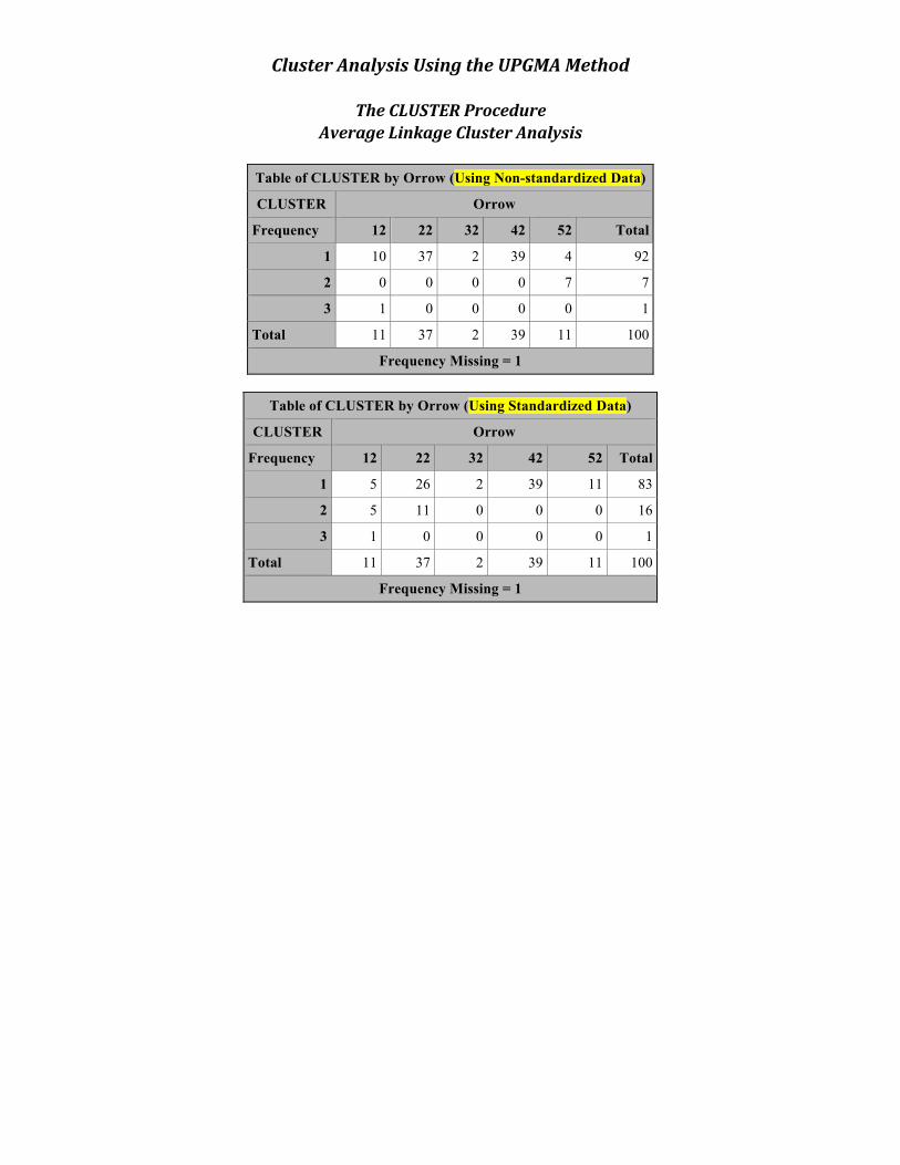
Table of CLUSTER by Orrow (Using Non-standardized Data)
CLUSTER Orrow
Frequency 12 22 32 42 52 Total
1 10 37 2 39 4 92
2 0 0 0 0 7 7
3 1 0 0 0 0 1
Total 11 37 2 39 11 100
Frequency Missing = 1
Table of CLUSTER by Orrow (Using Standardized Data)
CLUSTER Orrow
Frequency 12 22 32 42 52 Total
1 5 26 2 39 11 83
2 5 11 0 0 0 16
3 1 0 0 0 0 1
Total 11 37 2 39 11 100
Frequency Missing = 1

Cluster Analysis Using the UPGMA Method
The CLUSTER Procedure Average Linkage Cluster Analysis
Non-‐standardized Data

Cluster Analysis Using the UPGMA Method
The FREQ Procedure (Using Standardized Data)
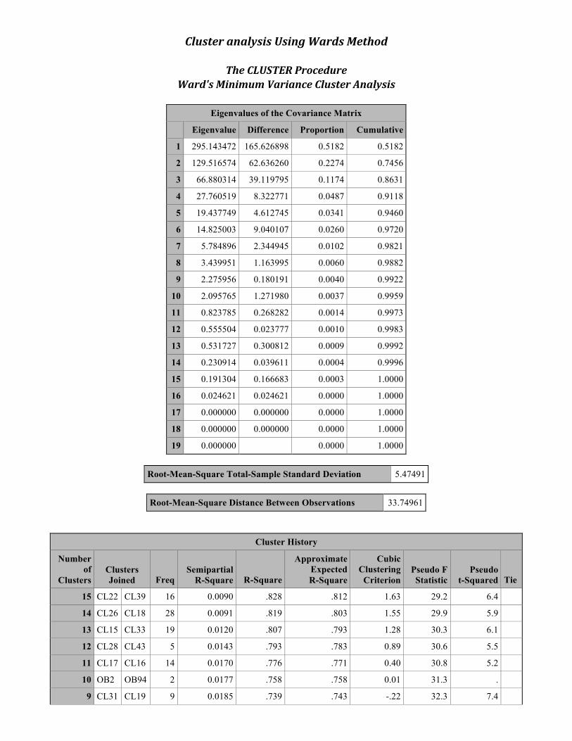
Cluster analysis Using Wards Method
The CLUSTER Procedure Ward's Minimum Variance Cluster Analysis
Eigenvalues of the Covariance Matrix
Eigenvalue Difference Proportion Cumulative
1 295.143472 165.626898 0.5182 0.5182
2 129.516574 62.636260 0.2274 0.7456
3 66.880314 39.119795 0.1174 0.8631
4 27.760519 8.322771 0.0487 0.9118
5 19.437749 4.612745 0.0341 0.9460
6 14.825003 9.040107 0.0260 0.9720
7 5.784896 2.344945 0.0102 0.9821
8 3.439951 1.163995 0.0060 0.9882
9 2.275956 0.180191 0.0040 0.9922
10 2.095765 1.271980 0.0037 0.9959
11 0.823785 0.268282 0.0014 0.9973
12 0.555504 0.023777 0.0010 0.9983
13 0.531727 0.300812 0.0009 0.9992
14 0.230914 0.039611 0.0004 0.9996
15 0.191304 0.166683 0.0003 1.0000
16 0.024621 0.024621 0.0000 1.0000
17 0.000000 0.000000 0.0000 1.0000
18 0.000000 0.000000 0.0000 1.0000
19 0.000000 0.0000 1.0000
Root-Mean-Square Total-Sample Standard Deviation 5.47491
Root-Mean-Square Distance Between Observations 33.74961
Cluster History
Number of
Clusters Clusters Joined Freq
Semipartial R-Square R-Square
Approximate Expected R-Square
Cubic Clustering
Criterion Pseudo F Statistic
Pseudo t-Squared Tie
15 CL22 CL39 16 0.0090 .828 .812 1.63 29.2 6.4
14 CL26 CL18 28 0.0091 .819 .803 1.55 29.9 5.9
13 CL15 CL33 19 0.0120 .807 .793 1.28 30.3 6.1
12 CL28 CL43 5 0.0143 .793 .783 0.89 30.6 5.5
11 CL17 CL16 14 0.0170 .776 .771 0.40 30.8 5.2
10 OB2 OB94 2 0.0177 .758 .758 0.01 31.3 .
9 CL31 CL19 9 0.0185 .739 .743 -.22 32.3 7.4
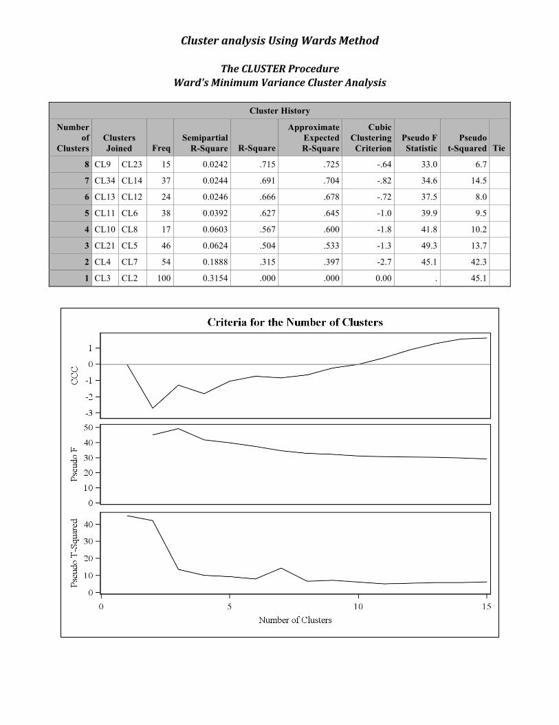
Cluster analysis Using Wards Method
The CLUSTER Procedure Ward's Minimum Variance Cluster Analysis
Cluster History
Number of
Clusters Clusters Joined Freq
Semipartial R-Square R-Square
Approximate Expected R-Square
Cubic Clustering
Criterion Pseudo F Statistic
Pseudo t-Squared Tie
8 CL9 CL23 15 0.0242 .715 .725 -.64 33.0 6.7
7 CL34 CL14 37 0.0244 .691 .704 -.82 34.6 14.5
6 CL13 CL12 24 0.0246 .666 .678 -.72 37.5 8.0
5 CL11 CL6 38 0.0392 .627 .645 -1.0 39.9 9.5
4 CL10 CL8 17 0.0603 .567 .600 -1.8 41.8 10.2
3 CL21 CL5 46 0.0624 .504 .533 -1.3 49.3 13.7
2 CL4 CL7 54 0.1888 .315 .397 -2.7 45.1 42.3
1 CL3 CL2 100 0.3154 .000 .000 0.00 . 45.1

Cluster analysis Using Wards Method
The CLUSTER Procedure Ward's Minimum Variance Cluster Analysis
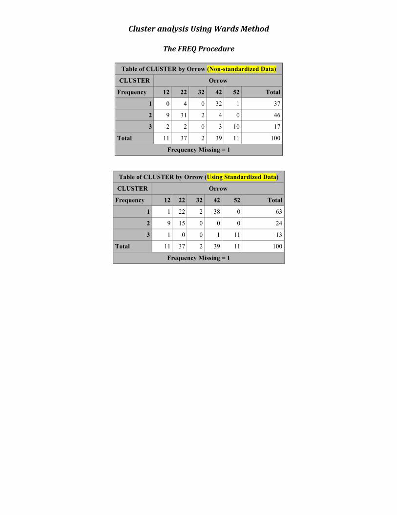
Cluster analysis Using Wards Method
The FREQ Procedure
Table of CLUSTER by Orrow (Non-standardized Data)
CLUSTER Orrow
Frequency 12 22 32 42 52 Total
1 0 4 0 32 1 37
2 9 31 2 4 0 46
3 2 2 0 3 10 17
Total 11 37 2 39 11 100
Frequency Missing = 1
Table of CLUSTER by Orrow (Using Standardized Data)
CLUSTER Orrow
Frequency 12 22 32 42 52 Total
1 1 22 2 38 0 63
2 9 15 0 0 0 24
3 1 0 0 1 11 13
Total 11 37 2 39 11 100
Frequency Missing = 1
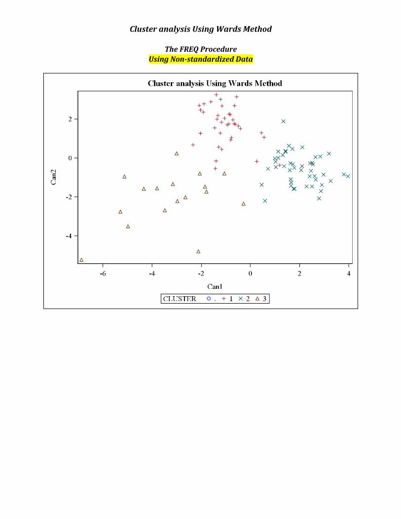
Cluster analysis Using Wards Method
The FREQ Procedure Using Non-‐standardized Data

Cluster analysis Using Wards Method
The FREQ Procedure Using Standardized Data