cluster failure: why fmri inferences for spatial extent...

Cluster failure: Why fMRI inferences for spatial extenthave inflated false-positive ratesAnders Eklunda,b,c,1, Thomas E. Nicholsd,e, and Hans Knutssona,c

aDivision of Medical Informatics, Department of Biomedical Engineering, Linköping University, S-581 85 Linköping, Sweden; bDivision of Statistics andMachine Learning, Department of Computer and Information Science, Linköping University, S-581 83 Linköping, Sweden; cCenter for Medical ImageScience and Visualization, Linköping University, S-581 83 Linköping, Sweden; dDepartment of Statistics, University of Warwick, Coventry CV4 7AL, UnitedKingdom; and eWMG, University of Warwick, Coventry CV4 7AL, United Kingdom

Edited by Emery N. Brown, Massachusetts General Hospital, Boston, MA, and approved May 17, 2016 (received for review February 12, 2016)

The most widely used task functional magnetic resonance imaging(fMRI) analyses use parametric statistical methods that depend on avariety of assumptions. In this work, we use real resting-state dataand a total of 3 million random task group analyses to computeempirical familywise error rates for the fMRI software packages SPM,FSL, and AFNI, as well as a nonparametric permutation method. For anominal familywise error rate of 5%, the parametric statisticalmethods are shown to be conservative for voxelwise inferenceand invalid for clusterwise inference. Our results suggest that theprincipal cause of the invalid cluster inferences is spatial autocorre-lation functions that do not follow the assumed Gaussian shape. Bycomparison, the nonparametric permutation test is found to producenominal results for voxelwise as well as clusterwise inference. Thesefindings speak to the need of validating the statistical methods beingused in the field of neuroimaging.

fMRI | statistics | false positives | cluster inference | permutation test

Since its beginning more than 20 years ago, functional magneticresonance imaging (fMRI) (1, 2) has become a popular tool

for understanding the human brain, with some 40,000 publishedpapers according to PubMed. Despite the popularity of fMRI as atool for studying brain function, the statistical methods used haverarely been validated using real data. Validations have insteadmainly been performed using simulated data (3), but it is obviouslyvery hard to simulate the complex spatiotemporal noise that arisesfrom a living human subject in an MR scanner.Through the introduction of international data-sharing initia-

tives in the neuroimaging field (4–10), it has become possible toevaluate the statistical methods using real data. Scarpazza et al.(11), for example, used freely available anatomical images from396 healthy controls (4) to investigate the validity of parametricstatistical methods for voxel-based morphometry (VBM) (12).Silver et al. (13) instead used image and genotype data from 181subjects in the Alzheimer’s Disease Neuroimaging Initiative(8, 9), to evaluate statistical methods common in imaging ge-netics. Another example of the use of open data is our previouswork (14), where a total of 1,484 resting-state fMRI datasets fromthe 1,000 Functional Connectomes Project (4) were used as nulldata for task-based, single-subject fMRI analyses with the SPMsoftware. That work found a high degree of false positives, up to70% compared with the expected 5%, likely due to a simplistictemporal autocorrelation model in SPM. It was, however, notclear whether these problems would propagate to group studies.Another unanswered question was the statistical validity of otherfMRI software packages. We address these limitations in thecurrent work with an evaluation of group inference with the threemost common fMRI software packages [SPM (15, 16), FSL (17),and AFNI (18)]. Specifically, we evaluate the packages in theirentirety, submitting the null data to the recommended suite ofpreprocessing steps integrated into each package.The main idea of this study is the same as in our previous one

(14). We analyze resting-state fMRI data with a putative taskdesign, generating results that should control the familywise error

(FWE), the chance of one or more false positives, and empiricallymeasure the FWE as the proportion of analyses that give rise toany significant results. Here, we consider both two-sample andone-sample designs. Because two groups of subjects are randomlydrawn from a large group of healthy controls, the null hypothesisof no group difference in brain activation should be true. More-over, because the resting-state fMRI data should contain noconsistent shifts in blood oxygen level-dependent (BOLD) activity,for a single group of subjects the null hypothesis of mean zeroactivation should also be true. We evaluate FWE control for bothvoxelwise inference, where significance is individually assessed ateach voxel, and clusterwise inference (19–21), where significanceis assessed on clusters formed with an arbitrary threshold.In brief, we find that all three packages have conservative

voxelwise inference and invalid clusterwise inference, for bothone- and two-sample t tests. Alarmingly, the parametric methodscan give a very high degree of false positives (up to 70%, com-pared with the nominal 5%) for clusterwise inference. By com-parison, the nonparametric permutation test (22–25) is found toproduce nominal results for both voxelwise and clusterwise in-ference for two-sample t tests, and nearly nominal results for one-sample t tests. We explore why the methods fail to appropriatelycontrol the false-positive risk.

ResultsA total of 2,880,000 random group analyses were performed tocompute the empirical false-positive rates of SPM, FSL, andAFNI; these comprise 1,000 one-sided random analyses repeatedfor 192 parameter combinations, three thresholding approaches,and five tools in the three software packages. The tested parameter

Significance

Functional MRI (fMRI) is 25 years old, yet surprisingly its mostcommon statistical methods have not been validated using realdata. Here, we used resting-state fMRI data from 499 healthycontrols to conduct 3 million task group analyses. Using this nulldata with different experimental designs, we estimate the in-cidence of significant results. In theory, we should find 5% falsepositives (for a significance threshold of 5%), but insteadwe foundthat the most common software packages for fMRI analysis (SPM,FSL, AFNI) can result in false-positive rates of up to 70%. Theseresults question the validity of some 40,000 fMRI studies and mayhave a large impact on the interpretation of neuroimaging results.

Author contributions: A.E. and T.E.N. designed research; A.E. and T.E.N. performed re-search; A.E., T.E.N., and H.K. analyzed data; and A.E., T.E.N., and H.K. wrote the paper.

The authors declare no conflict of interest.

This article is a PNAS Direct Submission.

Freely available online through the PNAS open access option.

See Commentary on page 7699.1To whom correspondence should be addressed. Email: [email protected].

This article contains supporting information online at www.pnas.org/lookup/suppl/doi:10.1073/pnas.1602413113/-/DCSupplemental.

7900–7905 | PNAS | July 12, 2016 | vol. 113 | no. 28 www.pnas.org/cgi/doi/10.1073/pnas.1602413113

http://crossmark.crossref.org/dialog/?doi=10.1073/pnas.1602413113&domain=pdf

mailto:[email protected]

http://www.pnas.org/lookup/suppl/doi:10.1073/pnas.1602413113/-/DCSupplemental

http://www.pnas.org/lookup/suppl/doi:10.1073/pnas.1602413113/-/DCSupplemental

www.pnas.org/cgi/doi/10.1073/pnas.1602413113

combinations, given in Table 1, are common in the fMRI fieldaccording to a recent review (26). The following five analysis toolswere tested: SPM OLS, FSL OLS, FSL FLAME1, AFNI OLS(3dttest++), and AFNI 3dMEMA. The ordinary least-squares (OLS)functions only use the parameter estimates of BOLD response mag-nitude from each subject in the group analysis, whereas FLAME1 inFSL and 3dMEMA in AFNI also consider the variance of the subject-specific parameter estimates. To compare the parametric statisticalmethods used by SPM, FSL, and AFNI to a nonparametric method,all analyses were also performed using a permutation test (22, 23, 27).All tools were used to generate inferences corrected for the FWE rateover the whole brain.Resting-state fMRI data from 499 healthy controls, down-

loaded from the 1,000 Functional Connectomes Project (4), wereused for all analyses. Resting-state data should not contain sys-tematic changes in brain activity, but our previous work (14)showed that the assumed activity paradigm can have a large

impact on the degree of false positives. Several different activityparadigms were therefore used, two block based (B1 and B2) andtwo event related (E1 and E2); see Table 1 for details.Fig. 1 presents the main findings of our study, summarized by

a common analysis setting of a one-sample t test with 20 subjectsand 6-mm smoothing [see SI Appendix, Figs. S1–S6 (20 subjects)and SI Appendix, Figs. S7–S12 (40 subjects) for the full results].In broad summary, parametric software’s FWE rates for clus-terwise inference far exceed their nominal 5% level, whereasparametric voxelwise inferences are valid but conservative, oftenfalling below 5%. Permutation false positives are controlled at anominal 5% for the two-sample t test, and close to nominal forthe one-sample t test. The impact of smoothing and cluster-defining threshold (CDT) was appreciable for the parametricmethods, with CDT P = 0.001 (SPM default) having much betterFWE control than CDT P = 0.01 [FSL default; AFNI does nothave a default setting, but P = 0.005 is most prevalent (21)].

Table 1. Parameters tested for the different fMRI software packages, giving a total of 192 (3 × 2 × 2 × 4 × 2 × 2)parameter combinations and three thresholding approaches

Parameter Values used

fMRI data Beijing (198 subjects), Cambridge (198 subjects), Oulu (103 subjects)Block activity paradigms B1 (10-s on off), B2 (30-s on off)Event activity paradigms E1 (2-s activation, 6-s rest), E2 (1- to 4-s activation, 3- to 6-s rest, randomized)Smoothing 4-, 6-, 8-, 10-mm FWHMAnalysis type One-sample t test (group activation), two-sample t test (group difference)No. of subjects 20, 40Inference level Voxel, clusterCDT P = 0.01 (z = 2.3), P = 0.001 (z = 3.1)

One thousand group analyses were performed for each parameter combination.

SPM FLAME1 FSL OLS 3dttest 3dMEMA Perm

Fam

ilyw

ise

erro

r ra

te (

%)

0

10

20

30

40

50

60

70

80Beijing, one sample t-test, 6 mm, CDT p = 0.01

B1 10 s on offB2 30 s on offE1 2 s eventsE2 randomized eventsExpected95% CI


Fam

ilyw

ise

erro

r ra

te (

%)

0

10

20

30

40

50

60

70

80Beijing, one sample t-test, 6 mm, CDT p = 0.001


Fam

ilyw

ise

erro

r ra

te (

%)

0

10

20

30

40

50

60

70

80Beijing, one sample t-test, 6 mm, voxel inference


Fam

ilyw

ise

erro

r ra

te (

%)

0

10

20

30

40

50

60

70

80Cambridge, one sample t-test, 6 mm, CDT p = 0.01

B1 10 s on offB2 30 s on offE1 2 s eventsE2 randomized eventsExpected95% CI


Fam

ilyw

ise

erro

r ra

te (

%)

0

10

20

30

40

50

60

70

80Cambridge, one sample t-test, 6 mm, CDT p = 0.001

A

B


Fam

ilyw

ise

erro

r ra

te (

%)

0

10

20

30

40

50

60

70

80Cambridge, one sample t-test, 6 mm, voxel inference

Fig. 1. Results for one-sample t test, showing estimated FWE rates for (A) Beijing and (B) Cambridge data analyzed with 6 mm of smoothing and fourdifferent activity paradigms (B1, B2, E1, and E2), for SPM, FSL, AFNI, and a permutation test. These results are for a group size of 20. The estimated FWE ratesare simply the number of analyses with any significant group activation divided by the number of analyses (1,000). From Left to Right: Cluster inference usinga cluster-defining threshold (CDT) of P = 0.01 and a FWE-corrected threshold of P = 0.05, cluster inference using a CDT of P = 0.001 and a FWE-correctedthreshold of P = 0.05, and voxel inference using a FWE-corrected threshold of P = 0.05. Note that the default CDT is P = 0.001 in SPM and P = 0.01 in FSL (AFNIdoes not have a default setting).

Eklund et al. PNAS | July 12, 2016 | vol. 113 | no. 28 | 7901

NEU

ROSC

IENCE

STATIST

ICS

SEECO

MMEN

TARY

http://www.pnas.org/lookup/suppl/doi:10.1073/pnas.1602413113/-/DCSupplemental/pnas.1602413113.sapp.pdf




Among the parametric software packages, FSL’s FLAME1clusterwise inference stood out as having much lower FWE, of-ten being valid (under 5%), but this comes at the expense ofhighly conservative voxelwise inference.We also examined an ad hoc but commonly used thresholding

approach, where a CDT of P = 0.001 (uncorrected for multiplecomparisons) is used together with an arbitrary cluster extentthreshold of 10 8-mm3 voxels (26, 28). We conducted an addi-tional 1,000 analyses repeated for four assumed activity paradigmsand the five different analysis tools (Fig. 2). Although no precisecontrol of false positives is assured, we found this makeshift in-ference method had FWE ranging 60–90% for all functions exceptFLAME1 in FSL. Put another way, this “P = 0.001 + 10 voxels”method has a FWE-corrected P value of 0.6–0.9. We now seek tounderstand the sources of these inaccuracies.

Comparison of Empirical and Theoretical Test Statistic Distributions.As a first step to understand the inaccuracies in the parametricmethods, the test statistic values (t or z scores, as generated byeach package) were compared with their theoretical null distri-butions. SI Appendix, Fig. S13, shows the histogram of all brainvoxels for 1,000 group analyses. The empirical and theoreticalnulls are well matched, except for FSL FLAME1, which haslower variance (σ̂2 = 0.67) than the theoretical null (σ2 = 1). This isthe proximal cause of the highly conservative results from FSLFLAME1. The mixed-effects variance is composed of intrasubjectand intersubject variance (σ2WTN , σ

2BTW , respectively), and although

other software packages do not separately estimate each, FLAME1estimates each and constrains σ2BTW to be positive. In these nulldata, the true effect in each subject is zero, and thus the trueσ2BTW = 0. Thus, unless FLAME1’s σ̂2BWT is correctly estimated tobe 0, it can only be positively biased, and in fact this point wasraised by the original authors (29).In an follow-up analysis on FSL FLAME1 (SI Appendix), we

conducted two-sample t tests on task fMRI data, randomlysplitting subjects into two groups. In this setting, the two-sample

null hypothesis was still true, but σ2BTW > 0. Here, we found clusterfalse-positive rates comparable to FSL OLS (44.8% for CDTP = 0.01 and 13.8% for CDT P = 0.001), supporting our con-jecture of zero between-subject variance as the cause ofFLAME1’s conservativeness on completely null resting data.

Spatial Autocorrelation Function of the Noise. SPM and FSL dependon Gaussian random-field theory (RFT) for FWE-corrected vox-elwise and clusterwise inference. However, RFT clusterwise in-ference depends on two additional assumptions. The firstassumption is that the spatial smoothness of the fMRI signal isconstant over the brain, and the second assumption is that thespatial autocorrelation function has a specific shape (a squaredexponential) (30). To investigate the second assumption, the spatialautocorrelation function was estimated and averaged using 1,000group difference maps. For each group difference map and eachdistance (1–20 mm), the spatial autocorrelation was estimated andaveraged along x, y, and z. The empirical spatial autocorrelationfunctions are given in SI Appendix, Fig. S14. A reference squaredexponential is also included for each software, based on an intrinsicsmoothness of 9.5 mm (FWHM) for SPM, 9 mm for FSL, and8 mm for AFNI (according to the mean smoothness of 1,000 groupanalyses, presented in SI Appendix, Fig. S15). The empirical spatialautocorrelation functions are clearly far from a squared exponen-tial, having heavier tails. This may explain why the parametricmethods work rather well for a high CDT (resulting in smallclusters, more reflective of local autocorrelation) and not as wellfor a low CDT (resulting in large clusters, reflecting distant auto-correlation). SI Appendix, Fig. S16, shows how the cluster extentthresholds differ between the parametric and the nonparametricmethods, for a CDT of P = 0.01. The nonparametric permutationtest is valid for any spatial autocorrelation function and finds muchmore stringent cluster extent thresholds (three to six times highercompared with SPM, FSL, and AFNI).To better understand the origin of the heavy tails, the spatial

autocorrelation was estimated at different preprocessing stages(no preprocessing, after motion correction, after motion correc-tion, and 6-mm smoothing) using the 198 subjects in the Beijingdataset. The resulting spatial autocorrelation functions are givenin SI Appendix, Fig. S17. It is clear that the long tails exist in theraw data and become even more pronounced after the spatialsmoothing. These long-tail spatial correlations also exist for MRphantoms (31) and can therefore be seen as scanner artifacts.

Spatial Distribution of False-Positive Clusters. To investigate whetherthe false clusters appear randomly in the brain, all significantclusters (P < 0.05, FWE-corrected) were saved as binary mapsand summed together (SI Appendix, Fig. S18). These maps ofvoxelwise cluster frequency show the areas more and less likelyto be marked as significant in a clusterwise analysis. Posteriorcingulate was the most likely area to be covered by a cluster,whereas white matter was least likely. As this distribution couldreflect variation in the local smoothness in the data, we usedgroup residuals from 1,000 two-sample t tests to estimate vox-elwise spatial smoothness (32) (SI Appendix, Fig. S19). Thelocal smoothness maps show evidence of a posterior cingulate“hot spot” and reduced intensity in white matter, just as in thefalse-positive cluster maps. Notably, having local smoothnessvarying systematically with tissue type has also been observedfor VBM data (13). In short, this suggests that violation of thestationary smoothness assumption may also be contributing tothe excess of false positives.In a follow-up analysis using the nonstationary toolbox for

SPM (fmri.wfubmc.edu/cms/software#NS), which providesparametric cluster inference allowing for spatially varyingsmoothness, we calculated FWE rates for stationary as well asnonstationary smoothness. Use of nonstationary cluster size in-ference did not produce nominal FWE: relative to the stationary

SPM FLAME1 FSL OLS 3dttest 3dMEMA

Fam

ilyw

ise

erro

r ra

te (

%)

0

10

20

30

40

50

60

70

80

90

100Beijing, two sample t-test, 6 mm, ad-hoc cluster inference

B1B2E1E2

Fig. 2. Results for two-sample t test and ad hoc clusterwise inference,showing estimated FWE rates for 6 mm of smoothing and four different ac-tivity paradigms (B1, B2, E1, and E2), for SPM, FSL, and AFNI. These results weregenerated using the Beijing data and 20 subjects in each group analysis. Eachstatistic map was first thresholded using a CDT of P = 0.001 (uncorrected formultiple comparisons), and the surviving clusters were then compared with acluster extent threshold of 80mm3 (10 voxels for SPM and FSL which used 2 × 2 ×2 mm3 voxels, three voxels for AFNI, which used 3 × 3 × 3 mm3 voxels). Theestimated FWE rates are simply the number of analyses with a significant resultdivided by the number of analyses (1,000).

7902 | www.pnas.org/cgi/doi/10.1073/pnas.1602413113 Eklund et al.









http://fmri.wfubmc.edu/cms/software#NS


cluster size test, it produced lower but still invalid FWE for aCDT of P = 0.01, and higher FWE for a CDT of P = 0.001 (SIAppendix, Table S2). This inconclusive performance can be at-tributed to additional assumptions and approximations introducedby the nonstationary cluster size test that can degrade its perfor-mance (33, 34). In short, we still cannot rule out heterogeneoussmoothness as contributor to the standard cluster size methods’invalid performance.

Impact on a Non-Null, Task Group Analysis. All of the analyses to thispoint have been based on resting-state fMRI data, where the nullhypothesis should be true. We now use task data to address thepractical question of “How will my FWE-corrected cluster Pvalues change?” if a user were to switch from a parametric to anonparametric method. We use four task datasets [rhyme judg-ment, mixed gambles (35), living–nonliving decision with plain ormirror-reversed text, word and object processing (36)] down-loaded from OpenfMRI (7). The datasets were analyzed using aparametric (the OLS option in FSL’s FEAT) and a non-parametric method (the randomise function in FSL) using asmoothing of 5-mm FWHM (default option in FSL). The onlydifference between these two methods is that FSL FEAT-OLSrelies on Gaussian RFT to calculate the corrected clusterP values, whereas randomise instead uses the data itself. Theresulting cluster P values are given in SI Appendix, Table S3 (CDTof P = 0.01) and SI Appendix, Tables S4 and S5 (CDT of P = 0.001).SI Appendix, Fig. S20, summarizes these results, plotting the ratioof FWE-corrected P values, nonparametric to parametric, againstcluster size. All nonparametric P values were larger than para-metric (ratio > 1). Although this could be taken as evidence of aconservative nonparametric procedure, the extensive simulationsshowing valid nonparametric and invalid parametric cluster sizeinference instead suggest inflated (biased) significance in theparametric inferences. For CDT P = 0.01, there were 23 clusters(in 11 contrasts) with FWE parametric P values significant at P =0.05 that were not significant by permutation. For CDT P = 0.001,there were 11 such clusters (in eight contrasts). If we assume thatthese mismatches represent false positives, then the empiricalFWE for these 18 contrasts considered is 11/18 = 61% for CDTP = 0.01 and 8/18 = 44% for CDT P = 0.001. These findings in-dicate that the problems exist also for task-based fMRI data, andnot only for resting-state data.

Permutation Test for One-Sample t Test. Although permutationtests have FWE within the expected bounds for all two-sampletest results, for one-sample tests they can exhibit conservative orinvalid behavior. As shown in SI Appendix, Figs. S3, S4, S9, andS10, the FWE can be as low as 0.8% or as high as 40%. The one-sample permutation FWE varies between site (Beijing, Cam-bridge, Oulu), but within each site shows a consistent patternbetween the two CDTs and even for voxelwise inference. Theone-sample permutation test comprises a sign flipping pro-cedure, justified by symmetrically distributed errors (22). Al-though the voxel-level test statistics appear symmetric and dofollow the expected parametric t distribution (SI Appendix, Fig.S13), the statistic values benefit from the central limit theoremand their symmetry does not imply symmetry of the data. Weconducted tests of the symmetry assumption on the data forblock design B1, a case suffering both spuriously low (Cam-bridge) and high (Beijing, Oulu) FWE (SI Appendix). We foundvery strong evidence of asymmetric errors, but with no consistentpattern of asymmetry; that is, some brain regions showed positiveskew and others showed negative skew.

DiscussionUsing mass empirical analyses with task-free fMRI data, we havefound that the parametric statistical methods used for groupfMRI analysis with the packages SPM, FSL, and AFNI can

produce FWE-corrected cluster P values that are erroneous, beingspuriously low and inflating statistical significance. This calls intoquestion the validity of countless published fMRI studies based onparametric clusterwise inference. It is important to stress that wehave focused on inferences corrected for multiple comparisons ineach group analysis, yet some 40% of a sample of 241 recent fMRIpapers did not report correcting for multiple comparisons (26),meaning that many group results in the fMRI literature suffereven worse false-positive rates than found here (37). According tothe same overview (26), the most common cluster extent thresholdused is 80 mm3 (10 voxels of size 2 × 2 × 2 mm), for which theFWE was estimated to be 60–90% (Fig. 2).Compared with our previous work (14), the results presented

here are more important for three reasons. First, the currentstudy considers group analyses, whereas our previous studylooked at single-subject analyses. Second, we here investigate thevalidity of the three most common fMRI software packages (26),whereas we only considered SPM in our previous study. Third,although we confirmed the expected finding of permutation’svalidity for two-sample t tests, we found that some settings weconsidered gave invalid FWE control for one-sample permuta-tion tests. We identified skewed data as a likely cause of this andidentified a simple test for detecting skew in the data. Usersshould consider testing for skew before applying a one-sample ttest, but it remains an important area for developing newmethods for one-sample analyses (see, e.g., ref. 38).

Why Is Clusterwise Inference More Problematic than Voxelwise? Ourprincipal finding is that the parametric statistical methods workwell, if conservatively, for voxelwise inference, but not for clus-terwise inference. We note that other authors have found RFTclusterwise inference to be invalid in certain settings under sta-tionarity (21, 30) and nonstationarity (13, 33). This present work,however, is the most comprehensive to explore the typical pa-rameters used in task fMRI for a variety of software tools. Ourresults are also corroborated by similar experiments for struc-tural brain analysis (VBM) (11–13, 39, 40), showing that cluster-based P values are more sensitive to the statistical assumptions.For voxelwise inference, our results are consistent with a pre-vious comparison between parametric and nonparametric methodsfor fMRI, showing that a nonparametric permutation test canresult in more lenient statistical thresholds while offering precisecontrol of false positives (13, 41).Both SPM and FSL rely on RFT to correct for multiple com-

parisons. For voxelwise inference, RFT is based on the assumptionthat the activity map is sufficiently smooth, and that the spatialautocorrelation function (SACF) is twice-differentiable at theorigin. For clusterwise inference, RFT additionally assumes aGaussian shape of the SACF (i.e., a squared exponential co-variance function), that the spatial smoothness is constant over thebrain, and that the CDT is sufficiently high. The 3dClustSimfunction in AFNI also assumes a constant spatial smoothness anda Gaussian form of the SACF (because a Gaussian smoothing isapplied to each generated noise volume). It makes no assumptionon the CDT and should be accurate for any chosen value. As theFWE rates are far above the expected 5% for clusterwise in-ference, but not for voxelwise inference, one or more of theGaussian SACF, the stationary SACF, or the sufficiently highCDT assumptions (for SPM and FSL) must be untenable.

Why Does AFNIs Monte Carlo Approach, Unreliant on RFT, NotPerform Better? As can be observed in SI Appendix, Figs. S2, S4,S8, and S10, AFNI’s FWE rates are excessive even for a CDT ofP = 0.001. There are two main factors that explain these results.First, AFNI estimates the spatial group smoothness differently

compared with SPM and FSL. AFNI averages smoothness estimatesfrom the first-level analysis, whereas SPM and FSL estimate thegroup smoothness using the group residuals from the general


NEU

ROSC

IENCE

STATIST

ICS

SEECO

MMEN

TARY













linear model (32). The group smoothness used by 3dClustSim mayfor this reason be too low (compared with SPM and FSL; SIAppendix, Fig. S15).Second, a 15-year-old bug was found in 3dClustSim while

testing the three software packages (the bug was fixed by the AFNIgroup as of May 2015, during preparation of this manuscript).The bug essentially reduced the size of the image searched forclusters, underestimating the severity of the multiplicity correc-tion and overestimating significance (i.e., 3dClustSim FWE Pvalues were too low).Together, the lower group smoothness and the bug in 3dClustSim

resulted in cluster extent thresholds that are much lower comparedwith SPM and FSL (SI Appendix, Fig. S16), which resulted in par-ticularly high FWE rates. We find this to be alarming, as 3dClust-Sim is one of the most popular choices for multiple-comparisonscorrection (26).We note that FWE rates are lower with the bug-fixed 3dClustSim

function. As an example, the updated function reduces the de-gree of false positives from 31.0% to 27.1% for a CDT of P =0.01, and from 11.5% to 8.6% for a CDT of P = 0.001 (theseresults are for two-sample t tests using the Beijing data, analyzedwith the E2 paradigm and 6-mm smoothing).

Suitability of Resting-State fMRI as Null Data for Task fMRI. Onepossible criticism of our work is that resting-state fMRI data donot truly compromise null data, as they may be affected by con-sistent trends or transients, for example, at the start of the session.However, if this were the case, the excess false positives wouldappear only in certain paradigms and, in particular, least likely inthe randomized event-related (E2) design. Rather, the inflatedfalse positives were observed across all experiment types withparametric cluster size inference, limiting the role of any suchsystematic effects. Additionally, one could argue that the spatialstructure of resting fMRI, the very covariance that gives rise to“resting-state networks,” is unrepresentative of task data and inflatesthe spatial autocorrelation functions and induces nonstationarity.We do not believe this is the case because it has been shown thatresting-state networks can be estimated from the residuals of taskdata (42), suggesting that resting data and task noise share similarproperties. We assessed this in our four task datasets, estimating thespatial autocorrelation of the group residuals (SI Appendix, Fig. S21)and found the same type of heavy-tailed behavior as in the restingdata. Furthermore, the same type of heavy-tail spatial autocorrela-tion has been observed for data collected with anMR phantom (31).Finally, another follow-up analysis on task data (see Comparison ofEmpirical and Theoretical Test Statistic Distributions and SI Appendix,Task-Based fMRI Data, Human Connectome Project, a two-sample ttest on a random split of a homogeneous group of subjects) foundinflated false-positive rates similar to the null data. Altogether, wefind that these findings support the appropriateness of resting dataas a suitable null for task fMRI.

The Future of fMRI. It is not feasible to redo 40,000 fMRI studies,and lamentable archiving and data-sharing practices mean mostcould not be reanalyzed either. Considering that it is now pos-sible to evaluate common statistical methods using real fMRIdata, the fMRI community should, in our opinion, focus onvalidation of existing methods. The main drawback of a per-mutation test is the increase in computational complexity, as thegroup analysis needs to be repeated 1,000–10,000 times. How-ever, this increased processing time is not a problem in practice,

as for typical sample sizes a desktop computer can run a per-mutation test for neuroimaging data in less than a minute (27,43). Although we note that metaanalysis can play an importantrole in teasing apart false-positive findings from consistent re-sults, that does not mitigate the need for accurate inferentialtools that give valid results for each and every study.Finally, we point out the key role that data sharing played in this

work and its impact in the future. Although our massive empiricalstudy depended on shared data, it is disappointing that almostnone of the published studies have shared their data, neither theoriginal data nor even the 3D statistical maps. As no analysismethod is perfect, and new problems and limitations will be cer-tainly found in the future, we commend all authors to at leastshare their statistical results [e.g., via NeuroVault.org (44)] andideally the full data [e.g., via OpenfMRI.org (7)]. Such shared dataprovide enormous opportunities for methodologists, but also theability to revisit results when methods improve years later.

Materials and MethodsOnly publicly shared anonymized fMRI data were used in this study. Datacollection at the respective sites was subject to their local ethics review boards,who approved the experiments and the dissemination of the anonymized data.For the 1,000 Functional Connectomes Project, collectionof the Cambridgedatawas approved by the Massachusetts General Hospital partners’ institutionalreview board (IRB); collection of the Beijing data was approved by the IRB ofState Key Laboratory for Cognitive Neuroscience and Learning, Beijing NormalUniversity; and collection of the Oulu data was approved by the ethics com-mittee of the Northern Ostrobothnian Hospital District. Dissemination of thedata was approved by the IRBs of New York University Langone MedicalCenter and New Jersey Medical School (4). The word and object processingexperiment (36) was approved by the Berkshire National Health Service Re-search Ethics Committee. The mixed-gambles experiment (35), the rhymejudgment experiment, and the living–nonliving experiments were approvedby the University of California, Los Angeles, IRB. All subjects gave informedwritten consent after the experimental procedures were explained.

The resting-state fMRI data from the 499 healthy controls were analyzed inSPM, FSL, and AFNI according to standard processing pipelines, and theanalyses were repeated for four levels of smoothing (4-, 6-, 8-, and 10-mmFWHM) and four task paradigms (B1, B2, E1, and E2). Random group analyseswere then performed using the parametric functions in the three softwares(SPM OLS, FLAME1, FSL OLS, 3dttest, 3dMEMA) as well as the nonparametricpermutation test. The degree of false positives was finally estimated as thenumber of group analyses with any significant result, divided by the numberof group analyses (1,000). All of the processing scripts are available at https://github.com/wanderine/ParametricMultisubjectfMRI.

ACKNOWLEDGMENTS. We thank Robert Cox, Stephen Smith, Mark Wool-rich, Karl Friston, and Guillaume Flandin, who gave us valuable feedback onthis work. This study would not be possible without the recent data-sharinginitiatives in the neuroimaging field. We therefore thank the NeuroimagingInformatics Tools and Resources Clearinghouse and all of the researcherswho have contributed with resting-state data to the 1,000 FunctionalConnectomes Project. Data were also provided by the Human ConnectomeProject, WU-Minn Consortium (principal investigators: David Van Essen andKamil Ugurbil; Grant 1U54MH091657) funded by the 16 NIH Institutes andCenters that support the NIH Blueprint for Neuroscience Research, and bythe McDonnell Center for Systems Neuroscience at Washington University.We also thank Russ Poldrack and his colleagues for starting the OpenfMRIProject (supported by National Science Foundation Grant OCI-1131441) andall of the researchers who have shared their task-based data. The NvidiaCorporation, which donated the Tesla K40 graphics card used to run all thepermutation tests, is also acknowledged. This research was supported by theNeuroeconomic Research Initiative at Linköping University, by Swedish Re-search Council Grant 2013-5229 (“Statistical Analysis of fMRI Data”), theInformation Technology for European Advancement 3 Project BENEFIT(better effectiveness and efficiency by measuring and modelling of interven-tional therapy), and the Wellcome Trust.

1. Ogawa S, et al. (1992) Intrinsic signal changes accompanying sensory stimulation:

Functional brain mapping with magnetic resonance imaging. Proc Natl Acad Sci USA

89(13):5951–5955.2. Logothetis NK (2008) What we can do and what we cannot do with fMRI. Nature

453(7197):869–878.3. Welvaert M, Rosseel Y (2014) A review of fMRI simulation studies. PLoS One 9(7):e101953.

4. Biswal BB, et al. (2010) Toward discovery science of human brain function. Proc Natl

Acad Sci USA 107(10):4734–4739.5. Van Essen DC, et al.; WU-Minn HCP Consortium (2013) The WU-Minn Human Con-

nectome Project: An overview. Neuroimage 80:62–79.6. Poldrack RA, Gorgolewski KJ (2014) Making big data open: Data sharing in neuro-

imaging. Nat Neurosci 17(11):1510–1517.

7904 | www.pnas.org/cgi/doi/10.1073/pnas.1602413113 Eklund et al.







http://NeuroVault.org

http://OpenfMRI.org

https://github.com/wanderine/ParametricMultisubjectfMRI

https://github.com/wanderine/ParametricMultisubjectfMRI


7. Poldrack RA, et al. (2013) Toward open sharing of task-based fMRI data: The Open-fMRI project. Front Neuroinform 7(12):12.

8. Mueller SG, et al. (2005) The Alzheimer’s disease neuroimaging initiative.Neuroimaging Clin N Am 15(4):869–877, xi–xii.

9. Jack CR, Jr, et al. (2008) The Alzheimer’s Disease Neuroimaging Initiative (ADNI): MRImethods. J Magn Reson Imaging 27(4):685–691.

10. Poline JB, et al. (2012) Data sharing in neuroimaging research. Front Neuroinform6(9):9.

11. Scarpazza C, Sartori G, De Simone MS, Mechelli A (2013) When the single mattersmore than the group: Very high false positive rates in single case voxel based mor-phometry. Neuroimage 70:175–188.

12. Ashburner J, Friston KJ (2000) Voxel-based morphometry—the methods. Neuroimage11(6 Pt 1):805–821.

13. Silver M, Montana G, Nichols TE; Alzheimer’s Disease Neuroimaging Initiative (2011)False positives in neuroimaging genetics using voxel-based morphometry data.Neuroimage 54(2):992–1000.

14. Eklund A, Andersson M, Josephson C, Johannesson M, Knutsson H (2012) Doesparametric fMRI analysis with SPM yield valid results? An empirical study of 1484 restdatasets. Neuroimage 61(3):565–578.

15. Friston K, Ashburner J, Kiebel S, Nichols T, Penny W (2007) Statistical ParametricMapping: The Analysis of Functional Brain Images (Elsevier/Academic, London).

16. Ashburner J (2012) SPM: A history. Neuroimage 62(2):791–800.17. Jenkinson M, Beckmann CF, Behrens TE, Woolrich MW, Smith SM (2012) FSL.

Neuroimage 62(2):782–790.18. Cox RW (1996) AFNI: Software for analysis and visualization of functional magnetic

resonance neuroimages. Comput Biomed Res 29(3):162–173.19. Friston KJ, Worsley KJ, Frackowiak RSJ, Mazziotta JC, Evans AC (1994) Assessing the

significance of focal activations using their spatial extent. Hum Brain Mapp 1(3):210–220.

20. Forman SD, et al. (1995) Improved assessment of significant activation in functionalmagnetic resonance imaging (fMRI): Use of a cluster-size threshold. Magn Reson Med33(5):636–647.

21. Woo CW, Krishnan A, Wager TD (2014) Cluster-extent based thresholding in fMRIanalyses: Pitfalls and recommendations. Neuroimage 91:412–419.

22. Nichols TE, Holmes AP (2002) Nonparametric permutation tests for functional neu-roimaging: A primer with examples. Hum Brain Mapp 15(1):1–25.

23. Winkler AM, Ridgway GR, Webster MA, Smith SM, Nichols TE (2014) Permutationinference for the general linear model. Neuroimage 92:381–397.

24. Brammer MJ, et al. (1997) Generic brain activation mapping in functional magneticresonance imaging: A nonparametric approach. Magn Reson Imaging 15(7):763–770.

25. Bullmore ET, et al. (1999) Global, voxel, and cluster tests, by theory and permutation,for a difference between two groups of structural MR images of the brain. IEEETransactions on Medical Imaging 18(1):32–42.

26. Carp J (2012) The secret lives of experiments: Methods reporting in the fMRI litera-ture. Neuroimage 63(1):289–300.

27. Eklund A, Dufort P, Villani M, Laconte S (2014) BROCCOLI: Software for fast fMRIanalysis on many-core CPUs and GPUs. Front Neuroinform 8:24.

28. Lieberman MD, Cunningham WA (2009) Type I and type II error concerns in fMRIresearch: Re-balancing the scale. Soc Cogn Affect Neurosci 4(4):423–428.

29. Woolrich MW, Behrens TE, Beckmann CF, Jenkinson M, Smith SM (2004) Multilevellinear modelling for FMRI group analysis using Bayesian inference. Neuroimage 21(4):1732–1747.

30. Hayasaka S, Nichols TE (2003) Validating cluster size inference: Random field andpermutation methods. Neuroimage 20(4):2343–2356.

31. Kriegeskorte N, et al. (2008) Artifactual time-course correlations in echo-planar fMRIwith implications for studies of brain function. Int J Imaging Syst Technol 18(5-6):345–349.

32. Kiebel SJ, Poline JB, Friston KJ, Holmes AP, Worsley KJ (1999) Robust smoothnessestimation in statistical parametric maps using standardized residuals from the gen-eral linear model. Neuroimage 10(6):756–766.

33. Hayasaka S, Phan KL, Liberzon I, Worsley KJ, Nichols TE (2004) Nonstationary cluster-size inference with random field and permutation methods. Neuroimage 22(2):676–687.

34. Salimi-Khorshidi G, Smith SM, Nichols TE (2011) Adjusting the effect of non-stationarity in cluster-based and TFCE inference. Neuroimage 54(3):2006–2019.

35. Tom SM, Fox CR, Trepel C, Poldrack RA (2007) The neural basis of loss aversion indecision-making under risk. Science 315(5811):515–518.

36. Duncan KJ, Pattamadilok C, Knierim I, Devlin JT (2009) Consistency and variability infunctional localisers. Neuroimage 46(4):1018–1026.

37. Ioannidis JP (2005) Why most published research findings are false. PLoS Med 2(8):e124.38. Pavlicová M, Cressie NA, Santner TJ (2006) Testing for activation in data from FMRI

experiments. J Data Sci 4(3):275–289.39. Scarpazza C, Tognin S, Frisciata S, Sartori G, Mechelli A (2015) False positive rates in

voxel-based morphometry studies of the human brain: Should we be worried?Neurosci Biobehav Rev 52:49–55.

40. Meyer-Lindenberg A, et al. (2008) False positives in imaging genetics. Neuroimage40(2):655–661.

41. Nichols T, Hayasaka S (2003) Controlling the familywise error rate in functionalneuroimaging: A comparative review. Stat Methods Med Res 12(5):419–446.

42. Fair DA, et al. (2007) A method for using blocked and event-related fMRI data tostudy “resting state” functional connectivity. Neuroimage 35(1):396–405.

43. Eklund A, Dufort P, Forsberg D, LaConte SM (2013) Medical image processing on theGPU—past, present and future. Med Image Anal 17(8):1073–1094.

44. Gorgolewski KJ, et al. (2016) NeuroVault.org: A repository for sharing unthresholdedstatistical maps, parcellations, and atlases of the human brain. Neuroimage 124(Pt B):1242–1244.


NEU

ROSC

IENCE

STATIST

ICS

SEECO

MMEN

TARY

Supporting Information Appendix

Cluster failure: Why fMRI inferences for spatial extent have inflated false positive rates

Anders Eklund, Thomas Nichols, Hans Knutsson

Methods

Resting state fMRI data

Resting state fMRI data from 499 healthy controls were downloaded from the 1000 functional connectomes project [1]

(http://fcon 1000.projects.nitrc.org/fcpClassic/FcpTable.html). The Beijing, Cambridge, and Oulu datasets were selected for

their large sample sizes (198, 198 and 103 subjects respectively) and their narrow age ranges (Beijing: 18 - 26 years, mean

21.16, SD 1.83, Cambridge: 18 - 30 years, mean 21.03, SD 2.31, Oulu: 20 - 23 years, mean 21.52, SD 0.57). For the Beijing

data, there are 76 male and 122 female subjects. For the Cambridge data, there are 75 male and 123 female subjects. For the

Oulu data, there are 37 male and 66 female subjects. Three Tesla (T) MR scanners were used for the Beijing as well as for the

Cambridge data, while a 1.5 T scanner was used for the Oulu data.

The Beijing data were collected with a repetition time (TR) of 2 seconds and consist of 225 time points per subject, 64 x 64

x 33 voxels of size 3.125 x 3.125 x 3.6 mm3. The Cambridge data were collected with a TR of 3 seconds and consist of 119

time points per subject, 72 x 72 x 47 voxels of size 3 x 3 x 3 mm3. The Oulu data were collected for with a TR of 1.8 seconds

and consist of 245 time points per subject, 64 x 64 x 28 voxels of size 4 x 4 x 4.4 mm. For each subject there is one T1-weighted

anatomical volume which can be used for normalization to a brain template. According to the motion plots from FSL, four Oulu

subjects moved slightly more than 1 mm in any direction. According to motion plots from AFNI, one Cambridge subject, three

Beijing subjects and eight Oulu subjects moved slightly more than 1 mm. The fMRI data have not been corrected for geometric

distortions, and no field maps are available for this purpose.

We randomly selected subsets of subjects for one sample t-tests (group activation) and two-sample t-tests (group difference).

Since the subjects were not performing any task and all are healthy and of similar age, the number of analyses with one or more

significant effects should follow the nominal rate (analyses were performed separately for Beijing, Cambridge and Oulu). The

same approach has previously been used to test the validity of parametric statistics for voxel based morphometry [2, 3].

Random group generation

Each random group was created by first applying a random permutation to a list containing all the 198, or 103, subject numbers.

To create two random groups of 20 subjects each, the first 20 permuted subject numbers were put into group 1, and the

following 20 permuted subject numbers were put into group 2. According to the n choose k formula n!k!(n−k)! it is possible to

create approximately 1.31 · 1042 such random group divisions (for n = 198 and k = 40). This collection of random analyses is

not independent, but the estimate of the familywise false positive rate is unbiased (as the expectation operator is additive under

dependence). A total of 1,000 random analyses were used to estimate the FWE (the same 1,000 analyses for all softwares and

all parameter combinations), for which the normal approximation of the Binomial 95% confidence interval is 3.65% - 6.35% for

a nominal FWE of 5%. Since the independence assumption of this normal approximation does not hold, we conducted Monte

Carlo simulations to assess its accuracy (see Supplementary Table 1).

Supplementary Table 1: Monte Carlo simulations on the accuracy of normal approximation for Binomial 95% confidenceintervals, to address the dependence in the 1,000 subgroups drawn from 103 or 198 subjects. Normally distributed noisevolumes (103 or 198 volumes, 60 x 60 x 60 voxels of size 2 x 2 x 2 mm, no mask) were generated and smoothed with 10mm FWHM, and random subsets of n = 20 or 40 volumes were drawn, 1,000 times, and used to construct one-sample t-tests.Inference was performed using cluster inference, with a CDT of p = 0.01 or 0.001, as well as voxel inference. This entireprocess was repeated 1,000 times. The voxel and cluster size FWE thresholds were determined from a separate Monte Carlosimulation (10,000 realizations). We found that results with more smoothing resulted in more inflated confidence intervals, andhence only show the worst case 10 mm FWHM results here.

Number of subjects Sample size Inference 95% CI103 20 Voxel 3.40% - 7.00%103 20 Cluster, CDT p = 0.001 3.00% - 7.80%103 20 Cluster, CDT p = 0.01 2.50% - 8.70%103 40 Voxel 2.40% - 9.30%103 40 Cluster, CDT p = 0.001 1.90% - 11.30%103 40 Cluster, CDT p = 0.01 1.50% - 13.50%198 20 Voxel 3.40% - 6.60%198 20 Cluster, CDT p = 0.001 3.20% - 6.80%198 20 Cluster, CDT p = 0.01 2.80% - 7.20%198 40 Voxel 3.10% - 6.90%198 40 Cluster, CDT p = 0.001 2.50% - 7.50%198 40 Cluster, CDT p = 0.01 2.00% - 8.00%

Code availability

Parametric group analyses were performed using SPM 8 (http://www.fil.ion.ucl.ac.uk/spm/software/spm8/),

FSL 5.0.7 (http://fsl.fmrib.ox.ac.uk/fsldownloads/) and AFNI (http://afni.nimh.nih.gov/afni/download/afni/releases, compiled

August 13 2014, version 2011 12 21 1014). FSL can perform non-parametric group analyses using the function randomise,

but we here used our BROCCOLI software [4] (https://github.com/wanderine/BROCCOLI) to lower the processing time. All the

processing scripts are freely available (https://github.com/wanderine/ParametricMultisubjectfMRI) to show all the processing

settings and to facilitate replication of the results. Since all the software packages and all the fMRI data are also freely available,

anyone can replicate the results in this paper.

First level analyses

A processing script was used for each software package to perform first level analyses for each subject, resulting in brain

activation maps in a standard brain space (Montreal Neurological Institute (MNI) for SPM and FSL, and Talairach for AFNI).

All first level analyses involved normalization to a brain template, motion correction and different amounts of smoothing (4, 6,

8 and 10 mm full width at half maximum). Slice timing correction was not performed, as the slice timing information is not

available for these fMRI datasets. A general linear model (GLM) was applied to the preprocessed fMRI data, using different

regressors for activity (B1, B2, E1, E2). The estimated head motion parameters were used as additional regressors in the design

matrix, for all packages, to further reduce effects of head motion.

First level analyses for SPM were performed using a Matlab batch script, closely following the SPM manual. The spatial

normalization was done as a two step procedure, where the mean fMRI volume was first aligned to the anatomical volume

(using the function ’Coregister’ with default settings). The anatomical volume was aligned to MNI space using the function

’Segment’ (with default settings), and the two transforms were finally combined to transform the fMRI data to MNI space

at 2 mm isotropic resolution (using the function ’Normalise: Write’). Spatial smoothing was finally applied to the spatially

normalized fMRI data. The first level models were then fit in the atlas space, i.e. not in the subject space.

For FSL, first level analyses were setup through the FEAT GUI. The spatial normalization to the brain template

(MNI152 T1 2mm brain.nii.gz) was performed as a two step linear registration using the function FLIRT (which is the default

option). One fMRI volume was aligned to the anatomical volume using the BBR (boundary based registration) option in FLIRT

(default). The anatomical volume was aligned to MNI space using a linear registration with 12 degrees of freedom (default),

and the two transforms were finally combined. The first level models were fit in the subject space (after spatial smoothing), and

the contrasts and their variances were then transformed to the atlas space.

First level analyses in AFNI were performed using the standardized processing script afni proc.py, which creates a tcsh

script which contains all the calls to different AFNI functions. The spatial normalization to Talairach space was performed as

a two step procedure. One fMRI volume was first linearly aligned to the anatomical volume, using the script align epi anat.py.

The anatomical volume was then linearly aligned to the brain template (TT N27+tlrc) using the script @auto tlrc. The trans-

formations from the spatial normalization and the motion correction were finally applied using a single interpolation, resulting

in normalized fMRI data in an isotropic resolution of 3 mm. Spatial smoothing was applied to the spatially normalized fMRI

data, and the first level models were then fit in the atlas space (i.e. not in the subject space).

Default drift modeling or highpass filtering options were used in each of SPM, FSL and AFNI. A discrete cosine transform

with cutoff of 128 seconds was used for SPM, while highpass filters with different cutoffs where used for FSL (20 seconds for

activity paradigm B1, 60 seconds for B2 and 100 seconds for E1 and E2), matching the defaults used by the FEAT GUI, and

AFNI’s Legende polynomial order is 4 and 3 for the Beijing and the Cambridge data, respectively (based on total scan duration).

Temporal correlations were further corrected for with a global AR(1) model in SPM, an arbitrary temporal autocorrelation

function regularized with a Tukey taper and adaptive spatial smoothing in FSL and a voxel-wise ARMA(1,1) model in AFNI.

Group analyses

A second processing script was used for each software package to perform random effect group analyses, using the results

from the first level analyses. For SPM, group analyses were only performed with the resulting beta weights from the first level

analyses, using ordinary least squares (OLS) regression over subjects. For FSL, group analyses were performed both using

FLAME1 (which is the default option) and OLS. The FLAME1 function uses both the beta weight and the corresponding

variance of each subject, subsequently estimating a between subject variance. For AFNI, group analyses were performed using

the functions 3dttest++ (OLS, using beta estimates from the function 3dDeconvolve which assumes independent errors) and

3dMEMA (which is similar to FLAME1 in FSL, using beta and variance estimates from the function 3dREMLfit which uses a

voxel-wise ARMA(1,1) model of the errors).

For the non-parametric analyses in BROCCOLI, first level results from FSL were used with OLS regression. A one-sample

permutation test on measures of change (i.e. BOLD contrast images) is conducted by randomly flipping the sign of each subject’s

data. Also known as the wild bootstrap, this is an exact test when the errors at each voxel are symmetrically distributed [5]. A

two-sample permutation test proceeds by randomly re-assigning group labels to subjects. Each non-parametric group analysis

was performed using 1,000 permutations or sign flips, a random sample of the millions of possible sign-flips and permutations.

For each permutation the maximal test statistic (voxel statistic or cluster size) over the brain is retained, creating the null

maximum distribution used for FWE inference.

Voxel-wise FWE-corrected p-values from SPM and FSL were obtained based on their respective implementations of random

field theory [6], while AFNI FWE p-values were obtained with a Bonferroni correction for the number of voxels (AFNI does

not provide any specific program for voxel-wise FWE p-values). For the non-parametric analyses, FWE-corrected p-values

were calculated as the proportion of the maximum statistic null distribution being as large or larger than a given statistic value.

Cluster-wise FWE-corrected p-values from SPM and FSL were likewise obtained based on their implementations of random

field theory [7]. AFNI estimates FWE p-values with a simulation based procedure, 3dClustSim [8]. SPM and FSL estimate

smoothness from the residuals of the group level analysis (used for both voxel-wise and cluster-wise inference), while AFNI

uses the average of the first level analyses’ smoothness estimates. For the non-parametric analyses, FWE-corrected p-values

were calculated as the proportion of the maximum cluster size null distribution being as large or larger than a given cluster’s

size.

Each group analysis was considered to give a significant result if any cluster or voxel had a FWE-corrected p-value p < 0.05.

Symmetry assumption for permutation based one-sample t-test

The permutation based one-sample t-test requires that the errors are symmetrically distributed. To investigate this assumption,

voxel-wise skewness s was estimated according to

s =1n

∑ni=1(xi − x̄)3(

1n−1

∑ni=1(xi − x̄)2

)3/2 , (1)

where n is the number of subjects in each group analysis and xi represents the first level activity estimate for subject i. For

each random group analysis a sign flipping test (with 100 sign flips) was used to calculate voxel-wise p-values of skewness.

The voxel-wise mean was removed prior to the sign flipping, and the maximum and minimum skewness values across the

entire brain were saved for each sign flip to form the maximum and minimum null distributions (required to calculate corrected

p-values).

Testing 100 random one-sample n = 20 group analyses for skew, the vast majority of analyses had evidence for both positive

and negative skew. For the Beijing datasets analyzed with paradigm B1, 82 analyses had 5% FWE-significant positive skew,

86 significant negative skew; for Cambridge B1, 91 analyses had significant negative skew, 72 significant positive skew; for

Oulu B1, 99 analyses had significant positive skew and 94 significant negative skew. A given voxel cannot be both positively

and negatively skewed, but rather these results show that both positively and negatively skewed voxels are prevalent in all three

datasets. Interestingly, the skewness varies both with the spatial location and the assumed activity paradigm.

Why is cluster-wise inference more problematic than voxelwise?

Supplementary Figure 14 shows that the SACFs are far from a squared exponential. The empirical SACFs are close to a squared

exponential for small distances, but the autocorrelation is higher than expected for large distances. This could be the reason

why the parametric methods work rather well for a high cluster defining threshold (p = 0.001), and not at all for a low threshold

(p = 0.01). A low threshold gives large clusters with a large radius, for which the tail of the SACF is quite important. For a high

threshold, resulting in rather small clusters with a small radius, the tail is not as important. Also, it could simply be that the

high-threshold assumption is not satisfied for a CDT of p = 0.01. Supplementary Figure 19 shows that the spatial smoothness

is not constant in the brain, but varies spatially. Note that the bright areas match the spatial distribution of false clusters in

Supplementary Figure 18; it is more likely to find a large cluster for a high smoothness. The permutation test does not assume

a specific shape of the SACF, nor does it assume a constant spatial smoothness, nor require a high CDT. For these reasons, the

permutation test provides valid results, for two sample t-tests, for both voxel and cluster-wise inference.

Which parameters affect the familywise error rate for cluster-wise inference?

The cluster defining threshold is the most important parameter for SPM, FSL and AFNI; using a more liberal threshold increases

the degree of false positives. This result is consistent with previous work [9, 10, 11]. However, the permutation test is completely

unaffected by changes of this parameter. According to a recent review looking at 484 fMRI studies [10], the CDT used varies

greatly between the three software packages (mainly due to different default settings). SPM and FSL have default thresholds of

p = 0.001 and p = 0.01, respectively; while AFNI has no default setting, p = 0.005 is most prevalent.

The amount of smoothing has a rather large impact on the degree of false positives, especially for FSL OLS. The results

from the permutation test, on the other hand, do not depend on this parameter. The original fMRI data has an intrinsic SACF,

which is combined with the SACF of the smoothing kernel. The final SACF will more closely resemble a squared exponential

for high levels of smoothing, simply because the smoothing operation forces the data to have a more Gaussian SACF. The

permutation test does not assume a specific form of the SACF, and therefore performs well for any degree of smoothing.

All software packages are affected by the analysis type; the familywise error rates are generally lower for a two-sample

t-test compared to a one sample t-test. This is a reflection of the greater robustness of the two-sample t-test: a difference of two

variables (following the same distribution) has a symmetric distribution, which is an important facet of a normal distribution.

Task based fMRI data

OpenfMRI

Task based fMRI data were downloaded from the OpenfMRI project [12] (http://openfmri.org), to investigate how cluster based

p-values differ between parametric and non-parametric group analyses. Each task dataset contains fMRI data, anatomical data

and timing information for each subject. The datasets were only analyzed with FSL, using 5 mm of smoothing (the default

option). Motion regressors were used in all cases, to further suppress effects of head motion. Group analyses were performed

using the parametric OLS option (i.e. not the default FLAME1 option) and the non-parametric randomise function (which

performs OLS regression in each permutation).

Rhyme judgment

The rhyme judgment dataset is available at http://openfmri.org/dataset/ds000003. The 13 subjects (8 male, age range 18 - 38

years, mean 24.08, SD 6.52) were presented with pairs of either words or pseudo words and made rhyming judgments for each

pair. The design contains four 20 second blocks per category, with eight 2 second events in each block (each block is separated

with 20 seconds of rest). The fMRI data were collected with a repetition time of 2 seconds and consist of 160 time points per

subject, the spatial resolution is 3.125 x 3.125 x 4 mm3 (resulting in volumes of 64 x 64 x 33 voxels). The data were analyzed

with two regressors; one for words and one for pseudo words. A total of four contrasts were applied; words, pseudowords,

words - pseudo words, pseudo words - words. For a cluster defining threshold of p = 0.01, a t-threshold of 2.65 was used. For a

cluster defining threshold of p = 0.001, a t-threshold of 3.95 was used.

Mixed-gambles task

The mixed-gambles task dataset is available at http://openfmri.org/dataset/ds000005. The 16 subjects (8 male, age range 19 -

28 years, mean 22.06, SD 2.86) were presented with mixed (gain/loss) gambles, in an event related design, and decided whether

they would accept each gamble. No outcomes of these gambles were presented during scanning, but after the scan three gambles

were selected at random and played for real money. The fMRI data were collected using a 3 T Siemens Allegra scanner. A

repetition time of 2 seconds was used and a total of 240 volumes were collected for each run, the spatial resolution is 3.125

x 3.125 x 4 mm3 (resulting in volumes of 64 x 64 x 34 voxels). The dataset contains three runs per subject, but only the first

run was used in our analysis. The data were analyzed using four regressors; task, parametric gain, parametric loss and distance

from indifference. A total of four contrasts were applied; parametric gain, - parametric gain, parametric loss, - parametric loss.

For a cluster defining threshold of p = 0.01, a t-threshold of 2.57 was used. For a cluster defining threshold of p = 0.001, a

t-threshold of 3.75 was used.

Living-nonliving decision with plain or mirror-reversed text

The living-nonliving decision task dataset is available at http://openfmri.org/dataset/ds000006a. The 14 subjects (5 male, age

range 19 - 35 years, mean 22.79, SD 4.00) made living-nonliving decisions, in an event related design, on items presented in

either plain or mirror-reversed text. The fMRI data were collected using a 3 T Siemens Allegra scanner. A repetition time

of 2 seconds was used and a total of 205 volumes were collected for each run, the spatial resolution is 3.125 x 3.125 x 5

mm3 (resulting in volumes of 64 x 64 x 25 voxels). The dataset contains six runs per subject, but only the first run was used

in our analysis. The data were analyzed using five regressors; mirror-switched, mirror-nonswitched, plain-switched, plain-

nonswitched and junk. A total of four contrasts were applied; mirrored versus plain (1,1,-1,-1,0), switched versus non-switched

(1,-1,1,-1,0), switched versus non-switched mirrored only (1,-1,0,0,0) and switched versus non-switched plain only (0,0,1,-1,0).

For a cluster defining threshold of p = 0.01, a t-threshold of 2.615 was used. For a cluster defining threshold of p = 0.001, a

t-threshold of = 3.87 was used.

Word and object processing

The word and object processing task dataset is available at http://openfmri.org/dataset/ds000107. The 49 subjects (age range 19

- 38 years, mean 25) performed a visual one-back task with four categories of items: written words, objects, scrambled objects

and consonant letter strings. The design contains six 15 second blocks per category, with 16 fast events in each block. The

fMRI data were collected using a 1.5 T Siemens scanner. A repetition time of 3 seconds was used and a total of 165 volumes

were collected for each run, the spatial resolution is 3 x 3 x 3 mm3 (resulting in volumes of 64 x 64 x 35 voxels). The dataset

contains two runs per subject, but only the first run was used in our analysis. The data were analyzed using four regressors;

words, objects, scrambled objects, consonant strings. A total of six contrasts were applied; words, objects, scrambled objects,

consonant strings, objects versus scrambled objects (0,1,-1,0) and words versus consonant strings (1,0,0,-1). For a cluster

defining threshold of p = 0.01, a t-threshold of 2.38 was used. For a cluster defining threshold of p = 0.001, a t-threshold of 3.28

was used.

Human connectome project

We undertook a follow-up study to understand the conservative results in FSL’s FLAME1. FLAME1 estimates the between-

subject variance as a positive quantity; while this is natural, if the true between-subject variance is zero, an imperfect (i.e.

non-zero) estimation will induce a positive bias and attenuate Z values. The resting fMRI data should have between-subject

variance of zero, while task data usually would have a non-zero between-subject variance. To assess FLAME1 under more

typical but still null settings, we created randomized two-group studies on task fMRI data; a homogeneous group of subjects

were split into two equal groups, meaning that the null of equal group activation is true, but there is activation present in the

data and likely appreciable between-subject variance.

Specifically, task based fMRI data were downloaded from the human connectome project

(HCP, http://www.humanconnectome.org/, ”Unrelated 80”), to investigate the degree of false positives using task data. fMRI

data from 80 unrelated healthy subjects (36 male, age range 22 - 36 years) were downloaded. A total of 7 task datasets

were used for all subjects (working memory, gambling, motor, language, social cognition, relational processing, emotion pro-

cessing), resulting in a total of 87 task contrasts. The fMRI data were collected using a 3 T Siemens Connectome Skyra

scanner, with a multiband gradient echo EPI sequence. A repetition time of 0.72 seconds was used, and the spatial resolu-

tion is 2 x 2 x 2 mm3 (resulting in volumes of 104 x 90 x 72 voxels). See the HCP website for information about the tasks;

http://www.humanconnectome.org/documentation/Q1/task-fMRI-protocol-details.html.

For each of the 87 contrasts, a two sample t-test was applied to a random split of the 80 subjects into two groups of 40

subjects. Each contrast resulting in a significant group difference (p < 0.05, FWE cluster corrected) was then counted as a false

positive.

(a) (b)

(c)

Supplementary Figure 1: Results for two sample t-test and cluster-wise inference using a cluster defining threshold (CDT) ofp = 0.01, showing estimated familywise error rates for 4 - 10 mm of smoothing and four different activity paradigms (B1, B2,E1, E2), for SPM, FSL, AFNI and a permutation test. These results are for a group size of 10 (giving a total of 20 subjects).Each statistic map was first thresholded using a CDT of p = 0.01, uncorrected for multiple comparisons, and the survivingclusters were then compared to a FWE-corrected cluster extent threshold, pFWE = 0.05. The estimated familywise error ratesare simply the number of analyses with any significant group differences divided by the number of analyses (1,000). Note thatthe default CDT is p = 0.001 in SPM and p = 0.01 in FSL (AFNI does not have a default setting). Also note that the defaultamount of smoothing is 8 mm in SPM, 5 mm in FSL and 4 mm in AFNI. (a) results for Beijing data (b) results for Cambridgedata (c) results for Oulu data.

(a) (b)

(c)


(a) (b)

(c)

Supplementary Figure 3: Results for one sample t-test and cluster-wise inference using a cluster defining threshold (CDT) ofp = 0.01, showing estimated familywise error rates for 4 - 10 mm of smoothing and four different activity paradigms (B1, B2,E1, E2), for SPM, FSL, AFNI and a permutation test. These results are for a group size of 20. Each statistic map was firstthresholded using a CDT of p = 0.01, uncorrected for multiple comparisons, and the surviving clusters were then comparedto a FWE-corrected cluster extent threshold, pFWE = 0.05. The estimated familywise error rates are simply the number ofanalyses with any significant group activations divided by the number of analyses (1,000). Note that the default CDT is p =0.001 in SPM and p = 0.01 in FSL (AFNI does not have a default setting). Also note that the default amount of smoothing is8 mm in SPM, 5 mm in FSL and 4 mm in AFNI. (a) results for Beijing data (b) results for Cambridge data (c) results for Ouludata.

(a) (b)

(c)

Supplementary Figure 4: Results for one sample t-test and cluster-wise inference using a cluster defining threshold (CDT)of p = 0.001, showing estimated familywise error rates for 4 - 10 mm of smoothing and four different activity paradigms (B1,B2, E1, E2), for SPM, FSL, AFNI and a permutation test. These results are for a group size of 20. Each statistic map was firstthresholded using a CDT of p = 0.001, uncorrected for multiple comparisons, and the surviving clusters were then comparedto a FWE-corrected cluster extent threshold, pFWE = 0.05. The estimated familywise error rates are simply the number ofanalyses with any significant group activations divided by the number of analyses (1,000). Note that the default CDT is p =0.001 in SPM and p = 0.01 in FSL (AFNI does not have a default setting). Also note that the default amount of smoothing is8 mm in SPM, 5 mm in FSL and 4 mm in AFNI. (a) results for Beijing data (b) results for Cambridge data (c) results for Ouludata.

(a) (b)

(c)

Supplementary Figure 5: Results for two-sample t-test and voxel-wise inference, showing estimated familywise error ratesfor 4 - 10 mm of smoothing and four different activity paradigms (B1, B2, E1, E2), for SPM, FSL, AFNI and a permutationtest. These results are for a group size of 10 (giving a total of 20 subjects). Each statistic map was thresholded using a FWE-corrected voxel-wise threshold of pFWE = 0.05. The estimated familywise error rates are simply the number of analyses withany significant results divided by the number of analyses (1,000). Note that the default amount of smoothing is 8 mm in SPM, 5mm in FSL and 4 mm in AFNI. (a) results for Beijing data (b) results for Cambridge data (c) results for Oulu data.

(a) (b)

(c)

Supplementary Figure 6: Results for one-sample t-test and voxel-wise inference, showing estimated familywise error rates for4 - 10 mm of smoothing and four different activity paradigms (B1, B2, E1, E2), for SPM, FSL, AFNI and a permutation test.These results are for a group size of 20. Each statistic map was thresholded using a FWE-corrected voxel-wise threshold ofpFWE = 0.05. The estimated familywise error rates are simply the number of analyses with any significant results divided bythe number of analyses (1,000). Note that the default amount of smoothing is 8 mm in SPM, 5 mm in FSL and 4 mm in AFNI.(a) results for Beijing data (b) results for Cambridge data (c) results for Oulu data.

(a) (b)

(c)


(a) (b)

(c)

Supplementary Figure 9: Results for one sample t-test and cluster-wise inference using a cluster defining threshold (CDT) ofp = 0.01, showing estimated familywise error rates for 4 - 10 mm of smoothing and four different activity paradigms (B1, B2,E1, E2), for SPM, FSL, AFNI and a permutation test. These results are for a group size of 40. Each statistic map was firstthresholded using a CDT of p = 0.01, uncorrected for multiple comparisons, and the surviving clusters were then comparedto a FWE-corrected cluster extent threshold, pFWE = 0.05. The estimated familywise error rates are simply the number ofanalyses with any significant group activations divided by the number of analyses (1,000). Note that the default CDT is p =0.001 in SPM and p = 0.01 in FSL (AFNI does not have a default setting). Also note that the default amount of smoothing is8 mm in SPM, 5 mm in FSL and 4 mm in AFNI. (a) results for Beijing data (b) results for Cambridge data (c) results for Ouludata.

(a) (b)

(c)

Supplementary Figure 10: Results for one sample t-test and cluster-wise inference using a cluster defining threshold (CDT)of p = 0.001, showing estimated familywise error rates for 4 - 10 mm of smoothing and four different activity paradigms (B1,B2, E1, E2), for SPM, FSL, AFNI and a permutation test. These results are for a group size of 40. Each statistic map was firstthresholded using a CDT of p = 0.001, uncorrected for multiple comparisons, and the surviving clusters were then comparedto a FWE-corrected cluster extent threshold, pFWE = 0.05. The estimated familywise error rates are simply the number ofanalyses with any significant group activations divided by the number of analyses (1,000). Note that the default CDT is p =0.001 in SPM and p = 0.01 in FSL (AFNI does not have a default setting). Also note that the default amount of smoothing is8 mm in SPM, 5 mm in FSL and 4 mm in AFNI. (a) results for Beijing data (b) results for Cambridge data (c) results for Ouludata.

(a) (b)

(c)

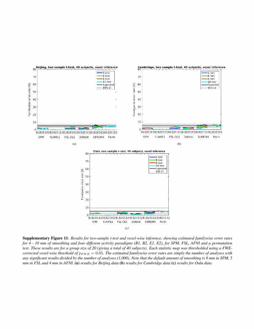
Supplementary Figure 11: Results for two-sample t-test and voxel-wise inference, showing estimated familywise error ratesfor 4 - 10 mm of smoothing and four different activity paradigms (B1, B2, E1, E2), for SPM, FSL, AFNI and a permutationtest. These results are for a group size of 20 (giving a total of 40 subjects). Each statistic map was thresholded using a FWE-corrected voxel-wise threshold of pFWE = 0.05. The estimated familywise error rates are simply the number of analyses withany significant results divided by the number of analyses (1,000). Note that the default amount of smoothing is 8 mm in SPM, 5mm in FSL and 4 mm in AFNI. (a) results for Beijing data (b) results for Cambridge data (c) results for Oulu data.

(a) (b)

(c)

Supplementary Figure 12: Results for one-sample t-test and voxel-wise inference, showing estimated familywise error ratesfor 4 - 10 mm of smoothing and four different activity paradigms (B1, B2, E1, E2), for SPM, FSL, AFNI and a permutation test.These results are for a group size of 40. Each statistic map was thresholded using a FWE-corrected voxel-wise threshold ofpFWE = 0.05. The estimated familywise error rates are simply the number of analyses with any significant results divided bythe number of analyses (1,000). Note that the default amount of smoothing is 8 mm in SPM, 5 mm in FSL and 4 mm in AFNI.(a) results for Beijing data (b) results for Cambridge data (c) results for Oulu data.

(a)

(b)

(c)

Supplementary Figure 13: Empirical versus theoretical null distributions for a) SPM, b) FSL and c) AFNI. The empiricalnull distributions were estimated by pooling test values over all brain voxels for 1,000 random group comparisons. The testvalues were drawn from two sample t-tests (10 subjects per group) using the Beijing data (analyzed with the E2 paradigm and6 mm smoothing). Note that the empirical null distribution for FLAME1 in FSL has a much lower variance (0.67) comparedto a normal distribution with unit variance. For this reason, the familywise error rates are much lower for FLAME in FSL,compared to the other functions.

(a)

(b)

(c)

Supplementary Figure 14: Empirical versus theoretical spatial autocorrelation functions (SACFs) for a) SPM, b) FSL andc) AFNI. The SACFs were estimated and averaged using 1,000 group difference maps, generated from two sample t-tests (10subjects per group) using the Beijing data (analyzed with the E2 paradigm and 6 mm smoothing). Note that the empiricalSACFs have a much longer tail compared to the theoretical squared exponential SACF, thereby violating one of the requiredassumptions for parametric cluster-wise inference using Gaussian random field theory. Both SPM and FSL resample the fMRIdata to a resolution of 2 mm, while AFNI instead uses a resolution of 3 mm for the specific datasets. For this reason, the SACFsare sampled differently for AFNI.

Supplementary Figure 15: Group smoothness estimates (mm full width at half maximum) for SPM, FSL FLAME and AFNI.The smoothness estimates originate from 1,000 two sample t-tests (10 subjects per group) using the Beijing data (analyzed withthe E2 paradigm and 6 mm smoothing). Note that AFNI estimates the group smoothness differently compared to SPM and FSL.Also note that AFNI uses higher order interpolation for motion correction and spatial normalization, which leads to a lowersmoothness compared to more common linear interpolation. The error bars represent the standard deviation.

Supplementary Figure 16: Cluster extent thresholds (in cubic millimeters) for SPM, FSL FLAME, AFNI and a permutationtest, for a cluster defining threshold of p = 0.01 and a familywise cluster error rate of p = 0.05. The thresholds originate from1,000 two sample t-tests (10 subjects per group) using the Beijing data (analyzed with the E2 paradigm and 6 mm smoothing).Note that the permutation threshold can only be directly compared with the threshold from the FSL software, as first level resultsfrom FSL were used for the non-parametric analyses. The error bars represent the standard deviation.

Supplementary Figure 17: Spatial autocorrelation functions (SACFs) for raw fMRI data, fMRI data after motion correctionand fMRI data after motion correction and 6 mm smoothing. A theoretical squared exponential is included as reference. TheSACFs were estimated and averaged using the 198 subjects in the Beijing dataset. Note that the long tail exists for the SACFof the raw data. These long tails have also been observed in data collected with an MR phantom [13], indicating that it is ascanner artifact.

(a)

(b)

(c)

Supplementary Figure 18: The maps show voxel-wise incidence of false clusters. Image intensity is the number of times, outof 10,000 random analyses (200,000 for FSL FLAME, to account for fewer clusters per analysis), a significant cluster occurredat a given voxel (CDT p = 0.01), for a) SPM, b) FSL and c) AFNI. Each analysis is a two sample t-test (10 subjects pergroup) using the Beijing data, analyzed with the E2 paradigm and 6 mm smoothing. The bright spot in the posterior cingulatecorresponds to a region of high smoothness, and suggests non-stationarity as a possible contributing factor.

(a)

(b)

(c)

Supplementary Figure 19: Maps of voxel-wise smoothness for a) SPM, b) FSL and c) AFNI. The smoothness was estimatedand averaged using 1,000 group residuals, generated from two sample t-tests (10 subjects per group) using the Beijing data(analyzed with the E2 paradigm and 6 mm smoothing). It is clear that the smoothness varies spatially; one of the requiredassumptions for parametric cluster-wise inference using Gaussian random field theory is thereby violated. Note that the brightareas (high smoothness) match the spatial maps of the false clusters; it is more likely to find a large cluster for areas with a highsmoothness. Note the reduced smoothness for the iterative method AFNI 3dMEMA compared to the corresponding non-iterativemethod AFNI OLS; the voxel-by-voxel estimation of between subject variance in the iterative methods reduces the smoothnessslightly.

Supplementary Figure 20: Ratio of non-parametric to parametric FWE corrected p-values for cluster size inference on 4 task(non-null) fMRI datasets, for parametric FWE p-values 0.05 ≥ p ≥ 10−4. Results for two CDT are shown, p = 0.01 and p =0.001, and larger ratios indicate parametric p-values being smaller (more significant) than non-parametric p-values (note thelogarithmic scale on the y-axis). Clusters with a parametric FWE p-value more significant than 10−4 are excluded because apermutation test with 5000 permutations can only resolve p-values down to 0.0002, and such p-values would generate largeratios inherently. These results suggest cluster size inference with a CDT of p = 0.01 has FWE inflated by 2 to almost 3 ordersof magnitude, and a CDT of p = 0.001 has FWE significance inflated by up to 2 orders of magnitude.

(a) (b)

(c) (d)

Supplementary Figure 21: Empirical versus theoretical spatial autocorrelation functions (SACFs) for the four task datasets; a)mixed-gambles b) rhyme judgment c) living-nonliving decision with plain or mirror-reversed text d) word and object processing.The SACFs were estimated using the group residuals from each group analysis. The fMRI data for each subject were analyzedin FSL, using 5 mm of smoothing (FSL default). Note that the empirical SACFs have a much longer tail compared to thetheoretical squared exponential SACF, thereby violating one of the required assumptions for parametric cluster-wise inferenceusing Gaussian random field theory.

Supplementary Table 2: Estimated familywise error rates (FWE) for parametric stationary and non-stationary cluster infer-ence. The results are for a two-sample t-test, 10 subjects per group, for data analayzed with the B2 paradigm and 4 mmsmoothing.

Dataset Cluster defining threshold Stationary FWE Non-stationary FWEBeijing p = 0.01 21.8% 15.8%Beijing p = 0.001 7.6% 10.9%

Cambridge p = 0.01 23.8% 17.6%Cambridge p = 0.001 7.9% 10.9%

Oulu p = 0.01 15.5% 12.5%Oulu p = 0.001 6.3% 13.4%

Supplementary Table 3: Cluster FWE p-values for FSL OLS and a permutation test, for 4 fMRI studies comprising a total of18 contrasts. A cluster defining threshold of p = 0.01 (z = 2.3) was used, all clusters with FSL OLS FWE p < 0.05 are listed. Astar denotes that the parametric p-value is below 0.05, while the non-parametric p-value is not. Note that the resolution of thepermutation p-values is 0.0002, since 5000 permutations (or sign flips) were used.

OpenfMRI dataset Subjects Cluster size (voxels) FSL OLS p-value Perm OLS p-valueRhyme judgment, contrast 1 13 53877 0 0.0002Rhyme judgment, contrast 2 13 27484 0 0.0002

14682 1.37 · 10−40 0.0023467 1.16 · 10−14 0.024

Rhyme judgment, contrast 3 13 799 4.8 · 10−5 0.097 *408 0.0103 0.219 *

Rhyme judgment, contrast 4 13 No surviving clustersMixed gambles, contrast 1 16 13284 1.36 · 10−36 0.005

440 0.0152 0.202 *Mixed gambles, contrast 2 16 No surviving clustersMixed gambles, contrast 3 16 No surviving clustersMixed gambles, contrast 4 16 655 0.00888 0.118 *

Living-nonliving decision, contrast 1 14 8612 3.46 · 10−33 0.0017577 2.37 · 10−30 0.0025920 1.6 · 10−25 0.0031439 4.88 · 10−9 0.035601 0.000213 0.116 *

Living-nonliving decision, contrast 2 14 751 2.75 · 10−5 0.08 *669 8.71 · 10−5 0.096 *546 0.000541 0.128 *

Living-nonliving decision, contrast 3 14 396 0.00889 0.172 *323 0.0302 0.207 *

Living-nonliving decision, contrast 4 14 No surviving clustersWord and object processing, contrast 1 49 7397 2.3 · 10−32 0.001

6586 7.57 · 10−30 0.0016232 1.02 · 10−28 0.0022834 2.11 · 10−16 0.01486 0.00044 0.139 *288 0.0182 0.249 *

Word and object processing, contrast 2 49 7062 9.77 · 10−30 0.0016158 5.08 · 10−27 0.0025529 4.73 · 10−25 0.0031853 2.27 · 10−11 0.0251523 8.3 · 10−10 0.0351465 1.6 · 10−9 0.0371382 4.18 · 10−9 0.04437 0.00174 0.159 *409 0.00283 0.173 *

Word and object processing, contrast 3 49 42205 0 0.0002998 1.79 · 10−7 0.054 *

Word and object processing, contrast 4 49 32404 0 0.000212837 2.8 · 10−45 0.001

280 0.0287 0.248 *278 0.0299 0.251 *

Word and object processing, contrast 5 49 2118 3.05 · 10−14 0.017881 2.98 · 10−7 0.051 *395 0.00115 0.146 *340 0.00354 0.18 *255 0.0226 0.253 *253 0.0237 0.258 *222 0.0486 0.297 *

Word and object processing, contrast 6 49 27767 0 0.00026183 9.65 · 10−29 0.005

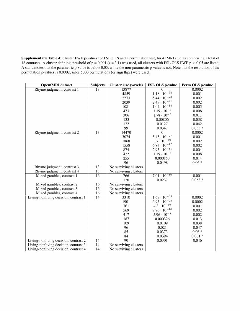
Supplementary Table 4: Cluster FWE p-values for FSL OLS and a permutation test, for 4 fMRI studies comprising a total of18 contrasts. A cluster defining threshold of p = 0.001 (z = 3.1) was used, all clusters with FSL OLS FWE p < 0.05 are listed.A star denotes that the parametric p-value is below 0.05, while the non-parametric p-value is not. Note that the resolution of thepermutation p-values is 0.0002, since 5000 permutations (or sign flips) were used.

OpenfMRI dataset Subjects Cluster size (voxels) FSL OLS p-value Perm OLS p-valueRhyme judgment, contrast 1 13 13877 0 0.0002

4859 1.18 · 10−38 0.0012273 5.44 · 10−23 0.0022039 2.49 · 10−21 0.0021081 1.04 · 10−13 0.005473 1.19 · 10−7 0.008306 1.78 · 10−5 0.011133 0.00806 0.038122 0.0127 0.04299 0.0347 0.055 *

Rhyme judgment, contrast 2 13 14470 0 0.00023074 5.43 · 10−27 0.0011868 3.7 · 10−19 0.0021558 6.83 · 10−17 0.002874 2.95 · 10−11 0.004422 1.19 · 10−6 0.008255 0.000153 0.01496 0.0498 0.06 *

Rhyme judgment, contrast 3 13 No surviving clustersRhyme judgment, contrast 4 13 No surviving clustersMixed gambles, contrast 1 16 766 7.01 · 10−10 0.001

120 0.0237 0.053 *Mixed gambles, contrast 2 16 No surviving clustersMixed gambles, contrast 3 16 No surviving clustersMixed gambles, contrast 4 16 No surviving clusters

Living-nonliving decision, contrast 1 14 3310 1.69 · 10−33 0.00021901 6.95 · 10−23 0.0002761 4.8 · 10−12 0.001569 8.96 · 10−10 0.002417 5.96 · 10−8 0.002187 0.000326 0.013109 0.0109 0.03896 0.021 0.04785 0.0373 0.06 *84 0.0394 0.061 *

Living-nonliving decision, contrast 2 14 90 0.0301 0.046Living-nonliving decision, contrast 3 14 No surviving clustersLiving-nonliving decision, contrast 4 14 No surviving clusters

Supplementary Table 5: Cluster FWE p-values for FSL OLS and a permutation test, for 4 fMRI studies comprising a total of18 contrasts. A cluster defining threshold of p = 0.001 (z = 3.1) was used, all clusters with FSL OLS FWE p < 0.05 are listed.A star denotes that the parametric p-value is below 0.05, while the non-parametric p-value is not. Note that the resolution of thepermutation p-values is 0.0002, since 5000 permutations (or sign flips) were used.

OpenfMRI dataset Subjects Cluster size (voxels) FSL OLS p-value Perm OLS p-valueWord and object processing, contrast 1 49 4644 1.4 · 10−45 0.0002

4017 2.35 · 10−41 0.00022615 7.21 · 10−31 0.0002828 6.38 · 10−14 0.001765 3.64 · 10−13 0.001543 2.57 · 10−10 0.003306 8.34 · 10−7 0.006292 1.49 · 10−6 0.006176 0.000187 0.017

Word and object processing, contrast 2 49 5000 1.4 · 10−45 0.00023902 1.61 · 10−38 0.00021540 2.22 · 10−20 0.00021199 3.92 · 10−17 0.00021035 1.84 · 10−15 0.0002989 5.6 · 10−15 0.001759 1.96 · 10−12 0.001699 9.92 · 10−12 0.001497 3.42 · 10−9 0.003413 5.96 · 10−8 0.004133 0.00222 0.02995 0.0149 0.053 *

Word and object processing, contrast 3 49 27735 0 0.00021312 2.62 · 10−19 0.0011264 8.15 · 10−19 0.001789 1.57 · 10−13 0.002525 3.99 · 10−10 0.004415 1.53 · 10−8 0.005209 4.05 · 10−5 0.013143 0.000845 0.024

Word and object processing, contrast 4 49 24890 0 0.00023525 2.79 · 10−36 0.00021678 7.98 · 10−22 0.00021492 4.01 · 10−20 0.001996 3.42 · 10−15 0.002845 1.55 · 10−13 0.003346 4.17 · 10−7 0.008112 0.00582 0.042107 0.00751 0.044106 0.00791 0.04475 0.0425 0.074 *

Word and object processing, contrast 5 49 373 2.03 · 10−8 0.005282 7.75 · 10−7 0.006109 0.00302 0.03398 0.00574 0.0492 0.00821 0.04478 0.0195 0.06 *

Word and object processing, contrast 6 49 11134 0 0.00023466 1.21 · 10−37 0.0011630 1.87 · 10−22 0.001609 2.86 · 10−11 0.003475 1.98 · 10−9 0.004270 3.16 · 10−6 0.009132 0.00145 0.025111 0.00433 0.03592 0.0123 0.04889 0.0146 0.051 *76 0.0313 0.067 *75 0.0332 0.069 *

1. REFERENCES

[1] Biswal, B. et al., “Toward discovery science of human brain function,” PNAS, vol. 107, pp. 4734–4739, 2010.

[2] J. Ashburner and K. Friston, “Voxel-based morphometry - the methods,” NeuroImage, vol. 11, pp. 805–821, 2000.

[3] C. Scarpazza, S. Tognin, S. Frisciata, G. Sartori, and A. Mechelli, “False positive rates in voxel-based morphometry

studies of the human brain: Should we be worried?,” Neuroscience & Biobehavioral Reviews, vol. 52, pp. 49–55, 2015.

[4] A. Eklund, P. Dufort, M. Villani, and S. LaConte, “BROCCOLI: Software for fast fMRI analysis on many-core CPUs and

GPUs,” Frontiers in Neuroinformatics, vol. 8:24, 2014.

[5] A. Winkler, G. Ridgway, M. Webster, S. Smith, and T. Nichols, “Permutation inference for the general linear model,”

NeuroImage, vol. 92, pp. 381–397, 2014.

[6] Worsley, K. J. et al., “A unified statistical approach for determining significant signals in images of cerebral activation,”

Human Brain Mapping, vol. 4, pp. 58 – 73, 1996.

[7] K. J. Friston, K. J. Worsley, R. S. J. Frackowiak, J. C. Mazziotta, and A. C. Evans, “Assessing the significance of focal

activations using their spatial extent,” Human Brain Mapping, vol. 1, pp. 210–220, 1994.

[8] Forman, S. D. et al., “Improved assessment of significant activation in functional magnetic resonance imaging (fMRI):

Use of a cluster-size threshold,” Magnetic resonance in medicine, vol. 33, pp. 636–647, 1995.

[9] M. Silver, G. Montana, and T. Nichols, “False positives in neuroimaging genetics using voxel-based morphometry data,”

NeuroImage, vol. 54, pp. 992–1000, 2011.

[10] C. Woo, A. Krishnan, and T. Wager, “Cluster-extent based thresholding in fMRI analyses: Pitfalls and recommendations,”

NeuroImage, vol. 91, pp. 412 – 419, 2014.

[11] A. Eklund, T. Nichols, M. Andersson, and H. Knutsson, “Empirically investigating the statistical validity of SPM, FSL

and AFNI for single subject fMRI analysis,” in IEEE International symposium on biomedical imaging (ISBI), 2015, pp.

1376–1380.

[12] Poldrack, R. et al., “Toward open sharing of task-based fMRI data: the OpenfMRI project,” Frontiers in Neuroinformatics,

vol. 7, no. 12, 2013.

[13] Kriegeskorte, N. et al., “Artifactual time-course correlations in echo-planar fMRI with implications for studies of brain

function,” International Journal of Imaging Systems and Technology, vol. 18, pp. 345–349, 2008.

cluster failure: why fmri inferences for spatial extent...

Documents