clustering algorithms for wireless sensor networks and security

Clustering algorithms for Wireless Sensor Networks

and Security threats

Master’s Thesis under Erasmus programme

CARLOS ALEIXANDRE TUDO

Department of Computer Science and Engineering

Division of Distributed Computing and Systems group

CHALMERS UNIVERSITY OF TECHNOLOGY

Goteborg, Sweden 2010

Master’s Thesis 2009:10

The Author grants to Chalmers University of Technology and University of Gothenburg

the non-exclusive right to publish the Work electronically and in a non-commercial

purpose make it accessible on the Internet.

The Author warrants that he/she is the author to the Work, and warrants that the Work

does not contain text, pictures or other material that violates copyright law.

The Author shall, when transferring the rights of the Work to a third party (for example a

publisher or a company), acknowledge the third party about this agreement. If the Author

has signed a copyright agreement with a third party regarding the Work, the Author

warrants hereby that he/she has obtained any necessary permission from this third party to

let Chalmers University of Technology and University of Gothenburg store the Work

electronically and make it accessible on the Internet.

Clustering algorithms for Wireless Sensor Network and security threats

CARLOS ALEIXANDRE TUDÓ

© CARLOS ALEIXANADRE TUDÓ, June 2010.

Examiner: Andreas Larsson

Chalmers University of Technology

University of Gothenburg


SE-412 96 Göteborg

Sweden

Telephone + 46 (0)31-772 1000


Göteborg, Sweden June 2010

MASTER’S THESIS 2009:10

Clustering algorithms for Wireless SensorNetworks and Security threats

CARLOS ALEIXANDRE TUDÓ

Department of Computing Science and EngineeringDistributed Computing and Systems Research Group

CHALMERS UNIVERSITY OF TECHNOLOGY

Göteborg, Sweden 2010

ii

Clustering algorithms for Wireless Sensor Networks and Security threats

c© CARLOS ALEIXANDRE TUDÓ, 2010

Master’s Thesis 2009:10

Department of Computing Science and EngineeringDistributed Computing and Systems Research GroupChalmers University of TechnologySE-41296 GöteborgSweden

Tel. +46-(0)31 772 1000

Department of Computing Science and EngineeringGöteborg, Sweden 2010

Clustering algorithms for Wireless Sensor Networks and Security threats

CARLOS ALEIXANDRE TUDÓDepartment of Computing Science and EngineeringDistributed Computing and Systems Research GroupChalmers University of Technology

Abstract

Since few years ago the interest of wireless sensor networks (WSNs) have been increas-ing. Furthermore a small battery sensors had appeared recently because of the minia-turization development. These new devices have a radio inside and a microprocessor,thus they can manage a big quantity of data. This new scenario has multiples advan-tages such as they can operate in hard conditions when the human can’t do or can be setup in a broad kind of systems to monitore and analyze the data. Sensors are randomlydeployed over the terrain and they have to self-organize in a small groups to achievea good power saving, scalability and routing. Thereby we need a new clustering sen-sor’s algorithms to organize these nodes in groups. In this thesis, we implement andtest some clustering algorithms to obtain the latter features. We also study which arethe security threats of our algorithm in order to see how vulnerable they are againstmalicious nodes and we will try to breakdown the system.

Keywords: WSN, Clustering algorithms, Security, TinyOS

iv

Contents

Abstract iv

Contents v

Acknowledgements ix

1 TinyOS 1

1.1 TinyOS 2.1 . . . . . . . . . . . . . . . . . . . . . . . . . . . . . . . . . . . . 11.2 NesC . . . . . . . . . . . . . . . . . . . . . . . . . . . . . . . . . . . . . . . 11.3 TOSSIM . . . . . . . . . . . . . . . . . . . . . . . . . . . . . . . . . . . . . 21.4 Our Workspace . . . . . . . . . . . . . . . . . . . . . . . . . . . . . . . . . 31.5 Example of application . . . . . . . . . . . . . . . . . . . . . . . . . . . . 4

1.5.1 Configuration file (HelloWorldAppC.nc) . . . . . . . . . . . . . . 41.5.2 Module File (HelloWorldC.nc) . . . . . . . . . . . . . . . . . . . . 6

1.6 Configuring TOSSIM . . . . . . . . . . . . . . . . . . . . . . . . . . . . . . 81.7 Security . . . . . . . . . . . . . . . . . . . . . . . . . . . . . . . . . . . . . . 8

2 LEACH algorithm 11

2.1 Description . . . . . . . . . . . . . . . . . . . . . . . . . . . . . . . . . . . . 112.2 Protocol Specification . . . . . . . . . . . . . . . . . . . . . . . . . . . . . . 12

2.2.1 Phase 1: Setup Phase . . . . . . . . . . . . . . . . . . . . . . . . . . 122.2.2 Phase 2: Steady-State Phase . . . . . . . . . . . . . . . . . . . . . . 13

2.3 Example . . . . . . . . . . . . . . . . . . . . . . . . . . . . . . . . . . . . . 13

3 Distributed cluster (Clique) algorithm 15

3.1 Description . . . . . . . . . . . . . . . . . . . . . . . . . . . . . . . . . . . . 153.2 Protocol Specification . . . . . . . . . . . . . . . . . . . . . . . . . . . . . . 153.3 Implementation . . . . . . . . . . . . . . . . . . . . . . . . . . . . . . . . . 16

3.3.1 Step 1: Local Maximum Clique . . . . . . . . . . . . . . . . . . . . 163.3.2 Step 2: Ordering and Updating Maximum Clique . . . . . . . . . 173.3.3 Step 3: Obtaining Final Clique . . . . . . . . . . . . . . . . . . . . 183.3.4 Step 4: Checking Clique Agreement . . . . . . . . . . . . . . . . . 19

4 Distributed bounded-distance multi-clusterhead algorithm 21

v

Contents

4.1 Description . . . . . . . . . . . . . . . . . . . . . . . . . . . . . . . . . . . . 214.2 Protocol Specification . . . . . . . . . . . . . . . . . . . . . . . . . . . . . . 21

4.2.1 Phase one . . . . . . . . . . . . . . . . . . . . . . . . . . . . . . . . 224.2.2 Phase two . . . . . . . . . . . . . . . . . . . . . . . . . . . . . . . . 22

4.3 Example . . . . . . . . . . . . . . . . . . . . . . . . . . . . . . . . . . . . . 24

5 New Distributed multi-clusterhead algorithm 27

5.1 Description . . . . . . . . . . . . . . . . . . . . . . . . . . . . . . . . . . . . 275.2 Protocol Specification . . . . . . . . . . . . . . . . . . . . . . . . . . . . . . 285.3 Example . . . . . . . . . . . . . . . . . . . . . . . . . . . . . . . . . . . . . 29

6 Design problems 33

6.1 How to know who are my neighbours? . . . . . . . . . . . . . . . . . . . 336.1.1 The realistic solution . . . . . . . . . . . . . . . . . . . . . . . . . . 34

6.2 Packet collisions . . . . . . . . . . . . . . . . . . . . . . . . . . . . . . . . . 356.2.1 The broadcast ACK problem . . . . . . . . . . . . . . . . . . . . . 36

6.3 Messages and Matrix type . . . . . . . . . . . . . . . . . . . . . . . . . . . 376.3.1 Boolean Matrix . . . . . . . . . . . . . . . . . . . . . . . . . . . . . 386.3.2 Integer Matrix . . . . . . . . . . . . . . . . . . . . . . . . . . . . . . 396.3.3 The solution adopted . . . . . . . . . . . . . . . . . . . . . . . . . . 40

6.4 Synchronization . . . . . . . . . . . . . . . . . . . . . . . . . . . . . . . . . 416.5 Fragmentation . . . . . . . . . . . . . . . . . . . . . . . . . . . . . . . . . . 426.6 Data compression . . . . . . . . . . . . . . . . . . . . . . . . . . . . . . . . 436.7 Tree implementation . . . . . . . . . . . . . . . . . . . . . . . . . . . . . . 43

7 Security Analisys 47

7.1 Attacks in WSN . . . . . . . . . . . . . . . . . . . . . . . . . . . . . . . . . 477.2 Security threats in TinyOS . . . . . . . . . . . . . . . . . . . . . . . . . . . 497.3 LEACH Algorithm . . . . . . . . . . . . . . . . . . . . . . . . . . . . . . . 50

7.3.1 HELLO flood attack . . . . . . . . . . . . . . . . . . . . . . . . . . 507.3.2 Sybil attack . . . . . . . . . . . . . . . . . . . . . . . . . . . . . . . 507.3.3 Other attacks . . . . . . . . . . . . . . . . . . . . . . . . . . . . . . 51

7.4 Distributed cluster (Clique) Algorithm . . . . . . . . . . . . . . . . . . . . 517.4.1 Silence attack . . . . . . . . . . . . . . . . . . . . . . . . . . . . . . 517.4.2 HELLO, Sybil and Wormhole attacks . . . . . . . . . . . . . . . . 52

7.5 Distributed bounded-distance multi-clusterhead algorithm . . . . . . . 527.5.1 Selective forwarding . . . . . . . . . . . . . . . . . . . . . . . . . . 527.5.2 Others attacks . . . . . . . . . . . . . . . . . . . . . . . . . . . . . . 53

7.6 New Distributed multi-clusterhead algorithm . . . . . . . . . . . . . . . . 537.7 Conclusions . . . . . . . . . . . . . . . . . . . . . . . . . . . . . . . . . . . 53

vi

Contents

Bibliography 55

Bibliography 55

vii

Contents

viii

Acknowledgements

Thanks to my family and Iris who always supported me throughout my career.I would like also to say my thanks to my supervisor Philippas Tsigas and my advisor

Andreas Larsson who helps me with practical processes.

ix

Contents

x

1 TinyOS

TinyOS is a free and open source component-based operating system and platform tar-geting wireless sensor networks (WSNs). It is an embedded operating system writtenin the nesC programming language as a set of cooperating tasks and processes. Thepurpose is to incorporated into small devices.

1.1 TinyOS 2.1

We will use TinyOS as the operative system for our devices. The decision to choose it isbecause of is very power efficient . Power efficient is necessary for motes due to sensorshave small-size battery, this means that they are energy-constrained and their batteriescan’t be recharged. Thus, energy is the most valuable resource and using TinyOS that ispower-efficient we can achieve our motes more time alive. TinyOS reduces the energyconsumption thanks to new internal architecture. For example in a tradition OS micro-kernel, we have large memory requirement, complex I/O subroutines, a lot of contextsswitches... All of these operations requires among quantity of energy. To reduce thisconsumption TinyOS proposes a new easy, thin and low-consumption architecture. Itchanges all this heavy process to other more simples like: only one process (no processmanagement), linear physical address space (no virtual memory), no software signals(only function call), no dynamic memory (to reduce the stack), direct hardware inter-rupts (no kernel interrupts), no kernel/user space differentiations, single share stack,etc. With it we can decrease the memory size and the system overload.

The operative system, has also a lot more features that makes it to be one of the mostpowerful embedded systems, but the aim of this thesis is it not to explain all of thesystem features.

1.2 NesC

NesC (network embedded systems C) is a dialect of the C programming language op-timized for the memory limitations of sensor networks. This programming language isused to build applications for the TinyOS platform. It has two features that makes usto develop applications for TinyOS very easy and powerful: is component-based andevent-driven. All nesC files has “.nc” extension.

1

1 TinyOS

Programs are built by modules (components), some of which present hardware ab-stractions layers (HAL) and other just high level applications. A component consists ofthree main things: frame, set of tasks and interfaces (command and events). Interfacesis the most important in the sense of how applications are organized and works. Com-ponents are connected each other using interfaces from the top layer to the bottom layerand it is the only way to access to the component. This kind model interfaces allowsthe system to have an efficient modularity. Moreover because of in the TinyOS internalcore there aren’t any signals, just call functions, these commands and events are veryefficients.

Interfaces provides command functions. This mean that we can call this routine andthe handler of the interface will execute the code of the command. Thus, as we can see,interfaces have to provide commands to let other components to use them. Commandsare usually requests from the upper layers and handled by the lower layers.

The second important feature is that nesC is event-driven. This means that the exe-cution of the program is determined by events (i.e: sensors input, timers, etc). Comingback to the components model that we talk before, that means events is just the eventscode of our interfaces. We must implement the code for these events and when thisevent will be signaled TinyOS will handler this event and execute the correspondingcode. On the other side as the commands, events usually are triggered by the lowerlayer and handled by upper layers.

To sum up we can see that TinyOS and nesC works together to provide an easy env-iorment to build our application for sensors networks. Furthermore we will have com-ponents that connects to other components using interfaces. For each interface we willprovide some commands (call functions) and we must implement the code for someevents (timer fired, data receive, etc). The Figure 1.1 show us the TinyOS and nesCcomponent model.

1.3 TOSSIM

TOSSIM (TinyOSSIMulator) simulates entire TinyOS applications. It is just a TinyOSlibrary and it works by replacing components with simulation implementations. Thelevel at which components are replaced is very flexible: for example, there is a sim-ulation implementation of millisecond timers that replaces HilTimerMilliC. Similarly,TOSSIM can replace a packet-level communication component for packet-level simula-tion, or replace a low-level radio chip component for a more precise simulation of thecode execution. Most of the real components contains a TOSSIM abstraction implemen-tation to simulate the component.

TOSSIM works as a discrete event simulator. When it runs, it pulls events of the eventqueue (sorted by time) and executes them. Additionally, tasks are simulation events, so

2

1.4 Our Workspace

Figure 1.1: Component model

that posting a task causes it to run a short time in the future.Sometimes it’s important and very useful to debug the code. TinyOS and TOSSIM

don’t have their own debugger. ETH of Zurich has developed a plug-in for Eclipsenamed Yeti2 that allow to program TinyOS applications on Eclipse and also includes adebugger. On the other hand TOSSIM give us the possibility to print out some valueson the standard output. Moreover we can configure and decided which messages wewant to show to the output.

Although the choice of using the eclipse plug-in is very attractive, I will use debugstatements providing by TOSSIM to show some important output of my applications(like packet information, battery information, routing information, error information,etc).

1.4 Our Workspace

It’s possible to run TinyOS under any Linux-like, Mac OS or Windows. Furthermorethere is a live-CD called XUbunTOS with the full operative system installed on it. Justlaunch it and you will have the full TinyOS running in your machine.

In our case, we’re going to install TinyOS in a Ubuntu Linux machine. We can choosebetween install the version 1.x or 2.x, but TinyOS 1.x is not supported right now and isdiscouraged. Hence, we will use 2.1.0 version of the system.

Concerning to TOSSIM there are also two versions: 2.0.1 and 2.0.0. There are signif-icances differences between both versions like how to specify the noise for the simu-lation. We will use the 2.0.1 version because it’s the newest. Thus, the simulator willhelp us to check how the applications work and later if we see that the program worksproperly we can install it in a set of remote sensors nodes.

3

1 TinyOS

Processor 4Mhz 8 bits AmtelMemory 4KB RAM, 512 flashRadio 916MHz, 40Kbps, 35m rangeLifetime Aprox: 2 weeks (full work)/1 year (low consumption)

Table 1.1: MICAz specifications

TinyOS runs in different kinds of chipset like CC2420 (used in micaz, telos family andimote2) or transceivers such as MICA family (MICAz, MICA2, MICA2dot), Telos family(Telosa and Telosb), TinyNode (serial port), eyesIFX-family... But TOSSIM only cansimulate the behavior of MICAz motes, not the rest of the motes. Thus, from now weare going to focus only in the MICAz model. To give an idea of the resource constraintsthe Table 1.1 shows the specification of the mote.

1.5 Example of application

On the following lines we are going to introduce an example of a very easy applicationto see how TinyOS and nesC work. We’re going to implement the “HelloWord” pro-gram. As I said before nesC is a component-oriented language programing so we haveto think as if we’re programing in a hardware description language.

To make any application we need two different types of files: module and config-uration. For convention modules are named ended “xC.nc” and configuration with“xAppC.nc”. In our example, we have two files called “HelloWorldC.nc” and “Hel-loWorldAppC.nc”. Configuration are used to assemble other components together,connecting interfaces used by components to interfaces provided by other. Every ap-plication is described by a configuration that wires together the components inside. Wecan image that components are like blocks that we have to connect each other throughinterfaces. On the other hand, we also have the module file, that provides the imple-mentation of one or more interface and uses interfaces from other modules. Modulesare those who actually implement the functionality and do the work. As we can seeinterfaces is the mechanism to wire components. They have commands that are calledby the module using the interface and events that are captured by the modules alsousing the interface. Thus, we have the schema showed in figure 1.2.

1.5.1 Con�guration �le (HelloWorldAppC.nc)

The configuration has two parts the configuration section and the implementation sec-tion.

4


Figure 1.2: Module and its basic interfaces

Algorithm 1.1 Template of the configuration file

1 configuration HelloWorldAppC{

2 .....

3 }

4 implementation{

5 ....

6 }

In the configuration braces we can specify uses and provides interfaces as with amodule. Because of helloWorld is an easy module application we don’t need to usethis.

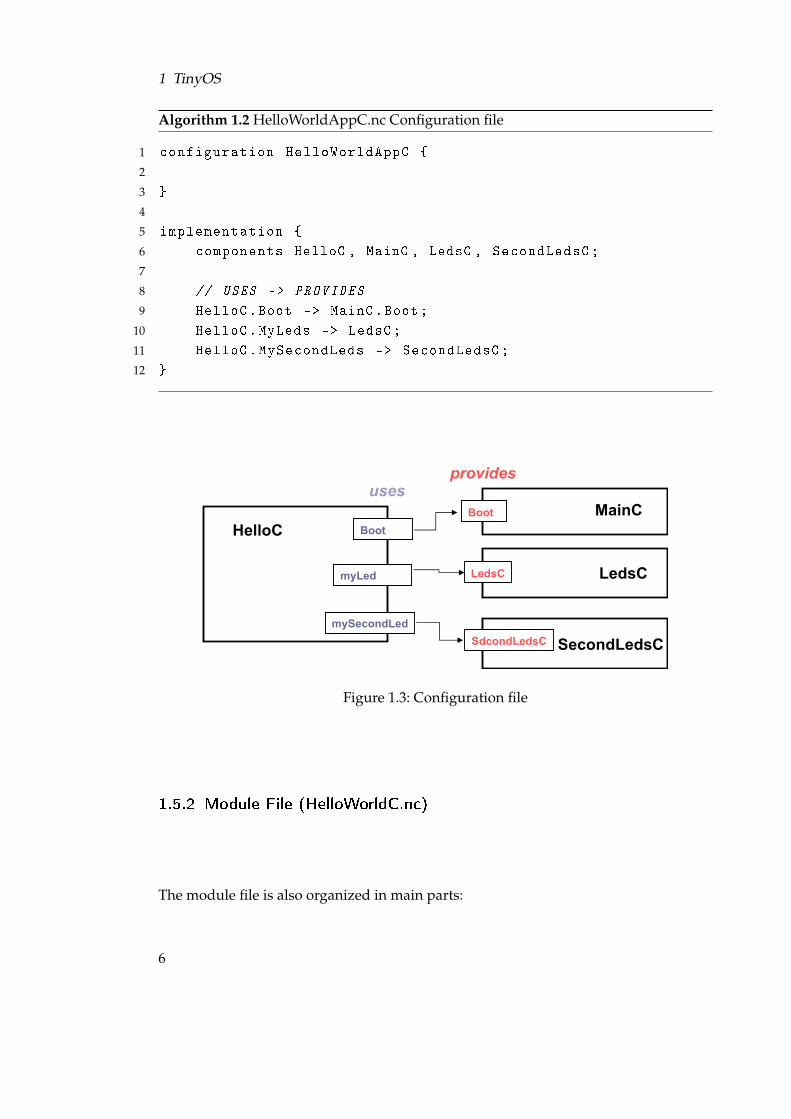
Inside the implementation part, we have to define all of the components that we’regoing to use. In our example these are: HelloP, Boot, LedsC and SecondLedsC. The lasttwo interfaces are different instances of the same interface. Thus, we can define manyinstance of the same interface as we want. The next step, is to wire interfaces used bymodules to interfaces provided by others. For example, we will connect the interfaceprovided by LedC with the interface uses by HelloC. Full code is written in algorithm1.2 and Figure 1.3 is an image representing the latter.

5

1 TinyOS

Algorithm 1.2 HelloWorldAppC.nc Configuration file

1 configuration HelloWorldAppC {

2

3 }

4

5 implementation {

6 components HelloC , MainC , LedsC , SecondLedsC;

7

8 // USES -> PROVIDES

9 HelloC.Boot -> MainC.Boot;

10 HelloC.MyLeds -> LedsC;

11 HelloC.MySecondLeds -> SecondLedsC;

12 }

Figure 1.3: Configuration file

1.5.2 Module File (HelloWorldC.nc)

The module file is also organized in main parts:

6


Algorithm 1.3 Template of module file

1 module HelloWorldC {

2 ......

3 }

4 implementation {

5 ......

6 }

In the first part, we will declare the interfaces it provides and uses. In our case weare going to use: Boot and two instances of Leds named myLed and mySecondLed. Inthe second part, we can decide what the program is going to do depend on the eventssignaled. For example when the boot event signaled we will switch on the led. We mustimplement all the events for the uses interfaces. In other words, we have to capture andhandle the events. For each interface we can see which events we must handle in theTinyOS documentation 1. Furthermore during this process we can execute commands(with the reserved word call) provided by interfaces. This is consistent with the drawon figure 1.3. Here we present the whole code of the module:

Algorithm 1.4 HelloWorldC module file code

1 module HelloWorldC {

2 uses {

3 interface Boot;

4 interface Leds as MyLeds;

5 interface Leds as MySecondLeds;

6 }

7 }

8

9 implementation {

10 event void Boot.booted () {

11 call MyLeds.led0On ();

12 call MySecondLeds.led0On ();

13 }

14 }

As we can observe this program does the following: when the system is booted led1and led2 switch on. Below is showed and intuitive draw showing this concept (redlabes indicate that we must implement this event or command):

1http://www.tinyos.net/tinyos-2.x/doc/nesdoc/micaz/

7

1 TinyOS

Figure 1.4: Components and their respective commands and events

1.6 Con�guring TOSSIM

To run TOSSIM, first we must configure the simulation and specify a network topology.The latter means that we have to decided which are the connexions between the nodes.Thus, the behavior of the link depends on two elements: the radio and the enviorment(channel) where they are placed. The radio model is based on the CC2420 and moredetails about it is found in this page2. In addition TOSSIM simulates noise too but itsaim is to provide high fidelity simulations rather than replicate the real enviorment.

We can specify the network topology either in terms of gain or in term of linkednodes. We will choose the first option and the way to said that node ’src’ is connectedwith ’dest’ is “gain src dest g”. This statement defines the propagation gain ’g’ when’src’ transmits to ’dest’. If we want to know more about this model just take a look ofthe web page at footnote 2.

To program this node connection statements, TOSSIM supports programing inter-faces written in python and C++.

1.7 Security

Security is always an issue to take into account from the mainframes to small devices.In sensor network because of communication is performed via wireless (radio), anyuser can listen the information and also inject packet.

TinyOS 1.x has a module named TinySec that implements an abstraction layer ofsome cryptographics functions to make the communication more secure. With this se-

2http://docs.tinyos.net/index.php/TOSSIM

8

1.7 Security

curity component we can run TOSSIM and check that the communication is ciphered.For TinyOS 2.x (that is actually the system that we are using) there is no secure layerimplemented to simulate with TOSSIM. Due to TinyOS 1.x is currently not supportedand discourage we will not use any cryptographics function to cipher our packages.Although if we don’t want first to simulate the behavior of the network and just wantto install the application in the nodes, motes with CC2420 transceiver has some in-linesecurity features. This tutorial 3 explain how to enable some security options in ourapplications.

Concerning to my algorithms we are going to suppose that all nodes never have amalicious behavior neither in the network nor when they are running the formationprotocol. In Section 7 we will study which are the security threats of the algorithmsimplemented.

3http://docs.tinyos.net/index.php/CC2420_Security_Tutorial

9

1 TinyOS

10

2 LEACH algorithm

Cluster algorithms can be split into two main categories: leader first approach andcluster first approach. In the leader first solution cluster head are elected based oncertain metrics, and they agree on how to assign other nodes to different clusters. Incluster first approach all the sensor nodes first form clusters, and each cluster then electsits cluster head [20]. LEACH algorithm is inside leader first cluster head group.

2.1 Description

LEACH (low-energy adaptative clustering hierarchy) is a clustering-based routing pro-tocol that uses randomized rotation of cluster heads to evenly distribute the energyload among the sensors in network [21]. This algorithm is a self-organized, adaptativeclustering protocol that the nodes organizes themselves into a local clusters, with onenode as a cluster-head. A precondition of the algorithm if that each sensor can reachthe sink, so it can be elected with the guarantee that it is going to rout the data towardthe sink.

Once the cluster is build, each CH makes a schedule that broadcast to all of its chil-dren. After this each children will transmit in its corresponding slot whitin the sched-ule. The CH have wait until all its nodes had sent their data and then the cluster willtransmit all the data aggregation to the sink. We have to remark the fact that the CH isnot always the same node, this role is rotated periodically among all nodes.

With the above model we can save up energy, because is cheaper to send data to myCH instead of transmitting packets always to the base station (it will be farther). For thecluster-head also is less energy to transmit all the data aggregation to the base stationthan sending packet per packet (because we have to send less packets and the informa-tion can be compressed). Furthermore the CH is always changing thereby allowing tobalance the load between the nodes.

In addition during the process, a TDMA schedule for the child nodes is created andeach sensor will only transmit in its corresponding slot, so in the rest of the scheduleslots they can be sleeping and save energy. If the nodes are completely synchronized, itis possible to turn off the radio until the next time of transmitting in the TDMA schedulestarts. If can not do this accurate synchronization we can use protocols like LPL (LowPower Listening) in order to keep most of the time the node sleeping and do periodicchecks to know if the radio has to switch on again. Finally another good feature of

11

2 LEACH algorithm

Figure 2.1: One round LEACH algorithm phases

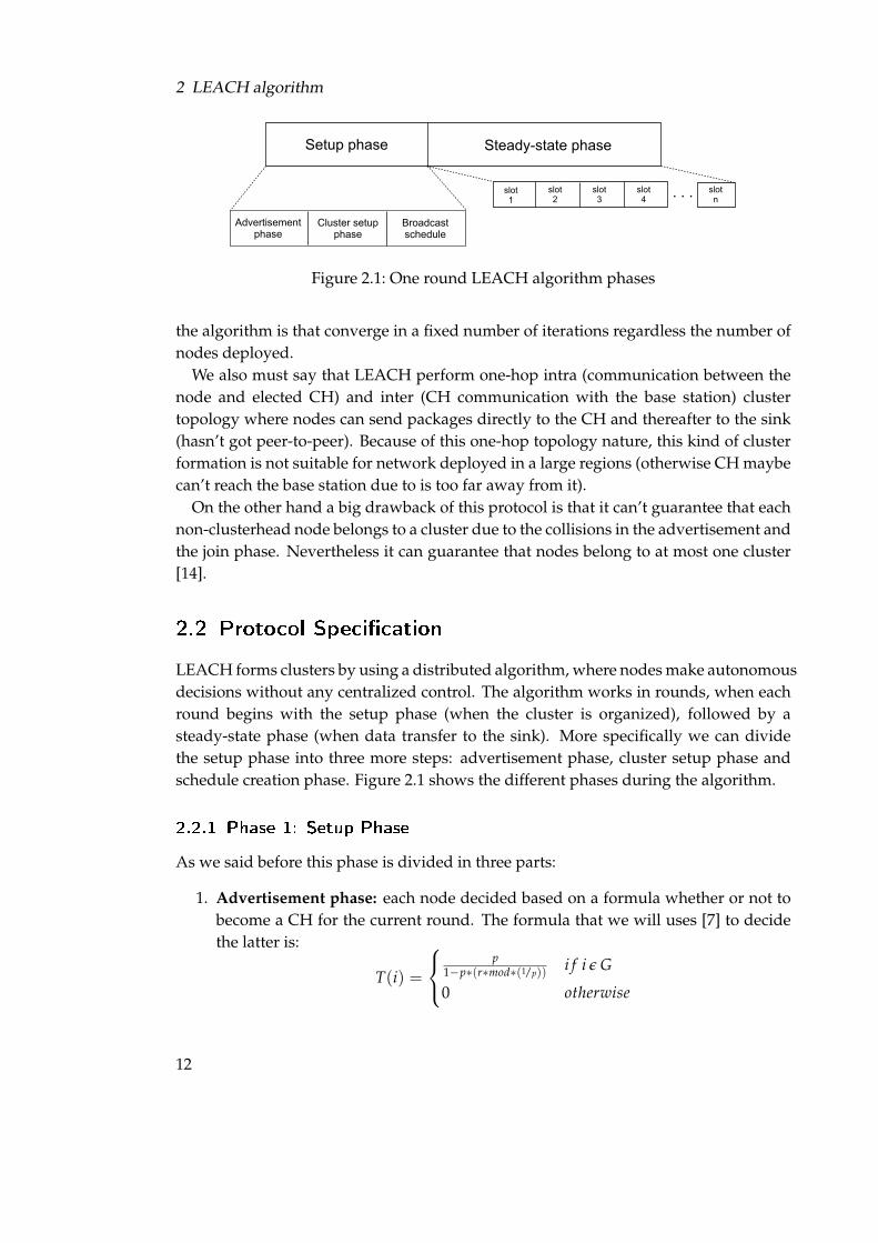
the algorithm is that converge in a fixed number of iterations regardless the number ofnodes deployed.

We also must say that LEACH perform one-hop intra (communication between thenode and elected CH) and inter (CH communication with the base station) clustertopology where nodes can send packages directly to the CH and thereafter to the sink(hasn’t got peer-to-peer). Because of this one-hop topology nature, this kind of clusterformation is not suitable for network deployed in a large regions (otherwise CH maybecan’t reach the base station due to is too far away from it).

On the other hand a big drawback of this protocol is that it can’t guarantee that eachnon-clusterhead node belongs to a cluster due to the collisions in the advertisement andthe join phase. Nevertheless it can guarantee that nodes belong to at most one cluster[14].

2.2 Protocol Speci�cation

LEACH forms clusters by using a distributed algorithm, where nodes make autonomousdecisions without any centralized control. The algorithm works in rounds, when eachround begins with the setup phase (when the cluster is organized), followed by asteady-state phase (when data transfer to the sink). More specifically we can dividethe setup phase into three more steps: advertisement phase, cluster setup phase andschedule creation phase. Figure 2.1 shows the different phases during the algorithm.

2.2.1 Phase 1: Setup Phase

As we said before this phase is divided in three parts:

1. Advertisement phase: each node decided based on a formula whether or not tobecome a CH for the current round. The formula that we will uses [7] to decidethe latter is:

T(i) =

p1−p∗(r∗mod∗(1/p))

i f i ǫ G

0 otherwise

12

2.3 Example

Where variable p allow us to decide the desired percentage of CH node in thesensor population, r is the current round number and G is the set of nodes thathave not been CHs in the last 1/p rounds. Now each node has to choose a randomnumber “T” between 0 and 1. If the random number is less than the calculatethreshold, this node will be a good candidate. After this, each node that is electedas a CH will send a broadscast message advertising all nodes. In the next stepseach non-cluster-head node decides the cluster to which it will belong for thisround depending on the signal strength or the distance.

2. Setup phase: each node has decided to which cluster belongs. The node willsend a message to the CH informing that it will be a member of that cluster. Thedecision is made based on the distance between the CH and the respective node.We will choose the nearest CH.

3. Schedule creation: CH receives all messages from nodes that would like to bein its cluster. Once the CH know the number of children, it can create a TDMAschedule, when only one node will transmit in each slot. Then the schedule isbroadcasted to the nodes members of the cluster.

2.2.2 Phase 2: Steady-State Phase

Phase 2 is the last stage, here each node will send its data to the CH during its allocatetime in TDMA schedule. When all the data has been received (data aggregation), theCH will compress the information and it will transmit this to the base station.

When the sink received all the data aggregation from the CH, it can deliver a messageto all nodes to advice that new round begins. This allow us to keep all nodes synchro-nized at the beginning of the next round, because a new round doesn’t start until thesink has received all the data from all CH. Thereafter the algorithm start again fromphase 1, choosing different CH from the previous rounds.

2.3 Example

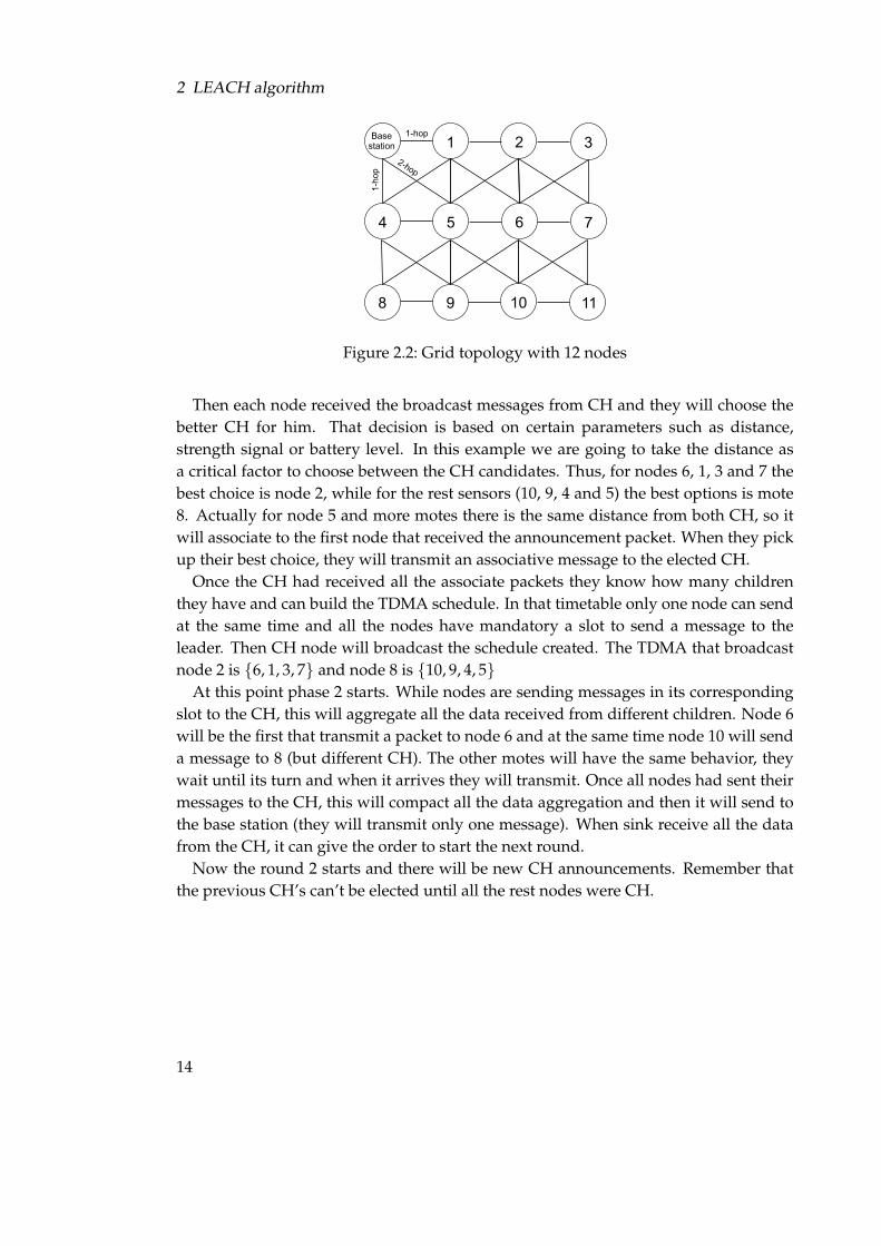
We are going to take as a reference for the example the grid topology with 12 nodes(Figure 2.2). When a new round starts, all nodes begin with the phase 1. Sensors cal-culate the T(i) value (that is T(i) = 0.2) and each node will generate a random number.In this round the only nodes that have had a number less than 0.2 are node 8 (0.1) andnode 2 (0.1). Thus, those node will became a CH and they will send an announcementmessage telling all nodes that they are CH. Moreover base station will be listening theannouncements and it will store how many CH are in the network to use it in furtheractions.

13

2 LEACH algorithm

Figure 2.2: Grid topology with 12 nodes

Then each node received the broadcast messages from CH and they will choose thebetter CH for him. That decision is based on certain parameters such as distance,strength signal or battery level. In this example we are going to take the distance asa critical factor to choose between the CH candidates. Thus, for nodes 6, 1, 3 and 7 thebest choice is node 2, while for the rest sensors (10, 9, 4 and 5) the best options is mote8. Actually for node 5 and more motes there is the same distance from both CH, so itwill associate to the first node that received the announcement packet. When they pickup their best choice, they will transmit an associative message to the elected CH.

Once the CH had received all the associate packets they know how many childrenthey have and can build the TDMA schedule. In that timetable only one node can sendat the same time and all the nodes have mandatory a slot to send a message to theleader. Then CH node will broadcast the schedule created. The TDMA that broadcastnode 2 is {6, 1, 3, 7} and node 8 is {10, 9, 4, 5}

At this point phase 2 starts. While nodes are sending messages in its correspondingslot to the CH, this will aggregate all the data received from different children. Node 6will be the first that transmit a packet to node 6 and at the same time node 10 will senda message to 8 (but different CH). The other motes will have the same behavior, theywait until its turn and when it arrives they will transmit. Once all nodes had sent theirmessages to the CH, this will compact all the data aggregation and then it will send tothe base station (they will transmit only one message). When sink receive all the datafrom the CH, it can give the order to start the next round.

Now the round 2 starts and there will be new CH announcements. Remember thatthe previous CH’s can’t be elected until all the rest nodes were CH.

14

3 Distributed cluster (Clique) algorithm

As we said in the chapter before, there are two groups of clustering algorithms: leaderfirst and cluster first. Clique algorithm belongs to cluster first set. That means thatsensors first will form clusters, and then will choose their cluster head. All nodes in thesame cluster must agree with the elected cluster head. In other words all nodes have tobe a consistent with the view of its cluster (clique) and its cluster head (CH).

3.1 Description

Clique is a cluster formation protocol that exchanging information with 1-hop neigh-bors sensors nodes are divided into mutually disjoints cluster (cliques). The protocolaims to divide the sensor network into multiples small groups and guarantees that allthe nodes in each clique agree on the same clique membership. The protocol has thefollowing properties:

• It is full distributed. Each node computes its clique only using information fromits 1-hop neighbors.

• It is guarantee to terminate.

• After protocol terminates, all nodes are divided into mutually disjoint clique.They have consistent view on their clique membership.

The original algorithm [20] assumes that each node knows its 1-hop neighbors and theyhave and unique ID.


The protocol is divided in four steps:

1. Each node exchanges its neighbor list with its neighbors, and computes its localmaximum clique.

2. Each node exchanges its local maximum clique with its neighbors, and update itsmaximum clique according to its neighbor nodes local maximum clique.

15


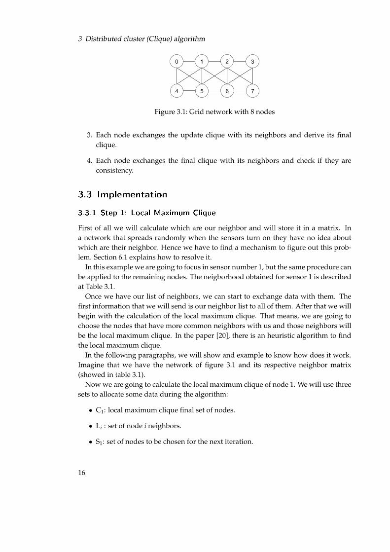
Figure 3.1: Grid network with 8 nodes

3. Each node exchanges the update clique with its neighbors and derive its finalclique.

4. Each node exchanges the final clique with its neighbors and check if they areconsistency.

3.3 Implementation

3.3.1 Step 1: Local Maximum Clique

First of all we will calculate which are our neighbor and will store it in a matrix. Ina network that spreads randomly when the sensors turn on they have no idea aboutwhich are their neighbor. Hence we have to find a mechanism to figure out this prob-lem. Section 6.1 explains how to resolve it.

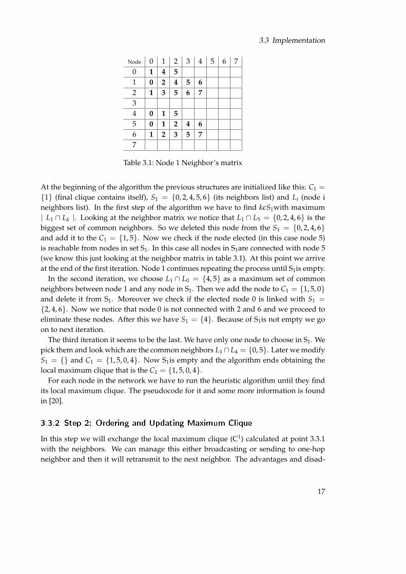
In this example we are going to focus in sensor number 1, but the same procedure canbe applied to the remaining nodes. The neigborhood obtained for sensor 1 is describedat Table 3.1.

Once we have our list of neighbors, we can start to exchange data with them. Thefirst information that we will send is our neighbor list to all of them. After that we willbegin with the calculation of the local maximum clique. That means, we are going tochoose the nodes that have more common neighbors with us and those neighbors willbe the local maximum clique. In the paper [20], there is an heuristic algorithm to findthe local maximum clique.

In the following paragraphs, we will show and example to know how does it work.Imagine that we have the network of figure 3.1 and its respective neighbor matrix(showed in table 3.1).

Now we are going to calculate the local maximum clique of node 1. We will use threesets to allocate some data during the algorithm:

• C1: local maximum clique final set of nodes.

• Li : set of node i neighbors.

• S1: set of nodes to be chosen for the next iteration.

16

3.3 Implementation

Node 0 1 2 3 4 5 6 70 1 4 5

1 0 2 4 5 6

2 1 3 5 6 7

34 0 1 5

5 0 1 2 4 6

6 1 2 3 5 7

7

Table 3.1: Node 1 Neighbor’s matrix

At the beginning of the algorithm the previous structures are initialized like this: C1 =

{1} (final clique contains itself), S1 = {0, 2, 4, 5, 6} (its neighbors list) and Li (node ineighbors list). In the first step of the algorithm we have to find kǫS1with maximum| L1 ∩ Lk |. Looking at the neighbor matrix we notice that L1 ∩ L5 = {0, 2, 4, 6} is thebiggest set of common neighbors. So we deleted this node from the S1 = {0, 2, 4, 6}and add it to the C1 = {1, 5}. Now we check if the node elected (in this case node 5)is reachable from nodes in set S1. In this case all nodes in S1are connected with node 5(we know this just looking at the neighbor matrix in table 3.1). At this point we arriveat the end of the first iteration. Node 1 continues repeating the process until S1is empty.

In the second iteration, we choose L1 ∩ L0 = {4, 5} as a maximum set of commonneighbors between node 1 and any node in S1. Then we add the node to C1 = {1, 5, 0}and delete it from S1. Moreover we check if the elected node 0 is linked with S1 =

{2, 4, 6}. Now we notice that node 0 is not connected with 2 and 6 and we proceed toeliminate these nodes. After this we have S1 = {4}. Because of S1is not empty we goon to next iteration.

The third iteration it seems to be the last. We have only one node to choose in S1. Wepick them and look which are the common neighbors L1 ∩ L4 = {0, 5}. Later we modifyS1 = {} and C1 = {1, 5, 0, 4}. Now S1is empty and the algorithm ends obtaining thelocal maximum clique that is the C1 = {1, 5, 0, 4}.

For each node in the network we have to run the heuristic algorithm until they findits local maximum clique. The pseudocode for it and some more information is foundin [20].

3.3.2 Step 2: Ordering and Updating Maximum Clique

In this step we will exchange the local maximum clique (C1) calculated at point 3.3.1with the neighbors. We can manage this either broadcasting or sending to one-hopneighbor and then it will retransmit to the next neighbor. The advantages and disad-

17


Node 0 1 2 3 4 5 6 70 0 1 4 5

1 1 5 0 4

2 2 6 1 5

34 4 0 1 5

5 5 1 0 4

6 6 2 1 5

7

Table 3.2: After step 1: node 1 local maximum clique (C11)

vantages of this is discussed at section 6.1. Once we have received all the local maxi-mum clique from my neighbors we are going to order all of clique to check if there isany C1

i which is better than C1j . We can say that C1

i > C1j if:

• Both cliques C1j and C1

i mandatory have to contain node k.

• If | C1i |>| C1

j |, then C1i > C1

j .

• If | C1i |=| C1

j |, we compare the index. If i > j then C1i > C1

j .

Let us to illustrate the latter with an example. For the network in image 3.1, we have thelocal maximum clique of node 1 on table 3.2. As we have said before nodes exchangestheir local maximum clique with its neighbors.

Now we are going to order the cliques received to know which is the best clique fornode 1 (C2

1). First of all, we check if all cliques (C1j ) in the table contain node 1. If it

isn’t we can’t compare these cliques and we have to drop the clique (C1j ). In this case

all cliques (0,2,3,4,5,6) have node 1 in its list of nodes. So, we don’t delete any clique.After this, we compare the length of the cliques and order them from the largest to theshortest. Here we can notice that all of our cliques have the same length. To breakthis tie we will choose the clique of its bigger neighbor ID. The ordered list of node 1’scliques is: C6 > C5 > C4 > C2 > C0 and the C2

1 = {6, 2, 1, 5}.

3.3.3 Step 3: Obtaining Final Clique

Each node broadcast its update clique C2i to their neighbors. For every node j in C2

i ,node i check if it’s included in j’s clique C2

j . If not, node i removes j from its clique C2j .

After this step, each node i has its final clique C3i .

For our example in figure 3.1 the next table show as the result after step 2:For node 1 example the clique is C2

1 = {6, 2, 1, 5}. If we check C26 = {7, 2, 3, 6} we

can notice that sensor 1 is not in the list. Thus we remove node 6 from our final clique.

18

3.3 Implementation

Node 0 1 2 3 4 5 6 70 5 1 0 4

1 6 2 1 5

2 7 2 3 6

34 5 1 0 4

5 6 2 1 5

6 7 2 3 6

7

Table 3.3: After step 2: node 1 updating maximum clique (C21)

Figure 3.2: Final cliques for grid network with 8 nodes

The same occurs for node 2, which the clique is C22 = {7, 2, 3, 6} and again node 1 is not

included, consequently we have to drop out node 2 from our list. The next sensor is idfive and its clique is C2

5 = {5, 1, 0, 4}. I we check out the set we find out node 1 is inside,so we keep this node in the list. At the end the final clique is: C3

1 = {1, 5}.

3.3.4 Step 4: Checking Clique Agreement

After step 3, we can guarantee the clique agreement. Now each node just broadcasttheir final clique (C3

i ). Then nodes verifies the clique agreement, that is, node i verifiesfor all jǫC3

i , whether C3i = C3

j holds. In the Figure 3.2 we can see the final cliquesobtained for every sensor at the end of the protocol.

19


20

4 Distributed bounded-distance

multi-clusterhead algorithm

Bounded-distance multi-clusterhead formation algorithm (Spohn and Garcia-Luna-Aceves[19]) is a distributed clustering using (k,r)-dominating sets. Any node is said to be(k,r)-dominated if node i has at least k neighbors with distance r in D. This multi-clusterhead protocol allow the nodes to have several CH (redundancy) in order to havefault-tolerance for the applications. If we go on with the two differents approach forclustering algorithm (leader-first and cluster-first), this algorithm will be included inthe leader-first group due to at the beginning nodes try to find out which are its bestCH and then join them. In this chapter we will see which are the goals of have a cluster(or a multi-cluster) and how to perform them.

4.1 Description

In the WSN’s field, a cluster is a group of linked sensors. This kind of structures is veryuseful in WSN’s, because it can helps to achieve an increase of timelive, balance theload in the network and good scalability. Thus, clustering is the problem of buildinghierarchy among nodes (clusters) [9]. Each cluster has one node that represents it, that isthe cluster-head (CH). Thereby the network can be abstracted such just the connectionbetween cluster-heads.

To achieve these clusters usually we have first to calculate the dominating set (DS)of the network. The domination problem seeks to determine the minimum numbersof nodes D (called dominating nodes or cluster heads) such that any node i not in D isadjacent to at least one node in D [19]. This problem is NP-complete.

For the (k,r)-Dominating set problem, r defines the maximum distance from nodes totheir cluster-heads and k the minimum numbers of dominating sets per node. We cannotice that with a k greater than one we have redundancy that we can use it to buildfault-tolerant applications.


The Spohn algorithm has two main phases. The first is called election phase and hereeach node elects k nodes with small ID (also including itself) with distance r. This

21

4 Distributed bounded-distance multi-clusterhead algorithm

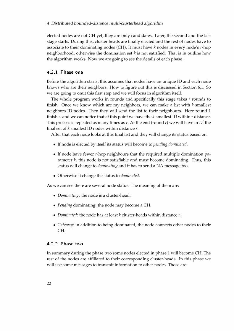
elected nodes are not CH yet, they are only candidates. Later, the second and the laststage starts. During this, cluster heads are finally elected and the rest of nodes have toassociate to their dominating nodes (CH). It must have k nodes in every node’s r-hopneighborhood, otherwise the domination set k is not satisfied. That is in outline howthe algorithm works. Now we are going to see the details of each phase.

4.2.1 Phase one

Before the algorithm starts, this assumes that nodes have an unique ID and each nodeknows who are their neighbors. How to figure out this is discussed in Section 6.1. Sowe are going to omit this first step and we will focus in algorithm itself.

The whole program works in rounds and specifically this stage takes r rounds tofinish. Once we know which are my neighbors, we can make a list with k smallestneighbors ID nodes. Then they will send the list to their neighbours. Here round 1finishes and we can notice that at this point we have the k-smallest ID within r distance.This process is repeated as many times as r. At the end (round r) we will have in D′

i thefinal set of k smallest ID nodes within distance r.

After that each node looks at this final list and they will change its status based on:

• If node is elected by itself its status will become to pending dominated.

• If node have fewer r-hop neighbours that the required multiple domination pa-rameter k, this node is not satisfiable and must become dominating. Thus, thisstatus will change to dominating and it has to send a NA message too.

• Otherwise it change the status to dominated.

As we can see there are several node status. The meaning of them are:

• Dominating: the node is a cluster-head.

• Pending dominating: the node may become a CH.

• Dominated: the node has at least k cluster-heads within distance r.

• Gateway: in addition to being dominated, the node connects other nodes to theirCH.

4.2.2 Phase two

In summary during the phase two some nodes elected in phase 1 will become CH. Therest of the nodes are affiliated to their corresponding cluster-heads. In this phase wewill use some messages to transmit information to other nodes. Those are:

22

4.2 Protocol Specification

• Local advertisement (LA): a message with the list of elected node by the node i

and their respective next-hop of that elected node.

• Neighborhood advertisement (NA): a message advertising a CH.

• Notification: a message send to notify a node that must become a CH.

• Join: a message associate to a CH.

First of all dominated nodes send only to their one-hop neighbours a LA message. Anydominated node i that receives the LA packet will do:

1. If node i is listed in the list of LA message, node i changes it status to dominating

and it will send a NA message announcement itself as a CH. This is accomplishedby broadcasting NA message using restricted blind-flooding with the TTL fieldset equal to r.

2. If node i is not listed in the list of LA message received but is listed as a next-hopof any advertised node, then node i changes its status to gateway.

3. For any advertised node a that is not among the nodes elected by node i (is not inD′

i) and the node is in the path to a, it must send a notification message to a.

Once all local advertisement messages have been received, nodes that have to send anotification message to some mote (because of the previous point 3) it is time to do it.With this process any node that receives a notification package must become CH. Afterthat, sensors that have pending NA messages to transmit (due to the point 1 above orphase one) it will send them.

NA messages are delivered using blind-flooding that means all nodes whitin r-hopdistance will receive the packet. For each NA message that we listen we will validatedthat node. This is the same as saying, for any node i and for all nǫD′

i , node n is deemedvalidated only upon the reception of the respective NA message advertising node n;otherwise the node n is not yet validated [19].

Now we will check if the agreement has reached. We will wait a period of time that isdefined as the minimum time required for reaching an agreement in phase two. Afterthis period if node i is pending dominating and it does not have enough validated en-tries in D′

i , then node i changes status to dominating, and send a NA message. Otherwiseany non-dominating node i sends a join message to k nodes from D′

i [19]. Like notifi-cation messages, join packet also assigns gateway status the node when the message isbeing routed. That is, if the receiver node is not the target, it will change its status togateway and will relay the message. How message are retransmitted is discussed insection 6.2.

23


Figure 4.1: Grid topology network with 12 nodes

4.3 Example

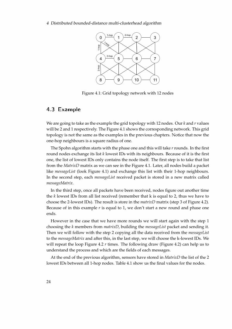
We are going to take as the example the grid topology with 12 nodes. Our k and r valueswill be 2 and 1 respectively. The Figure 4.1 shows the corresponding network. This gridtopology is not the same as the examples in the previous chapters. Notice that now theone-hop neighbours is a square radius of one.

The Spohn algorithm starts with the phase one and this will take r rounds. In the firstround nodes exchange its list k lowest IDs with its neighbours. Because of it is the firstone, the list of lowest IDs only contains the node itself. The first step is to take that listfrom the MatrixD matrix as we can see in the Figure 4.1. Later, all nodes build a packetlike messageList (look Figure 4.1) and exchange this list with their 1-hop neighbours.In the second step, each messageList received packet is stored in a new matrix calledmessageMatrix.

In the third step, once all packets have been received, nodes figure out another timethe k lowest IDs from all list received (remember that k is equal to 2, thus we have tochoose the 2-lowest IDs). The result is store in the matrixD matrix (step 3 of Figure 4.2).Because of in this example r is equal to 1, we don’t start a new round and phase oneends.

However in the case that we have more rounds we will start again with the step 1choosing the k members from matrixD, building the messageList packet and sending it.Then we will follow with the step 2 copying all the data received from the messageList

to the messageMatrix and after this, in the last step, we will choose the k-lowest IDs. Wewill repeat the loop Figure 4.2 r times. The following draw (Figure 4.2) can help us tounderstand the process and which are the fields of each messages.

At the end of the previous algorithm, sensors have stored in MatrixD the list of the 2lowest IDs between all 1-hop nodes. Table 4.1 show us the final values for the nodes.

24

4.3 Example

Figure 4.2: Spohn data structures and data flow

MatrixD={{Id,Node Adv,Dist},...} MatrixD={{Id,Node Adv,Dist},...}

Node0 {{0,0,0},{1,1,1}} Node6 {{1,1,1},{2,2,1}}Node1 {{0,0,1},{1,1,0}} Node7 {{2,2,1},{3,3,1}}Node2 {{1,1,1},{2,2,0}} Node8 {{4,4,1},{5,5,1}}Node3 {{2,2,1},{3,3,0}} Node9 {{4,4,1},{5,5,1}}Node4 {{0,0,1},{1,1,1}} Node10 {{5,5,1},{6,6,1}}Node5 {{0,0,0},{1,1,1}} Node11 {{6,6,1},{7,7,1}}

Table 4.1: MatrixD values after phase 1

Now nodes change its status as follow: node 0, 1, 2 and 3 are self-elected nodes,so their status will be pending dominating. The rest of sensors have the status set todominated. At this point phase one of Spohn algorithm finishes.

First of all in the phase 2 all dominated nodes have to send a LA message to theirone-hop neighbor. Nodes 4, 5, 6 and 7 will receive that message from nodes 8,9,10 and11, thereby nodes 4,5,6 and 7 will become a dominating node and later they will send aNA message. Sensors 0,1,2 and 3 because they are pending dominated nodes that don’tchange their status to dominating and they are still pending. Any node has to send a

25


notification message due to all advertised nodes are among the nodes elected (matrixD).All nodes that have NA message to send, it is time to do it. Nodes 4,5,6 and 7 will

transmit the NA packet to their neighbours. Each node that received the message willadd this mote to the matrixD and also will validate the node. After all messages havebeen processed the matrixD of sensors are the values on Table 4.2.

MatrixD={{Id,Node Adv,Dist},...} MatrixD={{Id,Node Adv,Dist},...}

Node0 {{4,4,1},{5,5,1}} Node6 {{-,-,-},{-,-,-}}Node1 {{4,4,1},{5,5,1}} Node7 {{-,-,-},{-,-,-}}Node2 {{5,5,1},{6,6,1}} Node8 {{4,4,1},{5,5,1}}Node3 {{6,6,1},{7,7,1}} Node9 {{4,4,1},{5,5,1}}Node4 {{-,-,-},{-,-,-}} Node10 {{5,5,1},{6,6,1}}Node5 {{-,-,-},{-,-,-}} Node11 {{6,6,1},{7,7,1}}

Table 4.2: MatrixD values after receiving the NA message

The next step is to check the agreement. Because all pending dominating have enoughvalidated entries in matrixD they will change their status to dominated. After that, allnodes send a join message to their elected nodes. We can see the final network andwhich are the dominating and dominated nodes at Figure 4.3 .

Figure 4.3: Dominated and dominating nodes after Spohn algorithm

26

5 New Distributed multi-clusterhead

algorithm

In the last algorithm there are some topologies where the Spohn-Garcia protocol choosestoo many dominating nodes (cluster heads). Our goal now is to provide a good perfor-mance for all topologies (not the optimal for all cases, but always a good solution). Theprotocol also assures that each node will have k cluster heads within r hops. Further-more this new implementation will save all the possible paths from the node to all itsneighbors in order to support fault-tolerance if a link or path break-down.

5.1 Description

Distributed bounded-distance multi-clusterhead algorithm (see Chapter 4) usually cal-culates the optimal number the cluster. However there are topologies such a chaintopologies (Figure 5.1) where the performance of this protocol is not very good. In thecase of the latter network, the number of CH chooses by Spohn-Garcia are {1,2,3,4,5,6,7,8},but in fact the best solution is to elect as a CH nodes {0,2,5,8}. To solve bad achievementswe propose a new algorithm, that has a good fulfillment in all cases, but it’s not alwaysthe optimal result.

In the new protocol a node can adopt three possible states: slave, head or escaping.Now, the idea is that each node picks up some node to be their CH. Then, could be that anode that is elected to be a CH (so its state is head) can have within its r-hop more than k

heads nodes. In that case, this node will try to escape and become a normal node (slave).Thus, a node will inform their neighbor that it’s trying to escape and if all sensors allowhim to escape (in order words, any sensor doesn’t need him as CH because there areothers to fulfill its coverage) it will convert in slave mote. The procedure is repeateduntil the network converges to a state where all nodes states don’t change anymore(any head node try to escape).

Another good feature is the fact that the algorithm can be launched in inconsistency

Figure 5.1: Chain network and CH elected by Spohn-Garcia

27

5 New Distributed multi-clusterhead algorithm

states. In Spohn-Garcia algorithm to run the network it is mandatory to know whichare our neighbors and then chooses the k-smallest. In our new implementation is notnecessary to learn this information (the protocol can be launched without have learntour neighborhood before).

A drawback is that the protocol has to send many messages that be don’t know be-forehand until the network converge (it doesn’t converge in fixed known rounds).

In addition, our algorithm supplies the full path from one node to all its neighbors.This can be used for faul-tolerant applicantions and it gives us the possibility to rout theinformation through several paths depends on some condition. However if we wantthis new feature, the number of packets sent and received will increase a lot in orderto maintain the full tree (all possible path from the main node to the others). TinyOSdoesn’t support a big payload in its messages so we have to use some compressiontechniques to reduce the size of the message as well as a more elaborated mechanismto transmit the tree between our neighborhood (see Section 6.6).


The protocol works in rounds. Each round is divided in three steps:

1. Phase one. This phase will determine our state, generate a random number toescape and calculate the set of nodes to join.

2. Phase two: send join message to all members in the join list. If node get a joinmessage it will become cluster head.

3. Phase three: if a node has modified its state, it has to send a message to theirneighborhood advertising them. The nodes will update the status of their neigh-bors.

These tree stages will looped indefinitely until the network converge to a stable state.The phase where all the hard work is done is the first one. There first of all, each

node updates it set of head nodes (they know that information because in step threeall nodes excahnge its status) and save them in a join list. In the case that we haven’tgot enough head nodes to fulfill the coverage, we can pick up another mote that is notCH but it’s in our neighborhood. Then CHs nodes which have more than k head in itslist will try to escape from being a CH and become a slave. This is done by choosing arandom number, so every of the previous nodes will have the chance to abdicate, butall them will not do at the same time. Nodes that have the opportunity to escape willchange its state to escaping.

Here phase two starts. Each node sends a join message to its elected join nodes (cal-culated at point one). When a node receives a join message if he is not trying to escape

28

5.3 Example

it will become a head. However if a node is trying to escape it will maintain its status toescaping.

In phase three all nodes will transmit its state. When a node receives node with stateequal to head, it will update its list of head nodes within its neighborhood (if it hasn’tgot it yet). Nevertheless if it receives a message from a node with the escaping statethe node will checks its coverage. If it has enough head nodes to fulfill the coverage, itwill delete the node from its head list (allowing that node to escape). However if themote hasn’t got enough head, it will not let the node to escape. That means in followingrounds it will get a join message.

After the description of the protocol a question can arise, how can a node doesn’t letanother to escape if when the status is escaping the nodes don’t ignore join messages?The solution is because there is a pseudostate called hoping that takes one round afterthe escaping state when if any node send a join message to a sensor it will become clusterhead. If during this hoping state a node doesn’t obtain any join message it will convertto slave.

5.3 Example

Let’s take the chain topology at Figure 5.1 to see how does the protocol works and tocompare with Spohn-Garcia algorithm. The parameters are k = 1 and r = 1.

At the beginning nodes don’t know anything about its neighbors, so all become heads.Now, because they have modified its state, sensors transmit a message informing theothers that they are head.

At this point phase one starts. Each node updates their list of head nodes receivedbefore. After that, every sensor realizes that it has more head that the needed to fulfillits coverage (see Table 5.1). and because they are heads node select a random numberfor attempting to escape and become a slave mote. The arbitrary numbers and moreinformation of this example are showed in Table 5.1.

Node 0 1 2 3 4 5 6 7 8 9

State head head head head head escp head head head head

Join set {1} {0,2} {1,3} {2,4} {3,5} {4,6} {5,7} {6,8} {7.,9} {8}

Random 3 10 5 2 1 0 6 11 7 12

Table 5.1: Nodes information in round 0

As we can observe, the first mote that it has a chance to escape is number 5 (inter-nally we have another timer that increases from 0 till a defined constant and give thepossibility to all heads to abdicate).

In the second phase, nodes send to their heads a join message. In the Table 5.1 we can

29


see the list of join messages that we are going to send. When a node receives a join itwill convert into a head mote, except the node which is trying to escape (which its stateis equal to escape). The Table 5.1 will show which are the states after the join messageshave been received.

In the third phase nodes deliver a packet telling to their neighbors which is theirupdate state after received a join message. At this moment when nodes 4 and 6 receivefrom node 5 the state escaping, they will check if they have enough nodes to accomplishthe k-cluster head whitin r-hop distance. In this case nodes 4 and 6 have more heads intheir list to fulfill the coverage (such as 3 and 7 respectively), so they will allow node 5to escape by deleting it from their list of head nodes (that entails that these nodes willnot send a join message any more to node 5).

At this time, a new round starts again. This is specially important for node 5 due toit is now in a pseudostate named hoping and if during this round anyone send a joinmessage to him it will convert from hoping to slave.

The first step in this new round is phase one, which all nodes updates their list ofhead nodes for later send a message to them. Furthermore if the internal timer forescaping heads has reached any node, it will have the chance to abdicate. Table 5.2summarizes all the important nodes information.

Node 0 1 2 3 4 5 6 7 8 9

State head head head head escp hop head head head head

Join {1} {0,2} {1,3} {2,4} {3} {4,6} {7} {6,8} {7,9} {8}

Rand 3 10 5 2 1 0 6 11 7 12

Table 5.2: Nodes information in round 1

In phase two, nodes will send join messages to their elected heads. In the case ofsensor 4, because its state is escaping when it receives the join message from node 3 and5 it will not become a head node. The others, when they get the packet with their Id inthe message data field, it will convert to head. In addition, as we can see, any node isgoing to send a join message to node 5. Thus, node 5 will be finally a slave node due toanyone has requested it in this round.

At the beginning of phase three all nodes exchange their state. Nodes 3 and 5 receivesfrom node 4 that their new status is escaping. As a consequence of this, they check ifthey more or equal to k head nodes in their list. Because both nodes (3 and 5) haveto elements in their list and it only necessary one head per node, they allow node 4 toescape by deleting it from its head record.

Now a new round is going to start and we can observe all the necessary informationin Table 5.3.

Again every node will update their heads nodes list, for further send a join message

30

5.3 Example

Node 0 1 2 3 4 5 6 7 8 9

State head head head escp hop slave head head head head

Join {1} {0,2} {1,3} {2} {3} {6} {7} {6,8} {7,9} {8}

Rand 3 10 5 2 1 - 6 11 7 12

Table 5.3: Node information in round 2

to them. Because the internal timer for escaping nodes is equal to the random numberof mote 3, this sensor will attempt to escape and become a slave.

In the next phase, sensors will send their corresponding join messages to their electedheads. As we can notice sensor 4 which is in the pseudostate hoping, will not receiveany message from its neighbors. Thus at the end of this round it will be a slave node.Moreover number 3 will get a join message from two but because of it is escaping itwill ignore the message and don’t become in head. The rest of motes that acquire joinmessage will be set as a head.

At the third stage nodes exchange its new states. Node 3 will get that sensor 2 is aescaping node (trying to abdicate as a head node), but if it checks its coverage it hasn’tgot enough heads to fulfill the requirements (k heads). Thereby node 4 doesn’t deletethree from its list of heads and consequently in the next mote 3 will get a join message.On the contrary, in the case of number 2 it has enough heads in its list, so it will deletenode 3 from the record. Here we find a curious situation, because mote 2 allow node 3to escape but node 3 not. The results is that if all nodes are not agree with the escapingsituation the sensor will not escape.

Round number 2 is finish and now round three begins. All the important data for thenext steps is displayed in Table 5.4.

Node 0 1 2 3 4 5 6 7 8 9

State escp head head hop slave slave head head head head

Join {1} {0,2} {1} {2} {3} {6} {7} {6,8} {7,9} {8}

Rand 3 10 5 2 - - 6 11 7 12


The important issue in this round is the fact that node 3 which is in the pseudostate ofhoping, will receive a join message from node 3. This action will lead node 3 to becomein head again, picking up a new random number to have the change to escape in futuretime. Table 5.5 will show another round of the algorithm.

When the algorithm ends we can get a result similar to Table 5.6 and the Figure 5.2,but we have to keep in mind that each time that we run the algorithm we can getdifferent results because all depends on the random number that is generated which

31


Node 0 1 2 3 4 5 6 7 8 9

State hop head head head slave slave head head head head

Join {1} {2} {1} {2} {3} {6} {7} {6,8} {7,9} {8}

Rand 3 10 5 7 - - 6 11 7 12


allow nodes to escape following a certain order.

Node 0 1 2 3 4 5 6 7 8 9

State slave head slave head slave slave head head slave head

Join {1} {-} {1,3} {-} {3} {6} {7} {6} {7,9} {-}

Rand - 10 - 7 - - - 11 - 12

Table 5.6: Final result of the algorithm

Figure 5.2: CH elected in our algorithm for the chain network

One of the advantages of this algorithm if we compare with the Spohn-Garcia is thatwe get less heads in this special topologies. For other topologies we can obtain moreheads than Spohn algorithm, but our algorithm will always achieve a good perfor-mance. On the other hand the drawback of the protocol is that it takes some undefinedrounds (as Spohn but not fixed round like LEACH) to converge as well as it has to senda lot if messages.

32

6 Design problems

During the implementation of the algorithms problems sometimes arises that are notdirectly related with itself but it is mandatory to figure out them to run the algorithmproperly. For example most of them assumes that each nodes knows its neighbour. Inour case if we want to run the algorithm in the network or in the simulator, we have tosolve these assumptions and find out which are our neighbours. Some of troubles citedbelow could be the topic of a whole thesis, however in this work we won’t go into deepand we will choose just a suitable solution.

In this chapter we discuss which are these problems found during the implementa-tion of the algorithms and how to work out them .

6.1 How to know who are my neighbours?

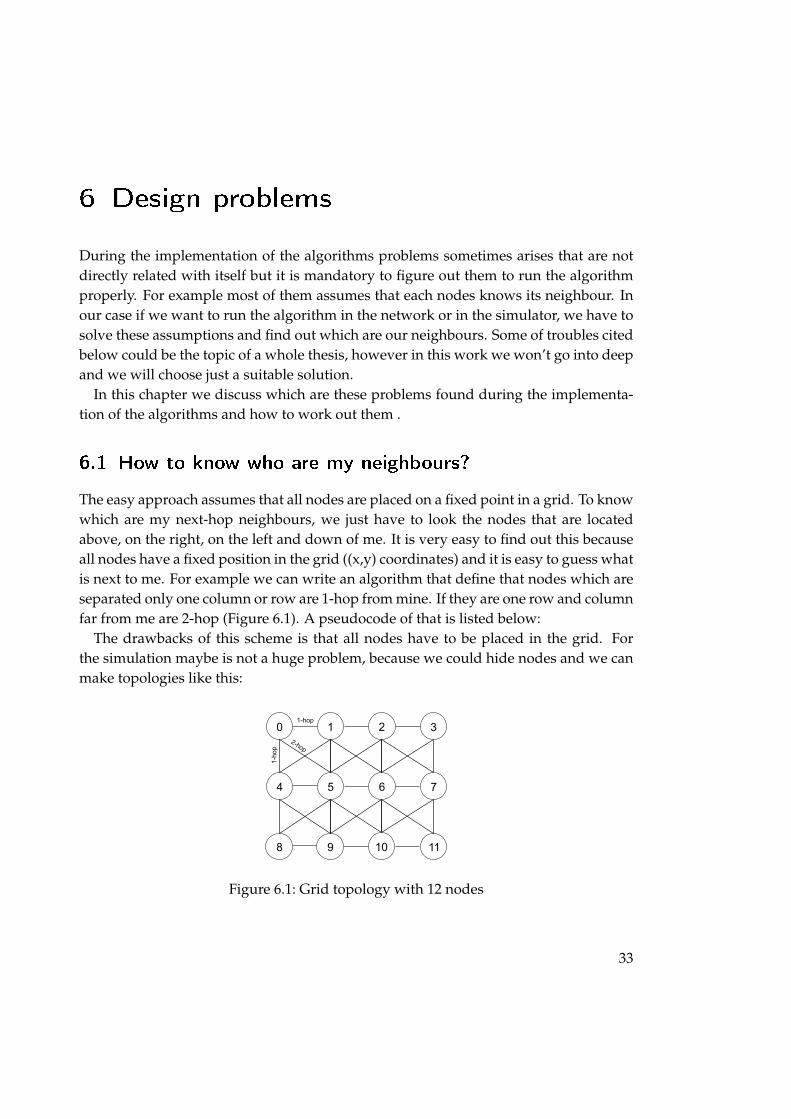
The easy approach assumes that all nodes are placed on a fixed point in a grid. To knowwhich are my next-hop neighbours, we just have to look the nodes that are locatedabove, on the right, on the left and down of me. It is very easy to find out this becauseall nodes have a fixed position in the grid ((x,y) coordinates) and it is easy to guess whatis next to me. For example we can write an algorithm that define that nodes which areseparated only one column or row are 1-hop from mine. If they are one row and columnfar from me are 2-hop (Figure 6.1). A pseudocode of that is listed below:

The drawbacks of this scheme is that all nodes have to be placed in the grid. Forthe simulation maybe is not a huge problem, because we could hide nodes and we canmake topologies like this:

Figure 6.1: Grid topology with 12 nodes

33

6 Design problems

Algorithm 6.1 Distance between nodes

1 int distanceBetweenXY(int ax,int ay,int bx,int by)

2 {

3 return (bx - ax) * (bx-ax) + (by - ay) * (by-ay);

4 }

5

6 int distanceBetween(int aid ,uint bid) {

7 int ax = aid % COLUMNS;

8 int ay = aid / COLUMNS;

9 int bx = bid % COLUMNS;

10 int by = bid / COLUMNS;

11 return distanceBetweenXY(ax, ay, bx, by);

12 }

13

14 int distance(int id, int id2) {

15 return distanceBetween(id, id2);

16 }

Nevertheless it’s not a real situation. If instead of testing the network in TOSSIM werun the nodes in a real enviorment, nodes are deployed randomly and it’s almost surethat they won’t be distributed as a grid topology. Thus, this schema is only useful forthe simulator.

For the reason, we have to design a better approach which will serve to run the net-work for both cases: the simulator and the real enviorment.

6.1.1 The realistic solution

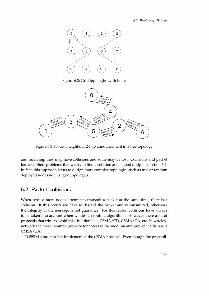
The second solution is based on sending and receiving messages from my one hopneighbours. First of all we will send a broadcast announcement message to advertiseall my one hop neighbours that I’m alive. After this, I know which are my neighboursand they know me due to the announcement message exchange. Now if I want to knowwhich are my n-hop neighbours I have to send a packet to my one hop neighbours withtwo information fields: a counter = n and a sender set to my ID node. When they receivedthe message, they decrease the counter in one unit and they will check if the counteris greater than 0. If it is, they will forward the message to its one hop neighbours. Inother case they will save the field sender as my n-hop neighbour. Figure 6.3 representsthe above.

The latter entails that depending on the how many n-hop neighbours we want tofind out, it may have a packet flooding. Because of a lot of packets are being sending

34

6.2 Packet collisions

Figure 6.2: Grid topologies with holes

Figure 6.3: Node 5 neighbour 2-hop announcement in a tree topology

and receiving, they may have collisions and some may be lost. Collisions and packetloss are others problems that we try to find a solution and a good design in section 6.2.In fact, this approach let us to design more complex topologies such as tree or randomdeployed nodes not just grid topologies.

6.2 Packet collisions

When two or more nodes attempt to transmit a packet at the same time, there is acollision. If this occurs we have to discard the packet and retransmitted, otherwisethe integrity of the message is not guarantee. For this reason collisions have alwaysto be taken into account when we design routing algorithms. However there a lot ofprotocols that tries to avoid this situation like: CSMA/CD, CSMA/CA, etc. In wirelessnetwork the most common protocol for access to the medium and prevent collisions isCMSA/CA.

TOSSIM simulator has implemented the CSMA protocol. Even though the probabil-

35

6 Design problems

ity for two nodes to start to transmit at the same time is very small, there is alwaysthat possibility. If this happen, the receiver will hear the overlap of the signals whichit’s almost certainly a corrupted packet. Because of that collisions can happen we needan extra mechanism to ensure that the packet arrives to the target properly. That is anacknowledgment extra message.

An acknowledgment is a packet sent to confirm that a message has come and more-over it has come correctly. With this feature if we don’t receive the ACK message in acertain time, we will retransmit the packet. TOSSIM has a component that implementthe ACK message. If we want to use it we have just to indicate when we send a messagethat we want the return ACK message from the receiver. On the other hand, if we waita while and we don’t receive the ACK we will retransmit the packet.

6.2.1 The broadcast ACK problem

The latter serves for all unicast packet, but what happens with the broadcast messages?If we broadcast a packet, we don’t know how many nodes the signal reach. Thus, wecan’t guess how many ACK we have to receive and also it’s impossible to know if wehave to relay the packet to a particular node. Hence, how can we ensure the integrityof a broadcast message?

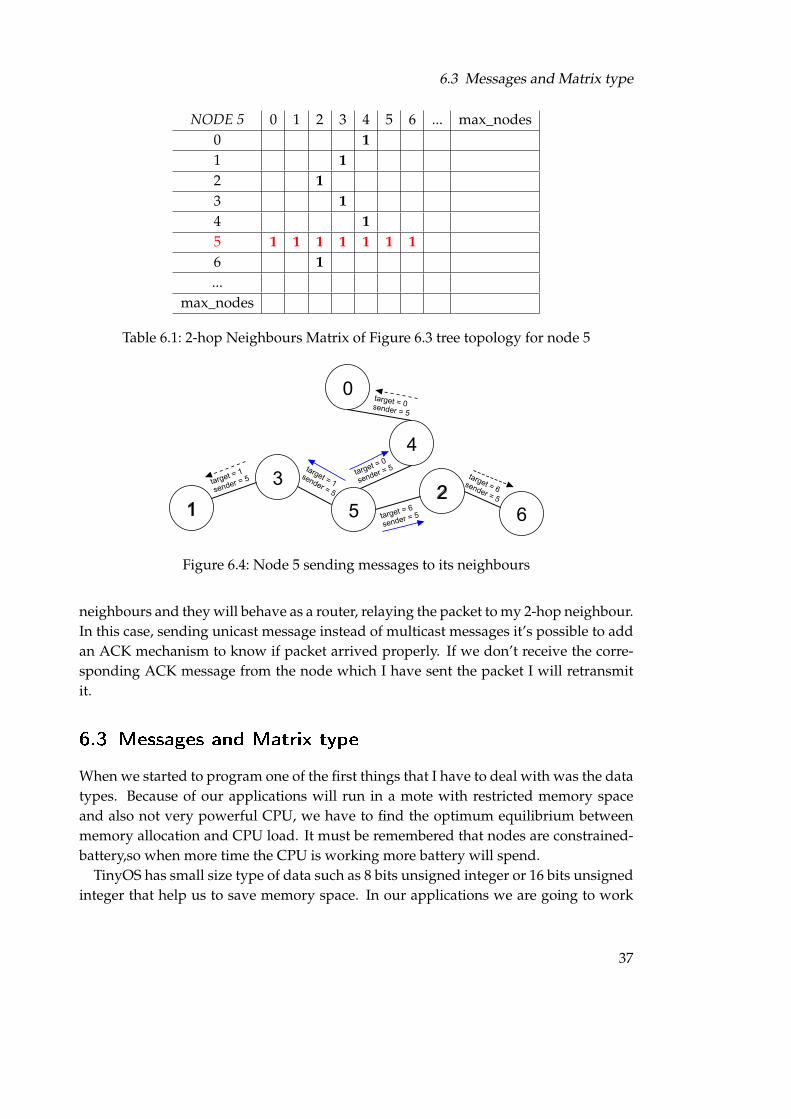
There is actually no mechanism to solve this. We will try to send the least possiblebroadcast message. Instead of this, each node will have neighbours matrix like Table6.1 representing all the information to reach a determinate node. For the tree topologyin figure 6.3, Table 6.1 shows all the information about my neighbours (in this case only2-hop neighbours). Red row indicates which are my neighbours (1 and 2-hop) and theothers rows point out which are my routers to reach the node index on the row. Forinstance to reach node 1 I have to rout the packet toward to node 3. Thereby if I want tosend a message to mote 6, we will find the router mote in row 6 set to 1 (that is node 2).So we will send a packet to node 2 telling that our target node is node 6. Then sensor 2

will look at its neighbour matrix which is the router to get node 6 (it is node 6). Figure 6.4also help us to understand this concept. Blue lines represent the first hop (first iteration)and dash lines are the second hop.

This table is built during the neighbours discovery process told before in section 6.1.1.Furthermore there are two points of view to allocate the data in the system. These areeither build it as a matrix bool type with maximum size sets as maximum nodes inthe network (an approximation) or build as a matrix integer type with size limit fixesto maximum number of neighboours per node. The matrix in Table 6.1 uses a booltype, however the advantages and disadvantages of those approach will be discussedat section 6.3.

Therefore, If we want to simulate a broadcast message and want to send a messageto all my 2-hop nodes, first of all we will send a message one per one to all my one-hop

36

6.3 Messages and Matrix type

NODE 5 0 1 2 3 4 5 6 ... max_nodes0 1

1 1

2 1

3 1

4 1

5 1 1 1 1 1 1 1

6 1

...max_nodes

Table 6.1: 2-hop Neighbours Matrix of Figure 6.3 tree topology for node 5

Figure 6.4: Node 5 sending messages to its neighbours

neighbours and they will behave as a router, relaying the packet to my 2-hop neighbour.In this case, sending unicast message instead of multicast messages it’s possible to addan ACK mechanism to know if packet arrived properly. If we don’t receive the corre-sponding ACK message from the node which I have sent the packet I will retransmitit.


When we started to program one of the first things that I have to deal with was the datatypes. Because of our applications will run in a mote with restricted memory spaceand also not very powerful CPU, we have to find the optimum equilibrium betweenmemory allocation and CPU load. It must be remembered that nodes are constrained-battery,so when more time the CPU is working more battery will spend.

TinyOS has small size type of data such as 8 bits unsigned integer or 16 bits unsignedinteger that help us to save memory space. In our applications we are going to work

37

6 Design problems

Node0 Node1 Node2 Node3 Node4 Node5 Node6 Node7 ... Max

Node0 0 1 0 1 1 0 0 0 ... 0

Node1 1 0 1 0 1 1 1 0 ... 0

Node2 0 1 0 1 0 1 1 1 ... 0

Node3 0 0 1 0 0 0 1 1 ... 0

Node4 1 1 0 0 0 1 0 0 ... 0

Node5 1 1 1 0 1 0 1 0 ... 0

Node6 0 1 1 1 0 1 1 1 ... 0

Node7 0 0 1 1 0 0 1 0 ... 0

Node 8 0 0 0 0 0 0 0 0 ... 0

.... ... ... ... ... ... ... ... ... ... 0

Max 0 0 0 0 0 0 0 0 ... 0

Table 6.2: Boolean Neighbor Matrix of grid network with 8 motes

with matrix to allocate some important information, so we have to take care to avoidwasting space. At this point we can find two different approaches: uses a booleanmatrix or integer matrix. The paragraphs below focuses on what are the advantagesand the drawbacks between uses an integer or a boolean matrix.

6.3.1 Boolean Matrix

Suppose that are network is build as a grid topology with 8 motes (Figure 3.1 repre-sents exactly the example). If we want to save in a matrix how are my neighbours wecan create a boolean matrix with the size equal to maximum number of nodes in thenetwork. Obviously in a real situation we don’t know the exact number of motes, butwe can make an approximation. Figure shows the neighbor matrix for all 8 nodes inthe grid network and variable Max defines the maximum number of nodes.

What are the advantages of this approach? The first big advantage is to know if node0 is connected with node 3 is very easy, just go to row 0 and column 3. The informationis always represented in the same way, thus searching in the neighbour matrix has aconstant (θ(1)) cost. Thereby the overload of the CPU is very small. In addition if wecompare the size needed in the memory to allocate this matrix is not very high due toboolean type is only one bit. Thus the latter matrix uses 64 bits (excluding how thememory is managed like alignments and so on).

However boolean matrix has also some drawbacks. The first is the size of the matrix.For instance if we are going to deploy a network with 500 nodes is not suitable to have amatrix of 500x500 (Max parameter would be five hundred). Furthermore to set matrix’slimit we need to know the number of nodes in the network and that is not viable.Besides, we are wasting memory space because of nodes usually don’t have more than

38


10 neighbours, and it means that to store which are my ten neighbours we are using 500bits. In addition, and this is a negative point to take into account, when we are sendingdata (like the neighbour list) the data field for the message in TinyOS doesn’t allow tosend more than 15 bytes. So for the example of 500 nodes we coudn’t send the neighborlist message because the data is too big. One solution to avoid that overflow is to sendonly the nodes that really are my neighbours (set to one in neighbour matrix), but if wedo this we are increasing to cost to send a message to θ(n). Thus, knowing that sendingmessage is a commonly operation, if at the end we are going to send just those nodeswhich are my neighbours, maybe it’s better to save only those neighbours in the matrix.The second approach is based on that and we will go into deep in the next subsection.

Moreover imagine that we want to send a message to all our neighbours. We knowthat TinyOS is a event driven system, so we can have a timer component that fires everyx milliseconds. Thereby, every time that the clock fires we can send a message to oneneighbours. For instance we want to node 0 send a message to all its neighbour. At thefirst timer fired, we check in the neighbour matrix (Table 6.2) if node 1 is my neighbourand if is, I will send a message. Suddenly in the next fired we will check if the nodeis connected with node 2 and if it is true, it will transmit a message. Later in the thirdfired we will look at node 3 and so on. We will repeat this process until the last vector’selement (in the example above the last node was five hundred). With this scenario wewill waste a lot of time (if the timer fired every 10 milliseconds, in the example we willuse 50 seconds just for sending one message to all my neighbours that maybe are onlyten).

At least but not at last, the nature of boolean type doesn’t make it suitable for storeall kind of data. Boolean is just a 0 or 1, and we need sometimes to store more complexinformation like which is the sender of the packet or what is the distance between twosensors. In this case only 1 bit is not sufficient and we must to resort to other data types.

6.3.2 Integer Matrix

Instead of having a matrix with all the nodes in the network, we are going to haveonly those which are my neighbours. The following table represents that solution for anetwork with 8 sensors.

The advantages of these solutions are several. First of all we are going to save inour matrix the nodes which are my neighbours. This allow us to reduce the memoryspace. Instead of having each node a field for all the nodes (500 bits per node in theprevious example), we are going to limit the size of the matrix to an approximationof how many neighbours per nodes we will have. As we said before, this maximumnumber of neighbours usually never exceeds ten. Consequently we are decreasing thematrix length, but we have to notice that now the vector type is integer. Bear in mindthat TinyOS has special types such as 8 bits unsigned integer, so we will declare the

39

6 Design problems

0 1 2 3 4 5 6 7 ... max_neighbours

Node0 1 4 5

Node1 0 2 4 5 6

Node2 1 3 5 6 7

Node3 2 6 7

Node4 0 1 5

Node5 0 1 2 4 6

Node6 1 2 3 5 7

Node7 2 3 6

...

max_neighbours

Table 6.3: Integer Neighbor Matrix of grid network with 8 motes

matrix as this type.Another advantage of this approach is that we can directly send a message of this

vector (is not necessary any conversion like in boolean matrix). If node 0 want to an-nounce which are its neighbors, it has just to send its list (that contains nodes 1,4 and5). This simplifies the sending and the cost of that is θ(1). However if we want to knowif the node 5 is a neighbour of 0, we have to go through all the vector position per po-sition and do the comparison (θ(n)). This is a clear disadvantage due to this kind ofcomparison is a taks that often happens.

6.3.3 The solution adopted

As in a lot of other things happens, the best solution is not black or white, sometimesthe best choice is a mix between both. That is exactly what we will do. For somepurpose it’s better the boolean matrix, and in other cases integer approach is better.Thus depending on which kind of data we are going to store and which operation arewe going to execute more times will choose one type or the other. For example for theneighbor matrix (as we can see in Table 6.1) it’s very easy to check if a determinate nodeis my neighbours. But realistic situation we are going to send packets only to our one-hop neighbours as the in Figure 6.4. Consequently it’s better to have an integer vectorwith my one-hop neighbours (we will discuss this further on in section 6.4) because thisvector is shorter and more compact and will allow us don’t waste too many clock ticks.

However as we mentioned before, in some cases boolean type can’t store all the datathat we receive (we need a more appropriate type of data like integer) and it is betterthe integer matrix. In addition sometimes it’s better to have integer vectors (they havea more compact information), otherwise we will waste a lot of time doing nothing.

40

6.4 Synchronization

6.4 Synchronization

In all distributed system synchronization is a big problem that all the programmershave to deal with. In this section we will not address the issue of how to sincrhonizatethe nodes with the others when they start to run in the network (there are many algo-rithms that allows a new node to synchronized with the system). In these paragraphswe will be aware of the importance of don’t desyncrhonizate during the program exe-cution.

If we are running the network in the simulator, we haven’t got any problem to syn-chronized the nodes at the beginning because TOSSIM help us to this task. The thingwould be worse if we deploy the network in a real enviorment, but we are going tofocus only if we use the simulator.

The main task of all nodes are sending and receiving. Because we are interested onlyin sending packets to our fist hop neighbor (then those will relay the message to thetarget node), the vector that we will access more often will be the one-hop neighbor list.That seems like this:

Node 0 1 4 ...Node 1 0 2 5 ...Node 5 1 4 5 6 ...Node 11 7 10 ...

0 1 2 3 4 ... max_neighbours

Table 6.4: One-hop neighbour list of several nodes in a grid topology (Figure 6.1)

Let’s take an example to show what happens if the sensors are not syncrhonizated.In any algorithm when a new round starts, it’s common at the beginning to send somemessages to our neighbours. Thus, in each time that clock fired, we will transmit apacket to one node. In the first fired we send to the node located at position 0. In nextalarm fired we will transmit to the node at position 1 in the vector and so on. Therebywe can realize that there are nodes (like 1 or 11) that have to wait doing nothing untiltimer counter arrives to max_neighbours. Regardless we are wasting time we are forcedto wait, otherwise some nodes could preempt others and data structures might not beconsistent.

We must not lost the sight of the fact that max_neighbour is a critical parameter. If wedefine that parameter too large, the most part of the time nodes will be idle. For instancejust for sending an announcement to all my neighbours if we set max_neighbours equalto 30 and the timer fires every 100 milliseconds we will spend 3 seconds to send onlyone packet to all my one-hop neighours. On the contrary if the parameter is too low (forexample fixed to 3), and we have more neighbours than this value, we can’t allocate thedata of all motes.

41

6 Design problems

To sum it up all nodes have to keep syncrhonizated, despite of that means that theyare wasting time. This can be minimized adjusting the critical parameter max_neighbours.

6.5 Fragmentation

Our TinyOS header field each packet has the following fields: type of message, sourceof message, packet sequence number, number of fragment and data. For each of thesefields we can use 1 Byte and it will be enough (255 is the largest value because the datatype is unsigned integer), except for source field, which the TinyOS standard says thatthe default type of data is an unsigned integer of 16 bits (2Bytes or what is the same65535 possibles nodes in the network). If we sum up all the required values we have aheader of 5 Bytes.

In TinyOS the maximum data payload is 28 Bytes, so for the data we only have 23Bytes left. If this were not enough, we need a two dimensional vector in the data fieldwhere the first dimension denotes the node ID and the second the information attachedto the node. Besides the type of data of this vector has to be again an unsigned integerof 16 bits. Thus if we had 23 Bytes for data, now we have to divided it by two due tothe two dimensional vector and at the end we have only 11 Bytes. This entails that wecan only allocate 5 memory locations of 2 Bytes. The Figure 6.5 will represent all theheader fields and its corresponding size.

Figure 6.5: Header fields and sizes

The standard MAC that TinyOS includes doesn’t support fragmentation. It has beendevelopment another MAC for TinyOS that support fragmentation and more advancedfeatures such as s-mac or t-mac. In our case, we are going to keep the predefined MACand we will calculate by hand how many packet we will need and we will send them.As we have seen above, if the data is quite large we will need several fragments butif the number of fragments it too high our algorithm will take a long time to finishbecause it has to transmit a lot messages. To figure out these problem we can compressthe data before sending the packet. These solution will be explained in the Section 6.6.

42

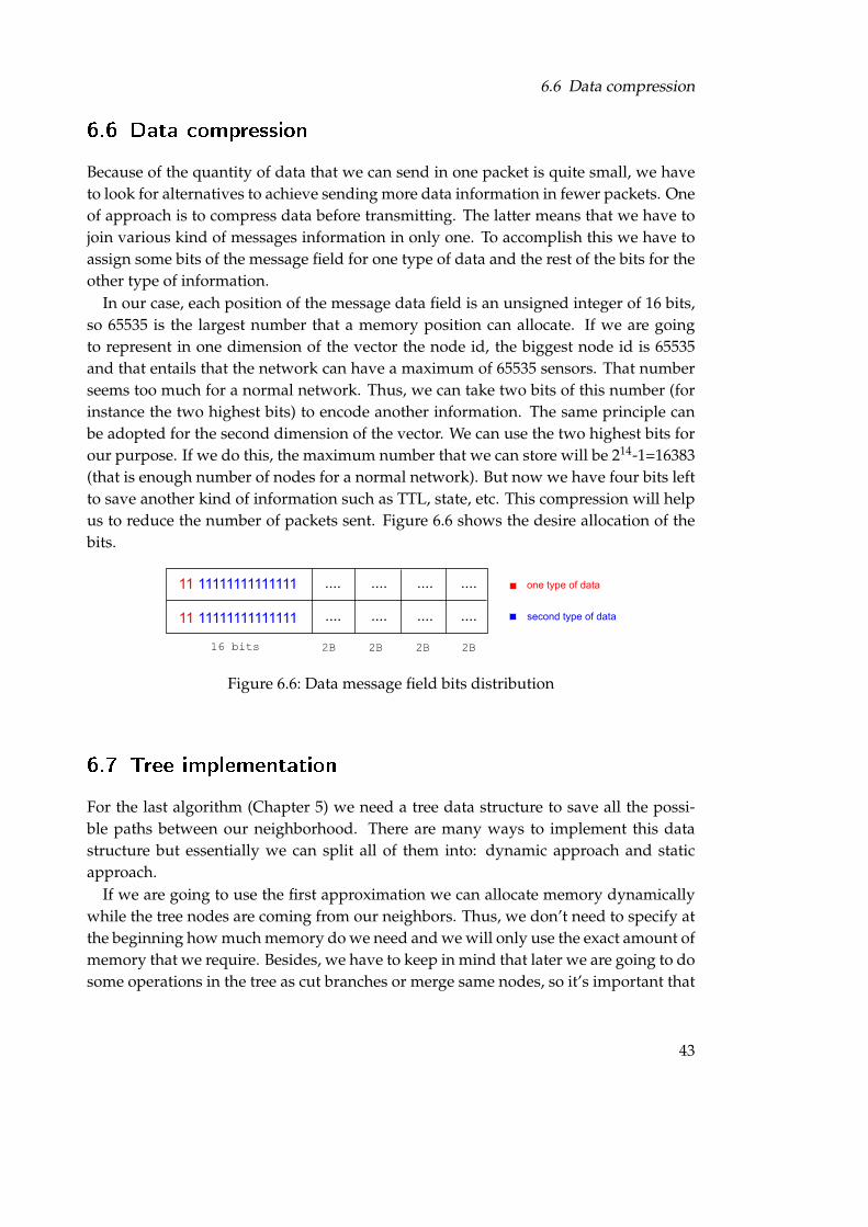
6.6 Data compression

6.6 Data compression

Because of the quantity of data that we can send in one packet is quite small, we haveto look for alternatives to achieve sending more data information in fewer packets. Oneof approach is to compress data before transmitting. The latter means that we have tojoin various kind of messages information in only one. To accomplish this we have toassign some bits of the message field for one type of data and the rest of the bits for theother type of information.

In our case, each position of the message data field is an unsigned integer of 16 bits,so 65535 is the largest number that a memory position can allocate. If we are goingto represent in one dimension of the vector the node id, the biggest node id is 65535and that entails that the network can have a maximum of 65535 sensors. That numberseems too much for a normal network. Thus, we can take two bits of this number (forinstance the two highest bits) to encode another information. The same principle canbe adopted for the second dimension of the vector. We can use the two highest bits forour purpose. If we do this, the maximum number that we can store will be 214-1=16383(that is enough number of nodes for a normal network). But now we have four bits leftto save another kind of information such as TTL, state, etc. This compression will helpus to reduce the number of packets sent. Figure 6.6 shows the desire allocation of thebits.

Figure 6.6: Data message field bits distribution

6.7 Tree implementation

For the last algorithm (Chapter 5) we need a tree data structure to save all the possi-ble paths between our neighborhood. There are many ways to implement this datastructure but essentially we can split all of them into: dynamic approach and staticapproach.

If we are going to use the first approximation we can allocate memory dynamicallywhile the tree nodes are coming from our neighbors. Thus, we don’t need to specify atthe beginning how much memory do we need and we will only use the exact amount ofmemory that we require. Besides, we have to keep in mind that later we are going to dosome operations in the tree as cut branches or merge same nodes, so it’s important that

43

6 Design problems

the complexity of these operations don’t be so high. With a pointer tree implementationsome of these function could be done easily with a good cost. In spite of all thoseadvantages, TinyOS discourages dynamic memory. The reason is that TinyOS stackdoesn’t have space for heap and even thought that is possible to compile a code withdynamic memory, it is very dangerous because in any moment could be an overflow.

The second approach is to use static memory. TinyOS handles it very good, but it’sless intuitive for a tree implementation and also you have to define first how muchmemory are you going to allocate. This could be a parameter in the header file, but youhave to fix it properly otherwise the algorithm will not work accurately.

Figure 6.7: Dynamic representation: left son pointer, right brother pointer and node id.

In our algorithm because we can’t use dynamic memory in TinyOS, we are going touse static memory but using the pointers representation. In dynamic memory a goodrepresentation of a node could be a left son right brother representation That is: a leftpointer to the our son, a right pointer to our brother, and the node Id (see Figure 6.7).Thus, if we want to do the same but in static memory we need a three dimensions arraywhere:

• First dimension: allocate the node Id.

• Second dimension: save the index of our son.

• Third dimension: save the index of our brother.

With these model we can port the pointers idea to a static memory allocation. Thenext illustrations will help us to understand better our idea. If we have the networkof the Figure 6.8 and we want to know the three hop neighborhood (without repeatnodes) we will get the right part of the Figure 6.8. If we represent the tree with thepointer structure we will get the memory representation of the Figure 6.7 meanwhile ifyou chose the static design we will have the Figure 6.9. If we compare both solutionsare equals.

44

6.7 Tree implementation

Figure 6.8: Example of network (left part) and the 3-hop of node 8 neighborhood repre-sented by a tree (right part)

node Id 8 16 12 19 12 16 2 24 24 2 ...left son 1 4 5 6 - - 8 9 - - ...right brother - 2 3 3 - - 7 7 - - ....

0 1 2 3 4 5 6 7 8 9 ... max_tree

Figure 6.9: Static representation of the Figure 6.8

node 16 node 12 node 19 node 8 neighborhood treehop 1 16 12 19 8{16,12,19}hop 2 12,8 8,16 8,2,24 8{16{12},12{16},19{24,2}}hop 3 8,19,12 8,19,2,24 16,12,24,2 8{16{12},12{16},19{24{2},2{24}}}

Table 6.5: Tree transmissions for node 8

Another important issues is how to transmit the tree information to our neighbors.He have to remember that in each packet we only have space for the data of 5 nodes(check Figure 6.5). Hence instead of sending every time the whole tree that we havereceived to our neighbor, we just send the new nodes that collect. Table 6.5 illustrates acomplete round for the node 5 and at the end as we can see the tree that we finally getis the same as in Figure 6.8, Figure 6.7 (dynamic representation) and Figure 6.9 (staticrepresentation).

45

6 Design problems

46

7 Security Analisys

Security is an important issue for WSN by the fact that they can be set up in criticalsystems like airports or hospitals, burglar alarms, military applications, enviormentcontrol or monitoring any kind of activity. Even thought their constraints limit ourcapacities to add the classic security mechanisms to the sensors hardware and software,we have to come up with new techniques to avoid an intruder to steal or manipulatethe data that could cause a disaster.

The goals of the any secure system is to provide confidentiality, integrity and avail-ability (CIA) for the data, protecting information from unauthorized access, use, disclo-sure, disruption, modification or destruction [1]. Cryptographic functions are usuallyused to assure these, but because of lack of memory and power in the sensors, most ofthese approaches can not be converted directly from the traditional security systems toWSN. Besides as happened in the early days of Internet, WSN clustering protocols arenot designed for security and they are insecure.

Thus we have to think new mechanisms to add a security layer to our sensors. Someresearches have been studying this issues and they have already implemented crypto-graphic methods. For example, TinyOS 1.0 has a module called TinySec that provide alink layer security architecture. If we are using the new TinyOS 2.0 or 2.1, few monthago a new implementation for AES have been developed for MICAz over TinyOS. Butthe problem is that for TOSSIM there is not any HAL on the simulator to emulate thebehavior of the cryptographic module.

In the next sections we will study which are the most common attacks for a WSN andhow can these threats be used against the algorithms described in before chapters.

7.1 Attacks in WSN

Security attacks can be split into two big categories: passive and active. In a passive at-tack the intruder does not transmit anything to try to confuse the network, it just standand listen what the other are sending. This kind of attack try to break the confidential-ity premise, because it is listening a conversation that is not addressed to him. On theother hand, with the active attacks malicious transmit something in other to corrupt thenormal operation of the network and nodes. This kind of attacks are more dangerousand can endanger the confidentiality, the integrity and the availability of the nodes.

47

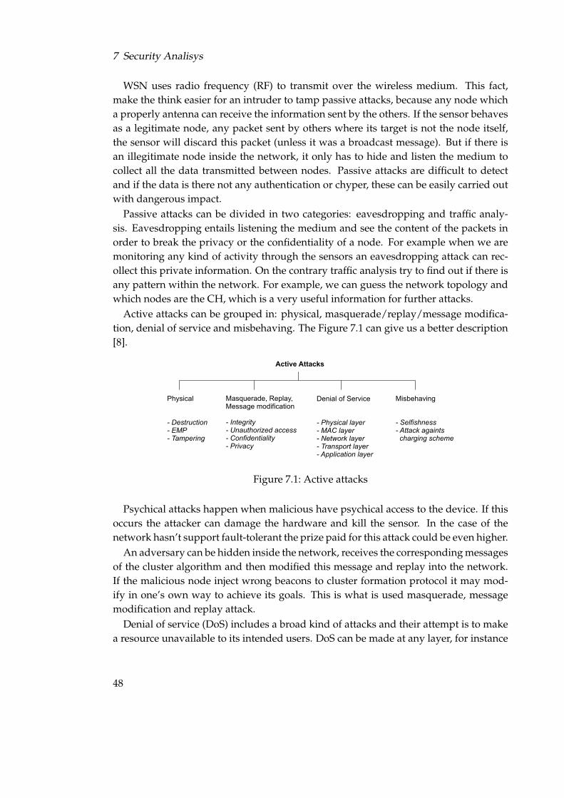
7 Security Analisys

WSN uses radio frequency (RF) to transmit over the wireless medium. This fact,make the think easier for an intruder to tamp passive attacks, because any node whicha properly antenna can receive the information sent by the others. If the sensor behavesas a legitimate node, any packet sent by others where its target is not the node itself,the sensor will discard this packet (unless it was a broadcast message). But if there isan illegitimate node inside the network, it only has to hide and listen the medium tocollect all the data transmitted between nodes. Passive attacks are difficult to detectand if the data is there not any authentication or chyper, these can be easily carried outwith dangerous impact.

Passive attacks can be divided in two categories: eavesdropping and traffic analy-sis. Eavesdropping entails listening the medium and see the content of the packets inorder to break the privacy or the confidentiality of a node. For example when we aremonitoring any kind of activity through the sensors an eavesdropping attack can rec-ollect this private information. On the contrary traffic analysis try to find out if there isany pattern within the network. For example, we can guess the network topology andwhich nodes are the CH, which is a very useful information for further attacks.

Active attacks can be grouped in: physical, masquerade/replay/message modifica-tion, denial of service and misbehaving. The Figure 7.1 can give us a better description[8].

Figure 7.1: Active attacks

Psychical attacks happen when malicious have psychical access to the device. If thisoccurs the attacker can damage the hardware and kill the sensor. In the case of thenetwork hasn’t support fault-tolerant the prize paid for this attack could be even higher.

An adversary can be hidden inside the network, receives the corresponding messagesof the cluster algorithm and then modified this message and replay into the network.If the malicious node inject wrong beacons to cluster formation protocol it may mod-ify in one’s own way to achieve its goals. This is what is used masquerade, messagemodification and replay attack.

Denial of service (DoS) includes a broad kind of attacks and their attempt is to makea resource unavailable to its intended users. DoS can be made at any layer, for instance

48

7.2 Security threats in TinyOS

at psychical layer we can cause DoS in a sensor with just emit another signal with thesame frequency near the node. This will cause a lot of noise in the carrier, so the re-ceiver node can not receive the information properly. In the link layer various DoS canbe done successful depending on the medium access control (MAC) that the sensorshave implemented. MAC for TinyOS is just CSMA, unlike Wifi standard (802.11b/g)uses CSMA/CA and RTS/CTS packets to solve the problem of hidden terminals andexposed terminals. Regarding RTS/CTS is not available in TinyOS the problem of thehidden terminal is always present. Thus a node A that is ready to transmit will trans-mit to node B because he does not see the malicious terminal C (according to CSMA)and the C sensor can be transmitting always and cause a collisions in node B, so node Bwill never receive the signal of A. In this case, the node C will have the resource (nodeB) always for him, meanwhile node A can never get the source. This latter behaviorcan also be included as misbehaving category. Furthermore the continuous retransmis-sions of the packet for node A can also deplete the node battery. In the network layerwhere clustering algorithms work a illegitimate node can refuse message or alter it tonot follow the algorithm and avoid node to communicates with others and form prop-erly clusters. Finally at the transport layer the ACK mechanism and messages can bemanipulated to jam some nodes.

We should also mention that we can have two different kind of attackers: node-attacker and laptop-attacker. The last one has more powerful hardware, so they havemore battery, more CPU resources, more memory and best antenna which can reachfurther distances than a normal mote. All of these advantages against the nodes, makelaptop-attacker very hazardous for our network.

7.2 Security threats in TinyOS

TinyOS is very vulnerably to the attacks at layer 1 and 2. At layer 1 an intruder mightjam a carrier just only transmitting a signal at the same frequency near the victim node.This jam cause a DoS in the victim. In this case, TinyOS in not guilty, because the break-down is due to physics issues more than the way that the operative systems managesthe resources. Hence this attack at layer 1 will works in all WSN with any OS. How-ever at layer 2, TinyOS has a implementation of the MAC protocol that is very easy tocollapse. As we discuss in the above section the OS uses only CSMA to access to themedium which leads us a possible scene with the hidden terminal problem. A malignsensor C that node A doesn’t see can transmit data to node B on purpose originatingthat node B doesn’t receive the message from A properly due to the noise between bothsignal (A and C). This situation can be avoided using RTS/CTS messages, but becausea good reasons TinyOS doesn’t adopt them.

Another layer that can be attacked is the transport layer. We can use ACK mechanism

49

7 Security Analisys

to assure that a unicast packet has been received in the target a node. But it might bea double-edged sword for our cluster algorithm, because if some node try to send amessage to another node and this doesn’t answer after X tries (this means that doesn’treceive the ACK) the node will be remove from the neighbor list (the node looks like beshutdown). Thus, we can make some noise in the node to not let him to reply with theACK message and after a while this node will be isolate from the network (all neighborswill have delete it from the neighbor list).

7.3 LEACH Algorithm

LEACH algorithm was described in Chapter 2, therefore here we are going to analyzewhich are the security threats and possible attacks to carry out only in the networklayer (the clustering algorithm itself).

7.3.1 HELLO �ood attack

In LEACH algorithm once the CHs have been chosen based on a probabilistic formula,they have to send a broadcast message to all its neighbors. Then the non-CH nodes haveto associate to only one CH based on some discriminatory parameter as strength signal,distance or battery level. LEACH original algorithm chooses the CH with best signalstrength. This fact can lead to a malicious (a laptop-attacker with a power antenna) toemit always a strength signal which is best than any node. Thus every sensor in thenetwork, will try to associate to this node. However not all motes will associate withthe intruder, because the radio signal is not as powerful as a laptop and they can’t reachthe adversary node. These lost packets may involve the network to stay in a inconsientstate. In other words, the malicious has caused a DoS.

In our own implementation, we don’t use the strength signal to associate to the bestnode. Instead of these, but we use as a discriminatory factor the distance. Because ofour motes are placed on a fix grill (we know which are the distance between the nodes)consequently HELLO attack could not been carried out. On the other hand this fixedtopology don’t give us flexibility to design our own networks.

7.3.2 Sybil attack

Another choice instead of causing a DoS is to deploy strategical malicious nodes inorder to forward all the data in the network to our illegitimate motes. This can easybe countered for the matter that LEACH chooses in each round a CH that has not be-ing chosen previously. In this scenario is when Sybil attack comes up. In Sybil attacka single node presents multiple identities [10]. Thus, the adversary can every roundchanges its identity to appear as a new node for the rest of the network, consequently it

50

7.4 Distributed cluster (Clique) Algorithm

can be chosen again. We can forward all the data from the network to our sensors andthen analyze the traffic which is in plain text or make a wormhole to reply the data inanother point.

7.3.3 Other attacks

Our LEACH implementation has been developed thinking always that the algorithmis going to be used in the right way. As a consequence of that if the nodes don’t followthe normal flow of the algorithm it may drive the network to a inconsistent state. Forexample, if we have an adversary that is a CH and receive all the data from its childrenbut doesn’t send the data aggregation to the sink, this will be waiting until they receivethe package from all the CH (causing a DoS).

Another choice is to send messages like associate when is not it right time in the al-gorithm flow. In case of the associative messages, each packet that the CH receives willallocate slot in the TDMA shadily for the received node, without checking if the nodeis already in the schedule. If the malicious node send a burst of associative messages,these can lead to a buffer overflow (of the TDMA schedule vector). Even if the algo-rithm checks for no redundant nodes in the TDMA timetable, the adversary can alwaysuses the Sybil attack to change its identity.

7.4 Distributed cluster (Clique) Algorithm

The distributed cluster formation protocol tries to build consistent clusters after foursteps. In each of these steps every node relies on its neighbors tell the true, so at theend they can achieve a common, unique and consistent clique. However if in any of thefour phases (see Section 3.2) a malicious inject wrong data, the cluster formation couldbe altered.

7.4.1 Silence attack

A node which is communicating with a node but keep silence with another one is mak-ing a silence attack. In this type of clustering formation this attack can be very dan-gerous because introduces inconsistency between nodes. At this point, we are going tointroduce a new factor: malicious node could have a directional antenna, so they cansend message to a desire direction.

In the step 1 of the algorithm an adversary can send announcement message to oneneighbor, but be mute to another. This fact, could cause inconsistencies between bothneighbors. In our algorithm because of step 2 we order the local maximum clique re-ceived, we can chose another clique despite of a node is not in our neighbor list. Hencethis attack in this phase will not affect to the network.

51

7 Security Analisys

But in the step 2 the attack can cause several troubles. Illegitimate nodes can sendmodified local maximum clique to two of his neighbors two introduce inconsistencybetween them. For example if node C (malicious) sends to A (normal node) a betterclique that includes A and B (normal node), but keep silence and doesn’t send the samemessage to B, then node A will update its clique to the best clique sent by node C.However node B hasn’t received this better clique. Thus imagine that B has update itsbest clique as the set received by A, but actually mote A best clique is the set receivedby C (which is different from the clique received by B). As we can see this attack cancause inconsistency between two nodes and brakedown the algorithm in next steps.

In the phase each nodes transmit each updated clique to its neighbors. For everynode in the final clique list, the sensor check if that node also include me in the list. Inothers words, nodes must be mutually in both list. As a result of this, a node can addsome troubles by sending a modified clique to one node and withhold the message toanother.

7.4.2 HELLO, Sybil and Wormhole attacks

Clique algorithm is also sensitive to HELLO attack. Think about a scenario when amalicious node has ID equal to 0 (we can use Sybil attack to achieve this) and then itsends a very powerful signal (from a laptop) that reach all the nodes. Consequently allnodes will include the attacker mote in its neighbor list. For the next phase, the intrudercan also create a fake local maximum clique very large to ensure that it will be chosenas the best clique. Moreover this attack could be combined with placed strategicallynodes in order to have at least one malicious node in each cluster and then forward thedata with a wormhole or just keep it for analyze.

7.5 Distributed bounded-distance multi-clusterhead

algorithm

Spohn-Garcia is a clusted based and this fact entails that the protocol is vulnerable tothe same attacks as the distributed cluster (clique) protocol. Nevertheless there is a spe-cial attack that we have to remark because it’s endanger in this protocol: the selectiveforwarding attack.

7.5.1 Selective forwarding

As we show in the Section 4.2 the formation algorithm is divided in two phases. Duringthe step 1 all nodes have to discover which are their neighbors and later depends onthe neighbor list set their status. An evil node can forward the information received

52

7.6 New Distributed multi-clusterhead algorithm

not to all its neighbor and make the victim node to believe that it is not linked to moreneighbors. This action can make the cheated sensor to become as a CH node.

In the phase two if the neighborhood doesn’t have data consistency between them,it can be a real mesh. One node A could think that it has sent a message to node B,when could be not true if the malicious mote that is in the halfway doesn’t forward itto node B. Moreover if a node that has been converted in CH sent the NA packet (tonotify its neighbors that it a dominated node) doesn’t arrive to its target the addressednode never will know that the status of the node has changed. The same could appliedfor the notification messages (that tell a node that it has to convert in CH). The resultof these can be that the number of CH can increase because nodes don’t have all theinformation and messages from their neighbors.

7.5.2 Others attacks

As we said before Spohn-Garcia protocol is exposed to identical threads as the cliquealgorithm. A intruder node can accomplish a Sybil attack and set it’s Id to 0 (the lowestId the better it is, because in case of there are more validated CH than the parameter k

in our list within the same distance, we will chose k lowest ID). After this, a node couldsend a NA message declaring itself as a CH. All nodes will add him at the validates CHlist and at the end of the algorithm is it likely to be chosen as CH.

7.6 New Distributed multi-clusterhead algorithm

During the analysis of the previous algorithms we have seen a lot of attacks that can becarried out. In this new protocol all of these attacks can also be performed. Moreoverwe can look into the code to see which parts are more vulnerable.

One of the points that we can exploit in the protocol is the fact that each neighbornode has to allow a head that is attempting to escape. If a malicious sensor doesn’tlet any of their nodes to escape the number of CH in the network could increase a lot.Besides if we send join messages to all the neighborhood they will become head everysensor.

7.7 Conclusions

Through this chapter we have seen that any kind of attack is easy to carry out witha very dangerous consequences. To prevent these threads the best and effective solu-tion is to make a message authentication for unicast and broadcast message and add akey management protocol to authenticate all sensors against the base station. To fulfillthis requirements researching have been investigating and nowadays there are some

53

7 Security Analisys

alternatives for processors with 8-bits to accomplish this. Maybe security is not as scal-able as in other security systems, but the challenge is to think about and develop newsecurity mechanism adjusted for WSN.

54

Bibliography

[1] Information security. http://en.wikipedia.org/wiki/Information_security.

[2] Micaz datasheet. http://www.xbow.com/Products/Product_pdf_files/

Wireless_pdf/MICAZ_Datasheet.pdf.

[3] Tinyos. http://en.wikipedia.org/wiki/TinyOS.

[4] Tinyos community forum. http://www.tinyos.net/.

[5] Tinyos mail list. [email protected].

[6] Tinyos tutorials. http://docs.tinyos.net/index.php/TinyOS_Tutorials.

[7] Ameer Ahmed Abbasi and Mohamed Younis. A survey on clustering algotihmsfor wireless sensor networks. Elsevier, 2007.

[8] Erdal Cayirci and Chunming Rong. Security in Wireless Ad Hoc and Sensor Networks.2009.

[9] Y.P. Chen, A.L. Liestman, and J. Lui. Ad hoc and sensor networks. Nova Science

Publisher, Chapter 4: Clustering agorithms for ad hoc wireless networks, 2004.

[10] J. R. Douceur. The sybil attack. 1st International Workshop on Peer-to-Peer Systems,2002.

[11] David Gay, Philip Levis, Robert von Behren, Matt Welsh, Eric Brewer, and DavidCuller. The nesc languaje: A holistic approach to networked embedded systems.

[12] Weisong Shi John Paul Walters, Zhengqiang Liang and Vipin Chaudhary. Wirelesssensor network security: A survey. 2006.

[13] Sophia Kaplantzis. Security models for wireless sensor networks. Master’s thesis,2006.

[14] Holger Karl and Andreas Willig. Protocols and Architectures for Wireless Sensor Net-

works. 2005.

[15] Chris Karlof and David Wagner. Secure routing in wireless sensor networks: at-tacks and countermeasures. Elsevier, 2003.

55

Bibliography

[16] Turgay Korkmaz. Tinyos and nesc programming. http://www.cs.utsa.edu/

~korkmaz/teaching/cn-resources/tinyos/basictinyos2.ppt, Spring 2009.

[17] Philip Levis. TinyOS programming. October 2006.

[18] David Moss. Introduction to TinyOS 2.x.

[19] Marco Aurélio Spohn and J.J. Garcia-Luna-Aceves. Bounded-distance multi-clusterhead formation in wireless ad hoc networks. Elsevier, 2006.

[20] Kun Sun, Pai Peng, Peng Ning, and Cliff Wang. Secure distributed cluster forma-tion in wireless sensor networks. University Daily Kansan.

[21] Yang Li-zhen Wang Xiao-yun and Chen Ke-fei. Sleach: Secure low-energy adapta-tive clustering hierarchy protocol for wireless sensor networks. WUJNS, 2005.

56

clustering algorithms for wireless sensor networks and security

Documents