clustering basic concepts and algorithms 2courses.washington.edu/css581/lecture_slides/12... ·...
TRANSCRIPT

Jeff Howbert Introduction to Machine Learning Winter 2014 1
Clustering
Basic Concepts and Algorithms 2

Jeff Howbert Introduction to Machine Learning Winter 2014 2
Hierarchical clustering
Density-based clustering
Cluster validity
Clustering topics
Jeff Howbert Introduction to Machine Learning Winter 2014 3
Proximity is a generic term that refers to either similarity or dissimilarity.Similarity
– Numerical measure of how alike two data objects are.– Measure is higher when objects are more alike.– Often falls in the range [ 0, 1 ].
Dissimilarity– Numerical measure of how different two data objects are.– Measure is lower when objects are more alike.– Minimum dissimilarity often 0, upper limit varies.– Distance sometimes used as a synonym, usually for specific
classes of dissimilarities.
Proximity measures

Jeff Howbert Introduction to Machine Learning Winter 2014 4
A clustering is a set of clusters
Important distinction between hierarchical and partitional clustering– Partitional: data points divided into finite
number of partitions (non-overlapping subsets)each data point is assigned to exactly one subset
– Hierarchical: data points placed into a set of nested clusters, organized into a hierarchical tree
tree expresses a continuum of similarities and clustering
Approaches to clustering

Jeff Howbert Introduction to Machine Learning Winter 2014 5
Produces a set of nested clusters organized as a hierarchical treeCan be visualized as a dendrogram– A tree like diagram that records the sequence
of merges or splits
Hierarchical clustering
1 3 2 5 4 60
0.05
0.1
0.15
0.2
1
2
3
4
5
6
1
23 4
5
Jeff Howbert Introduction to Machine Learning Winter 2014 6
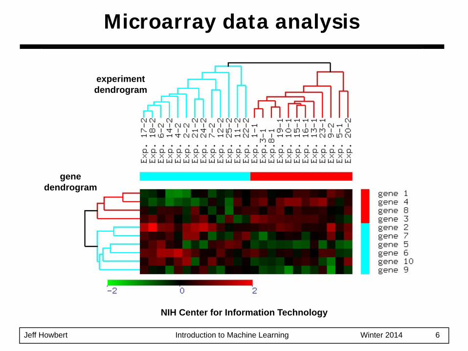
Microarray data analysis
NIH Center for Information Technology
experimentdendrogram
genedendrogram

Jeff Howbert Introduction to Machine Learning Winter 2014 7
Melanoma gene expression profiles
Univ. of Maryland, Human-Computer Interaction Lab

Jeff Howbert Introduction to Machine Learning Winter 2014 8
Genetic distance among wheat cultivars
Hierarchical clustering based on 13 quality traits of 75 wheat landraces including seven wheat cultivars.
Australian Society of Agronomy, The Regional Institute Ltd.
Jeff Howbert Introduction to Machine Learning Winter 2014 9
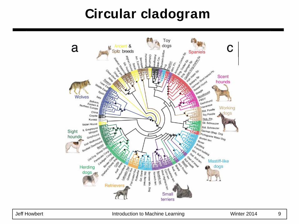
Circular cladogram
Jeff Howbert Introduction to Machine Learning Winter 2014 10
Do not have to assume any particular number of clusters– Any desired number of clusters can be
obtained by ‘cutting’ the dendogram at the proper level
They may correspond to meaningful taxonomies– Example in biological sciences (e.g., animal
kingdom, phylogeny reconstruction, …)
Strengths of hierarchical clustering
Jeff Howbert Introduction to Machine Learning Winter 2014 11
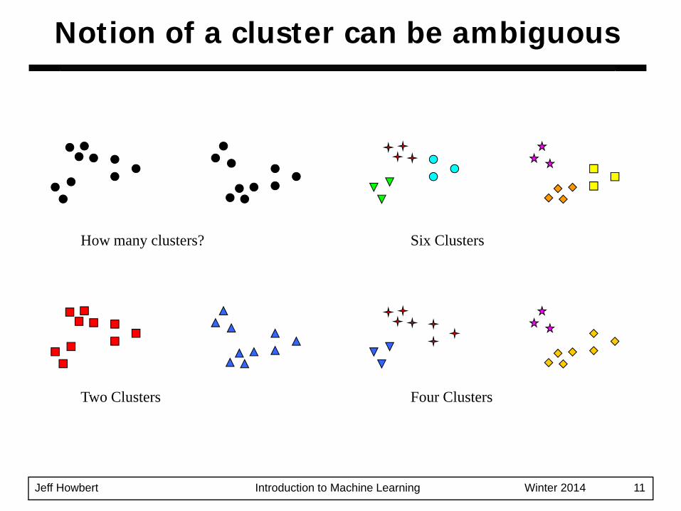
Notion of a cluster can be ambiguous
How many clusters?
Four ClustersTwo Clusters
Six Clusters
Jeff Howbert Introduction to Machine Learning Winter 2014 12
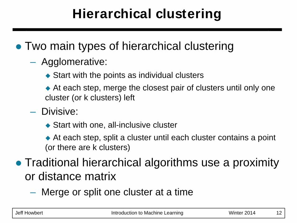
Two main types of hierarchical clustering– Agglomerative:
Start with the points as individual clustersAt each step, merge the closest pair of clusters until only one
cluster (or k clusters) left
– Divisive: Start with one, all-inclusive cluster At each step, split a cluster until each cluster contains a point
(or there are k clusters)
Traditional hierarchical algorithms use a proximity or distance matrix– Merge or split one cluster at a time
Hierarchical clustering

Jeff Howbert Introduction to Machine Learning Winter 2014 13
More popular hierarchical clustering techniqueBasic algorithm is straightforward
1. Compute the proximity matrix2. Let each data point be a cluster3. Repeat4. Merge the two closest clusters5. Update the proximity matrix6. Until only a single cluster remains
Key operation is the computation of proximities between cluster pairs
– Different approaches to defining the distance between clusters distinguish the different algorithms
Agglomerative clustering algorithm

Jeff Howbert Introduction to Machine Learning Winter 2014 14
Starting situation
Start with clusters of individual points and a proximity matrix
p1
p3
p5
p4
p2
p1 p2 p3 p4 p5 . . .
.
.
. proximity matrix
Jeff Howbert Introduction to Machine Learning Winter 2014 15
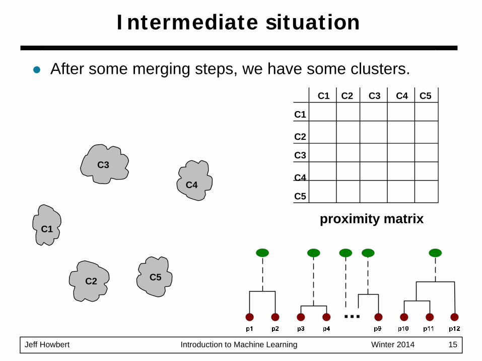
Intermediate situation
After some merging steps, we have some clusters.
C1
C4
C2 C5
C3
C2C1
C1
C3
C5
C4
C2
C3 C4 C5
proximity matrix

Jeff Howbert Introduction to Machine Learning Winter 2014 16
Intermediate situation
We decide to merge the two closest clusters (C2 and C5) and update the proximity matrix.
C1
C4
C2 C5
C3
C2C1
C1
C3
C5
C4
C2
C3 C4 C5
proximity matrix

Jeff Howbert Introduction to Machine Learning Winter 2014 17
After merging
The question is “How do we update the proximity matrix?”
C1
C4
C2 U C5
C3? ? ? ?
?
?
?
C2 U C5C1
C1
C3
C4
C2 U C5
C3 C4
proximity matrix

Jeff Howbert Introduction to Machine Learning Winter 2014 18
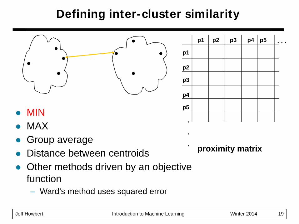
Defining inter-cluster similarity
p1
p3
p5
p4
p2
p1 p2 p3 p4 p5 . . .
.
.
.
similarity?
MINMAXGroup averageDistance between centroidsOther methods driven by an objective function– Ward’s method uses squared error
proximity matrix
Jeff Howbert Introduction to Machine Learning Winter 2014 19
p1
p3
p5
p4
p2
p1 p2 p3 p4 p5 . . .
.
.
. proximity matrix
MINMAXGroup averageDistance between centroidsOther methods driven by an objective function– Ward’s method uses squared error
Defining inter-cluster similarity

Jeff Howbert Introduction to Machine Learning Winter 2014 20
p1
p3
p5
p4
p2
p1 p2 p3 p4 p5 . . .
.
.
. proximity matrix
MINMAXGroup averageDistance between centroidsOther methods driven by an objective function– Ward’s method uses squared error
Defining inter-cluster similarity

Jeff Howbert Introduction to Machine Learning Winter 2014 21
p1
p3
p5
p4
p2
p1 p2 p3 p4 p5 . . .
.
.
. proximity matrix
MINMAXGroup averageDistance between centroidsOther methods driven by an objective function– Ward’s method uses squared error
Defining inter-cluster similarity

Jeff Howbert Introduction to Machine Learning Winter 2014 22
p1
p3
p5
p4
p2
p1 p2 p3 p4 p5 . . .
.
.
. proximity matrix
MINMAXGroup averageDistance between centroidsOther methods driven by an objective function– Ward’s method uses squared error
× ×
Defining inter-cluster similarity

Jeff Howbert Introduction to Machine Learning Winter 2014 23
Similarity of two clusters is based on the two most similar (closest) points in the different clusters– Determined by one pair of points, i.e., by one
link in the proximity graph.
Cluster similarity: MIN or single link
I1 I2 I3 I4 I5I1 1.00 0.90 0.10 0.65 0.20I2 0.90 1.00 0.70 0.60 0.50I3 0.10 0.70 1.00 0.40 0.30I4 0.65 0.60 0.40 1.00 0.80I5 0.20 0.50 0.30 0.80 1.00 1 2 3 4 5

Jeff Howbert Introduction to Machine Learning Winter 2014 24
Hierarchical clustering: MIN
nested clusters dendrogram
1
2
3
4
5
6
12
3
4
5
3 6 2 5 4 10
0.05
0.1
0.15
0.2

Jeff Howbert Introduction to Machine Learning Winter 2014 25
Strength of MIN
original points
• Can handle non-elliptical shapes
two clusters
Jeff Howbert Introduction to Machine Learning Winter 2014 26
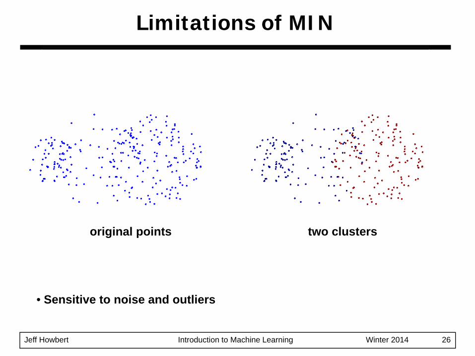
Limitations of MIN
• Sensitive to noise and outliers
original points two clusters

Jeff Howbert Introduction to Machine Learning Winter 2014 27
Similarity of two clusters is based on the two least similar (most distant) points in the different clusters– Determined by one pair of points, i.e., by one
link in the proximity graph.
Cluster similarity: MAX or complete link
I1 I2 I3 I4 I5I1 1.00 0.90 0.10 0.65 0.20I2 0.90 1.00 0.70 0.60 0.50I3 0.10 0.70 1.00 0.40 0.30I4 0.65 0.60 0.40 1.00 0.80I5 0.20 0.50 0.30 0.80 1.00 1 2 3 4 5

Jeff Howbert Introduction to Machine Learning Winter 2014 28
Hierarchical clustering: MAX
nested clusters dendrogram
3 6 4 1 2 50
0.05
0.1
0.15
0.2
0.25
0.3
0.35
0.4
1
2
3
4
5
61
2 5
3
4

Jeff Howbert Introduction to Machine Learning Winter 2014 29
Strength of MAX
• Less susceptible to noise and outliers
original points two clusters

Jeff Howbert Introduction to Machine Learning Winter 2014 30
Limitations of MAX
• Tends to break large clusters
• Biased towards globular clusters
original points two clusters

Jeff Howbert Introduction to Machine Learning Winter 2014 31
Proximity of two clusters is the average of pairwise proximity between points in the two clusters.
Need to use average connectivity for scalability since total proximity favors large clusters
Cluster similarity: group average
||Cluster||Cluster
)p,pproximity(
)Cluster,Clusterproximity(ji
ClusterpClusterp
ji
jijjii
∗=
∑∈∈
I1 I2 I3 I4 I5I1 1.00 0.90 0.10 0.65 0.20I2 0.90 1.00 0.70 0.60 0.50I3 0.10 0.70 1.00 0.40 0.30I4 0.65 0.60 0.40 1.00 0.80I5 0.20 0.50 0.30 0.80 1.00 1 2 3 4 5

Jeff Howbert Introduction to Machine Learning Winter 2014 32
Hierarchical clustering: group average
nested clusters dendrogram
3 6 4 1 2 50
0.05
0.1
0.15
0.2
0.25
1
2
3
4
5
61
2
5
3
4
Jeff Howbert Introduction to Machine Learning Winter 2014 33
Compromise between single and complete link
Strengths:– Less susceptible to noise and outliers
Limitations:– Biased towards globular clusters
Hierarchical clustering: group average

Jeff Howbert Introduction to Machine Learning Winter 2014 34
Similarity of two clusters is based on the increase in squared error when two clusters are merged– Similar to group average if distance between
points is distance squared
Less susceptible to noise and outliers
Biased towards globular clusters
Hierarchical analogue of k-means– Can be used to initialize k-means
Cluster similarity: Ward’s method

Jeff Howbert Introduction to Machine Learning Winter 2014 35
Hierarchical clustering comparison
group average
Ward’s method1
23
4
5
61
2
5
3
4
MIN MAX
1
23
4
5
61
2
5
34
1
23
4
5
61
2 5
3
41
23
4
5
61
2
3
4
5

Jeff Howbert Introduction to Machine Learning Winter 2014 36
Time and space complexity– n = number of datapoints or objects– Space requirement ~ O( n2 ) since it uses the
proximity matrix.– Time complexity ~ O( n3 ) many cases.
There are n steps and at each step the proximity matrix (size n2) must be searched and updated.
Can be reduced to O( n2 log( n ) ) time for some approaches.
Hierarchical clustering

Jeff Howbert Introduction to Machine Learning Winter 2014 37
Problems and limitations– Once a decision is made to combine two clusters, it
cannot be undone.– No objective function is directly minimized.– Different schemes have problems with one or more of
the following:Sensitivity to noise and outliersDifficulty handling different sized clusters and convex shapesBreaking large clusters
– Inherently unstable toward addition or deletion of samples.
Hierarchical clustering

Jeff Howbert Introduction to Machine Learning Winter 2014 38
Cut tree at some height to get desired number of partitions k
From hierarchical to partitional clustering
3 6 4 1 2 50
0.05
0.1
0.15
0.2
0.25 k = 2
k = 4
k = 3
Jeff Howbert Introduction to Machine Learning Winter 2014 39
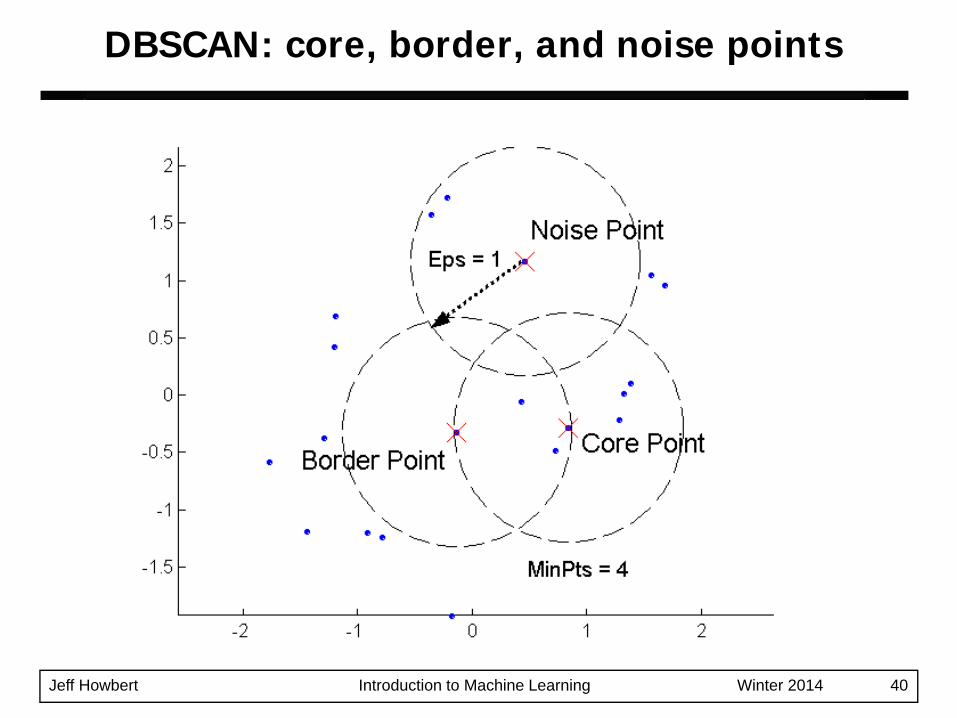
DBSCAN is a density-based algorithm.– Density = number of points within a specified
radius (Eps)– A point is a core point if it has more than a
specified number of points (MinPts) within Eps. These points are in the interior of a cluster.
– A border point has fewer than MinPts within Eps, but is in the neighborhood of a core point.
– A noise point is any point that is not a core point or a border point.
DBSCAN
Jeff Howbert Introduction to Machine Learning Winter 2014 40
DBSCAN: core, border, and noise points
Jeff Howbert Introduction to Machine Learning Winter 2014 41
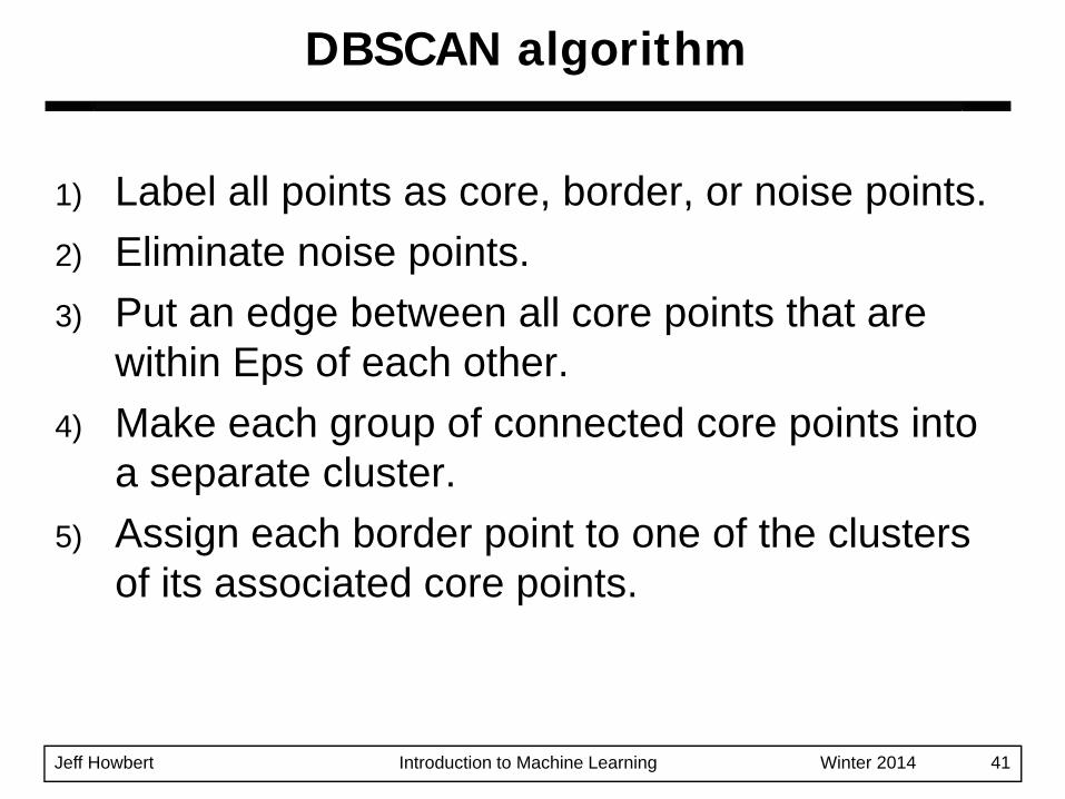
1) Label all points as core, border, or noise points.2) Eliminate noise points.3) Put an edge between all core points that are
within Eps of each other.4) Make each group of connected core points into
a separate cluster.5) Assign each border point to one of the clusters
of its associated core points.
DBSCAN algorithm
Jeff Howbert Introduction to Machine Learning Winter 2014 42
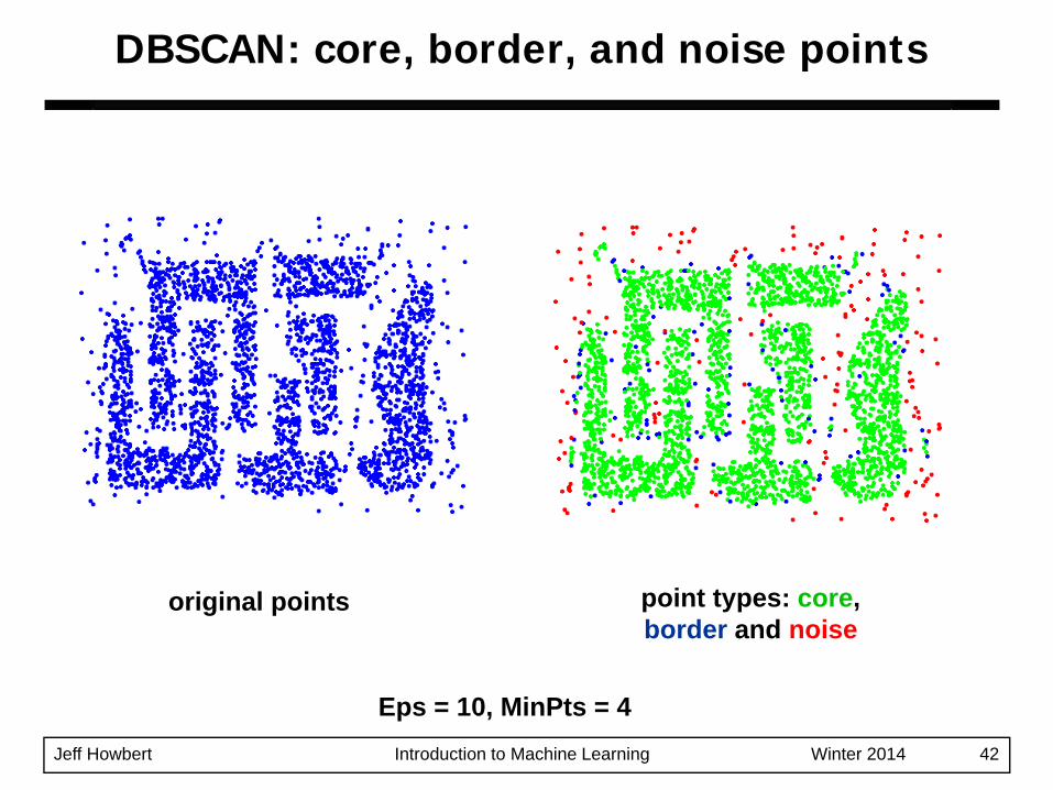
DBSCAN: core, border, and noise points
original points point types: core, border and noise
Eps = 10, MinPts = 4
Jeff Howbert Introduction to Machine Learning Winter 2014 43
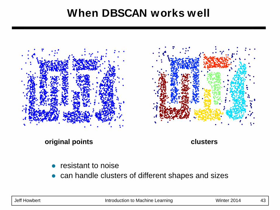
When DBSCAN works well
original points clusters
resistant to noisecan handle clusters of different shapes and sizes
Jeff Howbert Introduction to Machine Learning Winter 2014 44
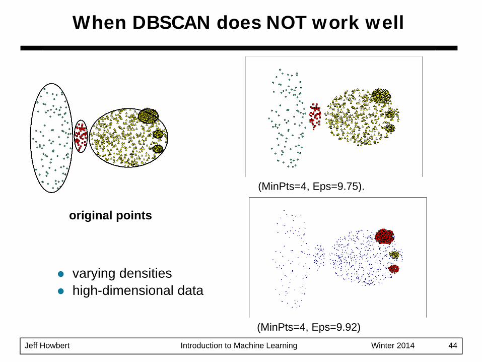
When DBSCAN does NOT work well
original points
(MinPts=4, Eps=9.75).
(MinPts=4, Eps=9.92)
varying densitieshigh-dimensional data

Jeff Howbert Introduction to Machine Learning Winter 2014 45
Idea:– for points in a cluster, their kth nearest neighbors
are at roughly the same distance– noise points have the kth nearest neighbor at
farther distance– plot sorted distance of every point to its kth
nearest neighborExample:– assume k = 4– plot sorted distances to
4th nearest neighbor– select Eps as distance
where curve has sharpelbow
DBSCAN: determining Eps and MinPts

Jeff Howbert Introduction to Machine Learning Winter 2014 46
For supervised classification we have a variety of measures to evaluate how good our model is
– Accuracy, precision, recall, squared error
For clustering, the analogous question is how to evaluate the “goodness” of the resulting clusters?
But cluster quality is often in the eye of the beholder!
It’s still important to try and measure cluster quality– To avoid finding patterns in noise– To compare clustering algorithms– To compare two sets of clusters– To compare two clusters
Cluster validity
Jeff Howbert Introduction to Machine Learning Winter 2014 47
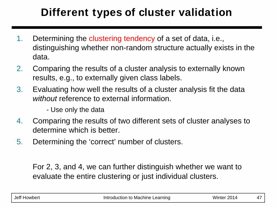
1. Determining the clustering tendency of a set of data, i.e., distinguishing whether non-random structure actually exists in the data.
2. Comparing the results of a cluster analysis to externally known results, e.g., to externally given class labels.
3. Evaluating how well the results of a cluster analysis fit the data without reference to external information.
- Use only the data4. Comparing the results of two different sets of cluster analyses to
determine which is better.5. Determining the ‘correct’ number of clusters.
For 2, 3, and 4, we can further distinguish whether we want to evaluate the entire clustering or just individual clusters.
Different types of cluster validation

Jeff Howbert Introduction to Machine Learning Winter 2014 48
Numerical measures used to judge various aspects of cluster validity are classified into the following three types:– External index: Measures extent to which cluster labels match
externally supplied class labels.Entropy
– Internal index: Measures the “goodness” of a clustering structure without respect to external information.
CorrelationVisualize similarity matrixSum of Squared Error (SSE)
– Relative index: Compares two different clusterings or clusters. Often an external or internal index is used for this function, e.g., SSE or entropy.
Measures of cluster validity

Jeff Howbert Introduction to Machine Learning Winter 2014 49
Two matrices – Proximity matrix– “Incidence” matrix
One row and one column for each data point.An entry is 1 if the associated pair of points belong to same cluster.An entry is 0 if the associated pair of points belongs to different clusters.
Compute the correlation between the two matrices– Since the matrices are symmetric, only the correlation between
n ⋅ ( n - 1 ) / 2 entries needs to be calculated.
High correlation indicates that points that belong to the same cluster are close to each other. Not a good measure for some density or contiguity based clusters.
Measuring cluster validity via correlation
Jeff Howbert Introduction to Machine Learning Winter 2014 50
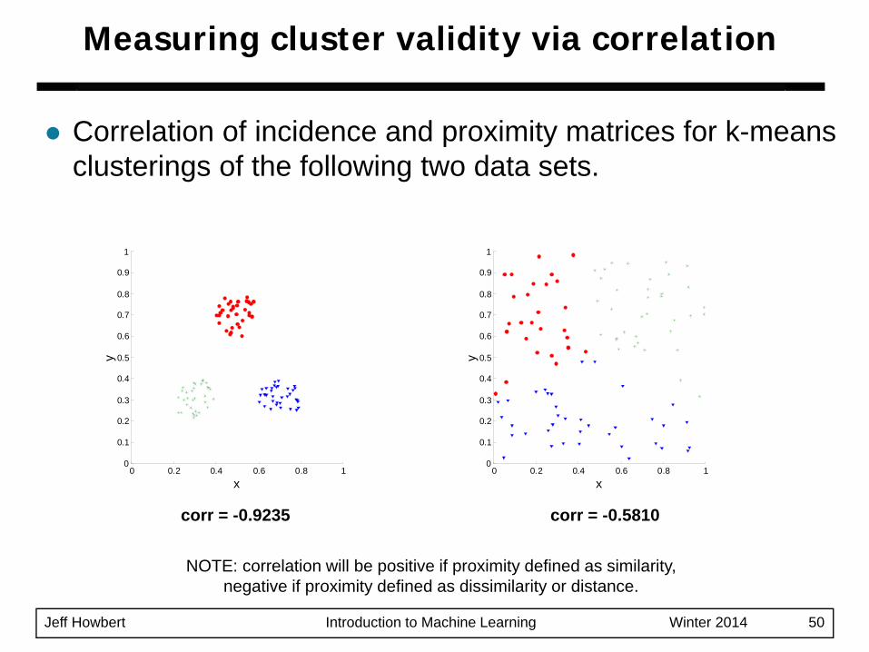
Correlation of incidence and proximity matrices for k-means clusterings of the following two data sets.
Measuring cluster validity via correlation
0 0.2 0.4 0.6 0.8 10
0.1
0.2
0.3
0.4
0.5
0.6
0.7
0.8
0.9
1
x
y
0 0.2 0.4 0.6 0.8 10
0.1
0.2
0.3
0.4
0.5
0.6
0.7
0.8
0.9
1
xy
corr = -0.9235 corr = -0.5810
NOTE: correlation will be positive if proximity defined as similarity, negative if proximity defined as dissimilarity or distance.
Jeff Howbert Introduction to Machine Learning Winter 2014 51
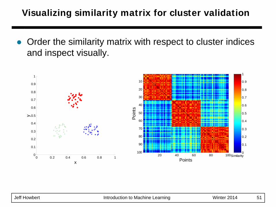
Order the similarity matrix with respect to cluster indices and inspect visually.
Visualizing similarity matrix for cluster validation
0 0.2 0.4 0.6 0.8 10
0.1
0.2
0.3
0.4
0.5
0.6
0.7
0.8
0.9
1
x
y
Points
Poin
ts
20 40 60 80 100
10
20
30
40
50
60
70
80
90
100Similarity
0
0.1
0.2
0.3
0.4
0.5
0.6
0.7
0.8
0.9
1
Jeff Howbert Introduction to Machine Learning Winter 2014 52
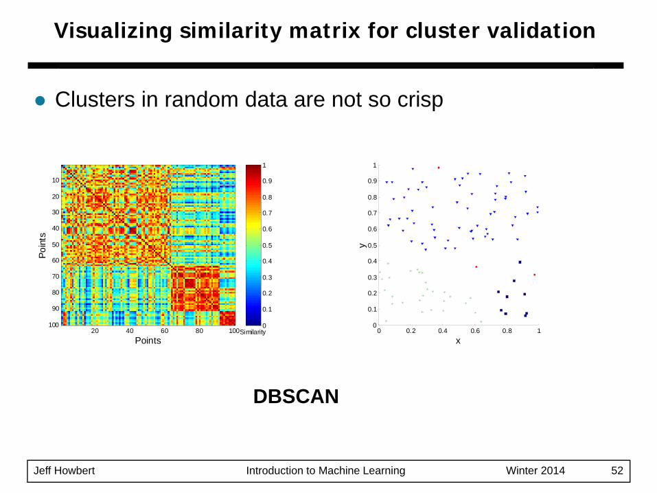
Clusters in random data are not so crisp
Visualizing similarity matrix for cluster validation
Points
Poin
ts
20 40 60 80 100
10
20
30
40
50
60
70
80
90
100Similarity
0
0.1
0.2
0.3
0.4
0.5
0.6
0.7
0.8
0.9
1
DBSCAN
0 0.2 0.4 0.6 0.8 10
0.1
0.2
0.3
0.4
0.5
0.6
0.7
0.8
0.9
1
x
y

Jeff Howbert Introduction to Machine Learning Winter 2014 53
Points
Poin
ts
20 40 60 80 100
10
20
30
40
50
60
70
80
90
100Similarity
0
0.1
0.2
0.3
0.4
0.5
0.6
0.7
0.8
0.9
1
Clusters in random data are not so crisp
Visualizing similarity matrix for cluster validation
k-means
0 0.2 0.4 0.6 0.8 10
0.1
0.2
0.3
0.4
0.5
0.6
0.7
0.8
0.9
1
x
y
Jeff Howbert Introduction to Machine Learning Winter 2014 54
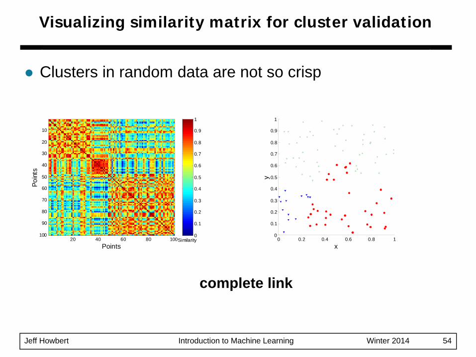
Clusters in random data are not so crisp
Visualizing similarity matrix for cluster validation
0 0.2 0.4 0.6 0.8 10
0.1
0.2
0.3
0.4
0.5
0.6
0.7
0.8
0.9
1
x
y
Points
Poin
ts
20 40 60 80 100
10
20
30
40
50
60
70
80
90
100Similarity
0
0.1
0.2
0.3
0.4
0.5
0.6
0.7
0.8
0.9
1
complete link

Jeff Howbert Introduction to Machine Learning Winter 2014 55
Visualizing similarity matrix for cluster validation
1 2
3
5
6
4
7
DBSCAN
0
0.1
0.2
0.3
0.4
0.5
0.6
0.7
0.8
0.9
1
500 1000 1500 2000 2500 3000
500
1000
1500
2000
2500
3000
Not as useful when clusters are non-globular
Jeff Howbert Introduction to Machine Learning Winter 2014 56
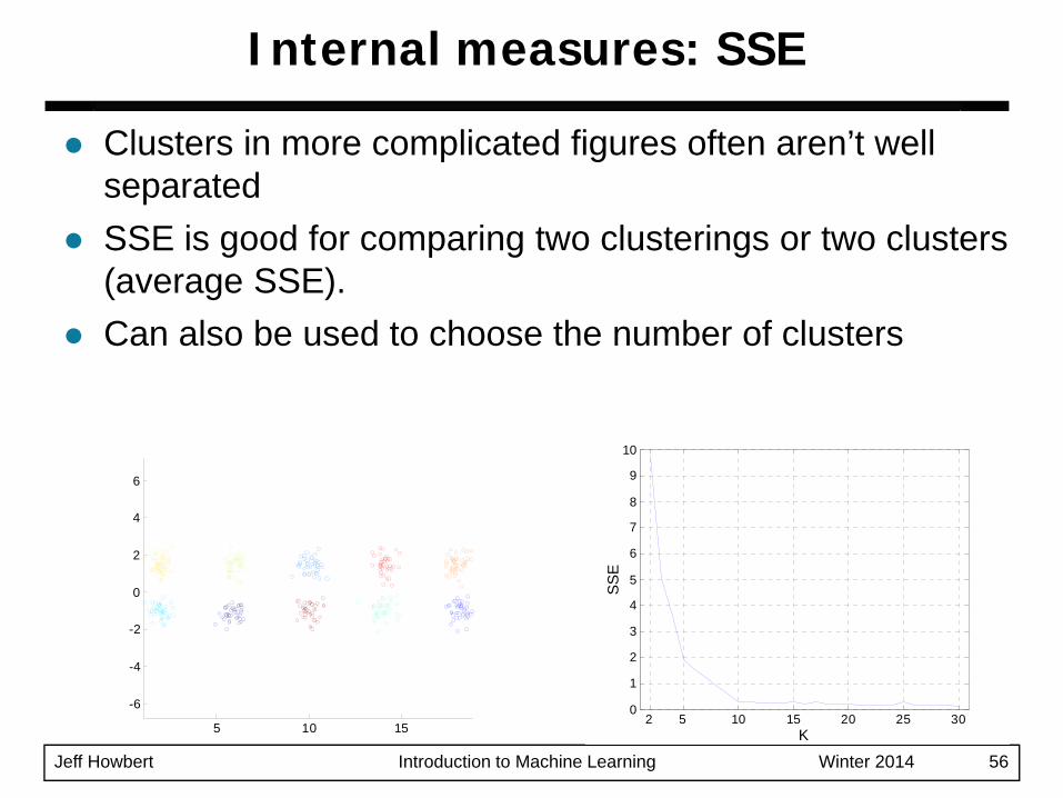
Clusters in more complicated figures often aren’t well separatedSSE is good for comparing two clusterings or two clusters (average SSE).Can also be used to choose the number of clusters
Internal measures: SSE
2 5 10 15 20 25 300
1
2
3
4
5
6
7
8
9
10
K
SSE
5 10 15
-6
-4
-2
0
2
4
6
Jeff Howbert Introduction to Machine Learning Winter 2014 57
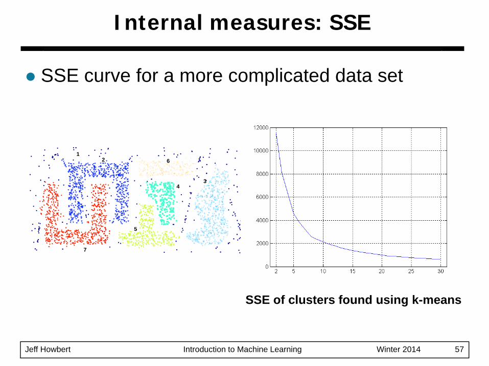
SSE curve for a more complicated data set
Internal measures: SSE
1 2
3
5
6
4
7
SSE of clusters found using k-means

Jeff Howbert Introduction to Machine Learning Winter 2014 58
Need a framework to interpret any measure. – For example, if our measure of evaluation has the value 10, is that
good, fair, or poor?
Statistics provide a framework for cluster validity– The more “atypical” a clustering result is, the more likely it represents
valid structure in the data– Can compare the values of an index that result from random data or
clusterings to those of a clustering result.If the value of the index is unlikely, then the cluster results are valid
– These approaches are more complicated and harder to understand.
For comparing the results of two different sets of cluster analyses, a framework is less necessary.
– However, there is the question of whether the difference between two index values is significant
Framework for cluster validity

Jeff Howbert Introduction to Machine Learning Winter 2014 59
Example– Compare SSE of 0.005 for three true clusters against SSEs for
three clusters in random data– Histogram shows distributions of SSEs for 500 sets of three
clusters in random data points (100 data points randomly placed in range 0.2 - 0.8 for x and y)
Statistical framework for SSE
0.016 0.018 0.02 0.022 0.024 0.026 0.028 0.03 0.032 0.0340
5
10
15
20
25
30
35
40
45
50
SSE
Cou
nt
0 0.2 0.4 0.6 0.8 10
0.1
0.2
0.3
0.4
0.5
0.6
0.7
0.8
0.9
1
x
y

Jeff Howbert Introduction to Machine Learning Winter 2014 60
Correlation of incidence and proximity matrices for the k-means clusterings of the following two data sets.
Statistical framework for correlation
0 0.2 0.4 0.6 0.8 10
0.1
0.2
0.3
0.4
0.5
0.6
0.7
0.8
0.9
1
x
y
0 0.2 0.4 0.6 0.8 10
0.1
0.2
0.3
0.4
0.5
0.6
0.7
0.8
0.9
1
x
y
corr = -0.9235 corr = -0.5810

Jeff Howbert Introduction to Machine Learning Winter 2014 61
“The validation of clustering structures is the most difficult and frustrating part of cluster analysis.
Without a strong effort in this direction, cluster analysis will remain a black art accessible only to those true believers who have experience and great courage.”
Algorithms for Clustering Data, Jain and Dubes, 1988
Final comment on cluster validity

Jeff Howbert Introduction to Machine Learning Winter 2014 62
MATLAB interlude
matlab_demo_12.m