clustering: introduction adriano joaquim de o cruz ©2002 nce/ufrj [email protected]

Clustering: Introduction

Adriano Joaquim de O Cruz ©2002

NCE/UFRJ

[email protected]

IntroductionIntroduction

*@2001 Adriano Cruz *NCE e IM - UFRJ Cluster 3

What is cluster analysis?What is cluster analysis?

The process of grouping a set of The process of grouping a set of physical or abstract objects into classes physical or abstract objects into classes of similar objects.of similar objects.

The class label of each class is The class label of each class is unknown.unknown.

Classification separates objects into Classification separates objects into classes when the labels are known.classes when the labels are known.


What is cluster analysis? What is cluster analysis? cont.cont.

Clustering is a form of learning by Clustering is a form of learning by observations.observations.

Neural Networks learn by examples.Neural Networks learn by examples. Unsupervised learning.Unsupervised learning.


ApplicationsApplications

In business helps to discover distinct In business helps to discover distinct groups of customers.groups of customers.

In data mining used to gain insight into In data mining used to gain insight into the distribution of data, to observe the the distribution of data, to observe the characteristics of each cluster.characteristics of each cluster.

Pre-processing step for classification.Pre-processing step for classification. Pattern recognition.Pattern recognition.


RequirementsRequirements

Scalability: work with large databases.Scalability: work with large databases.

Ability to deal with different types of Ability to deal with different types of attributes (not only interval based data).attributes (not only interval based data).

Clusters of arbitrary shape, not only Clusters of arbitrary shape, not only spherical.spherical.

Minimal requirements about domain.Minimal requirements about domain.

Ability do deal with noisy data.Ability do deal with noisy data.


Requirements Requirements cont.cont.

Insensitivity to the order of input records.Insensitivity to the order of input records.

Work with samples of high Work with samples of high dimensionality.dimensionality.

Constrained-based clusteringConstrained-based clustering

Interpretability and usability: results Interpretability and usability: results should be easily interpretable.should be easily interpretable.


Sensitivity to Input OrderSensitivity to Input Order

Some algorithms are sensitive to the Some algorithms are sensitive to the order of input dataorder of input data

Leader algorithm is an exampleLeader algorithm is an example Ellipse: 2 1 3 5 4 6; Triangle: 1 2 6 4 5 3 Ellipse: 2 1 3 5 4 6; Triangle: 1 2 6 4 5 3

Clustering TechniquesClustering Techniques


Heuristic Clustering TechniquesHeuristic Clustering Techniques

Incomplete or heuristic clustering: geometrical Incomplete or heuristic clustering: geometrical methods or projection techniques.methods or projection techniques.

Dimension reduction techniques (e.g. PCA) are Dimension reduction techniques (e.g. PCA) are used obtain a graphical representation in two or used obtain a graphical representation in two or three dimensions.three dimensions.

Heuristic methods based on visualisation are Heuristic methods based on visualisation are used to determine the clusters.used to determine the clusters.


Deterministic Crisp ClusteringDeterministic Crisp Clustering

Each datum will be assigned to only one Each datum will be assigned to only one cluster.cluster.

Each cluster partition defines a ordinary Each cluster partition defines a ordinary partition of the data set.partition of the data set.


Overlapping Crisp ClusteringOverlapping Crisp Clustering

Each datum will be assigned to at least Each datum will be assigned to at least one cluster.one cluster.

Elements may belong to more than one Elements may belong to more than one cluster at various degrees.cluster at various degrees.


Probabilistic ClusteringProbabilistic Clustering

For each element, a probabilistic distribution For each element, a probabilistic distribution over the clusters is determined.over the clusters is determined.

The distribution specifies the probability with The distribution specifies the probability with which a datum is assigned to a cluster.which a datum is assigned to a cluster.

If the probabilities are interpreted as degree If the probabilities are interpreted as degree of membership then these are fuzzy of membership then these are fuzzy clustering techniques.clustering techniques.


Possibilistic ClusteringPossibilistic Clustering

Degrees of membership or possibility Degrees of membership or possibility indicate to what extent a datum belongs indicate to what extent a datum belongs to the clusters.to the clusters.

Possibilistic cluster analysis drops the Possibilistic cluster analysis drops the constraint that the sum of memberships constraint that the sum of memberships of each datum to all clusters is equal to of each datum to all clusters is equal to one.one.


Hierarchical ClusteringHierarchical Clustering

Descending techniques: they divide the Descending techniques: they divide the data into more fine-grained classes.data into more fine-grained classes.

Ascending techniques: they combine Ascending techniques: they combine small classes into more coarse-grained small classes into more coarse-grained ones.ones.


Objective Function ClusteringObjective Function Clustering

An objective function assigns to An objective function assigns to each cluster partition values that each cluster partition values that have to be optimised.have to be optimised.

This is strictly an optimisation This is strictly an optimisation problem.problem.

Data TypesData Types


Data Types Data Types

Interval-scaledInterval-scaled variables are continuous variables are continuous measurements of a linear scale. Ex. measurements of a linear scale. Ex. height, weight, temperature.height, weight, temperature.

Binary variablesBinary variables have only two states. have only two states. Ex. smoker, fever, client, owner.Ex. smoker, fever, client, owner.

Nominal variablesNominal variables are a generalisation are a generalisation of a binary variable with m states. Ex. of a binary variable with m states. Ex. Map colour, Marital state.Map colour, Marital state.


Data Types Data Types cont.cont.

Ordinal variablesOrdinal variables are ordered nominal are ordered nominal variables. Ex. Olympic medals, variables. Ex. Olympic medals, Professional ranks.Professional ranks.

Ratio-scaledRatio-scaled variables have a non- variables have a non-linear scale. Ex. Growth of a bacteria linear scale. Ex. Growth of a bacteria population population


Interval-scaled variables Interval-scaled variables

Interval-scaledInterval-scaled variables are continuous variables are continuous measurements of a linear scale. Ex. measurements of a linear scale. Ex. height, weight, temperature.height, weight, temperature.

Interval-scaled variables are dependent Interval-scaled variables are dependent on the units used.on the units used.

Measurement unit can affect analysis, Measurement unit can affect analysis, so standardisation should be used.so standardisation should be used.


ProblemsProblems

Person Age (yr) Height (cm)

A 35 190

B 40 190

C 35 160

D 40 160


StandardisationStandardisation

Converting original measurements to Converting original measurements to unitless values.unitless values.

Attempts to give all variables the equal Attempts to give all variables the equal weight.weight.

Useful when there is no prior knowledge Useful when there is no prior knowledge of the data.of the data.


Standardisation algorithmStandardisation algorithm

Z-scores indicate how far and in what direction Z-scores indicate how far and in what direction an item deviates from its distribution's mean, an item deviates from its distribution's mean, expressed in units of its distribution's standard expressed in units of its distribution's standard deviation.deviation.

The transformed scores will have a mean of zero The transformed scores will have a mean of zero and standard deviation of one.and standard deviation of one.

It is useful when comparing relative standings of It is useful when comparing relative standings of items from distributions with different means items from distributions with different means and/or different standard deviation.and/or different standard deviation.


Standardisation algorithmStandardisation algorithm

Consider Consider nn values of a variable values of a variable xx..

Calculate the mean value.Calculate the mean value.

Calculate the standard deviation.Calculate the standard deviation.

Calculate the z-score. Calculate the z-score.

n

iixn

x1

1

n

xxn

ii

x

1

2)(

x

ix

xxz

i


Z-scores exampleZ-scores example

Sample Heights Ages z-heights z-ages1 137,16 10 -0,45 -0,612 195,58 25 1,58 0,393 170,18 55 0,7 2,394 172,73 32 0,79 0,865 116,84 8 -1,16 -0,746 162,56 11 0,43 -0,547 157,48 9 0,26 -0,678 142,24 15 -0,28 -0,279 96,52 7 -1,87 -0,81

Means 150,14 19,11 0 028,67 15,01 1 1Std Dev


Real heights and ages chartsReal heights and ages charts

Row 2

Row 3

Row 4

Row 5

Row 6

Row 7

Row 8

Row 9

Row 10

0

25

50

75

100

125

150

175

200

Real Heights and Ages

Heights

Ages

Samples

He

ights

and

Ag

es


Z-scores for heights and agesZ-scores for heights and ages

Row 2

Row 3

Row 4

Row 5

Row 6

Row 7

Row 8

Row 9

Row 10

-2

-1,5

-1

-0,5

0

0,5

1

1,5

2

2,5

Z-scores for heights and ages

Z-heights

Z-ages

Samples

Heig

hts

and a

ges


Data chartData chart

Real data

0

20

40

60

0,00 50,00 100,00 150,00 200,00 250,00

Heights

Age

s

Ages


Data chartData chart

Z-score data

-1,00

0,00

1,00

2,00

3,00

-3,00 -1,00 1,00

heights

Ag

es

Seqüência1

SimilaritiesSimilarities


Data MatricesData Matrices

Data matrix: represents Data matrix: represents nn objects with objects with pp characteristics. characteristics. Ex. Ex. personperson = { = {age, sex, incomeage, sex, income, ...}, ...}

Dissimilarity matrix: represents a Dissimilarity matrix: represents a collection of dissimilarities between all collection of dissimilarities between all pairs of objects.pairs of objects.


DissimilaritiesDissimilarities

Dissimilarity measures some form of Dissimilarity measures some form of distance between objects.distance between objects.

Clustering algorithms use dissimilarities Clustering algorithms use dissimilarities to cluster data.to cluster data.

How can dissimilarities be measured? How can dissimilarities be measured?


How to calculate dissimilarities?How to calculate dissimilarities?

The most popular methods are based on the The most popular methods are based on the distance between pairs of objects.distance between pairs of objects.

Minkowski distance:Minkowski distance:

pp is the number of characteristics is the number of characteristics qq is the distance type is the distance type qq=2 (Euclides distance), =2 (Euclides distance), qq=1 (Manhattan)=1 (Manhattan)

p

j

qq

kjijki xxd1

1

)(),( xx


SimilaritiesSimilarities

It is also possible to work with It is also possible to work with similarities [similarities [ss((xxii,,xxjj)])]

0<=0<=ss((xxii,,xxjj)<=1)<=1

ss((xxii,,xxii)=1)=1

ss((xxii,,xxjj)=)=ss((xxjj,,xxii))

It is possible to consider that It is possible to consider that dd((xxii,,xxjj)=1-)=1-

ss((xxii,,xxjj))


DistancesDistances

Sample Heights Ages Z-heights Z-ages Euclides Manhatann Euclides Manhatann1 137,16 10 -0,45 -0,61 15,8613 22,0944 0,7574 1,05992 195,58 25 1,58 0,39 45,8167 51,3256 1,6325 1,97703 170,18 55 0,70 2,39 41,1033 55,9256 2,4915 3,09034 172,73 32 0,79 0,86 26,0054 35,4756 1,1654 1,64665 116,84 8 -1,16 -0,74 35,1080 44,4144 1,3774 1,90186 162,56 11 0,43 -0,54 14,8312 20,5278 0,6926 0,97357 157,48 9 0,26 -0,67 12,4924 17,4478 0,7207 0,92968 142,24 15 -0,28 -0,27 8,9086 12,0144 0,3886 0,54969 96,52 7 -1,87 -0,81 54,9740 65,7344 2,0368 2,6771

Means 150,14 19,11 0,0000 0,0000 2 1 2 1Std Dev 28,67 15,01 1,0000 1,0000


DissimilaritiesDissimilarities

There are other ways to obtain There are other ways to obtain dissimilarities.dissimilarities.

So we no longer speak of distances.So we no longer speak of distances. Basically dissimilarities are nonnegative Basically dissimilarities are nonnegative

numbers (numbers (dd((ii,,jj)) that are small (close to )) that are small (close to 0) when 0) when ii and and jj are similar. are similar.


PearsonPearson

Pearson product-moment correlation Pearson product-moment correlation between variables f and gbetween variables f and g

Coefficients lie between –1 and +1Coefficients lie between –1 and +1

n

ifig

n

ifif

n

igigfif

mxmx

mxmxgfR

1

2

1

2

1

)()(

))((),(


Pearson - Pearson - contcont

A correlation of +1 means that there is a A correlation of +1 means that there is a perfect positive linear relationship perfect positive linear relationship between variables. between variables.

A correlation of -1 means that there is a A correlation of -1 means that there is a perfect negative linear relationship perfect negative linear relationship between variables. between variables.

A correlation of 0 means there is no A correlation of 0 means there is no linear relationship between the two linear relationship between the two variables. variables.


Pearson - exPearson - ex

ryz = 0.9861ryz = 0.9861; ; ryw = -0.9551ryw = -0.9551; ; ryr=ryr= 0.27700.2770


Correlation and dissimilarities 1Correlation and dissimilarities 1

dd((f,gf,g)=(1-)=(1-R(f,gR(f,g))/2 (1)))/2 (1)

Variables with a high positive correlation Variables with a high positive correlation (+1) receive a dissimilarity close to 0(+1) receive a dissimilarity close to 0

Variables with strongly negative Variables with strongly negative correlation will be considered very correlation will be considered very dissimilardissimilar


Correlation and dissimilarities 2Correlation and dissimilarities 2

dd((f,gf,g)=1-|)=1-|R(f,gR(f,g)| (2))| (2)

Variables with a high positive correlation Variables with a high positive correlation (+1) and negative correlation will (+1) and negative correlation will receive a dissimilarity close to 0receive a dissimilarity close to 0


Numerical ExampleNumerical Example

Name Weight Height Month Year

Ilan 15 95 1 82

Jack 49 156 5 55

Kim 13 95 11 81

Lieve 45 160 7 56

Leon 85 178 6 48

Peter 66 176 6 56

Talia 12 90 12 83

Tina 10 78 1 84


Numerical Example 1Numerical Example 1

Quanti Weight Height Month Year

Corr Weight 1

Height 0.957 1

Month -0.036 0.021 1

Year -0.953 -0.985 0.013 1

Diss Weight 0

(1) Height 0.021 0

Month 0.518 0.489 0

Year 0.977 0.992 0.493 0

Diss Weight 0

(2) Height 0.043 0

Month 0.964 0.979 0

Year 0.047 0.015 0.987 0


Binary VariablesBinary Variables

Binary variables have only two states.Binary variables have only two states. States can be symmetric or asymmetric.States can be symmetric or asymmetric. Binary variables are symmetric if both Binary variables are symmetric if both

states are equally valuable. Ex. genderstates are equally valuable. Ex. gender When the states are not equally When the states are not equally

important the variable is asymmetric. important the variable is asymmetric. Ex. disease tests (1-positive; 0-negative) Ex. disease tests (1-positive; 0-negative)


Contingency tablesContingency tables

Consider objects described by Consider objects described by pp binary binary variablesvariables

qq variables are equal to one on variables are equal to one on ii and and jj rr variables are 1 on variables are 1 on ii and 0 on object and 0 on object jj

Object j 1 0 Sum

1 q r q+r 0 s t s+t

Object i

Sum q+s r+t p


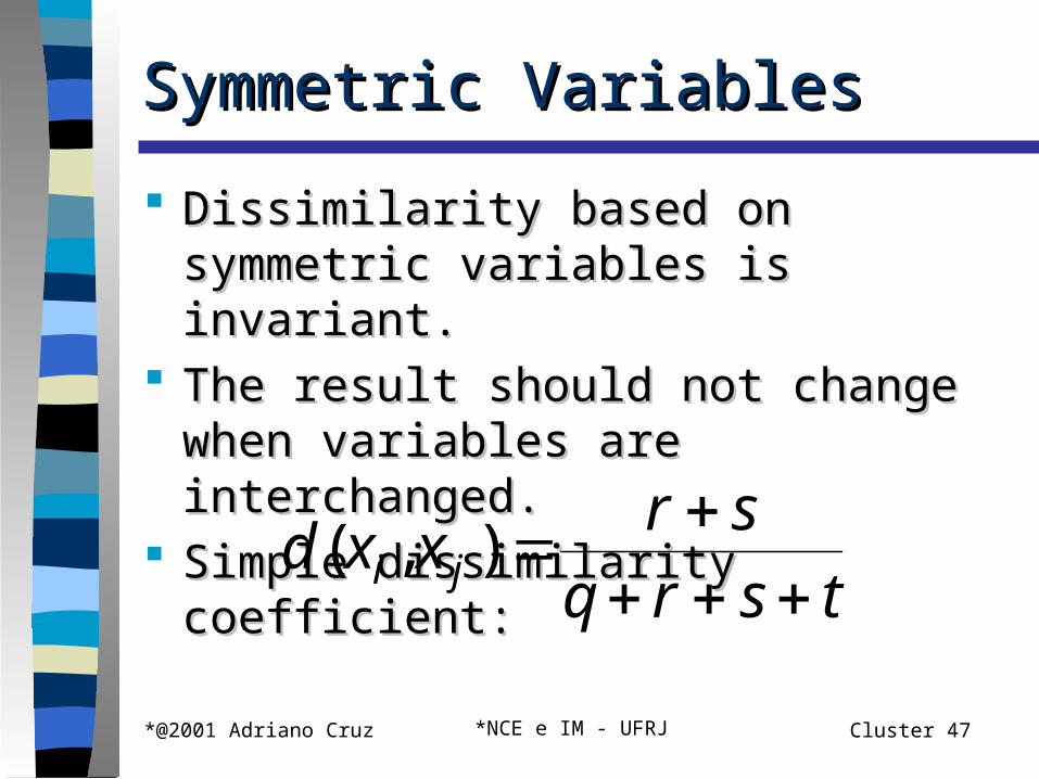
Symmetric VariablesSymmetric Variables

Dissimilarity based on symmetric Dissimilarity based on symmetric variables is invariant. variables is invariant.

The result should not change when The result should not change when variables are interchanged.variables are interchanged.

Simple dissimilarity coefficient:Simple dissimilarity coefficient:

tsrq

srxxd ji

),(


Symmetric VariablesSymmetric Variables

DissimilarityDissimilarity

SimilaritySimilarity

tsrq

srxxd ji

),(

tsrqtq

xxs ji ),(


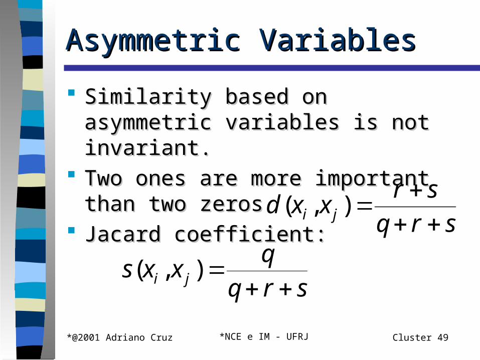
Asymmetric VariablesAsymmetric Variables

Similarity based on asymmetric Similarity based on asymmetric variables is not invariant.variables is not invariant.

Two ones are more important than two Two ones are more important than two zeroszeros

Jacard coefficient:Jacard coefficient:srqsr

xxd ji

),(

srqq

xxs ji ),(


Computing dissimilaritiesComputing dissimilarities

Name fever cough Test1 Test2 Test3 Test4

Jack Y N P N N N

Mary Y N P N P N

Jim Y Y N N N N


Computing DissimilaritiesComputing Dissimilarities

Jack Mary q 1,1 r 1,0 s 0,1 t 0,0

Fever Y Y 1 0 0 0

Cough N N 0 0 0 1

Test1 P P 1 0 0 0

Test2 N N 0 0 0 1

Test3 N P 0 0 1 0

Test4 N N 0 0 0 1

2 0 1 3



75.0211

21),(

67.0111

11),(

33.0102

10),(

maryjimd

jimjackd

srqsr

maryjackd

•Jim and Mary have the highest dissimilarity value, so they have low probability of having the same disease.


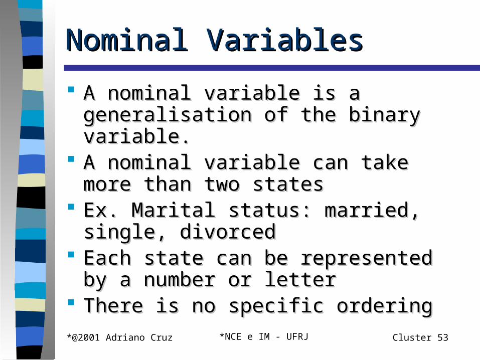
Nominal VariablesNominal Variables

A nominal variable is a generalisation of A nominal variable is a generalisation of the binary variable.the binary variable.

A nominal variable can take more than A nominal variable can take more than two statestwo states

Ex. Marital status: married, single, Ex. Marital status: married, single, divorceddivorced

Each state can be represented by a Each state can be represented by a number or letternumber or letter

There is no specific orderingThere is no specific ordering



Consider two objects Consider two objects ii and and jj, described , described by nominal variablesby nominal variables

Each object has Each object has pp characteristics characteristics

mm is the number of matches is the number of matches

pmp

jid

),(


Binarising nominal variablesBinarising nominal variables

An nominal variable can encoded to create a An nominal variable can encoded to create a new binary variable for each statenew binary variable for each state

Example:Example: Marital state = {married, single, divorced}Marital state = {married, single, divorced} Married: 1=yes – 0=noMarried: 1=yes – 0=no Single: 1=yes – 0=noSingle: 1=yes – 0=no Divorced: 1=yes – 0=noDivorced: 1=yes – 0=no Ex. Marital state = {married}Ex. Marital state = {married} married = 1, single = 0, divorced = 0 married = 1, single = 0, divorced = 0


Ordinal variablesOrdinal variables

A discrete ordinal variable is similar to a A discrete ordinal variable is similar to a nominal variable, except that the states nominal variable, except that the states are ordered in a meaningful sequenceare ordered in a meaningful sequence

Ex. Bronze, silver and gold medalsEx. Bronze, silver and gold medals Ex. Assistant, associate, full memberEx. Assistant, associate, full member



Consider Consider nn objects defined by a set of objects defined by a set of ordinal variables ordinal variables

ff is one of these ordinal variables and is one of these ordinal variables and have have MMff states. states.

These states define the ranking These states define the ranking rrff {1,…, {1,…, MMff}.}.


Steps to calculate dissimilaritiesSteps to calculate dissimilarities

Assume that the value of Assume that the value of ff for the for the ithith object is object is xxifif. . Replace each Replace each xxifif by its corresponding rank by its corresponding rank rrifif {1, {1,…,…,MMff}}..

Since the number of states of each variable Since the number of states of each variable differs, it is often necessary map the range onto differs, it is often necessary map the range onto [0.0,1.0] using the equation[0.0,1.0] using the equation

Dissimilarity can be computed using distance Dissimilarity can be computed using distance measures of interval-scaled variablesmeasures of interval-scaled variables

1

1

f

ifif M

rz


Ratio-scaled variablesRatio-scaled variables

Variables on a non-linear scale, such as Variables on a non-linear scale, such as exponentialexponential

To compute dissimilarities there are To compute dissimilarities there are three methodsthree methods• Treat as interval-scaled. Not always good.Treat as interval-scaled. Not always good.• Apply a transformation like Apply a transformation like y=log(x)y=log(x) and and

treat as interval-scaledtreat as interval-scaled• Treat as ordinal data and assume ranks as Treat as ordinal data and assume ranks as

interval-scaledinterval-scaled


Variables of mixed typesVariables of mixed types

One technique is to bring all variables onto a One technique is to bring all variables onto a common scale of the interval [0.0.1.0]common scale of the interval [0.0.1.0]

Suppose that the data set contains Suppose that the data set contains pp variables of mixed type. Dissimilarity is variables of mixed type. Dissimilarity is between between ii and and jj is is

p

f

fij

p

f

fij

fij d

jid

1

)(

1

)()(

),(


Dissimilarity is between Dissimilarity is between ii and and jj is is

Variables of mixed typesVariables of mixed types

otherwise

cassymmetriisfandxxif

existnotdoesxorxif

where

d

jid

jfif

jfiff

ij

p

f

fij

p

f

fij

fij

1

00

0

),(

)(

1

)(

1

)()(


The contribution of each variable is dependent on its The contribution of each variable is dependent on its typetype

f is binary or nominal:f is binary or nominal:

f is interval-based: f is interval-based:

f is ordinal of ratio-scaled: compute ranks and treat f is ordinal of ratio-scaled: compute ranks and treat as interval-basedas interval-based

Variables of mixed types contVariables of mixed types cont

1;0)( otherwisexxifd jfiffij

)min()max()(

ff

jfiffij xx

xxd

Clustering MethodsClustering Methods


Classification typesClassification types

Clustering is an unsupervised methodClustering is an unsupervised method


Clustering MethodsClustering Methods

PartitioningPartitioning

HierarchicalHierarchical

Density-basedDensity-based

Grid-basedGrid-based

Model-basedModel-based


Partitioning MethodsPartitioning Methods

Given Given nn objects objects kk partitions are created. partitions are created.

Each partition must contain at least one Each partition must contain at least one element.element.

It uses an iterative relocation technique It uses an iterative relocation technique to improve partitioning.to improve partitioning.

Distance is the usual criterion.Distance is the usual criterion.


Partitioning Methods cont.Partitioning Methods cont.

They work well for finding spherical-shaped They work well for finding spherical-shaped clusters.clusters.

They are not efficient on very large They are not efficient on very large databases.databases.

K-means where each cluster is represented K-means where each cluster is represented by the mean value of the objects in the by the mean value of the objects in the cluster.cluster.

K-medoids where each cluster is represented K-medoids where each cluster is represented by an object near the centre of the cluster.by an object near the centre of the cluster.


Hierarchical MethodsHierarchical Methods

Creates a hierarchical decomposition of the setCreates a hierarchical decomposition of the set Agglomerative approaches start with each object Agglomerative approaches start with each object

forming a separate groupforming a separate group Merges objects or groups until all objects belong Merges objects or groups until all objects belong

to one group or a termination condition occursto one group or a termination condition occurs Divisive approaches starts with all objects in the Divisive approaches starts with all objects in the

same clustersame cluster Each successive iteration splits a cluster until all Each successive iteration splits a cluster until all

objects are on separate clusters or a termination objects are on separate clusters or a termination condition occurscondition occurs


Hierarchical Clustering contHierarchical Clustering cont

Definition of cluster proximity.Definition of cluster proximity. Min: most similar (sensitive to noise)Min: most similar (sensitive to noise) Max: most dissimilar (break large Max: most dissimilar (break large

clustersclusters


Density-based methodsDensity-based methods

Method creates clusters until the density Method creates clusters until the density in the neighbourhood exceeds some in the neighbourhood exceeds some thresholdthreshold

Able to find clusters of arbitrary shapesAble to find clusters of arbitrary shapes


Grid-based methodsGrid-based methods

Grid methods divide the object space into finite Grid methods divide the object space into finite number of cells forming a grid-like structure.number of cells forming a grid-like structure.

Cells that contain more than a certain number Cells that contain more than a certain number of elements are treated as dense.of elements are treated as dense.

Dense cells are connected to form clusters.Dense cells are connected to form clusters. Fast processing time, independent of the Fast processing time, independent of the

number of objects.number of objects. STING and CLIQUE are examples.STING and CLIQUE are examples.


Model-based methodsModel-based methods

Model-based methods hypothesise a Model-based methods hypothesise a model for each cluster and find the best model for each cluster and find the best fit of the data to the given model.fit of the data to the given model.

Statistical modelsStatistical models SOM networksSOM networks


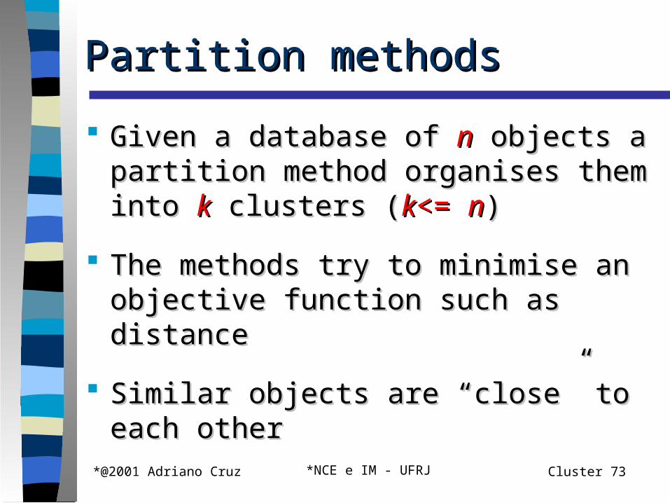
Partition methodsPartition methods

Given a database of Given a database of nn objects a partition objects a partition method organises them into method organises them into kk clusters clusters ((kk<= <= nn))

The methods try to minimise an objective The methods try to minimise an objective function such as distancefunction such as distance

Similar objects are “close” to each otherSimilar objects are “close” to each other

clustering: introduction adriano joaquim de o cruz ©2002 nce/ufrj [email protected]

Documents

nce e im ufrj cluster

adriano cruz

cluster partition

possibilistic cluster

introduction slide

probabilistic clustering

clustering interpretability

fuzzy clustering techniques