Clustering

1

Hypothesis

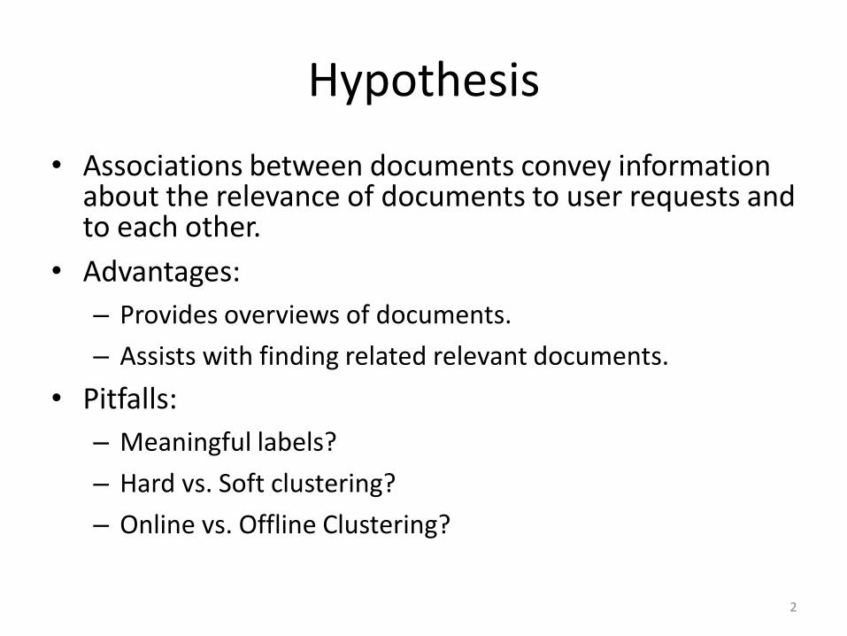
• Associations between documents convey information about the relevance of documents to user requests and to each other.

• Advantages:

– Provides overviews of documents.

– Assists with finding related relevant documents.

• Pitfalls:

– Meaningful labels?

– Hard vs. Soft clustering?

– Online vs. Offline Clustering?

2

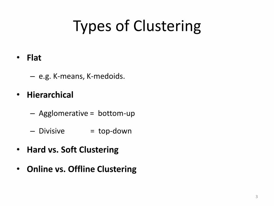
Types of Clustering

• Flat

– e.g. K-means, K-medoids.

• Hierarchical

– Agglomerative = bottom-up

– Divisive = top-down

• Hard vs. Soft Clustering

• Online vs. Offline Clustering

3

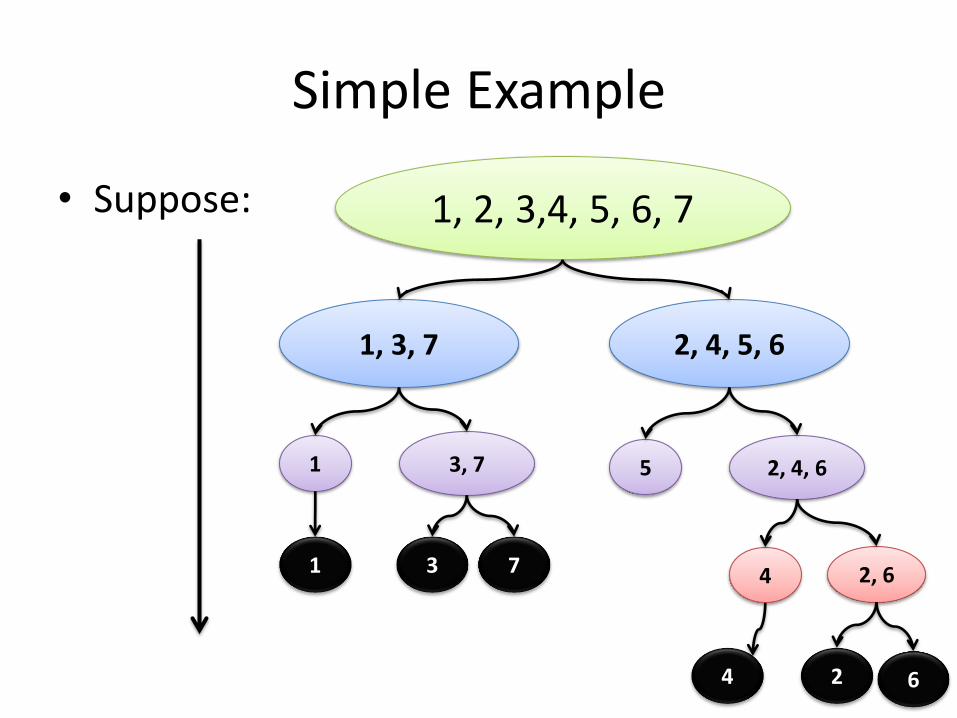
Simple Example

• Suppose: 1, 2, 3,4, 5, 6, 7

1, 3, 7 2, 4, 5, 6

1 3, 7 5 2, 4, 6

4 2, 6

4 6 2 4

7 3 1

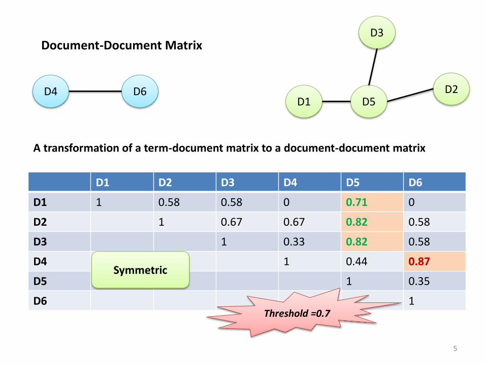
Document-Document Matrix

D1 D2 D3 D4 D5 D6

D1 1 0.58 0.58 0 0.71 0

D2 1 0.67 0.67 0.82 0.58

D3 1 0.33 0.82 0.58

D4 1 0.44 0.87

D5 1 0.35

D6 1

Symmetric

A transformation of a term-document matrix to a document-document matrix

D5 D1 D2

D3

D4 D6

5

Threshold =0.7

Clustering, cont’d

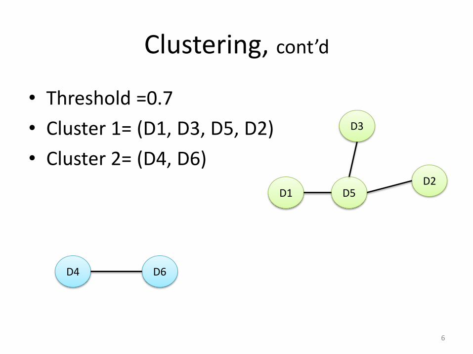
• Threshold =0.7

• Cluster 1= (D1, D3, D5, D2)

• Cluster 2= (D4, D6)

D5 D1 D2

D3

D4 D6

6

Hierarchical Clustering

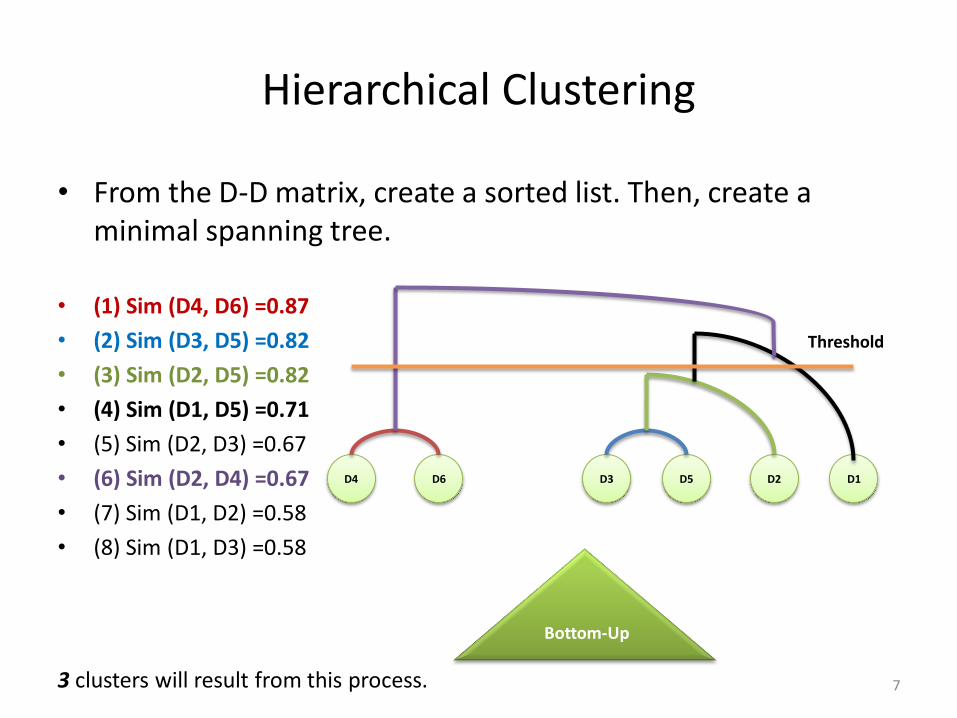
• From the D-D matrix, create a sorted list. Then, create a minimal spanning tree.

• (1) Sim (D4, D6) =0.87

• (2) Sim (D3, D5) =0.82

• (3) Sim (D2, D5) =0.82

• (4) Sim (D1, D5) =0.71

• (5) Sim (D2, D3) =0.67

• (6) Sim (D2, D4) =0.67

• (7) Sim (D1, D2) =0.58

• (8) Sim (D1, D3) =0.58

D4 D6 D3 D5 D2 D1

Threshold

Bottom-Up

3 clusters will result from this process. 7

Cluster Validity

λ- measure

• The document collection is considered a weighted graph.

• λ measures the weighted partial connectivity of the graph.

8

Cluster Validity, λ- measure

• Let C= { C1, C2, ……, Ck } a set of clusters resulted from (say hierarchical clustering).

• λ (C)= 𝐶𝑖𝑘𝑖=1 . λi

• Where λi designates the weighted edge connectivity.

9

Cluster Validity, λ- measure

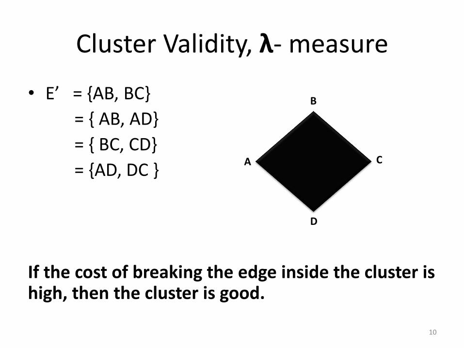
• E’ = {AB, BC}

= { AB, AD}

= { BC, CD}

= {AD, DC }

If the cost of breaking the edge inside the cluster is high, then the cluster is good.

B

A C

D

10

Example

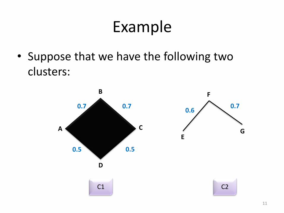
• Suppose that we have the following two clusters:

B

A C

D

F

G E

0.6 0.7 0.7 0.7

0.5 0.5

C1 C2

11

Example, cont’d

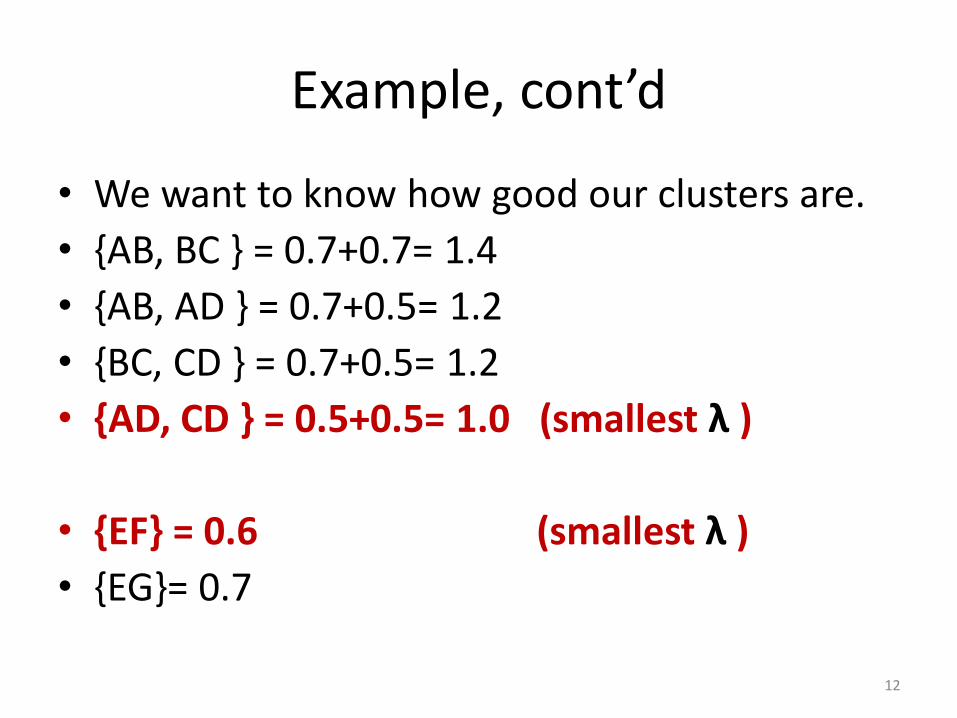
• We want to know how good our clusters are.

• {AB, BC } = 0.7+0.7= 1.4

• {AB, AD } = 0.7+0.5= 1.2

• {BC, CD } = 0.7+0.5= 1.2

• {AD, CD } = 0.5+0.5= 1.0 (smallest λ )

• {EF} = 0.6 (smallest λ )

• {EG}= 0.7

12

Example, cont’d

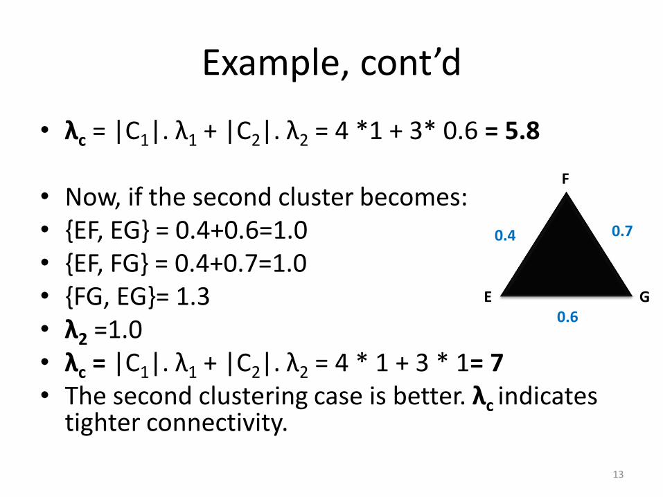
• λc = |C1|. λ1 + |C2|. λ2 = 4 *1 + 3* 0.6 = 5.8

• Now, if the second cluster becomes: • {EF, EG} = 0.4+0.6=1.0 • {EF, FG} = 0.4+0.7=1.0 • {FG, EG}= 1.3 • λ2 =1.0 • λc = |C1|. λ1 + |C2|. λ2 = 4 * 1 + 3 * 1= 7 • The second clustering case is better. λc indicates

tighter connectivity.

F

0.7

E G

0.4

0.6

13

More into Clustering

14

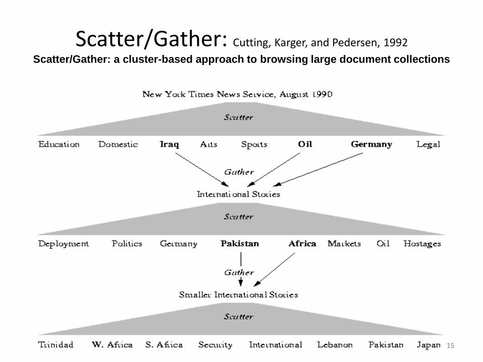
Scatter/Gather: Cutting, Karger, and Pedersen, 1992

Scatter/Gather: a cluster-based approach to browsing large document collections

Sec. 16.1

15

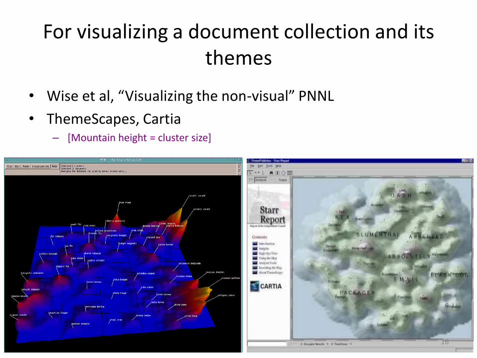
For visualizing a document collection and its themes

• Wise et al, “Visualizing the non-visual” PNNL

• ThemeScapes, Cartia – [Mountain height = cluster size]

16

Why Clustering?

18

For improving search recall

• Cluster hypothesis - Documents in the same cluster behave similarly with respect to relevance to information needs

• Therefore, to improve search recall:

– Cluster documents in corpus a priori

– When a query matches a document D, also return other documents in the cluster containing D

• Hope if we do this: The query “car” will also return docs containing automobile

– Because clustering groups together (documents containing car with those containing automobile).

Why might this happen?

Sec. 16.1

19

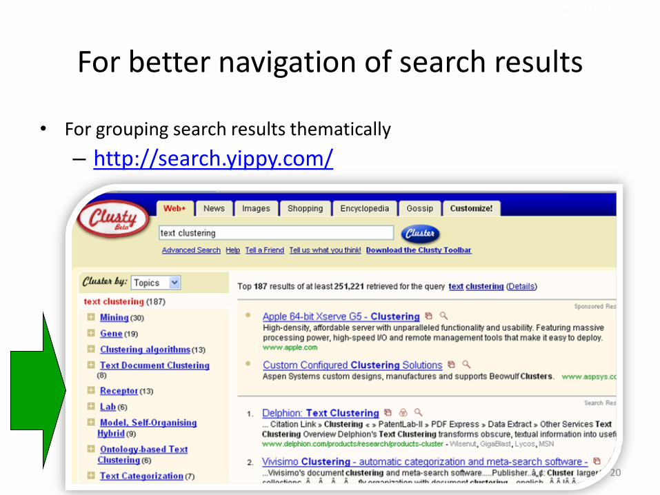
For better navigation of search results

• For grouping search results thematically

– http://search.yippy.com/

Sec. 16.1

20

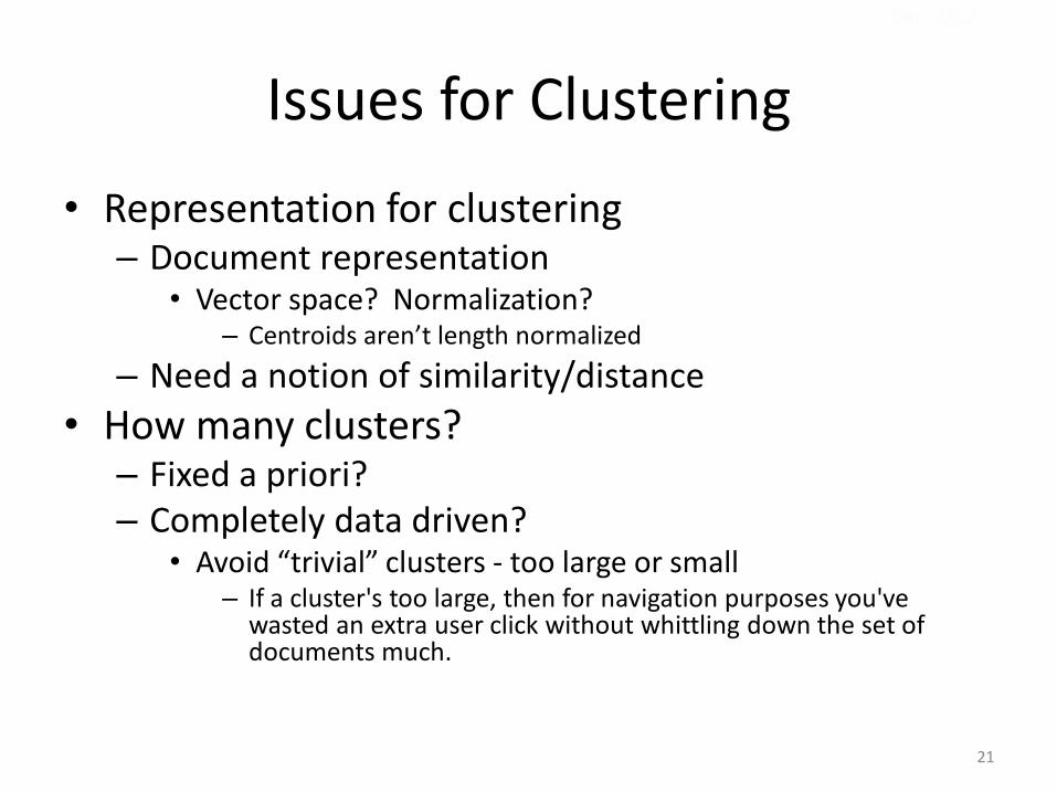
Issues for Clustering

• Representation for clustering – Document representation

• Vector space? Normalization? – Centroids aren’t length normalized

– Need a notion of similarity/distance

• How many clusters? – Fixed a priori? – Completely data driven?

• Avoid “trivial” clusters - too large or small – If a cluster's too large, then for navigation purposes you've

wasted an extra user click without whittling down the set of documents much.

Sec. 16.2

21

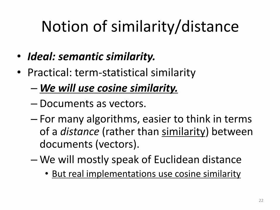
Notion of similarity/distance

• Ideal: semantic similarity.

• Practical: term-statistical similarity

– We will use cosine similarity.

– Documents as vectors.

– For many algorithms, easier to think in terms of a distance (rather than similarity) between documents (vectors).

– We will mostly speak of Euclidean distance • But real implementations use cosine similarity

22

Clustering Algorithms

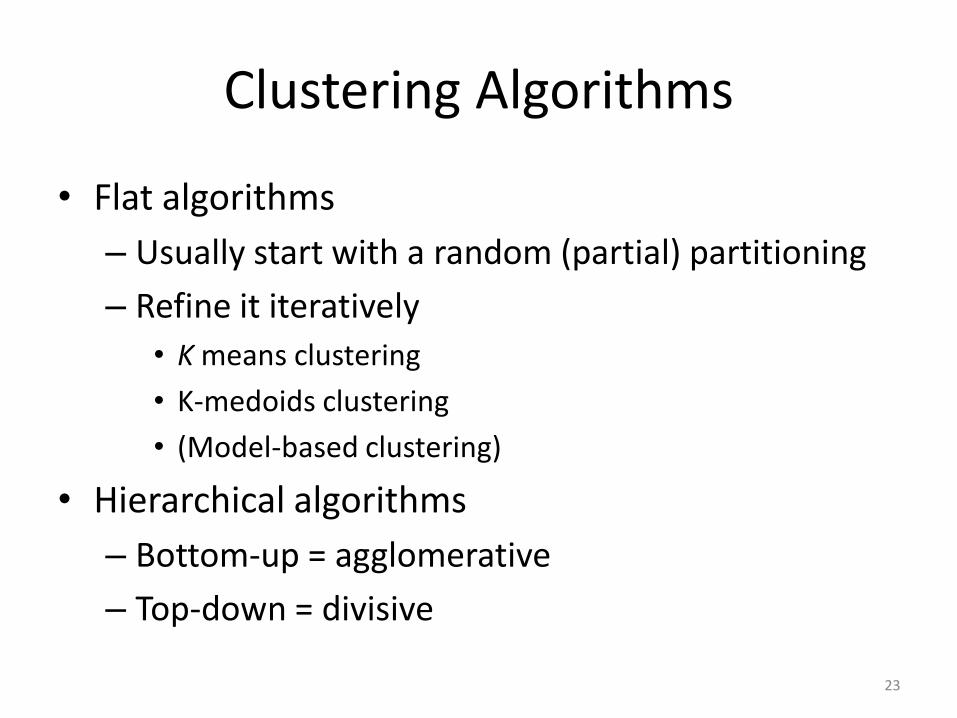
• Flat algorithms

– Usually start with a random (partial) partitioning

– Refine it iteratively

• K means clustering

• K-medoids clustering

• (Model-based clustering)

• Hierarchical algorithms

– Bottom-up = agglomerative

– Top-down = divisive

23

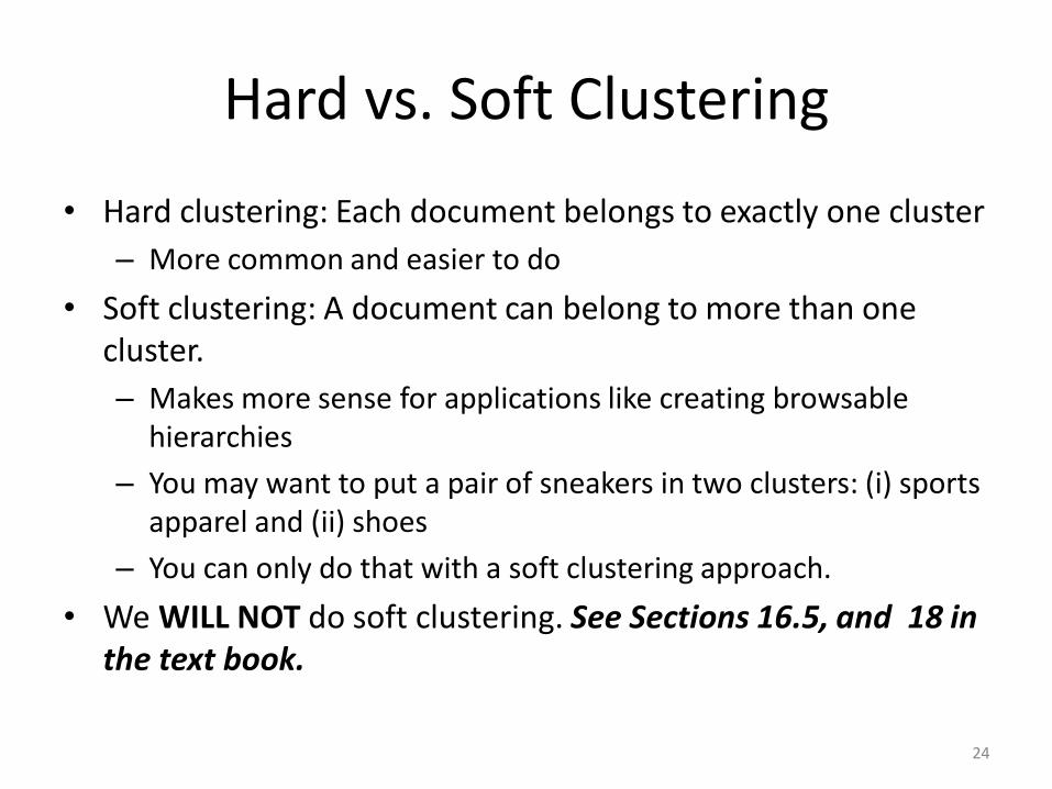
Hard vs. Soft Clustering

• Hard clustering: Each document belongs to exactly one cluster

– More common and easier to do

• Soft clustering: A document can belong to more than one cluster.

– Makes more sense for applications like creating browsable hierarchies

– You may want to put a pair of sneakers in two clusters: (i) sports apparel and (ii) shoes

– You can only do that with a soft clustering approach.

• We WILL NOT do soft clustering. See Sections 16.5, and 18 in the text book.

24

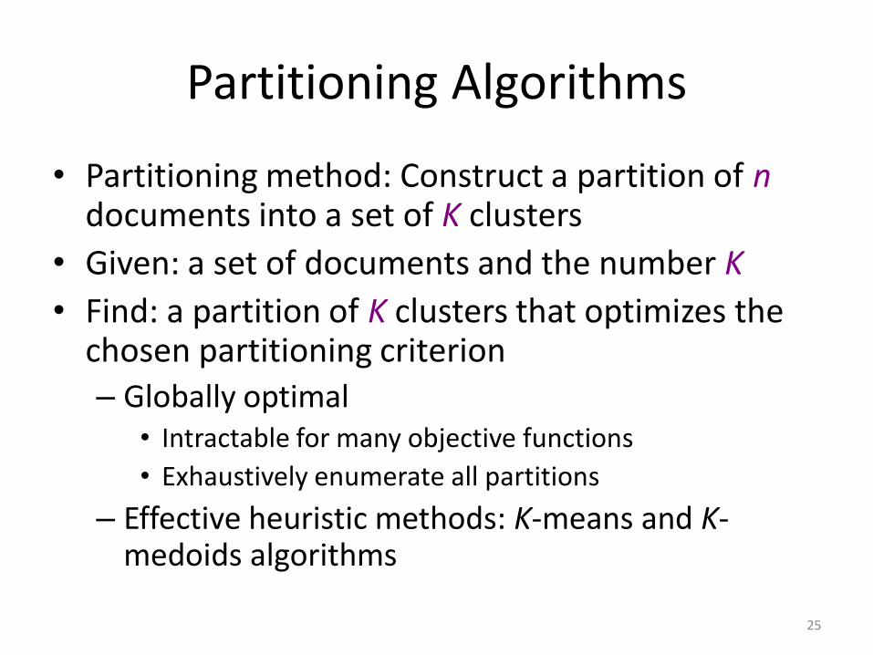
Partitioning Algorithms

• Partitioning method: Construct a partition of n documents into a set of K clusters

• Given: a set of documents and the number K

• Find: a partition of K clusters that optimizes the chosen partitioning criterion – Globally optimal

• Intractable for many objective functions

• Exhaustively enumerate all partitions

– Effective heuristic methods: K-means and K-medoids algorithms

25

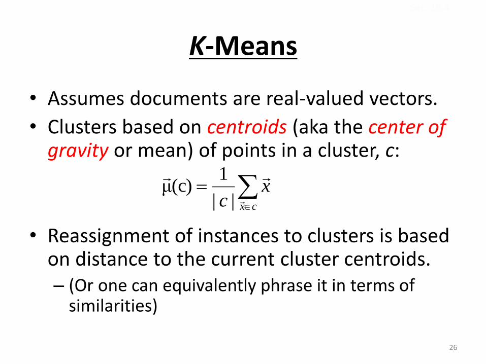
K-Means

• Assumes documents are real-valued vectors.

• Clusters based on centroids (aka the center of gravity or mean) of points in a cluster, c:

• Reassignment of instances to clusters is based on distance to the current cluster centroids. – (Or one can equivalently phrase it in terms of

similarities)

cx

xc

||

1(c)μ

Sec. 16.4

26

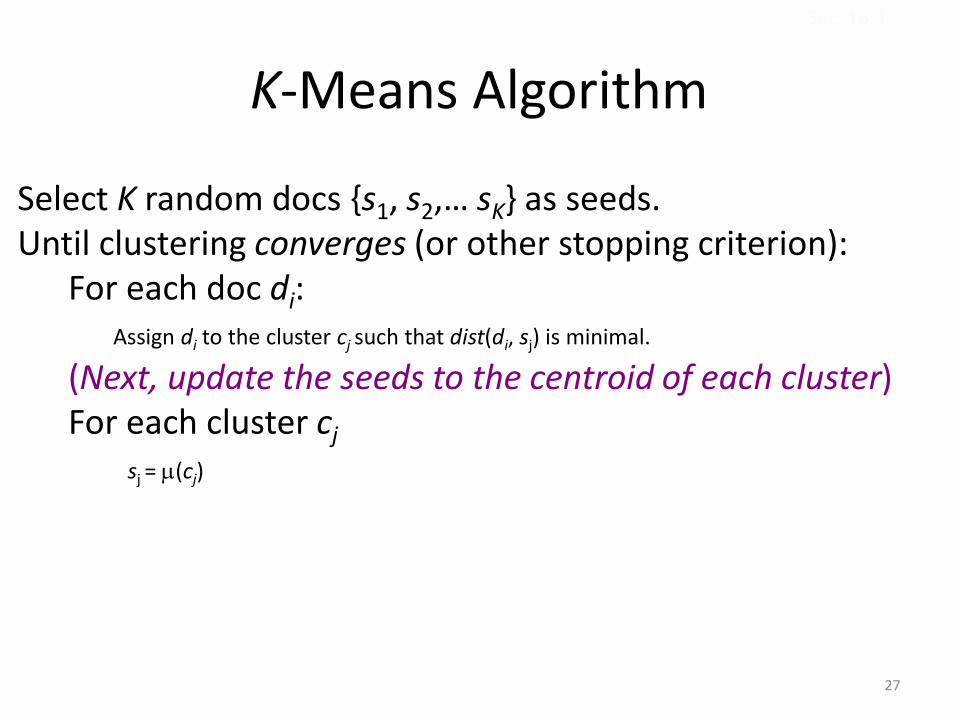
K-Means Algorithm

Select K random docs {s1, s2,… sK} as seeds. Until clustering converges (or other stopping criterion): For each doc di: Assign di to the cluster cj such that dist(di, sj) is minimal.

(Next, update the seeds to the centroid of each cluster) For each cluster cj sj = (cj)

Sec. 16.4

27

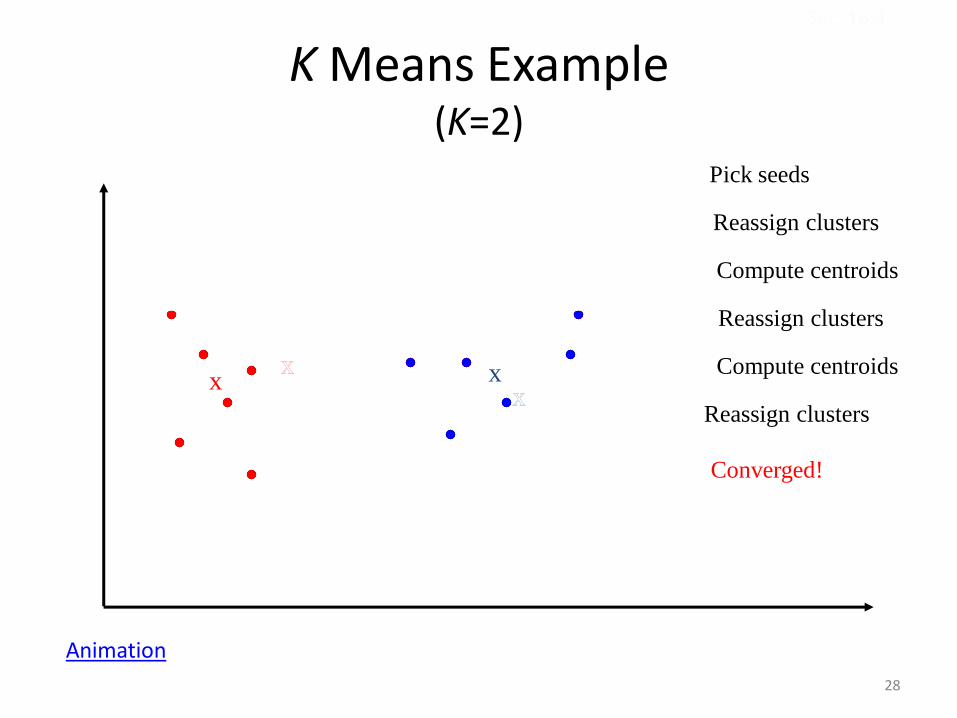
K Means Example (K=2)

Pick seeds

Reassign clusters

Compute centroids

x

x

Reassign clusters

x

x x x Compute centroids

Reassign clusters

Converged!

Sec. 16.4

28

Animation

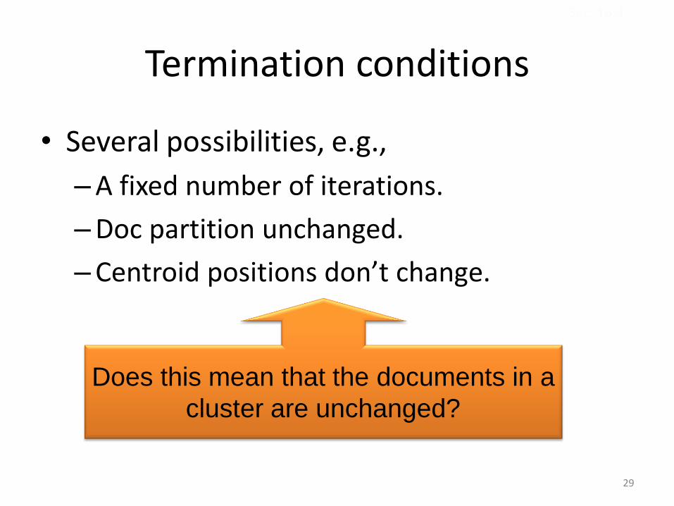
Termination conditions

• Several possibilities, e.g.,

–A fixed number of iterations.

–Doc partition unchanged.

–Centroid positions don’t change.

Does this mean that the documents in a

cluster are unchanged?

Sec. 16.4

29

K-means

• A simple demo showing k-means iterations

• http://home.dei.polimi.it/matteucc/Clustering/tutorial_html/AppletKM.html

K-medoids

• Similar to k-means

• Instead of a centroid, the choice goes to a document as the center of gravity (a medoid).

• More robust to noise and outliers as compared to k-means.

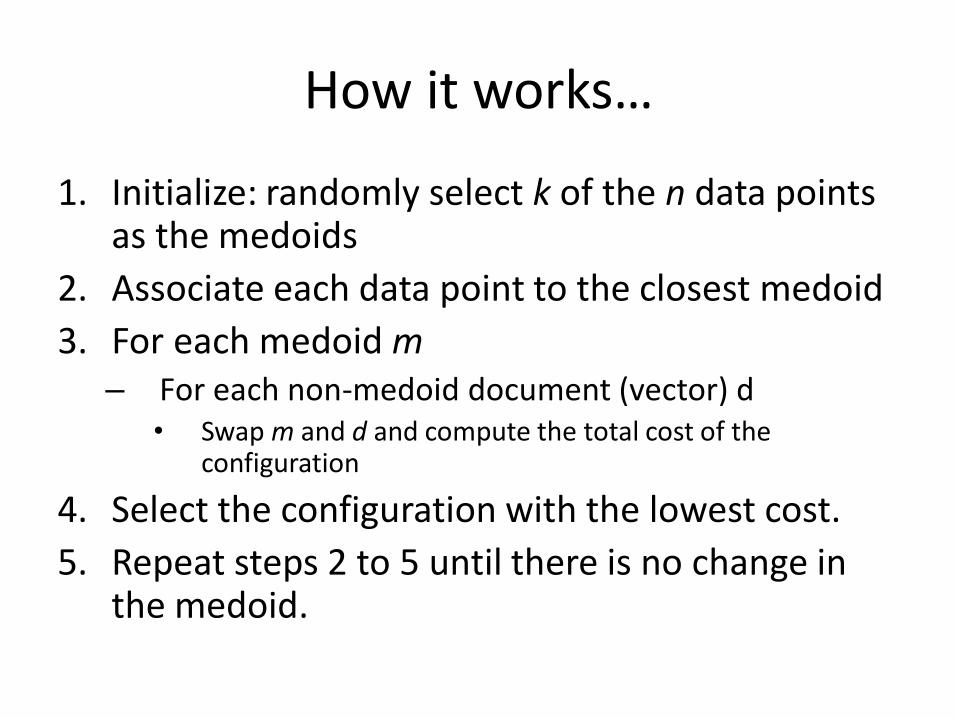
How it works…

1. Initialize: randomly select k of the n data points as the medoids

2. Associate each data point to the closest medoid

3. For each medoid m – For each non-medoid document (vector) d

• Swap m and d and compute the total cost of the configuration

4. Select the configuration with the lowest cost.

5. Repeat steps 2 to 5 until there is no change in the medoid.