ClusterSculptor: A Visual Analytics Tool for High-Dimensional Data

Eun Ju Nam1 Yiping Han1 Klaus Mueller1 Alla Zelenyuk2 Dan Imre3

1Stony Brook University 2Pacific Northwest National Lab 3Imre Consulting

ABSTRACT Cluster analysis (CA) is a powerful strategy for the exploration of high-dimensional data in the absence of a-priori hypotheses or data classification models, and the results of CA can then be used to form such models. But even though formal models and classifi-cation rules may not exist in these data exploration scenarios, domain scientists and experts generally have a vast amount of non-compiled knowledge and intuition that they can bring to bear in this effort. In CA, there are various popular mechanisms to generate the clusters, however, the results from their non-supervised deployment rarely fully agree with this expert knowledge and intuition. To this end, our paper describes a comprehensive and intuitive framework to aid scientists in the derivation of classification hierarchies in CA, using k-means as the overall clustering engine, but allowing them to tune its parameters interactively based on a non-distorted compact visual presentation of the inherent characteristics of the data in high-dimensional space. These include cluster geometry, composition, spatial relations to neighbors, and others. In essence, we provide all the tools necessary for a high-dimensional activity we call cluster sculpting, and the evolving hierarchy can then be viewed in a space-efficient radial dendrogram. We demonstrate our system in the context of the mining and classification of a large collection of millions of data items of aerosol mass spectra, but our framework readily applies to any high-dimensional CA scenario. Keywords: Visual Analytics, High-Dimensional Data, Visual Data Mining, Visualization in Earth, Space and Environmental Sciences. Index Terms: I.3.8 [Computer Graphics]: Applications.

1 INTRODUCTION Clustering is the process of partitioning a collection of data points into separate groups, according to some measure of similarity. The term cluster analysis (CA) was first used by Tryon [20] and encompasses a number of different algorithms and methods to achieve this goal. CA can be utilized to discover associations in high-dimensional (N-D) data without a prior model or classifica-tion rules - the structures are discovered as the clustering proceeds. Hence, there is high potential for discovering unexpected associations. The so evolved hierarchy can then be labeled by the user and the decision boundaries be used for a more informed separation of a future data collection of similar nature. In this respect, CA can be considered a learning mechanism [16].

The result of CA is usually a hierarchy, with intra-cluster simi-larity decreasing towards the root. There are a number of metrics for measuring the similarity among two separate clusters [13], such as the distance of the two closest points in the two clusters

(single linkage), the distance of the two furthest points (complete linkage), or the average distance between all pairs of points in the two clusters (un-weighted pair-group average), and others. Ward has proposed a different approach based on the analysis of variance (ANOVA) to evaluate the distances between clusters [23]. In fact, the distance measure used has a great effect on the shape of the aggregated clusters. For example, the single-linkage scheme tends to create long and stringy clusters, while Ward’s method generates many clusters of small size. However, these data aggregation preferences may not always match the true hierarchical organization of the data, particularly not when there are close ties which are nevertheless rejected due to these purely algorithm-driven choices. Clearly more intelligence is needed in the clustering process, which, however, is not available in encapsulated form - by the very definition and nature of CA. On the other hand, injecting live expert input and intuition into an ongoing analysis process is one of the main motivations behind visual analytics. By taking advantage of this non-compiled domain expertise one can non-linearly steer the CA into a more favorable constellation. In order to make this undertaking as effective as possible, the expert must gain a comprehensive picture of both the data and the current status of the process. Our work proposes a highly visual framework to accomplish this, with a strong emphasis on conveying as much of the structure of the data as possible, in non-overwhelming ways.

The opportunities gained from involving users into a classifica-tion and aggregation task has been recognized in a number of recent works in the KDD (Knowledge Discovery and Data mining) community, such as [1][25], and has been quite successful. In many cases these works offer some visual support, mostly in form of 2D plots or 3D height fields, to allow users to cast the final decision in defining the cluster boundaries and separations, which can be non-trivial in the presence of noise and ambiguities. Many of these approaches perform a number of trials, performed with different clustering parameter settings, and the system described in [8] offers a convenient glyph-based summary matrix to visualize the gist of these trails, both for refinement and for selection. None of these systems attempts to visually convey the N-D space all at once – only the result of (iterative) projections into a displayable space (2D/3D) is shown. On the other hand, systems such as parallel coordinates [11] and star coordinates [12] offer visual frameworks that allow users to interactively and directly explore these high-dimensional spaces, either just for data viewing or to isolate existing clusters and build hierarchies. However, the curse of dimensionality can pose limits to both of these approaches relatively early. In the projection approaches, the iterative sub-space projections from N-D to 2D/1D and the associated growth in the number of required trials makes high data dimensionality of, say, greater than 100 difficult. On the other hand, the visual coordinate displays require a sufficient amount of screen space per dimension, which also imposes limits. A suitable way to deal with this problem is to use a space-efficient pixel map for data display and/or principal component analysis (PC) or other related techniques for dimension reduction.

1email: {ejnam, yiping, mueller}@cs.sunysb.edu 2email: alla.zelenyuk@pnl.gov 3email: dimre2b@charter.net

An important goal when dealing with visual interaction techniques, in which experts are asked to apply their domain knowledge, must be the interpretability of the displayed information. This is where dimension reduction can cause problems since these types of techniques often rotate or warp the data into a new axis system where the relationship of data vector values to the original data attributes is difficult to discern.

The domain application for which our system has been developed is atmospheric science, where the data is composed of 450-dimensional mass spectra of aerosol particles acquired by a state-of-the-art SPLAT (Single Particle Laser Ablation Time-of-Flight) mass spectrometer [26]. The goal is to employ clustering as a mechanism to learn the composition of particles for subsequent automated classification of new particle acquisitions, using the learnt spectra hierarchy. In addition, the classification hierarchies so obtained are novel in their own right, producing new insights in the compositions of aerosols, which are influenced by climate, pollution, and other factors. Thus with the domain expert tightly integrated into the visual analytics loop, such a clustering system must allow a data-oriented information display and manipulation, in the presence of very high-dimensional data. This setting rules out a direct use of PCA, while the high data dimensionality requires a pixel-map display and makes an iterative projection framework less attractive. Our paper describes such a framework, meeting all of these design goals. Our system provides a variety of interaction capabilities that allows experts to delineate clusters virtually in N-D space – a process which we refer to as cluster sculpting and N-D viewing.

Our paper is structured as follows. In Section 2, we will discuss existing related work, Section 3 presents an overview of our system, and Section 4 outlines the system components. Section 5 describes our domain application in more detail and then shows the system in action. Finally, Section 6 ends with conclusions and an outlook onto future work.

2 RELATED WORK In addition to the more clustering-oriented works already mentioned in the introduction, much research has been published on the visualization of N-D data. One way to distinguish these methods is by the strategy they use to overcome the problems that arise from the limited dimensions available for display. Pixel-based techniques [14] create an N×N matrix of scatter plots in which each coordinate pairing is displayed, while force-directed methods and multi-dimensional scaling have been employed to “flatten” the N-D space into 2-D [4][15][17]. On the other hand, Star Coordinates (SC) [12], Parallel Coordinates (PC) [11], and RadViz [9] flatten the axes of the N-D space into 2D. While in PC an N-D data point reduces to a piecewise linear curve, in SC and RadVis, an N-D point reduces to a 2D point whose coordinates are given by the average coordinate value in the multi-spoke radial coordinate system. In the latter, due to the averaging points distant in N-D may still fall into a small region in 2-D, which requires a closer inspection of the points before cluster assignment. A survey of these techniques is presented in [5].

Both Parallel Coordinates and Star Coordinates have been extended into interactive clustering applications [19]. The reduction of the data into a 2D scatter plot (an arrangement of lines in Parallel Coordinates, an array of dots in Star Coordinates) can cause points or lines to be obscured (overdrawn) by other such elements, but various strategies exist, such as zooming, brushing [6], axis reordering [18], and filtering [3], to alleviate these problems. Fisheyes and hierarchical brushing [6] can be employed to make the display scalable.

The capability of allowing expert users to guide the clustering (also called semi-supervised clustering) has been promoted by [22][25] and others. Kreuseler and Schumann [15] use a similarity matrix in conjunction with a bottom-up approach to create a binary tree. They then cluster the nodes of this tree by ways of a user-defined discrete 1-D heterogeneity scale acting on the computed similarity measures at each node. In contrast, our system takes this interaction mechanism a step further by allowing users to influence the similarity weights directly in N-D space, in an implicit manner via our data-centric interface. This allows an earlier control over the composition of the generated clusters, which is desirable for larger N (Kreuseler used the car data base where N=6). Similar to Kreuseler [15] and Wilson [24], we also use a radial dendrogram to display our hierarchy in a space-efficient manner by placing the root into the center. But our approach tightly integrates the dendrogram into the clustering framework. Users are able to move and re-cluster nodes within the hierarchy.

3 OVERVIEW The main idea of our system is that while there are many clustering algorithms, none will give a one-size-fits-all result. It is ultimately only the domain expert who can identify suitable clusters, and our system aims to provide an effective visualization and manipulation framework for this. First, a set of first-guess clusters is presented to the user who then can merge, split, and re-organize these clusters using his expert knowledge, intuition, and domain requirements. The ultimate goal is to learn the clustering rules from these examples, which will then provide a better pre-clustering for future datasets to minimize further tuning, and enable eventually real-time automated classification.

Hierarchical clustering can be conducted in a top-down or bot-tom-up fashion. In a top-down approach the data space is continu-ously subdivided into sub-clusters until further subdivision of an individual cluster is no longer meaningful (by some metric or user decision), while the bottom-up approach starts with the collection of isolated data points and continuously merges them until the single (root) cluster is obtained [7]. The top-down approach is typically more intuitive and also faster, since it allows one to stop once all sub-clusters have reached non-divisible group status. The SPLAT device can easily acquire 100s of thousands of particles in a single session. Therefore, in order to reduce the data, we use an initial automated and reasonably fine-grained bottom-up pre-clustering for data reduction (similar to [28]), but then switch to a more refined top-down strategy supervised by the user (this stage is described in this paper). The data size at this stage is on the order of 100s to 10,0000s of data points. The scientist uses the system to carefully cluster the sample dataset, creating the hierarchy. Here, the clustering algorithm (k-means, single-link, complete-link, and CURE [7]) that is applied can be user-specified at every level of the hierarchy, and various linked visualizations are provided to monitor the shape of the clusters as well as the composition of the hierarchy. In addition, clusters can be reshaped and regrouped at any time. Once the classification hierarchy is defined over the sample dataset, the entire collection of data points is classified using the rules learnt from this training session, yet outliers will also be presented to make sure nothing is missed. Support-vector machines (SVM) [21] are then used to encode and learn these rules.

4 SYSTEM COMPONENTS We now introduce the system components, while Section 5 will show these in context of an actual clustering session. The overall

interface is depicted in Figs. 1-3 (note that Figs. 1, 2, and 3 are screen captures taken at different stages of the classification to enable depiction of all functionalities), with the labels indicating the various components, as described as follows.

4.1 The Point Map The Point Map displays each data vector (the mass spectrum) as a horizontal line of colored pixels, one per axis direction. The color mapping is according to value, normalized from 0 to 1, and the color is mapped from blue to red. The point lines are grouped by the smallest cluster they are in (the leaf nodes of the hierarchy). Within each cluster, the points are sorted by their distance to the center of the cluster, but users can also sort the points by value in the particular dimension or by particle sizes.

The user may double-click on any such cluster to make it the active cluster. The histogram window and the PC window then display the information of this active cluster. The user may click on any particle to set the initial cluster center for k-means.

When the k-means clustering iterations terminate, it is possible that some of the sub-clusters only have a very small number of points. These points would be considered as outliers, but should not be discarded as they may be the kind of rare gemstone-type information the scientists is looking for. We collect these outliers into a special cluster which we call odd-lots to bring these points to the user’s attention.

4.2 The Dendrogram The dendrogram represents the current status of the cluster hierarchy. It is a flat version of the radial dendrogram of SpectraMiner (see Fig. 3 and the description in Section 4.7). When the mouse pointer is over the point map, the (neighbor) cluster closest to the data point under the mouse is emphasized in the dendrogram as a blue box. On the other hand, when the user moves the mouse pointer over a leaf cluster in the dendrogram, its

nearest neighbor cluster is emphasized. Finally, the user can also merge or move clusters by selecting nodes in the dendrogram.

4.3 The Neighbor Map This window is designed to show the neighborhood relations between data points or clusters. Two modes are associated with this window. The first mode is the neighbor mode. As mentioned above, when the mouse pointer is over the point map, the neighbor leaf-cluster closest to the point is emphasized in the dendrogram. In addition, the distances of all data points to the cluster center of the emphasized cluster are illustrated in the neighbor map as bar length. Each bar has one of three colors, green, blue, and red. The currently active data point is rendered in red, while the points with green bars have the same neighbor than the current data point. In other words, their nearest neighbor is the one that is shown emphasized in the dendrogram. Points with other neighbors have blue bars in the neighbor map. This information can be helpful to discover points that are incorrectly classified or some patterns of clusters. Also, it helps to better picture cluster relationships in N-D space. Moving the mouse around to dynamically change the neighborhood map in many cases reveals useful information.

The second mode is the particle size mode (not shown here) where the measured size of the particle can also be displayed in form of a (vertical) 1D plot. The user may then sort data points by particle size which is often helpful.

4.4 The Histogram Window The histogram displays the density values of each dimension. The x-axis is the dimension number. For the y-values, we sum up all values for each dimension and then normalize from 0 to 255. The users can set weights to particular dimensions to compress or stretch the cluster in N-dimensional space along the cluster axis. This gives rise to a weighted k-means effect. The user can select to see either the original histogram or the weighted histogram.

Figure 1. The ClusterSculptor interface

Figure 2. EigenMap with SVM plane and major dimensions.

Once the user changes the weights in this histogram, the PCs are recomputed according to the new weights and displayed in the PC window (described next).

4.5 The Principal Component (PC) Window The PC window shows the first principal component as a default. The first PC represents the axis along which the variance of the dataset is the greatest, that is, the first PC has the greatest eigenvalue.

The user may choose what to display in this window, either eigenvectors or eigenvalues. The user may also select other principal components to be displayed instead of the first PC. In Fig. 1 the dot products of the first PC and the individual axes are shown (blue is positive and green negative). The longest bar indicates the axis of greatest alignment.

Our system provides an option to scale the PC by the histogram. This is shown in Fig. 5A. Here, we show (top to bottom) the histogram, the point map, the three largest PCs, and the eigenvalues. We observe that none of the major PC axis dimensions (the data axes of greatest alignment) has significant activity in the actual dataset. Both the histogram and the point map show that there are not many values along these dimensions (recall that blue encodes a value of zero). In order to adjust for this situation, we allow the user to scale the PC by the histogram. The new configuration is shown in Fig. 5B. This rescales the space along these directions, yielding tighter clusters. Note that this operation creates a standardized rescaling compared to the more user-controlled re-scaling facilitated by weighting the histogram. Finally, the scaling is also helpful for the EigenMap discussed in the next section.

4.6 The Eigen Map The point map is useful for comparing the N-D vectors on a per-component basis. However, this plot does not convey the spatial relationships very well. The neighbor map was intended to illustrate these spatial relations better, but it still lacks the immersive effects of a true 3D display. We can use the PCs to create such an illustration. Let us take the three PCs with the largest eigenvalues and project our dataset onto these PC axes. Since the PCs represent the most variant axes in N-D space (usually the eigenvalues decay fast), we can perceive clusters more easily, in this, what we call EigenSpace. This display is shown in Fig. 2 below and the color of the points displayed corresponds to the leaf node’s color in the dendrogram (the EigenMap shows the point cloud of the active cluster). Finally, in order to ground the user in the true data space, we project into this PC-based coordinate system the closest data dimension axes. Such a projection is found by taking the dot product of the axis vector with each PC vector.

As mentioned in the previous section, the best depiction of the space’s occupancy is obtained by first weighting the PCs with the histogram and using these to construct the EigenMap. This in turn also creates a more significant projection of the true data axes. Recall that in Fig. 5B we identified dimension axes 62, 30, and 81 as the axes most aligned with the weighted PCs and therefore most associated with data variations in the cluster. These are drawn in blue into the EigenMap cube of Fig. 2. Finally, we can

also project the hyper-plane optimally separating the clusters (once it is classified) and computed via SVM.

4.7 Cluster Information Window Our interface provides a variety of information and selection options beside the display area. The first such panel is the Cluster Information Window. There, the user can view all information with regards to the active cluster, active data point, and active dimension as well as other necessary attributes. This window also shows information about every dimension axis. In the second panel, the users may choose various display options, what information to display or not, etc. In the third panel the user can control the classifier itself: set weights, the threshold, the number of the cluster center, and so on. The next panel controls the EigenMap, and the last panel allows for managing the dimensions. Here, the user may create a new dimension or sum several dimensions which the expert considers to be conjunctively related. This function highly depends on the user’s prior knowledge and intuition and influences the clustering in an expert-driven way.

4.8 SpectraMiner Finally, SpectraMiner (see Fig. 3) presents the current state of the classification in an interactive hierarchical circular dendrogram. In addition to this display, SpectraMiner offers the user a wide range of additional tools which have been described in [10][27]. Initially, SpectraMiner holds the results from the non-supervised pre-clustering, and the initial hierarchy is created by using one of the similarity metrics mentioned in the introduction. The user then selects a sub-branch (or the entire hierarchy) and ports it to ClusterSculptor for closer visualization and refinement.

Figure 3. The SpectraMiner interface.

5 VISUAL ANALYSIS EXAMPLE In this section we illustrate our system in greater detail, using a real visual analytics session (enumerated in Fig. 5) as a demonstration example. We begin with describing our domain application in greater detail, motivate the move to the interactive clustering or cluster refinement environment described here, and then show the sequence of actions associated with this task, richly illustrated.

5.1 Domain Application SPLAT [26] is a single particle mass spectrometer that is used to characterize the properties of ambient atmospheric particles in real-time. These particles impact our climate, and when inhaled our health. They are found to have a wide a range of sizes and to be composed of a large number of substances. Because the impact

of atmospheric particles on public health and on climate strongly depend on their compositions and sizes it is important to know these quantities in great detail. SPLAT is capable of measuring the size and composition of 20 particles per second in while sampling ambient air directly. It records, for each particle the time of detection particle size and a mass spectrum consisting of signal amplitudes of 450 mass units. The relative intensities of these 450 amplitudes carry the pertinent information to identify the particle’s composition. During typical field deployments SPLAT operates 24 hours per day recording millions of data points.

SPLAT is also designed to detect airborne bacterial and viral warfare agents whose concentrations are expected to be extremely low. In this application, the success depends on timely high precision detection and identification of rare events that is embedded in a vast amount of data/background.

The goal is to employ the overall system as a mechanism to learn the composition of particles for subsequent automated classification of new particle acquisitions, using the learnt spectra hierarchy. In addition, the classification hierarchies so obtained are novel in their own right, producing new insights in the compositions of aerosols, which are influenced by climate, pollution, and other factors.

5.2 Motivation Our experience with SpectraMiner most often reveals that the statistically based classification results are not satisfying. It is common to find at the completion of the clustering process that particles of identical compositions were separated into a number of different classes and that particles of different compositions reside in the same cluster. Yet to the expert’s trained eye, the mass spectra contain sufficient information to accomplish a proper classification. An expert’s view of the data reveals that in the vast majority of the cases typical clustering problems that are found could have been avoided were it possible for the expert to input his/her knowledge to steer the classification into the proper conclusion.

Example: In single particle mass spectrometry it is not uncommon to find cases in which one of the substances is contained in a number of particle types, which otherwise are significantly different. If that substance happens to produce a high amplitude signal in the mass spectrum every one of the particle types that contain that substance are most often found to be jointly clustered. This is a result of the fact that the few high-amplitude coordinates tend to dominate the classification process, while the low amplitude peaks that could have been used to differentiate between particle types are in essence ignored. Sodium and potassium are two alkali metals that are commonly found in a number of atmospheric particle types. The presence of even a small amount of alkali metals produces very high signal intensities making proper classification difficult.

Fig. 4(a) presents a screen capture of the SpectraMiner dendrogram of data generated from 36,000 lab generated particles. To produce this hierarchy, we use an off-line k-means clustering. Here we focus on nodes A and I composed of clusters 1, 2 and 50 to 57 respectively. Node A represents two types of sodium containing particles sodium nitrate (SN) and sodium chloride (SC) and node I includes three types of organic compounds, lauric acid (LA), pyrene (PY) and exhaust soot. These classes contain substances that are commonly found in atmospheric particles. Fig. 4(b) shows the content of the 9 clusters these data were classified into, clearly illustrating the difficulties mentioned earlier. In the following we show how this can be remedied, via cluster sculpting. Both the A-node and the I-node in Fig. 4(a) will be refined.

Figure 4. (a) A dendrogram of 36,000 laboratory generated individual particle mass spectra. The data were classified into 61 clusters are presented here in a circular hierarchical tree format. The two nodes and the 9 clusters that are the subject of this paper are identified and marked. (b) Bar graph showing the content of the 2 nodes and 9 clusters that are being re-clustered in this paper. In node A the most of the two sodium containing particles are in clusters 1. In node I 3 types of carbon containing were separated into 7 clusters one of which is strongly mixed.

5.3 A-Node Cluster Sculpting Fig. 5A shows the 6,000 two sodium containing particle types. The major dimensions from each three PCs do not have many values in the point map and the histogram. So we can assume that they are not important dimensions, even if there is a big variance along those dimensions. We also see that there are only 3-4 significant eigenvalues, which means that the first three PCs represent the sub-space quite well.

Next, for the reasons stated above, the expert seeks to reduce the role that sodium (the largest peak) plays in the classification of the node. Therefore, he sets the weight of this dimension to 0.01. Following, he scales the PCs by the histogram. Now only the major dimensions in the PCs are active in this adjusted space (see Fig. 5B).

Fig. 5C shows the EigenMap of the cluster with the data axes for element 30, 81, and 62. From this display the somewhat irregular shape (two arms, with one having a kink) of the cluster becomes apparent.

Now an attempt is made to classify, via k-means, the node into two clusters. The result is shown in Fig. 5D. The result is less than satisfactory. Next, Fig. 5E shows the outcome when 5 k-means seeds are used and we see that this classifies well. However, the pink node is still misclassified here. It should really been divided into two separated clusters.

Fig. 5F takes a closer look at the pink node, making it the active cluster. In the associated PC setting, the 24th data dimension emerges as a major dimension for all three PC coordinates, indicating that the points are highly correlated with the 24th element in the mass spectrum. This strong impact of this element on the classification can be overcome by setting the weight for the 24th dimension to 0.05. This allows a projection into another subspace, shown in Fig. 5G, where the element dimension pointed to by the brown arrow is the main direction. We can now easily see two different types of clusters in this pink node. We also see that there are two different types of clusters in the point map. Sorting the point map along the main element dimension allows a fairly good differentiation of these two clusters.

Next we examine the interplay of neighbor map, point map, and EigenMap. Fig. 5H (a) shows the EigenMap of the whole dataset. Fig. 5H (b) has the mouse pointer traveling over the bottom half of the data points (note, the red line in the neighbor map is the current data point). We see that the purple node is the nearest neighbor (highlighted in the dendrogram on the bottom) for the current data point – this part is the portion marked by a rectangle

A. 6,000 two sodium containing particle types (A node in Fig 4). The major dimensions from each of the three PCs do not have many values in point map and histogram. Also, there are only 3-4 significant eigenvalues.

B. The expert reduces the effect of Sodium (the largest peak) by setting the weight of this dimension to 0.01. Then the PCs are scaled by their histogram values. Now only the major dimensions in the PCs are active in this adjusted space.

C. EigenMap with new PC coordinates from Fig B. This map shows two separate clusters.

D. Attempt to classify into two clusters using automatic k-means clustering with two centers. It fails.

E. Using automatic k-means clustering with five cluster centers. In general, this classifies well. However, the pink node is mis-classified here. It should be divided into two separated clusters. (a) the dendrogram, (b) the Eigen map.

F. A closer look onto the pink node. Now, the pink node is the active cluster. The 24th dimension is a major dimension for all three PC coordinates.

G. By setting the weight for the 24th dimension to 0.05, other major dimensions emerge in the PC. The EigenMap reveals two different types of

Figure 5. A typical analysis and classification session (continued below)

in the EigenMap. Next, as shown in Fig. 5H (c), when the mouse pointer travels over the top half of the data points, the blue node emerges as the nearest neighbor for the current data point – this part is the circled part in the EigenMap. Now see Fig. 5I for a closer look. There are still some green bars in the upper part of the marked line of neighbor map, but even if those parts are closer to the purple cluster in Euclidean distance, they should belong to the circled part in Fig. 5H. This decision is made when confirming the cluster shapes in the EigenMap display and looking closely at the point map. Fig. 5I (b) is the result of clustering using Fig. 5I (a). Finally, Fig. 5I (c) is the EigenMap of the pink node separated by an SVM plane. We see that the two clusters are divided well.

Fig. 5J shows the entire node after the cluster-sculpting. Now, the active cluster is the whole dataset. Even if there are six

clusters here, we only want to classify into two well-separated clusters. We can merge red, purple, and green into one new cluster. In the same way, we can merge yellow, blue, and orange into one new cluster. Fig. 5K shows the final result after the merging.

Finally, Fig. 5L shows the SVM Plane for the resulting separation, and Fig. 7 (b) left shows the new composition of the re-clustered node A. We see that the compositions of the two clusters are now pure, which means that the refinement procedure just performed has yielded a good classification rule.

Looking at the complex EigenMap shape of the resulting two clusters as well as at the numerical neighborhood map conflict, it is unlikely that automated algorithms would have found this separation, at least not easily.

H. (left) Cooperative displays: neighbor map, point map, and EigenMap (a) EigenMap of the whole dataset. (b) The mouse is traveling over the bottom half of the data points. The red line in the neighbor map is the current data point, and the purple node is the nearest neighbor (highlighted in the dendrogram). These points are contained in the rectangular part in the EigenMap. (c) When the mouse indicates the top half of data points, the blue node is a nearest neighbor for the current data point. This part is contained in the circled part in the EigenMap.

I. (a) Graphical method to classify the data into two clusters. Note there are still some green bars in the upper part of the marked line of neighbor map. But even if those parts are closer to the purple cluster in Euclidean distance, they should belong to the circled part in Fig. 11. This decision is made by the expert, applying his domain knowledge. (b) The result of clustering using (a). (c) EigenMap of the pink node with the SVM plane. The two clusters are divided well.

J. (left) The entire node, viewed after cluster-sculpting. We want to merge these into two well-separated clusters.

K. The final result after merging clusters.

L. (left) Support Vector Machine Plane for the resulting two clusters.

Figure 5. (continued from previous page) A typical analysis and classification session

Figure 6. The result of the classification of the mass spectral data of the carbon containing compounds particles (I node in Fig. 4 (a)) into 3 clusters. This classification used several sculpting techniques by the domain experts. The neighbor map is now in the particle size mode.

5.4 I-node Cluster Sculpting Returning to Figure 4 we note that the I-node represents a case in which particles of the same type were classified into a number of clusters and others were not properly separated. Figure 6 shows the mass spectra of the 5,548 particles that reside in node I. Here the mass spectra are dominated by a relatively high intensity in three coordinates and a classification to achieve complete separation is not possible on the basis of mass spectral intensities alone. In this case we take advantage of our a-priori knowledge of the fact that virtually all exhaust soot particles have a size that is nearly 100 nm. We use the program to sort the particles by size (left vertical panel)

and use that property to identify and isolate 2872 out of the 2916 soot particles in this node. The rest of the data are easily classified once the spectra are sculpted to yield the nearly pure, three clusters shown in Figure 6.

5.5 Exporting to the full hierarchy Once the data have been classified, they are exported back to SpectraMiner where they replace the previously classified data providing the user access to a wide range of data visualization and mining tools. Fig. 7(a) shows the dendrogram with the re-clustered data. In Fig. 7(b), we can see the classification result is much improved over the result shown in Fig. 4(b).

Figure 7. (a) The dendrogram containing the re-clustered A and I nodes. (b) A bar graph showing the content of the clusters as they are imported back into SpectraMiner.

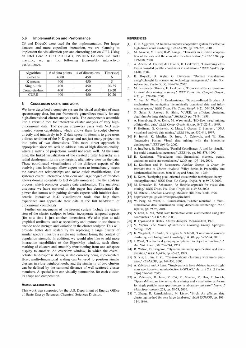
5.6 Implementation and Performance C# and DirectX were used for the implementation. For larger datasets and more expedient interaction, we are planning to implement the visualization part and clustering part on GPU. Using an Intel Core 2 CPU 2.00 GHz, NVIDIA GeForce Go 7400 machine, we get the following (reasonably interactive) performance.

Algorithm # of data points # of dimensions Time(sec)K-means 4000 450 6 K-means 400 450 5

Single-link 400 450 20-25 Complete-link 400 450 15-20

CURE 400 450 10-20

6 CONCLUSION AND FUTURE WORK We have described a complete system for visual analytics of mass spectroscopy data, but our framework generalizes readily for any high-dimensional cluster analysis task. The components assemble into a versatile tool for interactive cluster analysis of very high-dimensional data. The system empowers users with N-D aug-mented vision capabilities, which allows them to sculpt clusters directly and intuitively in N-D data space. It attempts to give users a direct rendition of the N-D space, and not just many projections into pairs of two dimensions. This more direct approach is appropriate since we seek to address data of high dimensionality, where a matrix of projections would not scale well. At the same time, the linked visualization of the created cluster hierarchy in a radial dendrogram forms a synergistic alternative view on the data. These coordinated visualizations of the different aspects of the evolving data landscape allow expert users to immediately assess the carved-out relationships and make quick modifications. Our system’s overall interactive behaviour and large degree of freedom allows domain scientists to feel deeply immersed into the analysis process, which promotes creative data exploration. The analytical discourse we have narrated in this paper has demonstrated the power that comes with pairing domain experts with intuitive data-centric interactive N-D visualization tools that help them experience and appreciate their data at the full bandwidth of dimensional complexity.

Further enhancements of the present system include the exten-sion of the cluster sculptor to better incorporate temporal aspects (for now time is just another dimension). We also plan to add graphical attributes, such as specularity and texture, to use these to encode node strength and variation in the cluster sculptor. This will provide better data scalability by replacing a large cluster of similar spectra lines by a single one without losing the context of population strength. In addition, we would also like to add more interaction capabilities to the EigenMap window, such direct marking of clusters and smoothly transitioning from one subspace display to another. An overview window, in which the overall “cluster landscape” is shown, is also currently being implemented. Here, multi-dimensional scaling can be used to position similar clusters in close neighborhoods, and the similarity of two clusters can be defined by the summed distance of well-scattered cluster members. A special icon can visually summarize, for each cluster, its shape and composition.

ACKNOWLEDGEMENTS This work was supported by the U.S. Department of Energy Office of Basic Energy Sciences, Chemical Sciences Division.

REFERENCES [1] C. C. Aggarwal, “A human-computer cooperative system for effective

high dimensional clustering,” ACM KDD, pp. 221-226, 2001. [2] M. Ankerst, M. Ester, H.-P. Kriegel, "Towards an effective coopera-

tion of the user and the computer for classification," ACM KDD pp. 179-188, 2000.

[3] A. Artero, M. Ferreira de Oliveira, H. Levkowitz, "Uncovering clus-ters in crowded parallel coordinates visualizations," IEEE InfoVis, pp. 81-88, 2004.

[4] K. Boyack, B. Wylie, G. Davidson, "Domain visualization usingVxInsight for science and technology management," J. Am. Soc. Inform. Sci. Techn. 53(9), 764-774, 2002.

[5] M. Ferreira de Oliveira, H. Levkowitz, "From visual data exploration to visual data mining: a survey," IEEE Trans. Vis. Comput. Graph., 9(3), pp. 378-394, 2003.

[6] Y. Fua, M. Ward, E. Rundensteiner, "Structure-Based Brushes: A mechanism for navigating hierarchically organized data and infor-mation spaces," IEEE Trans. Vis. Comp. Graph. 6(2):150-159, 2000.

[7] S. Guha, R. Rastogi, K. Shim, "CURE: an efficient clustering algorithm for large databases," SIGMOD pp. 73-84, 1998.

[8] A. Hinneburg, D. A. Keim, M. Wawryniuk, “HD-Eye: visual mining of high-dim. data,” IEEE Comp. Graph. & App, 19(5):22-31, 1999.

[9] P. Hoffman, G. Grinstein, K. Marx, I. Grosse, E. Stanley , “DNA visual and analytic data mining,” IEEE Vis, pp. 437.441, 1997.

[10] P. Imrich, K. Mueller, D. Imre, A. Zelenyuk, and W. Zhu, "Interactive Poster: Visual data mining with the interactive dendrogram," IEEE InfoVis, 2002.

[11] A. Inselberg, B. Dimsdale, "Parallel Coordinates: A tool for visualiz-ing multi-dimensional geometry," IEEE Vis, pp. 361-378, 1990.

[12] E. Kandogan, "Visualizing multi-dimensional clusters, trends, andoutliers using star coordinates," KDD, pp. 107-116, 2001.

[13] L. Kaufman and P. Rousseeuw. Finding Groups in Data: An Introduc-tion to Cluster Analysis. Wiley Series in Probability and Mathematical Statistics. John Wiley and Sons, Inc., 1989

[14] D. Keim, "Designing pixel-oriented visualization techniques: theory and applications," IEEE Tran. Vis. Comp. Graph. 6(1): 59-78, 2000.

[15] M. Kreuseler, H. Schumann, "A flexible approach for visual data mining," IEEE Trans. Vis. Com. Graph. 8(1): 39-52, 2002

[16] M. Mitchell, Machine Learning. McGraw Hill, New York, 1996. [17] http://www.pnl.gov/infoviz/spire/spire.html [18] W. Peng, M. Ward, E. Rundensteiner, "Clutter reduction in multi-

dimensional data visualization using dimension reordering," IEEE InfoVis, pp. 89-96, 2004.

[19] S. Teoh, K. Ma, "StarClass: Interactive visual classification using star coordinates," SIAM SDM, 2003.

[20] R. Tryon and D. Bailey. Cluster Analysis. McGraw-Hill, 1970. [21] V. Vapnik. The Nature of Statistical Learning Theory. Springer-

Verlag, 1999. [22] K. Wagstaff, C. Cardie, S. Rogers, S. Schrödl, "Constrained k-means

clustering with background knowledge," ICML, pp. 577-584, 2001. [23] J. Ward, "Hierarchical grouping to optimize an objective function," J.

Am. Stat. Assoc., 58, 236-244, 1963. [24] R. Wilson, D. Bergeron, "Dynamic hierarchy specification and visu-

alization," IEEE InfoVis, pp. 65-72, 1999. [25] X. Yin, J. Han, P. Yu, "Cross-relational clustering with user's guid-

ance," ACM KDD, pp. 344-353, 2005. [26] A. Zelenyuk and D. Imre, "Single particle laser ablation time-of-flight

mass spectrometer: an introduction to SPLAT," Aerosol Sci. & Techn., 39(6):554-568, 2005.

[27] A. Zelenyuk, D. Imre, Y. Cai, K. Mueller, Y. Han, P. Imrich, "SpectraMiner, an interactive data mining and visualization software for single particle mass spectroscopy: a laboratory test case," Intern. J. Mass Spectrometry, 258, pp. 58-73, 2006.

[28] T. Zhang, R. Ramakrishnan, M. Livny, "Birch: An efficient data clustering method for very large databases," ACM SIGMOD, pp. 103-114, 1996.