CMB from EFT

Sayantan Choudhury, 1a,b

aQuantum Gravity and Unified Theory and Theoretical Cosmology Group, Max Planck Institute for Grav-itational Physics (Albert Einstein Institute), Am Muhlenberg 1, 14476 Potsdam-Golm, Germany.

bInter-University Centre for Astronomy and Astrophysics, Post Bag 4, Ganeshkhind, Pune 411007, India.

E-mail: sayantan.choudhury@aei.mpg.de

Abstract: In this work, we study the key role of generic Effective Field Theory (EFT) frameworkto quantify the correlation functions in a quasi de Sitter background for an arbitrary initial choiceof the quantum vacuum state. We perform the computation in unitary gauge in which we applyStuckelberg trick in lowest dimensional EFT operators which are broken under time diffeomor-phism. Particularly using this non-linear realization of broken time diffeomorphism and truncatingthe action by considering the contribution from two derivative terms in the metric we computethe two point and three point correlations from scalar perturbations and two point correlationfrom tensor perturbations to quantify the quantum fluctuations observed in Cosmic MicrowaveBackground (CMB) map. We also use equilateral limit and squeezed limit configurations for thescalar three point correlations in Fourier space. To give future predictions from EFT setup and tocheck the consistency of our derived results for correlations, we use the results obtained from allclass of canonical single field and general single field P (X,φ) model. This analysis helps us to fixthe coefficients of the relevant operators in EFT in terms of the slow roll parameters and effectivesound speed. Finally, using CMB observation from Planck we constrain all of these coefficients ofEFT operators for single field slow roll inflationary paradigm.

Keywords: Effective field theories, Cosmology of Theories beyond the SM, De Sitter space.

1Alternative E-mail: sayanphysicsisi@gmail.com.

arX

iv:1

712.

0476

6v2

[he

p-th

] 1

4 Se

p 20

18

Contents

1 Introduction 2

2 Overview on EFT 4

2.1 Construction of the generic EFT action 4

2.2 EFT as a theory of Goldstone Boson 7

2.2.1 Stuckelberg trick I: An example from SU(N) gauge theory with massivegauge boson in flat background 7

2.2.2 Stuckelberg trick II: Broken time diffeomorphism in quasi de Sitter background 8

2.2.3 The Goldstone action from EFT 11

3 Two point correlation function from EFT 16

3.1 For scalar modes 16

3.1.1 Mode equation and solution for scalar perturbation 16

3.1.2 Primordial power spectrum for scalar perturbation 18

3.2 For tensor modes 19

3.2.1 Mode equation and solution for tensor perturbation 19

3.2.2 Primordial power spectrum for tensor perturbation 21

4 Scalar Three point correlation function from EFT 24

4.1 Basic setup 24

4.2 Computation of scalar three point function in interaction picture 25

4.2.1 Coefficient of α1 28

4.2.2 Coefficient of α2 30

4.2.3 Coefficient of α3 33

4.2.4 Coefficient of α4 35

4.2.5 Coefficient of α5 39

4.3 Limiting configurations of scalar bispectrum 40

4.3.1 Equilateral limit configuration 40

4.3.2 Squeezed limit configuration 42

5 Determination of EFT coefficients and future predictions 45

5.1 For canonical Single Field Slow Roll inflation 46

5.1.1 Basic setup 46

5.1.2 Scalar three point function for Single Field Slow Roll inflation 47

5.1.3 Expression for EFT coefficients for Single Field Slow Roll inflation 51

5.2 For General Single Field P (X,φ) inflation 55

5.2.1 Basic setup 55

5.2.2 Scalar three point function for General Single Field P (X,φ) inflation 56

5.2.3 Expression for EFT coefficients for General Single Field P (X,φ) inflation 66

6 Conclusion 70

A Brief overview on Schwinger-Keldysh (In-In) formalism 71

B Choice of initial quantum vacuum state 74

– 1 –

C Useful integrals as appearing in scalar three point function 76

1 Introduction

The basic idea of effective field theory (EFT) is very useful in many branches in theoretical physicsincluding particle physics [1, 2], condensed matter physics [3], gravity [4, 5], cosmology [6–25] andhydrodynamics [26, 27]. In a more technical ground EFT framework is an approximated modelindependent version of the underlying physical theory which is valid up to a specified cut-off scaleat high energies, commonly known as UV cut-off scale (ΛUV), which is in usual practice fixed atthe Planck scale Mp. EFT prescription deal with all possible relevant and irrelevant operatorsallowed by the underlying symmetry in the effective action and all the higher dimensional nonrenormalizable operators are accordingly suppressed by the UV cut-off scale (ΛUV ∼ Mp). Thereare two possible approaches exist within the framework of quantum field theory (QFT) using whichone can explain the origin of EFT, which are appended below:

1. Top down approach: In this case the usual idea is to start with a UV complete fun-damental QFT framework which contain all possible degrees of freedom. Further usingthis setup one can finally derive the EFT of relevant degrees of freedom at low energyscale Λs < ΛUV ∼ Mp by doing path integration over all irrelevant field contents [11, 13].To demonstrate this idea in a more technical ground let us consider a visible sector lightscalar field φ which has a very small mass mφ < ΛUV ∼ Mp and heavy scalar fieldsΨi∀i = 1, 2, · · · , N with mass MΨi > ΛUV ∼ Mp, in the hidden sector of the theory. therepresentative action of the theory is described by the following action [11, 13]:

S[φ,Ψi, gµν ] =

∫d4x√−g

M2p

2R+ Lvis[φ] +

N∑i=1

L(i)hid[Ψi] +

N∑j=1

L(j)int[φ,Ψj ]

, (1.1)

where gµν is the classical background metric, Lvis[φ] is the Lagrangian density of the visible

sector light field, L(i)hid[Ψi]∀i = 1, 2, · · · , N is the Lagrangian density of the hidden sector

heavy field and L(j)int[φ,Ψj ]∀j = 1, 2, · · · , N is the Lagrangian density of the interaction

between hidden sector and visible sector field. Further using Eq. (1.1) one can constructan EFT by performing path integration over the contributions from all hidden sector heavyfields and all possible high frequency contributions as given by:

SEFT [φ, gµν ] = −i ln

N∏j=1

∫[DΨj ]S[φ,Ψj , gµν ]

= −iN∑j=1

ln

[∫[DΨj ]S[φ,Ψj , gµν ]

]. (1.2)

Finally one can express the EFT action in terms of the systematic series expansion of visiblesector light degrees of freedom and classical gravitational background as [11, 13]:

SEFT [φ, gµν ] =

∫d4x√−g

M2p

2R+ Lvis[φ] +

∑γ

N∑j=1

C(j)γ (gc)

O(j)γ [φ]

M∆γ−4Ψj

, (1.3)

– 2 –

where C(j)γ (gc)∀γ, ∀j = 1, 2, · · · , N represent dimensionless coupling constants which depend

on the parameter gc of the UV complete QFT. Also O(j)γ [φ]∀γ, ∀j = 1, 2, · · · , N represent ∆γ

mass dimensional local EFT operators suppressed by the scale M∆γ−4Ψj

. In this connectionone of the best possible example of UV complete field theoretic setup is string theory fromwhich one can derive an EFT setup at the string scale Λs which is identified with MΨj inEq (1.3).

2. Bottom up approach: In this case the usual idea is to start with a low energy modelindependent effective action allowed by the symmetry requirements. Using such setup theprime job is to find out the appropriate UV complete field theoretic setup allowed by theunderlying symmetries [11, 13]. This identification allows us to determine the coefficients ofthe EFT operators in terms of the model parameters of UV complete field theories. In thispaper we follow this approach to write down the most generic EFT framework using whichwe describe the theory of quantum fluctuations observed in CMB around a quasi de Sitterinflationary background solution of Einstein’s equations.

In this paper our prime objective is to compute the expressions for the cosmological two and threepoint correlation functions in unitary gauge using the well known Stuckelberg trick [28, 29] alongwith the arbitrary choice of initial quantum vacuum state. The working principle of Stuckelbergtrick in quasi de Sitter background is to break the time diffeormorphism symmetry to generateall the required quantum fluctuations observed in CMB. This is exactly same as applicable in thecontext of SU(N) non-abelian gauge theory to describe the spontaneous symmetry breaking. Inthe present context the scalar modes which are appearing from the quantum fluctuation exactlymimic the role of Goldstone mode as appearing in SU(N) non-abelian gauge theory. After breakingthe time diffeomorphism in the unitary gauge scalar Goldstone like degrees of freedom are eatenby the metric. In unitary gauge, to write a most generic EFT in terms of operators which breakstime diffeormorphism symmetry, the following contributions play significant role in quasi de Sitterbackground:

• Polynomial powers of the time fluctuation of the component in the metric, g00 such as,δg00 = g00 + 1,

• Polynomial powers of the time fluctuation in the extrinsic curvature at constant time sur-faces, Kµν such as, δKµν =

(Kµν − a2Hhµν

), where a is the scale factor in quasi de Sitter

background.

Construction of EFT action using Stuckelberg trick also allows us to characterize all the pos-sible contribution to the model independent simple versions of field theoretic framework basedon the models of inflationary paradigm described by single field, where the observables are con-strained by CMB observation appearing from Planck data. It is important to note that this ideaof constructing EFT action using Stuckelberg trick can also be generalized to the EFT frameworkguided by multiple number of scalar fields as well.

The mian highlighting points of this paper are appended below point-wise:

1. We have presented all the results by restricting up to all possible contributions coming fromthe two derivative terms in the metric which finally give rise to a consistently truncatedEFT action. Consequently, we get consistent predictions for Single Field Slow Roll [30–41]and Generalized Single Field P (X,φ) models of inflation [42–55]. In earlier works variousefforts are made to derive cosmological three point correlation functions by writing a con-sistent EFT action in the similar theoretical framework. However, the earlier results are

– 3 –

not consistent with the Single Field Slow Roll inflation with effective sound speed cS = 1as it predicts vanishing three point correlation function for scalar fluctuations. See ref. [6]for more details. The main reason for this inconsistency was ignoring specific contributionsfrom the fluctuation in the EFT action, which give rise to improper truncation.

2. We have computed the analytical expression for the two point and three point correlationfunction for the scalar fluctuation in quasi de Sitter inflationary background in presence ofgeneralized initial quantum state. Also for the first time we have presented the result for twopoint correlation function for the tensor fluctuation in this context. To simplify our resultswe have also presented the results for Bunch Davies vacuum and α, β vacua 1.

3. We have presented the exact analytical expressions for all the coefficients of EFT operatorsfor Single Field Slow Roll and Generalized Single Field P (X,φ) models of inflation in termsof the time dependent slow roll parameters as well the parameters which characterize thegeneralized initial quantum state. To give numerical estimates we have further presented theresults for Bunch Davies vacuum and α, β vacua.

This paper is organized as follows. In section 2, we discuss the overview of the EFT frame-work under consideration, which includes the construction of the EFT action under broken timediffeomorphism in quasi de Sitter background. In section 3, we derive the expression for thetwo point correlation function from EFT using scalar and tensor mode fluctuation. Further insection 4 we derive the expression for the scalar three point function from EFT using scalar modefluctuation in equilateral and squeezed limit configurations. After that in section 5, we derive theexact analytical expressions for coefficients of EFT operators for both single field slow roll inflationand generalized single field P (X,φ) models of inflation. Finally we conclude in section 6 withsome future prospects of the present work.

2 Overview on EFT

2.1 Construction of the generic EFT action

In this section our motivation is to construct the most generic EFT action in the background ofquasi de Sitter space. Before going to the further technical details it is important to note that themethod of implementing cosmological perturbation using a scalar field is different compared to thegeneric EFT framework. However the underlying connection can be explained by interpreting thescalar (inflaton) field as a scalar under all space time diffeomorphisms in General Relativity:

Space− time diffeomorphism : xµ =⇒ xµ + ξµ(t,x) ∀ µ = 0, 1, 2, 3 . (2.1)

Consequently in the cosmological perturbation the scalar field δφ transform like a scalar underthe operation of spatial diffeomorphisms, on the other hand it transforms in non-linear fashionwith respect to time diffeomorphisms. The space and time diffeomorphic transformation rules are

1In QFT of quasi de Sitter space we deal with a class of non thermal quantum states, characterized by infinitefamily of two real parameters α and β, commonly known as α, β vacua. It is important to note that α, β quantumstates are CP invariant under SO(1, 4) de Sitter isometry group. On the other hand we we fix β = 0 then we get αvacua which is actually CPT invariant under SO(1, 4) de Sitter isometry group. Furthermore, if we fix both α = 0and β = 0 then we get the thermal Bunch Davies vacuum state.

– 4 –

appended bellow:

Spatial diffeomorphism : t =⇒ t, xi =⇒ xi + ξi(t,x) ∀ i = 1, 2, 3 −→ δφ =⇒ δφ,

Time diffeomorphism : t =⇒ t+ ξ0(t,x), xi =⇒ xi ∀ i = 1, 2, 3 −→ δφ =⇒ δφ+ φ0(t)ξ0(t,x).

(2.2)Here ξ0(t,x) and ξi(t,x)∀i = 1, 2, 3 are the diffeomorphism parameter. In this context one canchoose a specific gauge in which we set the background scalar degrees of freedom as, φ(t,x) = φ0(t),which is consistent with the requirement that the perturbation in the scalar field vanishes:

Unitary gauge fixing ⇒ δφ(t,x) = 0 , (2.3)

In cosmological perturbation theory this is known as unitary gauge in which all degrees of freedomare preserved in the metric of quasi de Sitter space. This phenomenon is analogous to the sponta-neous symmetry breaking as appearing in the context of SU(N) gauge theory where the Goldstonemode transform in a non-linear fashion and destroyed by the SU(N) gauge boson in unitary gaugeto give a massive spin 1 degrees of freedom after symmetry breaking. In a alternative way onecan present the framework of EFT by describing cosmological perturbation theory during inflationwhere time diffeomorphisms are realized in non-linear fashion.

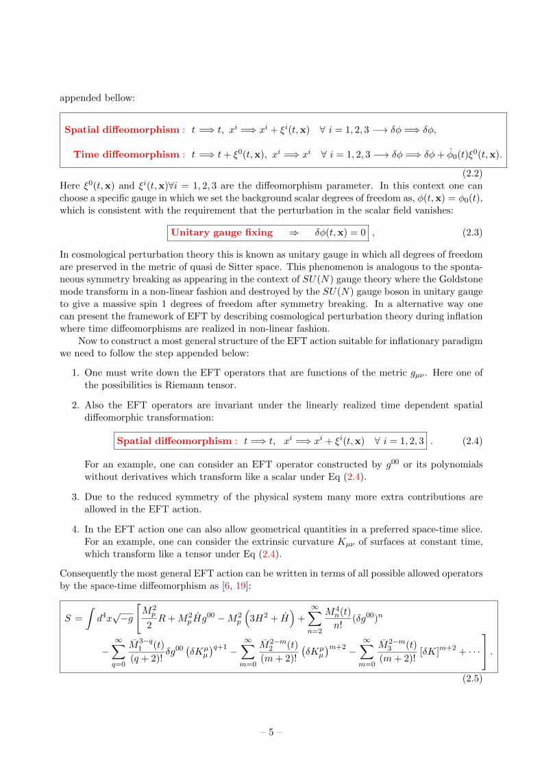
Now to construct a most general structure of the EFT action suitable for inflationary paradigmwe need to follow the step appended below:

1. One must write down the EFT operators that are functions of the metric gµν . Here one ofthe possibilities is Riemann tensor.

2. Also the EFT operators are invariant under the linearly realized time dependent spatialdiffeomorphic transformation:

Spatial diffeomorphism : t =⇒ t, xi =⇒ xi + ξi(t,x) ∀ i = 1, 2, 3 . (2.4)

For an example, one can consider an EFT operator constructed by g00 or its polynomialswithout derivatives which transform like a scalar under Eq (2.4).

3. Due to the reduced symmetry of the physical system many more extra contributions areallowed in the EFT action.

4. In the EFT action one can also allow geometrical quantities in a preferred space-time slice.For an example, one can consider the extrinsic curvature Kµν of surfaces at constant time,which transform like a tensor under Eq (2.4).

Consequently the most general EFT action can be written in terms of all possible allowed operatorsby the space-time diffeomorphism as [6, 19]:

S =

∫d4x√−g

[M2p

2R+M2

p Hg00 −M2

p

(3H2 + H

)+

∞∑n=2

M4n(t)

n!(δg00)n

−∞∑q=0

M3−q1 (t)

(q + 2)!δg00

(δKµ

µ

)q+1 −∞∑m=0

M2−m2 (t)

(m+ 2)!

(δKµ

µ

)m+2 −∞∑m=0

M2−m3 (t)

(m+ 2)![δK]m+2 + · · ·

.(2.5)

– 5 –

where the dots stand for higher order fluctuations in the EFT action which contains operators withmore derivatives in space-time metric. Here we use the following sets of definitions for extrinsiccurvature Kµν , unit normal nµ and induced metric hµν :

Kµν = hσµ∇σnν =δ0µ∂νg

00 + δ0ν∂µg

00

2(−g00)3/2+δ0µδ

0νg

0σ∂σg00

2(−g00)5/2− g0ρ (∂µgρν + ∂νgρµ − ∂ρgµν)

2(−g00)1/2,

hµν = gµν + nµnν , nµ =∂µt√

−gµν∂µt∂νt=

δ0µ√−g00

. (2.6)

Here δKµν represents the variation of the extrinsic curvature of constant time surfaces with respectto the unperturbed background FLRW metric in quasi de Sitter space-time:

δg00 = g00 + 1, δKµν = Kµν − a2Hhµν . (2.7)

Additionally, we have used a shorthand notation [δK] to define the following tensor contractionrule useful to quantify the EFT action [19]:

[δK]m+2 = δKµ1µ2 δK

µ2µ3 δK

µ3µ4 · · · δK

µm+1µm+2

δKµm+2µ1 . (2.8)

Before going to the further details let us first point out the few important characteristics of theEFT action which are appended bellow:

• In the EFT action the operators M2p Hg

00 and M2p

(3H2 + H

)are completely specified by the

Hubble parameter H(t) which is the solution of Friedman’s Eqns in unperturbed background.

• Rest of the contributions in EFT action captures the effect of quantum fluctuations, whichare characterized by the perturbation around the background FLRW solution of all UVcomplete theories of inflation.

• The coefficients of the operators appearing in the EFT action are in general time dependent.

Now as we are interested to compute the two and three point correlation function, we have re-stricted to the following truncated EFT action [6, 19]:

S =

∫d4x√−g

[M2p

2R+M2

p Hg00 −M2

p

(3H2 + H

)+M4

2 (t)

2!

(g00 + 1

)2+M4

3 (t)

3!

(g00 + 1

)3− M3

1 (t)

2

(g00 + 1

)δKµ

µ −M2

2 (t)

2(δKµ

µ )2 − M23 (t)

2δKµ

ν δKνµ

].

(2.9)where we have considered the terms in two derivatives in the metric 2.

2As we are dealing with EFT, in principle one can consider opeators which includes higher derivatives in themetric i.e.

(g00 + 1

)2δK2, δK2δKν

µδKµν , δK3, δKδN2 (here δN = N − 1, where N is the lapse function in ADM

formalism. See ref. [56] for more details.) etc contributions. But since we have considered the terms two derivativein the metric we have truncated the EFT action in the form presencted in Eq. (2.9) and the form of the EFT actionis exactly similar with ref. [6]. In this paper our prime objective is to concentrate only on the leading order treelevel contributions and for this reason we have not considered any subleading suppressed contributions or any othercontributions which are coming from the quantum loop corrections. Additionally, we have also neglected the termlike

(g00 + 1

)2δK in the EFT action as this term is suppressed by the contribution H2ε << 1 in the decoupling

limit and also the higher derivatives of the Goldsotone mode π after implementing the symmetry breaking throughStuckelberg trick.

– 6 –

2.2 EFT as a theory of Goldstone Boson

2.2.1 Stuckelberg trick I: An example from SU(N) gauge theory with massive gaugeboson in flat background

In the unitary gauge the EFT action consist of graviton mode two helicities and scalar mode re-spectively. In this context first we apply a broken time diffeomorphic transformation on Goldstoneboson. As a result SU(N) gauge symmetry [6, 57] is non-linearly realized in the framework ofEFT. This mechanism is commonly known as Stuckelberg trick. Let us mention two crucial rolesof Stuckelberg trick in gauge theory:

1. Using this trick in SU(N) gauge theory [6, 57] one can study the physical implications fromlongitudinal components of a massive gauge boson degrees of freedom.

2. It is expected that in the weak coupling limit the contribution from the mixing terms arevery small and consequently Goldstone modes decouple from the theory.

To give a specific example of Stuckelberg trick we consider SU(N) gauge theory characterizedby a non-abelian gauge field Aaµ in the background of Minkowski flat space-time. In unitary gaugethis theory is described by the following action:

S =

∫d4x

[−1

4Tr(FµνF

µν)− m2

2Tr(AµA

µ)

], (2.10)

where Aµ = AaµTa and F aµν = ∂[µAaν]. Here the label a = 1, 2, · · · , N for SU(N) gauge theory. Also

Ta are the generators of non-abelian gauge group which satisfy the following properties:[T a, T b

]= ifabcTc, Tr(T a) = 0, Tr(T aT b) =

δab

2. (2.11)

Here fabc ∀a, b, c = 1, 2, · · · , N are the structure constants of the non-abelian SU(N) gauge theory.It is important to mention that, in this context the SU(N) gauge transformation on the

non-abelian gauge field can be written as:

Aµ =⇒ Aµ =i

gUDµU

†, with Dµ = ∂µ − igAµ (2.12)

where Dµ is the covariant derivative. Here g is the gauge coupling parameter for SU(N) non-abelian gauge theory. Under this gauge transformation each of the terms in the action stated inEq (2.10) transform as:

Tr(FµνFµν) =⇒ Tr(FµνF

µν ) = Tr(FµνFµν), (2.13)

m2

2Tr(AµA

µ) =⇒ m2

2Tr(AµA

µ ) =m2

2gTr[(DµU

†)(DµU)], (2.14)

where U is the unitary operator in SU(N) non-abelian gauge theory.Consequently after doing SU(N) gauge transformation action can be expressed as:

S =⇒ S = S +

∫d4x

[m2

2Tr(AµA

µ)− m2

2gTr[(DµU

†)(DµU)]

]︸ ︷︷ ︸

Additional part which breaks SU(N) gauge symmetry

.(2.15)

– 7 –

where ︸︷︷︸ term signifies the gauge symmetry breaking contribution in the unitary gauge.

Further it is important to note that the SU(N) gauge symmetry can be restored by definingthe previously mentioned unitary operator in a following fashion:

U = exp [iT aπa(t,x)] , (2.16)

where one can identify the πa ∀ a = 1, 2, · · · , N s with the Goldstone modes, which transform ina linear fashion under the action of the following gauge transformation:

U =⇒ U = exp [iT aπa(t,x)] = Σ(t,x) exp [iT aπa(t,x)] = Σ(t,x)︸ ︷︷ ︸Local operator

U. (2.17)

For the sake of simplicity one can rescale the Goldstone modes by absorbing the mass of the SU(N)gauge field m and the SU(N) gauge coupling parameter g by introducing the following canonicalnormalization as given by:

Canonical normalization : πc =m

gπ . (2.18)

Consequently, the action in terms of canonically normalized field πc can be written after SU(N)gauge transformation as:

S =⇒ S = S +

∫d4x

m2

2Tr(AµA

µ)− 1

2Tr[(∂µπc)(∂

µπc)]︸ ︷︷ ︸Kinetic term of Goldstone

−2g2

mTr(Aµ∂

µπc) +g2

2Tr(AµA

µπ2c ) + igTr(πcAµ∂

µπc)︸ ︷︷ ︸Mixing terms after canonical normalization

.(2.19)

It is important to note the important facts from Eq (2.19) which are appended below:

• The last two terms in Eq (2.19) are the mixing terms between the transverse component ofthe SU(N) gauge field, Goldstone boson and its kinetic term respectively.

• Here one can neglect all such mixing contributions at the energy scale Emix >> m. Conse-quently, two sectors decouple from each other as they are weakly coupled in the energy scaleEmix >> m and the Eq (2.19) takes the following form:

S =⇒ S = S +

∫d4x

[m2

2Tr(AµA

µ)− 1

2Tr[(∂µπc)(∂

µπc)]

]. (2.20)

2.2.2 Stuckelberg trick II: Broken time diffeomorphism in quasi de Sitter background

Here one need to perform a time diffeomorphism with a local parameter ξ0(t,x), which is inter-preted as a Goldstone field π(t,x). These Goldstone modes shifts under the application of timediffeomorphism, as given by:

Time diffeomorphism : t =⇒ t+ ξ0(t,x), xi =⇒ xi ∀ i = 1, 2, 3 −→ π(t,x)→ π(t,x)− ξ0(t,x).

(2.21)

– 8 –

The π is the Goldstone mode which describes the scalar perturbations around the backgroundFLRW metric. The effective action in the unitary gauge can be reproduced by gauge fixing thetime diffeomorphism as:

Unitary gauge fixing ⇒ π(t,x) = 0 ⇒ π(t,x) = −ξ0(t,x) . (2.22)

To construct the EFT action it is important to write down the transformation property of eachoperators under the application of broken time diffeomorphism, which are given by:

1. Rule for metric: Under broken time diffeomorphism contravariant and covariant metrictransform as:

Contravariant metric : g00 =⇒ (1 + π)2g00 + 2(1 + π)g0i∂iπ + gij∂iπ∂jπ,

g0i =⇒ (1 + π)g0i + gij∂jπ,

gij =⇒ gij .

(2.23)

Covariant metric : g00 =⇒ (1 + π)2g00,

g0i =⇒ (1 + π)g0i + g00π∂iπ,

gij =⇒ gij + g0j∂iπ + gi0∂jπ.

(2.24)

2. Rule for Ricci scalar and Ricci tensor: Under broken time diffeomorphism Ricci scalarand the spatial component of the Ricci tensor on 3-hypersurface transform as:

Ricci scalar : (3)R =⇒ (3)R+4

a2H(∂2π),

Spatial Ricci tensor : (3)Rij =⇒ (3)Rij +H(∂i∂jπ + δij∂2π).

(2.25)

3. Rule for extrinsic curvature: Under broken time diffeomorphism trace and the spatial,time and mixed component of the extrinsic curvature transform as:

Trace : δK =⇒ δK − 3πH − 1

a2(∂2π),

Spatial extrinsic curvature : δKij =⇒ δKij − πHhij − ∂i∂jπ

Temporal extrinsic curvature : δK00 =⇒ δK0

0 ,

Mixed extrinsic curvature : δK0i =⇒ δK0

i ,

Mixed extrinsic curvature : δKi0 =⇒ δKi

0 + 2Hgij∂jπ.

(2.26)

– 9 –

4. Rule for time dependent EFT coefficients: Under broken time diffeomorphism timedependent EFT coefficients transform after canonical normalization πc = F 2(t)π as:

EFT coefficient : F (t) =⇒ F (t+ π) =

[ ∞∑n=0

πn

n!

dn

dtn

]F (t)

=

∞∑n=0

πncn!F 2n︸ ︷︷ ︸

Suppression

dn

dtn

F (t) ≈ F (t) .

(2.27)

Here F (t) corresponds to all EFT coefficients mention in the EFT action.

5. Rule for Hubble parameter: Under broken time diffeomorphism, time dependent EFTcoefficients transform after using the following canonical normalization:

Canonical normalization : πc = F 2(t)π , (2.28)

as given by:

Hubble parameter : H(t) =⇒ H(t+ π) =

[ ∞∑n=0

πn

n!

dn

dtn

]H(t)

=

1− πH(t)ε− π2H(t)

2

(ε− 2ε2

)+ · · ·︸ ︷︷ ︸

Correction terms

H(t) .

(2.29)Here ε = −H/H2 is the slow-roll parameter.

Now to construct the EFT action we need to also understand the behaviour of all the operatorsappearing in the weak coupling regime of EFT. In this regime one can neglect the mixing con-tributions between the gravity and Goldstone modes. To demonstrate this explicitly let us startwith the EFT operator:

O1(t) = −HM2p g

00. (2.30)

Under broken time diffeomorphism, the operator O(t) transform as:

O1(t) =⇒[1 +

π

ε

(ε− 2Hε2

)+ · · ·

] [(1 + π)2O1(t)− HM2

p

(2(1 + π)∂iπg

0i + gij∂iπ∂jπ)]

.

(2.31)For further simplification the temporal component of the metric g00 can be written as, g00 =g00 + δg00, where the background metric is given by, g00 = −1 and the metric fluctuation ischaracterized by δg00 [6, 19]. Using this in Eq (2.31) and considering only the first term inEq (2.31) we get a kinetic term, M2

p Hπ2 ¯g00 and a mixing contribution, M2

p Hπδg00 respectively.

Further we use a canonical normalized metric fluctuation from the mixing contribution as givenby:

Canonical normalization : δg00c = Mpδg

00 , (2.32)

in terms of which one can write, M2p Hπδg

00 =√Hπcδg

00c . Consequently, at above the energy

scale Emix =√H, we can neglect this mixing term in the weak coupling regime.

– 10 –

One can also consider mixing contributions M2p Hπ

2δg00 and πM2p Hπg

00, which can be recast

after canonical normalization as, M2p Hπ

2δg00 = π2c δg

00c /Mp and πM2

p Hπg00 = Hπcπcg

00/H with

H/H << 1. Here all higher order terms in π will lead to additional Planck-suppression aftercanonical normalization. Consequently, we can neglect the contribution from M2

p Hπδg00 term at

the scale E > Emix. Finally, in the weak coupling regime one can recast Eq (2.31) as:

O1(t) =⇒ O1(t)

[π2 − 1

a2(∂iπ)2

]. (2.33)

2.2.3 The Goldstone action from EFT

Finally in the weak coupling limit (or decoupling limit) we get the following simplified EFT action:

SEFT = Sg + Sπ, (2.34)

where the gravitational part and the Goldstone action is given by:

Sg =

∫d4x√−g

[M2p

2R−M2

p

(3H2 + H

)], (2.35)

Sπ = S(2)π + S(3)

π + · · · , (2.36)

where the second and third order Goldstone action can be written as:

S(2)π =

∫d4x a3

[−M2

p H

(π2 − 1

a2(∂iπ)2

)+ 2M4

2 π2

+1

2

(M2

3 + 3M22

)H2(1− ε)(∂iπ)2

a2−(M2

3 + 3M22

)H2 (∂iπ)2

a2− M3

1 π1

a2(∂2i π)

].

(2.37)

S(3)π =

∫d4x a3

[(2M4

2 −4

3M4

3

)π3 − 2M4

2 π1

a2(∂iπ)2

− M23πH

1

a2∂2i π − 3M2

2 Hπ1

a2(∂2i π) +

3

2M3

1πH1

a2(∂iπ)2

− 3

2M3

1 Hππ2 − M3

1 π1

a2(∂iπ)2

].

(2.38)

Here we introduce EFT sound speed cS as:

cS ≡1√

1− 2M42

HM2p

. (2.39)

Here if we set M2 = 0 or equivalently if we say thatM4

22! (g00 + 1)2 term is absent in the effective

Lagrangian then Eq (2.39) suggests that in that case sound speed cS = 1, which is true for singlefield canonical slow roll inflation. Next using Eq (2.39) and applying integration by parts in the

– 11 –

Goldstone part of the Lagrangian we get 3:

S(2)π =

∫d4x a3

(−M2p H

c2S

)[π2 − c2

S

(1− M3

1H

M2p H−[M2

3 + 3M22

] H2(1 + ε)

2M2p H

)1

a2(∂iπ)2

]. (2.44)

S(3)π =

∫d4x a3

[(1− 1

c2S

)HM2

p +3

2M3

1H −4

3M4

3

π3

−(

1− 1

c2S

)HM2

p +3

2M3

1H

1

a2π(∂iπ)2

− 9

2M3

1H2ππ2 +

3

2M3

1H1

a2πd

dt(∂iπ)2

].

(2.45)

In the present context metric fluctuation of the spatial components are given by:

gij = a2(t) [(1 + 2ζ(t,x)) δij + γij ] ∀ i = 1, 2, 3, (2.46)

where a(t) is the scale factor in FLRW quasi de Sitter background space-time. Also ζ(t,x) isknown as curvature perturbation which signifies scalar fluctuation. On the other hand, tensorfluctuations are identified with γij , which is spin-2, transverse and traceless rank 2 tensor. Hereunder the broken time diffeomorphism the scale factor a(t) transforms in the following fashion:

a(t) =⇒ a(t− π(t,x)) = a(t)−Hπ(t,x)a(t) + · · · ≈ a(t) (1−Hπ(t,x)) . (2.47)

Further using Eq (2.46) and Eq (2.47), we get:

a2(t) (1−Hπ(t,x))2 ≈ a2(t) (1− 2Hπ(t,x)) = a2(t) (1 + 2ζ(t,x)) . (2.48)

This implies that the curvature perturbation ζ(t,x) can be written in terms of Goldstone modesπ(t,x) in the following way 4:

Quantum fluctuation in terms of Goldstone mode : ζ(t,x) = −Hπ(t,x) . (2.50)

3Let us concentrate on the following contribution in the second and third order peturbed EFT action, which canbe written after integration by parts as:

S2π ⊃ −

∫d3x dt a3 M3

1π

a2(∂2i π)

=

∫d3x dt a3

M31

a2

[−∂i (π∂iπ) +

1

2

d

dt(∂iπ)2

]=

∫d3x dt a3

M31

2

[d

dt

((∂iπ)2

a2

)− H

a2(∂iπ)2

]= −

∫d3x dt a3

M31

2H

(∂iπ)2

a2. (2.40)

S3π ⊃ −

∫d3x dt a3 M3

13

2H π π2 =

∫d3x dt a3

[3

2M3

1Hπ3 − 9

2H2M3

1ππ2

]. (2.41)

S3π ⊃

∫d3x dt a3 M3

13

2H π

(∂iπ)2

a2= −

∫d3x dt a3

[3

2M3

1Hπ

a2(∂iπ)2 +

π

a23

2M3

1 (∂iπ)2]. (2.42)

S3π ⊃ −3

∫d3x dt a3 M2

2 H ππ

a2(∂2i π)

=

∫d3x dt a3 3M2

2

[Hπ

a2(∂iπ)2 +

π

a2(∂iπ)2

]. (2.43)

4Here we have considered the linear relation between the curvature perturbation (ζ) and the Goldstone mode (π).In this context one can consider the following non-linear relation to compute the three point correlation functionfrom the present setup:

ζ(t,x) = −Hπ(t,x)− (ε− η)

2H2π2(t,x) + · · · , (2.49)

– 12 –

Further using Eq (2.50), the effective action for the Goldstone part of the Lagrangian can be recastin terms of curvature perturbation ζ(t,x) as:

S(2)ζ ≈

∫d4x a3

(M2p ε

c2S

)[ζ2 − c2

S

(1− M3

1H

M2p H−[M2

3 + 3M22

] H2(1 + ε)

2M2p H

)1

a2(∂iζ)2

]. (2.51)

S(3)ζ ≈

∫d4x

a3

H3

[−(

1− 1

c2S

)HM2

p +3

2M3

1H −4

3M4

3

ζ3

+

(1− 1

c2S

)HM2

p +3

2M3

1H

1

a2ζ(∂iζ)2

+9

2M3

1H2ζζ2 − 3

2M3

1H1

a2ζd

dt(∂iζ)2

].

(2.52)

For further simplification we introduce few new parameters which are appended bellow 5:

• First of all we define an effective sound speed cS , which can be expressed in terms of theusual EFT sound speed cS as 6:

cS = cS

√1− M3

1H

M2p H−[M2

3 + 3M22

] H2(1 + ε)

2M2p H

. (2.53)

Since the following approximations:∣∣∣∣∣M31H

M2p H

∣∣∣∣∣ << 1,

∣∣∣∣∣[M23 + 3M2

2

] H2(1 + ε)

2M2p H

∣∣∣∣∣ << 1, (2.54)

are valid in the present context of discussion, one can recast the effective sound speed in thefollowing simplified form as:

cS ≈ cS

1 +

1

2εHM2p

[M3

1 +(M2

3 + 3M22

) H(1 + ε)

2

]. (2.55)

where the slow-roll parameters are given by, ε = −H/H2 and η = ε − 12d ln εdN . Here N =

∫H dt, represents the

number of e-foldings. However the contribution from such non-linear term is extremely small and proportional tosubleading terms ε2, η2 and εη in the expression for the three point function and the associated bispectrum. From theobservational perspective such contributions also not so important and can be treated as very very small correctionto the leading order result computed in this paper.

5Here we have used few choices for the simplifications of the further computation of the two and three pointcorrelation function in the EFT coefficients which are partly motivated from the ref. [58]. Also it is important tonote that, since we are restricted our computation up to tree level and and not considering any quantum effectsthrough loop correction, we have discussed the radiative stablity or naturalness of these choices under quantumcorrections.

6Here it is important to point out that, in the case when M2 = 0 we have the EFT sound speed cS = 1 exactly,which is true for all canonical slow-roll models of inflation driven by a single field. But since here the EFT coefficientsare sufficitly small Mi∀i = 1, 2, 3(∼ O(10−2 − 10−3)) it is expected that cS ≈ cS and for the situation cS = 1 onecan approximately fix cS ≈ 1. So for canonical slow-roll model one can easily approimate the redefined soundspeed cS with the ususal EFT sound speed cS without loosing any generality. But such small EFT coefficientsMi∀i = 1, 2, 3(∼ O(10−2 − 10−3)) play significant role in the computation of the three point function and theassociated bispectrum as in the absence of these coefficients the amplitude of the bispectrum fNL is zero. Thisalso implies that for canonical slow-roll model of single field inflation the amount of non-Gaussinity is not verylarge and this completely consistent with the previous finding that in that case the amplitude of the bispectrumfNL ∝ ε (where ε is the slow-roll parameter), at the leading order of the computation. See ref. [30] for details.

– 13 –

• Secondly, we introduce the following connecting relationship between M3 and M2 given by:

M43 c

2S = −c3M

42 . (2.56)

When M2 = 0 then from Eq (2.39) we can see that the sound speed cS = 1 and Eq (2.56)also implies that M3 = 0 in that case.

• Next we define the following connecting relationship between M3 and M1 given by:

M43 c4 = −HM3

1 c3. (2.57)

When M2 = 0 then from Eq (2.39) we can see that the sound speed cS = 1 (which is actuallythe result for single field canonical slow-roll models of inflation) and Eq (2.56) and Eq (2.57)also implies the following possibilities:

1. M3 = 0, M1 6= 0 and c3c4→ 0. We will look into this possibility in detail during our

computation for cS = 1 case as this will finally give rise to non vanishing three pointfunction (non-gaussianity).

2. M3 = 0, M1 = 0 and c3c46= 0. We don’t consider this possibility for cS = 1 case because

for this case third (S(3)ζ ) action for curvature perturbation vanishes, which will give rise

zero three point function (non-gaussianity).

• For further simplification one can also assume that:

M23 + 3M2

2 =M3

1

Hc5(2.58)

so that one can write:

1

εHM2p

[M3

1 +(M2

3 + 3M22

) H(1 + ε)

2

]=

M31

εHM2p

[1 +

(1 + ε)

2c5

]. (2.59)

For cS = 1 this implies the following two possibilities:

1. M1 6= 0 and c5 = −12(1 + ε). We will look into this possibility in detail during our

computation for cS = 1 case as this will finally give rise to non vanishing three pointfunction (non-gaussianity).

2. M1 = 0. We don’t consider this possibility for cS = 1 case because for this case third

(S(3)ζ ) action for curvature perturbation vanishes, which will give rise zero three point

function (non-gaussianity).

Consequently, the effective sound speed can be recast as:

cS = cS

√1 +

∆M31

2εHM2p

≈ cS

1 +∆M3

1

4εHM2p

(2.60)

where ∆ is defined as, ∆ = 2+ 1+εc5. Here ∆ = 0 for c5 = −1

2(1+ε) when cS = 1. Consequentlywe have cS = cS = 1 in that case.

• For further simplification one can also assume that:

M23 ≈ M2

2 =M3

1

4Hc5. (2.61)

Here cS = 1 this implies the following two possibilities:

– 14 –

1. M23 ≈ M2

2 6= 0, M1 6= 0 and c5 = −12(1 + ε) as mentioned earlier. We will look into this

possibility in detail during our computation for cS = 1 case as this will finally give riseto non vanishing non-gaussianity.

2. M23 ≈ M2

2 = 0, M1 = 0. As mentioned earlier here we don’t consider this possibility

for cS = 1 case because for this case second (S(2)ζ ) and third order (S

(3)ζ ) action for

curvature perturbation vanishes, which will give rise zero non-gaussianity.

• Next we define the following connecting relationship between M4 and M3 given by:

M44 c6 = M4

3 c4 = −HM31 c3. (2.62)

When M2 = 0 then from Eq (2.39) we can see that the sound speed cS = 1 and Eq (2.56)and Eq (2.62) also implies the following possibilities:

1. M4 6= 0, M3 = 0, M1 6= 0 and c3c4→ 0. We will look into this possibility in detail during

our computation for cS = 1 case as this will finally give rise to non vanishing threepoint function (non-gaussianity).

2. M4 = 0, M3 = 0, M1 = 0 and c3c46= 0. We don’t consider this possibility for cS = 1

case because for this case third (S(3)ζ ) order action for curvature perturbation vanishes,

which will give rise zero three point function (non-gaussianity).

Further using all such new defined parameters the EFT action for Goldstone boson can be recastas 7:

For cS = 1 :

S(2)ζ ≈

∫d4x a3 M2

p ε

[ζ2 − 1

a2(∂iζ)2

]. (2.63)

S(3)ζ ≈

∫d4x

a3

H3

[−

3

2M3

1H

ζ3 +

3

2M3

1H

1

a2ζ(∂iζ)2

+9

2M3

1H2ζζ2 − 3

2M3

1H1

a2ζd

dt(∂iζ)2

].

(2.64)

For cS < 1 :

S(2)ζ ≈

∫d4x a3

(M2p ε

c2S

)[ζ2 − c2

S

1

a2(∂iζ)2

]. (2.65)

S(3)ζ ≈

∫d4x a3

εM2p

H

(1− 1

c2S

)[1 +

3c4

4c2S

+2c3

3c2S

ζ3 −

1 +

3c4

4c2S

1

a2ζ(∂iζ)2

− 9Hc4

4c2S

ζζ2 +3c4

4c2S

1

a2ζd

dt(∂iζ)2

].

(2.66)

7Here it is important to note that, for the case cS = 1 we have written an approximated form of the second andthird order action by assuming that cS ≈ cS ∼ 1, which is true for all canonical slow-roll models of inflation drivenby a single field. Here the EFT coefficients are sufficitly small Mi∀i = 1, 2, 3(∼ O(10−2 − 10−3)) for which it isexpected that cS ≈ cS and for the situation cS = 1 one can approximately fix cS ≈ 1.

– 15 –

3 Two point correlation function from EFT

3.1 For scalar modes

3.1.1 Mode equation and solution for scalar perturbation

Here we compute the two point correlation from scalar perturbation. For this purpose we considerthe second order perturbed action as given by 8:

S(2)ζ ≈

∫d4x a3

(M2p ε

c2S

)[ζ2 − c2

S

(1− M3

1H

M2p H−[M2

3 + 3M22

] H2(1 + ε)

2M2p H

)1

a2(∂iζ)2

], (3.1)

which can be recast for cS = 1 and cS < 1 case as:

For cS = 1 : S(2)ζ ≈

∫d4x a3 M2

p ε

[ζ2 − 1

a2(∂iζ)2

], (3.2)

For cS < 1 : S(2)ζ ≈

∫d4x a3

(M2p ε

c2S

)[ζ2 − c2

S

1

a2(∂iζ)2

], (3.3)

where the effective sound speed cS is defined earlier.Next we define Mukhanov-Sasaki variable variable v(η,x) which is defined as:

Mukhanov − Sasaki variable : v(η,x) = z ζ(η,x) Mp = −z H π(η,x) Mp . (3.4)

In general the parameter z is defined for the present EFT setup as, z = a√

2εcS

. Now in terms ofv(η,x) the second order action for the curvature perturbation can be recast as:

S(2)ζ ≈

∫d3x dη

[v′2 − c2

S(∂iv)2 1

a2(∂iζ)2 −m2

eff (η)v2

], (3.5)

where the effective mass parametermeff (η) is defined as, m2eff (η) = −1

zd2zdη2

. Here η is the conformal

time which can be expressed in terms of physical time t as, η =∫

dta(t) . The conformal time described

here is negative and lying within −∞ < η < 0. During inflation the scale factor and the parameterz can be expressed in terms of the conformal time η as:

a(η) =

− 1

Hηfor dS

− 1

Hη(1 + ε) for qdS.

(3.6)

and

z =a√

2ε

cS=

− 1

Hη

√2ε

cSfor dS

− 1

Hη

√2ε

cS(1 + ε) for qdS.

(3.7)

Additionally it is important to note that for de Sitter and quasi de Sitter case the relation betweenconformal time η and physical time t can be expressed as, t = − 1

H ln(−Hη). Within this setupinflation ends when the conformal time η ∼ 0.

8See also ref. [30] and [43], where similar computation have performed for canonical single field slow roll andgeneralized slow roll models of inflation in presence of Bunch-Davies vacuum state.

– 16 –

Now further doing the Fourier transform:

v(η,x) =

∫d3k

(2π)3vk(η) eik.x (3.8)

one can write down the equation of motion for scalar fluctuation as:

Mukhanov − Sasaki Eqn for scalar mode : v′′k +

(c2Sk

2 +m2eff (η)

)vk = 0 . (3.9)

Here it is important to note that for de Sitter and quasi de Sitter case the effective mass parametercan be expressed as:

m2eff (η) =

− 2

η2for dS

−(ν2 − 1

4

)η2

for qdS.

(3.10)

Here in the de Sitter and quasi de Sitter case the parameter ν can be written as:

ν =

3

2for dS

3

2+ 3ε− η +

s

2for qdS,

(3.11)

where ε, η and s are the slow-roll parameter defined as:

ε = − H

H2, η = 2ε− ε

2Hε, s =

cSHcS

. (3.12)

In the slow-roll regime of inflation ε << 1 and |η| << 1 and at the end of inflation sow-rollcondition breaks when any of the criteria satisfy, (1) ε = 1 or |η| = 1, (2) ε = 1 = |η|.

The general solution for vk(η) thus can be written as:

vk(η) =

√−η[C1H

(1)32

(−kcSη) + C2H(2)32

(−kcSη)]

for dS

√−η[C1H

(1)ν (−kcSη) + C2H

(2)ν (−kcSη)

]for qdS.

(3.13)

Here C1 and C2 are the arbitrary integration constants and the numerical values depend on thechoice of the initial vacuum. In the present context we consider the following choice of the vacuumfor the computation:

1. Bunch Davies vacuum: In this case we choose, C1 = 1, C2 = 0 .

2. α, β vacuum: In this case we choose C1 = coshα,C2 = eiβ sinhα . Here β is a phase factor.

For the most general solution as stated in Eq (3.13) one can consider the limiting physical situa-tions, as given by, I. Superhorizon regime: kcSη << −1, II. Horizon crossing: kcSη = −1,III. Subhorizon regime: kcSη >> −1.

Finally, considering the behaviour of the mode function in the subhorizon regime and super-horizon regime one can write the expression in de Sitter and quasi de Sitter case as:

vk(η) =

1

iη

1√

2 (kcS)32

[C1e

−ikcSη (1 + ikcSη) e−iπ − C2eikcSη (1− ikcSη) eiπ

]for dS

2ν−32

1

iη

1√

2 (kcS)32

(−kcSη)32−ν

∣∣∣∣∣ Γ(ν)

Γ(32

) ∣∣∣∣∣ [C1e−ikcSη (1 + ikcSη) e−

iπ2 (ν+ 1

2 )

− C2eikcSη (1− ikcSη) e

iπ2 (ν+ 1

2 )]

for qdS.

– 17 –

Further using Eq (3.14) one can write down the expression for the curvature perturbation ζ(η,k) =vk(η)z Mp

as:

ζ(η,k) =

iHcS

2 Mp√ε (kcS)

32

[C1e

−ikcSη (1 + ikcSη) e−iπ − C2eikcSη (1− ikcSη) eiπ

]for dS

2ν−32

iHcS

2 Mp√ε(1 + ε)(cSk)

32

(−kcSη)32−ν

∣∣∣∣∣ Γ(ν)

Γ(32

) ∣∣∣∣∣ [C1e−ikcSη (1 + ikcSη) e−

iπ2 (ν+ 1

2 )

− C2eikcSη (1− ikcSη) e

iπ2 (ν+ 1

2 )]

for qdS.

One can further compute the two point function for scalar fluctuation as:

〈ζ(η,k)ζ(η,q)〉 = (2π)3δ(3)(k + q)Pζ(k, η) , (3.14)

where Pζ(k, η) is the power spectrum at time η for scalar fluctuations and in the present contextit is defined as:

Pζ(k, η) =|vk(η)|2

z2M2p

=

H2

4 M2p εcS

1

k3

∣∣∣C1e−ikcSη (1 + ikcSη) e−iπ − C2e

ikcSη (1− ikcSη) eiπ∣∣∣2 for dS

22ν−3 H2

4 M2p ε(1 + ε)2cS

1

k3(−kcSη)3−2ν

∣∣∣∣∣ Γ(ν)

Γ(32

) ∣∣∣∣∣2

∣∣∣C1e−ikcSη (1 + ikcSη) e−

iπ2 (ν+ 1

2 ) − C2eikcSη (1− ikcSη) e

iπ2 (ν+ 1

2 )∣∣∣2 for qdS.

(3.15)

3.1.2 Primordial power spectrum for scalar perturbation

Finally at the horizon crossing one can write further the two point correlation function as 9:

〈ζ(k)ζ(q)〉 = (2π)3δ(3)(k + q)Pζ(k) , (3.16)

where Pζ(k) is the power spectrum at time η for scalar fluctuations and it is defined as:

Pζ(k) =

[|vk(η)|2

z2M2p

]|kcSη|=1

= Pζ(k∗)1

k3=

H2

4 M2p εcS

1

k3[|C1|2 + |C2|2 − (C∗1C2 + C1C

∗2 )]

for dS

22ν−3 H2

4 M2p ε(1 + ε)2cS

1

k3

∣∣∣∣∣ Γ(ν)

Γ(32

) ∣∣∣∣∣2 [|C1|2 + |C2|2

−(C∗1C2e

iπ(ν+ 12 ) + C1C

∗2 e−iπ(ν+ 1

2 ))]

for qdS,

(3.17)

where Pζ(k∗) is power spectrum for scalar fluctuation at the pivot scale k = k∗.For simplicity onecan keep k3/2π2 dependence outside and further define amplitude of the power spectrum ∆ζ(k∗)at the pivit scale k = k∗ as:

∆ζ(k∗) =k3

2π2Pζ(k) =

1

2π2Pζ(k∗) =

H2

8π2 M2p εcS

[|C1|2 + |C2|2 − (C∗1C2 + C1C

∗2 )]

for dS

22ν−3 H2

8π2 M2p ε(1 + ε)2cS

∣∣∣∣∣ Γ(ν)

Γ(32

) ∣∣∣∣∣2 [|C1|2 + |C2|2

−(C∗1C2e

iπ(ν+ 12 ) + C1C

∗2 e−iπ(ν+ 1

2 ))]

for qdS.

(3.18)

For Bunch Davies and α, β vacua power spectrum can be written as:

9See also ref. [30] and [43], where similar computation have performed for canonical single field slow roll andgeneralized slow roll models of inflation in presence of Bunch-Davies vacuum state.

– 18 –

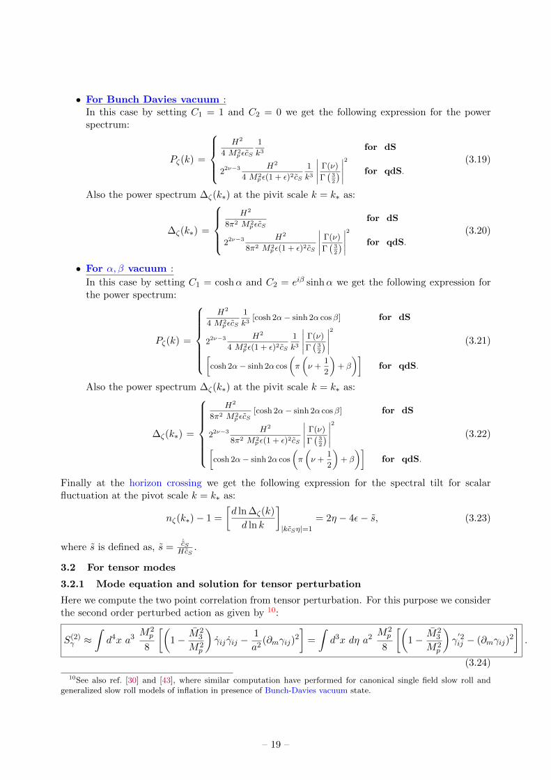
• For Bunch Davies vacuum :In this case by setting C1 = 1 and C2 = 0 we get the following expression for the powerspectrum:

Pζ(k) =

H2

4 M2p εcS

1

k3for dS

22ν−3 H2

4 M2p ε(1 + ε)2cS

1

k3

∣∣∣∣∣ Γ(ν)

Γ(32

) ∣∣∣∣∣2

for qdS.(3.19)

Also the power spectrum ∆ζ(k∗) at the pivit scale k = k∗ as:

∆ζ(k∗) =

H2

8π2 M2p εcS

for dS

22ν−3 H2

8π2 M2p ε(1 + ε)2cS

∣∣∣∣∣ Γ(ν)

Γ(32

) ∣∣∣∣∣2

for qdS.(3.20)

• For α, β vacuum :

In this case by setting C1 = coshα and C2 = eiβ sinhα we get the following expression forthe power spectrum:

Pζ(k) =

H2

4 M2p εcS

1

k3[cosh 2α− sinh 2α cosβ] for dS

22ν−3 H2

4 M2p ε(1 + ε)2cS

1

k3

∣∣∣∣∣ Γ(ν)

Γ(32

) ∣∣∣∣∣2

[cosh 2α− sinh 2α cos

(π

(ν +

1

2

)+ β

)]for qdS.

(3.21)

Also the power spectrum ∆ζ(k∗) at the pivit scale k = k∗ as:

∆ζ(k∗) =

H2

8π2 M2p εcS

[cosh 2α− sinh 2α cosβ] for dS

22ν−3 H2

8π2 M2p ε(1 + ε)2cS

∣∣∣∣∣ Γ(ν)

Γ(32

) ∣∣∣∣∣2

[cosh 2α− sinh 2α cos

(π

(ν +

1

2

)+ β

)]for qdS.

(3.22)

Finally at the horizon crossing we get the following expression for the spectral tilt for scalarfluctuation at the pivot scale k = k∗ as:

nζ(k∗)− 1 =

[d ln ∆ζ(k)

d ln k

]|kcSη|=1

= 2η − 4ε− s, (3.23)

where s is defined as, s =˙cSHcS

.

3.2 For tensor modes

3.2.1 Mode equation and solution for tensor perturbation

Here we compute the two point correlation from tensor perturbation. For this purpose we considerthe second order perturbed action as given by 10:

S(2)γ ≈

∫d4x a3

M2p

8

[(1− M2

3

M2p

)γij γij −

1

a2(∂mγij)

2

]=

∫d3x dη a2

M2p

8

[(1− M2

3

M2p

)γ′2ij − (∂mγij)

2

].

(3.24)

10See also ref. [30] and [43], where similar computation have performed for canonical single field slow roll andgeneralized slow roll models of inflation in presence of Bunch-Davies vacuum state.

– 19 –

In Fourier space one can write γij(η,x) as:

γij(η,x) =∑

λ=×,+

∫d3k

(2π)32

ελij(k) γλ(η,k) eik.x, (3.25)

where the rank-2 polarization tensor ελij satisfies the properties, ελii = kiελij = 0,∑

i,j ελijε

λ′

ij = 2δλλ′ .Similar like scalar fluctuation here we also define a new variable uλ(η,k) in Fourier space as:

uλ(η,k) =a√2Mp γλ(η,k) =

− 1√

2HηMp γλ(η,k) for dS

− 1√2Hη

(1 + ε) Mp γλ(η,k) for qdS.

(3.26)

Using uλ(η,k) one can further write Eq (3.24) as:

S(2)γ ≈

∫d3x dη a2

M2p

4

[(1− M2

3

M2p

)u′2λ (η,k)−

(k2 − a

′′

a

)(uλ(η,k))2

]. (3.27)

From this action one can find out the mode equation for tensor fluctuation as:

Mukhanov − Sasaki Eqn for tensor mode : u′′λ(η,k) +

(k2 − a

′′

a

)(

1− M23

M2p

) uλ(η,k) = 0 . (3.28)

Further we introduce a new parameter cT defined as:

cT =1√

1− M23

M2p

. (3.29)

The general solution for the mode equation for graviton fluctuation can finally written as:

uλ(η,k) =

√−η[D1H

(1)12

√1+8c2

T

(−kcT η) +D2H(2)12

√1+8c2

T

(−kcT η)

]for dS

√−η[D1H

(1)

12

√1+4c2

T (ν2− 14 )

(−kcT η) +D2H(2)

12

√1+4c2

T (ν2− 14 )

(−kcT η)

]for qdS.

(3.30)

Here D1 and D2 are the arbitrary integration constants and the numerical values depend on thechoice of the initial vacuum. In the present context we consider the following choice of the vacuumfor the computation:

1. Bunch Davies vacuum: In this case we choose, D1 = 1, D2 = 0.

2. α, β vacuum: In this case we choose D1 = coshα, D2 = eiβ sinhα. Here β is a phasefactor.

For the most general solution as stated in Eq (3.30) one can consider the limiting physical situa-tions, as given by, I. Superhorizon regime: |kcT η| << 1, II. Horizon crossing: |kcT η| = 1,III. Subhorizon regime: |kcT η| >> 1.

– 20 –

Finally, considering the behaviour of the mode function in the subhorizon regime and super-horizon regime we get:

uλ(η,k) =

212

√1+8c2

T− 3

21

iη

1√

2 (kcT )32

(−kcT η)32− 1

2

√1+8c2

T

∣∣∣∣∣∣Γ(

12

√1 + 8c2T

)Γ(32

)∣∣∣∣∣∣[

D1e−ikcT η (1 + ikcT η) e

− iπ2

(12

√1+8c2

T+ 1

2

)−D2e

ikcT η (1− ikcT η) eiπ2

(12

√1+8c2

T+ 1

2

)]for dS

212

√1+4c2

T (ν2− 14 )− 3

21

iη

1√

2 (kcT )32

(−kcT η)32− 1

2

√1+4c2

T (ν2− 14 )

∣∣∣∣∣∣∣Γ(

12

√1 + 4c2T

(ν2 − 1

4

))Γ(32

)∣∣∣∣∣∣∣[

D1e−ikcT η (1 + ikcT η) e

− iπ2

(12

√1+4c2

T (ν2− 14 )+ 1

2

)−D2e

ikcT η (1− ikcT η) eiπ2

(12

√1+4c2

T (ν2− 14 )+ 1

2

)]for qdS.

(3.31)

Further using Eq (3.14) one can write down the expression for the curvature perturbation ζ(η,k)as:

hλ(η,k) =uλ(η,k)

a Mp=

212

√1+8c2

T− 3

2iH

Mp

1

(kcT )32

(−kcT η)32− 1

2

√1+8c2

T

∣∣∣∣∣∣Γ(

12

√1 + 8c2T

)Γ(32

)∣∣∣∣∣∣[

D1e−ikcT η (1 + ikcT η) e

− iπ2

(12

√1+8c2

T+ 1

2

)−D2e

ikcT η (1− ikcT η) eiπ2

(12

√1+8c2

T+ 1

2

)]for dS

212

√1+4c2

T (ν2− 14 )− 3

2iH

Mp (1 + ε)

1

(kcT )32

(−kcT η)32− 1

2

√1+4c2

T (ν2− 14 )∣∣∣∣∣∣∣

Γ(

12

√1 + 4c2T

(ν2 − 1

4

))Γ(32

)∣∣∣∣∣∣∣[D1e

−ikcT η (1 + ikcT η) e− iπ

2

(12

√1+4c2

T (ν2− 14 )+ 1

2

)

−D2eikcT η (1− ikcT η) e

iπ2

(12

√1+4c2

T (ν2− 14 )+ 1

2

)]for qdS.

(3.32)

3.2.2 Primordial power spectrum for tensor perturbation

One can further compute the two point function for tensor fluctuation as:

〈h(η,k)h(η,q)〉 =∑λ,λ′

〈hλ(η,k)hλ′ (η,q)〉 = (2π)3δ(3)(k + q)Ph(k, η) , (3.33)

where Ph(k, η) is the power spectrum at time η for tensor fluctuations and in the present contextit is defined as:

Ph(k, η) =4|hλ(η,k)|2

a2M2p

=

2√

1+8c2T−3 4H2

M2p

1

(kcT )3(−kcT η)3−

√1+8c2

T

∣∣∣∣∣∣Γ(

12

√1 + 8c2T

)Γ(32

)∣∣∣∣∣∣2

∣∣∣∣D1e−ikcT η (1 + ikcT η) e

− iπ2

(12

√1+8c2

T+ 1

2

)−D2e

ikcT η (1− ikcT η) eiπ2

(12

√1+8c2

T+ 1

2

)∣∣∣∣2 for dS

2

√1+4c2

T (ν2− 14 )−3 4H2

M2p (1 + ε)2

1

(kcT )3(−kcT η)

3−√

1+4c2T (ν2− 1

4 )∣∣∣∣∣∣∣Γ(

12

√1 + 4c2T

(ν2 − 1

4

))Γ(32

)∣∣∣∣∣∣∣2 ∣∣∣∣∣D1e

−ikcT η (1 + ikcT η) e− iπ

2

(12

√1+4c2

T (ν2− 14 )+ 1

2

)

−D2eikcT η (1− ikcT η) e

iπ2

(12

√1+4c2

T (ν2− 14 )+ 1

2

)∣∣∣∣∣2

for qdS.

(3.34)

– 21 –

Finally at the horizon crossing we get the following two point correlation function for tensorperturbation as:

〈h(k)h(q)〉 = (2π)3δ(3)(k + q)Ph(k) , (3.35)

where Ph(k) is known as the power spectrum at the horizon crossing for tensor fluctuations andin the present context it is defined as:

Ph(k) = Ph(k∗)1

k3=

2√

1+8c2T−3 4H2

M2p c

3T

1

k3

∣∣∣∣∣∣Γ(

12

√1 + 8c2T

)Γ(32

)∣∣∣∣∣∣2 [|D1|2 + |D2|2

−(D∗1D2e

iπ(

12

√1+8c2

T+ 1

2

)+D1D

∗2e−iπ

(12

√1+8c2

T+ 1

2

))]for dS

2

√1+4c2

T (ν2− 14 )−3 4H2

M2p (1 + ε)2 c3T

1

k3

∣∣∣∣∣∣∣Γ(

12

√1 + 4c2T

(ν2 − 1

4

))Γ(32

)∣∣∣∣∣∣∣2 [|D1|2 + |D2|2

−

(D∗1D2e

iπ

(12

√1+4c2

T (ν2− 14 )+ 1

2

)+D1D

∗2e−iπ

(12

√1+4c2

T (ν2− 14 )+ 1

2

))]for qdS.

(3.36)

where Ph(k∗) is power spectrum for tensor fluctuation at the pivot scale k = k∗. For simplicity onecan keep k3/2π2 dependence outside and further define amplitude of the power spectrum ∆h(k∗)at the pivit scale k = k∗ as:

∆h(k∗) =k3

2π2Ph(k) =

1

2π2Ph(k∗)

=

2√

1+8c2T−3 2H2

π2M2p c

3T

∣∣∣∣∣∣Γ(

12

√1 + 8c2T

)Γ(32

)∣∣∣∣∣∣2 [|D1|2 + |D2|2

−(C∗1C2e

iπ(

12

√1+8c2

T+ 1

2

)+D1D

∗2e−iπ

(12

√1+8c2

T+ 1

2

))]for dS

2

√1+4c2

T (ν2− 14 )−3 2H2

π2M2p (1 + ε)2 c3T

∣∣∣∣∣∣∣Γ(

12

√1 + 4c2T

(ν2 − 1

4

))Γ(32

)∣∣∣∣∣∣∣2 [|D1|2 + |D2|2

−

(D∗1D2e

iπ

(12

√1+4c2

T (ν2− 14 )+ 1

2

)+D1D

∗2e−iπ

(12

√1+4c2

T (ν2− 14 )+ 1

2

))]for qdS.

(3.37)

For Bunch Davies and α, β vacua we get:

• For Bunch Davies vacuum :In this case by setting D1 = 1 and D2 = 0 we get the following expression for the powerspectrum:

Ph(k) =

2√

1+8c2T−3 4H2

M2p c

3T

1

k3

∣∣∣∣∣∣Γ(

12

√1 + 8c2T

)Γ(32

)∣∣∣∣∣∣2

for dS

2

√1+4c2

T (ν2− 14 )−3 4H2

M2p (1 + ε)2 c3T

1

k3

∣∣∣∣∣∣∣Γ(

12

√1 + 4c2T

(ν2 − 1

4

))Γ(32

)∣∣∣∣∣∣∣2

for qdS.

(3.38)

Also the power spectrum ∆ζ(k∗) at the pivit scale k = k∗ as:

∆h(k∗) =

2√

1+8c2T−3 2H2

π2M2p c

3T

∣∣∣∣∣∣Γ(

12

√1 + 8c2T

)Γ(32

)∣∣∣∣∣∣2

for dS

2

√1+4c2

T (ν2− 14 )−3 2H2

π2M2p (1 + ε)2 c3T

∣∣∣∣∣∣∣Γ(

12

√1 + 4c2T

(ν2 − 1

4

))Γ(32

)∣∣∣∣∣∣∣2

for qdS.

(3.39)

– 22 –

• For α, β vacuum :

In this case by setting D1 = coshα and D2 = eiβ sinhα we get the following expression forthe power spectrum:

Ph(k) =

2√

1+8c2T−3 4H2

M2p c

3T

1

k3

∣∣∣∣∣∣Γ(

12

√1 + 8c2T

)Γ(32

)∣∣∣∣∣∣2

[cosh 2α− sinh 2α cos

(π

(1

2

√1 + 8c2T +

1

2

)+ β

)]for dS

2

√1+4c2

T (ν2− 14 )−3 4H2

M2p (1 + ε)2 c3T

1

k3

∣∣∣∣∣∣∣Γ(

12

√1 + 4c2T

(ν2 − 1

4

))Γ(32

)∣∣∣∣∣∣∣2

[cosh 2α− sinh 2α cos

(π

(1

2

√1 + 4c2T

(ν2 − 1

4

)+

1

2

)+ β

)]for qdS.

(3.40)

Also the power spectrum ∆ζ(k∗) at the pivit scale k = k∗ as:

∆h(k∗) =

2√

1+8c2T−3 2H2

π2M2p c

3T

∣∣∣∣∣∣Γ(

12

√1 + 8c2T

)Γ(32

)∣∣∣∣∣∣2

[cosh 2α− sinh 2α cos

(π

(1

2

√1 + 8c2T +

1

2

)+ β

)]for dS

2

√1+4c2

T (ν2− 14 )−3 2H2

π2M2p (1 + ε)2 c3T

∣∣∣∣∣∣∣Γ(

12

√1 + 4c2T

(ν2 − 1

4

))Γ(32

)∣∣∣∣∣∣∣2

[cosh 2α− sinh 2α cos

(π

(1

2

√1 + 4c2T

(ν2 − 1

4

)+

1

2

)+ β

)]for qdS.

(3.41)

Now let us consider a special case for tensor fluctuation where cT = 1 and it implies the followingtwo possibilities:

1. M3 = 0. But for this case as we have assumed earlier M23 ≈ M2

3 = M31 /4Hc5, then M1 = 0

which is not our matter of interest in this work as this leads to zero three point function forscalar fluctuation. But if we assume that M2

3 6= M23 but M2

3 = M31 /4Hc5 then by setting

M3 = 0 one can get M1 6= 0, which is necessarily required for non-vanishing three pointfunction for scalar fluctuation.

2. M3 << Mp. In this case if we assume M23 ≈ M2

3 = M31 /4Hc5, then M3

1 /4Hc5M2p << 1 and

M2 << Mp. This is perfectly ok of generating non-vanishing three point function for scalarfluctuation.

If we set cT = 1 then for Bunch Davies and α, β vacua power spectrum can be recast into thefollowing simplified form:

• For Bunch Davies vacuum :In this case by setting D1 = 1 and D2 = 0 we get the following expression for the powerspectrum:

Ph(k) =

4H2

M2p

1

k3for dS

22ν−3 4H2

M2p (1 + ε)2

1

k3

∣∣∣∣∣ Γ (ν)

Γ(32

) ∣∣∣∣∣2

for qdS.(3.42)

– 23 –

Also the power spectrum ∆ζ(k∗) at the pivit scale k = k∗ as:

∆h(k∗) =

2H2

π2M2p

for dS

2ν−3 2H2

π2M2p (1 + ε)2

∣∣∣∣∣ Γ (ν)

Γ(32

) ∣∣∣∣∣2

for qdS.(3.43)

• For α, β vacuum :

In this case by setting D1 = coshα and D2 = eiβ sinhα we get the following expression forthe power spectrum:

Ph(k) =

4H2

M2p

1

k3[cosh 2α− sinh 2α cosβ] for dS

22ν−3 4H2

M2p (1 + ε)2

1

k3

∣∣∣∣∣ Γ (ν)

Γ(32

) ∣∣∣∣∣2 [

cosh 2α− sinh 2α cos

(π

(ν +

1

2

)+ β

)]for qdS.

(3.44)

Also the power spectrum ∆ζ(k∗) at the pivit scale k = k∗ as:

∆h(k∗) =

2H2

π2M2p

[cosh 2α− sinh 2α cosβ] for dS

22ν−3 2H2

π2M2p (1 + ε)2

∣∣∣∣∣ Γ (ν)

Γ(32

) ∣∣∣∣∣2

[cosh 2α− sinh 2α cos

(π

(ν +

1

2

)+ β

)]for qdS.

(3.45)

4 Scalar Three point correlation function from EFT

4.1 Basic setup

Here we compute the three point correlation function for perturbations from scalar modes. Forthis purpose we consider the third order perturbed action for the scalar modes as given by 11:

S(3)ζ ≈

∫d4x

a3

H3

[−(

1− 1

c2S

)HM2

p+3

2M3

1H −4

3M4

3

ζ3

+

(1− 1

c2S

)HM2

p+3

2M3

1H

1

a2ζ(∂iζ)2

+9

2M3

1H2ζζ2−3

2M3

1H1

a2ζd

dt(∂iζ)2

],

(4.1)

11Here it is important to note that the red colored terms are the new contribution in the EFT action consideredin this paper, which are not present in ref. [6]. From the EFT action itself it is clear that for effective sound speedcS = 1 three point correlation function and the associated bispectrum vanishes if we don’t contribution these redcolored terms. This is obviously true if we fix cS = 1 in the result obtained in ref. [6]. On the other hand if weconsider these red colored terms then the result is consistent with ref. [30] with cS = 1 and with ref. [43] with cS 6= 1.This implies that cS = 1 is not fully radiatively stable in single field slow roll inflation. However, if we include theeffects produced by quantum correction through loop effects, then a small deviation in the effective sound speed1− cS ∼ ε (H/Mp)

2 can be produced. See ref. [6] where this fact is clearly pointed. But for inflation we know thatin the inflationary regime the slow roll parameter ε < 1 and the scale of inflation is H/Mp << 1, which imply thisdeviation is also very small and not very interesting for our purpose studied in this paper.

– 24 –

which can be recast for cS = 1 and cS < 1 case as:

For cS = 1 :

S(3)ζ ≈

∫d4x

a3

H3

[−

3

2M3

1H

ζ3 +

3

2M3

1H

1

a2ζ(∂iζ)2

+9

2M3

1H2ζζ2−3

2M3

1H1

a2ζd

dt(∂iζ)2

],

(4.2)

For cS < 1 :

S(3)ζ ≈

∫d4x a3

εM2p

H

(1− 1

c2S

)[1 +

3c4

4c2S

+2c3

3c2S

ζ3 −

1+

3c4

4c2S

1

a2ζ(∂iζ)2

−9Hc4

4c2S

ζζ2+3c4

4c2S

1

a2ζd

dt(∂iζ)2

],

(4.3)

To extract further informations from third order action, first of all one needs to start with theFourier transform of the curvature perturbation ζ(η,x) defined as:

ζ(η,x) =

∫d3k

(2π)3ζk(η) exp(ik.x), (4.4)

where ζk(η) is the time dependent part of the curvature fluctuation after Fourier transform andcan be expressed in terms of the normalized time dependent scalar mode function vk(η) as:

ζ(η,k) =vk(η)

zMp=ζ (η,k) a (k) + ζ∗ (η,−k) a† (−k)

zMp(4.5)

where z is explicitly defined earlier and a(k), a†(k) are the creation and annihilation operatorsatisfies the following commutation relations:[

a(k), a†(−k′)]

= (2π)3δ3(k + k′),

[a(k), a(k

′)]

= 0,[a†(k), a†(k

′)]

= 0. (4.6)

4.2 Computation of scalar three point function in interaction picture

Presently our prime objective is to compute the three point function of the curvature fluctuation inmomentum space from S2

ζ with respect to the arbitrary choice of vacuum, which leads to importantresult in the context of primordial cosmology. Further using the interaction picture the three pointfunction of the curvature fluctuation in momentum space can be expressed as:

〈ζ(k1)ζ(k2)ζ(k3)〉 = −i

ηf=0∫ηi=−∞

dη a(η) 〈0|[ζ(ηf ,k1)ζ(ηf ,k2)ζ(ηf ,k3), Hint (η)

]|0〉 , (4.7)

where a(η) is the scale factor defined in the earlier section in terms of Hubble parameter H andconformal time scale η. Here |0〉 represents any arbitrary vacuum state and for discussion we will

– 25 –

only derive the results for Bunch-Davies vacuum and α, β vacuum. In the interaction picture theHamiltonian can written as 12:

Hint(η) = − 1

H3

[−(

1− 1

c2S

)HM2

p +3

2M3

1H −4

3M4

3

ζ3

+

(1− 1

c2S

)HM2

p +3

2M3

1H

1

a2ζ(∂iζ)2

+9

2M3

1H2ζζ2 − 3

2M3

1H1

a2ζd

dt(∂iζ)2

].

(4.8)

which gives the primary information to compute the explicit expression for the three point functionin the present context. After substituting the interaction Hamiltonian we finally get the followingexpression for the three point function for the scalar fluctuation:

〈ζ(k1)ζ(k2)ζ(k3)〉 = −i

ηf=0∫ηi=−∞

dη a(η)

∫d3x

H3

∫ ∫ ∫d3k4

(2π)3

d3k5

(2π)3

d3k6

(2π)3ei(k4+k5+k6).x

α1〈0|

[ζ(ηf ,k1)ζ(ηf ,k2)ζ(ηf ,k3), ζ

′(η,k4)ζ

′(η,k5)ζ

′(η,k6)

]|0〉

− α2(k5.k6)〈0|[ζ(ηf ,k1)ζ(ηf ,k2)ζ(ηf ,k3), ζ

′(η,k4)ζ(η,k5)ζ(η,k6)

]|0〉

+ α3 a(η) 〈0|[ζ(ηf ,k1)ζ(ηf ,k2)ζ(ηf ,k3), ζ(η,k4)ζ

′(η,k5)ζ

′(η,k6)

]|0〉

− α4(k5.k6)〈0|[ζ(ηf ,k1)ζ(ηf ,k2)ζ(ηf ,k3), ζ(η,k4)ζ

′(η,k5)ζ(η,k6)

]|0〉

− α5(k5.k6)〈0|[ζ(ηf ,k1)ζ(ηf ,k2)ζ(ηf ,k3), ζ(η,k4)ζ(η,k5)ζ

′(η,k6)

]|0〉, (4.9)

where the coefficients αj∀j = 1, 2, 3, 4, 5 are defined as 13:

α1 =

(1− 1

c2S

)HM2

p +3

2M3

1H −4

3M4

3

, (4.10)

α2 = −(

1− 1

c2S

)HM2

p +3

2M3

1H

, (4.11)

α3 = −9

2M3

1H2, (4.12)

α4 =3

2M3

1H, (4.13)

α5 =3

2M3

1H. (4.14)

Now let us evaluate the co-efficients of α1, α2, α3, α4 in the present context using Wick’s theorem:

12See also ref. [30] and [43], where similar computation have performed for canonical single field slow roll andgeneralized slow roll models of inflation in presence of Bunch-Davies vacuum state.

13Here it is clearly observed that for canonical single field slow-roll model, which is described by cS = 1 we haveM3 = 0 and other EFT coeffecients are sufficiently small, Mi∀i = 1, 2, 3(∼ O()10−3 − 10−2). This directly impliesthat the contribution in the three point function and in the associated bispectrum is very small and also consistentwith the previous result as obtained in ref. [30]. Additionally it is important to mention that, in momentum spacethe bispectrum containts additional terms in presence of any arbitrary choice of the quantum vacuum initial state.Also, if we compare with the ref. [6]

– 26 –

1. Coefficient of α1:

〈0|[ζ(ηf ,k1)ζ(ηf ,k2)ζ(ηf ,k3), ζ

′(η,k4)ζ

′(η,k5)ζ

′(η,k6)

]|0〉

= 〈0|a(k1)a(k2)a(k3)a†(−k4)a†(−k5)a†(−k6)|0〉v(ηf ,k1)v(ηf ,k2)v(ηf ,k3)v

′∗(ηf ,−k4)v′∗(ηf ,−k5)v

′∗(ηf ,−k6) (4.15)

+〈0|a(k4)a(k5)a(k6)a†(−k1)a†(−k2)a†(−k3)|0〉v∗(ηf ,−k1)v∗(ηf ,−k2)v∗(ηf ,−k3)v

′(η,k4)v

′(η,k5)v

′(η,k6).

2. Coefficient of α2:

(k5.k6)〈0|[ζ(ηf ,k1)ζ(ηf ,k2)ζ(ηf ,k3), ζ

′(η,k4)ζ(η,k5)ζ(η,k6)

]|0〉

= (k5.k6)〈0|a(k1)a(k2)a(k3)a†(−k4)a†(−k5)a†(−k6)|0〉v(ηf ,k1)v(ηf ,k2)v(ηf ,k3)v

′∗(ηf ,−k4)v∗(ηf ,−k5)v∗(ηf ,−k6) (4.16)

+(k5.k6)〈0|a(k4)a(k5)a(k6)a†(−k1)a†(−k2)a†(−k3)|0〉v∗(ηf ,−k1)v∗(ηf ,−k2)v∗(ηf ,−k3)v

′(ηf ,k4)v(ηf ,k5)v(ηf ,k6).

3. Coefficient of α3:

〈0|[ζ(ηf ,k1)ζ(ηf ,k2)ζ(ηf ,k3), ζ(η,k4)ζ

′(η,k5)ζ

′(η,k6)

]|0〉

= 〈0|a(k1)a(k2)a(k3)a†(−k4)a†(−k5)a†(−k6)|0〉v(ηf ,k1)v(ηf ,k2)v(ηf ,k3)v∗(ηf ,−k4)v

′∗(ηf ,−k5)v′∗(ηf ,−k6) (4.17)

+〈0|a(k4)a(k5)a(k6)a†(−k1)a†(−k2)a†(−k3)|0〉v∗(ηf ,−k1)v∗(ηf ,−k2)v∗(ηf ,−k3)v(ηf ,k4)v

′(ηf ,k5)v

′(ηf ,k6).

4. Coefficient of α4:

(k5.k6)〈0|[ζ(ηf ,k1)ζ(ηf ,k2)ζ(ηf ,k3), ζ(η,k4)ζ

′(η,k5)ζ(η,k6)

]|0〉

= (k5.k6)〈0|a(k1)a(k2)a(k3)a†(−k4)a†(−k5)a†(−k6)|0〉v(ηf ,k1)v(ηf ,k2)v(ηf ,k3)v∗(ηf ,−k4)v

′∗(ηf ,−k5)v∗(ηf ,−k6) (4.18)

+(k5.k6)〈0|a(k4)a(k5)a(k6)a†(−k1)a†(−k2)a†(−k3)|0〉v∗(ηf ,−k1)v∗(ηf ,−k2)v∗(ηf ,−k3)v(ηf ,k4)v

′(ηf ,k5)v(ηf ,k6).

5. Coefficient of α5:

(k5.k6)〈0|[ζ(ηf ,k1)ζ(ηf ,k2)ζ(ηf ,k3), ζ(η,k4)ζ(η,k5)ζ

′(η,k6)

]|0〉

= 〈0|a(k1)a(k2)a(k3)a†(−k4)a†(−k5)a†(−k6)|0〉v(ηf ,k1)v(ηf ,k2)v(ηf ,k3)v∗(ηf ,−k4)v∗(ηf ,−k5)v

′∗(ηf ,−k6) (4.19)

+〈0|a(k4)a(k5)a(k6)a†(−k1)a†(−k2)a†(−k3)|0〉v∗(ηf ,−k1)v∗(ηf ,−k2)v∗(ηf ,−k3)v(ηf ,k4)v(ηf ,k5)v

′(ηf ,k6).

– 27 –

where we define v as:

v(η,k) =v(η,k)

zMp. (4.20)

Further we also use the following result to simplify the the co-efficients of α1, α2, α3, α4:

〈0|a(k1)a(k2)a(k3)a†(−k4)a†(−k5)a†(−k6)|0〉= 〈0|a(k4)a(k5)a(k6)a†(−k1)a†(−k2)a†(−k3)|0〉

= (2π)9δ(3)(k4 + k1)

[δ(3)(k5 + k2)δ(3)(k6 + k3) + δ(3)(k5 + k3)δ(3)(k6 + k2)

]+δ(3)(k4 + k2)

[δ(3)(k5 + k1)δ(3)(k6 + k3) + δ(3)(k5 + k3)δ(3)(k6 + k1)

]+δ(3)(k4 + k3)

[δ(3)(k5 + k1)δ(3)(k6 + k3) + δ(3)(k5 + k2)δ(3)(k6 + k1)

]. (4.21)

Finally one can write the following expresion for the three point function for the scalar fluctua-tion 14:

〈ζ(k1)ζ(k2)ζ(k3)〉 = (2π)3δ(3)(k1 + k2 + k3)BEFT (k1, k2, k3) . (4.22)

where BEFT (k1, k2, k3) is the bispectrum for scalar fluctuation. In the present computation onecan further write down the expression for the bispectrum as:

BEFT (k1, k2, k3) =

5∑j=1

αjΘj(k1, k2, k3) , (4.23)

where Θj(k1, k2, k3)∀j = 1, 2, 3, 4, 5 is defined in the next subsections. Here it is important to notethat we have derived the expression for the three point function and the associated bispectrum foreffective sound speed cS = 1 and cS < 1 with a choice of general quantum vacuum state.

4.2.1 Coefficient of α1

Here we can write the function Θ1(k1, k2, k3) as:

Θ1(k1, k2, k3) = 6i

∫ ηf=0

ηi=−∞dη

a(η)

H3

[v(ηf ,k1)v(ηf ,k2)v(ηf ,k3)v

′∗(η,k1)v′∗(η,k2)v

′∗(η,k3)

+ v∗(ηf ,k1)v∗(ηf ,k2)v∗(ηf ,k3)v′(η,−k1)v

′(η,−k2)v

′(η,−k3)

]. (4.24)

14See also ref. [30] and [43], where similar computation have performed for canonical single field slow roll andgeneralized slow roll models of inflation in presence of Bunch-Davies vacuum state.

– 28 –

Further using the integrals from the Appendix we finally get the following simplified expressionfor the three point function for the scalar fluctuations 15:

Θ1(k1, k2, k3) =3H2

16ε3M6p

1

k1k2k3

[1

K3

[(C1 − C2)3 (C∗31 + C∗32

)+ (C∗1 − C∗2 )3 (C3

1 + C32

)]+[(C1 − C2)3C∗1C

∗2 (C∗1 − C∗2 ) + (C∗1 − C∗2 )3C1C2 (C1 − C2)

] 3∑i=1

1

(2ki −K)3

],

(4.26)Finally for Bunch Davies and α, β vacuum we get the following contribution in the three pointfunction for scalar fluctuations:

• For Bunch Davies vacuum:After setting C1 = 1 and C2 = 0 we get:

Θ1(k1, k2, k3) =6H2

16ε3M6p

1

k1k2k3

1

K3, (4.27)

• For α, β vacuum:

After setting C1 = coshα and C2 = eiβ sinhα we get:

Θ1(k1, k2, k3) =3H2

16ε3M6p

1

k1k2k3

1

K3

[(coshα− eiβ sinhα

)3 (cosh3 α+ e−3iβ sinh3 α

)+(

coshα− e−iβ sinhα)3 (

cosh3 α+ e3iβ sinh3 α)]

+1

2

[(coshα− eiβ sinhα

)3e−iβ sinh 2α

(coshα− e−iβ sinhα

)+(

coshα− e−iβ sinhα)3eiβ sinh 2α

(coshα− eiβ sinhα

)] 3∑i=1

1

(2ki −K)3

.

(4.28)

15Here ot is important to point out that in de-Sitter space if we consider the Bunch Davies vacuum state then hereonly the term with 1/K3 will appear explicitly in the expression for the three point function and in the associatedbispectrum. On the other hand if we consider all other non-trivial quantum vacuum state in our computation thenthe rest of the contribution will explicitly appear. From the perspective of observation this is obviously an importantinformation as for the non trivial quantum vacuum state we get additional contribution in the bispectrum whichmay enhance the amplitude of the non-Gaussianity in squeezed limiting configuration. Additionally, it is importantto mention that in quasi de Sitter case we get extra contributions 1/c6ν−9

S and 1/(1+ ε)5. Also the factor 1/(k1k2k3)will be replaced by 1/(k1k2k3)2(ν−1). Consequently, in quasi de Sitter case this contribution in the bispectrum canbe recast as:

Θ1(k1, k2, k3) =3H2

16ε3M6p c

6ν−9S (1 + ε)5

1

(k1k2k3)2(ν−1)

[1

K3

[(C1 − C2)3

(C∗31 + C∗32

)+ (C∗1 − C∗2 )

3 (C3

1 + C32

)]+[(C1 − C2)3 C∗1C

∗2 (C∗1 − C∗2 ) + (C∗1 − C∗2 )3 C1C2 (C1 − C2)

] 3∑i=1

1

(2ki −K)3

],

(4.25)

– 29 –

4.2.2 Coefficient of α2

Here we can write the function Θ2(k1, k2, k3) as:

Θ2(k1, k2, k3) = i

∫ ηf=0

ηi=−∞dη

a(η)

H3

2(k2.k3)

[v(ηf ,k1)v(ηf ,k2)v(ηf ,k3)v

′∗(η,k1)v∗(η,k2)v∗(η,k3)

+ v∗(ηf ,−k1)v∗(ηf ,−k2)v∗(ηf ,−k3)v′(η,−k1)v(η,−k2)v(η,−k3)

]+ 2(k3.k1)

[v(ηf ,k1)v(ηf ,k2)v(ηf ,k3)v

′∗(η,k2)v∗(η,k1)v∗(η,k3)

+ v∗(ηf ,−k1)v∗(ηf ,−k2)v∗(ηf ,−k3)v′(η,−k2)v(η,−k1)v(η,−k3)

]+ 2(k1.k2)

[v(ηf ,k1)v(ηf ,k2)v(ηf ,k3)v

′∗(η,k3)v∗(η,k1)v∗(η,k2)

+ v∗(ηf ,−k1)v∗(ηf ,−k2)v∗(ηf ,−k3)v′(η,−k3)v(η,−k1)v(η,−k2)

].

(4.29)

Using the results derived in Appendix we finally get the following simplified expression for thethree point function for the scalar fluctuations 16:

Θ2(k1, k2, k3) =H2

32ε3M6p c

2S

1

(k1k2k3)3

[k2

1(k2.k3)G1(k1, k2, k3)

+ k22(k1.k3)G2(k1, k2, k3) + k2

3(k1.k2)G3(k1, k2, k3)],

(4.31)

16Here ot is important to point out that in de-Sitter space if we consider the Bunch Davies vacuum state then hereonly the term with 1/K3 will appear explicitly in the expression for the three point function and in the associatedbispectrum. On the other hand if we consider all other non-trivial quantum vacuum state in our computation thenthe rest of the contribution will explicitly appear. From the perspective of observation this is obviously an importantinformation as for the non trivial quantum vacuum state we get additional contribution in the bispectrum whichmay enhance the amplitude of the non-Gaussianity in squeezed limiting configuration. Additionally, it is importantto mention that in quasi de Sitter case we get extra contributions 1/c6ν−7

S and 1/(1+ε)5. Also the factor 1/(k1k2k3)3

will be replaced by 1/(k1k2k3)2ν . Consequently, in quasi de Sitter case this contribution in the bispectrum can berecast as:

Θ2(k1, k2, k3) =H2

32ε3M6p c

6ν−7S (1 + ε)5

1

(k1k2k3)2ν[k21(k2.k3)G1(k1, k2, k3)

+ k22(k1.k3)G2(k1, k2, k3) + k23(k1.k2)G3(k1, k2, k3)],

(4.30)

– 30 –

where the momentum dependent functions G1(k1, k2, k3), G2(k1, k2, k3) and G3(k1, k2, k3) are de-fined as:

G1(k1, k2, k3) =1

K3

[K2 + 2k2k3 +K(K − k1)

] [(C1 − C2)3(C∗31 + C∗32 ) + (C1 − C2)3(C∗31 + C∗32 )

]+

1

(2k1 −K)3

[K2 + 2k2k3 +K(K − 5k1)− 2(K − k1)k1 + 4k2

1

]+

1

(2k2 −K)3

[K2 − 4k2k3 +K(k3 − 5k2) + 6k2

2

]+

1

(2k1 −K)3

[K2 − 4k2k3 +K(k2 − 5k3) + 6k2

3

][(C1 − C2)3C∗1C

∗2 (C∗1 + C∗2 ) + (C∗1 − C∗2 )3C1C2(C1 + C2)

]. (4.32)

G2(k1, k2, k3) =1

K3

[K2 + 2k1k3 +K(K − k2)

] [(C1 − C2)3(C∗31 + C∗32 ) + (C1 − C2)3(C∗31 + C∗32 )

]+

1

(2k2 −K)3

[K2 + 2k1k3 +K(K − 5k2)− 2(K − k2)k2 + 4k2

2

]+

1

(2k1 −K)3

[K2 − 4k1k3 +K(k3 − 5k1) + 6k2

1

]+

1

(2k3 −K)3

[K2 − 4k1k3 +K(k1 − 5k3) + 6k2

3

][(C1 − C2)3C∗1C

∗2 (C∗1 + C∗2 ) + (C∗1 − C∗2 )3C1C2(C1 + C2)

]. (4.33)

G3(k1, k2, k3) =1

K3

[K2 + 2k1k2 +K(K − k3)

] [(C1 − C2)3(C∗31 + C∗32 ) + (C1 − C2)3(C∗31 + C∗32 )

]+

1

(2k3 −K)3

[K2 + 2k1k2 +K(K − 5k3)− 2(K − k3)k3 + 4k2

3

]+

1

(2k2 −K)3

[K2 − 4k1k2 +K(k1 − 5k2) + 6k2

2

]+

1

(2k1 −K)3

[K2 − 4k1k2 +K(k2 − 5k1) + 6k2

1

][(C1 − C2)3C∗1C

∗2 (C∗1 + C∗2 ) + (C∗1 − C∗2 )3C1C2(C1 + C2)

]. (4.34)

Here∑3

i=1 ki = k1 + k2 + k3 = 0. Consequently one can write:

k1.k2 =1

2

(k2

3 − k22 − k2

1

), k1.k3 =

1

2

(k2

2 − k21 − k2

3

), k2.k3 =

1

2

(k2

1 − k22 − k2

3

), (4.35)

and using these results one can further recast the three point function for the scalar fluctuationas:

Θ2(k1, k2, k3) =H2

64ε3M6p c

2S

1

(k1k2k3)3

[k2

1

(k2

1 − k22 − k2

3

)G1(k1, k2, k3)

+ k22

(k2

2 − k21 − k2

3

)G2(k1, k2, k3) + k2

3

(k2

3 − k22 − k2

1

)G3(k1, k2, k3)

].

(4.36)

Finally for Bunch Davies and α, β vacuum we get the following contribution in the three pointfunction for scalar fluctuations:

– 31 –

• For Bunch Davies vacuum:After setting C1 = 1 and C2 = 0 we get:

G1(k1, k2, k3) =2

K3

[K2 + 2k2k3 +K(K − k1)

]. (4.37)

G2(k1, k2, k3) =2

K3

[K2 + 2k1k3 +K(K − k2)

]. (4.38)

G3(k1, k2, k3) =2

K3

[K2 + 2k1k2 +K(K − k3)

]. (4.39)

Consequently we get:

Θ2(k1, k2, k3) =H2

32ε3M6p c

2S

1

(k1k2k3)3

1

K3

[k2

1

(k2

1 − k22 − k2

3

) [K2 + 2k2k3 +K(K − k1)

]+ k2

2

(k2

2 − k21 − k2

3

) [K2 + 2k1k3 +K(K − k2)

]+ k2

3

(k2

3 − k22 − k2

1

) [K2 + 2k1k2 +K(K − k3)

]]. (4.40)

• For α, β vacuum:

After setting C1 = coshα and C2 = eiβ sinhα we get:

G1(k1, k2, k3) =1

K3

[K2 + 2k2k3 +K(K − k1)

]J1(α, β)

+

1

(2k1 −K)3

[K2 + 2k2k3 +K(K − 5k1)− 2(K − k1)k1 + 4k2

1

]+

1

(2k2 −K)3

[K2 − 4k2k3 +K(k3 − 5k2) + 6k2

2

]+

1

(2k1 −K)3

[K2 − 4k2k3 +K(k2 − 5k3) + 6k2

3

]J2(α, β). (4.41)

G2(k1, k2, k3) =1

K3

[K2 + 2k1k3 +K(K − k2)

]J1(α, β)

+

1

(2k2 −K)3

[K2 + 2k1k3 +K(K − 5k2)− 2(K − k2)k2 + 4k2

2

]+

1

(2k1 −K)3

[K2 − 4k1k3 +K(k3 − 5k1) + 6k2

1

]+

1

(2k3 −K)3

[K2 − 4k1k3 +K(k1 − 5k3) + 6k2

3

]J2(α, β). (4.42)

G3(k1, k2, k3) =1

K3

[K2 + 2k1k2 +K(K − k3)

]J1(α, β)

+

1

(2k3 −K)3

[K2 + 2k1k2 +K(K − 5k3)− 2(K − k3)k3 + 4k2

3

]+

1

(2k2 −K)3

[K2 − 4k1k2 +K(k1 − 5k2) + 6k2

2

]+

1

(2k1 −K)3

[K2 − 4k1k2 +K(k2 − 5k1) + 6k2

1

]J2(α, β). (4.43)

where J1(α, β) and J2(α, β) are defined as:

J1(α, β) =

[(coshα− eiβ sinhα

)3 (cosh3 α+ e−3iβ sinh3 α

)+(

coshα− e−iβ sinhα)3 (

cosh3 α+ e3iβ sinh3 α)], (4.44)

– 32 –

J2(α, β) =1

2

[(coshα− eiβ sinhα

)3e−iβ sinh 2α

(coshα− e−iβ sinhα

)+(

coshα− e−iβ sinhα)3eiβ sinh 2α

(coshα− eiβ sinhα

)]. (4.45)

Consequently the three point function for the scalar fluctuation can also be written af-ter substituting all the momentum dependent functions G1(k1, k2, k3), G2(k1, k2, k3) andG3(k1, k2, k3) for α, β vacuum.

4.2.3 Coefficient of α3

Here we can write the function Θ3(k1, k2, k3) as:

Θ3(k1, k2, k3) = 2i

∫ ηf=0

ηi=−∞dη

a2(η)

H3

[v(ηf ,k1)v(ηf ,k2)v(ηf ,k3)v∗(η,k1)v

′∗(η,k2)v′∗(η,k3)

+ v∗(ηf ,−k1)v∗(ηf ,−k2)v∗(ηf ,−k3)v(η,−k1)v′(η,−k2)v

′(η,−k3)

]+[v(ηf ,k1)v(ηf ,k2)v(ηf ,k3)v∗(η,k2)v

′∗(η,k1)v′∗(η,k3)

+ v∗(ηf ,−k1)v∗(ηf ,−k2)v∗(ηf ,−k3)v(η,−k2)v′(η,−k1)v

′(η,−k3)

]+[v(ηf ,k1)v(ηf ,k2)v(ηf ,k3)v∗(η,k3)v

′∗(η,k1)v′∗(η,k2)

+ v∗(ηf ,−k1)v∗(ηf ,−k2)v∗(ηf ,−k3)v(η,−k3)v′(η,−k1)v

′(η,−k2)

].

(4.46)

Using the results obtained in the Appendix we finally get the following simplified expression forthe three point function for the scalar fluctuations 17:

Θ3(k1, k2, k3) =H

32ε3M6p

1

(k1k2k3)3

[(k2k3)2M1(k1, k2, k3)

+ (k1k3)2M2(k1, k2, k3) + (k1k2)2M3(k1, k2, k3)],

(4.48)

17Here ot is important to point out that in de-Sitter space if we consider the Bunch Davies vacuum state then hereonly the term with 1/K2 will appear explicitly in the expression for the three point function and in the associatedbispectrum. On the other hand if we consider all other non-trivial quantum vacuum state in our computation thenthe rest of the contribution will explicitly appear. From the perspective of observation this is obviously an importantinformation as for the non trivial quantum vacuum state we get additional contribution in the bispectrum whichmay enhance the amplitude of the non-Gaussianity in squeezed limiting configuration. Additionally, it is importantto mention that in quasi de Sitter case we get extra contributions 1/c6ν−9

S and 1/(1+ε)3. Also the factor 1/(k1k2k3)3

will be replaced by 1/(k1k2k3)2ν . Consequently, in quasi de Sitter case this contribution in the bispectrum can berecast as:

Θ3(k1, k2, k3) =H

32ε3M6p c

6ν−9S (1 + ε)3

1

(k1k2k3)2ν[(k2k3)2M1(k1, k2, k3)

+ (k1k3)2M2(k1, k2, k3) + (k1k2)2M3(k1, k2, k3)],

(4.47)

– 33 –

where the momentum dependent functions M1(k1, k2, k3), M2(k1, k2, k3) and M3(k1, k2, k3) aredefined as:

M1(k1, k2, k3) =1

K2(K + k1)

[(C1 − C2)3(C∗31 + C∗32 ) + (C1 − C2)3(C∗31 + C∗32 )

]+

(K − 3k1)

(2k1 −K)2+

(K + k1 − 2k2)

(2k2 −K)2+

(K + k1 − 2k3)

(2k3 −K)2

[(C1 − C2)3C∗1C

∗2 (C∗1 + C∗2 ) + (C∗1 − C∗2 )3C1C2(C1 + C2)

]. (4.49)

M2(k1, k2, k3) =1

K2(K + k2)

[(C1 − C2)3(C∗31 + C∗32 ) + (C1 − C2)3(C∗31 + C∗32 )

]+

(K − 3k2)

(2k2 −K)2+

(K + k2 − 2k1)

(2k1 −K)2+

(K + k2 − 2k3)

(2k3 −K)2

[(C1 − C2)3C∗1C

∗2 (C∗1 + C∗2 ) + (C∗1 − C∗2 )3C1C2(C1 + C2)

]. (4.50)

M3(k1, k2, k3) =1

K2(K + k3)

[(C1 − C2)3(C∗31 + C∗32 ) + (C1 − C2)3(C∗31 + C∗32 )

]+

(K − 3k3)

(2k3 −K)2+

(K + k3 − 2k2)

(2k2 −K)2+

(K + k3 − 2k1)

(2k1 −K)2

[(C1 − C2)3C∗1C

∗2 (C∗1 + C∗2 ) + (C∗1 − C∗2 )3C1C2(C1 + C2)

]. (4.51)

Finally for Bunch Davies and α, β vacuum we get the following contribution in the three pointfunction for scalar fluctuations:

• For Bunch Davies vacuum:After setting C1 = 1 and C2 = 0 we get:

M1(k1, k2, k3) =2

K2(K + k1). (4.52)

M2(k1, k2, k3) =2

K2(K + k2). (4.53)

M3(k1, k2, k3) =2

K2(K + k3). (4.54)

Consequently we get the following contribution:

Θ3(k1, k2, k3) =H

16ε3M6p

1

(k1k2k3)3

1

K2

[(k2k3)2(K + k1)] + (k1k3)2(K + k2) + (k1k2)2(K + k3)

],

(4.55)

• For α, β vacuum:

After setting C1 = coshα and C2 = eiβ sinhα we get:

M1(k1, k2, k3) =(K + k1)J1(α, β)

K2+

(K − 3k1)

(2k1 −K)2+

(K + k1 − 2k2)

(2k2 −K)2+

(K + k1 − 2k3)

(2k3 −K)2

J2(α, β). (4.56)

M2(k1, k2, k3) =(K + k2)J1(α, β)

K2+

(K − 3k2)

(2k2 −K)2+

(K + k2 − 2k1)

(2k1 −K)2+

(K + k2 − 2k3)

(2k3 −K)2

J2(α, β). (4.57)

M3(k1, k2, k3) =(K + k3)J1(α, β)

K2+

(K − 3k3)

(2k3 −K)2+

(K + k3 − 2k2)

(2k2 −K)2+

(K + k3 − 2k1)

(2k1 −K)2

J2(α, β). (4.58)

where J1(α, β) and J2(α, β) are defined earlier. Consequently the three point function forthe scalar fluctuation can also be written after substituting all the momentum dependentfunctions M1(k1, k2, k3), M2(k1, k2, k3) and M3(k1, k2, k3) for α, β vacuum.

– 34 –

4.2.4 Coefficient of α4

Here we can write the function Θ4(k1, k2, k3) as:

Θ4(k1, k2, k3) = i

∫ ηf=0

ηi=−∞dη

a(η)

H3(k2.k3)X1(k1, k2, k3) + (k1.k3)X2(k1, k2, k3) + (k1.k2)X3(k1, k2, k3) ,(4.59)

where the momentum dependent functions X1(k1, k2, k3), X2(k1, k2, k3) and X3(k1, k2, k3) can beexpressewd in terms of the various combinations of the scalar mode functions as:

X1(k1, k2, k3) = v(ηf ,k1)v(ηf ,k2)v(ηf ,k3)v∗(η,k1)v′∗(η,k2)v∗(η,k3)

+ v∗(ηf ,−k1)v∗(ηf ,−k2)v∗(ηf ,−k3)v(η,−k1)v′(η,−k2)v(η,−k3)

+ v(ηf ,k1)v(ηf ,k2)v(ηf ,k3)v∗(η,k1)v′∗(η,k3)v∗(η,k2)

+ v∗(ηf ,−k1)v∗(ηf ,−k2)v∗(ηf ,−k3)v(η,−k1)v′(η,−k3)v(η,−k2), (4.60)

X2(k1, k2, k3) = v(ηf ,k1)v(ηf ,k2)v(ηf ,k3)v∗(η,k2)v′∗(η,k1)v∗(η,k3)

+ v∗(ηf ,−k1)v∗(ηf ,−k2)v∗(ηf ,−k3)v(η,−k2)v′(η,−k1)v(η,−k3)

+ v(ηf ,k1)v(ηf ,k2)v(ηf ,k3)v∗(η,k2)v′∗(η,k3)v∗(η,k1)

+ v∗(ηf ,−k1)v∗(ηf ,−k2)v∗(ηf ,−k3)v(η,−k2)v′(η,−k3)v(η,−k1), (4.61)

X3(k1, k2, k3) = v(ηf ,k1)v(ηf ,k2)v(ηf ,k3)v∗(η,k3)v′∗(η,k1)v∗(η,k2)

+ v∗(ηf ,−k1)v∗(ηf ,−k2)v∗(ηf ,−k3)v(η,−k3)v′(η,−k1)v(η,−k2)

+ (k1.k2)v(ηf ,k1)v(ηf ,k2)v(ηf ,k3)v∗(η,k3)v′∗(η,k2)v∗(η,k1)

+ v∗(ηf ,−k1)v∗(ηf ,−k2)v∗(ηf ,−k3)v(η,−k3)v′(η,−k2)v

′(η,−k1), (4.62)

Using the results obtained in the Appendix we finally get the following simplified expression forthe three point function for the scalar fluctuations 18:

Θ4(k1, k2, k3) = − H2

64c2Sε

3M6p

1

(k1k2k3)3

[k2

2(k2.k3)F1(k1, k2, k3) + k23(k2.k3)F2(k1, k2, k3)

+ k21(k1.k3)F3(k1, k2, k3) + k2

3(k1.k3)F4(k1, k2, k3)

+ k21(k1.k2)F5(k1, k2, k3) + k2

2(k1.k2)F6(k1, k2, k3)],

(4.64)

18Here ot is important to point out that in de-Sitter space if we consider the Bunch Davies vacuum state then hereonly the term with 1/K3 will appear explicitly in the expression for the three point function and in the associatedbispectrum. On the other hand if we consider all other non-trivial quantum vacuum state in our computation thenthe rest of the contribution will explicitly appear. From the perspective of observation this is obviously an importantinformation as for the non trivial quantum vacuum state we get additional contribution in the bispectrum whichmay enhance the amplitude of the non-Gaussianity in squeezed limiting configuration. Additionally, it is importantto mention that in quasi de Sitter case we get an extra contribution 1/(1 + ε)5. Also the factor 1/(k1k2k3)3 will bereplaced by 1/(k1k2k3)2ν and 1/c2S is replaced by 1/c6ν−7

S . Consequently, in quasi de Sitter case this contribution inthe bispectrum can be recast as:

Θ4(k1, k2, k3) = − H2

64c6ν−7S ε3M6

p (1 + ε)51

(k1k2k3)2ν[k22(k2.k3)F1(k1, k2, k3) + k23(k2.k3)F2(k1, k2, k3)

+ k21(k1.k3)F3(k1, k2, k3) + k23(k1.k3)F4(k1, k2, k3) + k21(k1.k2)F5(k1, k2, k3) + k22(k1.k2)F6(k1, k2, k3)],

(4.63)

– 35 –

where the momentum dependent functions Fi(k1, k2, k3)∀i = 1, 2, · · · , 6 are defined as:

F1(k1, k2, k3) =1

K3

[K2 + 2k1k3 +K(K − k2)

] [(C1 − C2)3(C∗31 + C∗32 ) + (C1 − C2)3(C∗31 + C∗32 )

]+

1

(2k1 −K)3

[K2 − 4k1k3 +K(k3 − 5k1) + 6k2

1

]+

1

(2k2 −K)3[(K − 2k2)(K − 2k2 + k1) + (K + 2k1 − 2k2)k3]

+1

(2k3 −K)3

[K2 − 4k1k3 +K(k1 − 5k3) + 6k2

3

][(C1 − C2)3C∗1C

∗2 (C∗1 + C∗2 ) + (C∗1 − C∗2 )3C1C2(C1 + C2)

]. (4.65)

F2(k1, k2, k3) =1

K3

[K2 + 2k1k2 +K(K − k3)

] [(C1 − C2)3(C∗31 + C∗32 ) + (C1 − C2)3(C∗31 + C∗32 )

]+

1

(2k1 −K)3

[K2 − 4k1k2 +K(k2 − 5k1) + 6k2

1

]+

1

(2k3 −K)3[(K − 2k3)(K − 2k3 + k1) + (K + 2k1 − 2k3)k2]

+1

(2k2 −K)3

[K2 − 4k1k2 +K(k1 − 5k2) + 6k2

2

][(C1 − C2)3C∗1C

∗2 (C∗1 + C∗2 ) + (C∗1 − C∗2 )3C1C2(C1 + C2)

]. (4.66)

F3(k1, k2, k3) =1

K3

[K2 + 2k2k3 +K(K − k1)

] [(C1 − C2)3(C∗31 + C∗32 ) + (C1 − C2)3(C∗31 + C∗32 )

]+

1

(2k2 −K)3

[K2 − 4k2k3 +K(k3 − 5k2) + 6k2

2

]+

1

(2k1 −K)3[(K − 2k1)(K − 2k1 + k2) + (K + 2k2 − 2k1)k2]

+1

(2k3 −K)3

[K2 − 4k2k3 +K(k2 − 5k3) + 6k2

3

][(C1 − C2)3C∗1C

∗2 (C∗1 + C∗2 ) + (C∗1 − C∗2 )3C1C2(C1 + C2)

]. (4.67)

F4(k1, k2, k3) =1

K3

[K2 + 2k1k2 +K(K − k3)

] [(C1 − C2)3(C∗31 + C∗32 ) + (C1 − C2)3(C∗31 + C∗32 )

]+

1

(2k2 −K)3

[K2 − 4k1k2 +K(k1 − 5k2) + 6k2

2

]+

1

(2k3 −K)3[(K − 2k3)(K − 2k3 + k2) + (K + 2k2 − 2k3)k2]

+1

(2k1 −K)3

[K2 − 4k1k2 +K(k2 − 5k1) + 6k2

1

][(C1 − C2)3C∗1C

∗2 (C∗1 + C∗2 ) + (C∗1 − C∗2 )3C1C2(C1 + C2)

]. (4.68)

F5(k1, k2, k3) =1

K3

[K2 + 2k2k3 +K(K − k1)

] [(C1 − C2)3(C∗31 + C∗32 ) + (C1 − C2)3(C∗31 + C∗32 )

]+

1

(2k3 −K)3

[K2 − 4k2k3 +K(k2 − 5k3) + 6k2

3

]+

1

(2k1 −K)3[(K − 2k1)(K − 2k1 + k2) + (K + 2k2 − 2k1)k3]

+1

(2k2 −K)3

[K2 − 4k2k3 +K(k3 − 5k2) + 6k2

2

][(C1 − C2)3C∗1C

∗2 (C∗1 + C∗2 ) + (C∗1 − C∗2 )3C1C2(C1 + C2)

]. (4.69)

– 36 –

F6(k1, k2, k3) =1

K3

[K2 + 2k1k3 +K(K − k2)

] [(C1 − C2)3(C∗31 + C∗32 ) + (C1 − C2)3(C∗31 + C∗32 )

]+

1

(2k3 −K)3

[K2 − 4k1k3 +K(k1 − 5k3) + 6k2

3

]+

1

(2k2 −K)3[(K − 2k2)(K − 2k2 + k3) + (K + 2k3 − 2k2)k1]

+1

(2k1 −K)3

[K2 − 4k1k3 +K(k3 − 5k1) + 6k2

1

][(C1 − C2)3C∗1C

∗2 (C∗1 + C∗2 ) + (C∗1 − C∗2 )3C1C2(C1 + C2)

]. (4.70)

Further after simplification one can recast the three point function for the scalar fluctuation as:

Θ4(k1, k2, k3) = − H2

128c2Sε

3M6p

1

(k1k2k3)3

[k2

2

(k2

1 − k22 − k2

3

)F1(k1, k2, k3) + k2

3

(k2

1 − k22 − k2

3

)F2(k1, k2, k3)

+ k21

(k2

2 − k21 − k2

3

)F3(k1, k2, k3) + k2

3

(k2

2 − k21 − k2

3

)F4(k1, k2, k3)

+ k21

(k2

3 − k22 − k2

1

)F5(k1, k2, k3) + k2

2

(k2

3 − k22 − k2

1

)F6(k1, k2, k3)

],

(4.71)Finally for Bunch Davies and α, β vacuum we get the following contribution in the three pointfunction for scalar fluctuations:

• For Bunch Davies vacuum:After setting C1 = 1 and C2 = 0 we get:

F1(k1, k2, k3) =1

K3

[K2 + 2k1k3 +K(K − k2)

]. (4.72)

F2(k1, k2, k3) =1

K3

[K2 + 2k1k2 +K(K − k3)

]. (4.73)

F3(k1, k2, k3) =1

K3

[K2 + 2k2k3 +K(K − k1)

]. (4.74)

F4(k1, k2, k3) =1

K3

[K2 + 2k1k2 +K(K − k3)

]. (4.75)

F5(k1, k2, k3) =1

K3

[K2 + 2k2k3 +K(K − k1)

]. (4.76)

F6(k1, k2, k3) =1

K3

[K2 + 2k1k3 +K(K − k2)

]. (4.77)

Consequently the three point function for the scalar fluctuation can be expressed as:

Θ4(k1, k2, k3) = − H2

128c2Sε

3M6p

1

(k1k2k3)3

[k2

2

(k2

1 − k22 − k2

3

) [K2 + 2k1k3 +K(K − k2)

]+ k2

3

(k2

1 − k22 − k2

3

) [K2 + 2k1k2 +K(K − k3)

]+ k2

1

(k2

2 − k21 − k2

3

) [K2 + 2k2k3 +K(K − k1)

]+ k2

3

(k2

2 − k21 − k2

3

) [K2 + 2k1k2 +K(K − k3)

]+ k2

1

(k2

3 − k22 − k2

1

) [K2 + 2k2k3 +K(K − k1)

]+ k2

2

(k2

3 − k22 − k2

1

) [K2 + 2k1k3 +K(K − k2)

]], (4.78)

– 37 –

• For α, β vacuum:

After setting C1 = coshα and C2 = eiβ sinhα we get:

F1(k1, k2, k3) =1

K3

[K2 + 2k1k3 +K(K − k2)

]J1(α, β)

+

1

(2k1 −K)3

[K2 − 4k1k3 +K(k3 − 5k1) + 6k2

1

]+

1

(2k2 −K)3[(K − 2k2)(K − 2k2 + k1) + (K + 2k1 − 2k2)k3]

+1

(2k3 −K)3

[K2 − 4k1k3 +K(k1 − 5k3) + 6k2

3

]J2(α, β). (4.79)

F2(k1, k2, k3) =1

K3

[K2 + 2k1k2 +K(K − k3)

]J1(α, β)

+

1

(2k1 −K)3

[K2 − 4k1k2 +K(k2 − 5k1) + 6k2

1

]+

1

(2k3 −K)3[(K − 2k3)(K − 2k3 + k1) + (K + 2k1 − 2k3)k2]

+1

(2k2 −K)3

[K2 − 4k1k2 +K(k1 − 5k2) + 6k2

2

]J2(α, β). (4.80)

F3(k1, k2, k3) =1

K3

[K2 + 2k2k3 +K(K − k1)

]J1(α, β)

+

1

(2k2 −K)3

[K2 − 4k2k3 +K(k3 − 5k2) + 6k2

2

]+

1

(2k1 −K)3[(K − 2k1)(K − 2k1 + k2) + (K + 2k2 − 2k1)k2]

+1

(2k3 −K)3

[K2 − 4k2k3 +K(k2 − 5k3) + 6k2

3

]J2(α, β). (4.81)

F4(k1, k2, k3) =1

K3

[K2 + 2k1k2 +K(K − k3)

]J1(α, β)

+

1

(2k2 −K)3

[K2 − 4k1k2 +K(k1 − 5k2) + 6k2

2

]+

1

(2k3 −K)3[(K − 2k3)(K − 2k3 + k2) + (K + 2k2 − 2k3)k2]

+1

(2k1 −K)3

[K2 − 4k1k2 +K(k2 − 5k1) + 6k2

1

]J2(α, β). (4.82)

F5(k1, k2, k3) =1

K3

[K2 + 2k2k3 +K(K − k1)

]J1(α, β)

+

1

(2k3 −K)3

[K2 − 4k2k3 +K(k2 − 5k3) + 6k2

3

]+

1

(2k1 −K)3[(K − 2k1)(K − 2k1 + k2) + (K + 2k2 − 2k1)k3]

+1

(2k2 −K)3

[K2 − 4k2k3 +K(k3 − 5k2) + 6k2

2

]J2(α, β). (4.83)

– 38 –

F6(k1, k2, k3) =1

K3

[K2 + 2k1k3 +K(K − k2)

]J1(α, β)

+

1

(2k3 −K)3

[K2 − 4k1k3 +K(k1 − 5k3) + 6k2

3

]+

1

(2k2 −K)3[(K − 2k2)(K − 2k2 + k3) + (K + 2k3 − 2k2)k1]

+1

(2k1 −K)3

[K2 − 4k1k3 +K(k3 − 5k1) + 6k2

1

]J2(α, β). (4.84)

where J1(α, β) and J2(α, β) are defined earlier. Consequently the three point function forthe scalar fluctuation can also be written after substituting all the momentum dependentfunctions Fi(k1, k2, k3)∀i = 1, 2, · · · , 6 for α, β vacuum.

4.2.5 Coefficient of α5

Θ5(k1, k2, k3) = i

∫ ηf=0

ηi=−∞dη

a(η)

H3(k2.k3)Y1(k1, k2, k3) + (k1.k3)Y2(k1, k2, k3)

+ (k1.k2)Y3(k1, k2, k3) , (4.85)

where the momentum dependent functions Y1(k1, k2, k3), Y2(k1, k2, k3) and Y3(k1, k2, k3) can beexpressewd in terms of the various combinations of the scalar mode functions as:

Y1(k1, k2, k3) = v(ηf ,k1)v(ηf ,k2)v(ηf ,k3)v∗(η,k1)v∗(η,k2)v∗′(η,k3)

+ v∗(ηf ,−k1)v∗(ηf ,−k2)v∗(ηf ,−k3)v(η,−k1)v(η,−k2)v′(η,−k3)

+ v(ηf ,k1)v(ηf ,k2)v(ηf ,k3)v∗(η,k1)v∗(η,k3)v∗′(η,k2)

+ v∗(ηf ,−k1)v∗(ηf ,−k2)v∗(ηf ,−k3)v(η,−k1)v(η,−k3)v′(η,−k2), (4.86)

Y2(k1, k2, k3) = v(ηf ,k1)v(ηf ,k2)v(ηf ,k3)v∗(η,k2)v∗(η,k1)v∗′(η,k3)

+ v∗(ηf ,−k1)v∗(ηf ,−k2)v∗(ηf ,−k3)v(η,−k2)v(η,−k1)v′(η,−k3)

+ v(ηf ,k1)v(ηf ,k2)v(ηf ,k3)v∗(η,k2)v∗(η,k3)v∗′(η,k1)

+ v∗(ηf ,−k1)v∗(ηf ,−k2)v∗(ηf ,−k3)v(η,−k2)v(η,−k3)v′(η,−k1), (4.87)

Y3(k1, k2, k3) = v(ηf ,k1)v(ηf ,k2)v(ηf ,k3)v∗(η,k3)v∗(η,k1)v′∗(η,k2)

+ v∗(ηf ,−k1)v∗(ηf ,−k2)v∗(ηf ,−k3)v(η,−k3)v(η,−k1)v′(η,−k2)

+ v(ηf ,k1)v(ηf ,k2)v(ηf ,k3)v∗(η,k3)v∗(η,k2)v∗′(η,k1)

+ v∗(ηf ,−k1)v∗(ηf ,−k2)v∗(ηf ,−k3)v(η,−k3)v′(η,−k2)v

′(η,−k1), (4.88)

Here we get the following contribution in the three point function for scalar fluctuations 19:

Θ5(k1, k2, k3) = Θ4(k1, k2, k3), (4.90)

where Θ4(k1, k2, k3) is defined earlier. Here the result is exactly same as derived for the coefficientα4.

19Here ot is important to point out that in de-Sitter space if we consider the Bunch Davies vacuum state then hereonly the term with 1/K3 will appear explicitly in the expression for the three point function and in the associatedbispectrum. On the other hand if we consider all other non-trivial quantum vacuum state in our computation thenthe rest of the contribution will explicitly appear. From the perspective of observation this is obviously an importantinformation as for the non trivial quantum vacuum state we get additional contribution in the bispectrum whichmay enhance the amplitude of the non-Gaussianity in squeezed limiting configuration. Additionally, it is importantto mention that in quasi de Sitter case we get an extra contribution 1/(1 + ε)5. Also the factor 1/(k1k2k3)3 will bereplaced by 1/(k1k2k3)2ν and 1/c2S is replaced by 1/c6ν−7

S . Consequently, in quasi de Sitter case this contribution in

– 39 –

4.3 Limiting configurations of scalar bispectrum

To analyze the features of the bispectrum computed from the present setup here we further considerthe following two configurations:

4.3.1 Equilateral limit configuration

Equilateral limit configuration is characterized by the condition, k1 = k2 = k3 = k, where ki =|ki|∀i = 1, 2, 3. Consequently we have, K = 3k.

For this case, the bispectrum can be written as:

BEFT (k, k, k) =5∑j=1

αjΘj(k, k, k) , (4.91)

where αj∀j = 1, 2, · · · , 5 are defined earlier and Θj(k, k, k)∀j = 1, 2, · · · , 5 are given by:

Θ1(k, k, k) =3H2

16ε3M6p

1

k6

[1

27U1 − 3U2

], (4.92)

Θ2(k, k, k) = − 3H2

64ε3M6p c

2S

1

k6

[17

27U1 − 3U2

], (4.93)

Θ3(k, k, k) =3H

32ε3M6p

1

k6

[10

9U1 −

22

49U2

], (4.94)

Θ4(k, k, k) =3H2

64c2Sε

3M6p

1

k6

[17

27U1 − 3U2

]= Θ5(k, k, k), (4.95)

where U1 and U2 are defined as:

U1 =[(C1 − C2)3 (C∗31 + C∗32

)+ (C∗1 − C∗2 )3 (C3

1 + C32

)],

U2 =[(C1 − C2)3C∗1C

∗2 (C∗1 − C∗2 ) + (C∗1 − C∗2 )3C1C2 (C1 − C2)

]. (4.96)

Further substituting the explicit expressions for αj∀j = 1, 2, · · · , 5 and Θj(k, k, k)∀j = 1, 2, · · · , 5we get the following expression for the bispectrum for scalar fluctuations:

BEFT (k, k, k) =3H2

16ε3cSM6p

1

k6

2∑p=1

fpUp , (4.97)

the bispectrum can be recast as:

Θ5(k1, k2, k3) = Θ4(k1, k2, k3) = − H2

64c6ν−7S ε3M6

p (1 + ε)51

(k1k2k3)2ν[k22(k2.k3)F1(k1, k2, k3) + k23(k2.k3)F2(k1, k2, k3)

+ k21(k1.k3)F3(k1, k2, k3) + k23(k1.k3)F4(k1, k2, k3) + k21(k1.k2)F5(k1, k2, k3) + k22(k1.k2)F6(k1, k2, k3)],

(4.89)

– 40 –

where fp∀p = 1, 2 are defined as:

f1 =cs27

(1− 1

c2S

)HM2

p +3

2M3

1H −4

3M4

3

+

17

108cs

(1− 1

c2S

)HM2

p +3

2M3

1H

− 5

2M3

1Hcs +17

36csM3

1H, (4.98)

f2 = −3cs

(1− 1

c2S

)HM2

p +3

2M3

1H −4

3M4

3

− 3

4cs

(1− 1

c2S

)HM2

p +3

2M3

1H

+

99

98M3

1Hcs −9

4csM3

1H. (4.99)

• For Bunch Davies vacuum:After setting C1 = 1 and C2 = 0 we get:

U1 = 2, U2 = 0. (4.100)

Consequently we get the following expression for the bispectrum for scalar fluctuations:

BEFT (k, k, k) =H2

4εcSM2p

1

M4p ε

2

1

k6

[cs18

(1− 1

c2S

)HM2

p +3

2M3

1H −4

3M4

3

+

17

72cs

(1− 1

c2S

)HM2

p +3

2M3

1H

− 15

4M3

1Hcs +17

24csM3

1H

]. (4.101)

For cS = 1 = cS case we know that M2 = 0 and M3 = 0 which we have already shownearlier. As a result the bispectrum for scalar fluctuation can be expressed in the followingsimplified form:

BEFT (k, k, k) = − H2

4εM2p

1

M4p ε

2

1

k6

125

48M3

1H. (4.102)

For cS < 1 and cS < 1 case one can also recast the bispectrum for scalar fluctuations in thefollowing simplified form:

BEFT (k, k, k) =H2

4εcSM2p

1

M4p ε

2

1

k6M3

1H

[cS18

3

2+

4

3

c3

c4+

2c2S

c4

+

17

72cS

2c2S

c4+

3

2

− 15

4cS +

17

24cS

]. (4.103)

• For α, β vacuum:

After setting C1 = coshα and C2 = eiβ sinhα we get:

U1 = J1(α, β), U2 = J2(α, β), (4.104)

where J1(α, β) and J2(α, β) are defined earlier.

Consequently we get the following expression for the bispectrum for scalar fluctuations:

BEFT (k, k, k) =H2

4εcSM2p

1

M4p ε

2

1

k6

[(cs36

(1− 1

c2S

)HM2

p +3

2M3

1H −4

3M4

3

+

17

144cs

(1− 1

c2S

)HM2

p +3

2M3

1H

− 15

8M3

1Hcs +17

48csM3

1H

)J1(α, β)

+

(−9

4cs

(1− 1

c2S

)HM2

p +3

2M3

1H −4

3M4

3

− 9

16cs

(1− 1

c2S

)HM2

p +3

2M3

1H

+

297

392M3

1Hcs −27

16csM3

1H

)J2(α, β)

].(4.105)

– 41 –

For cS = 1 = cS case we know that M2 = 0 and M3 = 0 which we have already shownearlier. As a result the bispectrum for scalar fluctuation can be expressed in the followingsimplified form:

B(k, k, k) = − H2

4εM2p

1

M4p ε

2

1

k6M3

1H

[125

96J1(α, β) +

8073

1568J2(α, β)

]. (4.106)

For cS < 1 and cS < 1 case one can also recast the bispectrum for scalar fluctuations in thefollowing simplified form:

BEFT (k, k, k) =H2

4εcSM2p

1

M4p ε

2

1

k6M3

1H

[(cS36

3

2+

4

3

c3

c4+

2c2S

c4

+

17

144cS

2c2S

c4+

3

2

− 15

8cS +

17

48cS

)J1(α, β) +

(−9

4cS

3

2+

4

3

c3

c4+

2c2S

c4

− 9

16cS

2c2S

c4+

3

2

+

297

392cS −

27

16cS

)J2(α, β)

]. (4.107)

4.3.2 Squeezed limit configuration

Squeezed limit configuration is characterized by the condition, k1 ≈ k2(= kL) >> k3(= kS), whereki = |ki|∀i = 1, 2, 3. Also kL and kS characterize long and short mode momentum respectively.Consequently we have, K = 2kL + kS . For this case, the bispectrum can be written as:

BEFT (kL, kL, kS) =

5∑j=1

αjΘj(kL, kL, kS) , (4.108)

where αj∀j = 1, 2, · · · , 5 are defined earlier and Θj(kL, kL, kS)∀j = 1, 2, · · · , 5 are given by:

Θ1(kL, kL, kS) ≈ 3H2

128ε3M6p

1

k5LkS

[U1 − 16U2

(kLkS

)3], (4.109)

Θ2(kL, kL, kS) = − H2

64ε3M6p c

2S

1

k5LkS

3

4[U1 − 3U2] +

3

4

[U1 − U2

(1 +

8

3

(kLkS

)2)]

(4.110)

+5

4

(2−

(kSkL

)2)[

U1 − U2

(1− 8

5

(kLkS

)3)]

,

Θ3(kL, kL, kS) =H

64ε3M6p

1

k5LkS

3 [U1 − U2] +

(kLkS

)2 [U1 −

(1 + 8

(kLkS

))U2

], (4.111)

Θ4(kL, kL, kS) = − H2

64c2Sε

3M6p

3

4

(1

k5LkS

+kSk7L

)[U1 − U2

(1 +

4

3

(kLkS

)2)]

+5

4

(1

k5LkS

+kSk7L

)[U1 − U2

(1− 16

5

(kLkS

)2)]

+3

2k3Lk

3S

(2−

(kSkL

)2)[

U1 − U2

(1 +

8

3

(kLkS

)+

4

3

(kLkS

)2)]

= Θ5(kL, kL, kS), (4.112)

– 42 –

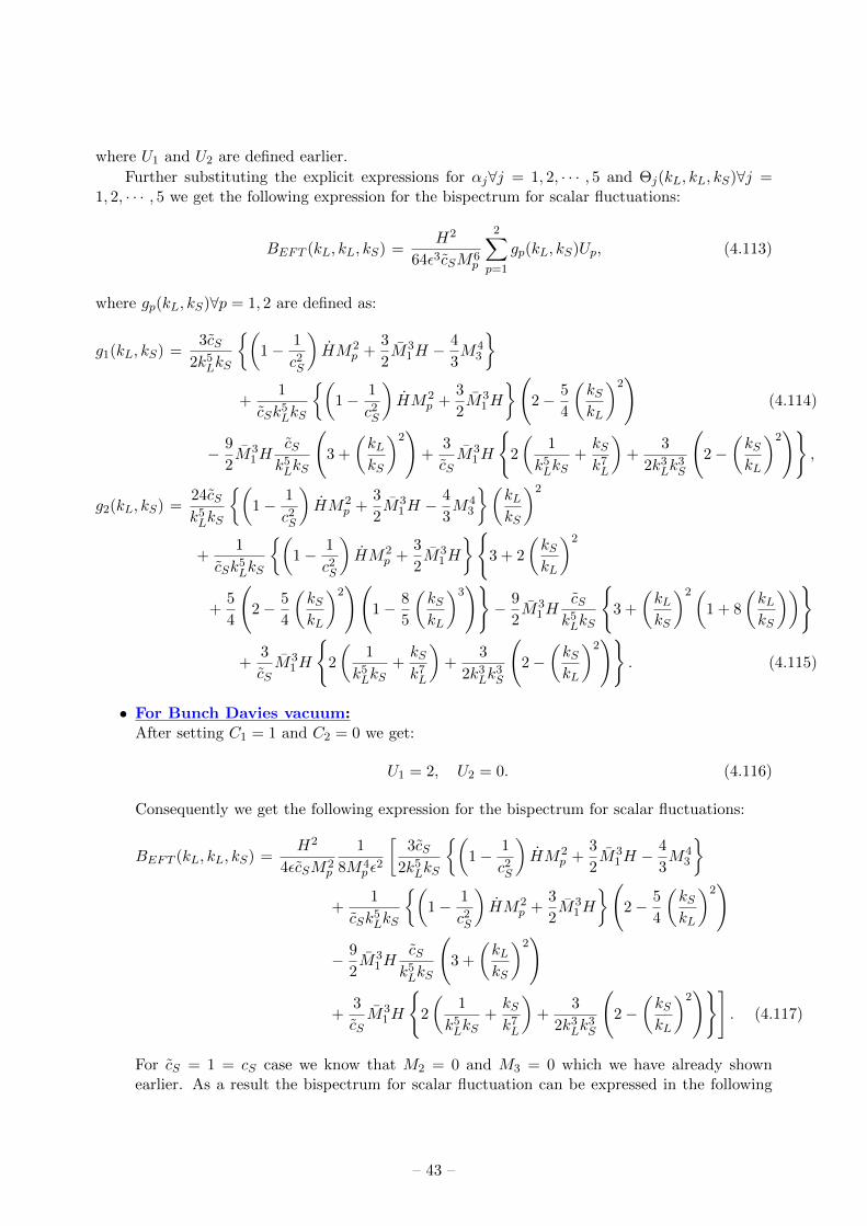
where U1 and U2 are defined earlier.

Further substituting the explicit expressions for αj∀j = 1, 2, · · · , 5 and Θj(kL, kL, kS)∀j =1, 2, · · · , 5 we get the following expression for the bispectrum for scalar fluctuations:

BEFT (kL, kL, kS) =H2

64ε3cSM6p

2∑p=1

gp(kL, kS)Up, (4.113)

where gp(kL, kS)∀p = 1, 2 are defined as:

g1(kL, kS) =3cS

2k5LkS

(1− 1

c2S

)HM2

p +3

2M3

1H −4

3M4

3

+

1

cSk5LkS

(1− 1

c2S

)HM2

p +3

2M3

1H

(2− 5

4

(kSkL

)2)

(4.114)

− 9

2M3

1HcSk5LkS

(3 +

(kLkS

)2)

+3

cSM3

1H

2

(1

k5LkS

+kSk7L

)+

3

2k3Lk

3S

(2−

(kSkL

)2)

,

g2(kL, kS) =24cSk5LkS

(1− 1

c2S

)HM2

p +3

2M3

1H −4

3M4

3

(kLkS

)2

+1

cSk5LkS

(1− 1

c2S

)HM2

p +3

2M3

1H

3 + 2

(kSkL

)2

+5

4

(2− 5

4

(kSkL

)2)(

1− 8

5

(kSkL

)3)− 9

2M3

1HcSk5LkS

3 +

(kLkS

)2(1 + 8

(kLkS

))

+3

cSM3

1H

2

(1

k5LkS

+kSk7L

)+

3

2k3Lk

3S

(2−

(kSkL

)2)

. (4.115)

• For Bunch Davies vacuum:After setting C1 = 1 and C2 = 0 we get:

U1 = 2, U2 = 0. (4.116)

Consequently we get the following expression for the bispectrum for scalar fluctuations:

BEFT (kL, kL, kS) =H2

4εcSM2p

1

8M4p ε

2

[3cS

2k5LkS

(1− 1

c2S

)HM2

p +3

2M3

1H −4

3M4

3

+

1

cSk5LkS

(1− 1

c2S

)HM2

p +3

2M3

1H

(2− 5

4

(kSkL

)2)

− 9

2M3

1HcSk5LkS

(3 +

(kLkS

)2)

+3

cSM3

1H

2

(1

k5LkS

+kSk7L

)+

3

2k3Lk

3S

(2−

(kSkL

)2)]

. (4.117)

For cS = 1 = cS case we know that M2 = 0 and M3 = 0 which we have already shownearlier. As a result the bispectrum for scalar fluctuation can be expressed in the following

– 43 –

simplified form:

BEFT (kL, kL, kS) =H2

4εM2p

1

8M4p ε

2M3

1H

[9

4k5LkS

+3

2k5LkS

(2− 5

4

(kSkL

)2)

(4.118)

− 9

2

1

k5LkS

(3 +

(kLkS

)2)

+ 3

2

(1

k5LkS

+kSk7L

)+

3

2k3Lk

3S

(2−

(kSkL

)2)]

.

For cS < 1 and cS < 1 case one can also recast the bispectrum for scalar fluctuations in thefollowing simplified form:

BEFT (kL, kL, kS) =H2

4εcSM2p

1

8M4p ε

2M3

1H

[3cS

2k5LkS

3

2+

4

3

c3

c4+

2c2S

c4

+

1

cSk5LkS

2c2S

c4+

3

2

(2− 5

4

(kSkL

)2)

− 9

2

cSk5LkS

(3 +

(kLkS

)2)

+3

cS

2

(1

k5LkS

+kSk7L

)+

3

2k3Lk

3S

(2−

(kSkL

)2)]

. (4.119)

• For α, β vacuum:

After setting C1 = coshα and C2 = eiβ sinhα we get:

U1 = J1(α, β), U2 = J2(α, β), (4.120)

where J1(α, β) and J2(α, β) are defined earlier.

Consequently we get the following expression for the bispectrum for scalar fluctuations:

BEFT (kL, kL, kS) =H2

4εcSM2p

1

16M4p ε

2[g1(kL, kS)J1(α, β) + g2(kL, kS)J2(α, β)] . (4.121)

For cS = 1 = cS case we know that M2 = 0 and M3 = 0 which we have already shown earlier.As a result the factors g1(kL, kS) and g2(kL, kS) appearing in the expression for bispectrumfor scalar fluctuation can be expressed in the following simplified form:

g1(kL, kS) =9

4k5LkS

M31H +

3

2k5LkS

M31H

(2− 5

4

(kSkL

)2)

− 9

2M3

1H1

k5LkS

(3 +

(kLkS

)2)

+ 3M31H

2

(1

k5LkS

+kSk7L

)+

3

2k3Lk

3S

(2−

(kSkL

)2)

, (4.122)

– 44 –

g2(kL, kS) =36

k5LkS

M31H

(kLkS

)2

+3

2k5LkS

M31H

3 + 2

(kSkL

)2

+5

4

(2− 5

4

(kSkL

)2)(

1− 8

5

(kSkL

)3)

− 9

2M3

1H1

k5LkS

3 +

(kLkS

)2(1 + 8

(kLkS

))

+ 3M31H

2

(1

k5LkS

+kSk7L

)+ +

3

2k3Lk

3S

(2−

(kSkL

)2)

. (4.123)

For cS < 1 and cS < 1 case one can also recast the factors g1(kL, kS) and g2(kL, kS) asappearing in the expression for bispectrum for scalar fluctuations in the following simplifiedform:

g1(kL, kS) =3cS

2k5LkS

3

2+

4

3

c3

c4+

2c2S

c4

+

1

cSk5LkS

2c2S

c4+

3

2

(2− 5

4

(kSkL

)2)

− 9

2M3

1HcSk5LkS

(3 +

(kLkS

)2)

+3

cSM3

1H

2

(1

k5LkS

+kSk7L

)+

3

2k3Lk

3S

(2−

(kSkL

)2)

, (4.124)

g2(kL, kS) =24cSk5LkS

3

2+

4

3

c3

c4+

2c2S

c4

(kLkS

)2

+1

cSk5LkS

2c2S

c4+

3

2

3 + 2

(kSkL

)2

+5

4

(2− 5

4

(kSkL

)2)(

1− 8

5

(kSkL

)3)

− 9

2M3

1HcSk5LkS

3 +

(kLkS

)2(1 + 8

(kLkS

))

+3

cSM3

1H

2

(1

k5LkS

+kSk7L

)+ +

3

2k3Lk

3S

(2−

(kSkL

)2)

. (4.125)

5 Determination of EFT coefficients and future predictions

In this section we compute the exact analytical expression for the EFT coefficients for two specificcases- 1. Canonical single field slow roll inflation and 2. General single field P (X,φ) models ofinflation, where X = −1

2gµν∂µφ∂νφ is the kinetic term. To determine the EFT coefficients for

canonical single field slow roll model or from general single field P (X,φ) model of inflation we willfollow the following strategy:

1. First of all, we will start with the general expression for the three point function and thebispectrum for scalar perturbations with arbitrary choice of quantum vacuum. Then we takethe Bunch-Davies and α, β vacuum to match with the standard results of scalar three pointfunction.

– 45 –

2. Next we take the equilateral limit and squeezed limit configuration of the bispectrum obtainedfrom single fleid slow roll model and general single field P (X,φ) model.

3. Further we equate the equilateral limit and squeezed limit configuration of the bispectrumcomputed from the EFT of inflation with the single field slow roll or from general single fieldP (X,φ) model.

4. Finally, for sound speed cS = 1 and cS < 1 we get the analytical expressions for all the EFTcoefficients for canonical single field slow roll models or from generalized single field P (X,φ)models of inflation.

5.1 For canonical Single Field Slow Roll inflation

Here our prime objective is to derive the EFT coefficients by computing the most general expressionfor the three point function for scalar fluctuations from the canonical single field slow roll model ofinflation for arbitrary vacuum. Then we give specific example for Bunch-Davies and α, β vacuumfor completeness.

5.1.1 Basic setup

Let us start with the action for single scalar field (inflaton) which has canonical kinetic term asgiven by:

Canonical model : S =

∫d4x√−g

[M2p

2R+X − V (φ)

], (5.1)

where V (φ) is the potential which satisfies slow-roll condition for inflation.

It is important to mention here that perturbations to the homogeneous situation discussedabove are introduced in the ADM formalism ehere the metric takes the form [30]:

ADM metric : ds2 = −N2dt2 + gij(dxi +N idt

) (dxj +N jdt

), (5.2)

where gij is the metric on the spatial three surface characterized by t, lapse N and shift Ni. Herewe choose synchronous gauge to maintain diffeomorphism invariance of the theory where the gaugefixing conditions are given by:

Synchronous gauge : N = 1, N i = 0 , (5.3)

and the perturbed metric is given by:

gij = a2(t) [(1 + 2ζ(t,x))δij + γij ] , γii = 0 , (5.4)

where ζ(t,x) and γij are defined earlier. Here it is important to note that, the structure of gijis exactly same that we have mentioned in case of EFT framework discussed in this paper. Notethat in the context of ADM formalism one can treat the scalar field φ, induced metric gij as thedynamical variables. On the other hand, N and N i mimics the role of Lagrange multipliers inADM formalism. Consequently, one needs to impose the equations of motion of N,N i as additionalconstraints in the synchronous gauge where the gauge condition as stated in Eq. (5.3) holds goodperfectly. More precisely, in this context the equations of motion of N and N i correspond to timeand spatial reparametrization invariance.

– 46 –

Further using the ADM metric as stated in Eq (5.2), the action for the single scalar fieldEq (5.1) can be recast as [30]:

S =

∫d4x√−g

[M2p

2N (3)R−NV +

1

2N

(EijE

ij − E2)

+1

2N

(φ−N i∂iφ

)2−Ngij∂iφ∂jφ

], (5.5)

where (3)R is the Ricci scalar curvature of the spatial slice. Also here Eij and E is defined as [30]:

Eij : =1

2(gij −∇iNj −∇jNi) = NKij , (5.6)

E : = Eii = gijEij = gijg

imgjnEmn = NgijgimgjnKmn. (5.7)

Here the covarinat derivative ∇i, is taken with respect to the 3-metric gij . Also in this contextthe extrinsic curvature Kij is defined as [30]:

Kij =1

NEij =

1

2N(gij −∇iNj −∇jNi) . (5.8)

Additionally we choose the following two gauges:

Gauge I : δφ(t,x) = 0, ζ(t,x) 6= 0, ∂iγij = 0, γii = 0 . (5.9)

Gauge II : δφ(t,x) 6= 0, ζ(t,x) = 0, ∂iγij = 0, γii = 0 . (5.10)

For our present computations, we will work in Gauge I as this is exactly same as the unitarygauge that we have used in the context of EFT framework. Also the tensor perturbation γij isexactly same for the unitary gauge that we have used for EFT setup.

5.1.2 Scalar three point function for Single Field Slow Roll inflation

Before computing the three point function for scalar mode fluctuation here it is important to notethat the two point function for Single Field Slow Roll inflation is exactly same with the resultsobtained for EFT of inflation with sound speed cS = 1 and cS = 1, which can be obtained bysetting the EFT coefficients, M2 = 0, M3 = 0, M1 6= 0, M4 6= 0, M2 6= 0, M3 6= 0, c5 = −1

2(1+ε) 20.Using three point function we can able to fix all of these coefficients.

20In case of Single Field Slow Roll inflation amplitude of power spectrum and spectral tilt for scalar fluctuationcan be written at the horizon crossing |kη| = 1 as:

For Bunch−Davies vacuum : ∆ζ(k∗) =

V (φ∗)

24π2 M4p εV

for dS

26εV −2ηV V (φ∗)

24π2 M4p εV (1 + εV )2

∣∣∣∣∣Γ( 32

+ 4εV − ηV )

Γ(32

) ∣∣∣∣∣2

for qdS.

For α, β vacuum : ∆ζ(k∗) =

V (φ∗)

24π2 M4p εV

[cosh 2α− sinh 2α cosβ] for dS

26εV −2ηV V (φ∗)

24π2 M4p εV (1 + εV )2

∣∣∣∣∣Γ( 32

+ 4εV − ηV )

Γ(32

) ∣∣∣∣∣2

[cosh 2α− sinh 2α cos (π (2 + 4εV − ηV ) + β)] for qdS.

andnζ(k∗)− 1 = 2ηV − 6εV . (5.11)

– 47 –

We here now proceed to calculate the three point function for the scalar fluctuation ζ(t,x)in the interacting picture with arbitrary vacuum. Then we cite results for Bunch-Davies and α, βvacuum. For Single Field Slow Roll inflation the third order term in the action Eq. (5.5) is givenby [30]:

S(3)ζ =

∫d4x

[a3ε2ζ

˙ζ2 + aε2ζ(∂ζ)2 − 2a3ε

˙ζ∂iζ∂i(ε∂

−2 ˙ζ)], (5.12)

which is derived from Eq (5.5) and here after neglecting all the contribution from the terms whichare subleading in the slow-roll parameters. Additionally here we use the following field redefinition:

ζ = ζ +ε− η

2

ζ2, (5.13)

where ε, η, δ and s are slow-roll parameters which are defined in the context of Single Field SlowRoll inflation as:

ε ∼ 1

2M2p

φ2

H2, η ∼ ε− δ, δ =

φ

Hφ, s = 0. (5.14)

Here one can also express the slow-roll parameters ε and η in terms of the slowly varying potentialV (φ) as, ε ∼ εV , η ∼ ηV − εV , δ ∼ 2εV − ηV . where the new slow-roll parameter εV and ηV are

defined as, εV =M2p

2

(V′(φ)

V (φ)

)2

, ηV = M2p

(V′′

(φ)V (φ)

). Here ′ represents d/dφ.

Now it is important to note that, in the present context of discussion we are interested in thethree point function for the scalar fluctuation field ζ, not for the redefined scalar field fluctuationζ and for this reason one can write down the exact connection between the three point fulction forthe scalar fluction field ζ and redefined scalar fluctuation field ζ in position space as:

〈ζ(x1)ζ(x2)ζ(x3)〉 = 〈ζ(x1)ζ(x2)ζ(x3)〉+ (2ε− η) [〈ζ(x1)ζ(x2)〉〈ζ(x1)ζ(x3)〉 (5.15)

+ 〈ζ(x2)ζ(x1)〉〈ζ(x2)ζ(x3)〉+ 〈ζ(x3)ζ(x1)〉〈ζ(x3)ζ(x2)〉] .

After taking the Fourier transform of the scalar fluction field ζ and redefined scalar fluctuationfield ζ one can express connection between three point function in momentum space and this isour main point of interest also.

The interaction Hamiltonian for the redefined scalar fluctuation ζ can be expressed as:

Hint =

∫d3x

[a ε2ζ ζ

′2 + a ε2ζ(∂ζ)2 − 2aεζ′∂iζ∂i(ε∂

−2ζ′)]. (5.16)

Further following the in-in formalism in interaction picture the expression for the three pointfunction for the redefined scalar fluctuation ζ and then transforming the final result in terms ofthe scalar fluctuation ζ in momentum one can write the following expression:

〈ζ(k1)ζ(k2)ζ(k3)〉 = −i∫ ηf=0

ηi=−∞dη a(η) 〈0| [ζ(ηf ,k1)ζ(ηf ,k2)ζ(ηf ,k3), Hint(η)] |0〉

= (2π)3δ(3)(k1 + k2 + k3)BSFSR(k1, k2, k3) ,

(5.17)

where BSFSR(k1, k2, k3) represents the bispectrum of scalar fluctuation ζ, which is computed fromSingle Field Slow Roll inflation. Here the final expression for the bispectrum of scalar fluctuation

– 48 –

for arbitray vacuum is given by:

BSFSR(k1, k2, k3) =H4

32ε2M4p

1

(k1k2k3)3

[2(2ε− η)

(|C1|2 + |C2|2

)2 3∑i=1

k3i

+ε(|C1|2 − |C2|2

)2− 3∑i=1

k3i +

3∑i,j=1,i 6=j

kik2j +

8

K

3∑i,j=1,i>j

k2i k

2j

+ε (C∗1C2 + C1C

∗2 )2

− 3∑i=1

k3i +

3∑i,j=1,i 6=j

kik2j

+ 83∑

i,j=1,i>j

k2i k

2j

3∑m=1

1

K − 2km

.

(5.18)

For Bunch Davies and α, β vacuum we get the following simplified expression for the bispec-trum for scalar fluctuation:

• For Bunch Davies vacuum:After setting C1 = 1 and C2 = 0 we get [30]:

BSFSR(k1, k2, k3) =H4

32ε2M4p

1

(k1k2k3)3

[2(2ε− η)

3∑i=1

k3i

+ε

− 3∑i=1

k3i +

3∑i,j=1,i 6=j

kik2j +

8

K

3∑i,j=1,i>j

k2i k

2j

. (5.19)

• For α, β vacuum:

After setting C1 = coshα and C2 = eiβ sinhα we get [32]:

BSFSR(k1, k2, k3) =H4

32ε2M4p

1

(k1k2k3)3

[2(2ε− η) cosh2 2α

3∑i=1

k3i

+ε

− 3∑i=1

k3i +

3∑i,j=1,i 6=j

kik2j +

8

K

3∑i,j=1,i>j

k2i k

2j

(5.20)

+ε sinh2 2α cos2 β

− 3∑i=1

k3i +

3∑i,j=1,i 6=j

kik2j + 8

3∑i,j=1,i>j

k2i k

2j

3∑m=1

1

K − 2km

.Further we consider equilateral limit and squeezed limit in which we finally get:

1. Equilateral limit configuration:Here the bispectrum for scalar perturbations in presence of arbitray quantum vacuum canbe expressed as:

BSFSR(k, k, k) =H4

32ε2M4p

1

k6

[6(2ε− η)

(|C1|2 + |C2|2

)2+ 11ε

(|C1|2 − |C2|2

)2+ 27ε (C∗1C2 + C1C

∗2 )2].

(5.21)

– 49 –

Now for Bunch Davies and α, β vacuum we get the following simplified expression for thebispectrum for scalar fluctuation:

• For Bunch Davies vacuum:After setting C1 = 1 and C2 = 0 we get:

BSFSR(k, k, k) =H4

32ε2M4p

1

k6[23ε− 6η] . (5.22)

• For α, β vacuum:

After setting C1 = coshα and C2 = eiβ sinhα we get:

BSFSR(k, k, k) =H4

32ε2M4p

1

k6

[6(2ε− η) cosh2 2α+ 11ε+ 27ε sinh2 2α cos2 β

]. (5.23)

2. Squeezed limit configuration:Here the bispectrum for scalar perturbations in presence of arbitray quantum vacuum canbe expressed as:

BSFSR(kL, kL, kS) =H4

32ε2M4p

1

k3Lk

3S

3∑j=−1

aj

(kSkL

)j, (5.24)

where the expansion coefficients aj∀j = −1, · · · , 3 for arbitrary vacuum are defined as:

a−1 = 16ε (C∗1C2 + C1C∗2 )2 ,

a0 = 4(2ε− η)(|C1|2 + |C2|2

)2+ 4ε

(|C1|2 − |C2|2

)2+ 4ε (C∗1C2 + C1C

∗2 )2 ,

a1 = 34ε (C∗1C2 + C1C∗2 )2 , a2 = 10ε

(|C1|2 − |C2|2

)2+ 10ε (C∗1C2 + C1C

∗2 )2 ,

a3 = 2(2ε− η)(|C1|2 + |C2|2

)2 − 5ε(|C1|2 − |C2|2

)2 − ε (C∗1C2 + C1C∗2 )2 .

Now for Bunch Davies and α, β vacuum we get the following simplified expression for thebispectrum for scalar fluctuation:

• For Bunch Davies vacuum:After setting C1 = 1 and C2 = 0, we get the following expression for the expansioncoefficients aj∀j = −1, · · · , 3:

a−1 = 0, a0 = 4(3ε− η), a1 = 0, a2 = 10ε, a3 = −(ε+ 2η). (5.25)

Consequently the bispectrum can be recast as:

BSFSR(kL, kL, kS) =H4

32ε2M4p

1

k3Lk

3S

[4(3ε− η) + 10ε

(kSkL

)2

− (ε+ 2η)

(kSkL

)3]. (5.26)

• For α, β vacuum:

After setting C1 = coshα and C2 = eiβ sinhα, we get the following expression for theexpansion coefficients aj∀j = −1, · · · , 3:

a−1 = 16ε sinh2 2α cos2 β, a0 = 4(2ε− η) cosh2 2α+ 4ε+ 4ε sinh2 2α cos2 β,

a1 = 34ε sinh2 2α cos2 β, a2 = 10ε+ 10ε sinh2 2α cos2 β,

a3 = 2(2ε− η) cosh2 2α− 5ε− ε sinh2 2α cos2 β.

– 50 –

Consequently the bispectrum can be recast as:

BSFSR(kL, kL, kS) =H4

32ε2M4p

1

k3Lk

3S

[16ε sinh2 2α cos2 β

(kSkL

)−1

+(4(2ε− η) cosh2 2α+ 4ε+ 4ε sinh2 2α cos2 β

)+ 34ε sinh2 2α cos2 β

(kSkL

)+(10ε+ 10ε sinh2 2α cos2 β

)(kSkL

)2

+(2(2ε− η) cosh2 2α− 5ε− ε sinh2 2α cos2 β

)(kSkL

)3].

(5.27)

5.1.3 Expression for EFT coefficients for Single Field Slow Roll inflation

Here our prime objective is to derive the analytical expressions for EFT coefficients for Single FieldSlow Roll inflation. To serve this purpose we start with a claim that the three point function andthe associated bispectrum for the scalar fluctuations computed from Single Field Slow Roll inflationis exactly same as that we have computed from EFT setup for consistent UV completion. Herewe use the equilateral limit and squeezed limit configurations to extract the analytical expressionfor the EFT coefficients. In the two limiting cases the results are following:

1. Equilateral limit configuration:For this case with arbitrary vacuum one can write:

BEFT (k, k, k) = BSFSR(k, k, k), (5.28)

which implies that:

M1 =

HM2

p ε[6(η−2ε)(|C1|2+|C2|2)

2−11ε(|C1|2−|C2|2)2−27ε(C∗1C2+C1C∗2)

2]

[ 12512U1+ 8073

196U2]

13

,

M2 ≈ M3 =

√M3

14Hc5

=

2M2

p ε[6(2ε−η)(|C1|2+|C2|2)

2+11ε(|C1|2−|C2|2)

2+27ε(C∗1C2+C1C∗2)

2]

(1+ε)[ 1253 U1+ 807349

U2]

12

,

c5 = −12 (1 + ε) , M2 = 0, M3 = 0,

M4 =(− c3c6HM3

1

) 14

=

c3H2M2

p ε[6(2ε−η)(|C1|2+|C2|2)

2+11ε(|C1|2−|C2|2)

2+27ε(C∗1C2+C1C∗2)

2]

c6[ 12512U1+ 8073

196U2]

14

.

(5.29)where for arbitrary vacuum U1 and U2 are defined as:

U1 =[(C1 − C2)3 (C∗31 + C∗32

)+ (C∗1 − C∗2 )3 (C3

1 + C32

)], (5.30)

U2 =[(C1 − C2)3C∗1C

∗2 (C∗1 − C∗2 ) + (C∗1 − C∗2 )3C1C2 (C1 − C2)

]. (5.31)

To constraint all these coefficients of EFT operators using CMB observation from PlanckTT+low P data we use [31]:

ε < 0.012 (95% CL), η = −0.0080+0.0088−0.0146 (68% CL), cS = 1 (95% CL),

H = Hinf ≤ 1.09× 10−4 Mp√ε cS , (5.32)

– 51 –

where Mp = 2.43 × 1018 GeV is the reduced Planck mass. Now for Bunch Davies and α, βvacuum we get the following simplified expression for the bispectrum for scalar fluctuation:

• For Bunch Davies vacuum:After setting C1 = 1 and C2 = 0 we get:

M1 =

6125HM

2p ε [6η − 23ε]

13 , M2 ≈ M3 =

√M3

14Hc5

=

3125(1+ε)M

2p ε [23ε− 6η]

12,

c5 = −12 (1 + ε) , M2 = 0, M3 = 0, M4 =

(− c3c6HM3

1

) 14

=

6c3125c6

H2M2p ε [23ε− 6η]

14.

(5.33)Further using the constraint stated in Eq (5.32) we finally get the following constraintson the coefficients of EFT operators:

1.23× 10−3 Mp < |M1| < 1.41× 10−3 Mp, 8.79× 10−3 Mp < |M2| ≈ |M3| < 1.08× 10−2 Mp,

M2 = 0, M3 = 0, 3.86× 10−4 Mp < M4 × (−c6/c3)1/4 < 4.29× 10−4 Mp. (5.34)

• For α, β vacuum:

After setting C1 = coshα and C2 = eiβ sinhα we get:

M1 =

HM2

p ε[6(η−2ε) cosh2 2α−11ε−27ε sinh2 2α cos2 β][ 12512

J1(α,β)+ 8073196

J2(α,β)]

13

,

M2 ≈ M3 =

√M3

14Hc5

=

2M2

p ε[6(2ε−η) cosh2 2α+11ε+27ε sinh2 2α cos2 β](1+ε)[ 1253 J1(α,β)+ 8073

49J2(α,β)]

12

,

c5 = −1

2(1 + ε) , M2 = 0, M3 = 0,

M4 =(− c3c6HM3

1

) 14

=

c3H2M2

p ε[6(2ε−η) cosh2 2α+11ε+27ε sinh2 2α cos2 β]c6[ 12512

J1(α,β)+ 8073196

J2(α,β)]

14

.

(5.35)

Further using the contraint stated in Eq (5.32) we finally get the following constraintson the coefficients of EFT operators for a given value of the parameters α and β (sayfor α = 0.1 and β = 0.1):

9.1× 10−4 Mp < |M1| < 1.1× 10−3 Mp, 1.11× 10−2 Mp < |M2| ≈ |M3| < 1.5× 10−2 Mp,

M2 = 0, M3 = 0, 3.06× 10−4 Mp < M4 × (−c6/c3)1/4 < 3.54× 10−4 Mp. (5.36)

2. Squeezed limit configuration:For this case with arbitrary vacuum one can write:

BEFT (kL, kL, kS) = BSFSR(kL, kL, kS), (5.37)

which implies that:

M1 =

2HM2

p ε

∑3j=−1 aj

(kSkL

)j∑3m=−1 bm

(kSkL

)m 1

3

, M2 ≈ M3 =

√M3

14Hc5

=

− M2

p ε

(1+ε)

∑3j=−1 aj

(kSkL

)j∑3m=−1 bm

(kSkL

)m 1

2

,

c5 = −12 (1 + ε) , M2 = 0, M3 = 0, M4 =

(− c3c6HM3

1

) 14

=

2H2M2

p ε c3c6

∑3j=−1 aj

(kSkL

)j∑3m=−1 bm

(kSkL

)m 1

4

.

(5.38)

– 52 –

where the expansion coefficients aj∀j = −1, · · · , 3 are defined earlier and here the coefficientsbm∀m = −1, · · · , 3 for arbitrary vacuum are defined as:

b−1 = −36U2, b0 =9

2(U1 + 9U2) , b1 = 0, b2 =

(27

4U1 +

17

2U2

), b3 = 0 , (5.39)

where U1 and U2 are already defined earlier.

Now for Bunch Davies and α, β vacuum we get the following simplified expression for thebispectrum for scalar fluctuation:

• For Bunch Davies vacuum:After setting C1 = 1 and C2 = 0, we get U1 = 2 and U2 = 0. Consequently theexpansion coefficients can be recast as:

a−1 = 0, a0 = 4(3ε− η), a1 = 0, a2 = 10ε, a3 = −(ε+ 2η) , (5.40)

and

b−1 = 0, b0 = 9, b1 = 0, b2 =27

2, b3 = 0 , (5.41)

Finally the EFT coefficients for scalar fluctuation can be written as:

M1 =

2HM2p ε

[4(3ε−η)+10ε

(kSkL

)2−(ε+2η)

(kSkL

)3][18− 27

2

(kSkL

)2]

13

,

M2 ≈ M3 =

√M3

14Hc5

=

M2p ε

[4(η−3ε)−10ε

(kSkL

)2+(ε+2η)

(kSkL

)3](1+ε)

[18− 27

2

(kSkL

)2]

12

,

c5 = −12 (1 + ε) , M2 = 0, M3 = 0,

M4 =(− c3c6HM3

1

) 14

=

2H2M2p ε c3

c6

[4(η−3ε)−10ε

(kSkL

)2+(ε+2η)

(kSkL

)3][18− 27

2

(kSkL

)2]

14

.

(5.42)

Further using the contraint stated in Eq (5.32) we finally get the following constraintson the coefficients of EFT operators for a given value of the parameter kS/kL (say forkS/kL = 0.1):

1.22× 10−3 Mp < |M1| < 1.56× 10−3 Mp, 8.67× 10−3 Mp < |M2| ≈ |M3| < 1.25× 10−2 Mp,

M2 = 0, M3 = 0, 3.75× 10−4 Mp < M4 × (−c6/c3)1/4 < 4.51× 10−4 Mp. (5.43)

• For α, β vacuum:

After setting C1 = coshα and C2 = eiβ sinhα, we get U1 = J1(α, β) and U2 = J2(α, β).Consequently the expansion coefficients can be recast as:

a−1 = 16ε sinh2 2α cos2 β, a0 = 4(2ε− η) cosh2 2α+ 4ε+ 4ε sinh2 2α cos2 β,

a1 = 34ε sinh2 2α cos2 β, a2 = 10ε+ 10ε sinh2 2α cos2 β,

a3 = 2(2ε− η) cosh2 2α− 5ε− ε sinh2 2α cos2 β. (5.44)

– 53 –

and

b−1 = −36J2(α, β), b0 =9

2(J1(α, β) + 9J2(α, β)) ,

b2 =

(27

4J1(α, β) +

17

2J2(α, β)

), b3 = 0 = b1. (5.45)

Finally the EFT coefficients for scalar fluctuation can be written as:

M1 =

2HM2

p ε

[−36J2(α, β)

(kSkL

)−1+ 9

(J1(α, β) + J2(α,β)

2

)−3

4 (9J1(α, β)− 7J2(α, β))(kSkL

)2]−1

[16ε sinh2 2α cos2 β

(kSkL

)−1+(4(2ε− η) cosh2 2α+ 4ε+ 4ε sinh2 2α cos2 β

)+34ε sinh2 2α cos2 β

(kSkL

)+(10ε+ 10ε sinh2 2α cos2 β

) (kSkL

)2

+(2(2ε− η) cosh2 2α− 5ε− ε sinh2 2α cos2 β

) (kSkL

)3] 1

3

,

M2 ≈ M3 =

√M3

14Hc5

=

M2p ε

(1+ε)

[36J2(α, β)

(kSkL

)−1− 9

(J1(α, β) + J2(α,β)

2

)+3

4 (9J1(α, β)− 7J2(α, β))(kSkL

)2]−1

[16ε sinh2 2α cos2 β

(kSkL

)−1+(4(2ε− η) cosh2 2α+ 4ε+ 4ε sinh2 2α cos2 β

)+34ε sinh2 2α cos2 β

(kSkL

)+(10ε+ 10ε sinh2 2α cos2 β

) (kSkL

)2

+(2(2ε− η) cosh2 2α− 5ε− ε sinh2 2α cos2 β

) (kSkL

)3] 1

2

,

c5 = −12 (1 + ε) , M2 = 0, M3 = 0,

M4 =(− c3c6HM3

1

) 14

=

2H2M2

p ε c3c6

[36J2(α, β)

(kSkL

)−1− 9

(J1(α, β) + J2(α,β)

2

)+3

4 (9J1(α, β)− 7J2(α, β))(kSkL

)2]−1

[16ε sinh2 2α cos2 β

(kSkL

)−1+(4(2ε− η) cosh2 2α+ 4ε+ 4ε sinh2 2α cos2 β

)+34ε sinh2 2α cos2 β

(kSkL

)+(10ε+ 10ε sinh2 2α cos2 β

) (kSkL

)2

+(2(2ε− η) cosh2 2α− 5ε− ε sinh2 2α cos2 β

) (kSkL

)3] 1

4

.

(5.46)

Further using the contraint stated in Eq (5.32) we finally get the following constraintson the coefficients of EFT operators for a given value of the parameters α, β and kS/kL(say for α = 0.1, β = 0.1 and kS/kL = 0.1):

6.05× 10−4 Mp < |M1| < 7.15× 10−4 Mp, 3.03× 10−3 Mp < |M2| ≈ |M3| < 3.89× 10−3 Mp,

M2 = 0, M3 = 0, 2.22× 10−3 Mp < M4 × (−c6/c3)1/4 < 2.51× 10−3 Mp. (5.47)

– 54 –

5.2 For General Single Field P (X,φ) inflation

Here our prime objective is to derive the EFT coefficients by computing the most general expressionfor the three point function for scalar fluctuations from the General Single Field P (X,φ) model ofinflation for arbitrary vacuum. Then we give specific example for Bunch-Davies and α, β vacuumfor completeness.

5.2.1 Basic setup

Let us start with the action for single scalar field (inflaton) which is described by the generalfunction P (X,φ), contains non canonical kinetic term in general and it is minimally coupled tothe gravity [32, 43]:

S =

∫d4x√−g

[M2p

2R+ P (X,φ)

]. (5.48)

In case of general structure of P (X,φ) the pressure p, the energy density ρ and effective speed ofsound parameter cS can be written as [43]:

p = P (X,φ), ρ = 2XP,X(X,φ)− P (X,φ), cS =

√P,X(X,φ)

P,X(X,φ) + 2XP,XX(X,φ). (5.49)

In case of general P (X,φ) theory the slow roll parameters can be expressed as [43]:

ε =XPX(X,φ)

H2M2p

, η = ε− δ

P,X(X,φ)[P,X(X,φ) +XP,XX(X,φ)] ,

s =2Xδ

P,X(X,φ)

[XP 2

,XX(X,φ)− P,X(X,φ)P,XX(X,φ)−XP,X(X,φ)P,XXX(X,φ)]

[P,X(X,φ) +XP,XX(X,φ)]. (5.50)

In case of Single Field Slow Roll inflation we have:

P (X,φ) = X − V (φ), (5.51)

where V (φ) is the single field slowly varying potential. For this case if we compute the effectivesound speed then it turns out to be cS = 1, which is consistent with our result obtained in theprevious section. Also if we compute the expressions for the slow roll parameters ε, η, δ and s theresults are also perfectly matches with the results obtained in Eq (5.14).

Similarly in case DBI inflationary model one can identify the function P (X,φ) as [44]:

P (X,φ) = − 1

f(φ)

√1− 2Xf(φ) +

1

f(φ)− V (φ), (5.52)

where the inflaton φ is identified to be the position of a D3 barne which is moving in warpedthroat geometry and f(φ) characterize the warp factor 21. For the effective potential V (φ) one canconsider following mathematical structures of the potentials in the UV and IR regime [44]:

• UV regime: In this case the inflaton moves from the UV regime of the warped geometric

space to the IR regime under the influence of the effective potential, V (φ) ' 12m

2φ2, where

the inflaton mass satisfy the constraint m >> Mp

√λ. In this specific situation the inflaton

starts rolling very far away from the origin of the effective potential and then rolls down ina relativistic fashion to the minimum of potential situated at the origin.

21For AdS like throat geometry, f(φ) ≈ λφ4 , where λ is the parameter in string theory which depends on the flux

number.

– 55 –

• IR regime: In this case the inflaton started moving from the IR regime of the warped space

geometry to the UV regime under the influence of the effective potential, V (φ) ' V0− 12m

2φ2,where the inflaton mass is comparable to the scale of inflation, as given by, m ≈ H. In thisspecific situation, the inflaton starts rolling down near the origin of the effective potentialand rolls down in a relativistic fashion away from it.

In case of DBI model the pressure p and the energy density ρ can be written as [44]:

p =1

f(φ)(1− cS)− V (φ), ρ =

1

f(φ)

(1

cS− 1

)+ V (φ), cS =

√1− 2Xf(φ) =

√1− φ2f(φ), (5.53)

where X = φ2/2. In this context the slow roll parameter [44]:

ε =3φ2

2[cSV (φ) + 1

f(φ)(1− cS)] ≈ 3

2 [1 + cSf(φ)V (φ)]. (5.54)

is not small and as a result the effective sound speed is very small, cS << 1. Consequently theinflaon speed during inflation is given by the expression, φ = ± 1√

f(φ). Additionally it is important

to note that in the context of DBI inflation the other slow roll parameters η and s can be computedas:

η ≈

[3√

1 + cSf(φ)V (φ) +

√3f(φ)cS

2 MpφcS

f(φ)V

′(φ) + V (φ)f

′(φ)− 1

2c2S

(2φf(φ) + φ2f

′(φ))]

[1 + cSf(φ)V (φ)]32

,

s = −√

3f(φ)cS2c2S

Mpφ[2φf(φ) + φ2f

′(φ)]. (5.55)

In the slow roll regime to validate slow-roll approximation along with cS << 1 we need to satisfythe constraint condition for DBI inflation, 2cSf(φ)V (φ) >> 1.

5.2.2 Scalar three point function for General Single Field P (X,φ) inflation

Before computing the three point function for scalar mode fluctuation here it is important to notethat the two point function for General Single Field P (X,φ) inflation is exactly same with theresults obtained for EFT of inflation with sound speed cS << 1 and cS << 1, which can beobtained by setting the EFT coefficients, M2 6= 0, M3 6= 0, M1 6= 0, M4 6= 0, M2 6= 0, M3 6= 0,c5 6= −1

2(1 + ε) 22. Using three point function we can able to fix all of these coefficients.

Now here before going to the details of the computation for three point function just using theknowledge of two two point function we can easily identify the exact analytical expression for theEFT coeficient M2. For this we need to identify the effective sound speed computed from GeneralSingle Field P (X,φ) inflation with the result obtained for the proposed EFT setup. Consequently

22In case of General Single Field P (X,φ) inflation amplitude of power spectrum and spectral tilt for scalarfluctuation can be written at the horizon crossing |kcSη| = 1 as:

For Bunch−Davies vacuum : ∆ζ(k∗) =

2X∗P,X(X∗, φ∗)− P (X∗, φ∗)

24π2 M4p cSε

for dS

23ε−η+ s2

2X∗P,X(X∗, φ∗)− P (X∗, φ∗)

24π2 M4p ε(1 + ε)2

∣∣∣∣∣Γ( 32

+ 3ε− η + s2)

Γ(32

) ∣∣∣∣∣2

for qdS.

– 56 –

we get:

M2 =

(−XP,XX(X,φ)

P,X(X,φ)HM2

p

) 14

=

0 for Single Field Slow Roll[(

φ2f(φ)

φ2f(φ)− 1

)HM2

p

2

] 14

for DBI.

(5.57)

We here now proceed to calculate the three point function for the scalar fluctuation ζ(t,x) in theinteracting picture with arbitrary vacuum in case of General Single Field P (X,φ) inflation. Thenwe cite results for Bunch-Davies and α, β vacuum and give a specific example for DBI model ofinflation.

Here we introduce two new parameters [43]:

Σ1(X,φ) = XP,X(X,φ) + 2X2P,XX(X,φ) =εH2M2

p

c2S

, (5.58)

Σ2(X,φ) = X2P,XX(X,φ) +2

3X3P,XXX(X,φ). (5.59)

which will appear in the expression for three point function for the scalar fluctuation. For Sin-gle Field Slow Roll inflation and DBI inflation we get the following expressions for theseparameters [43]:

Σ1(X,φ) =

X = εH2M2

p for Single Field Slow Roll

X

(1− 2Xf(φ))32

=εH2M2

p

c2S

for DBI.(5.60)

Σ2(X,φ) =

0 for Single Field Slow Roll

X2f(φ)

(1− 2Xf(φ))52

for DBI.(5.61)

For General Single Field P (X,φ) inflation the third order term in the action Eq. (5.48) is givenby [43]:

S(3)ζ =

∫d4x

[−a3

Σ1(X,φ)

(1− 1

c2S

)+ 2Σ2(X,φ)

˙ζ3

H3+a3ε(ε− 3 + 3c2

S

)c4S

ζ˙ζ2

+aε(ε− 2s+ 1− c2

S

)c2S

ζ(∂ζ)2 − 2a3ε˙ζ∂iζ∂i

(ε

c2S

∂−2 ˙ζ

)],

(5.62)

For α, β vacuum : ∆ζ(k∗) =

2X∗P,X(X∗, φ∗)− P (X∗, φ∗)

24π2 M4p cSε

[cosh 2α− sinh 2α cosβ] for dS

26ε−2η+s 2X∗P,X(X∗, φ∗)− P (X∗, φ∗)

24π2 M4p ε(1 + ε)2

∣∣∣∣∣Γ( 32

+ 3ε− η + s2)

Γ(32

) ∣∣∣∣∣2

[cosh 2α− sinh 2α cos

(π(

2 + 3ε− η +s

2

)+ β

)]for qdS.

andnζ(k∗)− 1 = 2η − 6ε− s. (5.56)

– 57 –

which is derived from Eq (5.5) and here after neglecting all the contribution from the terms whichare sub-leading in the slow-roll parameters. Additionally here we use the following field redefinition:

ζ = ζ +1

c2S

ε− η

2

ζ2, (5.63)

where ε, η, δ and s are already defined earlier for General Single Field P (X,φ) inflation.

Now it is important to note that, in the present context of discussion we are interested in thethree point function for the scalar fluctuation field ζ, not for the redefined scalar field fluctuationζ and for this reason one can write down the exact connection between the three point fulction forthe scalar fluction field ζ and redefined scalar fluctuation field ζ in position space as:

〈ζ(x1)ζ(x2)ζ(x3)〉 = 〈ζ(x1)ζ(x2)ζ(x3) +(2ε− η)

c2S

[〈ζ(x1)ζ(x2)〉〈ζ(x1)ζ(x3)〉

+ 〈ζ(x2)ζ(x1)〉〈ζ(x2)ζ(x3)〉+ 〈ζ(x3)ζ(x1)〉〈ζ(x3)ζ(x2)〉] . (5.64)

After taking the Fourier transform of the scalar fluctuation field ζ and redefined scalar fluctuationfield ζ one can express connection between three point function in momentum space and this isour main point of interest also.

The interaction Hamiltonian for the redefined scalar fluctuation ζ can be expressed as:

Hint =

∫d3x

[−

Σ1(X,φ)

(1− 1

c2S

)+ 2Σ2(X,φ)

ζ′3

H3+a ε(ε− 3 + 3c2

S

)c4S

ζ ζ′2

+a ε(ε− 2s+ 1− c2

S

)c2S

ζ(∂ζ)2 − 2aζ′∂iζ∂i

(ε

c2S

∂−2ζ′)]

. (5.65)

Further following the in-in formalism in interaction picture the expression for the three pointfunction for the redefined scalar fluctuation ζ and then transforming the final result in terms ofthe scalar fluctuation ζ in momentum one can write the following expression:

〈ζ(k1)ζ(k2)ζ(k3)〉 = −i∫ ηf=0

ηi=−∞dη a(η) 〈0| [ζ(ηf ,k1)ζ(ηf ,k2)ζ(ηf ,k3), Hint(η)] |0〉

= (2π)3δ(3)(k1 + k2 + k3)BGSF (k1, k2, k3),

(5.66)

where BGSF (k1, k2, k3) represents the bispectrum of scalar fluctuation ζ, which is computed fromGeneral Single Field P (X,φ) inflation. Here the final expression for the bispectrum of scalar

– 58 –

fluctuation for arbitray vacuum is given by:

BGSF (k1, k2, k3) =H4

32ε2M4p

1

(k1k2k3)3

[3

2

(1

c2S

− 1− 2Σ2(X,φ)

Σ1(X,φ)

)(|C1|2 + |C2|2

)2 (k1k2k3)2

K3

+

(1

c2S

− 1

)(|C1|2 + |C2|2

)2 3∑i=1

k3i +

4

K2

3∑i,j=1,i 6=j

k2i k

3j −

8

K

3∑i,j=1,i>j

k2i k

2j

+s

c2S

(|C1|2 + |C2|2

)2−2

3∑i=1

k3i +

4

K2

3∑i,j=1,i 6=j

k2i k

3j −

8

K

3∑i,j=1,i>j

k2i k

2j

+2(2ε− η)

(|C1|2 + |C2|2

)2 3∑i=1

k3i

+ε(|C1|2 − |C2|2

)2− 3∑i=1

k3i +

3∑i,j=1,i 6=j

kik2j +

8

K

3∑i,j=1,i>j

k2i k

2j

+ε (C∗1C2 + C1C

∗2 )2(−∑3

i=1 k3i +

∑3i,j=1,i 6=j kik

2j

+ 83∑

i,j=1,i>j

k2i k

2j

3∑m=1

1

K − 2km

+O(ε)

,

(5.67)

where O(ε) characterizes the sub-leading corrections in the three point function for the scalarfluctuation computed from General Single Field P (X,φ) inflation.

Now further we consider a very specific class of models, where the following constraint condi-tion 23P,Xφ(X,φ) = 0 perfectly holds good. In this case one can write down the following simplifiedexpression for the bispectrum of scalar fluctuation for arbitray vacuum as:

BGSF (k1, k2, k3) =H4

32ε2M4p

1

(k1k2k3)3

[(1

c2S

− 1− sε

3εX

)(|C1|2 + |C2|2

)2 (k1k2k3)2

K3

+

(1

c2S

− 1

)(|C1|2 + |C2|2

)2 3∑i=1

k3i +

4

K2

3∑i,j=1,i 6=j

k2i k

3j −

8

K

3∑i,j=1,i>j

k2i k

2j

+2(2ε− η)

(|C1|2 + |C2|2

)2 3∑i=1

k3i

+ε(|C1|2 − |C2|2

)2− 3∑i=1

k3i +

3∑i,j=1,i 6=j

kik2j +

8

K

3∑i,j=1,i>j

k2i k

2j

+ε (C∗1C2 + C1C

∗2 )2

− 3∑i=1

k3i +

3∑i,j=1,i 6=j

kik2j + 8

3∑i,j=1,i>j

k2i k

2j

3∑m=1

1

K − 2km

,

(5.68)

23Strictly speaking, DBI model is one of the exceptions where this condition is not applicable. On the other hand,in case of Single Field Slow Roll inflation this condition is applicable. But in that case one can set cS = 1 and getback all the results derived in the earlier section. Additionally it is important to mention that, here we considerthose models also where cS << 1 alongwith this given constraint.

– 59 –

where the new parameter εX is defined as 24:

εX = −XH,X

H2. (5.70)

For Bunch Davies and α, β vacuum we get the following simplified expression for the bispectrumfor scalar fluctuation:

• For Bunch Davies vacuum:After setting C1 = 1 and C2 = 0 we get [43]:

BGSF (k1, k2, k3) =H4

32ε2M4p

1

(1k2k3)3

[3

2

(1

c2S

− 1− 2Σ2(X,φ)

Σ1(X,φ)

)(k1k2k3)2

K3

+

(1

c2S

− 1

) 3∑i=1

k3i +

4

K2

3∑i,j=1,i 6=j

k2i k

3j −

8

K

3∑i,j=1,i>j

k2i k

2j

+s

c2S

−23∑i=1

k3i +

4

K2

3∑i,j=1,i 6=j

k2i k

3j −

8

K

3∑i,j=1,i>j

k2i k

2j

+2(2ε− η)

3∑i=1

k3i

+ε

− 3∑i=1

k3i +

3∑i,j=1,i 6=j

kik2j +

8

K

3∑i,j=1,i>j

k2i k

2j

.

(5.71)

Further for restricted class of General Single Field P (X,φ) model, which satisfies the con-straint P,Xφ(X,φ) = 0, one can further write down the following expression for the bispec-trum:

BGSF (k1, k2, k3) =H4

32ε2M4p

1

(k1k2k3)3

[(1

c2S

− 1− sε

3εX

)(k1k2k3)2

K3

+

(1

c2S

− 1

) 3∑i=1

k3i +

4

K2

3∑i,j=1,i 6=j

k2i k

3j −

8

K

3∑i,j=1,i>j

k2i k

2j

+2(2ε− η)

3∑i=1

k3i

+ε

− 3∑i=1

k3i +

3∑i,j=1,i 6=j

kik2j +

8

K

3∑i,j=1,i>j

k2i k

2j

,

(5.72)

• For α, β vacuum:

24For Single Field Slow Roll inflation the newly introduced parameter εX is computed as:

εX = ε(η − ε) ≈ εV (ηV − 2εV ) . (5.69)

– 60 –

After setting C1 = coshα and C2 = eiβ sinhα we get [32]:

BGSF (k1, k2, k3) =H4

32ε2M4p

1

(k1k2k3)3

[3

2

(1

c2S

− 1− 2Σ2(X,φ)

Σ1(X,φ)

)cosh2 2α

(k1k2k3)2

K3

+

(1

c2S

− 1

)cosh2 2α

3∑i=1

k3i +

4

K2

3∑i,j=1,i 6=j

k2i k

3j −

8

K

3∑i,j=1,i>j

k2i k

2j

+s

c2S

cosh2 2α

−23∑i=1

k3i +

4

K2

3∑i,j=1,i 6=j

k2i k

3j −

8

K

3∑i,j=1,i>j

k2i k

2j

+2(2ε− η) cosh2 2α

3∑i=1

k3i + ε

− 3∑i=1

k3i +

3∑i,j=1,i 6=j

kik2j +

8

K

3∑i,j=1,i>j

k2i k

2j

+ε sinh2 2α cos2 β

− 3∑i=1

k3i +

3∑i,j=1,i 6=j

kik2j + 8

3∑i,j=1,i>j

k2i k

2j

3∑m=1

1

K − 2km

.

(5.73)

Further for restricted class of General Single Field P (X,φ) model, which satisfies the con-straint P,Xφ(X,φ) = 0, one can further write down the following expression for the bispec-trum:

BGSF (k1, k2, k3) =H4

32ε2M4p

1

(k1k2k3)3

[(1

c2S

− 1− sε

3εX

)cosh2 2α

(k1k2k3)2

K3

+

(1

c2S

− 1

)cosh2 2α

3∑i=1

k3i +

4

K2

3∑i,j=1,i 6=j

k2i k

3j −

8

K

3∑i,j=1,i>j

k2i k

2j

+2(2ε− η) cosh2 2α

3∑i=1

k3i + ε

− 3∑i=1

k3i +

3∑i,j=1,i 6=j

kik2j +

8

K

3∑i,j=1,i>j

k2i k

2j

+ε sinh2 2α cos2 β

− 3∑i=1

k3i +

3∑i,j=1,i 6=j

kik2j + 8

3∑i,j=1,i>j

k2i k

2j

3∑m=1

1

K − 2km

,

(5.74)

Further we consider equilateral limit and squeezed limit in which we finally get:

1. Equilateral limit configuration:Here the bispectrum for scalar perturbations in presence of arbitray quantum vacuum canbe expressed as:

BGSF (k, k, k) =H4

32ε2M4p

1

k6

[1

18

(1

c2S

− 1− 2Σ2(X,φ)

Σ1(X,φ)

)(|C1|2 + |C2|2

)2−7

3

(1

c2S

− 1

)(|C1|2 + |C2|2

)2 − 34

3

s

c2S

(|C1|2 + |C2|2

)2+6(2ε− η)

(|C1|2 + |C2|2

)2+ 11ε

(|C1|2 − |C2|2

)2+ 27ε (C∗1C2 + C1C

∗2 )2].

(5.75)

Further for restricted class of General Single Field P (X,φ) model, which satisfies the con-straint P,Xφ(X,φ) = 0, one can further write down the following expression for the bispec-

– 61 –

trum:

BGSF (k1, k2, k3) =H4

32ε2M4p

1

k6

[1

27

(1

c2S

− 1− sε

3εX

)(|C1|2 + |C2|2

)2 − 7

3

(1

c2S

− 1

)(|C1|2 + |C2|2

)2+6(2ε− η)

(|C1|2 + |C2|2

)2+ 11ε

(|C1|2 − |C2|2

)2+ 27ε (C∗1C2 + C1C

∗2 )2],

(5.76)

Now for Bunch Davies and α, β vacuum we get the following simplified expression for thebispectrum for scalar fluctuation:

• For Bunch Davies vacuum:After setting C1 = 1 and C2 = 0 we get:

BGSF (k, k, k) =H4

32ε2M4p

1

k6

[1

18

(1

c2S

− 1− 2Σ2(X,φ)

Σ1(X,φ)

)− 7

3

(1

c2S

− 1

)− 34

3

s

c2S

+ 23ε− 6η

].

(5.77)Further for restricted class of General Single Field P (X,φ) model, which satisfies theconstraint P,Xφ(X,φ) = 0, we get:

BGSF (k1, k2, k3) =H4

32ε2M4p

1

k6

[1

27

(1

c2S

− 1− sε

3εX

)− 7

3

(1

c2S

− 1

)+ 23ε− 6η

], (5.78)

• For α, β vacuum:

After setting C1 = coshα and C2 = eiβ sinhα we get:

BGSF (k, k, k) =H4

32ε2M4p

1

k6

[1

18

(1

c2S

− 1− 2Σ2(X,φ)

Σ1(X,φ)

)cosh2 2α

−7

3

(1

c2S

− 1

)cosh2 2α− 34

3

s

c2S

cosh2 2α

+6(2ε− η) cosh2 2α+ 11ε+ 27ε sinh2 2α cos2 β].

(5.79)

Further for restricted class of General Single Field P (X,φ) model, which satisfies theconstraint P,Xφ(X,φ) = 0, we get:

BGSF (k, k, k) =H4

32ε2M4p

1

k6

[1

27

(1

c2S

− 1− sε

3εX

)cosh2 2α− 7

3

(1

c2S

− 1

)cosh2 2α

+ 6(2ε− η) cosh2 2α+ 11ε+ 27ε sinh2 2α cos2 β].

(5.80)

2. Squeezed limit configuration:Here the bispectrum for scalar perturbations in presence of arbitray quantum vacuum canbe expressed as:

BGSF (kL, kL, kS) =H4

32ε2M4p

1

k3Lk

3S

3∑j=−1

tj

(kSkL

)j, (5.81)

– 62 –

where the expansion coefficients tj∀j = −1, · · · , 3 for arbitrary vacuum are defined as:

t−1 = 16ε (C∗1C2 + C1C∗2 )2 ,

t0 =

(4(2ε− η)− 6s

c2S

)(|C1|2 + |C2|2

)2+ 4ε

(|C1|2 − |C2|2

)2+ 4ε (C∗1C2 + C1C

∗2 )2 ,

t1 = 34ε (C∗1C2 + C1C∗2 )2 , (5.82)

t2 =

3

16

(1

c2S

− 1− 2Σ2(X,φ)

Σ1(X,φ)

)− 6

(1

c2S

− 1

)− 6s

c2S

(|C1|2 + |C2|2

)2+ 10ε

(|C1|2 − |C2|2

)2+ 10ε (C∗1C2 + C1C

∗2 )2 ,

t3 =

2(2ε− η)− 9

32

(1

c2S

− 1− 2Σ2(X,φ)

Σ1(X,φ)

)+ 5

(1

c2S

− 1

)+

2s

c2S

(|C1|2 + |C2|2

)2− 5ε

(|C1|2 − |C2|2

)2 − ε (C∗1C2 + C1C∗2 )2 .

Further for restricted class of General Single Field P (X,φ) model, which satisfies the con-straint P,Xφ(X,φ) = 0, we get:

t−1 = 16ε (C∗1C2 + C1C∗2 )2 ,

t0 = 4(2ε− η)(|C1|2 + |C2|2

)2+ 4ε

(|C1|2 − |C2|2

)2+ 4ε (C∗1C2 + C1C

∗2 )2 ,

t1 = 34ε (C∗1C2 + C1C∗2 )2 , (5.83)

t2 =

1

8

(1

c2S

− 1− sε

3εX

)− 6

(1

c2S

− 1

)(|C1|2 + |C2|2

)2+ 10ε

(|C1|2 − |C2|2

)2+ 10ε (C∗1C2 + C1C

∗2 )2 ,

t3 =

2(2ε− η)− 3

16

(1

c2S

− 1− sε

3εX

)+ 5

(1

c2S

− 1

)(|C1|2 + |C2|2

)2− 5ε

(|C1|2 − |C2|2

)2 − ε (C∗1C2 + C1C∗2 )2 .

Now for Bunch Davies and α, β vacuum we get the following simplified expression for thebispectrum for scalar fluctuation:

• For Bunch Davies vacuum:After setting C1 = 1 and C2 = 0, we get the following expression for the expansioncoefficients tj∀j = −1, · · · , 3:

t−1 = 0,

t0 = 4(3ε− η)− 6s

c2S

,

t1 = 0, (5.84)

t2 = 10ε+

3

16

(1

c2S

− 1− 2Σ2(X,φ)

Σ1(X,φ)

)− 6

(1

c2S

− 1

)− 6s

c2S

,

t3 = −(ε+ 2η) +

5

(1

c2S

− 1

)+

2s

c2S

− 9

32

(1

c2S

− 1− 2Σ2(X,φ)

Σ1(X,φ)

).

– 63 –

Consequently the bispectrum can be recast as:

BGSF (kL, kL, kS) =H4

32ε2M4p

1

k3Lk

3S

[4(3ε− η)− 6s

c2S

+

(10ε+

3

16

(1

c2S

− 1− 2Σ2(X,φ)

Σ1(X,φ)

)− 6

(1

c2S

− 1

)− 6s

c2S

)(kSkL

)2

+

(−(ε+ 2η) +

5

(1

c2S

− 1

)+

2s

c2S

− 9

32

(1

c2S

− 1− 2Σ2(X,φ)

Σ1(X,φ)

))(kSkL

)3].

(5.85)

Further for restricted class of General Single Field P (X,φ) model, which satisfies theconstraint P,Xφ(X,φ) = 0, we get:

t−1 = 0,

t0 = 4(3ε− η),

t1 = 0, (5.86)

t2 =

1

8

(1

c2S

− 1− sε

3εX

)− 6

(1

c2S

− 1

)+ 10ε,

t3 =

5

(1

c2S

− 1

)− 3

16

(1

c2S

− 1− sε

3εX

)− (ε+ 2η)

for such case bispectrum is given by:

BGSF (kL, kL, kS) =H4

32ε2M4p

1

k3Lk

3S

[4(3ε− η)

+

(1

8

(1

c2S

− 1− sε

3εX

)− 6

(1

c2S

− 1

)+ 10ε

)(kSkL

)2

+

(−(ε+ 2η) +

5

(1

c2S

− 1

)− 3

16

(1

c2S

− 1− sε

3εX

))(kSkL

)3].

(5.87)

• For α, β vacuum:

After setting C1 = coshα and C2 = eiβ sinhα, we get the following expression for theexpansion coefficients aj∀j = −1, · · · , 3:

t−1 = 16ε sinh2 2α cos2 β,

t0 =

(4(2ε− η)− 6s

c2S

)cosh2 2α+ 4ε+ 4ε sinh2 2α cos2 β,

t1 = 34ε sinh2 2α cos2 β, (5.88)

t2 =

3

16

(1

c2S

− 1− 2Σ2(X,φ)

Σ1(X,φ)

)− 6

(1

c2S

− 1

)− 6s

c2S

cosh2 2α

+ 10ε+ 10ε sinh2 2α cos2 β,

t3 =

2(2ε− η)− 9

32

(1

c2S

− 1− 2Σ2(X,φ)

Σ1(X,φ)

)+ 5

(1

c2S

− 1

)+

2s

c2S

cosh2 2α

− 5ε− ε sinh2 2α cos2 β.

– 64 –

Consequently the bispectrum can be recast as:

BGSF (kL, kL, kS) =H4

32ε2M4p

1

k3Lk

3S

[16ε sinh2 2α cos2 β

(kSkL

)−1

+((

4(2ε− η)− 6sc2S

)cosh2 2α+ 4ε+ 4ε sinh2 2α cos2 β

)+ 34ε sinh2 2α cos2 β

(kSkL

)+(

316

(1c2S− 1− 2Σ2(X,φ)

Σ1(X,φ)

)− 6

(1c2S− 1)− 6s

c2S

cosh2 2α

+ 10ε+ 10ε sinh2 2α cos2 β) (

kSkL

)2

+(

2(2ε− η)− 932

(1c2S− 1− 2Σ2(X,φ)

Σ1(X,φ)

)+ 5

(1c2S− 1)

+ 2sc2S

cosh2 2α

− 5ε− ε sinh2 2α cos2 β) (

kSkL

)3].

(5.89)

Further for restricted class of General Single Field P (X,φ) model, which satisfies theconstraint P,Xφ(X,φ) = 0, we get:

t−1 = 16ε sinh2 2α cos2 β,

t0 = 4(2ε− η) cosh2 2α+ 4ε+ 4ε sinh2 2α cos2 β,

t1 = 34ε sinh2 2α cos2 β, (5.90)

t2 =

1

8

(1

c2S

− 1− sε

3εX

)− 6

(1

c2S

− 1

)cosh2 2α

+ 10ε+ 10ε sinh2 2α cos2 β,

t3 =

2(2ε− η)− 3

16

(1

c2S

− 1− sε

3εX

)+ 5

(1

c2S

− 1

)cosh2 2α

− 5ε− ε sinh2 2α cos2 β.

Consequently the bispectrum can be recast as:

BGSF (kL, kL, kS) =H4

32ε2M4p

1

k3Lk

3S

[16ε sinh2 2α cos2 β

(kSkL

)−1

+(4(2ε− η) cosh2 2α+ 4ε+ 4ε sinh2 2α cos2 β

)+ 34ε sinh2 2α cos2 β

(kSkL

)+(

18

(1c2S− 1− sε

3εX

)− 6

(1c2S− 1)

cosh2 2α

+ 10ε+ 10ε sinh2 2α cos2 β) (

kSkL

)2

+(

2(2ε− η)− 316

(1c2S− 1− sε

3εX

)+ 5

(1c2S− 1)

cosh2 2α

− 5ε− ε sinh2 2α cos2 β) (

kSkL

)3].

(5.91)

– 65 –

5.2.3 Expression for EFT coefficients for General Single Field P (X,φ) inflation

Here our prime objective is to derive the analytical expressions for EFT coefficients for GeneralSingle Field P (X,φ) inflation. To serve this purpose here we start with a claim that the threepoint function and the associated bispectrum for the scalar fluctuations computed from GeneralSingle Field P (X,φ) inflation is exactly same as that we have computed from EFT setup. Herewe use the equilateral limit and squeezed limit configurations to extract the analytical expressionfor the EFT coefficients. In the two limiting cases the results are following:

1. Equilateral limit configuration:For this case with arbitrary vacuum one can write:

BEFT (k, k, k) = BGSF (k, k, k), (5.92)

which implies that 25:

M1 =

A

2BH

[−1 +

√1 + 4BC

A2

] 13

, M2 ≈ M3 =

√M3

14Hc5

=

√A

8BH2c5

[−1 +

√1 + 4BC

A2

],

M2 =(−XP,XX(X,φ)

P,X(X,φ) HM2p

) 14,

M3 =

− A

2B

c3c4

[−1 +

√1 + 4BC

A2

] 14

,

M4 =(− c3c6HM3

1

) 14

=

(− A

2B

c3c6

[−1 +

√1 + 4BC

A2

]) 14

.

(5.94)

where the factors A, B and C are defined as:

A =

(3

2+

4

3

c3

c4+

2c2S

c4

)[U1

27− 3U2

]− 5

2U1 +

99

98U2

−∆

4

[1

18

(1

c2S

− 1− 2Σ2(X,φ)

Σ1(X,φ)

)(|C1|2 + |C2|2

)2−7

3

(1

c2S

− 1

)(|C1|2 + |C2|2

)2 − 34

3

s

c2S

(|C1|2 + |C2|2

)2+6(2ε− η)

(|C1|2 + |C2|2

)2+ 11ε

(|C1|2 − |C2|2

)2+ 27ε (C∗1C2 + C1C

∗2 )2],

B =

(3

2+

4

3

c3

c4+

2c2S

c4

)[U1

27− 3U2

]− 5

2U1 +

99

98U2

∆c2

S

2εH2M2p

, (5.95)

C =H2M2

p εc2S

2

[1

18

(1

c2S

− 1− 2Σ2(X,φ)

Σ1(X,φ)

)(|C1|2 + |C2|2

)2−7

3

(1

c2S

− 1

)(|C1|2 + |C2|2

)2 − 34

3

s

c2S

(|C1|2 + |C2|2

)2+6(2ε− η)

(|C1|2 + |C2|2

)2+ 11ε

(|C1|2 − |C2|2

)2+ 27ε (C∗1C2 + C1C

∗2 )2].

25Here we also get another solution:

M1 =

A

2BH

[−1−

√1 +

4BC

A2

] 13

, (5.93)

which is redundant in the present context as this solution is not consistent with the cS = 1 and cS = 1 limit resultas computed in the earlier section for Single Field Slow Roll inflation.

– 66 –

Further for restricted class of General Single Field P (X,φ) model, which satisfies the con-straint P,Xφ(X,φ) = 0, we get the following expression for the factors A, B and C as:

A =

(3

2+

4

3

c3

c4+

2c2S

c4

)[U1

27− 3U2

]− 5

2U1 +

99

98U2

−∆

4

[1

27

(1

c2S

− 1− sε

3εX

)(|C1|2 + |C2|2

)2 − 7

3

(1

c2S

− 1

)(|C1|2 + |C2|2

)2+6(2ε− η)

(|C1|2 + |C2|2

)2+ 11ε

(|C1|2 − |C2|2

)2+ 27ε (C∗1C2 + C1C

∗2 )2],

B =

(3

2+

4

3

c3

c4+

2c2S

c4

)[U1

27− 3U2

]− 5

2U1 +

99

98U2

∆c2

S

2εH2M2p

, (5.96)

C =H2M2

p εc2S

2

[1

27

(1

c2S

− 1− sε

3εX

)(|C1|2 + |C2|2

)2 − 7

3

(1

c2S

− 1

)(|C1|2 + |C2|2

)2+6(2ε− η)

(|C1|2 + |C2|2

)2+ 11ε

(|C1|2 − |C2|2

)2+ 27ε (C∗1C2 + C1C

∗2 )2].

where for arbitrary vacucum U1 and U2 are defined as:

U1 =[(C1 − C2)3 (C∗31 + C∗32

)+ (C∗1 − C∗2 )3 (C3

1 + C32

)], (5.97)

U2 =[(C1 − C2)3C∗1C

∗2 (C∗1 − C∗2 ) + (C∗1 − C∗2 )3C1C2 (C1 − C2)

]. (5.98)

If we take cS = 1 and cS = 1 then we get then we get back all the results obtained for SingleField Slow Roll inflation in the previous section.

Now for Bunch Davies and α, β vacuum we get the following simplified expression for thebispectrum for scalar fluctuation:

• For Bunch Davies vacuum:After setting C1 = 1 and C2 = 0 we get the following expression for the factors A, Band C as:

A =2

27

(3

2+

4

3

c3

c4+

2c2S

c4

)− 5− ∆

4

[1

18

(1

c2S

− 1− 2Σ2(X,φ)

Σ1(X,φ)

)−7

3

(1

c2S

− 1

)− 34

3

s

c2S

+ (23ε− 6η)

],

B =

2

27

(3

2+

4

3

c3

c4+

2c2S

c4

)− 5

∆c2

S

2εH2M2p

, (5.99)

C =H2M2

p εc2S

2

[1

18

(1

c2S

− 1− 2Σ2(X,φ)

Σ1(X,φ)

)− 7

3

(1

c2S

− 1

)− 34

3

s

c2S

+ (23ε− 6η)

].

Further for restricted class of General Single Field P (X,φ) model, which satisfies theconstraint P,Xφ(X,φ) = 0, we get the following expression for the factors A, B and Cas:

A =2

27

(3

2+

4

3

c3

c4+

2c2S

c4

)− 5− ∆

4

[1

27

(1

c2S

− 1− sε

3εX

)− 7

3

(1

c2S

− 1

)+ (23ε− 6η)

],

B =

2

27

(3

2+

4

3

c3

c4+

2c2S

c4

)− 5

∆c2

S

2εH2M2p

, (5.100)

C =H2M2

p εc2S

2

[1

27

(1

c2S

− 1− sε

3εX

)− 7

3

(1

c2S

− 1

)+ (23ε− 6η)

].

– 67 –

• For α, β vacuum:

After setting C1 = coshα and C2 = eiβ sinhα we get the following expression for thefactors A, B and C as:

A =

(3

2+

4

3

c3

c4+

2c2S

c4

)[J1(α, β)

27− 3J2(α, β)

]− 5

2J1(α, β) +

99

98J2(α, β)

−∆

4

[1

18

(1

c2S

− 1− 2Σ2(X,φ)

Σ1(X,φ)

)− 7

3

(1

c2S

− 1

)− 34

3

s

c2S

cosh2 2α

+6(2ε− η) cosh2 2α+ 11ε+ 27ε sinh2 α cos2 β],

B =

(3

2+

4

3

c3

c4+

2c2S

c4

)[J1(α, β)

27− 3J2(α, β)

]− 5

2J1(α, β) +

99

98J2(α, β)

∆c2

S

2εH2M2p

, (5.101)

C =H2M2

p εc2S

2

[1

18

(1

c2S

− 1− 2Σ2(X,φ)

Σ1(X,φ)

)− 7

3

(1

c2S

− 1

)− 34

3

s

c2S

cosh2 2α

+6(2ε− η) cosh2 2α+ 11ε+ 27ε sinh2 α cos2 β].

Further for restricted class of General Single Field P (X,φ) model, which satisfies theconstraint P,Xφ(X,φ) = 0, we get the following expression for the factors A, B and Cas:

A =

(3

2+

4

3

c3

c4+

2c2S

c4

)[J1(α, β)

27− 3J2(α, β)

]− 5

2J1(α, β) +

99

98J2(α, β)

−∆

4

[1

27

(1

c2S

− 1− sε

3εX

)− 7

3

(1

c2S

− 1

)+ 6(2ε− η)

cosh2 2α

+ 11ε+ 27ε sinh2 α cos2 β],

B =

(3

2+

4

3

c3

c4+

2c2S

c4

)[J1(α, β)

27− 3J2(α, β)

]− 5

2J1(α, β) +

99

98J2(α, β)

∆c2

S

2εH2M2p

, (5.102)

C =H2M2

p εc2S

2

[1

27

(1

c2S

− 1− sε

3εX

)− 7

3

(1

c2S

− 1

)+ 6(2ε− η)

cosh2 2α

+ 11ε+ 27ε sinh2 α cos2 β].

2. Squeezed limit configuration:For this case with arbitray vacuum one can write:

BEFT (kL, kL, kS) = BGSF (kL, kL, kS), (5.103)

which implies that:

M1 =

A

2BH

[−1 +

√1 + 4BC

A2

] 13

, M2 ≈ M3 =

√M3

14Hc5

=

√A

8BH2c5

[−1 +

√1 + 4BC

A2

],

M2 =(−XP,XX(X,φ)

P,X(X,φ) HM2p

) 14, M3 =

− A

2B

c3c4

[−1 +

√1 + 4BC

A2

] 14

,

M4 =(− c3c6HM3

1

) 14

=

(− A

2B

c3c6

[−1 +

√1 + 4BC

A2

]) 14

.

(5.104)

– 68 –

where the factors A, B and C are defined as 26:

A = P1 + P2 −3∑

j=−1

tj

(kSkL

)j, B =

P1∆

2εH2M2p

, C = 2εH2M2p

3∑j=−1

tj

(kSkL

)j, (5.106)

where the expansion coefficients tj∀j = −1, · · · , 3 are defined earlier for general P (X,φ)model and also for restricted class of model where P,Xφ(X,φ) = 0 constarint satisfies.

Here the factors P1 and P2 are defined as:

P1 =3∑

m=−1

em

(kSkL

)m, P2 =

3∑m=−1

hm

(kSkL

)m, (5.107)

where the expansion coefficients em∀m = −1, · · · , 3 and hm∀m = −1, · · · , 3 for arbitraryvacuum are defined as:

e−1 = −36U2, e0 =

[−9

2U1 +

(24

3

2+

4

3

c3

c4+

2c2S

c4

− 9

2

)U2

],

e1 = 0, e2 =

[−27

2U2 +

(3

2

3

2+

4

3

c3

c4+

2c2S

c4

− 27

2

)U1

], e3 = 0, (5.108)

and

h−1 = 0, h0 =9

c2S

(U1 + U2) , h1 = 0,

h2 =

[(15 + 2

3

2+

2c2S

c4

)U1 +

(45

2+ 3

3

2+

2c2S

c4

)U2

], h3 = 0, (5.109)

where U1 and U2 are already defined earlier.

Now for Bunch Davies and α, β vacuum we get the following simplified expression for thebispectrum for scalar fluctuation:

• For Bunch Davies vacuum:After setting C1 = 1 and C2 = 0, we get U1 = 2 and U2 = 0. Consequently theexpansion coefficients can be recast as:

e−1 = 0, e0 = −9, e1 = 0, e2 = −27, e3 = 0, (5.110)

and

h−1 = 0, h0 =18

c2S

, h1 = 0, h2 =

(30 + 4

3

2+

2c2S

c4

), h3 = 0, (5.111)

26Here we also get another solution:

M1 =

A

2BH

−1−

√1 +

4BC

A2

13

, (5.105)

which is redundant in the present context as this solution is not consistent with the cS = 1 and cS = 1 limit resultas computed in the earlier section for General Single Field P (X,φ) inflation.

– 69 –

• For α, β vacuum:

After setting C1 = coshα and C2 = eiβ sinhα, we get U1 = J1(α, β) and U2 = J2(α, β).Consequently the expansion coefficients can be recast as:

e−1 = −36J2(α, β), e0 =

[−9

2J1(α, β) +

(24

3

2+

4

3

c3

c4+

2c2S

c4

− 9

2

)J2(α, β)

],

e1 = 0, e2 =

[−27

2J2(α, β) +

(3

2

3

2+

4

3

c3

c4+

2c2S

c4

− 27

2

)J1(α, β)

], e3 = 0, (5.112)

and

h−1 = 0, h0 =9

c2S

(U1 + J2(α, β)U2) , h1 = 0,

h2 =

[(15 + 2

3

2+

2c2S

c4

)J1(α, β) +

(45

2+ 3

3

2+

2c2S

c4

)J2(α, β)

], h3 = 0. (5.113)

6 Conclusion

To summarize, in this paper, we have addressed the following issues:

• We have derived the analytical expressions for the two point correlation function for scalarand tensor fluctuations and three point correlation function for scalar fluctuations from EFTframework in quasi de Sitter background in a model independent way. For this computationwe use an arbitrary quantum state as initial choice of vacuum. Such a choice finally give riseto the most general expressions for the two point and three point correlation functions forprimordial fluctuation in EFT. Further we have simplified our results by considering BunchDavies vacuum and α, β vacuum state.

• During our computation we have truncated the EFT action by considering the all possibletwo derivative terms in the metric. This allows us to derive correct expressions for the twopoint and three point correlation functions for EFT which are consistent with both singlefield slow roll model and generalized non-canonical P (X,φ) single field models minimallycoupled with gravity 27.

• Further we have derived the analytical expressions for the coefficients of all relevant EFToperators for single field slow roll model and generalized non-canonical P (X,φ) single fieldmodels. We have derived the results in terms of slow roll parameters, effective sound speedparameter and the constants which are fixed by the choice of arbitrary initial vacuum state.Next, we have simplified our results also presented the results by considering Bunch Daviesvacuum and α, β vacuum state.

• Finally using the CMB observation from Planck we constrain all of these EFT coefficientsfor various single field slow roll models and generalized non-canonical P (X,φ) models ofinflation.

The future directions of this paper are appended below point-wise:

27This is really an important outcome as the earlier derived results for the three point function for EFT in quaside Sitter background was not consistent with the known result for single field slow roll model, where effective soundspeed is fixed at cS = 1.

– 70 –

• One can further carry forward this work to compute four point scalar correlation functionfrom EFT framework using arbitrary initial choice of the quantum vacuum state. The presentwork can also be extended for the computation of the three point correlation from tensorfluctuation, other three point cross correlations between scalar and tensor mode fluctuationin the context of EFT with arbitrary initial vacuum.

• In the present EFT framework we have not considered the effects of any additional heavyfields (m >> H) in the effective action. One can redo the analysis with such additionaleffects in the EFT framework to study the quantum entanglement, cosmological decoherenceand Bell’s inequality violation in the context of primordial cosmology. Once acan also futhergeneralize this compuatation for any arbitrary spin fields which are consistent with theunitarity bound.

• The analyticity property of response functions and scattering amplitudes in QFT impliessignificant connection between observables in IR regime and the underlying dynamics validin the short-distance scale. Such analytic property is directly connected to the causalityand unitarity of the QFT under consideration. Following this idea one can also study theanalyticity property in the present version of EFT or including the effective of massive fields(m >> H) in the effective action.

• There are other open issues as well which one can study within the framework of EFT:

1. Role of out of time ordered correlations from open quantum system [59–61].

2. EFT framework in a quantum dissipative systems and its application to cosmology[62–64].

3. Thermalization, quantum critical quench and its application to the phenomena of re-heating in early universe cosmology [66].

Acknowledgments

SC would like to thank Inter University Center for Astronomy and Astrophysics, Pune for providingthe Post-Doctoral Research Fellowship. SC thank Sandip. P. Trivedi for collaboration in the initialstage of the work and for various useful discussions and suggestions. SC take this opportunity tothank sincerely to Shiraz Minwalla, Sudhakar Panda, Varun Sahni and Gautam Mandal for theirconstant support and inspiration. SC also thank the organizers of Indian String Meet 2016,Advanced String School 2017 and ST4 2017 for providing the local hospitality during the work.SC also thank IOP, CMI, SINP, IACS, IISER, Pune, IISER, Mohali and ISI, Kolkata for providingthe academic visit during the work. Last but not the least, We would all like to acknowledge ourdebt to the people of India for their generous and steady support for research in natural sciences,especially for theoretical high energy physics, string theory and cosmology.

Appendix

A Brief overview on Schwinger-Keldysh (In-In) formalism

To compute the any n-point correlation function in quasi de Sitter space we use Schwinger-Keldysh(In-In) formalism. In this framework the expectation value of a product of operators O(t) at time

– 71 –

t can be written as:

〈O(t)〉 =

⟨(T exp

[−i∫ t

−∞Hint(t

′)dt′])†O(t)

(T exp

[−i∫ t

−∞Hint(t

′′)dt′′])⟩

, (A.1)

where it is important to note that all the fields appearing in the right hand side belong to theHeisenberg picture. Here correlation function is computed with respect to the initial quantumvacuum state |in〉, which in general can be any arbitrary vacuum state. In cosmological literatureconcept of Bunch Davies and α, β vacuum are commonly used. To mention the mathematicalstructure of the quantm vacuum state |in〉 we first consider an arbitrary state |Ω(t)〉, which canbe expanded in terms of the eigen basis state |m〉 of the free Hamiltonian as:

|Ω(t)〉 =∑|m〉〈m|Ω(t)〉. (A.2)

Further the time evolved quantum state from time t = t1 to t = t2 can be written as:

|Ω(t2)〉 = T exp

[−i∫ t2

t1

Hint(t′)dt′]|Ω(t1)〉 = |0〉〈0|Ω〉︸ ︷︷ ︸

Free part

+

∞∑m=1

exp [iEm(t2 − t1)] |m〉〈m|Ω(t1)〉︸ ︷︷ ︸Interacting part

.(A.3)

It is clearly observed that we have expressed any arbitrary quantum state in terms of the free partand the interacting part of the theory. Further for further computation we set t2 = −∞(1 − iε)which clearly projects all excited quantum states. Using this we have the following connectingrelation between the interacting vacuum and the free vacuum state, as given by:

|Ω(−∞(1− iε))〉 ≡ |0〉〈0|Ω〉. (A.4)

Finally, at any arbitrary time the interacting vacuum can be written as:

|in〉 = T exp

[−i∫ t

−∞(1−iε)Hint(t

′)dt′

]|Ω(−∞(1− iε))〉 = T exp

[−i∫ t

−∞(1−iε)Hint(t

′)dt′

]|0〉〈0|Ω〉. (A.5)

For our computation initially we have written the expression which is valid for any arbitrary choiceof quantum vacuum state. But for simplicity further we consider two specific choice of vacuumstate- Bunch-Davies vacuum and α, β vacuum, which are commonly used in cosmological physics.Now in this context the total Hamiltonian of the theory can be written in terms of the free andinteracting part as, H = H0 + Hint, where interaction Hamiltonian is described by Hint and thefree field Hamiltonian is described by H0.

In the context of cosmological perturbation theory one can follow the same formalism whereone usually start with the Einstein-Hilbert gravity action with the any matter content in theeffective action. For this purpose one uses the well known ADM formalism to derive an actionwhich contains only dynamical degrees of freedom. From this action one need to perform thefollowing steps:

• First of all one need to construct the canonically conjugate momenta and the Hamiltonianfor the system.

• Then need to separate out the quadratic part from the higher order contributions in theHamiltonian.

– 72 –

Now in this context let us consider a part of the effective action which contains the third order con-tribution and all other higher order contribution in cosmological perturbation theory, representedby Lint. In this case the usual expression for the interaction Hamiltonian is given by, Hint = −Lint.Further to make a direct connection to the in-out formalism in QFT used in the computation ofS-matrix, one can further insert complete sets of states labeled by α and β in Eq (A.1) and finallyget:

〈O(t)〉 =

∫dα

∫dβ

〈0|(T exp

[−i∫ t

−∞Hint(t

′)dt′])†|α〉

=Oαβ(t)︷ ︸︸ ︷〈α|O(t)|β〉〈β|

(T exp

[−i∫ t

−∞Hint(t

′′)dt′′])|0〉,

(A.6)

Here the in-in quantum correlation is interpreted as the product of the vacuum transition ampli-tudes and in the matrix element 〈α|O(t)|β〉 ≡ Oαβ(t), where one needs to sum over all possiblequantum out states. Further to compute the quantum correlations using Schwinger-Keldysh (In-In) formalism one needs to consider the following steps:

• First of all one needs to define the time integration in the time evolution operator U(t) togo over a contour in the complex plane i.e.

U(t) = T exp

[−i∫ t

−∞Hint(t

′)dt′]⇒ T exp

[−i∫ t

−∞(1+iε)Hint(t

′)dt′

], (A.7)

where we have redefined the time interval by including small imaginary contribution as givenby t→ t(1± iε). With this specific choice one can finally write the following expression forthe n-point correlation function:

〈O(t)〉 =

⟨(T exp

[−i∫ t

−∞(1−iε)Hint(t

′)dt′

])†O(t)

(T exp

[−i∫ t

−∞(1+iε)Hint(t

′′)dt′′

])⟩.

(A.8)Here it is important to note that complex conjugation of the time evolution operator U(t) sig-nifies the fact that the time-ordered contour does not at all coincide with the time-backwardcontour.

• Next we analytically continue the expression for the interaction Hamiltonian as appearingin the time evolution operator U(t) i.e. Hini(t)→ Hint(t(1± iε)).

• Next we consider the following Dyson Swinger series:

T exp

[−i∫ t

−∞(1+iε)Hint(t

′)dt′

]= 1 +

∞∑N=1

(−i)N

N !

N∏i=1

∫ ti

−∞(1+iε)dti Hint(ti), (A.9)

using which finally we get the following simplified expression for the n-point correlationfunction:

〈O(t)〉 =

∞∑N=0

(−i)N

N !

N∏i=1

∫ ti

−∞(1+iε)dti 〈0| [Hint(ti),O(t)] |0〉 =

∞∑n=0

〈O(t)〉(n) . (A.10)

where |0〉 is the initial quantum vacuum state under consideration. Here expanding in thepowers of interacting Hamiltonian Hint(t) we finally get:

– 73 –

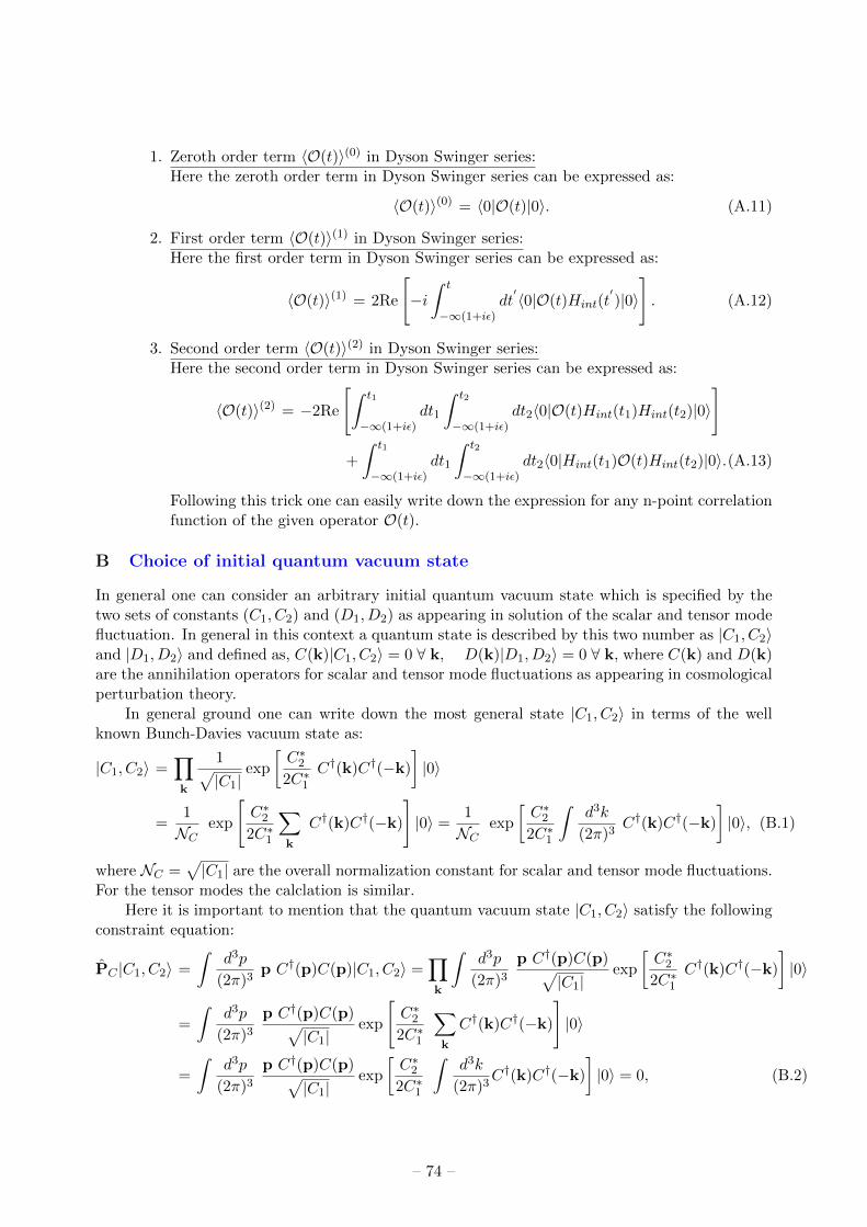
1. Zeroth order term 〈O(t)〉(0) in Dyson Swinger series:Here the zeroth order term in Dyson Swinger series can be expressed as:

〈O(t)〉(0) = 〈0|O(t)|0〉. (A.11)

2. First order term 〈O(t)〉(1) in Dyson Swinger series:Here the first order term in Dyson Swinger series can be expressed as:

〈O(t)〉(1) = 2Re

[−i∫ t

−∞(1+iε)dt′〈0|O(t)Hint(t

′)|0〉

]. (A.12)

3. Second order term 〈O(t)〉(2) in Dyson Swinger series:Here the second order term in Dyson Swinger series can be expressed as:

〈O(t)〉(2) = −2Re

[∫ t1

−∞(1+iε)dt1

∫ t2

−∞(1+iε)dt2〈0|O(t)Hint(t1)Hint(t2)|0〉

]

+

∫ t1

−∞(1+iε)dt1

∫ t2

−∞(1+iε)dt2〈0|Hint(t1)O(t)Hint(t2)|0〉.(A.13)

Following this trick one can easily write down the expression for any n-point correlationfunction of the given operator O(t).

B Choice of initial quantum vacuum state

In general one can consider an arbitrary initial quantum vacuum state which is specified by thetwo sets of constants (C1, C2) and (D1, D2) as appearing in solution of the scalar and tensor modefluctuation. In general in this context a quantum state is described by this two number as |C1, C2〉and |D1, D2〉 and defined as, C(k)|C1, C2〉 = 0 ∀ k, D(k)|D1, D2〉 = 0 ∀ k, where C(k) and D(k)are the annihilation operators for scalar and tensor mode fluctuations as appearing in cosmologicalperturbation theory.

In general ground one can write down the most general state |C1, C2〉 in terms of the wellknown Bunch-Davies vacuum state as:

|C1, C2〉 =∏k

1√|C1|

exp

[C∗22C∗1

C†(k)C†(−k)

]|0〉

=1

NCexp

[C∗22C∗1

∑k

C†(k)C†(−k)

]|0〉 =

1

NCexp

[C∗22C∗1

∫d3k

(2π)3C†(k)C†(−k)

]|0〉, (B.1)

where NC =√|C1| are the overall normalization constant for scalar and tensor mode fluctuations.

For the tensor modes the calclation is similar.Here it is important to mention that the quantum vacuum state |C1, C2〉 satisfy the following

constraint equation:

PC |C1, C2〉 =

∫d3p

(2π)3p C†(p)C(p)|C1, C2〉 =

∏k

∫d3p

(2π)3

p C†(p)C(p)√|C1|

exp

[C∗22C∗1

C†(k)C†(−k)

]|0〉

=

∫d3p

(2π)3

p C†(p)C(p)√|C1|

exp

[C∗22C∗1

∑k

C†(k)C†(−k)

]|0〉

=

∫d3p

(2π)3

p C†(p)C(p)√|C1|

exp

[C∗22C∗1

∫d3k

(2π)3C†(k)C†(−k)

]|0〉 = 0, (B.2)

– 74 –

which is true for the quantum vacuum state |D1, D2〉 for tensor modes also. Since scalar modesare exactly similar to tensor modes we will not speak about tensor modes in the next part.

Additionally, here it is important to note that, the annihilation and creation operators forBunch-Davies vacuum (a(k), a†(k)) and the arbitrary quantum vacumm |C1, C2〉 state (C(k), C†(k))are connected via the following sets of Bogoliubov transformations:

C(k) = C∗1 a(k)− C∗2 a†(−k), (B.3)

a(k) = C1 C(k) + C∗2 C†(−k). (B.4)

1. Bunch-Davies vacuum:Bunch-Davies vacuum is specified by fixing the coefficients to, C1 = 1 = D1, C2 = 0 = D2,in the solution of the scalar and tensor mode fluctuation as derived earlier. In this case thequantum vacuum state |0〉 is defined as the state that gets annihilated by the annihilationoperator, as given by, a(k)|0〉 = 0 ∀ k. Here the creation and annihilation operators a(k)and a†(k) satisfy the following canonical commutation relations:[

a(k), a(k′)]

= 0,[a†(k), a†(k

′)]

= 0,[a(k), a†(k

′)]

= (2π)3δ(3)(k + k′). (B.5)

2. α, β vacuum:

α, β vacuum is specified by fixing the coefficients to, C1 = coshα = D1, C2 = eiβ sinhα =D2, in the solution of the scalar and tensor mode fluctuation as derived earlier. In thiscase the quantum vacuum state |α, β〉 is defined as the state that gets annihilated by theannihilation operator, as given by, b(k)|α, β〉 = 0 ∀ k. Here the creation and annihilationoperators b(k) and b†(k) satisfy the following canonical commutation relations:[

b(k), b(k′)]

= 0,[b†(k), b†(k

′)]

= 0,[b(k), b†(k

′)]

= (2π)3δ(3)(k + k′). (B.6)

Here one can write the Bunch Davies vacuum state |0〉 as a special class of |α, β〉 vacuumstate. Also using Bogoliubov transformation one can write down |α, β〉 vacuum state interms of the Bunch Davies vacuum state |0〉, as given by:

|α, β〉 =∏k

1√| coshα|

exp

[− i

2e−iβ tanhα a†(k)a†(−k)

]|0〉

=1

Nexp

[− i

2e−iβ tanhα

∑k

a†(k)a†(−k)

]|0〉

=1

Nexp

[− i

2e−iβ tanhα

∫d3k

(2π)3a†(k)a†(−k)

]|0〉, (B.7)

where N =√| coshα| is the overall normalization constant. Here it is important to mention

that the |α, β〉 vacuum state satisfy the following constraint equation:

P|α, β〉 =

∫d3p

(2π)3p a†(p)a(p)|α, β〉

=∏k

∫d3p

(2π)3

p a†(p)a(p)√| coshα|

exp

[− i

2e−iβ tanhα a†(k)a†(−k)

]|0〉

=

∫d3p

(2π)3

p a†(p)a(p)√| coshα|

exp

[− i

2e−iβ tanhα

∑k

a†(k)a†(−k)

]|0〉

=

∫d3p

(2π)3

p a†(p)a(p)√| coshα|

exp

[− i

2e−iβ tanhα

∫d3k

(2π)3a†(k)a†(−k)

]|0〉 = 0,(B.8)

– 75 –

Additionally, here it is important to note that, the creation and annihilation operators forBunch-Davies vacuum and |α, β〉 vacuum state are connected via the following sets of Bo-goliubov transformations:

b(k) = coshα a(k) + i e−iβ sinhα a†(−k), (B.9)

a(k) = coshα b(k)− i e−iβ sinhα b†(−k). (B.10)

C Useful integrals as appearing in scalar three point function

All the useful integrals appearing in the scalar three point function are appended bellow:

1.

∫ 0

−∞dη η2 e±iKcSη = ∓ 2

iK3c3S

, (C.1)

2.

∫ 0

−∞dη η2 e∓i(2ka−K)cSη = ± 2

i(2ka −K)3c3S

, (C.2)

3.

∫ ηf=0

ηi=−∞dη (1∓ ikbcSη)(1∓ ikccSη) e±iKcSη =

1

iK3cS

[K2 + 2kbkc +K(K − ka)

], (C.3)

4.

∫ 0

−∞dη (1− ikbcSη)(1− ikccSη) ei(K−2ka)cSη = −

∫ 0

−∞dη (1 + ikbcSη)(1 + ikccSη) e−i(K−2ka)cSη

= − 1

i(2ka −K)3cS

[K2 + 2kbkc +K(K − 5ka)− 2(K − ka)ka + 4k2

a

], (C.4)

5.

∫ 0

−∞dη (1− ikbcSη)(1∓ ikccSη) ei(K−2kb)cSη = −

∫ 0

−∞dη (1∓ ikbcSη)(1± ikccSη) e∓i(K−2kb)cSη

= − 1

i(2kb −K)3cS

[K2 − 4kbkc +K(kc − 5kb) + 6k2

b

], (C.5)

6.

∫ 0

−∞dη (1∓ ikacSη) e±iKcSη = ± 1

iK2cS(K + ka), (C.6)

7.

∫ 0

−∞dη (1± ikacSη) e±i(K−2ka)cSη = ± (K − 3ka)

i(2ka −K)2cS, (C.7)

8.

∫ 0

−∞dη (1∓ ikacSη) e±i(K−2kb)cSη = ±(K + ka − 2kb)

i(2kb −K)2cS, (C.8)

9.

∫ 0

−∞dη (1− ikacSη)(1− ikccSη) ei(K−2kb)cSη

= − 1

i(2kb −K)3cS[(K − 2kb)(K + ka − 2kb) + (K + 2ka − 2kb)kc] . (C.9)

References

[1] A. Pich, “Effective field theory: Course,” arXiv:hep-ph/9806303.

[2] C. P. Burgess, “Introduction to Effective Field Theory,” Ann. Rev. Nucl. Part. Sci. 57 (2007) 329[hep-th/0701053].

[3] R. Shankar, “Effective field theory in condensed matter physics,” In *Boston 1996, Conceptualfoundations of quantum field theory* 47-55 [cond-mat/9703210].

[4] J. F. Donoghue, “Introduction to the effective field theory description of gravity,” arXiv:gr-qc/9512024.

– 76 –

[5] J. F. Donoghue, “The effective field theory treatment of quantum gravity,” AIP Conf. Proc. 1483 (2012)73 [arXiv:1209.3511 [gr-qc]].

[6] C. Cheung, P. Creminelli, A. L. Fitzpatrick, J. Kaplan and L. Senatore, “The Effective Field Theory ofInflation,” JHEP 0803 (2008) 014 [arXiv:0709.0293 [hep-th]].

[7] S. Weinberg, “Effective Field Theory for Inflation,” Phys. Rev. D 77 (2008) 123541 [arXiv:0804.4291[hep-th]].

[8] J. T. Giblin, E. Nesbit, O. Ozsoy, G. Sengor and S. Watson, “Toward an Effective Field Theory Approach toReheating,” arXiv:1701.01455 [hep-th].

[9] O. zsoy, G. Sengor, K. Sinha and S. Watson, “A Model Independent Approach to (p)Reheating,”arXiv:1507.06651 [hep-th].

[10] C. P. Burgess, “Intro to Effective Field Theories and Inflation,” arXiv:1711.10592 [hep-th].

[11] D. Baumann and L. McAllister, “Inflation and String Theory,” arXiv:1404.2601 [hep-th].

[12] D. Baumann, “Inflation,” arXiv:0907.5424 [hep-th].

[13] S. Choudhury, “Field Theoretic Approaches To Early Universe,” arXiv:1603.08306 [hep-th].

[14] S. Choudhury and A. Mazumdar, “An accurate bound on tensor-to-scalar ratio and the scale of inflation,”Nucl. Phys. B 882 (2014) 386 [arXiv:1306.4496 [hep-ph]].

[15] S. Choudhury, “Can Effective Field Theory of inflation generate large tensor-to-scalar ratio withinRandallSundrum single braneworld?,” Nucl. Phys. B 894 (2015) 29 [arXiv:1406.7618 [hep-th]].

[16] L. V. Delacretaz, V. Gorbenko and L. Senatore, “The Supersymmetric Effective Field Theory of Inflation,”JHEP 1703 (2017) 063 [arXiv:1610.04227 [hep-th]].

[17] L. V. Delacretaz, T. Noumi and L. Senatore, “Boost Breaking in the EFT of Inflation,” JCAP 1702(2017) no.02, 034 [arXiv:1512.04100 [hep-th]].

[18] D. Lopez Nacir, R. A. Porto, L. Senatore and M. Zaldarriaga, “Dissipative effects in the Effective FieldTheory of Inflation,” JHEP 1201 (2012) 075 [arXiv:1109.4192 [hep-th]].

[19] A. Naskar, S. Choudhury, A. Banerjee and S. Pal, “Inflation to Structures: EFT all the way,”arXiv:1706.08051 [astro-ph.CO].

[20] L. Senatore and M. Zaldarriaga, “The Effective Field Theory of Multifield Inflation,” JHEP 1204 (2012)024 [arXiv:1009.2093 [hep-th]].

[21] L. Senatore, K. M. Smith and M. Zaldarriaga, “Non-Gaussianities in Single Field Inflation and theirOptimal Limits from the WMAP 5-year Data,” JCAP 1001 (2010) 028 [arXiv:0905.3746 [astro-ph.CO]].

[22] S. R. Behbahani, A. Dymarsky, M. Mirbabayi and L. Senatore, “(Small) Resonant non-Gaussianities:Signatures of a Discrete Shift Symmetry in the Effective Field Theory of Inflation,” JCAP 1212 (2012) 036[arXiv:1111.3373 [hep-th]].

[23] C. Cheung, A. L. Fitzpatrick, J. Kaplan and L. Senatore, “On the consistency relation of the 3-pointfunction in single field inflation,” JCAP 0802 (2008) 021 [arXiv:0709.0295 [hep-th]].

[24] D. Baumann, D. Green, H. Lee and R. A. Porto, “Signs of Analyticity in Single-Field Inflation,” Phys.Rev. D 93 (2016) no.2, 023523 [arXiv:1502.07304 [hep-th]].

[25] V. Assassi, D. Baumann, D. Green and L. McAllister, “Planck-Suppressed Operators,” JCAP 1401(2014) 033 [arXiv:1304.5226 [hep-th]].

[26] S. Dubovsky, L. Hui, A. Nicolis and D. T. Son, Effective field theory for hydrodynamics: thermodynamics,and the derivative expansion, Phys. Rev. D 85 (2012) 085029 [arXiv:1107.0731 [hep-th]].

[27] M. Crossley, P. Glorioso and H. Liu, “Effective field theory of dissipative fluids,” JHEP 1709 (2017) 095[arXiv:1511.03646 [hep-th]].

[28] H. Ruegg and M. Ruiz-Altaba, “The Stueckelberg field,” Int. J. Mod. Phys. A 19 (2004) 3265[hep-th/0304245].

– 77 –

[29] C. Grosse-Knetter and R. Kogerler, “Unitary gauge, Stuckelberg formalism and gauge invariant models foreffective lagrangians,” Phys. Rev. D 48 (1993) 2865 [hep-ph/9212268].

[30] J. M. Maldacena, “Non-Gaussian features of primordial fluctuations in single field inflationary models,”JHEP 0305 (2003) 013 [astro-ph/0210603].

[31] P. A. R. Ade et al. [Planck Collaboration], “Planck 2015 results. XX. Constraints on inflation,” Astron.Astrophys. 594 (2016) A20 [arXiv:1502.02114 [astro-ph.CO]].

[32] A. Shukla, S. P. Trivedi and V. Vishal, “Symmetry constraints in inflation, α-vacua, and the three pointfunction,” JHEP 1612 (2016) 102 [arXiv:1607.08636 [hep-th]].

[33] S. Choudhury, “COSMOS-e′- soft Higgsotic attractors,” Eur. Phys. J. C 77 (2017) no.7, 469[arXiv:1703.01750 [hep-th]].

[34] S. Choudhury, “Reconstructing inflationary paradigm within Effective Field Theory framework,” Phys.Dark Univ. 11 (2016) 16 [arXiv:1508.00269 [astro-ph.CO]].

[35] S. Choudhury, B. K. Pal, B. Basu and P. Bandyopadhyay, “Quantum Gravity Effect in Torsion DrivenInflation and CP violation,” JHEP 1510 (2015) 194 [arXiv:1409.6036 [hep-th]].

[36] S. Choudhury, A. Mazumdar and S. Pal, “Low & High scale MSSM inflation, gravitational waves andconstraints from Planck,” JCAP 1307 (2013) 041 [arXiv:1305.6398 [hep-ph]].

[37] S. Choudhury, T. Chakraborty and S. Pal, “Higgs inflation from new Khler potential,” Nucl. Phys. B 880(2014) 155 [arXiv:1305.0981 [hep-th]].

[38] S. Choudhury and S. Pal, “Fourth level MSSM inflation from new flat directions,” JCAP 1204 (2012)018 [arXiv:1111.3441 [hep-ph]].

[39] S. Choudhury and S. Pal, “Brane inflation in background supergravity,” Phys. Rev. D 85 (2012) 043529[arXiv:1102.4206 [hep-th]].

[40] S. Choudhury and S. Pal, “Brane inflation: A field theory approach in background supergravity,” J. Phys.Conf. Ser. 405 (2012) 012009 [arXiv:1209.5883 [hep-th]].

[41] S. Choudhury and S. Pal, “Reheating and leptogenesis in a SUGRA inspired brane inflation,” Nucl. Phys.B 857 (2012) 85 [arXiv:1108.5676 [hep-ph]].

[42] D. Baumann and D. Green, “A Field Range Bound for General Single-Field Inflation,” JCAP 1205 (2012)017 [arXiv:1111.3040 [hep-th]].

[43] X. Chen, M. x. Huang, S. Kachru and G. Shiu, “Observational signatures and non-Gaussianities of generalsingle field inflation,” JCAP 0701 (2007) 002 [hep-th/0605045].

[44] M. Alishahiha, E. Silverstein and D. Tong, “DBI in the sky,” Phys. Rev. D 70 (2004) 123505[hep-th/0404084].

[45] S. Choudhury and S. Pal, “Primordial non-Gaussian features from DBI Galileon inflation,” Eur. Phys. J.C 75 (2015) no.6, 241 [arXiv:1210.4478 [hep-th]].

[46] S. Choudhury and S. Pal, “DBI Galileon inflation in background SUGRA,” Nucl. Phys. B 874 (2013) 85[arXiv:1208.4433 [hep-th]].

[47] S. Choudhury, A. Mazumdar and E. Pukartas, “Constraining N = 1 supergravity inflationary frameworkwith non-minimal Khler operators,” JHEP 1404 (2014) 077 [arXiv:1402.1227 [hep-th]].

[48] S. Choudhury, “Constraining N = 1 supergravity inflation with non-minimal Kaehler operators using δNformalism,” JHEP 1404 (2014) 105 [arXiv:1402.1251 [hep-th]].

[49] S. Choudhury and S. Panda, “COSMOS-e-GTachyon from string theory,” Eur. Phys. J. C 76 (2016)no.5, 278 [arXiv:1511.05734 [hep-th]].

[50] A. Bhattacharjee, A. Deshamukhya and S. Panda, “A note on low energy effective theory ofchromo-natural inflation in the light of BICEP2 results,” Mod. Phys. Lett. A 30 (2015) no.11, 1550040[arXiv:1406.5858 [astro-ph.CO]].

– 78 –

[51] P. Chingangbam, S. Panda and A. Deshamukhya, “Non-minimally coupled tachyonic inflation in warpedstring background,” JHEP 0502 (2005) 052 [hep-th/0411210].

[52] A. Mazumdar, S. Panda and A. Perez-Lorenzana, “Assisted inflation via tachyon condensation,” Nucl.Phys. B 614 (2001) 101 [hep-ph/0107058].

[53] D. Choudhury, D. Ghoshal, D. P. Jatkar and S. Panda, “Hybrid inflation and brane - anti-brane system,”JCAP 0307 (2003) 009 [hep-th/0305104].

[54] D. Choudhury, D. Ghoshal, D. P. Jatkar and S. Panda, “On the cosmological relevance of the tachyon,”Phys. Lett. B 544 (2002) 231 [hep-th/0204204].

[55] S. Panda, M. Sami and S. Tsujikawa, “Inflation and dark energy arising from geometrical tachyons,”Phys. Rev. D 73 (2006) 023515 [hep-th/0510112].

[56] D. Pirtskhalava, L. Santoni, E. Trincherini and F. Vernizzi, “Large Non-Gaussianity in Slow-Roll Inflation,”JHEP 1604 (2016) 117 [arXiv:1506.06750 [hep-th]].

[57] “Nonabelian gauge theories,” https://www.nikhef.nl/ t45/ftip/Ch12.pdf.

[58] L. Senatore and M. Zaldarriaga, “A Naturally Large Four-Point Function in Single Field Inflation,” JCAP1101 (2011) 003 [arXiv:1004.1201 [hep-th]].

[59] S. Shandera, N. Agarwal and A. Kamal, “A cosmological open quantum system,” arXiv:1708.00493[hep-th].

[60] L. M. Sieberer, M. Buchhold and S. Diehl, “Keldysh Field Theory for Driven Open Quantum Systems,”Rept. Prog. Phys. 79 (2016) no.9, 096001 [arXiv:1512.00637 [cond-mat.quant-gas]].

[61] A. Baidya, C. Jana, R. Loganayagam and A. Rudra, “Renormalization in open quantum field theory. PartI. Scalar field theory,” JHEP 1711 (2017) 204 [arXiv:1704.08335 [hep-th]].

[62] A. K. Das, S. Panda and J. R. L. Santos, “A path integral approach to the Langevin equation,” Int. J.Mod. Phys. A 30 (2015) no.07, 1550028 [arXiv:1411.0256 [hep-th]].

[63] M. A. Amin and D. Baumann, “From Wires to Cosmology,” JCAP 1602 (2016) no.02, 045[arXiv:1512.02637 [astro-ph.CO]].

[64] M. A. Amin, M. A. G. Garcia, H. Y. Xie and O. Wen, “Multifield Stochastic Particle Production: Beyonda Maximum Entropy Ansatz,” JCAP 1709 (2017) no.09, 015 [arXiv:1706.02319 [astro-ph.CO]].

[65] B. L. Hu and S. Sinha, “A Fluctuation - dissipation relation for semiclassical cosmology,” Phys. Rev. D51 (1995) 1587 [gr-qc/9403054].

[66] P. Carrilho and R. H. Ribeiro, “Quantum quenches during inflation,” Phys. Rev. D 95 (2017) no.4,043516 [arXiv:1612.00035 [hep-th]].

– 79 –