Co-Clustering of Image Segments Using Convex Optimization Applied to EMNeuronal Reconstruction

Shiv N. VitaladevuniJanelia Farm Research Campus,

Howard Hughes Medical Institutevitaladevunis@janelia.hhmi.org

Ronen BasriDept. of Computer Science and Applied Math,

Weizmann Institute of Science

Abstract

This paper addresses the problem of jointly clusteringtwo segmentations of closely correlated images. We fo-cus in particular on the application of reconstructing neu-ronal structures in over-segmented electron microscopy im-ages. We formulate the problem of co-clustering as aquadratic semi-assignment problem and investigate convexrelaxations using semidefinite and linear programming. Wefurther introduce a linear programming method with man-ageable number of constraints and present an approach forlearning the cost function. Our method increases computa-tional efficiency by orders of magnitude while maintainingaccuracy, automatically finds the optimal number of clus-ters, and empirically tends to produce binary assignmentsolutions. We illustrate our approach in simulations and inexperiments with real EM data.

1. Introduction

We address the problem of jointly clustering two seg-mentations of an image or two closely correlated images,so as to ensure good matching between the clusters in thetwo segmentations. We pose this as an optimization prob-lem and apply our approach to neuronal reconstruction fromelectron microscopy (EM) images.

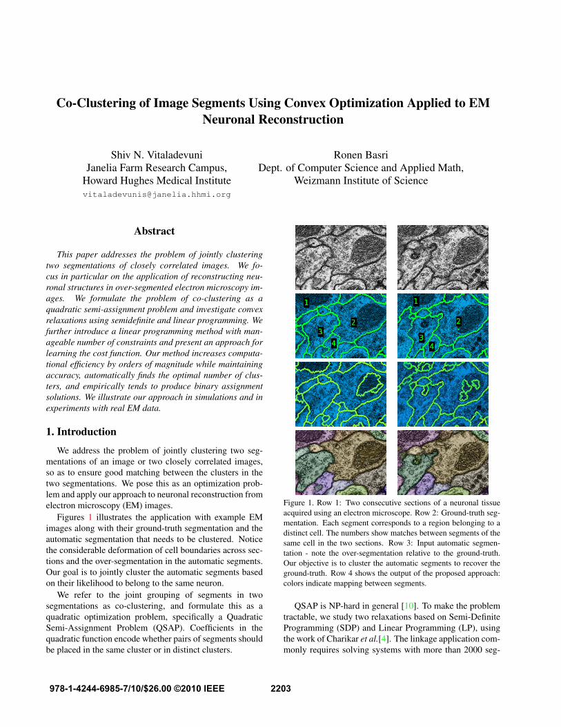
Figures 1 illustrates the application with example EMimages along with their ground-truth segmentation and theautomatic segmentation that needs to be clustered. Noticethe considerable deformation of cell boundaries across sec-tions and the over-segmentation in the automatic segments.Our goal is to jointly cluster the automatic segments basedon their likelihood to belong to the same neuron.

We refer to the joint grouping of segments in twosegmentations as co-clustering, and formulate this as aquadratic optimization problem, specifically a QuadraticSemi-Assignment Problem (QSAP). Coefficients in thequadratic function encode whether pairs of segments shouldbe placed in the same cluster or in distinct clusters.

Figure 1. Row 1: Two consecutive sections of a neuronal tissueacquired using an electron microscope. Row 2: Ground-truth seg-mentation. Each segment corresponds to a region belonging to adistinct cell. The numbers show matches between segments of thesame cell in the two sections. Row 3: Input automatic segmen-tation - note the over-segmentation relative to the ground-truth.Our objective is to cluster the automatic segments to recover theground-truth. Row 4 shows the output of the proposed approach:colors indicate mapping between segments.

QSAP is NP-hard in general [10]. To make the problemtractable, we study two relaxations based on Semi-DefiniteProgramming (SDP) and Linear Programming (LP), usingthe work of Charikar et al.[4]. The linkage application com-monly requires solving systems with more than 2000 seg-

2203978-1-4244-6985-7/10/$26.00 ©2010 IEEE

ments; we found the SDP solution to be impractical forsuch large systems. The LP formulation proposed in [4]also proved to be impractical for large systems. This for-mulation involves enforcing triangular inequalities, requir-ing therefore O(n3) constraints, where n is the number ofsegments. This results in billions of inequalities for typicalsystems. We address this by enforcing only the local metricconstraints, bounding the number of constraints to O(n2).We found that this greatly reduces the time-complexity ofthe optimization without significantly affecting the accu-racy.

We present an approach to learning the coefficients ofthe optimization function using a boosted classifier trainedto minimize the Rand index error of the classification. Thisopens up the possibility of applying the results to other co-clustering problems in vision.

Computing globally optimal binary solutions from thereal-valued solutions obtained from the SDP and LP isNP -hard. We present empirical results of LP’s integrality, andtheoretical discussions about the relation of the integralityof our LP solution to studies in optimization theory.

We compare the performance of the LP formulation withthe SDP version, normalized cuts, and connected compo-nents with learned cost function. Experiments indicate theutility of the proposed approach.

2. Co-clustering problemLet Ω ⊂ <2 denote a discrete 2D domain of points (pix-

els), and let P and Q denote two segmentations of Ω; P =piNi=1 and Q = qiMi=1 are two non-overlapping parti-tions of Ω (pi∩pj = ∅, qk ∩ ql = ∅ and ∪ipi = ∪jqj = Ω).Such segmentations can be obtained by applying two differ-ent segmentation algorithms to an image or by segmentingtwo closely correlated images. Our objective is to clusterthe segments in P and Q simultaneously, so as to obtain agood match between clusters in P and Q. We further as-sume that P and Q are over-segmentations of Ω, and hencewe do not need to consider splitting a segment to achieve agood match.

Let C be the set of clusters, such that each cluster C ∈ Cis a subset of P ∪Q. We associate a cost with C defined as

H(C) =∑C∈C

∑r,r′∈C

F (r, r′) (1)

with F (r, r′) ∈ R and expressH(C) as a quadratic functionas follows. Let xC ∈ 0, 1N denote a vector indicatingwhich of the segments in P belongs to cluster C. Similarly,let yC ∈ 0, 1M be the indicator vector for segments in Qthat belong toC. Let zC ∈ 0, 1N+M be a vector obtainedby concatenating xC and yC (i.e., zC = [xT

C yTC ]T ). H(C)

is then expressed by a general quadratic function on pairsof elements in the clusters, as H(C) =

∑C∈C zT

C F zC .

Our objective is to compute the clustering that minimizesthe cost H(C), stated as

Min : H(C) =∑C∈C

zTC F zC

s.t. zC ∈ 0, 1N+M and∑C

(zC)i = 1 ∀i, (2)

where the constraints ensure that each segment in P and Qparticipates in exactly one cluster. Note that while we focushere on co-clustering, the formulation and its solutions areapplicable to the general problem of clustering as well.

When the number of clusters |C| is known, the opti-mization (2) is equivalent to finding the minimal k-cut ina weighted graph G with the edge weight matrix set to −F .Here, each cluster corresponds to a component in G andk = |C| is the known number of clusters. For the equiv-alence, notice that when the edge matrix is set to −F , Mink-cut minimizes

∑C(1−zC)T (−F )zC , which is the same

as minimizing zTCFzC , as all the vertices in the graph are

forced to belong to exactly one component in G.While the problem of finding the minimal k-cut with

non-negative weights and with a fixed number of clustershas a polynomial solution (with complexity O(nk2

)), theproblem of finding the minimal cut with negative weights orwith an unknown number of clusters is NP-hard [7]. Moregenerally, this problem can be viewed as a Quadratic Semi-Assignment Problem (QSAP) which is also NP-hard [10].The focus of our work is to construct tractable relaxationsthat exhibit good empirical performance in the EM recon-struction application. An SDP relaxation, along with an LPrelaxation based on Charikar et al. [4], form the startingpoint for our work.

Image segmentation has been addressed with graphtheoretic algorithms, most notably with Shi and Malik’sNormalized-cuts [14]. Yu and Shi modified N-cuts to han-dle negative weights and used their modification to model“pop-out” in perceptual grouping [17]. Cosegmentation ofan object occuring in two images has been studied in [12]and [11].

3. Convex Relaxations

DeBie and Cristianini presented a fast SDP relaxationof N-cuts and Max-cut [2]. Also, Xing and Jordan studySDP relaxation of k-Ncuts [16]. QSAP is a special caseof Quadratic Assignment Problem (QAP). Many problems,such as the traveling salesman problem and graph partition-ing, can be formulated as QAP, which is also NP -hard anddifficult to even approximate [10]. Schellewald et al. studyconvex relaxations of QAP for feature matching in [13]. Aclosely related work of Kumar et al. deals with convexrelaxations of quadratic optimization problems [9].

2204

3.1. Semi-Definite Program (SDP) relaxation

Let Z = [z1 . . . z|C|], andR = ZZT , Z is (N+M)×|C|andR is (N+M)×(N+M). Here,R is akin to the clusterco-occurrence matrix; it is 1 when two segments belong tothe same cluster and 0 otherwise. In the spirit of Goemansand Williamson’s approximation algorithm for the maxi-mum cut [6] we relax R to obtain real-valued entries andrestate (2) as a Semi-Definite Program (SDP):

Min : Trace(FTR)s.t. : R 0, Rij ∈ [0, 1] ∀i, j, and Rii = 1 ∀i. (3)

(Note that we assume that F has negative weights, or elsethe identity matrix would form a trivial solution.) The re-laxed problem is convex for arbitrary F , and it is possible tocompute a globally optimal real-valued solution. Anotheradvantage is that the optimization does not require aprioriknowledge of the number of clusters.

It is generally NP-hard to convert the obtained real-valued solution to a globally optimal binary solution. Acommon heuristic to obtaining a binary solution [6] is tofactorize the optimal R to QQT using Cholesky decompo-sition and then convertQ to binary values, e.g., by assigning1 in each row to the coordinate with the maximal value inthat row. We refer to this post-processing approach by SDP-fact. Another possibility is to consider R as an adjacencymatrix of a weighted undirected graph. Clustering is thencomputed by finding connected components in a sub-graphobtained by considering edges with weights above a thresh-old. This post-processing approach is referred to as SDP-thresh. We pursued both approaches in our experiments.

We observed that current implementations of SDPsolvers, including SDPT3 [15], SeDuMi and SDPLR [3],have difficulty solving problems constructed for the EM ap-plication when the number of variables was in the 1000’s,i.e. N + M ≈ 2000. The theoretical computationalcomplexity of general SDP solvers is high, growing asO((]var)2(size SDP)2.5) [2]. In practice, the solvers im-prove their efficiency by exploiting the structure of specificproblems. However, current solvers find our applicationchallenging.

3.2. Linear Program (LP) relaxation

Given the practical issues with SDP, we use a LinearProgramming relaxation based on [4]. Notice that R is amatrix of inner products between vectors, Rij = vi · vj

where the vectors vi = [ZiC ]C∈C populate the rows of Zand indicate for each segment i its cluster association. Letdij = 1√

2‖vi − vj‖2, where

√2dij denotes the `2 distance

between vi and vj in the cluster space. Since we require‖vi‖ = 1 for all i, we have

d2ij =

12(‖vi‖22 + ‖vj‖22 − 2vi · vj

)= 1−Rij . (4)

Let D = [dij ]; our objective then is to maximizeTrace(FTD). We relax the entries in D from being `2 dis-tances to being a metric, i.e., nonnegative, symmetric andfollow the triangular inequality. This constraint is validbecause a clustering induces an equivalence relation, andhence by transitivity dik = dkj = 0 implies that alsodij = 0 while if dik +dkj ∈ 1, 2 the triangular inequalityis satisfied trivially. The LP formulation then is

Max :∑

i,j Fijdij

s.t. : 0 ≤ dij ≤ 1 , dij = dji ∀i, j, dii = 0 ∀i,and dij ≤ dik + dkj ∀i, j, k. (5)

After optimizing this cost function we post-process the so-lutions by thresholding the matrix D and considering theconnected components obtained by eliminating edges withweights exceeding a specified threshold.

Although the metric constraints used with the LP for-mulation seem to be weaker than the SDP formulation, wewill show empirically cases in which the LP optimizationperforms better than the SDP. Note that while in generalSDP problems may be expressed as linear programs withinfinite number of constraints [8], this proposed LP formu-lation has only a finite number of constraints. However, thenumber of triangular inequalities in the LP grows as O(n3)where n is the number of variables. For a typical EM co-clustering problem with 2000 variables, we will have morethan 3× 8× 109 inequalities! We found this to be imprac-tical – we tested this using lp solve, a state-of-the-art opensource solver. We therefore seek to reduce the number ofconstraints while maintaining empirical performance.

3.3. LP-R - LP with local metric constraints

We further relax our LP formulation by constraining thedistances in D to satisfy the triangular inequality only lo-cally. Consider a graph GP consisting of nodes correspond-ing to segments, pi ∈ P , and edges connecting spatiallyadjacent segments. Similarly, a graph GQ is defined for seg-mentation Q. Let G be a graph constructed by combiningGP and GQ and adding edges between overlapping segmentpairs pi ∈ P and qj ∈ Q. The distances in D are con-strained to be locally metric within all cliques in G. LetE = eij be the set of edges in G. The reduced LP ver-sion, referred to as LP-R, is

Max :∑

i,j Fijdij

s.t. 0 ≤ dij ≤ 1 , dij = dji ∀i, j, dii = 0 ∀i, anddij ≤ dik + dkj ∀eij , eik and ejk ∈ E. (6)

The number of constraints in LP-R is 3 times the num-ber of 3-cliques in G. Let us first count the number of 3-cliques within GP and GQ separately. The segments in Pand Q are constrained to be connected regions in the image

2205

plane. Therefore, GP and GQ are planar graphs, and hencethe number of 3-cliques within GP is O(n), and similarlyfor GQ. For counting the 3-cliques that extend across GP

and GQ, consider without loss of generality 3-cliques withtwo nodes in GP and one in GQ. There are O(n) edges inGP , and each adjacent pair can be simultaneously adjacenttoO(n) nodes in GQ. Therefore, the number of such cliquesis bounded by O(n2). Thus, the number of inequalities inLP-R grows as O(n2). We observed empirically that thenumber of inequalities grows almost linearly with respectto the number of segments.

3.4. Non-integrality of LP solutions

Our goal in clustering is to assign exactly one cluster toevery segment from P∪Q. We therefore want our optimiza-tion to yield binary solutions. The LP formulation, however,only limits the variables to lie within the [0, 1] range and abinary solution is not guaranteed.

One way to demonstrate that an LP system achieves bi-nary solutions is to examine the vertices of the feasibilitypolytope. If all of the vertices are binary then a binaryoptimal solution must exist. To examine the vertices, con-sider the set of hyperplanes that compose the inequality con-straints in our LP system (5). Denote these hyperplanes byAd = b. Every vertex in the polytope lies at the intersec-tion of a subset of these hyperplanes. A sufficient conditionfor the vertices to be binary is if the matrix A is totally uni-modular (TUM), that is, if the determinant of every squaresubset of the rows and columns of A belongs to −1, 0, 1,and if b is integer.

Unfortunately, our constraint matrix is not totally uni-modular. The matrix A can be viewed as the node-hyperedge incidence matrix of a directed hypergraph H.The nodes in H correspond to the variables dij (columnsof A), and each row of A that corresponds to a triangularinequality constraint represents a hyperedge with one headand two tails. For example, the inequality d12 + d13 ≥ d23

forms a directed hyperedge connecting the tail nodes d12

and d13 to the head node d23. Such a hypergraph is called 2-LDH (Leontief Directed Hypergraph). Coullard and Ng [5]showed that the incidence matrix of a 2-LDH H is totallyunimodular if and only if there exists no odd pseudo-cyclein H. (A pseudo-cycle in H is a sequence of nodes whereeach node is connected to its successor in the cycle by a dis-tinct hyperedge and that contains at least one tail-tail arc.An odd pseudo-cycle is a pseudo-cycle with odd number oftail-tail arcs.) We next construct an odd pseudo-cycle anduse this construction to find a vertex with non-binary values.

Consider a system with 4 segments, denoted 1, 2, 3, and4, and denote the unknown distances between those seg-ments by dij , 1 ≤ i, j ≤ 4. Consider a vertex of the fea-sibility polytope obtained by the following subset of con-

straints:

Ad =

1 1 0 −1 0 01 0 1 0 −1 00 1 1 0 0 −10 0 0 1 0 00 0 0 0 1 00 0 0 0 0 1

d12

d13

d14

d23

d24

d34

=

000111

.

A is a sub-matrix of A with the first three rows represent-ing triangular inequalities between subsets of the six vari-ables and the last three rows representing the constraintsthat limit variables to take values ≤ 1. Indeed, the cycled12 → d13 → d14 → d12 forms a 3-pseudo-cycle (andhence the determinant of the top-left 3 × 3 sub-matrix ofA is -2) implying that A is not totally unimodular. Conse-quently these six constraints intersect at a non-binary point〈d12 = d13 = d14 = 1/2, d23 = d24 = d34 = 1〉. Infact, the matrix A contains many more odd pseudo-cyclesand hence, many vertices with rational values exist. Still,our simulations and experiments with real data demonstratethat typically we can find solutions in which many of thevariables obtain binary values.

4. Learning the cost function

Quadratic cost functions can be used to encode a vari-ety of criteria for clustering. For example, in Section 5 wedemonstrate properties of our algorithm using a cost func-tion that relies on the shape of the segments. Specifically,we construct a function that seeks clusters of segments inP and Q whose symmetric difference is minimal. Like-wise, criteria that involve intensities and texture can also beincorporated. Furthermore, for a variety of applications itmay make sense to learn the cost function from examples.In this section we describe a simple procedure for learningthe cost function from training data. This procedure is laterused in Section 6 to link regions corresponding to neuronalcells across EM sections.

Our objective is, given training data, to learn the compo-nents of F from properties of the segments in P and Q. Intraining, we assume that we are given the results of two au-tomatic segmentations P = pi and Q = qi along withthe ground-truth clustering, i.e., the desired partition of theset of segments P ∪ Q. Let Rgt denote the co-occurrencematrix for the ground-truth clustering (as in Section 3.1,Rgt

ij = 1 if segments i and j belong to the same groundtruth cluster and zero otherwise). Let R denote the co-occurrence matrix computed using a co-clustering formula-tion. To evaluate the accuracy of R we use the Rand index,which has been used extensively for evaluating clusteringand segmentation algorithms, e.g. [1]. Denote respectivelyby lgt(r) and lcc(r) the cluster assigned to a segment r inthe ground truth and in the computed co-clustering. TheRand index counts the number of false merges and splits in

2206

the computed co-clustering as follows.∑r,r′∈P∪Q

1 (lgt(r) = lgt(r′) ∧ lcc(r) 6= lcc(r′)) +

1 (lgt(r) 6= lgt(r′) ∧ lcc(r) = lcc(r′)) . (7)

where 1(.) denotes binary indicator function and ∧ is thelogical and operator. This measure can be expressed interms of the co-occurrence matrices Rgt and R as follows.

Rand(R) =∑

i,j [1−Rij ]Rgtij +

∑i,j Rij [1−Rgt

ij ]=

∑i,j [1− 2Rgt

ij ]Rij + c,

where c =∑

ij Rgtij is a constant independent of R. Com-

pare this with the SDP and LP formulations (3) and (5), ifF was defined as 1− 2Rgt, minimizing the Rand error canbe posed as a QSAP problem. We therefore seek a functionthat assigns to Fij the values −1 and +1 to pairs of to-be-linked and not-to-be-linked segments in P ∪Q respectively.

There have been numerous studies on trainable cluster-ing and segmentation algorithms. Here we use a boostedclassifier to learn the cost function for the optimization, anduse intensity histograms as features. For pairs of segmentsbelonging to the same section (p, p′ ∈ P and q, q′ ∈ Q) wecompute their histograms of intensities along their bound-ary interface. For pairs of segments that belong to adjacentsections, p ∈ P and q ∈ Q, we compute the intensity his-togram in the region of overlap (p ∩ q), and concatenate itto the histograms of the individual segments p and q. Wechose to use intensity histograms despite their simplicity asthey have been used effectively in a variety of applicationssuch as object recognition and tracking. The Gentle-Boostclassifier outputs a “soft” confidence value. As we seek torely on the information for which the classification is moreconfident we allow F to attain real values, and so we di-rectly use the values returned by the Gentle-Boost classifierto populate F . We further trade-off between false split andfalse merge errors by assigning different costs during train-ing to errors in classifying samples with ground-truth labels+1 and −1.

In the rest of the text, the co-clustering formulationscombined with boosting are referred to as B-SDP, B-LP andB-LP-R.

5. Simulation experimentsWe illustrate the co-clustering problem and the proposed

formulation through simulation experiments. The resultshighlight (a) the relative sparsity of the optimization so-lutions, (b) the similarity in the results obtained with theSDP and LP formulations, and (c) the need for caution whendefining the objective function to avoid trivial solutions.

For the simulations, we define the following problem.We are given as input two segmentations of an image thatare noisy refinements of some ground-truth segmentation.

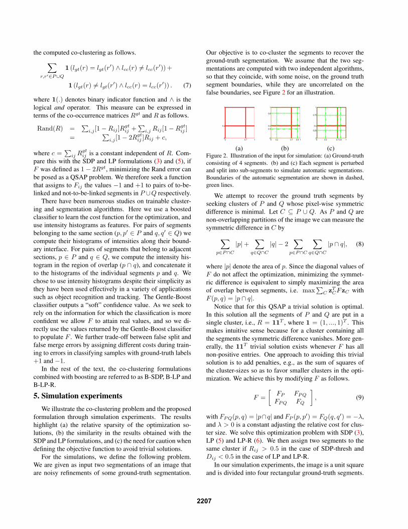
Our objective is to co-cluster the segments to recover theground-truth segmentation. We assume that the two seg-mentations are computed with two independent algorithms,so that they coincide, with some noise, on the ground truthsegment boundaries, while they are uncorrelated on thefalse boundaries, see Figure 2 for an illustration.

0 0.7 10

0.4

1

0 0.2 0.7 0.9 10

0.3

0.4

0.8

1

0 0.3 0.7 0.8 10

0.25

0.4

0.75

1

(a) (b) (c)Figure 2. Illustration of the input for simulation: (a) Ground-truthconsisting of 4 segments. (b) and (c) Each segment is perturbedand split into sub-segments to simulate automatic segmentations.Boundaries of the automatic segmentation are shown in dashed,green lines.

We attempt to recover the ground truth segments byseeking clusters of P and Q whose pixel-wise symmetricdifference is minimal. Let C ⊆ P ∪ Q. As P and Q arenon-overlapping partitions of the image we can measure thesymmetric difference in C by∑

p∈P∩C

|p|+∑

q∈Q∩C

|q| − 2∑

p∈P∩C

∑q∈Q∩C

|p ∩ q|, (8)

where |p| denote the area of p. Since the diagonal values ofF do not affect the optimization, minimizing the symmet-ric difference is equivalent to simply maximizing the areaof overlap between segments, i.e. max

∑C zT

CFzC withF (p, q) = |p ∩ q|.

Notice that for this QSAP a trivial solution is optimal.In this solution all the segments of P and Q are put in asingle cluster, i.e., R = 11T , where 1 = (1, ..., 1)T . Thismakes intuitive sense because for a cluster containing allthe segments the symmetric difference vanishes. More gen-erally, the 11T trivial solution exists whenever F has allnon-positive entries. One approach to avoiding this trivialsolution is to add penalties, e.g., as the sum of squares ofthe cluster-sizes so as to favor smaller clusters in the opti-mization. We achieve this by modifying F as follows.

F =[

FP FPQ

FPQ FQ

], (9)

with FPQ(p, q) = |p∩q| and FP (p, p′) = FQ(q, q′) = −λ,and λ > 0 is a constant adjusting the relative cost for clus-ter size. We solve this optimization problem with SDP (3),LP (5) and LP-R (6). We then assign two segments to thesame cluster if Rij > 0.5 in the case of SDP-thresh andDij < 0.5 in the case of LP and LP-R.

In our simulation experiments, the image is a unit squareand is divided into four rectangular ground-truth segments.

2207

0.02 0.04 0.06 0.08 0.1 0.12

40

50

60

70

80

Noise level

#trials with 0 Rand error

CC

SDP−thresh

SDP−fact

LP

LP−R

0.02 0.04 0.06 0.08 0.1 0.120

1

2

3

4x 10

−3

Noise level

Median area of Rand error

CC

SDP−thresh

SDP−fact

LP

LP−R

0.02 0.04 0.06 0.08 0.1 0.120

20

40

60

80

100

120

Noise levelAvg. num non−binary values

per trial

SDPLPLP−R

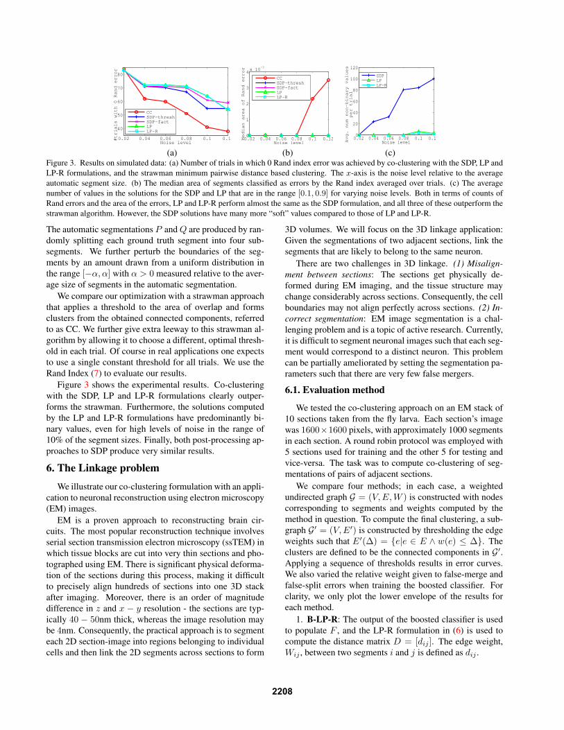
(a) (b) (c)Figure 3. Results on simulated data: (a) Number of trials in which 0 Rand index error was achieved by co-clustering with the SDP, LP andLP-R formulations, and the strawman minimum pairwise distance based clustering. The x-axis is the noise level relative to the averageautomatic segment size. (b) The median area of segments classified as errors by the Rand index averaged over trials. (c) The averagenumber of values in the solutions for the SDP and LP that are in the range [0.1, 0.9] for varying noise levels. Both in terms of counts ofRand errors and the area of the errors, LP and LP-R perform almost the same as the SDP formulation, and all three of these outperform thestrawman algorithm. However, the SDP solutions have many more “soft” values compared to those of LP and LP-R.

The automatic segmentations P andQ are produced by ran-domly splitting each ground truth segment into four sub-segments. We further perturb the boundaries of the seg-ments by an amount drawn from a uniform distribution inthe range [−α, α] with α > 0 measured relative to the aver-age size of segments in the automatic segmentation.

We compare our optimization with a strawman approachthat applies a threshold to the area of overlap and formsclusters from the obtained connected components, referredto as CC. We further give extra leeway to this strawman al-gorithm by allowing it to choose a different, optimal thresh-old in each trial. Of course in real applications one expectsto use a single constant threshold for all trials. We use theRand Index (7) to evaluate our results.

Figure 3 shows the experimental results. Co-clusteringwith the SDP, LP and LP-R formulations clearly outper-forms the strawman. Furthermore, the solutions computedby the LP and LP-R formulations have predominantly bi-nary values, even for high levels of noise in the range of10% of the segment sizes. Finally, both post-processing ap-proaches to SDP produce very similar results.

6. The Linkage problem

We illustrate our co-clustering formulation with an appli-cation to neuronal reconstruction using electron microscopy(EM) images.

EM is a proven approach to reconstructing brain cir-cuits. The most popular reconstruction technique involvesserial section transmission electron microscopy (ssTEM) inwhich tissue blocks are cut into very thin sections and pho-tographed using EM. There is significant physical deforma-tion of the sections during this process, making it difficultto precisely align hundreds of sections into one 3D stackafter imaging. Moreover, there is an order of magnitudedifference in z and x − y resolution - the sections are typ-ically 40 − 50nm thick, whereas the image resolution maybe 4nm. Consequently, the practical approach is to segmenteach 2D section-image into regions belonging to individualcells and then link the 2D segments across sections to form

3D volumes. We will focus on the 3D linkage application:Given the segmentations of two adjacent sections, link thesegments that are likely to belong to the same neuron.

There are two challenges in 3D linkage. (1) Misalign-ment between sections: The sections get physically de-formed during EM imaging, and the tissue structure maychange considerably across sections. Consequently, the cellboundaries may not align perfectly across sections. (2) In-correct segmentation: EM image segmentation is a chal-lenging problem and is a topic of active research. Currently,it is difficult to segment neuronal images such that each seg-ment would correspond to a distinct neuron. This problemcan be partially ameliorated by setting the segmentation pa-rameters such that there are very few false mergers.

6.1. Evaluation method

We tested the co-clustering approach on an EM stack of10 sections taken from the fly larva. Each section’s imagewas 1600×1600 pixels, with approximately 1000 segmentsin each section. A round robin protocol was employed with5 sections used for training and the other 5 for testing andvice-versa. The task was to compute co-clustering of seg-mentations of pairs of adjacent sections.

We compare four methods; in each case, a weightedundirected graph G = (V,E,W ) is constructed with nodescorresponding to segments and weights computed by themethod in question. To compute the final clustering, a sub-graph G′ = (V,E′) is constructed by thresholding the edgeweights such that E′(∆) = e|e ∈ E ∧ w(e) ≤ ∆. Theclusters are defined to be the connected components in G′.Applying a sequence of thresholds results in error curves.We also varied the relative weight given to false-merge andfalse-split errors when training the boosted classifier. Forclarity, we only plot the lower envelope of the results foreach method.

1. B-LP-R: The output of the boosted classifier is usedto populate F , and the LP-R formulation in (6) is used tocompute the distance matrix D = [dij ]. The edge weight,Wij , between two segments i and j is defined as dij .

2208

2.LP-R(S-Diff): LP-R is used to optimize the symmetricdifference cost function (9) with λ = 1000. The weightsWare set according to D.

3. B-Ncuts: Normalized-cuts was used to cluster thesegments with the weighted adjacency matrix defined to be−F , the output of the boosted classifier. As the original ver-sion of N-cuts was defined for non-negative weights [14],we tried the following variations: (a) B-Ncuts: ignorethe negative weights, (b) B-Norm-Ncuts: normalize theweights to the [0, 1] range, and (c) B-Neg-Ncuts: use an ex-tension of N-cuts to handle negative weights [17]. We foundB-Ncuts and B-Neg-Ncuts to be better than B-Norm-Ncuts.In case of B-Neg-Ncuts, we also tried varying the relativeweight given to positive and negative values in F . The out-put of Ncuts is a set of eigenvectors whose components de-fine the coordinates of the segments in the cluster space.We compute pairwise distance between the segments in thiscluster space and use them to define the edge-weights, Win G.

4. B-CC: Clustering by connected components. Theedge weights, W , in G are simply the output of the boostedclassifier.

0 500 1000 1500 2000 25001.5

2

2.5

3

3.5

4x 10

4

number of false merge pairs

number of false split pairs

B−LP−RB−CCB−NcutsB−Neg−NcutsLP−R (S−Diff)

0 20 40 60 80 100

200

300

400

500

600

700

800

900

1000

number of required splits

number of required mergers

B−LP−R

B−CC

B−Ncuts

B−Neg−Ncuts

LP−R (S−Diff)

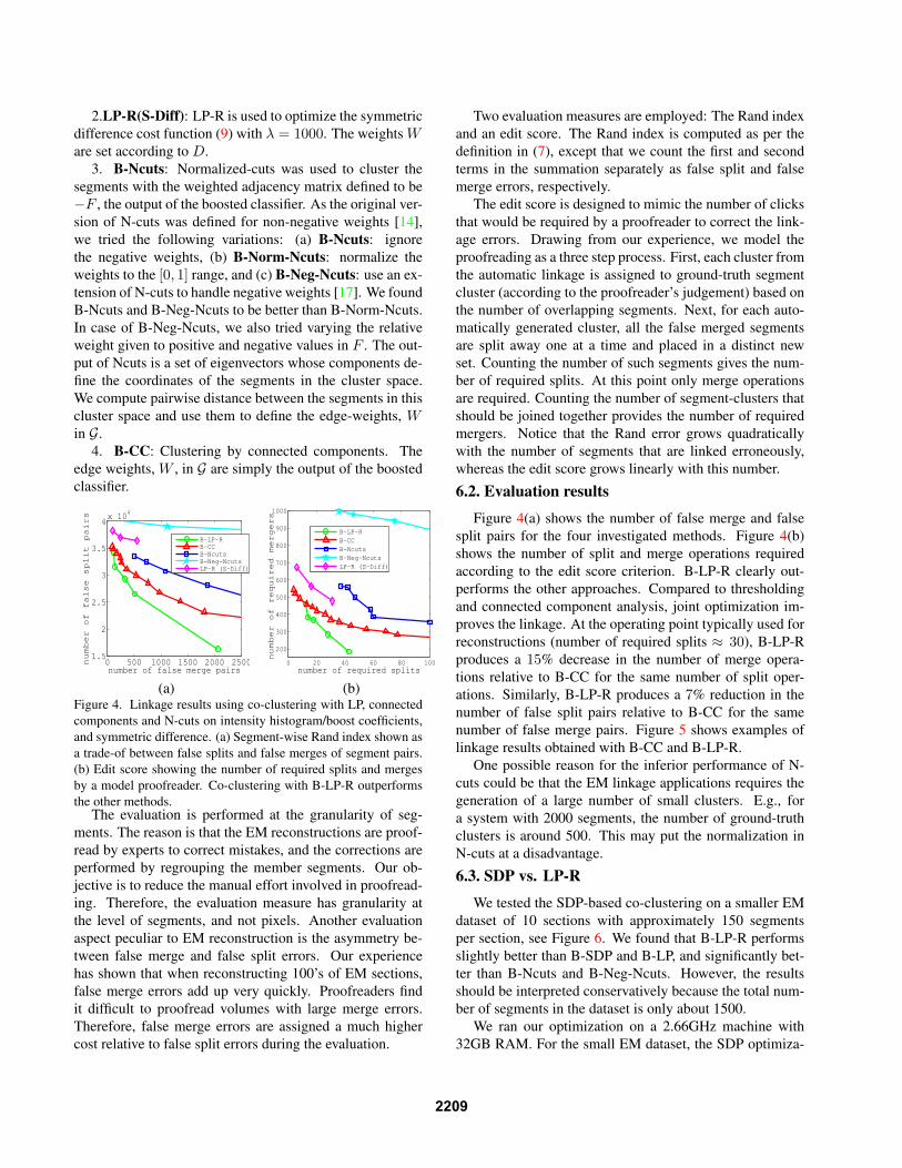
(a) (b)Figure 4. Linkage results using co-clustering with LP, connectedcomponents and N-cuts on intensity histogram/boost coefficients,and symmetric difference. (a) Segment-wise Rand index shown asa trade-of between false splits and false merges of segment pairs.(b) Edit score showing the number of required splits and mergesby a model proofreader. Co-clustering with B-LP-R outperformsthe other methods.

The evaluation is performed at the granularity of seg-ments. The reason is that the EM reconstructions are proof-read by experts to correct mistakes, and the corrections areperformed by regrouping the member segments. Our ob-jective is to reduce the manual effort involved in proofread-ing. Therefore, the evaluation measure has granularity atthe level of segments, and not pixels. Another evaluationaspect peculiar to EM reconstruction is the asymmetry be-tween false merge and false split errors. Our experiencehas shown that when reconstructing 100’s of EM sections,false merge errors add up very quickly. Proofreaders findit difficult to proofread volumes with large merge errors.Therefore, false merge errors are assigned a much highercost relative to false split errors during the evaluation.

Two evaluation measures are employed: The Rand indexand an edit score. The Rand index is computed as per thedefinition in (7), except that we count the first and secondterms in the summation separately as false split and falsemerge errors, respectively.

The edit score is designed to mimic the number of clicksthat would be required by a proofreader to correct the link-age errors. Drawing from our experience, we model theproofreading as a three step process. First, each cluster fromthe automatic linkage is assigned to ground-truth segmentcluster (according to the proofreader’s judgement) based onthe number of overlapping segments. Next, for each auto-matically generated cluster, all the false merged segmentsare split away one at a time and placed in a distinct newset. Counting the number of such segments gives the num-ber of required splits. At this point only merge operationsare required. Counting the number of segment-clusters thatshould be joined together provides the number of requiredmergers. Notice that the Rand error grows quadraticallywith the number of segments that are linked erroneously,whereas the edit score grows linearly with this number.

6.2. Evaluation results

Figure 4(a) shows the number of false merge and falsesplit pairs for the four investigated methods. Figure 4(b)shows the number of split and merge operations requiredaccording to the edit score criterion. B-LP-R clearly out-performs the other approaches. Compared to thresholdingand connected component analysis, joint optimization im-proves the linkage. At the operating point typically used forreconstructions (number of required splits ≈ 30), B-LP-Rproduces a 15% decrease in the number of merge opera-tions relative to B-CC for the same number of split oper-ations. Similarly, B-LP-R produces a 7% reduction in thenumber of false split pairs relative to B-CC for the samenumber of false merge pairs. Figure 5 shows examples oflinkage results obtained with B-CC and B-LP-R.

One possible reason for the inferior performance of N-cuts could be that the EM linkage applications requires thegeneration of a large number of small clusters. E.g., fora system with 2000 segments, the number of ground-truthclusters is around 500. This may put the normalization inN-cuts at a disadvantage.

6.3. SDP vs. LP-R

We tested the SDP-based co-clustering on a smaller EMdataset of 10 sections with approximately 150 segmentsper section, see Figure 6. We found that B-LP-R performsslightly better than B-SDP and B-LP, and significantly bet-ter than B-Ncuts and B-Neg-Ncuts. However, the resultsshould be interpreted conservatively because the total num-ber of segments in the dataset is only about 1500.

We ran our optimization on a 2.66GHz machine with32GB RAM. For the small EM dataset, the SDP optimiza-

2209

tion using SDPT3 took roughly 1800 seconds. The LP withall triangular inequalities took roughly 200 seconds, whilethe LP-R took less than 1 second. Neither SDP nor LP couldnot be used on the larger dataset with ≈1000 segment persection; only LP-R was feasible and took 5 to 7 seconds.

We found the results of LP-R to be very sparse and withfew non-binary values. For systems with F and D ap-proximately of size 1800 × 1800, the number of non-zerovalues in 1 − D was approximately 4000 (≈ 0.1%) andthe number of values in the range [0.1, 0.9] was around 60(≈ 2 × 10−3%). For the smaller EM dataset with F andD of size 150 × 150, LP-R solutions had no values in therange [0.1, 0.9]. For the same systems, SDP had around 400values (≈ 2%) in the range [0.1, 0.9].

B-C

CB

-LP-

R

section 1 section 2Figure 5. Linkage results for B-CC and B-LP-R at an operatingpoint with number of false split pairs≈ 2.9× 104, or equivalentlythe number of required mergers ≈ 380. False mergers marked inred. B-LP-R has fewer false mergers.

0 200 400 6000

500

1000

1500

2000

2500

3000

3500

Number of false merge pairsNumber of false split pairs

B−LP−RB−LPB−SDPB−CCB−NcutsB−Neg−Ncuts

0 10 20 30 400

10

20

30

40

50

Number of required splits

Number of required mergers

B−LP−RB−LPB−SDPB−CCB−NcutsB−Neg−Ncuts

Rand index Edit scoreFigure 6. Results of linkage on small EM dataset for co-clustering-LP, co-clustering-LP-R, co-clustering-SDP, Ncuts with positiveweights only, and N-cuts with positive and negative weights. LP-Rclearly outperforms the other approaches.

7. Conclusion

We presented a formulation of co-clustering of two seg-mentations as a QSA problem and studied convex relax-ations based on SDP and LP. In particular, we demonstrated

how to modify the formulation in [4] for practical applica-tions by sparsifying the set of constraints and by learningthe cost function. Experiments indicate that the approachoutperforms connected components and Ncuts. Moreover,the LP-R’s solutions are sparse and mostly binary. We alsohighlighted the relationship between LP-R and total uni-modularity of 2-LDHs. This suggests a possibility of forc-ing integrality by modifying the LP to ensure acyclicity ofthe corresponding 2-LDH.

AcknowledgementsThis work was funded by Chklovskii Lab., JFRC, HHMI.

We are thankful to Dmitri Chklovskii and David Jacobs forhelpful discussions about the work. The EM data was col-lected in collaboration with Shinya Takemura, Wayne Pere-anu, Rick Fetter, Zhiyuan Lu and Ian Meinertzhagen.

References[1] P. Arbelaez, M. Maire, C. Fowlkes, and J. Malik. From contours to

regions: An empirical evaluation. In CVPR-2009, 2009. 4[2] T. D. Bie and N. Cristianini. Fast SDP relaxations of graph cut clus-

tering, transduction, and other combinatorial problems. Jnl. MachineLearning Research, 7:1409–1436, 2006. 2, 3

[3] S. Burer and R. Monteiro. A nonlinear programming algorithm forsolving semidefinite programs via low-rank factorization. Mathemat-ical Programming Ser. A, 103:427–444, 2005. 3

[4] M. Charikar, V. Guruswami, and A. Wirth. Clustering with qualita-tive information. In FOCS, 2003. 1, 2, 3, 8

[5] C. R. Coullard and P. H. Ng. Totally unimodular Leontief directedhypergraphs. Linear Algebra Applications, 230:101–125, 1995. 4

[6] M. Goemans and D. Williamson. Improved approximation algo-rithms for maximum cut and satisfiability probelms using semidef-inite programming. Journal of ACM, 42:1115–1145, 1995. 3

[7] O. Goldschmidt and D. Hochbaum. Polynomial algorithm for thek-cut problem. FOCS, pages 444–451, 1988. 2

[8] K. Krishnan and J. Mitchell. A linear programming approachto semidefinite programming problems. http://www4.ncsu.edu/˜kksivara/publications/cutsdpbundle.pdf. 3

[9] M. P. Kumar, V. Kolmogorov, and P. H. S. Torr. An analysis of convexrelaxations of MAP estimation. In NIPS-2007, 2007. 2

[10] E. M. Loiola, N. M. M. de Abreu, P. O. Boaventura-Netto, P. Hahn,and T. Querido. A survey for the quadratic assignment problem.European Jnl. Operations Research, 176:657–690, 2007. 1, 2

[11] L. Mukherjee, V. Singh, and C. R. Dyer. Half-integrality based algo-rithms for cosegmentation of images. In CVPR, 2009. 2

[12] C. Rother, T. Minka, A. Blake, and V. Kolmogorov. Cosegmenta-tion of image pairs by histogram matching - incorporating a globalconstraint into mrfs. In CVPR, 2006. 2

[13] C. Schellewald, S. Roth, and C. Schnorr. Evaluation of a convexrelaxation to a quadratic assignment matching approach for relationalobject view. Image and Vision Computing, 25:1301–1314, 2007. 2

[14] J. Shi and J. Malik. Normalized cuts and image segmentation. IEEETrans. Pattern Anal. and Machine Intell., 22(8):888–905, 2000. 2, 7

[15] R. H. Tutuncu, K. C. Toh, and M. J. Todd. Solving semidefinite-quadratic-linear programs using SDPT3. Mathematical Program-ming Ser. B, 95:189–217, 2003. 3

[16] E. P. Xing and M. I. Jordan. On semidefinite relaxation of normal-ized k-cut and connections to spectral clustering. Technical ReportUCB/CSD-3-1265, Computer Science Div., U. C. Berkeley, Berke-ley, CA, June 2003. 2

[17] S. X. Yu and J. Shi. Understanding popout through repulsion. InCVPR-2001, volume 2, pages 752–757, 2001. 2, 7

2210