COASTAL OCEANOGRAPHIC FIELD EQUIPMENT AND SUGGESTED TOPICS 1. AWAC CURRENT METER PROFILER

The AWAC of Nortek AS company (http://www.nortek-as.com/en) uses the Doppler effect to measure current velocity by transmitting a short pulse of sound, listening to its echo and measuring the change in pitch or frequency of the echo. This description is following their prospectus.

The AWAC transducers generate sound such that the majority of the energy is concentrated in a narrow beam. The Doppler shift measured by each transducer is proportional to the velocity of the particles along its acoustic beam. Any particle motion perpendicular to the beam will not affect the Doppler shift..

It is important to remember that the return signals used by the AWAC are very weak. Ambient electronic noise and obstructions in the water can have a significant affect on AWAC operation. Deployments in areas with large obstructions (piers, docks, etc.) should be carefully planned to avoid interference with AWAC data collection.

AWAC also collects raw wave data. It measures three independent quantities that can be used to estimate waves parameters. These quantities are pressure, orbital velocities, and AST. No significant surface waves are expected at lakes Mljet – therefore this option is needless.

This raw data must go through a processing step before it can be used to interpret the waves on the surface. The processing will lead to classic wave estimates for height, period, and direction. Unlike the current profile estimates the wave processing is quite complex and is done in post processing.

Key Tech specifications:

Sensors:

Temperature (thermistor embedded in head): range: –4 °C to +30 °C; accuracy/Resolution: –0.1

°C/0.01 °C; time response: approx. 10 min.

Compass (flux gate with liquid tilt): maximum tilt: 30°; accuracy/resolution: 2°/0.1°

Tilt (liquid level): accuracy/resolution: –0.2°/0.1°;Up or down: automatic detect

Pressure (piezoresistive): range: 0–50 m (standard): accuracy/resolution: 0.25%, < 0.005% F.S.

Data Communication: I/0: RS232 or RS422; baud rate: 300–115200 (user setting); user control:

Handled via “AWAC” or “AWAC AST” software

Water Velocity Measurements: velocity range: ± 10 m/s horizontal, ± 5 m/s along beam

(inquire for higher ranges); accuracy: 1% of measured value ± 0.5 cm/s

Doppler uncertainty: waves: 2.7 cm/s at 1 Hz for 1m cells; current profile: 0.5–1 cm/s (typical)

System: acoustic frequency: 1 MHz; acoustic beams: 4 beams, one vertical, three slanted at 25º

operational modes: stand-alone or long term monitoring

2

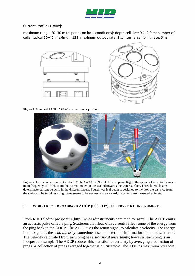
Current Profile (1 MHz):

maximum range: 20–30 m (depends on local conditions): depth cell size: 0.4–2.0 m; number of

cells: typical 20–40, maximum 128; maximum output rate: 1 s; internal sampling rate: 6 hz

Figure 1: Standard 1 MHz AWAC current-meter profiler.

Figure 2: Left: acoustic current meter 1 MHz AWAC of Nortek AS company. Right: the spread of acoustic beams of main frequency of 1MHz from the current meter on the seabed towards the water surface. Three lateral beams determinate current velocity in the different layers. Fourth, vertical beam is designed to monitor the distance from the surface. The trawl resisting frame seems to be useless and awkward, if currents are measured at inlets.

2. WORKHORSE BROADBAND ADCP (600 KHZ), TELEDYNE RD INSTRUMENTS

From RDi Teledine prospectus (http://www.rdinstruments.com/monitor.aspx): The ADCP emits an acoustic pulse called a ping. Scatterers that float with currents reflect some of the energy from the ping back to the ADCP. The ADCP uses the return signal to calculate a velocity. The energy in this signal is the echo intensity, sometimes used to determine information about the scatterers. The velocity calculated from each ping has a statistical uncertainty; however, each ping is an independent sample. The ADCP reduces this statistical uncertainty by averaging a collection of pings. A collection of pings averaged together is an ensemble. The ADCP's maximum ping rate

3

limits the time required to reduce the statistical uncertainty to acceptable levels. The ADCP measures velocities throughout the water column. The ADCP measures velocities from its transducer head to a specified range and divides this range into uniform segments called depth cells (or bins). The collection of depth cells yields a profile. (The same holds for 'stationary' AWAC profiler) The ADCP produces two profiles, one for velocity, and one for echo intensity. The ADCP calculates velocity data relative to the ADCP. The velocity data has both speed and direction information. If the ADCP is moving, and is within range of the bottom, it can obtain a velocity from returns off the bottom. This is called bottom tracking. The bottom track information can be used to calculate the absolute velocity of the water. The ADCP can get absolute direction information from a heading sensor. The following tables list the specifications for the WorkHorse ADCP. About the specifications: All these specifications assume minimal ADCP motion -pitch, roll, heave, rotation, and translation.

Key Tech specifications:

The broad bandwidth 600 MHz profiling unit reaches a range 55 m of measurements with cell heights of 0.5 m. with a standard deviation < 2 cm/s in the ansamble of 50 pings. The bottom tracking functions for bottom depths up to 100 m. According to manufacturer the bottom track velocity measurements (the velocities of a vessel) are precise to 0.6 m/s for a single ping when the speed of the vessel is 5 m/s. The accuracy of water parcels velocity is 0.25 % of the water velocity relative to the ADCP motion +/- 5 mm/s. In practice: the MBS unit of NIB is using the 600 kHz ADCP mounted at the bottom of a hull of research boat Sagita (12 m), conducting measurements with a vessel's speed 6-7 knots. However, the mountinig frame for placing the ADCP at the hull can be mounted on other (smaller) vessels as well. Four beams at the beam angle 20° from the vertical, communication RS 232 and 422, communication speed up to 115,200 baud. Sensors:

Temperature (thermistor embedded in head): range: –5 °C to +45 °C; accuracy/Resolution: –0.4

°C/0.01 °C.

Compass (flux gate with liquid tilt): maximum tilt: 15°; long term accuracy : 2.0° at 60°

magnetic dip angle accuracy/resolution: 0.5°/0.01°

4

Figure 3: RDi 600 kHz workhorse, mounted on a frame for the installation on the vessel.

Figure 4. 600 kHz ADCP RDi mounted on a bottom of the hull of Sagita.

5

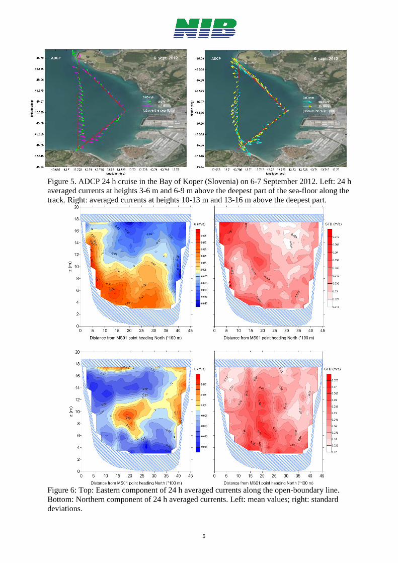
Figure 5. ADCP 24 h cruise in the Bay of Koper (Slovenia) on 6-7 September 2012. Left: 24 h averaged currents at heights 3-6 m and 6-9 m above the deepest part of the sea-floor along the track. Right: averaged currents at heights 10-13 m and 13-16 m above the deepest part.

Figure 6: Top: Eastern component of 24 h averaged currents along the open-boundary line. Bottom: Northern component of 24 h averaged currents. Left: mean values; right: standard deviations.

6

3. MICROSTRUCTURE PROFILER MSS90 SEA&SUN COMPANY

Microstructure profiler MSS90 from the German company, Sea & Sun Technology GmbH (http://www.sea-sun-tech.com/marine-tech/offshore/mss-microstructure-probe/mss-90-profiler-microstructure-probe.html) is a free falling profiler that falls with approx. constant rate 0.6-0.7 m/s. It is primarily designed to measure turbulence quantities, but the piece at MBS-NIB is adapted also for measurements of ‘usual’ oceanographic parameters adn it therefore behaves like a usual CTD with the addition of measurements of environmental parameters. MSS90 measures parameters in a vertical resolution of a few mm to a few cm. The MSS90 Profiler has 16 data channels. When the MSS90 is used as the ‘environmental CTD’ probe, then the handle with PAR is attached on top of the probe, the velocity shear is then not measured. When the MSS90 probe is to be used for turbulence profiles, then ‘ordinary’ (high accuracy and low frequency response) parameters like temperature, conductivity and pressure are still measured, however, high frequency fluctuations of temperature, conductivity and velocity shear are measured as well. Moreover, oxygen fluorescence and pH are also measured, without PAR. Mechanical parts of the profiler are constructed under the premise of a low vibration level during the sinking (or rising) movement of the instrument in water, the housing of the MSS is designed to have a resonance frequency of the first bending mode above the frequency range used for computation of turbulence parameters from the shear measurement (approx. 1-50Hz). The titanium tube housing of the standard model MSS90 is 1m long. From turbulence spectrum one estimates if for any reason there are vibrations of a probe that disturb turbulence measurements. From practice we estimate that there are no serious problems. At least three consecutive profiles at the same spot are to be performed to gain the necessary statistical significance, better five or six profiles.

Key Tech specifications:

The MSS90 Profiler at MBS-NIB is designed for vertical profiling within the upper 60 m. The MSS90 Profiler provides measurements of temperature, conductivity (salinity), oxygen, PAR, chlorophyll-a (fluorescence), pH, as well as measurements of the turbulent fluctuations in temperature and conductivity (salinity), and fluctuations of vertical shear of vortex velocities. In principal it measures turbulence in two different ways and quantities like the turbulent dissipation rate can be calculated in two ways. It includes 1,024 data sets per second; a single data set consists of 16 measured data, of which 15 are in the analog channels. The frequency width of the observation of microstructures is 150 Hz (-3dB attenuation), the instrument response time is less than 12 ms. Each channel has a resolution of 16 bits; the data transfer rate is equal to 614.4 kBaud. Standard CTD sensors (slow response but high accuracy): - Pressure (range 100 dBar, resolution 0.002% FS, accuracy: 0.1% FS, response time 150 ms) - Temperature (PT 100; range -2 … 36°C;resolution 0,0006°C, accuracy +/-0.01°C, response

time 150 ms at 1 m/s flow) - Conductivity (Principle: symmetrical cell with 7 electrodes, range 0 … 60 mS/cm, resolution

0.001 mS/cm, accuracy +/-0.02 mS/cm, response time 150 ms) - pH (combination electrode with reference, range pH 3,5 ... 10,5 resolution 0,0001 pH,

accuracy: +/-0,05 pH, response time 1 sec)

7

- Oxygen (Rinko-III optode Rockland Oceanographic Services Ltd, Response time 0.4 sec (63%), 0.9 sec (90%), range 0-200% (0 to 20 mg/L), resolution 0.01 - 0.4% (2to8 µg/L, accuracy ± 2% (at 1 atmosphere), stability ±1% (24 hours) ±5% (1 month),

- Fluorescence chl-a (Principle: fluorescence 180°, range: 0 ... 50µg/L chl-a,. resolution: 0,01 %, accuracy: 1%, response time 100 ms)

Microstructure sensors (fast response): - Microstructure temperature sensor (NTC-resistor, range: -2 ... 32°C, resolution: 0,0005°C,

accuracy: +/- 0,02°C, response time 12 ms at 1 m/s flow) - Microstructure conductivity Cm (capillary cell with two electrodes; range: 0-60 mS/cm

resolution: 1µS/cm, accuracy: 0,5 mS/cm, response time: 5 ms) - Microstructure current shear sensor SHE (piezoceramic bending element, range 0-6 Hz (10-11-

10-2 W/kg kinetic energy dissipation, resolution 10-3 Hz, resp. time: 4 ms - acceleration sensor ACC (piezoceramic bending element; range: 0-3 m/sec2; resolution: 0.005

m/sec2, accuracy: 0.02 m/sec2, response time: 4 ms)

Figure 7: Microstructure Profiler MSS90

Figure 8: The weights are located on the sensor protection cage and fixed by a clamp (photo left). The flotation rings are fixed at the upper end of the profiler housing (photo right).

8

4. VECTOR INSTRUMENT(S) FOR MEASUREMENTS OF TURBULENCE

The Vector 3D acoustic velocimeter (www.nortek-as.com) is a high-resolution acoustic velocimeter used to measure 3D water velocity in a wide variety of applications in the ocean. It samples the velocity in a small volume of water (point-wise measurements) with a volume 1 cm3. It can measure velocities with a frequency up to 64 Hz, in a continuous and in a burst mode. Key Tech specifications:

Range: 0.01 – 7.0 m/s, user selectable; accuracy 0.5 % or 1 mm/s (whichever is larger); sampling volume: 0.15 m from probe, diameter 15 mm, height 5-20 mm; uncertainty due to noise (16 Hz): 1 % of velocity range; comm. Rate: up to 115000 baud; sensors: temperature, pressure and compass/tilt; linear tilt response for inclinations up to 25°. Figure 9: Top: dimensions of the velocimeter. Bottom: left: perspective view; right: sketch of measurements with acoustic beams

9

5. SURFACE WATER SURVEY (SWS) REMOTELY CONTROLLED BOAT

Figure 10. Remote boat Čigra of MBS-NIB, designed by Franci Henigman Co. and managed by Environmental Engineering Co. (Urška Martinčič). The remotely controlled boat has been designed for measurements of surface ('skin') temperature and conductivity of water in lakes, rivers, seas, and water wells. The boat has a computer which communicates through a wireless link to a computer handled by an operator. This allows continuous monitoring of boat's position, measured quantities and battery status by the diagrams on the screen. The boat's routing is controlled digitally via radio communication with a joystick. The boat intakes water through the jet-propulsion system at a depth of only a few centimeters below the surface. Due to the continuous circulation of the water through the sensors, a continuous sampling at a rate of 10 Hz is possible. Each sample includes data of temperature, conductivity, time and DGPS position of the vessel, which allows precise temporal and spatial monitoring of route. From the measured data we can determine the salinity and density of surface waters. Surface distribution of temperature, conductivity, salinity, density and boats' route are plotted with commercial software tools (Surfer of the Golden Software Co.) Key Tech specifications:

Boat: Length: 1.31 m, weight: 9 kg, boat drive: electrical engine: 2x SPEED 700 BB TURBO; engine power: 150 W x 2; Drive: JET propulsions GPS: Javad GPS, refresh rate to 100 Hz, position accuracy up to 10 cm (in a DGPS mode) Temperature sensor: error <0.01 ° C, response time: 7 ms, measuring range: -10 to 100 ° C

10

Conductivity sensor: error <1%, response time: 2 ms, measuring range: 0.5 to 800 mS/cm The DAC interface: Data acquisition with 14-bit AD converter, absolute accuracy of data acquisition: better than 1 ‰ Computer on board: Processor: Intel ATOM N450, 1 GB of memory, 250 GB hard disk, battery duration: at least 1 h Remote Control: range: 4000 m, frequency: 2.4 GHz

Figure 11: Left: salinity distribution in the Marina Lucija (Portorož, Slovenia); Right: Temperature distribution on 27 May 2013.

11

6. SUGGESTED SCIENTIFIC REASONING AT LAKES MLJET (CRIOATIA) USING FIELD

INSTRUMENTS

There are several issues that have been raised within almost a decade of explorations of jellyfish (and other environmental issues) in Lakes Mljet. These suggestions are, of course, not obligatory and the principal investigator (Jack Costello, most likely) is free of considering anything or nothing written in this document by undersigned below. I am just ‘sick and tired’ of ‘too many secrets’ related to the new proposition and to some reservations about raising questions related to physical oceanography that should most certainly be supportive to jellyfish study. Here they are: 1. General circulation of Big lake Mljet. It is unknown – those who think that it is known, should show one single paper in a serious peer-reviewed journal, in which some modeling efforts are supported by measurements. We3 will confine ourselves to the study of the circulation of large lake, neglecting the circulation in a smaller one. It is time also for marine ecologists to know this stupid circulation, otherwise they are writing papers without knowing basics of the study environment. There are several mechanisms that need to be explored and will hardly be followed experimentally within measurements that last no longer than a week. Anyway, they should be listed as:

a) Topography control of circulation – we do expect that this matters, there are sharp topography gradients, underwater islands and so on. This is hypothesized that a Kelvin wave like circulation exists (like in the lake Kineret, Israel). This circulation could be resolved with a zig-zag 25 h cruising with a small vessel with ADCP (RDi Workhorse) mounted on the hull’s bottom. We do have experiences with this and can be done.

b) Tidal pumping of the circulation – it is important. Although all major seven tidal constituents contribute to a tidal range about 0.2 m, there are very strong (about 1 m/s) tidal currents through the tidal inlet (depth 2-3 m) that connects the Big lake with the sea. A current meter (AWAC or ADCP RDi) should be placed at the inlet’s bottom to monitor the elevation of the water in the inlet, as well as currents, to determine the phase shift between currents and elevation. The phase shift depends strongly on the volume of the lake and on the friction of the inlet. The tidal modulation of the circulation in the lake will also be detected with the above-mentioned 25 h continuous cruise campaign.

c) Wind-driven circulation: the wind filed above the lake has to be known reasonably, a few anemometers could be placed around the lake. Wind energy can matter; since the surface waves do not develop (lake is not large enough, only a few km in dimensions), the study area is simplified, majority of wind energy transforms to surface currents, which through the conservation of volume stimulate also compensating currents at depths. A possible tilt of a pycnocline at depths around 25 m during wind episode could be studied numerically and analytically, that separates the baroclinic surface motion form the (still?) layer below.

2. Barotropic generation of baroclinic internal tides Inside the lake: the inlet and the lake itself look like a perfect spot, similar to much larger seas (e.g. the Baltic Sea), which communicate with the larger water body through a narrow and shallow straight. Theories about the dissipation of barotropic energy to trigger the baroclinic internal tidaly waves with large amplitudes of vertical motion of pycnocline (thermocline) were developed in seventies and eighties of the last century (e.g. many papers of Andreas Stigebrandt from Stockholm, who has shown an interest in studying this lake from this point of view many years ago) 3. Turbulence generated along the pycnocline at depths 20-25 m: Hypothesis: Sufficiently large internal baroclinic tidal waves can cause enough vertical shear along the pycnocline during strong infow/outflow through the inlet. The gradient Richardson (Ri) number falls below 0.25 at some places inside the lake (or Ri flux number below 0.2). Then

12

a Kelvin-Helmoltz (K-H) type of instability occurs, the motion around the pycnocline is disrupted, the vertical profile of density is mixed within this layer until a ‘marginal stability’ is established (with Ri >0 0.25 – 0.3). These spots, or patches of turbulence are limited in space horizontally, as well as vertically, and their exact location inside the lake is most likely impossible to be determined. This phenomena could be hunted down by lowering the microstructure probe through the water column to see the exact location of the pycnocline, possibly also the enhanced layer of fluctuations of temperature, conductivity and velocity shear at it, or just below it. Then, at that depth the Vector instrument should be lowered at that depth to monitor continuously velocity fluctuations (with a rate of 16 Hz could be sufficient) The data come on-board of a small vessel, since the Vector is connected with a notebook via 60 m cable. In this way the K-H trubulent patch could be monitored. While the velocity fluctuations at that place are strong at that depth, the microstructure profiler will observe how large it is in height. By averaging velocity fluctuations of Vector over an interval of the order of minutes, one obtains the ‘ambient velocity’ if the horizontal motion of the instrument itself is either negligible, or somehow monitored. From the ‘mean’ horizontal velocity, and the time span of a patch, the horizontal extension of a turbulent patch could be estimated, and in combination with a height of a patch, its volume as well. If space period of transient patches could be determined, so better.

Now the ‘biology’ starts: the behavior of jellyfish in a turbulent patch vis-à-vis jellyfish community in a non-turbulent neighboring water…Most certainly very interesting stuff…

If any of the above suggestion will be accepted, we would deeply appreciate it. We would, of course, also deeply appreciate the engagement of USA experts in the above mentioned topics. Stay well, dear colleagues in Dubrovnik (Croatia) and somewhere in the USA (Woods Hole ?). Sincerely yours, Vlado Malačič Head Marine Biology Station National Institute of Biology Piran, Slovenia, 19 July 2013, malacic@mbss.org