www.rfsworld.com639

TECH

NIC

AL

INFO

RM

ATIO

N

9

Mechanical Characteristics

Cable weight

Weight per unit (meter or foot) of the complete cable.

Bending properties

A particular advantage of RF cables with corrugatedconductors is their flexibility, as expressed in the datafor minimum bending radii.

Minimum bending radius, single bending

After the cable has been bent to these minimumvalues it should not be bent back, as this could resultin damage to the cable.

Minimum bending radius, repeated bending

This bending radius allows for several operations andindicates the minimum bending radius during theinstallation procedure of the cable. It also gives anindication of the minimum reel core radius.

Bending moment

A particular advantage of RF cables with corrugatedconductors is their flexibility, as expressed in thebending moment. The cable under test is fixed in astraight support and a perpendicular force isintroduced at a certain distance (50 times the cablediameter for LCF, 25 times for SCF and UCF) awayfrom the support. The necessary force to deflect thecable by half this distance multiplied by the distancegives the bending moment.

Flat plate crush strength

Another advantage of the outer conductor corrugationis the fact that it gives the cable a very high crushresistance. If the given values are not exceeded thelocal impedance change is less than 0.5 W. Forinstance: In order to compress a 90 mm lengthsection of CELLFLEX® LCF158-50 to reduce the localimpedance by 0.5 W, it is necessary to apply a forceof more than 2790 N.

Tensile strength

The tensile strength of RF cables is determined by atypical installation situation when pulling the cablewith hoisting grips. In the case of corrugatedconductors, tensile strength is naturally less than inthe case of smooth conductors. To prevent damage tothe cable, when hoisting it into masts or pulling itthrough ducts, the maximum admissible tensile forcestated for the particular cable must not be exceeded.The values are based on a maximum cable elongationby 0.2%. Refer to the installation instructions forfurther details.

Electrical Properties

Characteristic impedance

The mean value of characteristic impedance ismeasured at around 200 MHz. The admissibledeviation from the nominal value is ± 1% to ± 4%,depending on the cable type.

Relative propagation velocity

This ratio (in percent) is the propagation velocity ofthe electromagnetic wave inside the cable in relationto propagation velocity in free space. It determines theelectrical length of the cable.

Capacitance

The capacitance of RF cables is independent offrequency and is determined by the relative dielectricconstant, the effective outer conductor diameter andthe effective inner conductor diameter.

Inductance

The inductance of RF cables is slightly frequencydependent and is determined by the effective outerand inner conductor diameter and the equivalentconducting layer due to the skin effect.

Maximum operating frequency

Up to this frequency, the properties of the cable arewithin the specifications given unless otherwise stated.

Peak power rating

Peak power rating is the input power for which thepeak RF voltage rating is reached, when the cable isoperating in its matched condition. Peak power ratingis independent of frequency.

RF peak voltage

The RF Peak voltage is limited by the air gap betweeninner and outer conductor of a coaxial line and thevoltage withstand of air. Air is also considered adielectric for foam cables since there will always be ashort section of air line at the interface between foamcable and connector. Depending on the connectorused, a smaller connector mating interface can be thelimiting factor.

Spark test

Within the production process, the cable jacket istested by applying a pulsed high voltage to the jacketagainst the outer conductor. This is to ensure theintegrity of the jacket regarding holes, inclusions andthickness.

Coaxial Transmission Lines

Definitions

9

TEC

HN

ICA

LIN

FOR

MA

TIO

N

www.rfsworld.com640

Coaxial Transmission Lines

DC-resistance inner conductor

This value is the DC-resistance of the inner conductorin ohms per length (ohms/km or ohms/1000ft).

DC-resistance outer conductor

This value is the DC-resistance of the outer conductorin ohms per length (ohms/km or ohms/1000ft).

Storage temperature

During storage the given temperature range must notbe exceeded. Otherwise the cable can be damaged.

Operation temperature

During operation the given temperature range mustnot be exceeded. Otherwise the cable can be damaged.

Installation temperature

During installation the given temperature range mustnot be exceeded. Otherwise the cable can be damaged.

Foundations

Transmission line parameters

Primary & secondary transmission lineparameters

The relation between the primary parameters:

series resistance R� in W/kminductance L� in H/kmparallel capacitance C� in F/kmparallel resistance G� in S/km

and the secondary parameters:

characteristic impedance Zc in Wpropagation constant �

phase constant � in rad/kmattenuation constant � in N/km

is given by the following transmission line equations:

� � � � j�

� � (R�� jwL�) . (G�� jwC�) (1)

Zc � (R�� jwL�) / (G�� jwC�) (2)

w � 2�f

These equations are valid for the entire frequencyrange of RF cables up to their cut-off frequency.

At radio frequencies where R� « wL� and G�« wC�, thetransmission line equations take the following form:

Zc � in W (3)

� � w . L� . C� in rad/km (4)

� � (R� / 2) / Zc � (G� / 2) . Zc

� �R � �G in nepers/km (5)

v� � 1 / L� . C� in km/s (6)

�R -conductor attenuation

�G -dielectric attenuation

v� -propagation attenuation

The deviations between equations (3) to (6) ascompared to equations (1) and (2) is below 0.1%, aslong as

De f 140 (7)

De -dielectric attenuation

f -propagation attenuation

Skin effect

At DC, current in a conductor flows with uniformdensity over the cross section of the conductor. Athigh frequencies, the current tends to flow only in theconductor surface; the effective conductor crosssection decreases and the conductor resistanceincreases.

At radio frequencies, current flows only in a very thin“skin”. Everywhere else the conductors are free fromelectromagnetic fields. Even very thin walled metalenvelopes will, therefore, entirely screen the electro-magnetic field within coaxial RF cables atradio frequencies.

L�

C�

www.rfsworld.com641

TECH

NIC

AL

INFO

RM

ATIO

N

9

Coaxial Transmission Lines

10-6 . er

18 . In (Dc /dc)

Di + ddi - d

The depth of penetration illustrates the skin effect. Itis defined as the thickness of a thin surface layer(assumed to have an even distribution of currentflow), having the same resistance as an actualconductor, which is undergoing to the skin effect.

For non-magnetic materials the equivalent conductinglayer is

d � 15, 9 / s . f in mm (8)

s - conductivity in m/W mm2

f - frequency in kHz

Other than resistance, the skin effect also influencesinductance and thereby characteristic impedance andpropagation velocity.

Electrical characteristics

Capacitance

The capacitance of RF cables is independent offrequency:

C� � in F/km (9)

er - relative dielectric constant

Dc - effective outer conductor diameter (capacitive)

dc - effective inner conductor diameter(capacitive)

Inductance

The inductance of a RF cable is:

L� � 2 . 10-4 . In in H/km (10)

Di - effective inner conductor diameter (inductive)

di - effective inner conductor diameter (inductive)

d - equivalent conducting layer

At very high frequencies, inductance approaches:in H/km

L� � 2 . 10-4 . In(Di / di) in H/km (11)

Characteristic impedance

The characteristic impedance of an RF cable isdetermined by its inductance and capacity accordingto equation 3. Because of the influence of the skineffect upon inductance, it also is frequency-dependent.

Characteristic impedance of RF cables is, therefore,understood as the value it approaches for very highfrequencies. If we say Dc = Di = De , dc = di = de

and d « di then

Zc � . In(De / de) in W (12)

De - electrically effective outer conductor

diameter

de - electrically effective inner conductor

diameter

er - relative dielectric constant

As frequency falls, the characteristic impedance rises.The relative deviation from the value at very highfrequency is approx.

�

De - electrically effective outer conductor in mm

f - frequency in kHz

Certain electrical properties of an RF cable can beoptimized by proper choice of characteristicimpedance. For coaxial cables with cylindricalconductors (of the same material) the followingoptimizations are possible:

AIR DIELECTRIC SOLID PECABLES DIELECTRIC CABLES

minimum attenuation 77 ohms 51 ohmsmax. operating voltage 60 ohms 40 ohmsmax. peak power rating 30 ohms 20 ohmsmax. mean power rating =50 ohms*

*approx. valid for HELIFLEX® transmission lines of larger diameter

D Z

Zc

4

De. f

60

er

9

TEC

HN

ICA

LIN

FOR

MA

TIO

N

www.rfsworld.com642

Coaxial Transmission Lines

Today, RF coaxial cables are produced mainly withcharacteristic impedance of 50 ohms and to someextend in 75 ohms.

As the material properties and dimensions of RFcables are not constant along their length, the charac-teristic impedance will vary with length and deviatefrom the mean value of characteristic impedance ofthe particular cable; similarly the mean value willdeviate from the nominal value (50 or 75 ohms).

The mean value of characteristic impedance of a cableis defined as follows:

Zm � in ohms (14)

Ie - electrical length in m

co - propagation velocity in

free space in m/sec

C - capacitance in F

The mean value of characteristic impedance ismeasured at around 200 MHz. The admissibledeviation from the nominal value is ¾ 1% to ¾4%, depending on the product group.

Uniformity of characteristic impedance

As mentioned, the material properties of RF cables arenot uniform along their length and result in smalldeviations of the characteristic impedance. Theimpedance step D Z at position x of the cable resultsin reflection factor at the position as follows:

rx � (15)

The magnitude and distribution of the variousreflections determine their effect upon transmissionproperties. Two ways are commonly used to judge theeffect of impedance variation.

Time domain reflectometry (TDR)

A defined voltage step is fed into the cable andpartially reflected at each impedance variation. Thedisplay of the reflected energy versus time gives aview upon the local distribution of the innerreflections. The pulse reflection factor at a certainposition is the ratio between the voltage of thereflected and the incident pulse. Instead of reflectionfactor, one can also use the term pulse return loss:

Ap = 20 . log in dB (16)

rp - pulse reflection in %factor

The magnitude and nature of the pulse reflectionfactor depend very much upon the form of incident pulse.

Return loss/reflection factor (steady state condition)

The reflection factor sums up the effects of all theimpedance variations within the cable and its ends, ata certain frequency. It is the ratio between thevectorial) addition of all reflections and the incidentsignal, measured at the near end of the cable.

As well as reflection factor, the term return loss is also used.

Az = 20 . log in dB (17)

r - reflection factor in %

The reflection factor versus frequency may be plottedcontinuously. The reference impedance of testequipment and the load at cable end are equal to thenominal value of cable impedance.

It is also customary to use the term voltage standingwave ratio (VSWR), based upon the standing wave,which the cable under test would produce in ahomogeneous transmission line connected to its nearend and having its nominal characteristic impedance.

s = (18)

r = . 100 in % (19)

s - standing wave ratio

Relative propagation velocity and delay

The relative propagation velocity is defined as follows.

nr = . 100 = . 100 in % (20)

u� - propagation velocity in cable

Ie

co. C

D Z

2Zc

100

rp

100

r

1 � r / 100

1 � r / 100

s � 1

s � 1

u�

co

l

le

www.rfsworld.com643

TECH

NIC

AL

INFO

RM

ATIO

N

9

Coaxial Transmission Lines

co- propagation velocity in free space (300•103 km/s)

l - geometrical in mlength

le - electrical length in m

Delay is defined as follows:

t� = = in ns/m (21)

nr - relative propagation velocity in %

Due to the skin effect, propagation velocity isfrequency dependent. Velocity decreases with fallingfrequency, delay increases. The relative deviation canbe calculated according to equation 13.

As in the case of characteristic impedance, relativepropagation velocity of RF cables is understood as thevalue it approaches for very high frequencies. If Dc =Di and dc = di it is dependent solely upon thedielectric constant and is defined as follows:

nr = in % (22)

Propagation velocity is measured at frequenciesaround 200 MHz as standard. Propagation velocity isalso subject to variations. These variations have nodirect influence upon transmission characteristics;they do, however, come to light, if cables have to beadjusted to equal electrical length, because afteradjustment the cables of equal electrical length mayshow differences in geometrical length. If cables are tobe used in applications where consistency of electricallength is important, we recommend that this is statedat the time of order placement, in order to allow us toselect the cables from one manufacturing batch,whenever possible.

Electrical length and adjustment of length

The electrical length is defined as follows:

le = in m (23)

l - geometrical in mlength

nr - relative propagation velocity in %

Between electrical length and phase angle thefollowing relation applies:

� = 2 . . f in rad (24)

le - electrical length in m

f - frequency in MHz

In many cases, cables with equal or defined differ-ential electrical length are required. Typical examplesare feeder cables for TV transmitters and cabling ofantenna groups or antenna arrays. Such lengthadjustments can be made with precision. A typicalvalue for the achievable accuracy is a phase angletolerance of ± 5° in the 470 to 860 MHz frequencyband. In order to eliminate length variations throughhandling after adjustment, we recommend to havelong lengths of cables length adjusted after instal-lation; short cable lengths may, however, be suppliedfactory-adjusted.

The electrical length of RF cables is dependent upontemperature, and in case of air dielectric cables alsoupon the pressure and humidity of contained air. Theinfluences are quite small, but must, however, betaken into account in case where the cables are verylong as compared to the operating wavelength.

It is advisable to install length-adjusted cables so thatthey are all subject to the same ambient conditionssuch as temperature, solar radiation etc. Length-adjusted HELIFLEX® cables should be operated undera slight overpressure (the same for all cables) ofapprox. 0.2 bar of dry air or nitrogen.

For less critical applications, phase-stabilized cablescan be supplied. These are cables that are aged inorder to reduce hysteresis effects.

The variation of electrical length with temperature isalso influenced by the kind of cable attachment to thesupport structure. Cables that can expand freely withtemperature have different values than cables whichare rigidly clamped down.

In the following diagrams typical figures of theelectrical length change are shown for severalcable types.

336.6nr

108

nr. co

100

er

100 . lnr

1e

300

9

TEC

HN

ICA

LIN

FOR

MA

TIO

N

www.rfsworld.com644

Coaxial Transmission Lines

The phase change for a given cable length andtemperature range can be calculated with equation(25).

D� = 120 . 10-6 . . Dppm . f

in Deg (25)

l - cable length in m

nr - relative propagation velocity in %

Dppm - electrical length in m

change

f - frequency in MHz

Example:A 10 m run of LCF12-50 is used in the temperaturerange from -10°C to 40°C (14°F to 104°F) at 1 GHz.

In the above diagram the Dppm of approximately 280can be read. The maximum phase change is

D� = 120 . 10-6 . . 280 . 1000 = 3.8°

Attenuation

The attenuation of RF cables is defined as follows:

� � 10 . log(P1 / P2) in dB/100 m (26)

P1 - input power into a 100 m long cable terminatedwith the nominal value of its characteristic impedance

P2 - power at the far end of this cable

The construction of a cable influences the attenuation(in the case of copper conductors and at 20°C [68°F])in accordance with the following equation:

�20 � ( � ) . f � 9,1 . er. tgd . f

� �R � �G in dB/100 m (27)

Zc characteristic impedance in ohm

f frequency in MHz

De electrically equivalent outer conductordiameter in mm

de electrically equivalent inner conductordiameter in mm

er relative permittivity of dielectric

tgd loss factor of dielectric

ki shape factor of inner conductor

ka shape factor of outer conductor

LCF-Cables

-600

-500

-400

-300

-200

-100

0

100

200

-30 -25 -20 -15 -10 -5 0 5 10 15 20 25 30 35 40 45 50 55 60 65

Temperature [˚C]

Elec

tric

al L

eng

th C

han

ge

[p

pm

]

LCF38-50J-TC

LCF12-50J-TC

LCF58-50J-TC

LCF-Cables

-900

-800

-700

-600

-500

-400

-300

-200

-100

0

100

-30 -25 -20 -15 -10 -5 0 5 10 15 20 25 30 35 40 45 50 55 60 65

Temperature [˚C]

Elec

tric

al L

eng

th C

han

ge

[p

pm

]

LCF78-50J-TC

LCFS114-50J-TC

LCF158-50J-TC

SCF-Cables

-900

-800

-700

-600

-500

-400

-300

-200

-100

0

100

200

-30 -25 -20 -15 -10 -5 0 5 10 15 20 25 30 35 40 45 50 55 60 65

Temperature [˚C]

Elec

tric

al L

eng

th C

han

ge

[p

pm

]

SCF14-50J-TC

SCF38-50J-TC

SCF12-50J-TC

HCA-Cables

-700

-600

-500

-400

-300

-200

-100

0

100

200

300

400

500

-30 -25 -20 -15 -10 -5 0 5 10 15 20 25 30 35 40 45 50 55 60 65

Temperature [˚C]

Elec

tric

al L

eng

th C

han

ge

[p

pm

]

HCA38-50J-TC

HCA58-50J-TC

HCA78-50J-TC

1

vr

36, 1

Zc

ki

de

ka

De

10

88

www.rfsworld.com645

TECH

NIC

AL

INFO

RM

ATIO

N

9

Coaxial Transmission Lines

The attenuation values are stated for 20 °C (68°F). Thestated figures are typical. With rising ambienttemperature the attenuation also rises, by 0.2% K. Theattenuation also rises if the cable is heated up by thetransmitted power. The maximum rise is as follows:

HELIFLEX® cable with PE dielectric �t/�20 � 1.14

HELIFLEX® cable with PTFE dielectric �t/�20 � 1.20

CELLFLEX® cable �t/�20 � 1.12

�t - attenuation of the cable at full mean powerrating

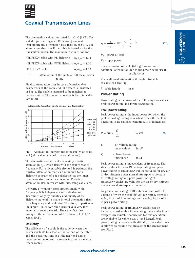
Finally, attenuation rises in case of considerablemismatches at the cable end. The effect is illustratedin Fig. 1. The cable is assumed to be matched at the transmitter. The curve parameter is the total cableloss in dB.

Fig. 1 Attenuation increase due to mismatch at cableend (with cable matched at transmitter end)

The attenuation of RF cables is mainly resistiveattenuation �r , which rises with the square root offrequency. For a given cable size and impedance, theresistive attenuation reaches a minimum for adielectric constant of 1 (air dielectric) as the innerconductor size reaches a maximum. Resistiveattenuation also decreases with increasing cable size.

Dielectric attenuation rises proportionally withfrequency. It is independent of cable size anddetermined only by quantity and quality of thedielectric material. Its share in total attenuation riseswith frequency and cable size. Therefore, in particularthe larger HELIFLEX® cable sizes have a very lowmaterial content dielectric. The same fact alsoprompted the introduction of loss foam CELLFLEX®cables (LCF).

Efficiency

The efficiency of a cable is the ratio between thepower available to a load at the far end of the cableand the power put into it at the near end and istherefore an important parameter to compare severalfeeder cables.

� � � 10- (28)

P2 - power at load

P1 - input power

�t - attenuation of cable (taking into accountadditional attenuation due to the power being used)

in dB/100 m

Ar - additional attenuation through mismatch at cable end (see Fig.1)

l - cable length in m

Power Rating

Power rating is the lower of the following two values:peak power rating and mean power rating.

Peak power rating

Peak power rating is the input power for which thepeak RF voltage rating is reached, when the cable isoperating in its matched condition. It is defined as:

P � 500 . in kW (29)

U - RF voltage rating(peak value) in kV

Zc - characteristicimpedance in W

Peak power rating is independent of frequency. Thestated values for peak RF voltage rating and peakpower rating of HELIFLEX® cables are valid for dry airor dry nitrogen under normal atmospheric pressure.RF voltage rating and peak power rating ofHELIFLEX® cables are valid for dry air or dry nitrogenunder normal atmospheric pressure.

As production testing of RF cables is done with DCvoltage of twice the peak RF voltage rating, there is asafety factor of 2 in voltage and a safety factor of 4in peak power rating.

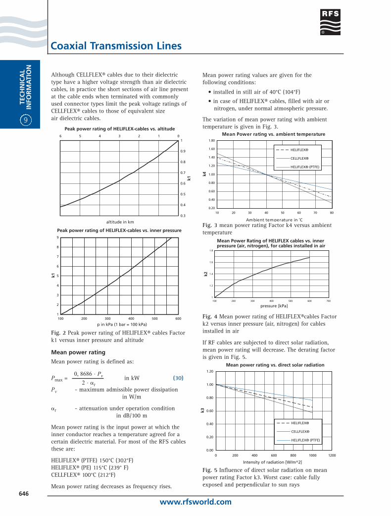
Peak power rating of HELIFLEX® cables can beincreased considerably by operating them under inneroverpressure (suitable connectors for this operationare available for cable, sizes 3¨ and larger). Peakpower rating decreases with altitude, if the cable inneris allowed to assume the pressure of the environment,see. Fig. 2.

Additional attenuation due to mismatch of termination

0.0

0.1

0.2

0.3

0.4

0.5

1 1.2 1.4 1.6 1.8 2

mismatch at cable end VSWR

atte

nu

atio

n in

crea

se in

dB

0,5 dB

1 dB

2 dB

3 dB

6 dB

absolute cable loss

P2

P1 10

�t. �Ar

( )

l

100

U

Zc

9

TEC

HN

ICA

LIN

FOR

MA

TIO

N

www.rfsworld.com646

Although CELLFLEX® cables due to their dielectric type have a higher voltage strength than air dielectriccables, in practice the short sections of air line presentat the cable ends when terminated with commonlyused connector types limit the peak voltage ratings ofCELLFLEX® cables to those of equivalent size air dielectric cables.

Fig. 2 Peak power rating of HELIFLEX® cables Factork1 versus inner pressure and altitude

Mean power rating

Mean power rating is defined as:

Pmax = in kW (30)

Pv - maximum admissible power dissipationin W/m

�t - attenuation under operation condition in dB/100 m

Mean power rating is the input power at which theinner conductor reaches a temperature agreed for acertain dielectric material. For most of the RFS cablesthese are:

HELIFLEX® (PTFE) 150°C (302°F)HELIFLEX® (PE) 115°C (239° F)CELLFLEX® 100°C (212°F)

Mean power rating decreases as frequency rises.

Mean power rating values are given for the following conditions:

• installed in still air of 40°C (104°F)

• in case of HELIFLEX® cables, filled with air ornitrogen, under normal atmospheric pressure.

The variation of mean power rating with ambienttemperature is given in Fig. 3.

Fig. 3 mean power rating Factor k4 versus ambienttemperature

Fig. 4 Mean power rating of HELIFLEX®cables Factork2 versus inner pressure (air, nitrogen) for cablesinstalled in air

If RF cables are subjected to direct solar radiation,mean power rating will decrease. The derating factoris given in Fig. 5.

Fig. 5 Influence of direct solar radiation on meanpower rating Factor k3. Worst case: cable fullyexposed and perpendicular to sun rays

Mean Power rating vs. ambient temperature

0.20

0.40

0.60

0.80

1.00

1.20

1.40

1.60

1.80

10 20 30 40 50 60 70 80

Ambient temperature in ˚C

k4

HELIFLEX®

CELLFLEX®

HELIFLEX® (PTFE)

Mean Power Rating of HELIFLEX cables vs. inner pressure (air, nitrogen), for cables installed in air

1

1.2

1.4

1.6

1.8

100 200 300 400 500 600 700

pressure [kPa]

k2

Mean power rating vs. direct solar radiation

0.00

0.20

0.40

0.60

0.80

1.00

1.20

0 200 400 600 800 1000 1200

Intensity of radiation [W/m^2]

k3

HELIFLEX®

CELLFLEX®

HELIFLEX® (PTFE)

1

2

3

4

5

6

7

8

9

100 200 300 400 500 600

p in kPa (1 bar = 100 kPa)

k1

Peak power rating of HELIFLEX-cables vs. inner pressure

0.3

0.4

0.5

0.6

0.7

0.8

0.9

10123456

altitude in km

k1

Peak power rating of HELIFLEX-cables vs. altitude

0, 8686 . Pv

2 . �t

Coaxial Transmission Lines

www.rfsworld.com647

TECH

NIC

AL

INFO

RM

ATIO

N

9

Power considerations summary

If the cable end is not terminated in its characteristicimpedance, standing waves along the cable will resultin higher power being dissipated at current andvoltage maximums. Input power must, therefore, bereduced accordingly. In summary, therefore, thefollowing conditions must be fulfilled when selectinga cable size for a certain power configuration.

Pmax (31)

Pmax P (32)

P, P - peak power and mean power of transmitter

Pmax, Pmax- peak power rating and mean powerrating of cable

s - VSWR

k1 - peak power rating factor for inner pressure(Fig. 2)

k2 - mean power rating factor for inner pressure (Fig. 4)

k3 - mean power rating factor for direct solarradiation (Fig. 5)

k4 - mean power rating factor for ambienttemperature (Fig. 3)

For cables operated above half their cut-off frequencyin a non-matched condition, heat compensationbetween the extreme values of temperature along thecable can be expected. In this case, the VSWR inequation 32 may be replaced by the term:

(s2 + 1) / 2 s

Coaxial Transmission Lines

For mean power calculation of cables to be buried inthe ground, the heat resistance of the cable jacket toair combination is replaced by the heat resistance ofthe soil, and the ambient temperature is replaced bythe average soil temperature at the proposed cable laying depth.

As the heat resistivity of the soil is very dependentupon local conditions such as humidity and type ofsoil, and since the soil in the vicinity of RF cableswhich dissipate large heat power tends to dry out, it isnecessary to have the correspondent information fromthe list given below.

Generally, it can be said for normal kinds of soil inmoderate climates, that mean power rating of smallercable sizes (if buried) increases whereas in the case oflarger cable sizes it decreases.

If a buried, large cable is operating under inneroverpressure, mean power rating doesn’t increase asmuch as if this cable would be installed aboveground.

When planning an RF cable system the followingData should be known:

Installation location details:

• height above sea level

• ambient temperature and intensity of solar radiation

• ground temperature, soil type and ground water level

Installation details:

• cable to be laid in masts, above-ground, in-ground or in ducts

• pressurization permissible

• heat dissipated by parallel cables

• connector types

Operating conditions:

• number and length of cables

• frequencies and permissible attenuation

• transmitter peak and average output power(P and P )

• or the information to calculate these data, asgiven in Fig.6 antenna VSWR (s)

sk2k3k4

P . sk1

9

TEC

HN

ICA

LIN

FOR

MA

TIO

N

www.rfsworld.com648

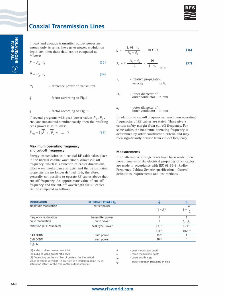
If peak and average transmitter output power areknown only in terms like carrier power, modulationdepth etc., then these data can be computed asfollows:

P � PR. q (33)

P � PR. q (34)

PR - reference power of transmitter

q - factor according to Fig.6

q - factor according to Fig. 6

If several programs with peak power values P1 , P2 ,etc., are transmitted simultaneously, then the resultingpeak power is as follows:

Pres = ( P1 + P2 + ..........)2 (35)

Maximum operating frequency and cut-off frequency

Energy transmission in a coaxial RF cable takes placein the normal coaxial wave mode. Above cut-offfrequency, which is a function of cables dimensions,other wave modes can also exist and the transmissionproperties are no longer defined. It is, therefore,generally not possible to operate RF cables above theircut-off frequency. An approximate value of cut-offfrequency and the cut-off wavelength for RF cablescan be computed as follows:

Coaxial Transmission Lines

fc = in GHz (36)

c = p . (37)in m

vr - relative propagationvelocity in %

Di - inner diameter of outer conductor in mm

da - outer diameter of inner conductor in mm

In addition to cut-off frequencies, maximum operatingfrequencies of RF cables are stated. These give acertain safety margin from cut-off frequency. Forsome cables the maximum operating frequency isdetermined by other construction criteria and maythen significantly deviate from cut-off frequency.

Measurements

If no alternative arrangements have been made, thenmeasurements of the electrical properties of RF cablesare made in accordance with IEC 61196-1: Radio-Frequency-Cables; Generic specification - Generaldefinitions, requirements and test methods.

MODULATION REFERENCE POWER PR q qamplitude modulation carrier power

(1 + m)2 1 +

frequency modulation transmitter power 1 1pulse modulation pulse power 1 tp . fptelevision (CCIR Standard) peak sync. Power 1.73 [1] 0.71 [1]

1.50 [2] 0.66 [2]

DAB OFDM sum power 10 [3] 1DVB OFDM sum power 10 [3] 1

m2

2

1, 91 . vr

Di + da

Di + da

2

10

1 . vr

Fig. 6

[1] audio to video power ratio 1:10[2] audio to video power ratio 1:20[3] Depending on the number of carriers, the theoreticalvalue of can be very high. In practice, it is limited to about 10 bysaturation effects of the transmitter output amplifier.

m - peak modulation depthm - mean modulation depthtp - pulse length in ms

fp - pulse repetition frequency in MHz

www.rfsworld.com649

TECH

NIC

AL

INFO

RM

ATIO

N

9

Base Station Antenna Systems

Propagation

Need: The aim of telecommunications is to transmit,from one point to another, a signal carrier of aninformation.

Medium: Propagation of electromagnetic energybetween a transmitter and a receiver.

Modes: Propagation in free space (without physicalmedium).

Antenna

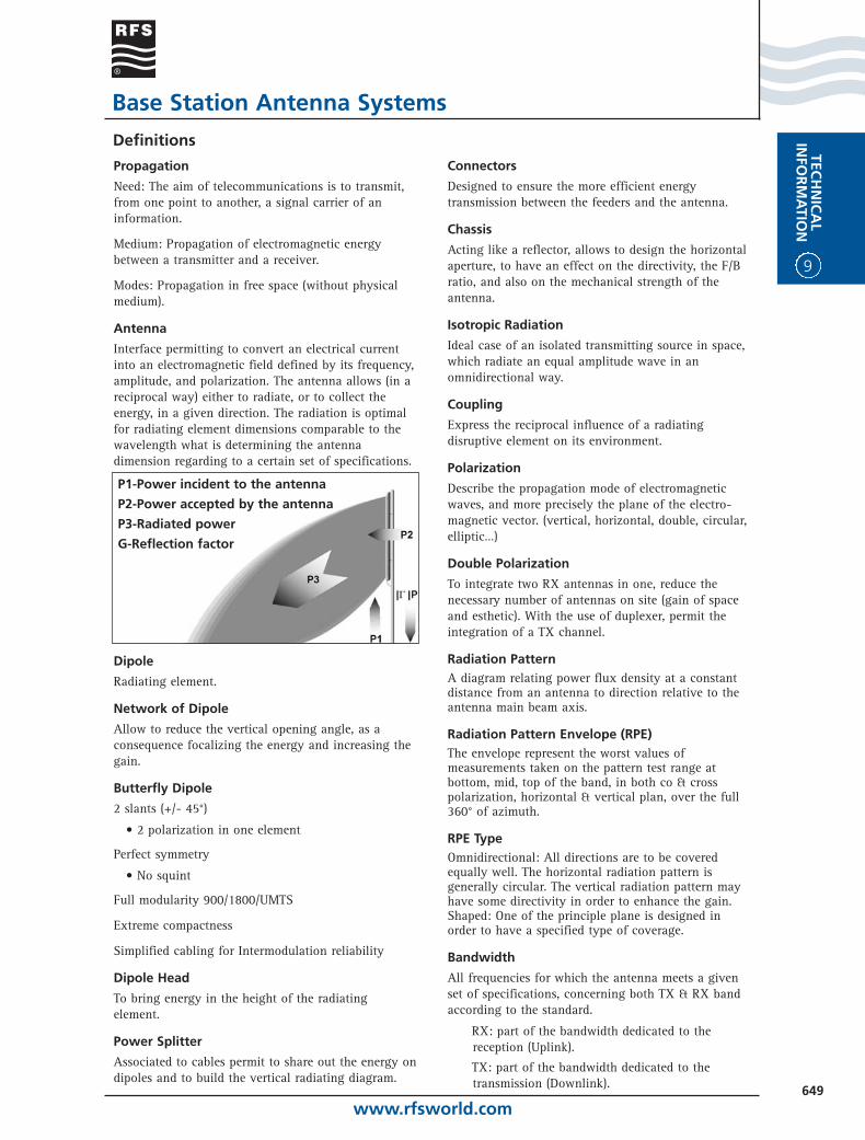
Interface permitting to convert an electrical currentinto an electromagnetic field defined by its frequency,amplitude, and polarization. The antenna allows (in areciprocal way) either to radiate, or to collect theenergy, in a given direction. The radiation is optimalfor radiating element dimensions comparable to thewavelength what is determining the antennadimension regarding to a certain set of specifications.

Dipole

Radiating element.

Network of Dipole

Allow to reduce the vertical opening angle, as aconsequence focalizing the energy and increasing thegain.

Butterfly Dipole

2 slants (+/- 45°)

• 2 polarization in one element

Perfect symmetry

• No squint

Full modularity 900/1800/UMTS

Extreme compactness

Simplified cabling for Intermodulation reliability

Dipole Head

To bring energy in the height of the radiatingelement.

Power Splitter

Associated to cables permit to share out the energy ondipoles and to build the vertical radiating diagram.

Connectors

Designed to ensure the more efficient energytransmission between the feeders and the antenna.

Chassis

Acting like a reflector, allows to design the horizontalaperture, to have an effect on the directivity, the F/Bratio, and also on the mechanical strength of theantenna.

Isotropic Radiation

Ideal case of an isolated transmitting source in space,which radiate an equal amplitude wave in an omnidirectional way.

Coupling

Express the reciprocal influence of a radiatingdisruptive element on its environment.

Polarization

Describe the propagation mode of electromagneticwaves, and more precisely the plane of the electro-magnetic vector. (vertical, horizontal, double, circular,elliptic…)

Double Polarization

To integrate two RX antennas in one, reduce thenecessary number of antennas on site (gain of spaceand esthetic). With the use of duplexer, permit theintegration of a TX channel.

Radiation PatternA diagram relating power flux density at a constantdistance from an antenna to direction relative to theantenna main beam axis.

Radiation Pattern Envelope (RPE)The envelope represent the worst values ofmeasurements taken on the pattern test range atbottom, mid, top of the band, in both co & crosspolarization, horizontal & vertical plan, over the full360° of azimuth.

RPE TypeOmnidirectional: All directions are to be coveredequally well. The horizontal radiation pattern isgenerally circular. The vertical radiation pattern mayhave some directivity in order to enhance the gain.Shaped: One of the principle plane is designed inorder to have a specified type of coverage.

Bandwidth

All frequencies for which the antenna meets a givenset of specifications, concerning both TX & RX bandaccording to the standard.

RX: part of the bandwidth dedicated to thereception (Uplink).

TX: part of the bandwidth dedicated to thetransmission (Downlink).

P1-Power incident to the antenna

P2-Power accepted by the antenna

P3-Radiated power

G-Reflection factor

Definitions

9

TEC

HN

ICA

LIN

FOR

MA

TIO

N

www.rfsworld.com650

Base Station Antenna Systems

Uplink

Transmitting direction from the mobile to the BTS.

Downlink

Transmitting direction from the BTS to the mobile.

Fading

The existence of various type of obstacles, generatereflections and diffraction of the transmitted wave.The uplink suffer generally of wide amplitudevariations: Shadowing / path loss / multi-pathpropagation. The received signal is summation ofseveral rays, sometimes leading to cancellation(regarding to the phase), which causes a drop call.

Multipath propagation

The mobile and environment moving induce adiscrepancy on received signal frequencies.

Analog signal: intermodulation noise.

Digital noise: increase of the bit error rate.

Diversity Definitions

Solution designed in view of improving the drop call

Space diversity

Horizontal separation of 2 antennas for receive path.

Drawbacks:Visual impact, heavy and expensive platform, largespace requirement.

Benefits:• Optimum gain for wide area.

• Normal spacing = l

• 6 m (20 ft) spacing in 800-900 MHz

• 3 m (10 ft) spacing in 1800-1900 MHz

Polarization diversity

Reception on perpendicular radiating elements (crosspol antenna): physical spacing no longer needed. Maybe associated to the cross polarization discrimination.

Horizontal/Vertical slants —

Drawbacks:Problem to achieve good isolation between eachports. Unbalanced RX signal reduce polarizationdiversity. No possible Horizontal transmit.

Benefits:• Optimal Vertical transmit

• +/- 45° slants —

Drawbacks:

Worse propagation in free space.

Benefits:• Full RX TX equivalent propagation.• Equivalent mean signal.• H /V polarized coverage equivalent

Signal’s Selection —

Selection diversity (Best SNR)Maximum ratio (Amplitude or phase, or both)

Downtilt Definitions

Control of the signal such as the focus is below thehorizon. Downtilt can be potentially achievedmechanically, electrically or with a combination of thetwo. Associated to the RET system, Downtilt could bedone remotely. Downtilt improves coverage close tothe site, reduce the cell site radius & interferences.

Mechanical downtilt / uptilt

Achieved by the mounting hardware.

Drawbacks:Weaker mechanically, non-regular coveragereduction, notch effect in main direction,interference reduction in main direction only, not good for visual impact.

Benefits:• Adjustment on site.

Electrical downtilt

Fixed electrical tilt —

Drawbacks:Total freedom on site only with tuneable tilt.

Benefits:• All lobes equally tilted• Equal reduction of all interferences• Regular reduction of coverage• Best solution for visual impact• Good mechanical withstanding

Variable electrical tilt —

Benefits:• Easy cell size tuning according to capacity

evolution• Full network planning freedom.• Keep low interferences• Prevent change of antenna• IMP free antenna providing no additional

galvanic contact thanks to the dielectric built inVET system.

Remote electrical tilt —

Benefits:• RET will provide interference mastering.• Reduction of cells overlapping.• Coverage versus Capacity easy adaptation.• Fine Cell’s tuning without sending crew on the

site.• Control of non accessible sites.• Reduction of Network Optimization’s cost.• No limitation on frequency of tuning.• Compatible with future dynamic capacity

allocation

Definitions

www.rfsworld.com651

TECH

NIC

AL

INFO

RM

ATIO

N

9

Base Station Antenna Systems

Side by Side Configuration

Dual band application

2 single band antennas placed closed together in asingle radome.

Benefits:• Reaches the better performance on each band.

• Efficient interband isolation performance.

• Manages the external aspect.

Air combining application

Allows 3 dB saving in power budget.2 identical antennas in view of having a thinnerhorizontal beamwidth. (Generally 2 times thinner thanthe HPBW obtained with a single band one).

Concentric cell application

2 antennas with the same gain, but different tilts (fordifferent coverage policy).

Side sharing application

Different range of GSM1800/1800, PCC1900/1900,GSM1800/UMTS, UMTS/UMTS solution in order tomanage site reuse between various operators, withoutsite extra-negotiation.

Tower Mounted Amplifier (TMA)

Benefits:• Fewer cell sites by increasing cell size.

• Improved coverage.

• Reduction of drop call.

• Improve uplink power budget — leads to a longerhandset battery life size

• Compatible to all BTS providers.

• High reliability.

Definitions

9

TEC

HN

ICA

LIN

FOR

MA

TIO

N

www.rfsworld.com652

Base Station Antenna Systems

Single band

Antenna developed for the coverage of oneparticular standard.Optimized for the narrow band requirement.

Broad band

Antenna developed for the coverage of at least twodifferent standards. Approached as a compromise dueto the larger band aspect.

Multi band

Several dipole networks cohabiting in the samechassis: Dual band / Triple band antennas.

Network Planning

Cellular systems

The approximation of each cell represents a hexagon.

Low Power of transmitters induce:• A limited range.

• Space split in elementary cells.

Reducing interferences induce:• Space between frequencies.

• (limited spectrum/frequency reuse/largenumber of cells).

Deployment

Depends on:• The number of simultaneous communications to

sell.

• The relief of the covered area.

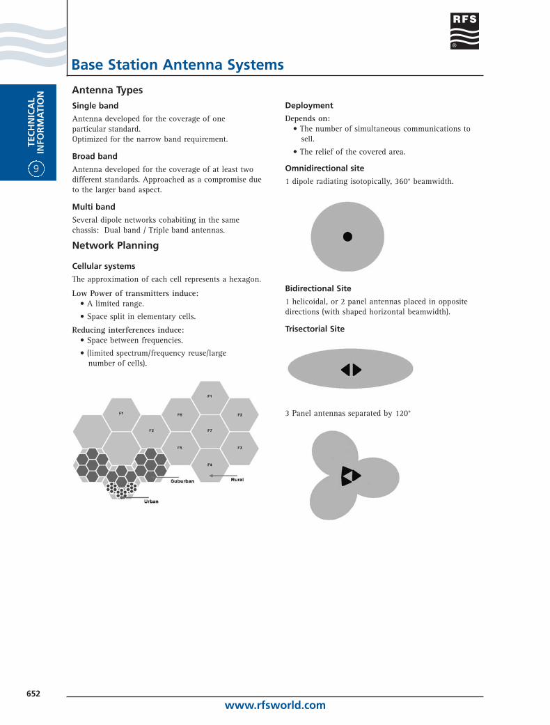
Omnidirectional site

1 dipole radiating isotopically, 360° beamwidth.

Bidirectional Site

1 helicoidal, or 2 panel antennas placed in oppositedirections (with shaped horizontal beamwidth).

Trisectorial Site

3 Panel antennas separated by 120°

Antenna Types

www.rfsworld.com653

TECH

NIC

AL

INFO

RM

ATIO

N

9

Base Station Antenna Systems

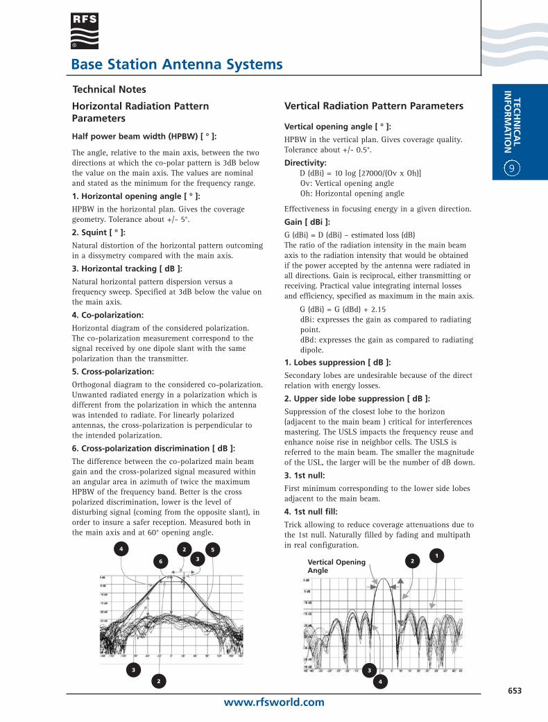
Horizontal Radiation PatternParameters

Half power beam width (HPBW) [ ° ]:

The angle, relative to the main axis, between the twodirections at which the co-polar pattern is 3dB belowthe value on the main axis. The values are nominaland stated as the minimum for the frequency range.

1. Horizontal opening angle [ ° ]:

HPBW in the horizontal plan. Gives the coveragegeometry. Tolerance about +/- 5°.

2. Squint [ ° ]:

Natural distortion of the horizontal pattern outcomingin a dissymetry compared with the main axis.

3. Horizontal tracking [ dB ]:

Natural horizontal pattern dispersion versus afrequency sweep. Specified at 3dB below the value onthe main axis.

4. Co-polarization:

Horizontal diagram of the considered polarization.The co-polarization measurement correspond to thesignal received by one dipole slant with the samepolarization than the transmitter.

5. Cross-polarization:

Orthogonal diagram to the considered co-polarization.Unwanted radiated energy in a polarization which isdifferent from the polarization in which the antennawas intended to radiate. For linearly polarizedantennas, the cross-polarization is perpendicular tothe intended polarization.

6. Cross-polarization discrimination [ dB ]:

The difference between the co-polarized main beamgain and the cross-polarized signal measured withinan angular area in azimuth of twice the maximumHPBW of the frequency band. Better is the crosspolarized discrimination, lower is the level ofdisturbing signal (coming from the opposite slant), inorder to insure a safer reception. Measured both inthe main axis and at 60° opening angle.

Vertical Radiation Pattern Parameters

Vertical opening angle [ ° ]:

HPBW in the vertical plan. Gives coverage quality.Tolerance about +/- 0.5°.

Directivity:D (dBi) = 10 log [27000/(Ov x Oh)]Ov: Vertical opening angleOh: Horizontal opening angle

Effectiveness in focusing energy in a given direction.

Gain [ dBi ]:

G (dBi) = D (dBi) – estimated loss (dB)The ratio of the radiation intensity in the main beamaxis to the radiation intensity that would be obtained if the power accepted by the antenna were radiated inall directions. Gain is reciprocal, either transmitting orreceiving. Practical value integrating internal losses and efficiency, specified as maximum in the main axis.

G (dBi) = G (dBd) + 2.15dBi: expresses the gain as compared to radiatingpoint.dBd: expresses the gain as compared to radiatingdipole.

1. Lobes suppression [ dB ]:

Secondary lobes are undesirable because of the directrelation with energy losses.

2. Upper side lobe suppression [ dB ]:

Suppression of the closest lobe to the horizon(adjacent to the main beam ) critical for interferencesmastering. The USLS impacts the frequency reuse andenhance noise rise in neighbor cells. The USLS isreferred to the main beam. The smaller the magnitudeof the USL, the larger will be the number of dB down.

3. 1st null:

First minimum corresponding to the lower side lobesadjacent to the main beam.

4. 1st null fill:

Trick allowing to reduce coverage attenuations due tothe 1st null. Naturally filled by fading and multipathin real configuration.4

6

3

2

2

3

5

Technical Notes

21

3

4

Vertical OpeningAngle

9

TEC

HN

ICA

LIN

FOR

MA

TIO

N

www.rfsworld.com654

Base Station Antenna Systems

Other Parameters

Voltage standing wave ratio [ VSWR ]

Capacity of the antenna in radiating the energywithout reflecting a part towards the BTS. Faculty ofantenna impedance matching to system impedance.Value guaranteed across the frequency band ofoperation.

Impedance [ WW ]

Fundamental electrical parameter allowing thecomplete adaptation between the antenna and thefeeding system. Fixed as a standard at 50W.

Front to back ratio [ dB ]• Denotes the highest level of radiation relative to

the main beam in an angular area of 180o +/-40o.

• Allows the evaluation of losses at the rear side ofthe antenna

• Controls back interferences

• Reduces site coupling.

Isolation between access [ dB ]

Denotes the ratio in dB of the power level applied toone port of a dual polarized antenna to the powerlevel received in the other input port of the sameantenna. Quantity of energy received by one portwhen the other port is supplied.

Power max [ W ]

Maximum power bearable for an antenna, without degradation of the feeding system, orradiating elements.

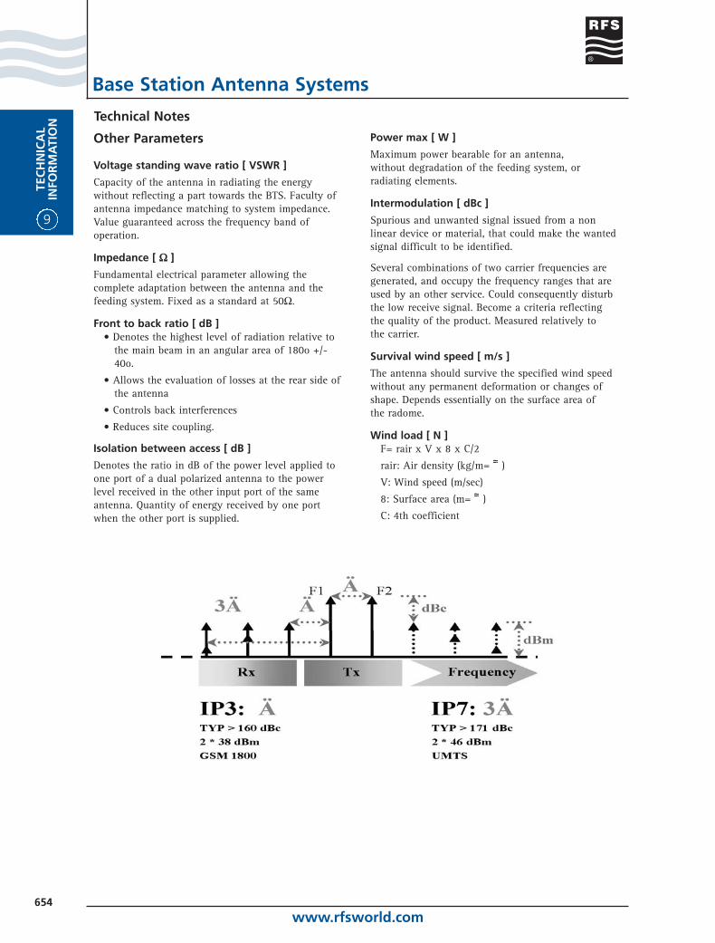
Intermodulation [ dBc ]

Spurious and unwanted signal issued from a nonlinear device or material, that could make the wantedsignal difficult to be identified.

Several combinations of two carrier frequencies aregenerated, and occupy the frequency ranges that areused by an other service. Could consequently disturbthe low receive signal. Become a criteria reflecting the quality of the product. Measured relatively to the carrier.

Survival wind speed [ m/s ]

The antenna should survive the specified wind speedwithout any permanent deformation or changes ofshape. Depends essentially on the surface area ofthe radome.

Wind load [ N ]F= rair x V x 8 x C/2

rair: Air density (kg/m= )

V: Wind speed (m/sec)

8: Surface area (m= )

C: 4th coefficient

Technical Notes

www.rfsworld.com655

TECH

NIC

AL

INFO

RM

ATIO

N

9

RF Conditioning

Technical NotesMore on attenuation

Attenuation is also power absorbed by the filter as anintentional benefit. It applies to band rejection, and isthe extent to which the undesirable signal is blockedfrom the filter’s output. This is a key parameter induplexers, whose task is to prevent transmitter powerfrom entering the receiver's input.

Some filters offer up to 100 dB or more attenuation, avery significant reduction in the unwanted signal. Forrepeater service, consult the radio manufacturer’s datasheet for recommended attenuation required.

Isolation

Isolation is the amount of attenuation between namedports of a filter. For example, a duplexer specified ashaving 80 dB of attenuation between the receiver portand the transmitter port may be said to have 80 dB port-to-port isolation.

Bandwidth

The amount of frequency spectrum within theinsertion loss points specified of a filter’s responsecurve is defined as the filter’s pass bandwidth. In mostcases this will be significantly less than the 3 dBbandwidth of the filter. If the filter has a complexresponse curve, there may be one or more passbandwidths and reject bandwidths associated with thedevice.

Selectivity

The shape of the filter’s response curve defines thefilter’s selectivity characteristics. Sharp curves withsteep “skirts” have relatively narrow bandwidths, andare considered highly selective. A relatively widebandwidth has broad selectivity. Each selectivityextreme has utility for a given set of circumstancesfacing the system designer.

Types of filters

Types of filters available to the designer include lowpass, high pass, band pass, and band reject filters.

Low pass filters attenuate radio frequency energyabove a certain cutoff point. In other words, they passlow. A typical use of a low pass filter involvessuppressing the unwanted second harmonic and othersabove it from a transmitter. For example, a transmitterdesigned for 27 MHz service will generate a secondharmonic at 54 MHz and, to a lesser extent, highermultiples. A good low pass filter will only permit the 27 mHz energy toreach the antenna, thus preventing interference withother radio services.

High pass filters attenuate radio frequency energybelow a certain cutoff point. These filters pass high.They are the electrical mirror image of low pass filters.

Filters

Filters are important passive RF devices that performselective frequency discrimination. As a class, filters also include duplexer and cavity resonators. Filters aredesigned to pass a band of frequencies, reject a band, or to combine those actions.

Four prime filter characteristics of concern to thesystem designer are insertion loss, attenuation,bandwidth, and selectivity. Each must be consideredcarefully in the selection of a filter product in order toensure satisfactory system performance.

Insertion loss and attenuation

Both represent reduction of available signal powerafter filtering. Generally speaking, the designer selectsthe filter with the least loss and the most attenuationconsistent with other application requirements.

Although one may discuss loss directly in terms ofWatts, it is common practice to use the Decibel toexpress the ratio of power output to power input. Using Decibels makes insertion loss and attenuationperformance characteristics independent of the actualpowers or voltages in use.

The Decibel (abbreviated dB, where the B is in honorof Alexander Graham Bell) is computed as 10log(Pout/Pin). where log is the common logarithmfunction (base 10). Pout is the measured output powerfrom the filter; Pin is the measure of power input to the filter. A fewuseful ratios and their corresponding Decibels aretabulated on the following chart.

Decibel Loss = Power Loss0.5 dB 10.8%

1.0 dB 20.5%

2.0 dB 36.9%

3.0 dB 50.5%

10.0 dB 90.0%

As may be seen from the table, the often-heardexpression “half-power point” signifies that spot on the response curve where the output power has beenreduced by 3 dB, regardless of the actual power level.

Insertion loss is the amount of power unavoidablyabsorbed by the filter. It’s an unintended side effect...a “cost of doing business” with the filter. In the bandpass region of the filter’s response curve, this figuresets the maximum amount of desired signal passedthrough to the output after processing. There arepractical lower limits on insertion loss, around 0.5 dB.A 3 dB insertion loss, for example, spends half yourpower in the filter. Sometimes a relatively highamount is unavoidable, as in transmitter combiners.

9

TEC

HN

ICA

LIN

FOR

MA

TIO

N

www.rfsworld.com656

diameter. Temperature compensation in helicalcavities is more difficult to control than with TEMcavities, so helical designs are not specified fornarrow bandwidth requirements.

Duplexers

These products are an integration of filter sections,generally cavity resonators, and are used predomi-nantly to facilitate duplex repeater operation utilizinga single antenna and feedline. Duplexers range in sizeand power handling capability from small mobiletypes to high-power base station units. They providethe critical isolation between receiver and transmitterthat allows both to be connected to the antennasimultaneously without the need for a transmit-receive relay.

A note of cautionThe cost and construction of duplexers varies with the transmit-receive frequency separation (offset)required, power handling capability, and ambient RF environmental constraints. For applications inwhich the offsets are relatively wide duplexers can be constructed using band pass filters. The inherentadvantage of this design is that unwanted signalrejection occurs for all frequencies outside theintended pass bands, not just at the duplexer’s

own transmit frequency. This duplexer design ispreferred for high ambient RF environments where it provides strong defense against unwanted signalsfrom nearby antennas.

Where the frequency offsets are closer (between about 0.5 MHz and 4.5 MHz) band reject cavities canbe used to build a duplexer. This cavity style offers the benefits of high isolation and low insertion loss,but the resulting duplexer generally lacks attenuationat frequencies other than the transmit and receivefrequencies specified. Consequently, this design should not be used where high ambient RF levels exist, unless other auxiliary filtering is considered.

Filter tuning

A good rule-of-thumb to remember when tuning anyRF filter of the types described above: Never tune theunit under full power. Always rely upon small-signalmethods using service monitors, frequency generators,calibrated receivers, etc. The reason: during the tune-up process, off-resonance conditions occur when the tuning screws are adjusted for their optimum setting. At resonance, the reactivecomponents increase sharply, as does thecorresponding voltage drop across insulating parts.High voltage drops may lead to arcing, which can leave permanent carbon traces across internalinsulating material. Leakage across these traces causes instability in the filter’s tuning, and noisyduplex operation. In designs employing moving finger stock for ground contact, arcing and pitting will occur when the finer stock position is changed in the presence of power, resulting in the same deteriorated performance. Damage of this nature is generally ruinous to the filter.

RF Conditioning

Technical NotesBand pass filters pass a band of frequencies betweenspecified low and high frequency cutoff points. RFenergy above and below these cutoff frequencies isattenuated. Bandpass filters find wide application inland- mobile communications work. A typicalapplication involves high power paging transmitters,where digital modulation tends to create adjacentchannel interference with nearby receivers. Use of aband pass-style filtering device (usually a cavityresonator) will “sharpen” the paging transmitter’s RFoutput spectrum, permitting only the energy in theimmediate vicinity of the carrier to be radiated fromthe antenna.

Band reject filters block, or “notch out” a band offrequencies between specified low and high frequencycutoff points. These devices are the electrical mirrorimage of band pass filters. RF energy below andabove the cutoff points is passed to the filter output.Band reject filters also find wide application in theland mobile industry. As in the paging transmitterexample, receivers with insufficient inherentselectivity that experience such interference can beoutfitted with a notch filter adjusted to the offendingtransmitters frequency, which effectively eliminatesthe interfering signal. Sometimes filters are requiredon both radios to completely solve interferenceproblems at a site.

Cavities

Resonant cavitiesSuccessful commercial products are usually based on one of three basic designs: helical, transverseelectromagnetic (TEM), and waveguide. In mostcommon use at this time are the helical and TEM styles.

TEM cavities TEM cavities are usually built as quarter- or three-quarter-wavelength resonators, with the long designused for low loss, high selectivity applications. The Q or quality factor of a TEM cavity increases as thediameter is increased to a limit point, depending upon the conductivity of the materials used in itsconstruction. Silver plating can be applied to improve the cavity’s Q.

Frequency stability of a TEM cavity can be preciselycontrolled by incorporating an invar rod for tuning the inner conductor. Invar, with its low coefficient of expansion vs. temperature, allows the cavity to be tuned over a wide range of frequencies while thelength of the tuning rod remains nearly constant over an extended range of ambient temperatures. RFS product designers take full advantage of all of these techniques to offer superior frequency stability performance.

Helical cavitiesHelical cavities have generally been designed for lowpower, low Q applications such as receiver front-endsand mobile duplexers. As with the TEM style, the Q ofthe helical type is proportionate to the cavity

www.rfsworld.com657

TECH

NIC

AL

INFO

RM

ATIO

N

9

UHF Television Systems Utilizing Panel Arrays

Introduction

This guide is issued by RFS as an aid for those peopleinvolved in the design of UHF TV transmittingsystems. It is based on the use of broadband panelarrays incorporating the PHP and PVP panels forhorizontal and vertical polarization respectively. Theguide is fully supported by our professional engineerswho are available to give advice as required.

The systems described herein cover 1 to 16 bayantennas. Large arrays almost always require specialengineering considerations which cannot beincorporated here, but the information provided isintended to cover the broader system aspects of panelarray design. Please consult our engineers for furtherinformation and assistance.

Electrical Considerations

Polarization

Horizontal Polarization:

The model PHP panel is horizontally polarized. Itcovers all of 470-860MHz.

Vertical Polarization:

The model PVP panel is vertically polarized and likethe PHP panel covers all of 470-860MHz.

Gain

All antenna systems considered here incorporate equalnumbers of panels on all faces.

For such systems the peak gain of the antenna is theproduct of the horizontal and vertical patterndirectives less any distribution losses incurred withinthe antenna feed system. Null fill loss is included inthe vertical directivity.

So in decibels the antenna peak gain is given by:

GAPK = GH + GV - LD dBd

where

GH = Horizontal pattern directivity (dB)GV = Vertical patter directivity (dB)LD = Distribution losses

For omni directional systems it is normal to considerthe RMS gain which is given by:

GARMS = GV - LD

The distribution losses for an antenna will varydepending on the size of the array and the type(s) of

distribution cables used. The latter is a function of thepower handling requirements for the system. Typically,the following figures can be used for low/mediumpower systems.

ANTENNA SIZE LOSS (DB)1-Bay 0.052-Bay 0.13-Bay 0.14-Bay 0.26-Bay 0.38-Bay 0.3

Antennas incorporating larger distribution feederand/or operating at lower frequencies will have lowerlosses than those described above. Higher poweredarrays larger than eight bays usually have losses ofapproximately 0.2dB.

Impedance and VSWR

For low and medium power arrays the input VSWR ofthe arrays will be better than 1.1:1 over approximately300 MHz bandwidth or greater.

For higher power arrays the VSWR will be better than1.05:1 on each vision carrier and better than 1.1:1 overeach operating channel. Other specifications tocustomer requirements are available.

Power Handling Capacity

Analog Services

The average power-handling requirement of an antennais the sum of the average input powers. The averagepower of a black level PAL TV picture with 10:1vision/sound ratio is 0.71 times the peak sync power.

The average power rating is a measure of the antennacapacity to dissipate the heat generated due to losses.

VPEAK = 1.4 divided by Ppeak x 50

For low and medium power arrays the average powerrating will be generally limited by the size of the inputpower divider as follows:

7/8" EIA: 2kW average1-5/8" EIA: 5kW average3-1/8" EIA: 12kW average4-1/2" IEC 36kW average6-1/8" EIA 55kW average

For high power arrays the average power rating can belimited by any part of the distribution system or thepanels and will vary depending on the configuration ofthe array. Input connectors are usually 4-1/2" IEC or 6-1/8" EIA. 7-3/16" EIA and larger inputs are availableon request.

Broadcast Antenna Systems

9

TEC

HN

ICA

LIN

FOR

MA

TIO

N

www.rfsworld.com658

The peak power rating is a measure of the voltagebreakdown or flashover point of the antenna. It iscommon to express peak power rating in terms of thepeak voltage rating. Generally the peak powerhandling capacity will not be a limiting factor in theantenna design, however it needs to be checkedespecially where there are a large number of inputchannels.

The peak power handling requirement of an antennawill be PPK = 1.4 n2 PAV where n = the number ofinput channels and PAV is the average power inputper channel where all channels are of the same power.

Digital Services

Because of the much higher peak to average powerratios of digital services the peak power ratings are farmore significant than for analog services. Digitalservices are rated using the peak power. The totalpower is the sum of the peak powers of the digitalservices.

System Losses

The system design must take account of lossesincurred by the main feed cable(s) and any internalplant equipment such as combiners and switch frames.

Feeder Losses

The attenuation figures for Heliflex flexible coaxialtransmission line can be found on the relevant specifi-cation pages of this catalog. This technicalinformation section also contains a good explanationof how the specifications are derived.

Combiner Losses

Combiner losses vary according to the type ofcombiner used, frequency spacings between channelstransmission line sizes utilized and the number ofchannels to be combined.

For the purposes of this guide it will be assumed thatthe frequency spacing is 3 channels and that betweentwo and six channels will be combined.

Two different constant impedance combining systemsare used: commutating line and balanced (bandpassfilter). The former is commonly used for 2, 3 or 4channel systems. The latter is used for any number ofchannels. The commutating line devices are lessexpensive however they generally have higher lossesespecially at close frequency spacing.

Typical Combiner Losses (per channel, 21 MHzspacing)

Commutating Line Combiner (CUC Series):

INPUT CONNECTOR N 1-5/8" 3-1/8" 4-1/8"2 channels Loss (dB) 0.7 0.4 0.3 0.253, 4 channels Loss (dB) 1.3 0.6 0.45 0.4

Bandpass Filter Combiner (CU Series):

INPUT CONNECTOR 1-5/8" 3-1/8"First Channel Loss (dB) 0.4 0.3Additional Channels Loss (dB) 0.1 0.1

Switch Frame Loss

If a switch frame is incorporated in the system allow0.1dB insertion loss.

Internal Rigid Line Loss

Allowance should be made for any internal rigid line(or jumper cables) between the transmitter and anyswitch frames, combiners and main feed cables.

Rigid line losses are as follows.

LINE SIZE 1-5/8" 3-1/8" 4-1/8"Loss dB/100m at 500 MHz 1.6 0.8 0.55Loss dB/100m at 800 MHz 1.95 1.0 0.70

Typical Performance Summary

An example of a system performance summary of an8 channel directional system as shown in the tablebelow for a low power site. (only 3 of the 8 channelsare included). The antenna directivity shown is thesum of the horizontal and vertical pattern directivities.

Typical System Performance Summary

FREQUENCY, MHZ 813-820 750-757 547-554Antenna Directivity, dBd 15.9 16.8 17.4Antenna Losses, dB 0.3 0.3 0.3Feeder Loss (50m of HF 1-5/8"), dB 0.95 0.90 0.75Combiner Loss, dB 0.5 0.8 0.9U Link panel and rigid line loss, dB 0.2 0.2 0.210m of HF 7/8" internal feeder, dB 0.35 0.33 0.28System Peak Gain, dBd 13.6 14.3 15.0Peak ERP (5kW), kW 5.0 5.0 5.0Tx Power, Watts 218 187 159

UHF Television Systems Utilizing Panel Arrays

Broadcast Antenna Systems

www.rfsworld.com659

TECH

NIC

AL

INFO

RM

ATIO

N

9

Mechanical Considerations

Support Columns

Standard support columns are available for 1 to 16-bay systems for both cantilever and side-mounting.They are made of hot dipped galvanized steel.

Columns up to eight levels are provided as a singlepiece. Six and eight level columns may be provided asan option in two modules to facilitate ease oftransport and installation. Columns above eight levelsare always provided in modules.

Small arrays can be pole mounted.

Ladders

On cantilever columns external ladders can beprovided to allow external access to the antenna forhorizontally polarized systems. For vertically polarizedsystems climbing spikes are available. Internal laddersare usually incorporated into all columns.

Pressurization

All feed systems are pressure-tight to the panel inputs.It is strongly recommended that these systems bepressurized with dry air to inhibit the ingress ofmoisture. Pressure is supplied via the main feed cable.Recommended operating pressure is in the range 20-35kPa.

All pressure-tight components are tested in the factoryat 70kPa. The entire antenna system is also pressure-tested.

Lightning Protection

Cantilever columns are provided with one or two 1.5mlong lightning spikes. The antenna system is firmlybonded to the column. On installation it is importantthat the column is solidly bonded to the supportstructure.

Shipping

Up to eight bay arrays are shipped fully assembledunless modular antenna systems are requested.Antennas are supported on steel frames for shipment.

Interface and Tower Design Considerations

As well as designing a tower capable of accommo-dating the weight and wind loading of the column,the physical deflection of the tower must also belimited. This is necessary because of the very narrowbeam in the vertical plane. Excessive tower deflectionmay cause TV pictures to flutter as the signal in theviewer's direction fluctuates from the main beam tothe nulls on either side in the vertical plane.

A deflection of 3/8 wavelengths (139mm at 800 MHz)is a reasonable limit for the top of the antenna at theserviceability wind speed.

The main feeder cable may be a significant weight (6-1/8" feeder weighs approximately 11kg/m) and it mustbe protected so it is recommended that the towerincorporates a vertical cable runway inside the tower,usually alongside the ladder.

Access is required at the base of the antenna columnto commission the antenna and it is recommendedthat a maintenance platform be situated approxi-mately 1.5 - 2m below the base of the antenna.

Installation Considerations

Care should be taken during the lifting operation toensure that the feeder or antenna is not damaged.

Once the antenna has been installed it should bepurged with dry air for a minimum of 6 hours toensure that all moisture is removed. Consult theantenna handbook for the correct purging procedure.

If the antenna has dual inputs it will be necessary toequalize the main feeder cables to ensure eachantenna stack is fed with the correct phase.

UHF Television Systems Utilizing Panel Arrays

Broadcast Antenna Systems

9

TEC

HN

ICA

LIN

FOR

MA

TIO

N

www.rfsworld.com660

Broadcast Antenna SystemsBalanced Combiner Modules

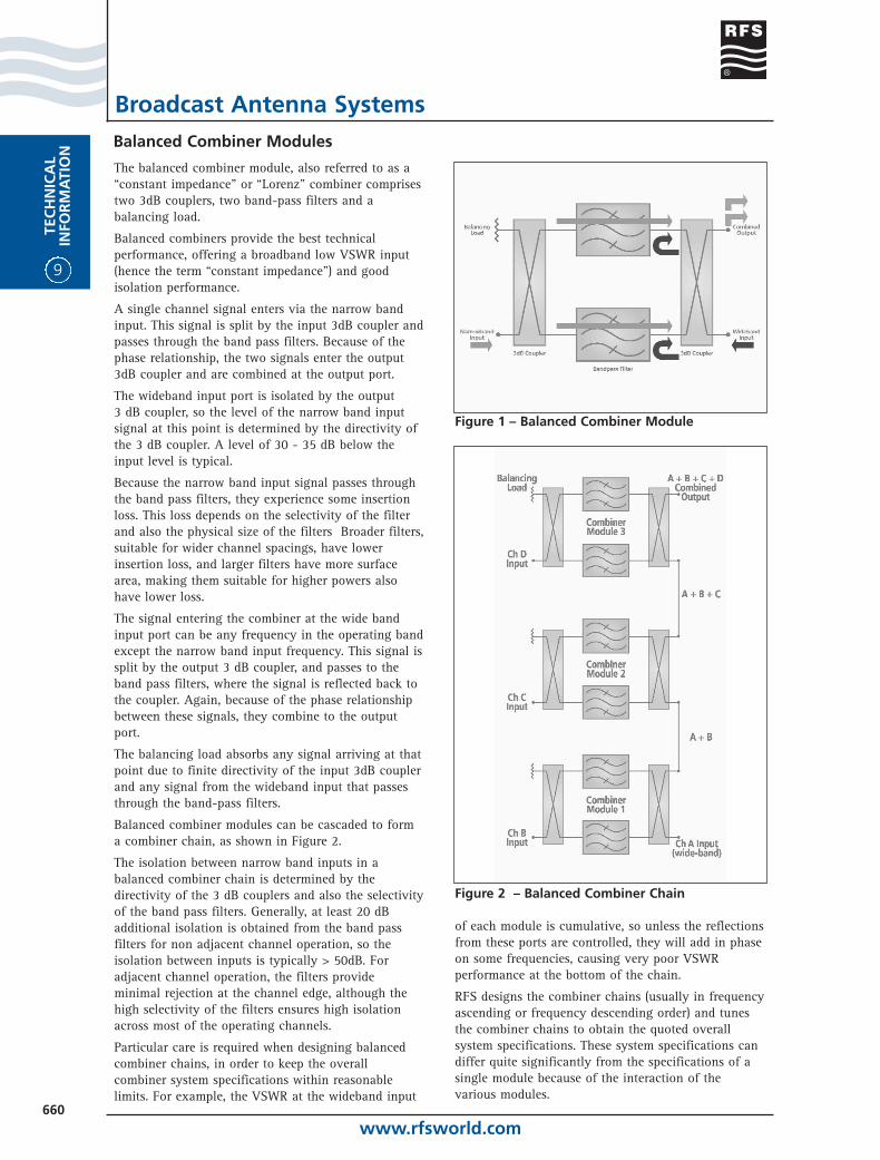
The balanced combiner module, also referred to as a“constant impedance" or “Lorenz" combiner comprisestwo 3dB couplers, two band-pass filters and abalancing load.

Balanced combiners provide the best technicalperformance, offering a broadband low VSWR input(hence the term “constant impedance") and goodisolation performance.

A single channel signal enters via the narrow bandinput. This signal is split by the input 3dB coupler andpasses through the band pass filters. Because of thephase relationship, the two signals enter the output3dB coupler and are combined at the output port.

The wideband input port is isolated by the output 3 dB coupler, so the level of the narrow band inputsignal at this point is determined by the directivity ofthe 3 dB coupler. A level of 30 - 35 dB below theinput level is typical.

Because the narrow band input signal passes throughthe band pass filters, they experience some insertionloss. This loss depends on the selectivity of the filterand also the physical size of the filters Broader filters,suitable for wider channel spacings, have lowerinsertion loss, and larger filters have more surfacearea, making them suitable for higher powers alsohave lower loss.

The signal entering the combiner at the wide bandinput port can be any frequency in the operating bandexcept the narrow band input frequency. This signal issplit by the output 3 dB coupler, and passes to theband pass filters, where the signal is reflected back tothe coupler. Again, because of the phase relationshipbetween these signals, they combine to the outputport.

The balancing load absorbs any signal arriving at thatpoint due to finite directivity of the input 3dB couplerand any signal from the wideband input that passesthrough the band-pass filters.

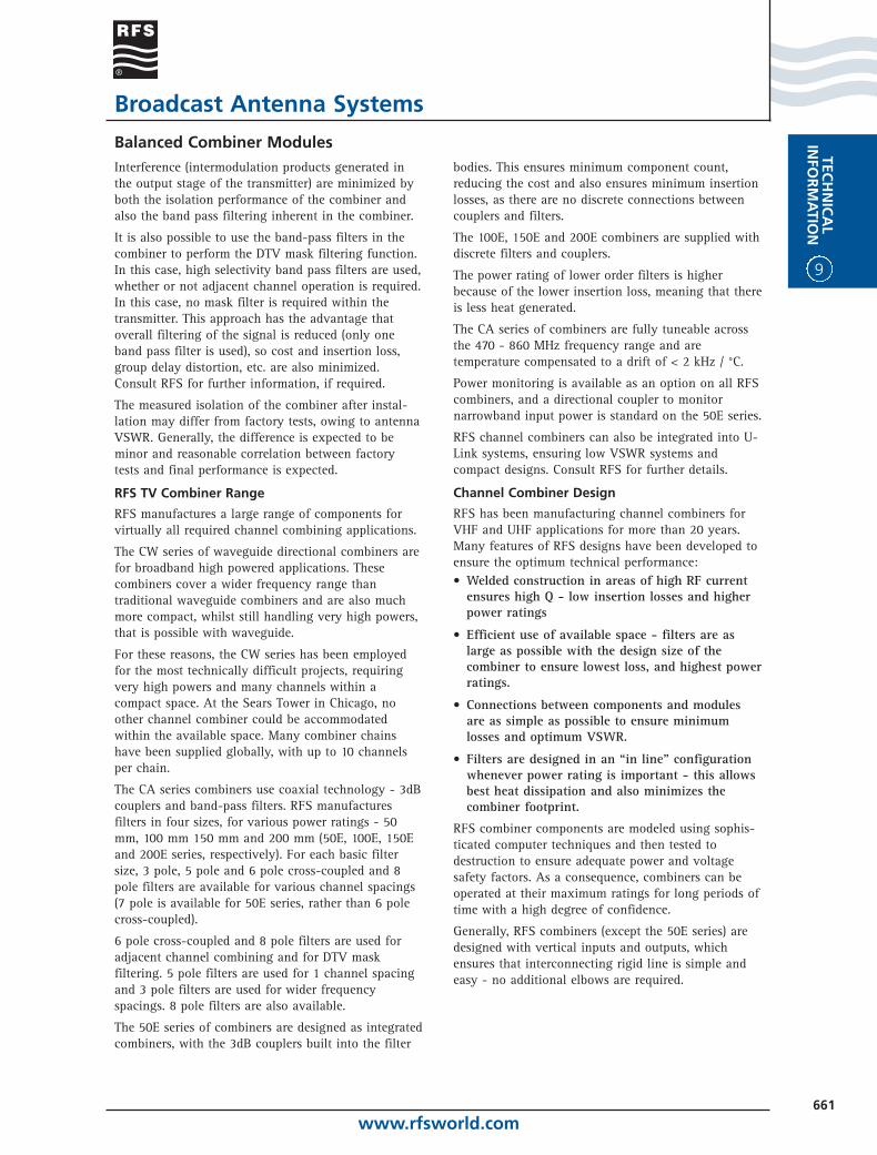
Balanced combiner modules can be cascaded to forma combiner chain, as shown in Figure 2.

The isolation between narrow band inputs in abalanced combiner chain is determined by thedirectivity of the 3 dB couplers and also the selectivityof the band pass filters. Generally, at least 20 dBadditional isolation is obtained from the band passfilters for non adjacent channel operation, so theisolation between inputs is typically > 50dB. Foradjacent channel operation, the filters provideminimal rejection at the channel edge, although thehigh selectivity of the filters ensures high isolationacross most of the operating channels.

Particular care is required when designing balancedcombiner chains, in order to keep the overallcombiner system specifications within reasonablelimits. For example, the VSWR at the wideband input

Figure 1 – Balanced Combiner Module

Figure 2 – Balanced Combiner Chain

of each module is cumulative, so unless the reflectionsfrom these ports are controlled, they will add in phaseon some frequencies, causing very poor VSWRperformance at the bottom of the chain.

RFS designs the combiner chains (usually in frequencyascending or frequency descending order) and tunesthe combiner chains to obtain the quoted overallsystem specifications. These system specifications candiffer quite significantly from the specifications of asingle module because of the interaction of thevarious modules.

www.rfsworld.com661

TECH

NIC

AL

INFO

RM

ATIO

N

9

Balanced Combiner ModulesInterference (intermodulation products generated inthe output stage of the transmitter) are minimized byboth the isolation performance of the combiner andalso the band pass filtering inherent in the combiner.

It is also possible to use the band-pass filters in thecombiner to perform the DTV mask filtering function.In this case, high selectivity band pass filters are used,whether or not adjacent channel operation is required.In this case, no mask filter is required within thetransmitter. This approach has the advantage thatoverall filtering of the signal is reduced (only oneband pass filter is used), so cost and insertion loss,group delay distortion, etc. are also minimized.Consult RFS for further information, if required.

The measured isolation of the combiner after instal-lation may differ from factory tests, owing to antennaVSWR. Generally, the difference is expected to beminor and reasonable correlation between factorytests and final performance is expected.

RFS TV Combiner Range

RFS manufactures a large range of components forvirtually all required channel combining applications.

The CW series of waveguide directional combiners arefor broadband high powered applications. Thesecombiners cover a wider frequency range thantraditional waveguide combiners and are also muchmore compact, whilst still handling very high powers,that is possible with waveguide.

For these reasons, the CW series has been employedfor the most technically difficult projects, requiringvery high powers and many channels within acompact space. At the Sears Tower in Chicago, noother channel combiner could be accommodatedwithin the available space. Many combiner chainshave been supplied globally, with up to 10 channelsper chain.

The CA series combiners use coaxial technology - 3dBcouplers and band-pass filters. RFS manufacturesfilters in four sizes, for various power ratings - 50mm, 100 mm 150 mm and 200 mm (50E, 100E, 150Eand 200E series, respectively). For each basic filtersize, 3 pole, 5 pole and 6 pole cross-coupled and 8pole filters are available for various channel spacings(7 pole is available for 50E series, rather than 6 polecross-coupled).

6 pole cross-coupled and 8 pole filters are used foradjacent channel combining and for DTV maskfiltering. 5 pole filters are used for 1 channel spacingand 3 pole filters are used for wider frequencyspacings. 8 pole filters are also available.

The 50E series of combiners are designed as integratedcombiners, with the 3dB couplers built into the filter

bodies. This ensures minimum component count,reducing the cost and also ensures minimum insertionlosses, as there are no discrete connections betweencouplers and filters.

The 100E, 150E and 200E combiners are supplied withdiscrete filters and couplers.

The power rating of lower order filters is higherbecause of the lower insertion loss, meaning that thereis less heat generated.

The CA series of combiners are fully tuneable acrossthe 470 - 860 MHz frequency range and aretemperature compensated to a drift of < 2 kHz / °C.

Power monitoring is available as an option on all RFScombiners, and a directional coupler to monitornarrowband input power is standard on the 50E series.

RFS channel combiners can also be integrated into U-Link systems, ensuring low VSWR systems andcompact designs. Consult RFS for further details.

Channel Combiner Design

RFS has been manufacturing channel combiners forVHF and UHF applications for more than 20 years.Many features of RFS designs have been developed toensure the optimum technical performance:• Welded construction in areas of high RF current

ensures high Q - low insertion losses and higherpower ratings

• Efficient use of available space - filters are aslarge as possible with the design size of thecombiner to ensure lowest loss, and highest powerratings.

• Connections between components and modulesare as simple as possible to ensure minimumlosses and optimum VSWR.

• Filters are designed in an “in line" configurationwhenever power rating is important - this allowsbest heat dissipation and also minimizes thecombiner footprint.

RFS combiner components are modeled using sophis-ticated computer techniques and then tested todestruction to ensure adequate power and voltagesafety factors. As a consequence, combiners can beoperated at their maximum ratings for long periods oftime with a high degree of confidence.

Generally, RFS combiners (except the 50E series) aredesigned with vertical inputs and outputs, whichensures that interconnecting rigid line is simple andeasy - no additional elbows are required.

Broadcast Antenna Systems

9

TEC

HN

ICA

LIN

FOR

MA

TIO

N

www.rfsworld.com662

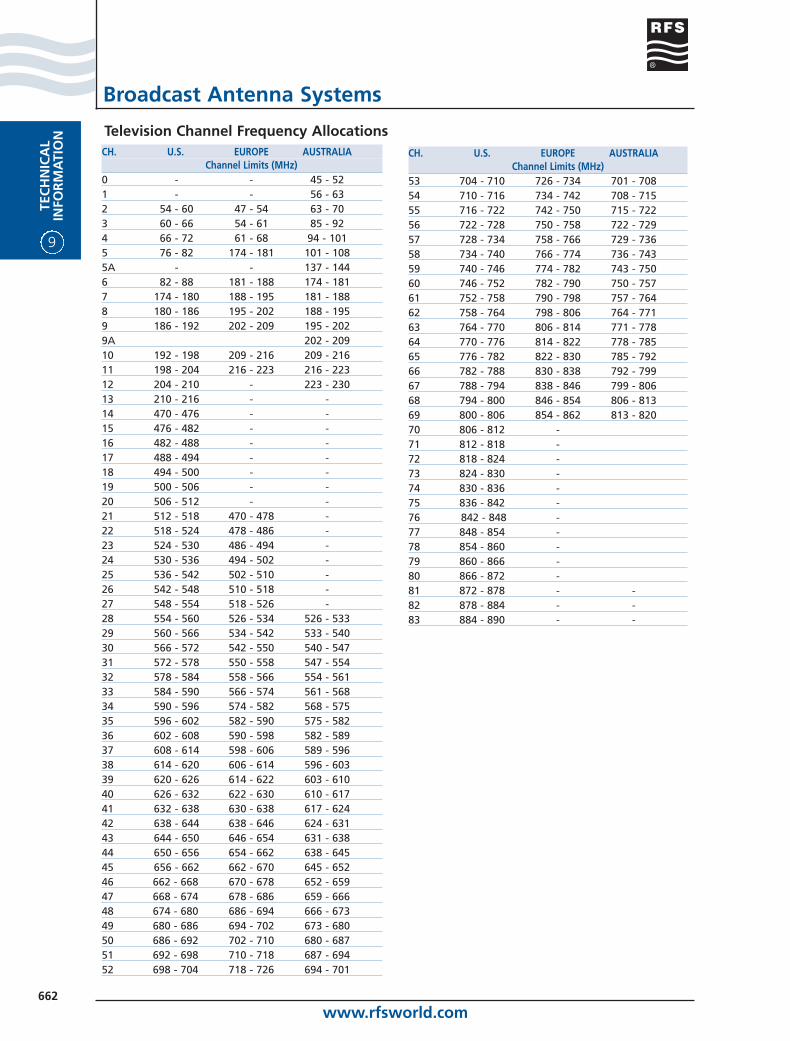
Television Channel Frequency Allocations

Broadcast Antenna Systems

CH. U.S. EUROPE AUSTRALIAChannel Limits (MHz)

53 704 - 710 726 - 734 701 - 70854 710 - 716 734 - 742 708 - 71555 716 - 722 742 - 750 715 - 72256 722 - 728 750 - 758 722 - 72957 728 - 734 758 - 766 729 - 73658 734 - 740 766 - 774 736 - 74359 740 - 746 774 - 782 743 - 75060 746 - 752 782 - 790 750 - 75761 752 - 758 790 - 798 757 - 76462 758 - 764 798 - 806 764 - 77163 764 - 770 806 - 814 771 - 77864 770 - 776 814 - 822 778 - 78565 776 - 782 822 - 830 785 - 79266 782 - 788 830 - 838 792 - 79967 788 - 794 838 - 846 799 - 80668 794 - 800 846 - 854 806 - 81369 800 - 806 854 - 862 813 - 82070 806 - 812 -71 812 - 818 -72 818 - 824 -73 824 - 830 -74 830 - 836 -75 836 - 842 -76 842 - 848 -77 848 - 854 -78 854 - 860 -79 860 - 866 -80 866 - 872 -81 872 - 878 - -82 878 - 884 - -83 884 - 890 - -

CH. U.S. EUROPE AUSTRALIAChannel Limits (MHz)

0 - - 45 - 521 - - 56 - 632 54 - 60 47 - 54 63 - 703 60 - 66 54 - 61 85 - 924 66 - 72 61 - 68 94 - 1015 76 - 82 174 - 181 101 - 1085A - - 137 - 1446 82 - 88 181 - 188 174 - 1817 174 - 180 188 - 195 181 - 1888 180 - 186 195 - 202 188 - 1959 186 - 192 202 - 209 195 - 2029A 202 - 20910 192 - 198 209 - 216 209 - 21611 198 - 204 216 - 223 216 - 22312 204 - 210 - 223 - 23013 210 - 216 - -14 470 - 476 - -15 476 - 482 - -16 482 - 488 - -17 488 - 494 - -18 494 - 500 - -19 500 - 506 - -20 506 - 512 - -21 512 - 518 470 - 478 -22 518 - 524 478 - 486 -23 524 - 530 486 - 494 -24 530 - 536 494 - 502 -25 536 - 542 502 - 510 -26 542 - 548 510 - 518 -27 548 - 554 518 - 526 -28 554 - 560 526 - 534 526 - 53329 560 - 566 534 - 542 533 - 54030 566 - 572 542 - 550 540 - 54731 572 - 578 550 - 558 547 - 55432 578 - 584 558 - 566 554 - 56133 584 - 590 566 - 574 561 - 56834 590 - 596 574 - 582 568 - 57535 596 - 602 582 - 590 575 - 58236 602 - 608 590 - 598 582 - 58937 608 - 614 598 - 606 589 - 59638 614 - 620 606 - 614 596 - 60339 620 - 626 614 - 622 603 - 61040 626 - 632 622 - 630 610 - 61741 632 - 638 630 - 638 617 - 62442 638 - 644 638 - 646 624 - 63143 644 - 650 646 - 654 631 - 63844 650 - 656 654 - 662 638 - 64545 656 - 662 662 - 670 645 - 65246 662 - 668 670 - 678 652 - 65947 668 - 674 678 - 686 659 - 66648 674 - 680 686 - 694 666 - 67349 680 - 686 694 - 702 673 - 68050 686 - 692 702 - 710 680 - 68751 692 - 698 710 - 718 687 - 69452 698 - 704 718 - 726 694 - 701

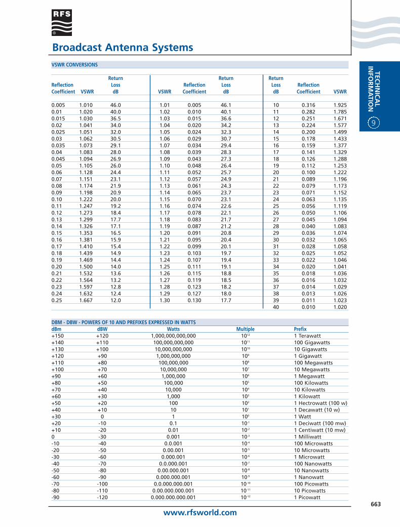
www.rfsworld.com663

TECH

NIC

AL

INFO

RM

ATIO

N

9

Broadcast Antenna SystemsVSWR CONVERSIONS

Return Return ReturnReflection Loss Reflection Loss Loss ReflectionCoefficient VSWR dB VSWR Coefficient dB dB Coefficient VSWR

0.005 1.010 46.0 1.01 0.005 46.1 10 0.316 1.9250.01 1.020 40.0 1.02 0.010 40.1 11 0.282 1.7850.015 1.030 36.5 1.03 0.015 36.6 12 0.251 1.6710.02 1.041 34.0 1.04 0.020 34.2 13 0.224 1.5770.025 1.051 32.0 1.05 0.024 32.3 14 0.200 1.4990.03 1.062 30.5 1.06 0.029 30.7 15 0.178 1.4330.035 1.073 29.1 1.07 0.034 29.4 16 0.159 1.3770.04 1.083 28.0 1.08 0.039 28.3 17 0.141 1.3290.045 1.094 26.9 1.09 0.043 27.3 18 0.126 1.2880.05 1.105 26.0 1.10 0.048 26.4 19 0.112 1.2530.06 1.128 24.4 1.11 0.052 25.7 20 0.100 1.2220.07 1.151 23.1 1.12 0.057 24.9 21 0.089 1.1960.08 1.174 21.9 1.13 0.061 24.3 22 0.079 1.1730.09 1.198 20.9 1.14 0.065 23.7 23 0.071 1.1520.10 1.222 20.0 1.15 0.070 23.1 24 0.063 1.1350.11 1.247 19.2 1.16 0.074 22.6 25 0.056 1.1190.12 1.273 18.4 1.17 0.078 22.1 26 0.050 1.1060.13 1.299 17.7 1.18 0.083 21.7 27 0.045 1.0940.14 1.326 17.1 1.19 0.087 21.2 28 0.040 1.0830.15 1.353 16.5 1.20 0.091 20.8 29 0.036 1.0740.16 1.381 15.9 1.21 0.095 20.4 30 0.032 1.0650.17 1.410 15.4 1.22 0.099 20.1 31 0.028 1.0580.18 1.439 14.9 1.23 0.103 19.7 32 0.025 1.0520.19 1.469 14.4 1.24 0.107 19.4 33 0.022 1.0460.20 1.500 14.0 1.25 0.111 19.1 34 0.020 1.0410.21 1.532 13.6 1.26 0.115 18.8 35 0.018 1.0360.22 1.564 13.2 1.27 0.119 18.5 36 0.016 1.0320.23 1.597 12.8 1.28 0.123 18.2 37 0.014 1.0290.24 1.632 12.4 1.29 0.127 18.0 38 0.013 1.0260.25 1.667 12.0 1.30 0.130 17.7 39 0.011 1.023

40 0.010 1.020

DBM - DBW - POWERS OF 10 AND PREFIXES EXPRESSED IN WATTSdBm dBW Watts Multiple Prefix+150 +120 1,000,000,000,000 1012 1 Terawatt+140 +110 100,000,000,000 1011 100 Gigawatts+130 +100 10,000,000,000 1010 10 Gigawatts+120 +90 1,000,000,000 109 1 Gigawatt+110 +80 100,000,000 108 100 Megawatts+100 +70 10,000,000 107 10 Megawatts+90 +60 1,000,000 106 1 Megawatt+80 +50 100,000 105 100 Kilowatts+70 +40 10,000 104 10 Kilowatts+60 +30 1,000 103 1 Kilowatt+50 +20 100 102 1 Hectrowatt (100 w)+40 +10 10 101 1 Decawatt (10 w)+30 0 1 100 1 Watt+20 -10 0.1 10-1 1 Deciwatt (100 mw)+10 -20 0.01 10-2 1 Centiwatt (10 mw)0 -30 0.001 10-3 1 Milliwatt-10 -40 0.0.001 10-4 100 Microwatts-20 -50 0.00.001 10-5 10 Microwatts-30 -60 0.000.001 10-6 1 Microwatt-40 -70 0.0.000.001 10-7 100 Nanowatts-50 -80 0.00.000.001 10-8 10 Nanowatts-60 -90 0.000.000.001 10-9 1 Nanowatt-70 -100 0.0.000.000.001 10-10 100 Picowatts-80 -110 0.00.000.000.001 10-11 10 Picowatts-90 -120 0.000.000.000.001 10-12 1 Picowatt

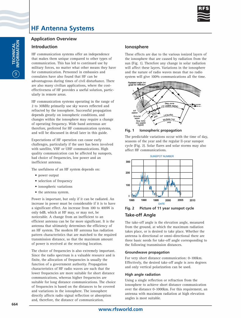
9

TEC

HN

ICA

LIN

FOR

MA

TIO

N

www.rfsworld.com664

Application Overview

HF Antenna Systems

Introduction

HF communication systems offer an independencethat makes them unique compared to other types ofcommunication. This has led to continued use bymilitary forces, no matter what other means they havefor communication. Personnel in embassies andconsulates have also found that HF can beadvantageous during times of civil disturbance. Thereare also many civilian applications, where the cost-effectiveness of HF provides a useful solution, partic-ularly in remote areas.

HF communication systems operating in the range of2 to 30MHz primarily use sky waves reflected andrefracted by the ionosphere. Successful propagationdepends greatly on ionospheric conditions, andchanges within the ionosphere may require a changeof operating frequency. Wide band antennas aretherefore, preferred for HF communication systems,and will be discussed in detail later in this guide.

Expectations of HF operation can cause earlychallenges, particularly if the user has been involvedwith satellite, VHF or UHF communications. Highquality communication can be affected by sunspots,bad choice of frequencies, low power and aninefficient antenna.

The usefulness of an HF system depends on:

• power output

• selection of frequency

• ionospheric variations

• the antenna system.

Power is important, but only if it can be radiated. Anincrease in power must be considerable if it is to havea significant effect. An increase from 100 to 400W isonly 6dB, which at HF may, or may not, benoticeable. A change from an inefficient to anefficient antenna can be far more significant. It is theantenna that ultimately determines the efficiency ofan HF system. The modern HF antenna has radiationpattern characteristics that are matched to the requiredtransmission distance, so that the maximum amountof power is received at the receiving location.

The choice of frequencies is also extremely important.Since the radio spectrum is a valuable resource and isfinite, the allocation of frequencies is usually thefunction of a government authority. Propagationcharacteristics of HF radio waves are such that thelower frequencies are more suitable for short distancecommunications, whereas higher frequencies aresuitable for long distance communications. The choiceof frequencies is based on the distances to be coveredand variations in the ionosphere. The ionospheredirectly affects radio signal reflection or absorptionand, therefore, the distance of communication.

Ionosphere

These effects are due to the various ionized layers ofthe ionosphere that are caused by radiation from thesun (Fig. 1). Therefore any change in solar radiationwill affect these layers. Variations in the ionosphereand the nature of radio waves mean that no radiosystem will give 100% communications all the time.

Fig. 1 Ionospheric propagation

The predictable variations occur with the time of day,seasons of the year and the regular ll-year sunspotcycle (Fig. 2). Solar flares and solar storms may alsoaffect HF communications.

Fig. 2 Picture of 11 year sunspot cycle

Take-off Angle

The take-off angle is the elevation angle, measuredfrom the ground, at which the maximum radiationtakes place, or is desired to take place. Whether theantenna is directional or omni-directional there arethree basic needs for take-off angle corresponding tothe following transmission distances.

Groundwave propagation

For very short distance communication: 0-100km.Effectively, the desired take-off angle is zero degreesand only vertical polarization can be used.

High angle radiation

Using a single reflection or refraction from theionosphere to achieve short distance communicationover the distance 0-1000km. For this requirement, anantenna with maximum radiation at high elevationangles is most suitable.

19951995 19901990 19951995 20002000 20052005 20102010

0

100100

200200

300300

DATE

SUNSPOT NUMBER

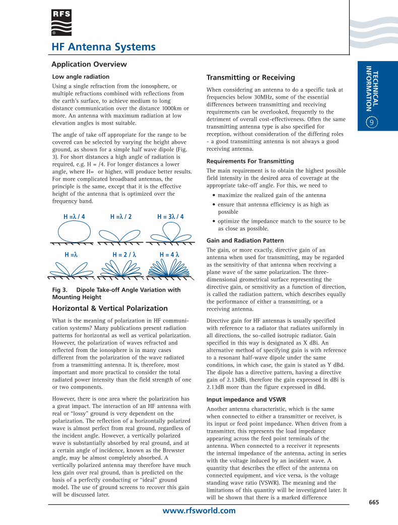
www.rfsworld.com665

TECH

NIC

AL

INFO

RM

ATIO

N

9

Application Overview

HF Antenna Systems

Low angle radiation

Using a single refraction from the ionosphere, ormultiple refractions combined with reflections fromthe earth’s surface, to achieve medium to longdistance communication over the distance 1000km ormore. An antenna with maximum radiation at lowelevation angles is most suitable.

The angle of take off appropriate for the range to becovered can be selected by varying the height aboveground, as shown for a simple half wave dipole (Fig.3). For short distances a high angle of radiation isrequired, e.g. H = /4. For longer distances a lowerangle, where H= or higher, will produce better results.For more complicated broadband antennas, theprinciple is the same, except that it is the effectiveheight of the antenna that is optimized over thefrequency band.

Fig 3. Dipole Take-off Angle Variation withMounting Height

Horizontal & Vertical Polarization

What is the meaning of polarization in HF communi-cation systems? Many publications present radiationpatterns for horizontal as well as vertical polarization.However, the polarization of waves refracted andreflected from the ionosphere is in many casesdifferent from the polarization of the wave radiatedfrom a transmitting antenna. It is, therefore, mostimportant and more practical to consider the totalradiated power intensity than the field strength of oneor two components.

However, there is one area where the polarization hasa great impact. The interaction of an HF antenna withreal or “lossy” ground is very dependent on thepolarization. The reflection of a horizontally polarizedwave is almost perfect from real ground, regardless ofthe incident angle. However, a vertically polarizedwave is substantially absorbed by real ground, and ata certain angle of incidence, known as the Brewsterangle, may be almost completely absorbed. Avertically polarized antenna may therefore have muchless gain over real ground, than is predicted on thebasis of a perfectly conducting or “ideal” groundmodel. The use of ground screens to recover this gainwill be discussed later.

Transmitting or Receiving

When considering an antenna to do a specific task atfrequencies below 30MHz, some of the essentialdifferences between transmitting and receivingrequirements can be overlooked, frequently to thedetriment of overall cost-effectiveness. Often the sametransmitting antenna type is also specified forreception, without consideration of the differing roles- a good transmitting antenna is not always a goodreceiving antenna.

Requirements For Transmitting

The main requirement is to obtain the highest possiblefield intensity in the desired area of coverage at theappropriate take-off angle. For this, we need to

• maximize the realized gain of the antenna

• ensure that antenna efficiency is as high aspossible

• optimize the impedance match to the source to beas close as possible.

Gain and Radiation Pattern

The gain, or more exactly, directive gain of anantenna when used for transmitting, may be regardedas the sensitivity of that antenna when receiving aplane wave of the same polarization. The three-dimensional geometrical surface representing thedirective gain, or sensitivity as a function of direction,is called the radiation pattern, which describes equallythe performance of either a transmitting, or areceiving antenna.

Directive gain for HF antennas is usually specifiedwith reference to a radiator that radiates uniformly inall directions, the so-called isotropic radiator. Gainspecified in this way is designated as X dBi. Analternative method of specifying gain is with referenceto a resonant half-wave dipole under the sameconditions, in which case, the gain is stated as Y dBd.The dipole has a directive pattern, having a directivegain of 2.13dBi, therefore the gain expressed in dBi is2.13dB more than the figure expressed in dBd.

Input impedance and VSWR

Another antenna characteristic, which is the samewhen connected to either a transmitter or receiver, isits input or feed point impedance. When driven from atransmitter, this represents the load impedanceappearing across the feed point terminals of theantenna. When connected to a receiver it representsthe internal impedance of the antenna, acting in serieswith the voltage induced by an incident wave. Aquantity that describes the effect of the antenna onconnected equipment, and vice versa, is the voltagestanding wave ratio (VSWR). The meaning and thelimitations of this quantity will be investigated later. Itwill be shown that there is a marked difference

H =ll / 4 H =ll / 2 H = 3ll / 4

H =ll H = 2 / ll H = 4 ll

9

TEC

HN

ICA

LIN

FOR

MA

TIO

N

www.rfsworld.com666

Application Overview

HF Antenna Systems

between the transmitting and receiving operation ofan antenna, and that the VSWR assumes differentsignificance, when considered for transmit or receiveantennas.

Fig. 4 Radio Transmission System

Fig. 4 shows a schematic circuit diagram of a typicalradio transmission system. The power of a transmitteris usually delivered to an antenna by means of atransmission line, in the frequency bands underconsideration. TX designates the transmitter operatinginto a load impedance ZT. TL is the transmission lineof characteristic impedance Z0, feeding the outputpower of the transmitter to the transmit antenna viathe coupling network CN, which transforms theantenna input impedance Z0 into ZL, the terminatingor load impedance of the transmission line.

Some antennas have been developed to match directlyto suitable transmission lines. The coupling networkCN, Fig. 4, is then unnecessary, and the antennaterminals are directly connected to the transmissionline. Examples include:

• Wideband HF conical vertical monopoles with atypical unbalanced input impedance of 50 ohms.

• Wideband HF biconical horizontal dipoles, with atypical balanced input impedance of 300 ohmsallowing direct connection to 300 ohm balancedline.

• Wideband HF vertical or horizontal HF log-periodic dipole antennas, also designed for 300ohm balanced line.

The wide-band properties of these antennas makethem very useful for transmitting stations. Although itis practically not possible to obtain a constantresistive antenna input impedance over the wantedwide frequency band, the designer keeps the fluctu-ations of the antenna input impedance ZA withrespect to Z0, the characteristic impedance of the line,within specified limits. A departure of ZA from Z0produces a partial reflection of the electromagneticpower from the antenna feed point thus producingstanding waves along the feeder line TL.

The standing waves are characterized by the “voltagestanding-wave-ratio (VSWR), which is the ratio of themaximum voltage on the line to the minimumvoltage. The transmitter is adjusted for optimumoperation when the line, TL in Fig. 4, is terminated ina resistive load equal to Z0. The power delivered tothis load is the practically obtainable maximum. If theline feeds the antenna and ZA differs from Z0, a part

of the power will be reflected back towards thetransmitter and the antenna radiated power is reduced,correspondingly, loss on the transmission lineincreases when VSWR rises. In a high powertransmitting system corona effects can occur on theline due to high VSWR.

A practical characteristic of a transmit antenna is themaximum permissible VSWR, which may bedesignated by SA. A frequently specified maximumVSWR, for antennas in the HF and MF bands is 2:1(i.e. SA = 2). This means that the mis-match betweenantenna impedance ZA and characteristic impedanceZ0 of the line reflects {(SA-1) / (SA+1)}2 x 100% =11% of the power and the signal strength is reducedby 0.5dB.

Coupling Networks

A more general problem is encountered when anantenna is used which has a nominal impedance ZCdifferent from the characteristic impedance Z0 of theselected transmission line. A coupling network CN willthen be inserted between antenna and line, as in Fig.4. The maximum VSWR of the antenna in theoperating frequency range, with respect to a line ofcharacteristic impedance ZC, may be designated bySC. The coupling network, designed for transfer of aterminating impedance ZC, into an input impedanceZL = Z0, will exhibit some fluctuations of the inputImpedance ZL due to variations in its frequencyresponse. The maximum VSWR appearing on the Z0line when the network CN is terminated by a resistiveimpedance ZC, may be designated by SC.

If a coupling network is used with the antenna, asshown in Fig. 4, the standing waves produced on thetransmission line TL will depend on the frequencyresponse of the antenna and the coupling network.The corresponding VSWR on the line TL may bedesignated by S0. Its value will be between limitsgiven by the inequality:

SASC S0 SA/SC, when SA > SC (If SA < SC, the lastterm has to be inverted).

Antenna Efficiency

The output power of the transmitter, reduced by theloss on the transmission line and in networks insertedbetween transmitter and antenna, represents the inputpower PA to the antenna. A part of this input powermay be dissipated in conductors and dielectriccomponents of the antenna and in the environment.e.g. in a ground system. The remaining power

P = hPA (h£1) is radiated

The antenna efficiency depends on the frequency, thetype of the antenna and on the environment.Theefficiency can be improved in certain cases, e.g. byimproving the ground system to reduce losses. Many

TX

ZO

TLZT

CNZL ZA

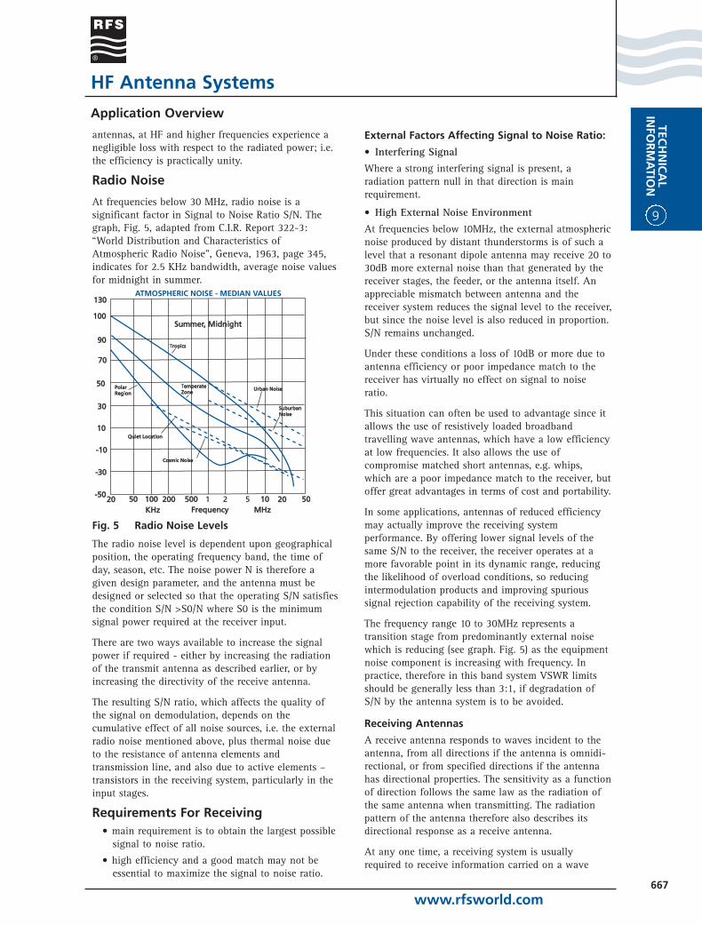
www.rfsworld.com667

TECH

NIC

AL

INFO

RM

ATIO

N

9

Application Overview

HF Antenna Systems

antennas, at HF and higher frequencies experience anegligible loss with respect to the radiated power; i.e.the efficiency is practically unity.

Radio Noise

At frequencies below 30 MHz, radio noise is asignificant factor in Signal to Noise Ratio S/N. Thegraph, Fig. 5, adapted from C.I.R. Report 322-3:“World Distribution and Characteristics ofAtmospheric Radio Noise”, Geneva, 1963, page 345,indicates for 2.5 KHz bandwidth, average noise valuesfor midnight in summer.

Fig. 5 Radio Noise Levels

The radio noise level is dependent upon geographicalposition, the operating frequency band, the time ofday, season, etc. The noise power N is therefore agiven design parameter, and the antenna must bedesigned or selected so that the operating S/N satisfiesthe condition S/N >S0/N where S0 is the minimumsignal power required at the receiver input.

There are two ways available to increase the signalpower if required - either by increasing the radiationof the transmit antenna as described earlier, or byincreasing the directivity of the receive antenna.

The resulting S/N ratio, which affects the quality ofthe signal on demodulation, depends on thecumulative effect of all noise sources, i.e. the externalradio noise mentioned above, plus thermal noise dueto the resistance of antenna elements andtransmission line, and also due to active elements –transistors in the receiving system, particularly in theinput stages.

Requirements For Receiving• main requirement is to obtain the largest possible

signal to noise ratio.

• high efficiency and a good match may not beessential to maximize the signal to noise ratio.

External Factors Affecting Signal to Noise Ratio:

• Interfering Signal

Where a strong interfering signal is present, aradiation pattern null in that direction is mainrequirement.

• High External Noise Environment

At frequencies below 10MHz, the external atmosphericnoise produced by distant thunderstorms is of such alevel that a resonant dipole antenna may receive 20 to30dB more external noise than that generated by thereceiver stages, the feeder, or the antenna itself. Anappreciable mismatch between antenna and thereceiver system reduces the signal level to the receiver,but since the noise level is also reduced in proportion.S/N remains unchanged.

Under these conditions a loss of 10dB or more due toantenna efficiency or poor impedance match to thereceiver has virtually no effect on signal to noiseratio.

This situation can often be used to advantage since itallows the use of resistively loaded broadbandtravelling wave antennas, which have a low efficiencyat low frequencies. It also allows the use ofcompromise matched short antennas, e.g. whips,which are a poor impedance match to the receiver, butoffer great advantages in terms of cost and portability.

In some applications, antennas of reduced efficiencymay actually improve the receiving systemperformance. By offering lower signal levels of thesame S/N to the receiver, the receiver operates at amore favorable point in its dynamic range, reducingthe likelihood of overload conditions, so reducingintermodulation products and improving spurioussignal rejection capability of the receiving system.

The frequency range 10 to 30MHz represents atransition stage from predominantly external noisewhich is reducing (see graph. Fig. 5) as the equipmentnoise component is increasing with frequency. Inpractice, therefore in this band system VSWR limitsshould be generally less than 3:1, if degradation ofS/N by the antenna system is to be avoided.

Receiving Antennas

A receive antenna responds to waves incident to theantenna, from all directions if the antenna is omnidi-rectional, or from specified directions if the antennahas directional properties. The sensitivity as a functionof direction follows the same law as the radiation ofthe same antenna when transmitting. The radiationpattern of the antenna therefore also describes itsdirectional response as a receive antenna.

At any one time, a receiving system is usuallyrequired to receive information carried on a wave

2020 51500500 22002001001005050 505020201010KHzKHz FrequencyFrequency MHzMHz

-50-50

-30-30

-10-10

1010

3030

5050

7070

9090

100100

130130

Summer, MidnightSummer, Midnight

Urban NoiseUrban Noise

Suburban Suburban NoiseNoise

Tropicsropics

Temperate emperate ZoneZone

Polar Polar RegionRegion

Quiet LocationQuiet Location

Cosmic NoiseCosmic Noise

ATMOSPHERIC NOISE - MEDIAN VALUES

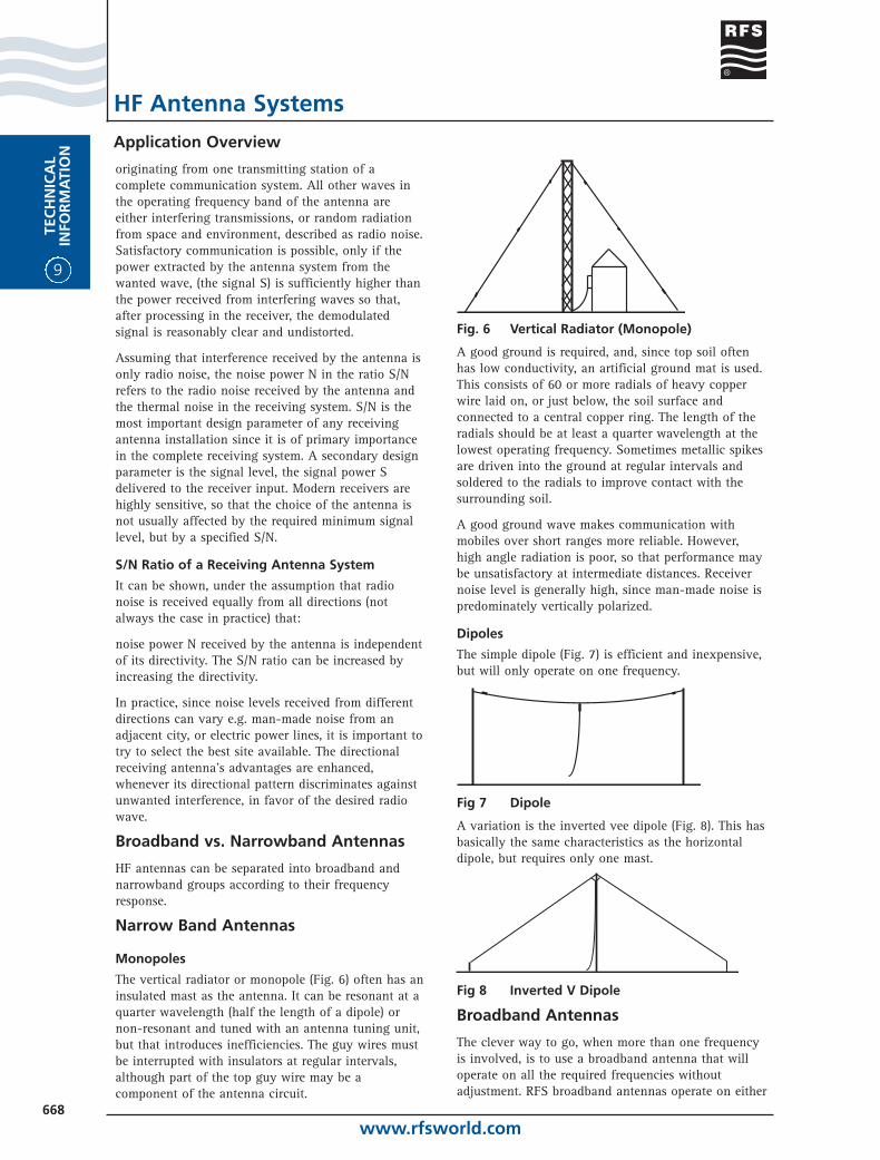
9

TEC

HN

ICA

LIN

FOR

MA

TIO

N

www.rfsworld.com668

Application Overview

HF Antenna Systems

originating from one transmitting station of acomplete communication system. All other waves inthe operating frequency band of the antenna areeither interfering transmissions, or random radiationfrom space and environment, described as radio noise.Satisfactory communication is possible, only if thepower extracted by the antenna system from thewanted wave, (the signal S) is sufficiently higher thanthe power received from interfering waves so that,after processing in the receiver, the demodulatedsignal is reasonably clear and undistorted.

Assuming that interference received by the antenna isonly radio noise, the noise power N in the ratio S/Nrefers to the radio noise received by the antenna andthe thermal noise in the receiving system. S/N is themost important design parameter of any receivingantenna installation since it is of primary importancein the complete receiving system. A secondary designparameter is the signal level, the signal power Sdelivered to the receiver input. Modern receivers arehighly sensitive, so that the choice of the antenna isnot usually affected by the required minimum signallevel, but by a specified S/N.

S/N Ratio of a Receiving Antenna System

It can be shown, under the assumption that radionoise is received equally from all directions (notalways the case in practice) that:

noise power N received by the antenna is independentof its directivity. The S/N ratio can be increased byincreasing the directivity.

In practice, since noise levels received from differentdirections can vary e.g. man-made noise from anadjacent city, or electric power lines, it is important totry to select the best site available. The directionalreceiving antenna’s advantages are enhanced,whenever its directional pattern discriminates againstunwanted interference, in favor of the desired radiowave.

Broadband vs. Narrowband Antennas

HF antennas can be separated into broadband andnarrowband groups according to their frequencyresponse.

Narrow Band Antennas

Monopoles

The vertical radiator or monopole (Fig. 6) often has aninsulated mast as the antenna. It can be resonant at aquarter wavelength (half the length of a dipole) ornon-resonant and tuned with an antenna tuning unit,but that introduces inefficiencies. The guy wires mustbe interrupted with insulators at regular intervals,although part of the top guy wire may be acomponent of the antenna circuit.

Fig. 6 Vertical Radiator (Monopole)

A good ground is required, and, since top soil oftenhas low conductivity, an artificial ground mat is used.This consists of 60 or more radials of heavy copperwire laid on, or just below, the soil surface andconnected to a central copper ring. The length of theradials should be at least a quarter wavelength at thelowest operating frequency. Sometimes metallic spikesare driven into the ground at regular intervals andsoldered to the radials to improve contact with thesurrounding soil.

A good ground wave makes communication withmobiles over short ranges more reliable. However,high angle radiation is poor, so that performance maybe unsatisfactory at intermediate distances. Receivernoise level is generally high, since man-made noise ispredominately vertically polarized.

Dipoles

The simple dipole (Fig. 7) is efficient and inexpensive,but will only operate on one frequency.

Fig 7 Dipole

A variation is the inverted vee dipole (Fig. 8). This hasbasically the same characteristics as the horizontaldipole, but requires only one mast.

Fig 8 Inverted V Dipole

Broadband Antennas

The clever way to go, when more than one frequencyis involved, is to use a broadband antenna that willoperate on all the required frequencies withoutadjustment. RFS broadband antennas operate on either

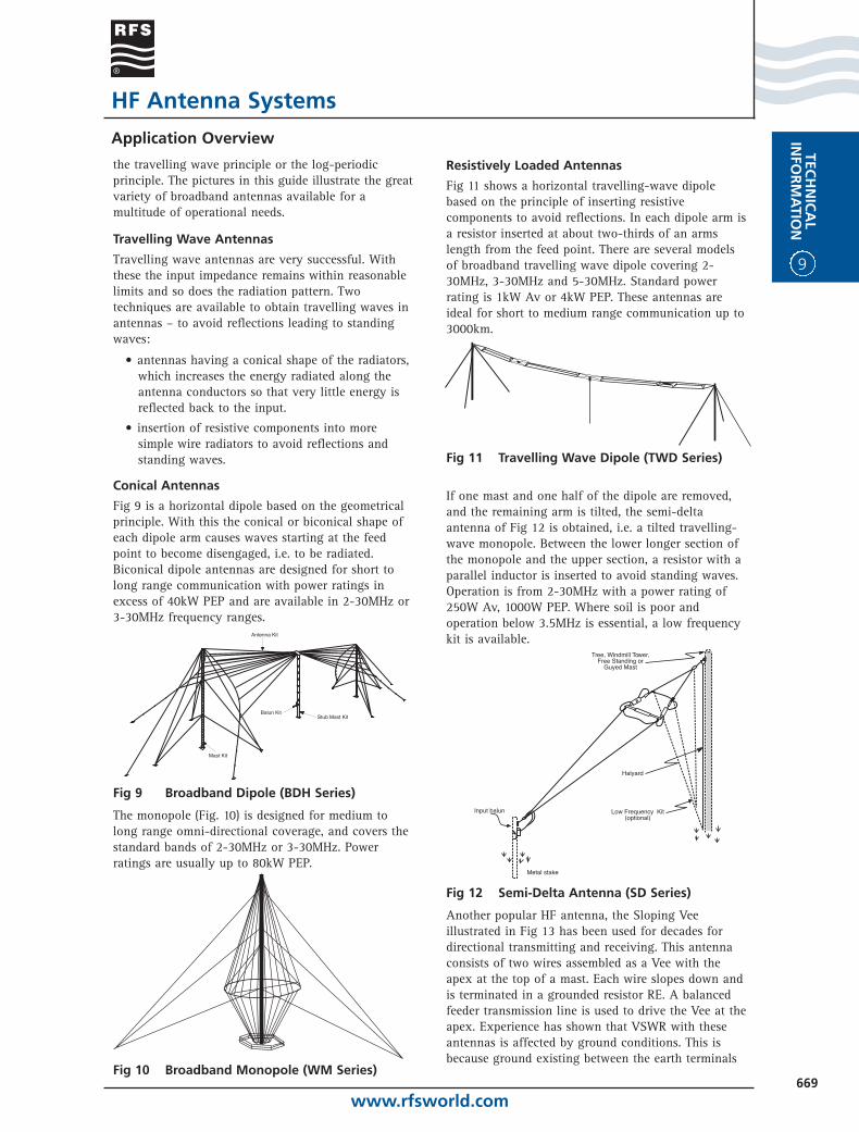
www.rfsworld.com669

TECH

NIC

AL

INFO

RM

ATIO

N

9

Application Overview

HF Antenna Systems

the travelling wave principle or the log-periodicprinciple. The pictures in this guide illustrate the greatvariety of broadband antennas available for amultitude of operational needs.

Travelling Wave Antennas

Travelling wave antennas are very successful. Withthese the input impedance remains within reasonablelimits and so does the radiation pattern. Twotechniques are available to obtain travelling waves inantennas – to avoid reflections leading to standingwaves:

• antennas having a conical shape of the radiators,which increases the energy radiated along theantenna conductors so that very little energy isreflected back to the input.

• insertion of resistive components into moresimple wire radiators to avoid reflections andstanding waves.

Conical Antennas

Fig 9 is a horizontal dipole based on the geometricalprinciple. With this the conical or biconical shape ofeach dipole arm causes waves starting at the feedpoint to become disengaged, i.e. to be radiated.Biconical dipole antennas are designed for short tolong range communication with power ratings inexcess of 40kW PEP and are available in 2-30MHz or3-30MHz frequency ranges.

Fig 9 Broadband Dipole (BDH Series)

The monopole (Fig. 10) is designed for medium tolong range omni-directional coverage, and covers thestandard bands of 2-30MHz or 3-30MHz. Powerratings are usually up to 80kW PEP.

Fig 10 Broadband Monopole (WM Series)

Resistively Loaded Antennas

Fig 11 shows a horizontal travelling-wave dipolebased on the principle of inserting resistivecomponents to avoid reflections. In each dipole arm isa resistor inserted at about two-thirds of an armslength from the feed point. There are several modelsof broadband travelling wave dipole covering 2-30MHz, 3-30MHz and 5-30MHz. Standard powerrating is 1kW Av or 4kW PEP. These antennas areideal for short to medium range communication up to3000km.

Fig 11 Travelling Wave Dipole (TWD Series)

If one mast and one half of the dipole are removed,and the remaining arm is tilted, the semi-deltaantenna of Fig 12 is obtained, i.e. a tilted travelling-wave monopole. Between the lower longer section ofthe monopole and the upper section, a resistor with aparallel inductor is inserted to avoid standing waves.Operation is from 2-30MHz with a power rating of250W Av, 1000W PEP. Where soil is poor andoperation below 3.5MHz is essential, a low frequencykit is available.

Fig 12 Semi-Delta Antenna (SD Series)

Another popular HF antenna, the Sloping Veeillustrated in Fig 13 has been used for decades fordirectional transmitting and receiving. This antennaconsists of two wires assembled as a Vee with theapex at the top of a mast. Each wire slopes down andis terminated in a grounded resistor RE. A balancedfeeder transmission line is used to drive the Vee at theapex. Experience has shown that VSWR with theseantennas is affected by ground conditions. This isbecause ground existing between the earth terminals

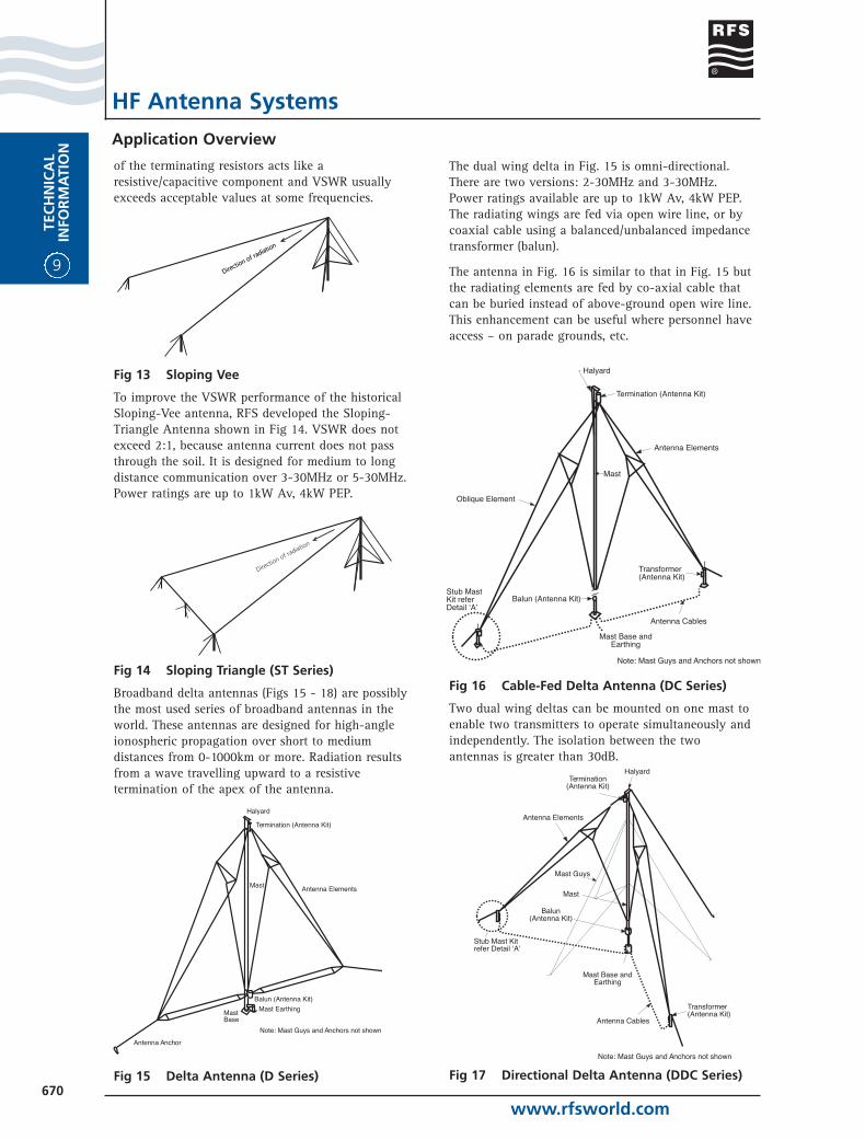
9

TEC

HN

ICA

LIN

FOR

MA

TIO

N

www.rfsworld.com670

Application Overview

HF Antenna Systems

of the terminating resistors acts like aresistive/capacitive component and VSWR usuallyexceeds acceptable values at some frequencies.

Fig 13 Sloping Vee

To improve the VSWR performance of the historicalSloping-Vee antenna, RFS developed the Sloping-Triangle Antenna shown in Fig 14. VSWR does notexceed 2:1, because antenna current does not passthrough the soil. It is designed for medium to longdistance communication over 3-30MHz or 5-30MHz.Power ratings are up to 1kW Av, 4kW PEP.

Fig 14 Sloping Triangle (ST Series)

Broadband delta antennas (Figs 15 - 18) are possiblythe most used series of broadband antennas in theworld. These antennas are designed for high-angleionospheric propagation over short to mediumdistances from 0-1000km or more. Radiation resultsfrom a wave travelling upward to a resistivetermination of the apex of the antenna.

Fig 15 Delta Antenna (D Series)

The dual wing delta in Fig. 15 is omni-directional.There are two versions: 2-30MHz and 3-30MHz.Power ratings available are up to 1kW Av, 4kW PEP.The radiating wings are fed via open wire line, or bycoaxial cable using a balanced/unbalanced impedancetransformer (balun).

The antenna in Fig. 16 is similar to that in Fig. 15 butthe radiating elements are fed by co-axial cable thatcan be buried instead of above-ground open wire line.This enhancement can be useful where personnel haveaccess – on parade grounds, etc.

Fig 16 Cable-Fed Delta Antenna (DC Series)

Two dual wing deltas can be mounted on one mast toenable two transmitters to operate simultaneously andindependently. The isolation between the twoantennas is greater than 30dB.

Fig 17 Directional Delta Antenna (DDC Series)

Direction of ra

diation

Direction of ra

diation

Direction of ra

diation

www.rfsworld.com671

TECH

NIC

AL

INFO

RM

ATIO

N

9

Application Overview

HF Antenna Systems

To enhance the radiation in a particular direction, thetwo arms of a delta antenna can be moved around themast as shown in Fig. 17. This model is known as adirectional delta and extends the range of communi-cation to up to 1600km or more. It is available tocover 2-30MHz and 3-30MHz and power ratings arefrom 1kW Av. to 4kW PEP.

The tandem delta (Fig. 18) is specifically designed forhigh grade short to medium distance circuits forcommunications and HF broadcasting. The tandemdelta does not have a resistive termination at its apex.It is actually two delta antennas. One delta isterminated in another and so nearly 100% of theenergy is radiated, giving the tandem delta a 2dB to4dB gain over the standard delta. Power ratings are upto 80kW PEP.

Fig 18 Tandem Delta Antenna (TDG Series)

Log-periodic Antennas

Wide-band antennas incorporating another principleare log-periodic antennas. These are of particularinterest for high performance HF communicationsystems. They comprise an array of tapered dipoleswith tapered spacing between adjacent dipoles wherethe tapering is constant (i.e. the ratio of adjacentdipole length and adjacent spacing is constant) ineach model. The log-periodic dipole antenna is aresonant antenna. However, due to the tapered config-uration, it is resonant at any operating frequency.Actually only three, four or five dipoles (the so called“active region”), which are close to resonance, operateat the incidental frequency.

Fig 19 Horizontal Log Periodic Dipole Antenna(HLP Series)

The horizontal log periodic dipole array (Fig. 19) is formedium to long distance communication. It isavailable with a wide range of take off angles andgains. Power ratings are from 1 to 20kW Av. andfrequency ranges are from 2-30MHz. No groundscreen is required.

Fig 20 Rotatable Log Periodic Dipole Antenna(HLO Series)

A rotatable version of the horizontally polarized logperiodic antenna is shown in Fig 20. This antenna canbe used to achieve high quality transmission withsome flexibility in selection of the transmissiondirection. The antenna is available in 4-30 MHz and6-30 MHz versions with power ratings up to 10kW Av,40KW PEP.

Fig 21 Vertical Log Periodic Dipole Antenna(VLP Series)

The vertically polarized version shown in Fig 21provides a very low take-off angle for radiation that isideal for long distance communication. Power ratingsare from 1 to 20kW AV, 40kW PEP and frequencyranges are from 3.5-30MHz. For optimumperformance, the low angle radiation can be enhancedby extending a ground screen for several wavelengthsin front of the antenna.

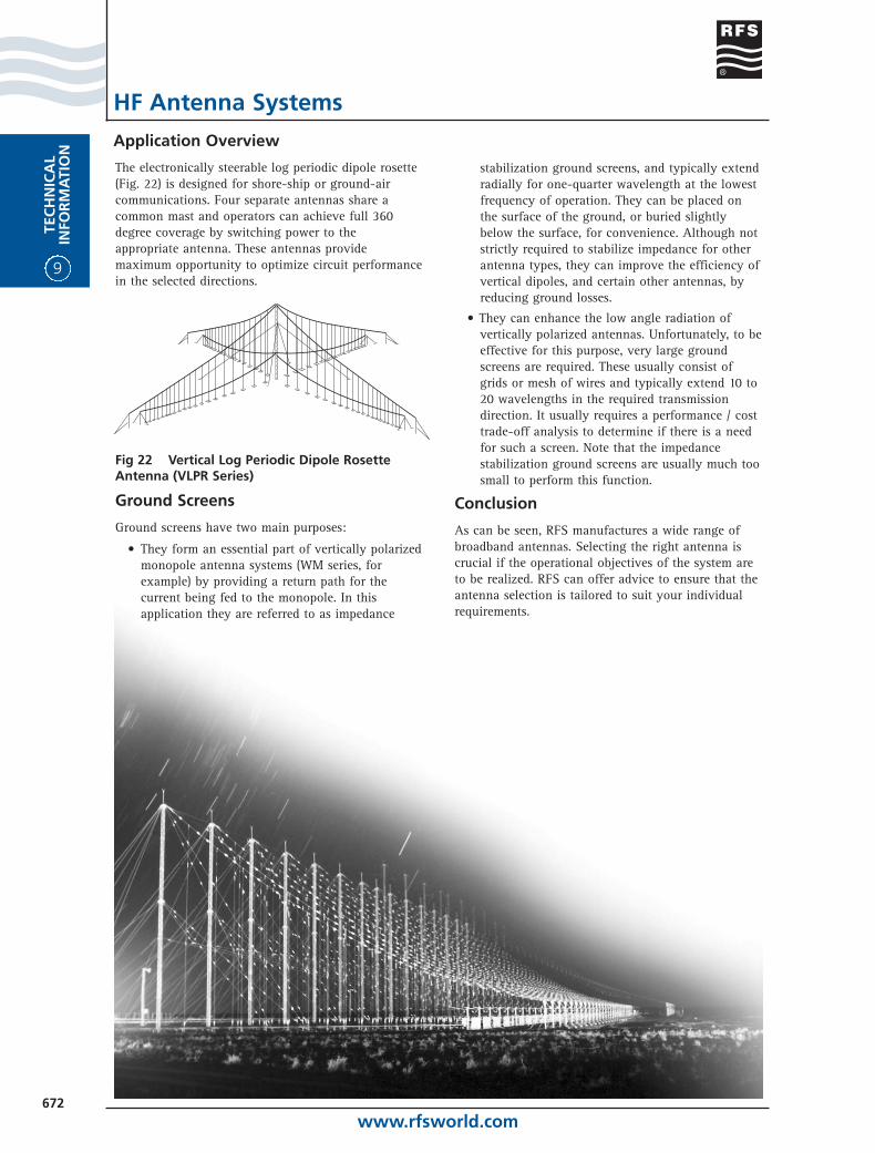
9

TEC

HN

ICA

LIN

FOR

MA

TIO

N

www.rfsworld.com672

Application Overview

HF Antenna Systems

The electronically steerable log periodic dipole rosette(Fig. 22) is designed for shore-ship or ground-aircommunications. Four separate antennas share acommon mast and operators can achieve full 360degree coverage by switching power to theappropriate antenna. These antennas providemaximum opportunity to optimize circuit performancein the selected directions.

Fig 22 Vertical Log Periodic Dipole RosetteAntenna (VLPR Series)

Ground Screens

Ground screens have two main purposes:

• They form an essential part of vertically polarizedmonopole antenna systems (WM series, forexample) by providing a return path for thecurrent being fed to the monopole. In thisapplication they are referred to as impedance

stabilization ground screens, and typically extendradially for one-quarter wavelength at the lowestfrequency of operation. They can be placed onthe surface of the ground, or buried slightlybelow the surface, for convenience. Although notstrictly required to stabilize impedance for otherantenna types, they can improve the efficiency ofvertical dipoles, and certain other antennas, byreducing ground losses.

• They can enhance the low angle radiation ofvertically polarized antennas. Unfortunately, to beeffective for this purpose, very large groundscreens are required. These usually consist ofgrids or mesh of wires and typically extend 10 to20 wavelengths in the required transmissiondirection. It usually requires a performance / costtrade-off analysis to determine if there is a needfor such a screen. Note that the impedancestabilization ground screens are usually much toosmall to perform this function.

Conclusion

As can be seen, RFS manufactures a wide range ofbroadband antennas. Selecting the right antenna iscrucial if the operational objectives of the system areto be realized. RFS can offer advice to ensure that theantenna selection is tailored to suit your individualrequirements.