coded aperture optimization for compressive x-ray ...arce/research_files/angela-23-25-32788.… ·...

Coded aperture optimization forcompressive X-ray tomosynthesis

Angela P. Cuadros,1 Christopher Peitsch,2 Henry Arguello,3

and Gonzalo R. Arce 1,∗1Department of Electrical and Computer Engineering, University of Delaware Newark, DE

19716, USA2Chesapeake Testing Services,Inc. Belcamp, MD 21017, USA

3Department of System Engineering, Universidad Industrial de Santander, Bucaramanga,680002, Colombia∗[email protected]

Abstract: Radiation dose is a concern in X-ray tomographic imaging;coded aperture compressive X-ray tomosynthesis is an approach used toreduce radiation. It places a coded aperture in front of an X-ray sourcein order to obtain 2D patterned projections of a three-dimensional objectonto a detector plane. By using different coded apertures in a multiplesource system, multiplexed projections can be obtained instead of sequen-tial projections as in conventional tomosynthesis systems. Compressedsensing (CS) reconstruction algorithms are then used to recover the three-dimensional data cube. An optimization approach to design the structure ofthe coded apertures in a multiple source compressive X-ray tomosynthesisimaging system is presented. A uniform energy criteria on the voxels anddetector elements is used so that the object is uniformly sensed and theelements of the detector plane uniformly sense the information. Simulationsand experimental results for optimized coded apertures are shown, and theirperformance is compared to the use of random coded apertures.

© 2015 Optical Society of America

OCIS codes: (340.7430) X-ray coded apertures; (340.7440) X-ray imaging; (110.6960) To-mography.

References and links1. J. T. Dobbins III and D. J. Godfrey, “Digital X-ray tomosynthesis: current state of the art and clinical potential,”

Phys. Med. Biol. 48(19), R65 (2003).2. R. Smith-Bindman, J. Lipson, R. Marcus, K.P. Kim, M. Mahesh, R. Gould, A. Berrington de Gonzalez, and D.

L. Miglioretti, “Radiation dose associated with common computed tomography examinations and the associatedlifetime attributable risk of cancer,” Arch. Internal Med. 169(22), 2078–2086 (2009).

3. I. Reiser and S. Glick, Tomosynthesis Imaging (Taylor and Francis, 2014).4. F. Natterer, The Mathematics of Computerized Tomography (Vieweg Teubner Verlag, 1986).5. K. Hamalainen, A. Kallonen, V. Kolehmainen, M. Lassas, K. Niinimaki, and S. Siltanen, “Sparse tomography,”

Computational Methods in Science and Engineering, SIAM, 35, B644–B665 (2013).6. K. Choi and D. J. Brady, “Coded aperture computed tomography,” Proc. SPIE 7468, 74680B (2009).7. Y. Kaganovsky, D. Li, A. Holmgren, H. Jeon, K. MacCabe, D. Politte, J. O’Sullivan, L. Carin, and D. J. Brady,

“Compressed Sampling Strategies for Tomography,” J. Opt. Soc. Am. A 31, 1369–1394 (2014).8. M. Slaney and A. Kak, Principles of Computerized Tomographic Imaging (Society for Industrial and Applied

Mathematics, 2001).9. E. Candes and M. Wakin, “An introduction to compressive sampling,” IEEE Sig. Proc. Mag. 25 (2), 21–30 (2008).

10. A. Cuadros, G. R. Arce, and H. Arguello, “Coded aperture design in compressive X-ray tomography,” in IEEEGlobal Conference on Signal and Information Processing (GlobalSIP), 656–659 Dec (2014).

#252081 Received 16 Oct 2015; revised 5 Dec 2015; accepted 6 Dec 2015; published 11 Dec 2015 © 2015 OSA 14 Dec 2015 | Vol. 23, No. 25 | DOI:10.1364/OE.23.032788 | OPTICS EXPRESS 32788

11. A. Cuadros, K. Wang, C. Peitch, H. Arguello, and G. R. Arce, “Coded aperture design for compressive X-raytomosynthesis,” in Imaging and Applied Optics 2015. Optical Society of America, 2015, p. CW2F.2.

12. J. P. Allebach, “DBS: retrospective and future directions,” Proc. SPIE 4300, 358–376 (2000).13. D. L. Lau and G. R. Arce Modern Digital Halftoning (CRC Press; Taylor & Francis Group, 2008).14. W. Xu, F. Xu, M. Jones, B. Keszthelyi, J. Sedat, D. Agard, and K. Mueller, “High-performance iterative electron

tomography reconstruction with long-object compensation using graphics processing units,” J. Structural Biol.171 (2), 142–153 (2010).

15. D. J. Brady, Optical Imaging and Spectroscopy (Wiley; Optical Society of America, 2009).16. N. Halko, P. G. Martinsson, and J. A. Tropp, “Finding Structure with Randomness: Probabilistic Algorithms for

Constructing Approximate Matrix Decompositions,” SIAM Review, 53(2), 217–288, (2011).17. M. Figueiredo, R. Nowak, and S. Wright, “Gradient projection for sparse reconstruction: Application to com-

pressed sensing and other inverse problems,” IEEE J. Sel. Top. Sig. Proc. 1(4), 586–597 (2007).18. G. R. Arce, D. J. Brady, L. Carin, H. Arguello and D. S. Kittle, “Compressive Coded Aperture Spectral Imaging:

An Introduction,” IEEE Signal Processing Magazine, 105-115, January (2014).

1. Introduction

X-ray tomosynthesis imaging systems have become essential in medical imaging diagnostictasks such as coronary angiography, dual energy imaging and mammography, among others[1]. Recent data suggest that medical radiation exposure may significantly increase the riskof adverse radiation effects, including damage of body cells and even DNA molecules [2].In order to reduce damage that radiation can cause to patients, optimized hardware settingshave been proposed by lowering the number of angles at which projections are taken [3]. Inthis sense, tomosynthesis can be considered a limited-angle computed tomography (CT) thatresults in less radiation exposure for the patient [3]. However, the reduction of measurementsleads to a highly ill-posed inverse problem, sensitive to measurement and modeling errors.Filtered backprojection (FBP) image reconstructions with ill-posed systems of Eqs. produceartifacts and noise that make the reconstructions useless for medical diagnosis [4]. Sparsity-promoting and total variation regularization algorithms have been recently used to improve theill-posed inverse problem, obtaining better image reconstructions [5]. Reducing the number ofangle or projection rays, invariably leads to artifacts in reconstructions. Coded aperture X-raytomography is one approach that can overcome these limitations.

In [6], Choi et al. introduced coded aperture X-ray tomosynthesis, which goes beyond sparseregularization since it allows the acquisition of compressive measurements. The physical cod-ing in coded aperture X-ray tomosynthesis controls the correlation between the measurementvectors. The projections used in [6], however, used random coded apertures. No coded apertureoptimization was considered. The optimization of coded aperture for the coded aperture com-pressive X-ray tomosynthesis system is introduced in the present work, further reducing theradiation exposure in compressive tomosynthesis. Furthermore, multi-frame measurements areobtained by taking sequential snapshots of the object, which leads to more degrees of freedomand improved results. The performance of the optimized codes is compared to that of randomcodes by means of the singular value decomposition (SVD) analysis of the forward operator.

Recently, in [7], Kaganovsky et al. introduced coded aperture projections for medical CTscanner geometries. Random coded apertures are used to modulate the measurements obtainedby varying the angle and detector use for each projection [7]. The methods presented in this pa-per for compressive X-ray tomosynthesis can be extended to the third-generation CT scanners,in which a fan beam X-ray source rotates around the object.

2. Forward projection model

The X-ray transmission imaging model for a single source is given by the Beer-Lambert law[8]: I = I0 · e−

∫ ∞0 μ(x)dx, where I0 is the intensity of a particular X-ray originated from the X-ray

source passing through the object, I is the measured intensity in the detector, and μ(x) is the


Fig. 1. (a) X-ray tomosynthesis. The system matrix Hi determines the mapping of the X-ray cone beam sources to the detector. Each row describes the sensing for a particulardetector element and each column corresponds to the sensing of a particular voxel. (b)Coded aperture compressive X-ray tomosynthesis. The energy of each source is modulatedby means of a coded aperture.

linear attenuation coefficient varying in the location given by x. If such X-ray source is locatedat position �s and illuminates an object in direction θ , the data function for the imaging modelis given by y(�s, θ) = −ln(I/I0). Therefore, Beer-Lambert law can be rewritten as y(�s, θ) =∫ ∞

0 f (�s+ xθ)dx, where f corresponds to the three-dimensional object function, i.e., the X-raylinear attenuation coefficient map. This continuous-to-continuous imaging model is known asthe X-ray transform [3].

The imaging model needs to be discretized since only a discrete number of measurements canbe taken. Thus, the three-dimensional data cube is represented by a vector formed by a discretenumber of unknowns [f] j with j = 0, · · · ,Q− 1 that correspond to the attenuation coefficientsof each of the voxels that constitute the object f ∈R

Q, where Q = Q1 ×Q2 ×Q3 corresponds tothe number of voxels and Q1 is the number of slices of dimensions Q2 ×Q3 each. The detectoris designed to be a two-dimensional plane composed by M = N1 ×N2 detector elements placedunder the object as shown in Fig. 1(a).

The projection measurements are recorded by each of the detector elements such that [y]m ∈R

M for m= 0, · · · ,M−1, corresponds to the mth detector measurement. Tomosynthesis sensingwith a single source i can be written as a finite linear system of Eqs. of the form yi = Hif, wherethe matrix Hi of dimensions M×Q is the system matrix obtained by specifying the hardwaresettings. The weights correspond to the mapping of the cone-beam energy radiating from the X-ray source onto the detector. As shown in Fig. 1(a), each of the elements in the weighting matrixHi, i.e., [Hi]m j, correspond to the portion of the volume of voxel j that is irradiated by the X-rayassociated with the detector element m. Moreover, each of the rows of Hi corresponds to theinformation gathered by one detector and each of the columns corresponds to the informationgathered from a single voxel.

Compressive X-ray tomosynthesis multiplexes measurements from multiple sources onto thedetector. Coded apertures are placed in front of each of the cone-beam sources to modulate theenergy of each X-ray source, producing a particular coded projection onto the detector plane[6]. The coded apertures have the same number of elements as the detector plane. The size of theelements of the coded apertures is fixed to obtain one-to-one correspondence with the detectorelements. The coded aperture Ti is paired to the corresponding ith source, for i = 0, · · · ,P− 1with P being the number of sources with each (u,v) element in the code denoted by (Ti)uv ∈{0,1}, where 0 blocks the X-ray beam and 1 lets the X-ray beam pass. The configuration for thecoded aperture compressive X-ray tomosynthesis is shown in Fig. 1(b). Each of the sources hasa different projection yi and a different system matrix Hi. To account for the coded apertures,the matrix Ci is defined as a diagonal matrix whose diagonal elements are the elements of


the coded aperture Ti, i.e Ci = diag((Ti)00,(Ti)12, · · · ,(Ti)(N−1)(N−1)). Therefore, the sensingprocess for a single source i is given by yi = CiHif.

To generalize the sensing process, C is defined as the matrix concatenating the struc-tures of the coded apertures of the P sources C = [C0|C1| · · · |CP−1], and H is defined asH = [H0|H1| · · · |HP−1]

T . Thus, the measurements for a multiple source system are describedby

y =

(P−1

∑i=0

CiHi

)

f = CHf. (1)

The reconstruction of f from y describes an ill-posed problem; thus, it cannot be solved by theuse of traditional least square approaches. In general, the solution is not unique [4]. However,compressive sensing (CS) asserts that the function f can be recovered, provided two principlesare met: 1) the function f is sufficiently sparse in some basis Ψ, and 2) the basis used to representthe object and the system matrix used to sense the object are incoherent [9].

Let f be represented by f = Ψθ ∈ RQ, where θ is the sparse coefficient representation of

the object, and Ψ is the basis representation. The cumulative sensing at the detector from all Psources is given by y = CHΨθ = AΨθ , where A ∈ R

M×Q is the sensing matrix, with M � Q.The mapping of the energy from all sources onto the detector y captures the modulated energyof all X-ray sources by the coded apertures and the effect of the three-dimensional data-cubeon the coded X-ray field.

The number of compressive measurements obtained by one shot may not be sufficient for ad-equate reconstruction. Therefore, the sensing can be generalized to account for K 2D snapshotprojections and P sources, located in a fixed position. The coded aperture for the ith source andkth shot is denoted by Tk

i , for k = 0, · · · ,K−1. The matrix Cki is the diagonal matrix associated

with Tki . Define Ck = [Ck

0|Ck1| · · · |Ck

P−1], thus yk corresponds to the measurements for the kth

shot, which can be rewritten as yk = CkHΨθ = AkΨθ . Defining y = [y0|y1| · · · |yK−1]T, thesensing process for K shots and P sources is described by:

y = CHf = CHΨθ = AΨθ , (2)

where C = [C0|C1| · · · |CK−1]T. In order to reconstruct the object f, the under-determinedsystem of Eqs. given in (2) is solved by minimizing the cost function ‖y− AΨθ‖2

2 +λ‖θ‖1,where λ is a regularization constant and ‖ · ‖1 and ‖ · ‖2 correspond to the �1 and �2 norms,respectively. This method of data acquisition provides a means to attain multiplexed codedmeasurements.

3. Coded aperture optimization

Multiplexed tomosynthesis introduced by Choi et al. in [6] used random projections generatedby coded apertures with entries randomly distributed. These codes are, in general, sub-optimalsince they do not take into account the fixed geometry of the tomographic system. The codedaperture optimization framework is described next.

3.1. Optimization constraints

Given K tomosynthesis detector measurements, the goal is to design K distinct coded aperturesfor each of the X-ray sources. Let Tk

i be the coded aperture assigned for the ith source and thekth shot. Note that the coded aperture does not depend on the object under inspection but onthe structure of the system matrix H. To achieve incoherent measurements and non-redundantsensing, the coded apertures can be designed such that uniform sensing is achieved under thefollowing criteria.


Criterion 1 Achieve uniform sensing in the detector: Each detector element should measureapproximately the same amount of information, indicating that the detector elements are sens-ing the data cube uniformly. Sensing matrix Ak is binarized so that each entry Ak

mq represents

if the qth voxel is sensed by the mth detector element. Vector dk is defined as the matrix productbetween the matrix Ak and a Q-long one-valued vector μQ = [1, · · · ,1]T i.e. dk = AkμQ, where

dk represents the sum along the M rows of the sensing matrix Ak, i.e. for the kth shot. Sinceeach of the rows of the sensing matrix corresponds to the information related to certain detectorelement, each of the elements of the vector dk represents the number of voxels measured by theaforementioned detector element [10, 11]. For multiple shots, the goal is to reduce the variance

between entries of each vector dk, thus making the entries of the vector d = 1K

K−1∑

k=0dk uniformly

distributed.Criterion 2 Uniformly sense the data-cube voxels: The number of times a certain voxel is

measured should be approximately the same for all voxels. To this end, rk is defined as the ma-trix product between the transpose of the sensing matrix Ak T and an M-long one-valued vectorμM = [1, · · · ,1]T i.e. rk = Ak TμM , where rk represents the sum of the columns of the sensingmatrix for the kth shot. Each of the columns of the sensing matrix is related to a particularvoxel of the three-dimensional object; hence, each of the elements of the vector rk representsthe number of times a particular voxel is measured [10, 11]. For multiple shots, the goal is toreduce the variance between entries of each vector rk, thus making the entries of the vector

r = 1K

K−1∑

k=0rk uniformly distributed.

Criterion 3 Uncorrelated codes for multiple shots: When K ≥ 2, for a particular X-raysource a different set of coded apertures is used in each shot, and Constraint 3 is defined toassure complementary codes are obtained for each source. Specifically, the codes are designedsuch that for a fixed spatial location (u,v) in all the set of coded apertures of a particularsource (Ti)

kuv, only one out of K coded apertures should contain a non-zero value. To this

end, T i is defined as the sum of the K codes for the ith source, i.e. T i =K−1∑

k=0Tk

i . In order to

make the codes uncorrelated, all the entries of T i should be 1. To that end, ST is defined asST = T −UN×PN , where UN×PN corresponds to a one-valued matrix of dimensions N ×PN,T = [T 1| · · · |T P] and c3 as the �0 norm of the vectorized matrix ST , i.e. c3 = ||vect(ST )||0;by minimizing c3 uncorrelated codes are obtained.

Based on the previous three constraints, a cost function that shapes the set of coded aperturessuch that the three-dimensional data cube and the detector plane are sensed as uniformly aspossible while obtaining complementary codes for each source is defined. The cost functionthus aims to minimize the variance of the average number of detector elements measuringeach voxel, i.e., the entries of vector d, the variance of the average number of voxels thateach detector element measures given K shots, i.e., the entries of vector r, and the error termdefined as c3 for the third constraint. Thus, the optimization of the coded apertures for multiplesnapshots is determined by the minimization of the cost function:

argmin[Tk

0,··· ,TkP−1]

k=K−1k=0

α ·M−1

∑m=0

[(d)

m −m1]2+β ·

Q−1

∑j=0

[(r) j −m2

]2+ γ · c3

Subject to(d)

m > 0 and (r) j > 0 ∀ m, j, (3)

where α ≈ 1M since the first term corresponds to the sum of M elements, β ≈ 1

Q since the

second term corresponds to the sum of Q elements, and γ ≈ 1MP since the third term corresponds


Fig. 2. (a) To generate the initial set of codes, vector vkm is defined. It is formed by the values

of the mth elements of the P coded apertures used in the kth shot. (b) Iteration Process forthe DBS algorithm.

to the sum of MP elements. m1 is the desired median of the number of voxels sensed in eachdetector element and m2 is the desired median of the number of times each voxel is sensed. Bothparameters depend on hardware settings. For each of the experiments, the median of the numberof voxels sensed in each detector element and the median of the number of times each voxel issensed are obtained from the vectors d and r obtained when using random codes. Therefore, fordifferent number of shots there are different values for m1 and m2.(d)m corresponds to the mth

element of the average sum of the rows of the sensing matrix for K shots, and (r) j correspondsto the jth element of the average sum of the columns of the sensing matrix for K shots. In orderto solve the optimization problem in (3), the following approach is proposed.

3.2. Optimization algorithm

The Direct Binary Search (DBS) algorithm is an iterative approach to evaluating the effect oftrial changes for each pixel of a binary image for a particular search [12]. Using (3) as a costfunction, optimal coded apertures are obtained using the DBS algorithm to perform a localsearch on each of the coded apertures by either swapping the current pixel with one of itseight nearest neighbors or toggling the coded aperture pixel from 1 to 0 or 0 to 1, keeping thechanges that have positive effects in the cost function and ignoring the changes that have anegative effect. The algorithm stops when, after processing all the K ×P coded apertures, noswaps or toggles occur. Being a steepest descent type of optimization, the DBS algorithm issusceptible to local minimum extrema. Thus the final codes depend on the initial set of codedapertures that are selected [13]. Therefore, an alternative algorithm that takes into account thethree constraints is used to obtain a suitable initial first set of codes.

3.2.1. Initial set of codes

In order to produce an initial set of codes, a binary P long vector vkm =

[(Tk0)m,(Tk

1)m, · · · ,(TkP−1)m] is defined as the concatenation of the values of the mth ele-

ments of the P coded apertures used in the kth shot. The binary vector could take one of 2P −1possible values. The matrix V of dimensions (2P − 1)× P is defined as the concatenationof all possible binary combinations for vector vk

m, such that each of the rows of the matrixcorresponds to one possible value for the vector vk

m as shown in Fig. 2(a). For each location m,K rows of V must be selected; to this end, W is defined as a matrix containing all the possiblecombinations that can be selected from the rows of the matrix V.

To achieve uniform sensing in the detector, while having information only from the mth

pixel, the vector d can be expanded as d = 1K

K−1∑

k=0

[P−1∑

i=0Ck

i Hi

]

μQ = 1K

K−1∑

k=0

P−1∑

i=0Ck

i Gi, where

Gi = HiμQ, i.e., the sum of the rows of the system matrices Hi associated with each source.


Fig. 3. (a) Configuration for X-ray tomosynthesis simulation. 9 sources placed uniformlyover a 128×128 phantom with 16 slices. The dimensions for a general scenario are shownin (a), for the particular simulation scenario that was studied here a = 128,b = 128,c =675,d = 60,e = 150. (b) Mean of the transmittance of the optimal coded apertures for eachshot.

The mth element of the vectors Gi represents the information on how many voxels are measuredin the mth detector when illuminated by the ith source, defining the aforementioned element as(Gi)m and a P-long vector gm = [(G1)m,(G2)m, · · · ,(GP−1)m] the uniformity condition for the

detector plane can be rewritten as: argmin[v0

m,··· ,vkK−1]

k=K−1m=0

[K−1∑

k=0vk T

m gm −m1

]2

.

In order to have complementary codes in the K shots, the following relation has to be met:K−1∑

k=0vk

m = 1, i.e., for the mth location in the K coded apertures of a particular source, only one

of them can have a value of 1.

The algorithm starts selecting all the combinations in W that obeyK−1∑

k=0vk

m = 1 and discards

all the entries of the matrix that do not meet the constraint. From the updated matrix W, thecombinations that achieve uniformity in the detector plane are kept, the other combinations arediscarded. If the matrix W has more than one combination after the two previous iterations, thecombination that minimizes the variance of the mth row of the sensing matrix A is selected, thenthe summation of all the columns of the sensing matrix possess a very low variance, achievinguniform sensing of the object simultaneously.

3.2.2. Efficient DBS algorithm

The DBS algorithm takes an initial set of codes generated with the algorithm described inSection 3.2.1 and the cost function (3) is evaluated and defined as the current error e, i.e. e =

α ·M−1∑

m=0

[[d]

m −m1]2

+ β ·Q−1∑j=0

[[r] j −m2

]2+ γ · c3. Then each pixel from each of the K ×P

codes is visited in a random raster path. For each pixel, the effects of swapping or togglingthat pixel’s value is evaluated in terms of the error e. If one of the nine operations results in areduction of e, such operation is performed and the error term e is updated; otherwise no changein the codes is made. This process is illustrated in Fig. 2(b), where the pixel highlighted in redcan be swapped with its 8 nearest neighbors or toggled to black. The results of each of the nineoperations are shown. In Fig. 2(b), swap operations 1, 2, 4, 5 and 7 would not be consideredsince they do not alter the value of e. Once the operation is completed, the process is repeatedfor the next pixel, which is chosen randomly. The process continues until no change in e is


produced after evaluating all the pixels in all the codes.Updating the error e, implies calculating d, r and c3 for every toggle or swap of a pixel. How-

ever, the multiplication of matrices C and H for the computation of vectors d and r demandssignificant computational resources. To reduce the computational burden of the error calcula-tion, instead of recalculating d and r by the matrix multiplications defined in Section 3.1, analternative definition for the calculation of the constraints is proposed.

Criterion 1 d: using the previous definition developed for the initial codes, d =

1K

K−1∑

k=0

P−1∑

i=0Ck

i Gi and given that Cki is a diagonal matrix, each of the elements of the vector d

can be defined as dm = 1K

K−1∑

k=0

P−1∑

i=0

[Ck

i

]m [Gi]m, where

[Ck

i

]m is the mth element in the main

diagonal of[Ck

i

]. When the mth pixel of a particular Tk

i code is changed or toggled, vector dremains unchanged except for its mth entry in case of a toggle, or m and the entry correspondingto the neighbor of the pixel implied in the swap. Note these changes do not imply the multi-plication of the matrices C and H. Instead, they rely only on the multiplication of the entriesinvolved in the change, i.e.,

[Ck

i

]m and [Gi]m.

Criterion 2 r: this constraint is related to the sum of the columns of matrix Hi. Therefore, aswap or a toggle of one of the elements of the codes results in changing all the elements of thevector r as opposed to the previous constraint. To obtain a simplification of the original expres-

sion for constraint 2, it is expanded as: r = 1K

K−1∑

k=0

P−1∑

i=0

[Ck

i Hi]T μM = 1

K

K−1∑

k=0

P−1∑

i=0HT

i Ck Ti μM =

1K

K−1∑

k=0

P−1∑

i=0HT

i Jki , where Jk

i = Cki μM is a column vector composed by the components of code

Tki . From the previous expression it can be seen that the mth element of the code multiplies all

the elements of the mth column of the matrix HTi , i.e., all the elements of the mth row of matrix

Hi. Since the elements of the coded apertures are binary 0,1, a toggle of the mth pixel will resultin the subtraction (change of the pixel from 1 to 0) or addition (change of the pixel from 0 to 1)of the elements of the mth row of the matrix Hi to the current vector r.

The efficient DBS optimal process is summarized as follows:

1. Generate the initial set of codes, and calculate the initial error e.

2. For each pixel in the coded apertures, evaluate the effect of all possible trial changesusing the modified constraints and the definition for c3. Perform the change that resultsin a lower e.

3. Stop when, after processing all the K×P coded apertures, no swaps or toggles occur.

4. Simulations

To simulate the compressive X-ray tomosynthesis configuration, a scenario with a flat 2D de-tector plane composed by N1 ×N2 = 150 × 150 elements, P = 9 cone-beam X-ray sourcesplaced uniformly in a 3×3 geometry and an object of interest f represented by a Q2×Q3×Q1 =128× 128× 16 are used, each of the pixels in the coded aperture corresponds to a particulardetector element as detailed in Fig. 3(a). Therefore, the coded apertures placed in front of eachof the sources are also composed by 150× 150 elements. The ASTRA Tomography Toolbox(“All Scale Tomographic Reconstruction Antwerp”) [14] was used to obtain the system matri-ces Hi as well as the projection measurements yi of each of the X-ray cone beam sources. Usingthe algorithm described in Section III, optimal coded apertures for K = 1 and K = 2 shots areobtained. The performance of random coded apertures and the optimal codes is compared usingthe singular value analysis.


Fig. 4. (a) Singular Value Decomposition of the tomosynthesis matrix without coding, op-timized codes and random codes for K=1 and K=2 shots (b) Singular Value Decompositionfor the last 6900 components.

4.1. Singular value analysis

When two different measurement strategies are used to sense an object, the singular value de-composition (SVD) analysis can provide a simple mechanism for comparison [15]. The SVD ofthe matrix A for the compressive X-ray tomosynthesis system showed in Fig. 4(a) is calculated.Scenarios of K = 1 and K = 2 shots are considered. For the latter case, a randomized methodfor computing an approximate singular value decomposition [16] is used due to the size of thematrix A. Therefore, only the first 22500 nonzero singular values of the matrix A are obtained.Three different cases are analyzed for K=1 and K=2: (A) No coding (A = H), which is equiva-lent to setting all the pixel elements of all the coded apertures to 1, for K = 2 the singular valuedecomposition is equivalent to K = 1 for this particular case; (B) Optimized codes using thealgorithm previously described and the parameters describing the hardware settings A = CHare obtained and; (C) The coded aperture elements are generated randomly. For the latter, themean for 20 different selections is obtained. Figure 4(a) presents the singular value decompo-sition for the cases previously discussed. Considering there is no prior information abut theobject under inspection, the measurement strategy that has more singular value componentslying above certain noise level is considered to outperform the others, since it would capturemore orthogonal components of the object. Thus, note that both random coding and optimizedcodes outperform, for any noise level, the case when no coding is used for both K = 1 andK = 2 shots. Additionally, the singular value spread for the curves corresponding to K = 1 islarger than for K = 2 thus showing that an increase in the number of shots results in a bettermeasurement strategy to sense the object.

Two different noise levels are used in Fig. 4(a). It can be seen that for the higher noise levelin the case of a single shot both optimized codes and random codes have similar behavior.However, for lower noise levels the optimized codes show better performance than the randomcodes, as it is shown in Fig. 4(b). For K = 2, Fig. 4(a) shows that optimized codes outperformrandom codes for both noise levels. From the SVD analysis, it can be concluded that optimizedcodes can provide advantage over random codes even under noisy conditions. This will bedemonstrated in Section V for real data results.

For K = 1 and K = 2, the problem is very ill-conditioned. It can be noted that the number ofmeasurements is much lower than the number of unknowns (voxels). The condition number (ra-tio of greatest singular value to the least nonzero singular value κ) measures how ill-conditionedthe problem is [15]. The condition number (κ) for the three cases studied in this section forK = 1 show that when using optimized codes the sensing matrix becomes less ill-conditioned


Fig. 5. Histogram of the number of voxels measured by a detector element, d. (a) Beforethe optimization, (b) After the optimization.

Fig. 6. (a) Histogram of the number of detectors that measure a certain voxel, r. (a) Beforethe optimization, (b) After the optimization.

(κ = 15.60) compared to using random codes (κ = 562.12) or no coding (κ = 20.49), showingthat uniformly sensing of the detector plane and the data cube leads to better conditioning ofthe forward operator.

4.2. Results

Experimental tomography data was obtained at Chesapeake Testing Inc., with a Nikon metrol-ogy 225/450kV Vault CT scanning system with a 450kV micro-focus X-ray source capable ofproducing a spot-size down to 80um. The detector is a 16in×16in square plane and the detectorpitch is 200um. Multiple X-ray projections over 360 degrees around an object, in this particularcase a vivofit watch, are acquired. These projection images are then reconstructed into a full 3Dvolumetric data set.

This 3D data cube is re-sampled to obtain the data cube of size 128× 128× 16 describedat the beginning of Section IV. Assuming that the line integrals are measured directly and thehardware settings previously described, the measurements y and the matrix H are obtained asdescribed in (1). The set of coded apertures Tk

i with i = 0, · · · ,P−1 and k = 0, · · · ,K −1 wasacquired using the algorithm for the coded aperture design introduced in Section III. It can beseen in Fig. 3(b) that the transmittance (τλ ) decreases as the number of shots increase given


Fig. 7. (a) Thirteenth slice of the data cube. Sparse regularized reconstructions from: (b)Random coded X-ray projections using 3 snapshots (PSNR=25.96 dB); (c) Optimizedcoded apertures using 3 snapshots (PSNR=29.68 dB); (d) Uncoded X-ray projections using1 snapshot (PSNR= 23.60 dB). Zoomed versions of: (e) Random coded X-ray projections;(f) Optimized coded apertures.

the constraint that the codes have to be complementary. The reconstruction algorithm used torecover the data cube is the GPSR (Gradient Projection for Sparse Reconstruction) [17]. Thesignal representation basis used to represent the three-dimensional data cube is a Kroneckerproduct of a 2D wavelet transform and a 1D discrete Fourier transform (DCT) [18] . For K = 3,Figs. 5 and 6 show the histograms corresponding to the number of voxels measured by onedetector and the number of detectors that measure certain voxel respectively. Figure 5(a) showsthe distribution of the entries of the vector d before the optimization. Figure 5(b) shows that thedistribution of the entries of vector d become concentrated around m1 = 32.47; thus an averageof 32 voxels are measured per detector, after the optimization. The initial distribution of theentries of the vector r is shown in Fig. 6(a). After the optimization, a more uniform distributionconcentrated around m2 = 3.21 is obtained, as shown in Fig. 6(b); thus, every voxel is sensedan average of 3 times. The peak signal-to-noise ratio (PSNR) is used to compare the reconstruc-tions obtained since it is suitable for comparing restoration results as it does not depend stronglyon the image intensity scaling. For a scenario with an image I and a reconstruction R of size

N ×N it is defined as PSNR = 10 log10

(Max2

IMSE

), where MaxI is the maximum possible pixel

value of the image I and MSE = 1N2 ∑N−1

i=0 ∑N−1j=0 [I(i, j)−R(i, j)]2. Table 1 shows the PSNR of

the reconstructions of the thirteenth slice for K = 1,2,3,4 and 5 and for optimized codes andrandom codes. The elements of the random coded apertures used are random realizations ofBernoulli random variables, with different levels of transmittance. For the multi-frame scheme,the transmittance of the codes is fixed depending on K for one case and for comparison, anotherscenario is analyzed when the transmittance is fixed to τλ = 0.5. The compression ratio, will begiven in each case by ρ = 1− (M×K)/Q. Therefore, maximum compression is obtained whena single shot is used. It can be seen that as the number of shots increases the reconstructionquality improves. Nonetheless, the improvement is not significant after 3 shots, for the scenarioused for the simulations, since the number of unknowns is limited. For a data cube composedby more slices, increasing the number of shots would lead to further improvement. Clearly, thebest results are obtained using the optimized coded apertures (first column in Table 1).


Table 1. PSNR of the reconstructed image of the 13th slice for different number of shots(K)

ShotsPSNR (dB) ρ

Optimal Codes τ∗λ = 0.5 τλ = 1/K1 26.36 24.83 24.67 91.41%2 28.29 25.82 25.92 82.83%3 29.68 25.96 26.14 74.25%4 29.76 26.45 26.48 65.67%5 29.89 27.17 27.57 57.08%

Figure 7(a) shows the thirteenth slice of the three-dimensional data cube used for the simula-tions. By acquiring uncoded measurements from 1 snapshot (A = H), the reconstruction shownin Fig. 7(d) is obtained. Coded X-ray projections are next used in the measurements where ran-dom binary patterns with transmittance τλ = 0.5 are used as coded apertures. For this scenario,3 snapshots are used. The measurement set is now less correlated, such that improved recon-structions are obtained as depicted in Fig. 7(b). As stated in previous sections, random codesdo not exploit the known geometry of the tomographic system. By applying the optimizationalgorithm described in Section 3, with m1 = 32.47 and m2 = 3.21, the improvement in the re-construction PSNR can be observed in Fig. 7(c). Moreover, Figs 7(e) and 7(f) show zoomedversions of the reconstructions obtained when using random codes and optimized coded aper-tures respectively. The PSNR gain is evident in the zoomed versions of the reconstructions.The PSNR for slice 13 for random codes and K = 3 shots is 25.96 dB, for optimized codes is29.68 dB and for the least squares approach is 29.10 dB. For the latter, least squares estimationis used to reconstruct the X-ray tomosynthesis problem, i.e. when each source produces a setof measurements on the detector. Note that the traditional least squares reconstruction uses 3times the amount of measurements than the compressive X-ray tomosynthesis approach withK = 3 shots. Furthermore, the latter reduces the radiation exposure of the patient/sample.

For the simulation results slice 1 is the closest slice to the sources and slice 16 is the slicelocated farthest away from the sources. Table 2 shows the PSNR of the reconstruction of the16 slices of the data cube for K = 3 shots, for both optimized codes and random codes. Fur-thermore, Figs. 8(a) and 8(d) depict the slices 1 and 16 of the original data cube respectively,and the reconstructions obtained when using optimized coded apertures and K = 3 snapshotsare shown in Figs. 8(b) and 8(e) for each of the slices. Figures 8(c) and 8(f) depict the leastsquares reconstructions for slices 1 and 16 respectively, where least squares estimation is usedto reconstruct the X-ray tomosynthesis problem when the full set of X-ray projections are used.

Table 2. PSNR of the reconstructed image of the 16 slices of the data-cube for K = 3 shots

Slice 1 2 3 4 5 6 7 8Optimized (PSNR dB) 28.5 27.6 29.2 27.8 27.7 27.3 27.7 26.8

Random (PSNR dB) 24.7 25.5 25.7 25.7 26.3 26.4 26.1 26.1Slice 9 10 11 12 13 14 15 16

Optimized (PSNR dB) 26.4 27 28 29.3 29.7 29.7 29.6 25.4Random (PSNR dB) 25.9 26.3 26.5 24.9 26 24.5 24.1 22.6

The optimized coded apertures used for the central source and the source located in thelower right corner for K = 2 are depicted in Fig. 9. Figures 9(a) and 9(b) depict the coded


Fig. 8. (a) First slice of the data cube. (b) Sparse regularized reconstructions from optimizedcoded apertures using 3 snapshots (PSNR=28.47 dB). (c) Least squares reconstruction us-ing the full matrix (PSNR=28.27 dB); (d) 16th slice of the data cube. (e) Sparse regularizedreconstructions from optimized coded apertures using 3 snapshots (PSNR=25.45 dB). (f)Least squares reconstruction using the full matrix (PSNR=25.46 dB). Note that LS recon-structions uses 3 times the amount of measurements than the compressive X-ray tomosyn-thesis.

Fig. 9. Optimal coded apertures for: Two snapshots (K=2), (a) the central source and firstsnapshot, (b) the central source and second snapshot, (c) the source located in the lowerright corner and first snapshot, (d) the source located in the lower right corner and secondsnapshot.

apertures corresponding to the source located in the center and for K=2, Figs. 9(c) and 9(d)correspond to the coded apertures used for the source located in the lower right corner forK=2. Notice the non-uniform density of the designed codes as well as the structured patterns,which also vary from location to location. Optimized coded apertures for K = 3 and the centralsource are depicted in Fig. 10; the decrease in the transmittance (τλ ) is evident between thecoded apertures used for K = 2 (Fig. 9) and K = 3 (Fig. 10). A one-dimensional cross-sectionof coded aperture elements in column 50, rows 130 to 140 in each of the codes used for thecentral source is shown in Fig. 10. Note for 9 of the 10 cases analyzed, only one out of 3 codedapertures contains a non-zero value for a specific spatial location in the codes, which was thecondition to assure complimentary codes.

Convergence of the DBS algorithm as stated in Section 3.2 depends on the initial set of codedapertures that are selected, Fig. 11(a) presents the convergence of the DBS algorithm whenusing random codes and a set of checkerboard codes as opposed to the optimized initialization


Fig. 10. Optimal coded apertures for three snapshots (K=3) and the central source and a 1Dcross section of the coded aperture elements in column 50, rows from 130 to 140.

Fig. 11. (a) Convergence of DBS algorithm for different initial set of codes: (blue) checkerboard, (red) optimized set of codes, (black) random set of codes. (b) Convergence of DBSalgorithm for the first 1.42 days (122,500 seconds)

proposed, for the simulation scenario previously discussed. Note that using a predefined pattern(checkerboard) results in a higher error compared to both initial random and optimized codedapertures. Furthermore, the initial error, the time of convergence and the final error are higherfor random coded apertures compared to the initial optimized set of coded apertures as depictedin Fig. 11(b).

5. Testbed implementation

Experimental tomosynthesis data was obtained at Chesapeake Testing Inc. with the systemdescribed in Section IV. The energy used for the source is 245keV and five projections cor-responding to five different locations of the same source were obtained. The source is movedalong one line due to constraints of the testbed system. To obtain the measurements, the sourceis moved 4 times, 5cm at a time from the center position, which is aligned with the center of thedetector. The detector remains static for all the measurements. The sources were located 892mmaway from the object and the detector was placed 1100mm away from the source. The objectimaged is a RJ45 cable, discretized as 12 slices of 128×128 pixels with voxels of dimensions0.4mm×0.4mm×0.8mm. The detector was composed of 140×240 elements and the size of thedetector elements was 0.4mm. Figures 12(a)(b) depict the projections obtained from the central


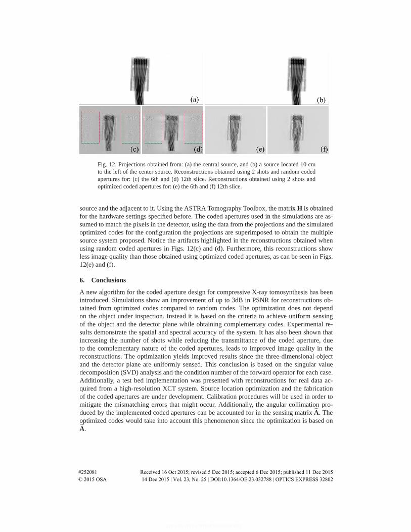
Fig. 12. Projections obtained from: (a) the central source, and (b) a source located 10 cmto the left of the center source. Reconstructions obtained using 2 shots and random codedapertures for: (c) the 6th and (d) 12th slice. Reconstructions obtained using 2 shots andoptimized coded apertures for: (e) the 6th and (f) 12th slice.

source and the adjacent to it. Using the ASTRA Tomography Toolbox, the matrix H is obtainedfor the hardware settings specified before. The coded apertures used in the simulations are as-sumed to match the pixels in the detector, using the data from the projections and the simulatedoptimized codes for the configuration the projections are superimposed to obtain the multiplesource system proposed. Notice the artifacts highlighted in the reconstructions obtained whenusing random coded apertures in Figs. 12(c) and (d). Furthermore, this reconstructions showless image quality than those obtained using optimized coded apertures, as can be seen in Figs.12(e) and (f).

6. Conclusions

A new algorithm for the coded aperture design for compressive X-ray tomosynthesis has beenintroduced. Simulations show an improvement of up to 3dB in PSNR for reconstructions ob-tained from optimized codes compared to random codes. The optimization does not dependon the object under inspection. Instead it is based on the criteria to achieve uniform sensingof the object and the detector plane while obtaining complementary codes. Experimental re-sults demonstrate the spatial and spectral accuracy of the system. It has also been shown thatincreasing the number of shots while reducing the transmittance of the coded aperture, dueto the complementary nature of the coded apertures, leads to improved image quality in thereconstructions. The optimization yields improved results since the three-dimensional objectand the detector plane are uniformly sensed. This conclusion is based on the singular valuedecomposition (SVD) analysis and the condition number of the forward operator for each case.Additionally, a test bed implementation was presented with reconstructions for real data ac-quired from a high-resolution XCT system. Source location optimization and the fabricationof the coded apertures are under development. Calibration procedures will be used in order tomitigate the mismatching errors that might occur. Additionally, the angular collimation pro-duced by the implemented coded apertures can be accounted for in the sensing matrix A. Theoptimized codes would take into account this phenomenon since the optimization is based onA.


coded aperture optimization for compressive x-ray ...arce/research_files/angela-23-25-32788.… ·...

Documents