coequational logic for finitary functors

Coequational Logic for Finitary Functors

Daniel Schwencke 1,2

Department of Theoretical Computer ScienceInstitute of Technology,Braunschweig, Germany

Abstract

Coequations, which are subsets of a cofree coalgebra, can be viewed as properties of systems. In caseof a polynomial functor, a logic of coequations was formulated by J. Adamek. However, the logic is morecomplicated for other functors than polynomial ones, and simple deduction rules can no longer be formulated.A simpler coequational logic for finitely branching labelled transition systems was later presented by theauthor. The current paper carries that research further: it yields a simple coequational logic for finitaryfunctors that preserve preimages. Furthermore we prove a statement for semantical consequences of sets ofcoequations in the case of accessible functors.

Keywords: cofree coalgebra, coequation, logic, finitary functor, preimage

1 Introduction

Several authors studied logics that formalise properties of systems described ascoalgebras over a set functor. On the one hand, modal logics were investigatede. g. by Lawrence Moss [8] or Dirk Pattinson [9]. On the other hand, dualizingequational presentations of algebras, Jan Rutten [10] introduced coequations assubsets of cofree coalgebras. These coequations can also be used to establish logicsof system properties, see e. g. the work of Jesse Hughes [7]. Our paper deals witha coequational logical topic different to the one of Hughes. In [1] Jiri Adamekformulated a logic of coequations and proved it to be sound and complete. Sincethe elements of a cofree coalgebra for a fixed functor can be viewed as “behaviourpatterns” of coalgebras for this functor, coequations describe certain properties ofsuch coalgebras. Thus with a logic of coequations we are able to obtain propertiesof a coalgebra automatically from other properties of this coalgebra.

Coequational logic provides a deduction system to derive coequations from agiven set of assumed coequations. It is particularly simple in case of polynomial

1 The grant of DFG is gratefully acknowledged.2 Email: [email protected]

Electronic Notes in Theoretical Computer Science 203 (2008) 243–262

1571-0661/$ – see front matter © 2008 Elsevier B.V. All rights reserved.

www.elsevier.com/locate/entcs

doi:10.1016/j.entcs.2008.05.028

mailto:[email protected]

http://www.elsevier.com/locate/entcs

functors: the cofree coalgebra consists of coloured trees, and the deduction systemhas only two rules, the subtree rule and the recolouring rule. The logic for accessiblefunctors is more complicated.

In this paper we focus on finitary functors, a subclass of accessible functors.Our prime example is the finite power-set functor Pf (A × −): the correspondingsystems are the finitely branching labelled transition systems (LTS), and our paperis a generalisation of the logic for LTS presented in the thesis [11]. That logicfor LTS is based on the presentation of the cofree Pf (A × −)-coalgebra as theset of all “strongly extensional” trees, which were indroduced by James Worrellin [12]. Coming back to an abstract finitary functor H, we show how to obtaina presentation of its cofree coalgebra as a set of trees. Using that presentation,under the relatively weak assumption that H preserves preimages we formulate acoequational logic which is nearly as simple as the one for polynomial functors andprove it to be sound and complete. This way we provide a simple coequational logicfor a wide range of relevant non-polynomial functors.

A little section at the end shows a result about semantical consequences ofarbitrary subsets of cofree coalgebras of accessible functors, whereas coequationsare special subsets of cofree coalgebras.

2 Coequational logic

2.1 Preliminaries

Since we are working with coalgebras (sometimes also referred to as “systems”) asstructured sets all functors considered will be endofunctors of Set in the categorySet of sets and functions. We already mentioned some special cases in the previoussection:

• A polynomial functor for a given signature Σ is a functor of the shape

∑

σ∈Σ

(−)nσ ,

where nσ is the arity of the operation σ ∈ Σ. The signature is called k-ary ifnσ < k for all σ ∈ Σ, where k is some infinite regular cardinal.

• A finitary functor H is a functor preserving filtered colimits, or equivalently, itis a quotient of some polynomial functor HΣ for a finitary signature Σ. Thismeans there exists a natural transformation ε : HΣ → H having surjective com-ponents, where the arities nσ of all operations σ ∈ Σ are finite. For equivalentcharacterisations of finitary functors see [5].

• An accessible functor is a functor preserving k-filtered colimits for some infiniteregular cardinal k, or equivalently, it is quotient of some polynomial functor HΣ

for a k-ary signature Σ. Each finitary functor is accessible (k = ω). For equivalentcharacterisations of accessible functors see [4].

D. Schwencke / Electronic Notes in Theoretical Computer Science 203 (2008) 243–262244

For a polynomial functor HΣ we shall denote the terminal coalgebra and thecofree coalgebra on some fixed countable infinite set C of colours by TΣ and QΣ

respectively. Their structure maps are denoted by αTΣ: TΣ → HΣTΣ and αQΣ

:QΣ → HΣQΣ, the couniversal colouring arrow of QΣ by γΣ : QΣ → C. Analogously,for a finitary functor H we shall write T and Q, αT , αQ and γ.

All trees considered in the paper are rooted, ordered trees that arise from asignature Σ, i. e. every node is labelled with an operation symbol σ ∈ Σ and hasexactly nσ children, where nσ is the arity of σ. These trees are called Σ-trees. Wealways consider trees up to isomorphism, e. g. if we the take the set of all subtreesof a tree it is meant to contain no duplicates rooted at different positions.

For a polynomial functor HΣ it is well-known that TΣ consists of all Σ-trees andthat αTΣ

sends a Σ-tree to its root label (the operation symbol) and the list of itssubtrees, see e. g. [4]. Similar, the cofree HΣ-coalgebra QΣ consists of all colouredΣ-trees; that is, every node carries two labels: an operation symbol from Σ and acolour from C. The map αQΣ

sends a coloured Σ-tree to its root operation symboland the list of its coloured subtrees; γΣ maps every coloured Σ-tree to its rootcolour.

For a finitary signature Σ (i. e. the Σ-trees from TΣ are finitely branching) itholds that if Σ is linearly ordered, so is TΣ in the following sense: we compare twotrees from TΣ by breadth-first search. Starting at the roots (depth n = 0), as longas we find only equal operation symbols at the nodes of depth n, it is always assuredthat we can compare the nodes of depth n+1 from left to right. As soon as we findtwo nodes with different operation symbols, the order of the trees is given by theorder of these operations. It is easy to verify that this way we obtain a linear orderof all trees from TΣ: the transitivity is easy to see and the completeness follows fromthe facts that two different trees (even those of infinite depth) have to differ withinfinite depth and that these trees are finitely branching, thus every finite depth canbe reached by breadth-first search. Therefore, if Σ×C is linearly ordered, so is QΣ

in the same sense.

2.2 Coequations

Definition 2.1 Given a cofree coalgebra Q, a coequation is a coatomic subset Q \{q} for some q ∈ Q. Since it is completely described by the element q, we shalldenote it by �q (read: avoid q).

These coatomic sets are called coequations because they are the coalgebraicdual to equations in universal algebra: while the latter determine quotients of freealgebras, the former determine quotients of cofree coalgebras.

Definition 2.2 Let (Q, αQ, γ) be the cofree H-coalgebra on C. An H-coalgebra(S, αS) is said to satisfy a coequation �q if for all colourings f : S → C and forall states s ∈ S we have f∗(s) �= q for the unique homomorphism f∗ : S → Q withf = γ ◦ f∗. More generally, (S, αS) is said to satisfy a subset U ⊆ Q of the cofreecoalgebra if for all colourings f : S → C we have f∗[S] ⊆ U .

D. Schwencke / Electronic Notes in Theoretical Computer Science 203 (2008) 243–262 245

Remark 2.3 The coequations introduced by Jan Rutten are defined more generallyas subsets U ⊆ Q. As we see from the above Definition 2.2, for every coalgebra tosatisfy a subset U ⊆ Q is equivalent to satisfying all coequations �q where q ∈ Q\U ,i. e. U can be expressed via coequations by U =

⋂q∈Q\U �q. This means that when

investigating subsets of cofree coalgebras, we can restrict ourselves to coequations,a fact that was first observed by Peter Gumm [6].

Since the elements of the cofree H-coalgebra can be viewed as “behaviour pat-terns” of H-coalgebras and the pattern q is forbidden by the corresponding coequa-tion �q, coequations can be regarded as certain “system properties”. Coequationsstand for exactly these system properties preserved by coproducts, homomorphicimages and subsystems. This follows from the Co-Birkhoff Theorem proven by JanRutten [10].

Definition 2.4 A coequation �q is said to be a semantical consequence of a co-equation �q′ if every H-coalgebra that satisfies �q′ also satisfies �q. We shalldenote this by �q′ |= �q. More generally, a subset U ⊆ Q is said to be a semanticalconsequence of a subset U ′ ⊆ Q if every H-coalgebra that satisfies U ′ also satisfiesU , notation U ′ |= U .

2.3 A logic of coequations

When presenting a logic of coequations, we first define what proofs in that logic willbe and then state some soundness and completeness results.

Definition 2.5 Let P be a set of coequations (the premise). A proof in a coequa-tional logic of a coequation �q is a list of coequations �ci, i ≤ l of lenght l + 1,where l is some ordinal, where �cl = �q and where for every i ≤ l it holds that�ci ∈ P or F |= �ci, where F ⊆ {�cj |j < i}.

Let us consider systems of polynomial functors HΣ. We call two nodes v, w ofa tree t ∈ QΣ equivalent, if the coloured subtrees tv and tw of t rooted at v and w,respectively, are isomorphic.

Definition 2.6 Given a cofree coalgebra QΣ of a polynomial functor, a recolouringof a tree t ∈ QΣ is a tree r ∈ QΣ for which there exists a homomorphism h : QΣ →QΣ such that h(t) = r.

Remark 2.7 As shown in [1], this is equivalent to the following: t and r have thesame shape and for any two equivalent nodes in t the corresponding nodes in r areequivalent again.

Example 2.8 Let HΣ = (−)2 + 1, i. e. Σ contains a binary operation σ and aconstant c. Then QΣ consists of all coloured binary trees. Consider the followingtwo trees from QΣ:


σ

c σ

c c

σ

c σ

c c

The right-hand tree is a recolouring of the left-hand one: both trees have thesame shape and the black leaves of the left-hand one (which are the only equivalentnodes in this tree) are equivalent in the right-hand one. Note that the converse isnot true since in the right-hand tree all leaves are equivalent nodes but this is notso in the left-hand one.

Before we restate the main result for coequational logic of polynomial functors,we introduce a relation on QΣ as follows: for two trees t, r ∈ QΣ we write r � t, ifr is a recolouring of a subtree of t.

Theorem 2.9 ([1]) For a polynomial functor HΣ a coequation �t is semanticalconsequence of the coequations �ri, i ∈ I, if and only if there is some ri that is arecolouring of some subtree of t, shortly

⋂

i∈I

�ri |= �t ⇐⇒ ∃i ∈ I : ri � t.

Corollary 2.10 ([1]) For systems of a polynomial functor deduction of coequationswith the following rules is sound and complete:

(i) child rule�tv�t

where v is a child of the root of t

(ii) recolouring rule�r

�twhere r is a recolouring of t

Now we can go one step further and consider systems as coalgebras of an ac-cessible functor H. These are quotients of polynomial functors HΣ, i. e. there is anatural transformation ε : HΣ → H with surjective components. From this one canderive that the cofree H-coalgebra Q on C is quotient of the cofree HΣ-coalgebraQΣ on C, see [1]. Thus Q consists of equivalence classes of coloured Σ-trees, whichwe call ε-classes. Given a cofree H-coalgebra Q, we denote by [t] ∈ Q the ε-class ofa Σ-tree t ∈ QΣ from the corresponding cofree HΣ-coalgebra QΣ.

Theorem 2.11 ([1]) For an accessible functor H a coequation �q is a semanticalconsequence of the coequations �qi, i ∈ I, if and only if for every tree t ∈ QΣ with[t] = q there is some tree r ∈ QΣ with [r] = qi for some i ∈ I, so that r is recolouringof some subtree of t, shortly

⋂

i∈I

�qi |= �q ⇐⇒ ∀t.[t] = q ∃i ∈ I ∃r.[r] = qi : r � t.


This logic clearly is more complicated than the one from Theorem 2.9 becauseone has to consider all trees from an ε-class instead of just one tree. As a consequenceof this, one can no longer give simple deduction rules for this logic. Nevertheless,for the (non-polynomial) functor Pf (A×−) of finitely branching labelled transitionsystems in [11] we found a logic similar to and nearly as simple as the one forpolynomial functors. We do not state it at this time because it is a special case ofthe results of section 4 of this paper.

3 Cofree coalgebras of finitary functors

Throughout this section H denotes a finitary functor with a fixed presentation as aquotient ε : HΣ → H, see section 2.1.

Example 3.1 As an example of such a functor consider the LTS-functor Pf (A×−).It has a presentation as a quotient of the polynomial functor

∑

n∈N

(A ×−)n = 1 + (A ×−) + (A ×−)2 + . . .

whose signature contains |An| operations with arity n for each n ∈ N. The functionsεX :

∑n∈N

(A × X)n → Pf (A × X) that map, for a given set X, every list of pairs(a, x) ∈ A×X to the set of these pairs are easily proven to form a surjective naturaltransformation ε.

Definition 3.2 Let X be a set (of variables). For two operations σ (n-ary) and τ

(k-ary) from Σ an expression of the form

σ(x1, . . . , xn) = τ(y1, . . . , yk) where xi and yj in X (3.1)

is called an ε-equation in case εX : HΣX → HX merges the two sides, i. e. they areequal under εX . In that expression both sides are elements of HΣX, so-called flatterms in variables from X.

As already mentioned, TΣ is the set of all Σ-trees. One can apply the ε-equation(3.1) to such a tree at a node v from left to right, whenever v is labelled by σ

and for two variables that are equal (xi = xi′) the corresponding child nodes of v

are equivalent: the tree is rearranged by relabelling v by τ and choosing arbitraryΣ-trees for variables yj that are not found on the left-hand side. If a Σ-tree t′ canbe obtained from a Σ-tree t by an application of finitely many ε-equations, we shalldenote this by t ∼ t′.

Example 3.3 Let Σ = {c, σ, τ} contain a constant c, a binary operation σ and aternary operation τ . We consider the ε-equation σ(x, y) = τ(y, x, x) and give anexample of its application to Σ-trees.


τ

c σ

c c

τ

c c c

=⇒

τ

c τ

c c c

τ

c c c

=⇒

σ

τ

c c c

c

Each arrow =⇒ indicates one application of the ε-equation: first it is appliedfrom left to right to the center child of the left-hand tree’s root, second it is appliedfrom right to left to the root of the center tree. Looking at that second applicationnote that not only the root label has changed from τ to σ, but also how the childtrees of the root are rearranged according to the variables of the ε-equation. Alsonote that the first application is necessary to do the second one—an application tothe root is not allowed in the left-hand tree.

Definition 3.4 Given a Σ-tree t, we denote by ∂kt (read: the cutting of t at levelk) the tree we obtain by cutting t at level k ∈ N and then labelling every leaf ofdepth k with the constant symbol ⊥.

Definition 3.5 ([3]) Given two Σ-trees t, t′, we say that t′ can be obtained from t

by (possibly infinitely many) applications of ε-equations provided that

∂kt ∼ ∂kt′ for every k ∈ N.

Theorem 3.6 ([3]) The terminal H-coalgebra of a finitary functor is the quotient ofthe terminal HΣ-coalgebra TΣ modulo the congruence of applications of ε-equations.

Example 3.7 Coming back to the above presentation of the LTS-functor Pf (A×−)from Example 3.1, the terminal coalgebra of the polynomial functor

∑n∈N

(A×−)n

is the set of all finitely branching trees whose edges are labelled with elements fromA. The ε-equations that determine the terminal Pf (A×−)-coalgebra as a quotientof that set can be derived from the surjective natural transformation ε describedabove (see [3]): these are all ε-equations

σ(x1, . . . , xn) = τ(y1, . . . , ym)

for which we have {(a1, x1), . . . , (an, xn)} = {(b1, y1), . . . , (bm, ym)}, wherea1, . . . , an and b1, . . . , bm are the lists of edge labels from A associated with theoperations σ and τ respectively. As ε does by mapping two lists to the same set,they equate two list of pairs from A×− whenever the sets of these pairs are equal.Finally, the terminal Pf (A×−)-coalgebra consists of equivalence classes of finitelybranching edge-labelled trees that can be obtained from each other by applicationsof these ε-equations. Since the ε-equations allow arbitrary reordering, duplication ofchild trees and elimination of such duplicates (always together with the associatededge labels), we get a picture of how these equivalence classes look like.

Analogously to Theorem 3.6, the cofree H-coalgebra Q can be described in


terms of application of equations. We denote the corresponding quotient map byγ∗

Σ : QΣ → Q. It is the unique H-homomorphism satisfying γΣ = γ ◦ γ∗Σ, where QΣ

is viewed as an H-coalgebra using εQΣ: HΣQΣ → HQΣ, see [1].

We can view QΣ and Q as terminal coalgebras of HΣ×C and H×C respectivelyand from ε we get a surjective natural transformation ε × id : HΣ × C → H × C.This way we see that Q is a congruence of QΣ modulo the application of (ε × id)-equations, which we will call ε-equations, too. The terms forming these ε-equationsconsist of a colour from C and an operation from Σ on variables from QΣ. Sincethe congruence fulfills γΣ = γ ◦ γ∗

Σ, the colours must be the same on both sides ofany ε-equation. The ε-equations describing Q as a congruence of QΣ are the sameas the ones describing T as a the congruence of TΣ, except that the variables nowstand for coloured trees from QΣ and the ε-equations can be applied whatever thecolour of the node is, but they have to preserve it.

Corollary 3.8 Two coloured trees from QΣ belong to the same ε-class from Q ifand only if they can be obtained from each other by an application of ε-equations.

Definition 3.9 An ε-equation is called regular provided the sets of variables usedon both sides are equal. A presentation of a functor via a polynomial functortogether with ε-equations is called regular if all ε-equations are regular.

Remark 3.10 As proven by Adamek, Lucke and Milius ([2]), for finitary functorsto have a regular presentation is equivalent to preserving preimages.

Again coming back to LTS we see that in the above presentation all ε-equationsare regular: this follows from the equality of the sets of pairs as seen in Example3.7. Thus the functor Pf (A × −) has a regular presentation. And indeed it doespreserve preimages.

4 A simpler logic

In the present section we establish a simplification of the coequational logic ofTheorem 2.11. This section is a generalisation of our approach for finitely branchinglabelled transition systems (LTS) in [11]. More concretely, we will show that allfinitary functors that are represented by regular ε-equations allow a simple logicsimilar to the one we found for the LTS-functor Pf (A × −). In this section weassume H to be a finitary functor that preserves preimages and to be a quotient ofthe polynomial functor HΣ via regular ε-equations.

4.1 ε-classes and subtrees

Let us consider trees t, t′ ∈ QΣ where t′ arises from t by application of one regularε-equation at the node v (the corresponding node in t′ is called v′). It is easy toprove that the set of ε-classes of subtrees of t′ is the same as the set of ε-classes ofsubtrees of t: one can do that by case distinction between subtrees that are rooted

(i) on the path from the root of t to v / on the path from the root of t′ to v′


(ii) somewhere below v / somewhere below v′, where “below” means that v or v′

are inner nodes of the path from the root to the node

(iii) somewhere else.

The equality of the sets of ε-classes of the subtrees is proven by Corollary 3.8 for(i), by regularity of the ε-equation for (ii) and for (iii) there is nothing to prove. Bytransitivity of equality of sets, the statement proven this way is still valid if t′ arisesfrom t by application of finitely many regular ε-equations.

We do not know how to use this result in order to prove that the statement is stillvalid in the case where infinitely many applications are made (which neverthelessis true, as we will see): an induction proof on the depth of the trees seems to beimpossible because an infinite sequence of ε-equations might contain infinitely manyapplications of ε-equations at greater depths which are necessary for a followingapplication in lesser depth to be executed. The problem can be worked around byrestricting t to have special properties (to be a “first representative tree”, whichis explained in section 4.2), and under this assumption an induction proof can begiven. Since this restriction is unnecessary, we give a different proof for the infinitecase.

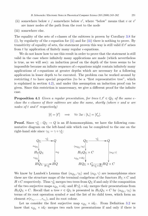
Proposition 4.1 Given a regular presentation, for trees t, t′ ∈ QΣ of the same ε-class the ε-classes of their subtrees are also the same, shortly (where v and w arenodes of t and t′ respectively)

[t] = [t′] =⇒ ∀v ∃w : [tv] = [t′w].

Proof. Since γ∗Σ : QΣ → Q is an H-homomorphism, we have the following com-

mutative diagram on the left-hand side which can be completed to the one on theright-hand side since γΣ = γ ◦ γ∗

Σ:

QΣ

αQΣ

��

γ∗Σ �� Q

αQ

��

HΣQΣ

εQΣ��

HQΣ Hγ∗Σ

�� HQ

QΣ

〈αQΣ,γΣ〉

��

γ∗Σ �� Q

〈αQ,γ〉

��

HΣQΣ × C

εQΣ×idC

��HQΣ × C

Hγ∗Σ×idC

�� HQ × C

We know by Lambek’s Lemma that 〈αQΣ, γΣ〉 and 〈αQ, γ〉 are isomorphisms since

these are the structure maps of the terminal coalgebras of the functors HΣ ×C andH×C respectively. Thus γ∗

Σ merges two trees from QΣ if and only if the compositionof the two surjective maps εQΣ

×idC and Hγ∗Σ×idC merges their presentations from

HΣQΣ × C. Recall that a tree r ∈ QΣ is presented in HΣQΣ × C by 〈αQΣ, γΣ〉 in

terms of its root operation symbol σ and the list of its child trees, which form anelement σ(rv1 , . . . , rvn), and its root colour.

Let us consider the first surjective map εQΣ× idC . From Definition 3.2 we

know that εQΣ× idC merges two such tree presentations if and only if there is


a corresponding ε-equation, i. e. one tree can be obtained from the other one viaan application of this ε-equation at the root. Since we assumed the equationalpresentation of H to be regular, εQΣ

only merges presentations for which the setsof all child trees are the same. This particularly means that for a pair of trees fromker((εQΣ

× idC) ◦ 〈αQΣ, γΣ〉) the ε-classes of the child trees are the same.

Now let us consider the second surjective map Hγ∗Σ × idC . Since 〈αQΣ

, γΣ〉 is anisomorphism and εQΣ

× idC is surjective, its domain HQΣ ×C is isomorphic to thequotient set of QΣ modulo the equivalence ker((εQΣ

× idC) ◦ 〈αQΣ, γΣ〉). And since

Hγ∗Σ × idC again is surjective, HQ is isomorphic to the quotient set of HQΣ × C

modulo the equivalence ker(Hγ∗Σ × idC). Taken together HQ (or equivalently, Q)

is isomorphic to the quotient set of QΣ modulo some equivalence R.If we can prove that R only contains pairs of trees whose child trees have the

same ε-classes, we easily get our proposition: since [t] = [t′], we have γ∗Σ(t) =

γ∗Σ(t′). We conclude from the above commutative diagram that the composition

of (εQΣ× idC) ◦ 〈αQΣ

, γΣ〉 and 〈αQ, γ〉−1 ◦ (Hγ∗Σ × idC) merges t and t′. This is

equivalent for t and t′ to form a pair in R, which implies that the child trees of t

and t′ have the same ε-classes. By structural induction on the trees this is also truefor arbitrary subtrees of t and t′.

In order to prove the desired property of R, we claim that

R = (ker((εQΣ× idC) ◦ 〈αQΣ

, γΣ〉) ∪ M)∗,

where

M := {(r, s)|αQΣ(r) = σ(rv1 , . . . , rvn), αQΣ

(s) = σ(sv1 , . . . , svn),[rvi ] = [svi ] for i = 1 . . . n and γΣ(r) = γΣ(s)}.

The star operation is the reflexive transitive closure and the set M contains all pairs(r, s) of trees where the root labels (operation symbol and colour) of r and s areequal and all their child trees at the same positions have the same ε-classes. Weprove our claim by showing the quotient set of QΣ modulo P := (ker((εQΣ

× idC) ◦〈αQΣ

, γΣ〉) ∪ M)∗ to be isomorphic to the codomain Q of γ∗Σ.

We first prove that all pairs of trees merged by γ∗Σ are contained in P : to be

merged by γ∗Σ means that the trees can be obtained from each other by an appli-

cation of ε-equations. But each sequence of applications of ε-equations is coveredby the construction of P : after applications of ε-equations at the root the pair iscontained in ker((εQΣ

× idC) ◦ 〈αQΣ, γΣ〉) ⊆ P . After (possibly infinitely many)

applications of ε-equations at depths ≥ 1 in a tree the corresponding pair of treeslies in P because it is contained in M . And an arbitrary combination of both ispossible due to the reflexive and transitive closure, thus the pair of the original treeand the resulting tree will always lie in P .

Conversely, assume a pair of trees to lie in P : this means that the pair arose bytransitivity from some pairs from ker((εQΣ

× idC) ◦ 〈αQΣ, γΣ〉) and from M . But

for these pairs we know that γ∗Σ merges the trees, and by transitivity of “having the

same ε-class” we conclude that γ∗Σ always merges the trees from a pair in P .


Finally it is an easy observation that R only contains pairs of trees whose childtrees have the same ε-classes: we already stated that for ker((εQΣ

×idC)◦〈αQΣ, γΣ〉)

and by definition it is also true for M and consequently for the union of both. Finallythe reflexive and transitive closure only adds pairs with the desired property because“having the same set of child tree ε-classes” is transitive. �

4.2 ε-classes and recolourings

Now we consider recolourings of trees. Unfortunately it is not true that for twotrees of the same ε-class the sets of all their recolourings are equal. To see this, wegive the following

Example 4.2 Let H be the finitary functor that is given as a quotient of HΣ =(−)2 +1 modulo the ε-equation σ(x, y) = σ(y, x) (Σ = {σ, c}, where σ is binary andc nullary). Since this equation is regular, H preserves preimages. Let C contain thecolours white and black. We consider the following coloured trees t and t′ from QΣ:

t :=

σ

σ

c c

σ

c c

t′ :=

σ

σ

c c

σ

c c

They obviously have the same ε-class [t] = [t′]. We obtain a recolouring r of t

by colouring the left-hand child of the root of t black. But now it is clear that thereis no recolouring of t′ that lies in the ε-class of r: in every recolouring of t′ bothchildren of the root must have the same colour because they are equivalent nodesin t′. But in every tree of the ε-class of r they have different colours, namely blackand white, because ε-equations preserve the colours of the nodes they are appliedto and the colourings of all subtrees of that node.

Nevertheless we can state a similar proposition for recolourings as we had forsubtrees (Proposition 4.1) if we restrict t to be a “first representative tree”, as weshall see.

Definition 4.3 Given a finitary functor H as a quotient of the polynomial functorHΣ and a linear order on Σ×C, we have a linear order (QΣ,≤) as mentioned in sec-tion 2.1. Then for every ε-class q ∈ Q we denote by tq ∈ QΣ the first representativetree of q. It is defined by [tq] = q and [t] = q ⇒ tq ≤ t for all t ∈ QΣ.

Remark 4.4 Given a linear order on Σ × C, the subset R ⊆ QΣ of first repre-sentative trees contains exactly one tree from each ε-class, which is clear from thedefinition. Additionally, R is closed under subtrees: we easily see that indeed everysubtree of such a first representative tree is a first representative tree of an ε-classagain. If there were some ε-equations that could be applied to a subtree such that


the result was a previous tree in the order, these applications of ε-equations hadshifted the whole tree to a previous position in the order.

For the rest of the paper when working with first representative trees we assumeΣ × C to be linearly ordered.

Example 4.5 In the case of LTS we have the presentation from Example 3.1 viathe polynomial functor

∑n∈N

(A×−)n. We can find a linear order where (σn, k) <

(σm, k) for every colour k and every two operations with arities n < m. The firstrepresentative trees we obtain are the strongly extensional trees as studied by JamesWorrell [12].

Now let us come back to the above Example 4.2. The reason that there is norecolouring of t′ in the ε-class of r is that the recolouring makes two subtrees of t

of the same ε-class become subtrees of r of different ε-classes. We can avoid this bychoosing a linear order on Σ×C and restricting t to be the first representative treetq of its ε-class q. In this case it follows from being the first representative tree (cf.Remark 4.4) that for any two subtrees of tq of the same ε-class their root nodes areequivalent. Since recolouring a tree preserves equivalent nodes, recolourings of firstrepresentative trees have the special property that any two subtrees of the sameε-class in the original tree become subtrees of the same ε-class in the recolouringagain. But note that recolourings of first representative trees in general are nolonger first representative trees.

Proposition 4.6 Given some q ∈ Q, for every tree t′ ∈ QΣ such that [t′] = q andevery recolouring r of tq there is a recolouring r′ of t′ such that [r] = [r′].

Proof. Given q and a recolouring r of tq, we will prove that

(1) a homomorphism f∗ : QΣ → QΣ can be defined such that r = f∗(tq) and

(2) [f∗(tq)] = [f∗(t′)] for all t′ with [t′] = q.

(1) Definition of f∗. The given recolouring r of tq yields a colour from C forevery subtree of tq, namely the colour r assigns to its root. Since tq is the firstrepresentative tree, all of its subtrees are first representative trees again. Thus thereis at most one subtree of tq from a given ε-class, namely the first representativetree of that ε-class. Furthermore, for possibly existing isomorphic subtrees theassignment always yields the same colour, see Remark 2.7. Then the colours of thesubtrees of tq given by r can be assigned to the ε-classes of these subtrees of tq in aunique way. More formally, let Stq ⊆ Q be the set of all ε-classes of subtrees of tq.Then r uniquely determines a C-colouring f ′′ : Stq → C of Stq .

Choosing arbitrary colours for the remaining ε-classes, we can extend f ′′ to aC-colouring f ′ : Q → C of Q. Using the map γ∗

Σ : QΣ → Q that assigns to everytree its ε-class, we extend f ′ to a C-colouring f : QΣ → C by defining f := f ′ ◦ γ∗

Σ.We obtain the homomorphism f∗ : QΣ → QΣ as the unique colour-compatiblehomomorphism (γΣ ◦ f∗ = f) into the cofree HΣ-coalgebra on C. We obviouslyhave f∗(tq) = r because for every subtree s of tq we have s ∈ γ∗

Σ−1(Stq) and the

root of f∗(s) is coloured with the colour f ′′ assigns to the ε-class of s.


(2) Proof of [f∗(tq)] = [f∗(t′)]. We consider a tree t′ with [t′] = q = [tq]. Recallfrom Theorem 3.6 that this is equivalent to ∂kt

q ∼ ∂kt′ for all k ∈ N. We want

to show by induction on the depth k of the cutting that ∂k(f∗(tq)) ∼ ∂k(f∗(t′)).Unfortunately we do not know how to prove that directly—what we actually dois to prove by induction on k that for all k ∈ N there is a tree tk for which thefollowing five statements hold.

(i) ∂k(tk) = ∂k(t′)

(ii) tk is obtained from tq by finitely many applications of ε-equations at depths< k

(iii) all subtrees of tk rooted at depths ≤ k have the same ε-classes as the corre-sponding subtrees of t′

(iv) f∗(tk) is obtained from f∗(tq) by application of the same ε-equations as theones used in (ii)

(v) ∂k(f∗(tk)) = ∂k(f∗(t′))

Then for every k we obtain ∂k(f∗(tq)) ∼ ∂k(f∗(t′)) from (iv) and (v) as follows:(iv) implies f∗(tq) ∼ f∗(tk). Since the ε-equations were only applied at depths< k and cutting at depth k preserves equivalent subtrees of depths < k, the same ε-equations witness ∂k(f∗(tq)) ∼ ∂k(f∗(tk)). Together with (v) we obtain ∂k(f∗(tq)) ∼∂k(f∗(t′)). Thus [f∗(t′)] = [f∗(tq)], and f∗(t′) is the required recolouring r′ of t′.Furthermore the induction proof is applicable to every tree t′ such that [t′] = [tq],and we finally obtain the proposition.

Now we prove by induction on k that for all k ∈ N there is a tree tk for whichthe statements (i) to (v) hold.

Base clause. For k = 0 we define t0 := tq. Then (ii) is directly clear from thedefinition (zero applications of ε-equations). We have (i) ∂0(t0) = ∂0(t′), becausethese are the root nodes of the trees tq and t′ respectively, which are labelled bythe same constant ⊥ and moreover have the same colour: by assumption they canbe obtained from each other by finitely many applications of (colour preserving) ε-equations. For (iii), there is nothing to prove. (iv) again is clear from the definitionof t0 (again zero applications of ε-equations). We prove (v) ∂0(f∗(t0)) = ∂0(f∗(t′)).Since ∂0 takes the root nodes of the trees and labels them with the constant ⊥, weonly have to show that the root colours of f∗(t0) and f∗(t′) are equal. But becauseof [t0] = [tq] = [t′], according to its definition f∗ colours both roots with the samecolour.

Induction step from k to k + 1. We assume that there is a tree tk such thatthe statements (i)k to (v)k hold. We then prove that these statements also hold fork + 1 instead of k, referred to as (i)k+1 to (v)k+1.

We claim that we can obtain a tree tk+1 which fulfills (i)k+1 and (iii)k+1 byapplication of (finitely many) ε-equations to tk at depth k. Then from (ii)k wedirectly get (ii)k+1. In fact one can obtain such a tree tk+1 that way:

From (i)k and (iii)k we know that we can obtain t′ by applications of (possiblyinfinitely many) ε-equations to tk at depths ≥ k. Additionally we know that, in


order to do so, we can first apply the (finitely many) ε-equations at depth k (withoutapplying equations in greater depths first) because any two nodes of tk at depthk+1 that could be made equivalent (by application of ε-equations in greater depths),already are equivalent—this is so because tq as a first representative tree has onlyfirst representative trees as subtrees and the application of regular ε-equations atdepths < k does not change subtrees rooted at depths ≥ k. After the applicationof all the ε-equations at depth k we can be sure that the subtrees of tk+1 rooted atdepth k + 1 have the same ε-classes as the corresponding subtrees of t′: ε-equationsthat were possibly applied at depths ≥ k + 1 before an ε-equation was applied atdepth k in the original chain of ε-equations did not change the ε-classes of subtreesrooted at depth k + 1, so looking only at the ε-classes, the ε-equation applied atdepth k rearranges subtrees at depth k + 1 in exactly the same way no matter ifapplied first or later. This proves (iii)k+1. This also ensures that the nodes of tk+1

at depth k + 1 have the same colours as the corresponding nodes of t′, becausetrees of the same ε-class always have the same root colour. And since the resultingoperation symbols at depth k are independent of when the ε-equations at depth k

are applied, we have (i)k+1.Next we prove (iv)k+1. It is sufficient to prove the commutativity of the following

diagram, then together with (iv)k we obtain (iv)k+1.

tkε-equations ��

f∗��

tk+1

f∗��

f∗(tk) same ε-equ.�� f∗(tk+1)

To do so, we first have to assert that the ε-equations used to obtain tk+1 fromtk are still applicable to the recolouring f∗(tk). This is indeed the case becausea recolouring does not change the tree shape and equivalent nodes of tk becomeequivalent nodes in the recoloured tree again. Second, both paths in the diagramresult in trees of the same shape: this is true because the ε-equations reshape tk andf∗(tk) the same way and the recolouring f∗ has no impact on the shape. Finally,both paths in the diagram lead to the same colouring (and thus the same tree): letus look at the nodes of depth k. The application of ε-equations to tk at depth k

preserves the ε-classes of the trees that are rooted at this depth and by its definitionf∗ consequently colours their roots the same way. Since the application of the sameε-equations to f∗(tk) at depth k preserves colours at this depth, at depth k we getthe same colours. The same argument can be used for nodes at depths < k. Theremaining nodes are these of depths > k, i. e. these of the subtrees rooted at depthk + 1. To them it does not matter whether they are rearranged by applications ofregular ε-equations at depth k first and then recoloured by f∗ or recoloured by f∗

first and then rearranged in the same way.Item (v)k+1 remains to be proven. By (i)k+1 we know that tk+1 and t′ have the

same shape down to depth k + 1 and by (iii)k+1 we know that all the ε-classes ofsubtrees rooted at depth ≤ k + 1 are the same for corresponding nodes of tk+1 andt′. Thus down to depth k + 1 corresponding nodes are recoloured by f∗ with the


same colour and we obtain ∂k+1(f∗(tk+1)) = ∂k+1(f∗(t′)). �

4.3 A simple coequational logic

Theorem 4.7 Let H be a finitary functor preserving preimages. For every linearorder on Σ×C the coequational logic of H has the following form: a coequation �q

is semantical consequence of the coequations �qi, i ∈ I, if and only if there is sometree r with [r] = qi for some i ∈ I, so that r is a recolouring of some subtree of tq,shortly ⋂

i∈I

�qi |= �q ⇐⇒ ∃i ∈ I ∃r.[r] = qi : r � tq. (4.1)

Proof. Since every finitary functor is accessible, from Theorem 2.11 we know thatthe left-hand side of (4.1) is equivalent to

∀t.[t] = q ∃i ∈ I ∃r.[r] = qi : r � t. (4.2)

We prove (4.2) to be equivalent to the right-hand side of (4.1).⇒ Since [tq] = q we can look at (4.2) in the special case of t = tq. It yields the

existence of a tree r such that [r] = qi for some i ∈ I and r � tq. Renaming r to r,this already is the right-hand side of (4.1).

⇐ From the right-hand side of (4.1) we have a tree r such that [r] = qi for somei ∈ I and r � tq. The latter means that r is a recolouring of some subtree s of tq.Proposition 4.1 yields for every tree t ∈ QΣ with [t] = q = [tq] the existence of asubtree s of t with [s] = [s]. Since s as a subtree of a first representative tree isagain a first representative tree, we obtain from Proposition 4.6 a recolouring r ofs with [r] = [r]. Altogether this means r � t and [r] = qi, which is exactly (4.2). �

Since for a semantical consequence of coequations the logic of Theorem 4.7 onlyrequires the existence of one tree r with some properties, it is much simpler thanthe logic for accessible functors of Theorem 2.11, which for each tree from a wholeε-class (such a class may contain infinitely many trees) requires the existence of atree r with these properties. Because of this (and using the fact that a subtree ofa first representative tree always is a first representative tree again) we are able toformulate two simple deduction rules similar to the case of polynomial functors.

Corollary 4.8 For systems of finitary functors that preserve preimages deductionof coequations with the following rules is sound and complete:

(i) child rule�q′

�qwhere tq

′is a child tree of tq

(ii) recolouring rule

�q′

�qwhere [r] = q′ for some recolouring r of tq


For an example of a logic given by Theorem 4.7, one may instantiate it with theLTS-functor Pf (A ×−) and an order as given in Example 4.5.

5 Finitary functors not preserving preimages

The first direction of Theorem 4.7 (completeness) was easily proven: nothing else butthe existence of first representative trees was needed, which is guaranteed for everyfinitary functor. But for the other way round (soundness) we needed some moreeffort, especially in Propositions 4.1 and 4.6, which are the core of the simpler logic:they guarantee that the simplification of section 4.3 works. In these propositionswe needed the assumption that the functor preserves preimages. We will now provethe necessity of this assumption for Theorem 4.7.

Theorem 5.1 A finitary functor H with |T | > 1 preserves preimages if and only iffor every linear order on Σ × C and any coequations �q and �qi, i ∈ I, we have:

⋂

i∈I

�qi |= �q ⇐⇒ ∃i ∈ I ∃r.[r] = qi : r � tq. (5.1)

Proof. In Theorem 4.7 for finitary functors preserving preimages it was shown thatfor every linear order on Σ × C and any coequations (5.1) is true. Now we assumea finitary functor H with |T | > 1 not to preserve preimages and find an order onΣ×C and coequations, for which (5.1) is not true. For this we do not need differentcolours, so in the following assume all trees to be coloured completely with the samecolour (or equivalently, think of uncoloured trees).

Since H does not preserve preimages, in every presentation of H there is anε-equation which is not regular, i. e. of the form

σ(x1, . . . , xn) = τ(y1, . . . , ym) (5.2)

where we have a non-empty set

Y := {yi | i ≤ m ∧ yi �= xj ∀j ≤ n}

of variables that do not appear on the left hand side. Moreover, we choose (5.2)such that these new variables yi ∈ Y appear as soon as possible when reading theτ -term from left to right. More precisely, we compare the τ -terms in their variablesfrom left to right asking whether the variables are contained in {x1, . . . , xn}. Assoon as a difference occurs, we choose the term that has the variable not containedin that set. Note that σ and τ may be the same operation symbol.

Now we denote by t the tree whose nodes are all labelled by σ, thus it has theproperty that all its subtrees are isomorphic to t itself. If the arity n ≥ 1 then t is atree where every path is infinite, if n = 0 (σ is a constant) then t is a singleton tree.In the ε-class [t] we can find all trees whose nodes are only labelled by the operationsσ and τ—this is because of (5.2): we can apply it to t, starting at the root andcontinuing until an arbitrary depth, exactly where we want a node to be labelled


by τ and we do not apply any ε-equation, where we want to keep the σ-labels. Forevery application of (5.2) we choose t for the variables from Y and ensure this waythat in greater depths we will always meet nodes labelled by σ.

Since the terminal coalgebra was assumed to have at least two elements, thereis a tree from an ε-class different from [t] (and this is not due to different colours).Consequently this tree has a node labelled by an operation ρ different from σ andτ . This operation ρ cannot be obtained at a node labelled with σ or τ applyingε-equations (in particular there are no ε-equations that equate ρ- and σ- or ρ- andτ -terms): if we could obtain ρ from σ or τ via (possibly many) ε-equations, we couldstate that directly in one ε-equation ρ(. . . ) = σ(. . . ) or ρ(. . . ) = τ(. . . ) because ofthe transitivity of ε-equations. But from this we derive analogously to the abovesituation for the ε-equation (5.2) that all trees with node labels from {ρ, τ, σ} belongto the same ε-class [t]. But then our assumption of an ε-class different from [t] wouldyield the existence of another operation different from ρ, τ and σ and so on; thatprocess only stops if we find an operation that cannot be obtained from one of theformer operations by application of ε-equations.

Now we consider a linear order of the operations in Σ such that the first onesare ρ < τ ≤ σ < . . . (which is turned into the beginning of an order of Σ × C byadding the single colour we are using in this proof). We consider the tree r whosenodes are all labelled by ρ. r is the first representative tree of its ε-class becauseρ is the first operation in the order. For its ε-class we have [r] �= [t] because thereare no ε-equations that could change ρ into σ. Now we evaluate (5.1) in the caseq := [t] and q0 := [r] (I = {0}).

We first show that the right-hand side of (5.1) is true: we find the tree tq fromthe ε-class q that is obtained from t by (in case n ≥ 1 infinitely many, but at everylevel finitely many) applications of (5.2) from left to right, starting at the rootof t and proceeding level by level applying it at every node that is root of a treeisomorphic to t. For variables from Y we use the tree r, and since Y is non-empty,r is subtree of tq of class q0. We show that tq is the first representative tree ofq: as mentioned there are no ε-equations whose application could replace τ by ρ

and as a consequence of the above assumption on (5.2) it is impossible to obtain apermutation of a node’s children such that ρ-labelled nodes shift to the left. Theseboth facts together with the chosen order of the operations ensures tq to be the firstrepresentative tree.

Second, we show that the left-hand side of (5.1) is not true: we just considerthe tree t from the ε-class q, whose nodes are all labelled by σ. It only has subtreesisomorphic to t which have the ε-class q �= q0; and recolourings of these subtreeswould have a different root colour than the single one we are using all the time andwhich is the root colour of all the trees from the ε-class q0. This means there is norecolouring of a subtree of t from the ε-class q0. �

5.1 Discussion

The intuition of the simpler logic is that the formation of ε-classes by γ∗Σ is com-

patible with subtrees and recolourings. We had to deal with both items in sections


4.1 and 4.2 respectively.Let us first recall from Proposition 4.1 what compatibility of ε-classes and sub-

trees means: whenever two Σ-trees are merged in one ε-class, their direct subtreesare merged in ε-classes again, and recursively for all their subtrees. The consequenceof this is that with knowing one tree of an ε-class one already knows the ε-classesof the subtrees of all other trees of this class, what is captured by the quantifiers(exists / for all) in the above formulas. Finitary functors H that preserve preimagesensure that compatibility of ε-classes and subtrees by their homomorphisms (γ∗

Σ isan H-homomorphism); all other finitary functors do not: as seen in the proof ofTheorem 5.1 trees can be merged in one ε-class without their subtrees having thesame ε-classes.

Now let us have a look at compatibility of ε-classes and recolourings. Theseconcepts just are not compatible: having ε-classes means having different trees inthese ε-classes. But as long as subtrees of a tree are not isomorphic, what wouldbe respected by recolourings, arbitrary recolourings can be applied to them takingthem to different ε-classes. And since we surely have some trees with and some treeswithout isomorphic subtrees, more or less recolourings can be applied and more orless ε-classes can be obtained as seen in Example 4.2. To solve these problemswe hid the complexity of ε-classes by their first representative trees. In these firstrepresentative trees “as much subtrees as possible” are isomorphic and this waythe recolourings of a first representative tree form a “minimal” set of ε-classes.Under the additional assumption of a preimage preserving functor it turns out inProposition 4.6 that for every tree of the ε-class of a given first representative tree therecolourings form a superset of this set. And this is enough compatibility of ε-classesand recolourings to state our simple logic, now working with first representativetrees.

6 Deduction of Sets

For semantical consequences of arbitrary subsets of the cofree coalgebra of a poly-nomial functor there is the following statement.

Theorem 6.1 ([1]) Let U, U ′ ⊆ QΣ be arbitrary subsets of the cofree HΣ-coalgebraof a polynomial functor HΣ. The following holds: U is semantical consequence ofU ′, if and only if every t ∈ QΣ, for which all recolourings of all subtrees lie in U ′,is contained in U , shortly

U ′ |= U ⇐⇒ ∀t ∈ QΣ : (∀r.r � t : r ∈ U ′) ⇒ t ∈ U .

Analogously to that statement we can prove one for the case of accessible functorsalthough this was not expected by [1].

Theorem 6.2 Let U ′, U ⊆ Q be arbitrary subsets of the cofree H-coalgebra of anaccessible functor H. The following holds: U is semantical consequence of U ′, ifand only if every ε-class q ∈ Q, in which there exists a tree t ∈ QΣ, for which the


ε-classes of all recolourings of subtrees of t lie in U ′, lies in U , shortly

U ′ |= U ⇐⇒ ∀q ∈ Q : (∃t.[t] = q ∀r.r � t : [r] ∈ U ′) ⇒ q ∈ U .

Proof. We give a proof analogously to the one of [1] for Theorem 6.1. First wereduce semantical consequences of sets to semantical consequences of coequationsproving

U ′ |= U ⇐⇒ ∀q ∈ Q : (U |= �q) ⇒ (U ′ |= �q).

To do so, recall from section 2.2 that U ⊆ Q is logically equivalent to a set ofcoequations �qi, i ∈ I where

⋃i∈I qi is the complement of U . From U ′ |= U and

U |= �q we immediately have U ′ |= U |= �q and consequently U ′ |= �q due totransitivity of |=. On the other hand, if we assume (U |= �q) ⇒ (U ′ |= �q) for allq ∈ Q, in particular we have (U |= �qi) ⇒ (U ′ |= �qi) for all i ∈ I. Since U |= �qi

is always true for all i ∈ I, it holds that U ′ |= �qi for all i ∈ I. But this just meansU ′ |= U .

Now we can apply Theorem 2.11 in order to get an expression for semanticalconsequences of sets in terms of the relation �. Afterwards we use the logicalequivalence a ⇒ b ≡ ¬b ⇒ ¬a to rewrite that expression:

(U |= �q) ⇒ (U ′ |= �q)⇐⇒ (∀t∃r∃qi ∈ Q \ U : [t] = q ⇒ [r] = qi ∧ r � t)

⇒ (∀t∃r∃qi ∈ Q \ U ′ : [t] = q ⇒ [r] = qi ∧ r � t)⇐⇒ (∃t∀r∀qi ∈ Q \ U ′ : [t] = q ∧ ([r] �= qi ∨ r �� t))

⇒ (∃t∀r∀qi ∈ Q \ U : [t] = q ∧ ([r] �= qi ∨ r �� t))

By slightly rewriting the premise of the latter formula (line before last) we see thatit is exactly the premise in the theorem because ∀qi ∈ Q \ U ′ : [r] �= qi just means[r] ∈ U ′. But the conclusion of the formula (last line) is the conclusion in thetheorem, too: in the special case r = t we get ∃t∀qi ∈ Q \ U : [t] = q ∧ [t] �= qi,what means q ∈ U . On the other hand, we cannot conclude anything else from theformula but q′ ∈ U for some ε-class q′; this is covered by the for all quantifier for q

in the theorem. �

7 Conclusion and future work

In the present paper we formulated a simple coequational logic for preimage pre-serving finitary functors and proved it to be sound and complete. We also provedthat in general we cannot obtain this simple coequational logic for finitary functorsthat do not preserve preimages. Finally we proved a theorem for accessible func-tors that makes explicit what are semantical consequences of arbitrary subsets of acofree coalgebra.

It would be of interest to look at infinitary accessible functors. In this casefunctors may preserve preimages but have no regular presentation, and the questionarises which of both is the property needed to establish a simple logic (if this is


still possible at all). We conjecture that the regular presentation is the importantproperty since in our paper we never needed to consider a preimage.

References

[1] Adamek, J., A logic of coequations, in: L. Ong, editor, Computer Science Logic – Proceedings of the19th International Workshop, LNCS 3634 (2005), pp. 70–86.

[2] Adamek, J., D. Lucke and S. Milius, Recursive coalgebras of finitary functors, Theoretical Informaticsand Applications (2007).

[3] Adamek, J. and S. Milius, Terminal coalgebras and free iterative theories, Information and Computation204 (2006), pp. 1139–1172.

[4] Adamek, J. and H.-E. Porst, On tree coalgebras and coalgebra presentations, Theoretical ComputerScience 311 (2004), pp. 257–283.

[5] Adamek, J. and V. Trnkova, “Automata and Algebras in Categories,” Kluwer Academic Publishers,1990.

[6] Gumm, H. P., Elements of the general theory of coalgebras, LUATCS ’99, Rand Afrikaans University,Johannesburg, South Africa (1999).

[7] Hughes, J., Modal operators for coequations, in: Coalgebraic Methods in Computer Science (CMCS’01),Electronical Notes in Theoretical Computer Science 44.1, 2001, pp. 204–225.

[8] Moss, L. S., Coalgebraic logic, Annals of Pure and Applied Logic 96 (1999), pp. 177–317.

[9] Pattinson, D., Coalgebraic modal logic: soundness, completeness and decidability, Theoretical ComputerScience 309 (2003), pp. 177–193.

[10] Rutten, J. J. R. R., Universal coalgebra: a theory of systems, Theoretical Computer Science 249 (2000),pp. 3–80.

[11] Schwencke, D., “Coalgebraische Logik von markierten Transitionssystemen,” Master’s thesis, TechnicalUniversity, Braunschweig (2007), unpublished.

[12] Worrell, J., On the final sequence of a finitary set functor, Theoretical Computer Science 338 (2005),pp. 184–199.


coequational logic for finitary functors

Documents