coe/res discussion paper series, no - econ.hit-u.ac.jpcoe-res/dp_doc/no_194_dp.pdf · coe-res...
TRANSCRIPT

COE-RES Discussion Paper Series Center of Excellence Project
The Normative Evaluation and Social Choice of Contemporary Economic Systems
Graduate School of Economics and Institute of Economic Research Hitotsubashi University
COE/RES Discussion Paper Series, No.194 December 2006
Choice, Opportunities, and Procedures: Collected Papers of Kotaro Suzumura
Part I Rational Choice and Revealed Preference
Kotaro Suzumura (Hitotsubashi University)
Naka 2-1, Kunitachi, Tokyo 186-8603, Japan Phone: +81-42-580-9076 Fax: +81-42-580-9102
URL: http://www.econ.hit-u.ac.jp/~coe-res/index.htmE-mail: [email protected]

Choice, Opportunities, and Procedures:
Collected Papers of Kotaro Suzumura
Part I Rational Choice and Revealed Preference
Kotaro Suzumura
Institute of Economic Research, Hitotsubashi UniversityKunitatchi, Tokyo 186-8603, Japan
December 25, 2006

Table of Contents
Introduction
Part I Rational Choice and Revealed PreferenceChapter 1 Rational Choice and Revealed Preference
Chapter 2 Houthakker’s Axiom in the Theory of Rational Choice
Chapter 3 Consistent Rationalizability
Chapter 4 Rationalizability of Choice Functions on General Domains Without Full Transitivity
Part II Equity, Efficiency, and SustainabilityChapter 5 On Pareto-Efficiency and the No-Envy Concept of Equity
Chapter 6 The Informational Basis of the Theory of Fair Allocations
Chapter 7 Ordering Infinite Utility Streams
Chapter 8 Infinite-Horizon Choice Functions
Part III Social Choice and Welfare EconomicsChapter 9 Impossibility Theorems without Collective Rationality
Chapter 10 Remarks on the Theory of Collective Choice
Chapter 11 Paretian Welfare Judgements and Bergsonian Social Choice
Chapter 12 Arrovian Aggregation in Economic Environments: How Much Should We KnowAbout Indifference Surfaces?
Part IV Individual Rights and Social WelfareChapter 13 On the Consistency of Libertarian Claims
Chapter 14 Liberal Paradox and the Voluntary Exchange of Rights-Exercising
Chapter 15 Individual Rights Revisited
Chapter 16 Welfare, Rights, and Social Choice Procedure: A Perspective
Part V Competition, Cooperation and Economic WelfareChapter 17 Entry Barriers and Economic Welfare
Chapter 18 Oligopolistic Competition and Economic Welfare: A General Equilibrium Analysisof Entry Regulation and Tax-Subsidy Schemes
Chapter 19 Cooperative and Noncooperative R&D in Oligopoly with Spillovers
Chapter 20 Symmetric Cournot Oligopoly and Economic Welfare: A Synthesis
Part VI Consequentialism versus Non-consequentialismChapter 21 Consequences, Opportunities, and Procedures
Chapter 22 Characterizations of Consequentialism and Non-Consequentialism
Chapter 23 Consequences, Opportunities, and Generalized Consequentialism and Non-Conse-quentialism

Chapter 24 Welfarist-Consequentialism, Similarity of Attitudes, and Arrow’s General Impos-sibility Theorem
Part VII Historically SpeakingChapter 25 Introduction to Social Choice and Welfare
Chapter 26 Between Pigou and Sen: Pigou’s Legacy, Hicks’ Manifesto, and Non-WelfaristicFoundations of Welfare Economics
Chapter 27 An Interview with Paul Samuelson: Welfare Economics, ‘Old’ and ‘New’, andSocial Choice Theory
Chapter 28 An Interview with Kenneth J. Arrow: Social Choice and Individual Values

Original Sources
Part I
Chapter 1: “Rational Choice and Revealed Preference,”Review of Economic Studies, Vol.43, 1976,pp.149-158.
Chapter 2: “Houthakker’s Axiom in the Theory of Rational Choice,” Journal of Economic Theory,Vol.14, 1977, pp.284-290.
Chapter 3: “Consistent Rationalizability,” Economica, Vol.72, 2005, pp.185-200. Joint paper withW. Bossert and Y. Sprumont.
Chapter 4: “Rationalizability of Choice Functions on General Domains Without Full Transitivity,”Social Choice and Welfare, Vol.27, 2006, pp.435-458. Joint paper with W. Bossert and Y.Sprumont.
Part II
Chapter 5: “On Pareto-Efficiency and the No-Envy Concept of Equity,” Journal of Economic Theory,Vol.25, 1981, pp.367-379.
Chapter 6: “The Informational Basis of the Theory of Fair Allocation,”Social Choice and Welfare,Vol.24, 2005, pp.311-341. Joint paper with M. Fleurbaey and K. Tadenuma.
Chapter 7: “Ordering Infinite Utility Streams,” forthcoming in Journal of Economic Theory . Jointpaper with W. Bossert and Y. Sprumont.
Chapter 8: “Infinite-Horizon Choice Functions,” Working Paper, University of Montreal. Joint Paperwith G. Asheim, W. Bossert and Y. Sprumont.
Part III
Chapter 9: “Impossibility Theorems without Collective Rationality,” Journal of Economic Theory,Vol.13, 1976, pp.361-379. Joint paper with D. H. Blair, G. Bordes and J. S. Kelly. Reprinted inK. J. Arrow and G. Debreu, eds., The Foundations of 20th Century Economics, Vol.3, LandmarkPapers in General Equilibrium Theory, Social Choice and Welfare, Cheltenham, Glos.: EdwardElgar, 2001, pp.660-678.
Chapter 10: “Remarks on the Theory of Collective Choice,” Economica, Vol.43, 1976, pp.381-390.
Chapter 11: “ParetianWelfare Judgements and Bergsonian Social Choice,” Economic Journal, Vol.109,1999, pp.204-220. Reprinted in J. C. Wood and M. McLure, eds., Paul A. Samuelson: Crit-ical Assessments of Contemporary Economists, Vol.2, 2nd Series, London: Routledge, 2004,pp.378-396.
Chapter 12: “Arrovian Aggregation in Economic Environments: How Much Should We Know AboutIndifference Surfaces?” Journal of Economic Theory, Vol.124, 2005, pp.22-44. Joint Paper withM. Fleurbaey and K. Tadenuma.

Part IV
Chapter 13: “On the Consistency of Libertarian Claims,” Review of Economic Studies, Vol.45, 1978,pp.329-342. “A Correction,” Review of Economic Studies, Vol.46, 1979, p.743.
Chapter 14: “Liberal Paradox and the Voluntary Exchange of Rights-Exercising,” Journal of Eco-nomic Theory, Vol.22, 1980, pp.407-422. Reprinted in C. K. Rowley, ed., The InternationalLibrary of Critical Writings in Economics, Vol.27, Social Justice and Classical Liberal Goals,Cheltenham, Glos.: Edward Elgar, 1993, pp.483-498.
Chapter 15: “Individual Rights Revisited,” Economica, Vol.59, 1992, pp.161-177. Joint paper withW. Gaertner and P. K. Pattanaik. Reprinted in C. K. Rowley, ed., The International Library ofCritical Writings in Economics, Vol.27, Social Justice and Classical Liberal Goals, Cheltenham,Glos.: Edward Elgar, 1993, pp.592-608.
Chapter 16: “Welfare, Rights, and Social Choice Procedure: A Perspective,”Analyse & Kritik, Vol.18,1996, pp.20-37.
Part V
Chapter 17: “Entry Barriers and Economic Welfare,” Review of Economic Studies, Vol.54, 1987,pp.157-167. Joint paper with K. Kiyono.
Chapter 18: “Oligopolistic Competition and Economic Welfare: A General Equilibrium Analysisof Entry Regulation and Tax-Subsidy Schemes,” Journal of Public Economics, Vol.42, 1990,pp.67-88. Joint paper with H. Konishi and M. Okuno-Fujiwara.
Chapter 19: “Cooperative and Noncooperative R&D in Oligopoly with Spillovers,” American Eco-nomic Review, Vol.82, 1992, pp.1307-1320.
Chapter 20: “Symmetric Cournot Oligopoly and Economic Welfare: A Synthesis,” Economic Theory,Vol.3, 1993, pp.43-59. Joint paper with M. Okuno-Fujiwara.
Part VI
Chapter 21: “Consequences, Opportunities, and Procedures,” Social Choice and Welfare, Vol.16,1999, pp.17-40.
Chapter 22: “Characterizations of Consequentialism and Non-Consequentialism,” Journal of Eco-nomic Theory, Vol.101, 2001, pp.423-436. Joint paper with Y. Xu.
Chapter 23: “Consequences, Opportunities, and Generalized Consequentialism and Non-Conse-quentialism,” Journal of Economic Theory, Vol.111, 2003, pp.293-304. Joint paper with Y. Xu.
Chapter 24: “Welfarist-Consequentialism, Similarity of Attitudes, and Arrow’s General ImpossibilityTheorem,” Social Choice and Welfare, Vol.22, 2004, pp.237-251. Joint paper with Y. Xu.
Part VII
Chapter 25: “Introduction to Social Choice and Welfare,” in K. J. Arrow, A. K. Sen and K. Suzumura,eds., Handbook of Social Choice and Welfare, Vol.I, Amsterdam: Elsevier, 2002, pp.1-32.

Chapter 26: “Between Pigou and Sen: Pigou’s Legacy, Hicks’ Manifesto, and Non-Welfaristic Foun-dations of Welfare Economics,” forthcoming in R. E. Backhouse and T. Nishizawa, eds., NoWealth but Life: The Origins of Welfare Economics and the Welfare State in Britain.
Chapter 27: “An Interview with Paul Samuelson: Welfare Economics, ‘Old’ and ‘New’, and SocialChoice Theory,” Social Choice and Welfare, Vol.25, 2005, pp.327-356.
Chapter 28: “An Interview with Kenneth Arrow: Social Choice and Individual Values,” forthcomingin K. J. Arrow, A. K. Sen and K. Suzumura, eds., Handbook of Social Choice and Welfare, Vol.II,Amsterdam: Elsevier Science B. V.

Introduction
Kotaro Suzumura’s work are mostly in the area of welfare economics and social choice
theory. His work in the area of theoretical industrial organization, as well as his policy-
oriented work on industrial policy, competition policy, and development policy, are deriva-
tives from his work on welfare economics and social choice theory. This collection of his
selected papers gathers his representative contributions in the major area of research,
which are classified in seven parts.
The first part focuses on the axiomatic characterization of the concept of rational
choice as purposive action. It was Lionel Robbins who first crystallized this classical
notion of rationality, which Paul Samuelson elaborated into the celebrated edifice of
revealed preference theory. Capitalizing on the contributions by Paul Samuelson, Hen-
drik Houthakker, Kenneth Arrow, Marcel Richter, Bengt Hansson, and Amartya Sen,
Suzumura contributed to the axiomatic characterization of rational choice on the gen-
eral domain. As an auxiliary step, Suzumura generalized Szpilrajn’s classical extension
theorem on binary relations in terms of his newly introduced concept of consistency. Con-
sistency of a binary relation requires any preference cycle to involve indifference only. As
shown by Suzumura, consistency is necessary and sufficient for the existence of an order-
ing extension of a binary relation. This novel concept of consistency and the generalized
extension theorem are playing a basic role in this and many other contexts of choice and
preference. This part contains Suzumura’s basic contributions along these lines.
The second part focuses on the logical conflict between equity and efficiency in several
distinct contexts. Generalizing the early contributions by Serge Kolm, Duncan Foley, and
Hal Varian, which may be traced back even further to John Hicks and Jan Tinbergen,
Suzumura contributed to build a bridge between the theory of fairness and the theory
of social choice, thereby enriching both theories and clarifying their logical relationships.
This assertion is substantiated by the first two papers in this part. There is another and
even more classical concept of equity, which was introduced by Henry Sidgwick in the
context of treating different generations equitably. The last two papers in this part are
Suzumura’s recent work on the possibility of ordering infinite utility streams on the basis
of intergenerational equity and intertemporal efficiency.
The third part focuses on the Arrovian impossibility theorems in social choice theory.
Arrow’s original formulation of the problem of social choice was in terms of the social
welfare function, the maximization of which subject to the feasibility constraints was
construed to be the task of the social decision-maker. An early work of Suzumura in

this arena was to see how Arrow’s impossibility theorem fares if we get rid of the social
welfare function and focus directly on the social choice per se. One of his more recent
work in this arena asked how the Arrovian impossibility theorem fares if we treat an
explicitly economic environment and weaken Arrow’s axiom of independence of irrelevant
alternatives by allowing richer information about individual preferences. This part also
contains a paper in which the crucial concept of coherence was first introduced, and
another paper on the logical relations between the compensation principles a la Kaldor,
Hicks, Scitovsky and Samuelson, on the one hand, and the Bergson-Samuelson social
welfare function, on the other.
The fourth part focuses on the logical coherence between social welfare and individual
rights. It was Amartya Sen who posed the problem of compatibility of these two essential
values in social choice, which he crystallized into the justly famous impossibility of a
Paretian liberal . Suzumura’s contribution in this arena is two-hold. In the first place,
he could identify several escape routes from Sen’s impasse, keeping Sen’s formulation
of individual rights in terms of individual decisiveness in social choice intact. In the
second place, he came to the important recognition that Sen’s original articulation of
libertarian rights is incompatible with the classical concept of freedom of choice a la
John Stuart Mill, and contributed to develop an alternative game-form articulation of
individual rights. This part contains some of his representative contributions along these
lines.
The fifth part focuses on the welfare effect of increasing competitiveness and interfirm
collaboration. Contrary to the widespread and classical belief in competition as an effi-
cient and decentralized mechanism for allocating resources, Suzumura proved what came
to be called the excess entry theorem to the effect that the free-entry number of firms in
the Cournot oligopoly market is socially excessive vis-a-vis the first-best number of firms
as well as the second-best number of firms. This and related work motivated him to dig
much deeper into the relationship between welfare, competition and collaboration. This
part contains his major contributions in this area of research.
The sixth part focuses on the intrinsic, rather than instrumental, value of opportu-
nities for making choice and procedures for decision-making. The inquiry along this line
led Suzumura to go beyond consequentialism, which had remained almost unchallenged
in the literature. He could obtain an axiomatic characterization of consequentialism and
non-consequentialism, as well as some clarifications of the effects of going beyond con-
sequentialism on such standard result as Arrow’s general impossibility theorem in the
theory of social choice.

The seventh part focuses on the analytical history of welfare economics. Although
the nomenclature of welfare economics should be attributed to Arthur Pigou for his
celebrated classic, The Economics of Welfare, the history of welfare economics could be
traced back at least as far as to Adam Smith and Jeremy Bentham, and possibly further
beyond Adam Smith, under the classical nomenclature of moral philosophy. Suzumura’s
work in this arena crystallize some of the crucial steps in the historical evolution of welfare
economics, paying due attention to the informational basis of social welfare judgements,
and the intrinsic value of social decision-making procedures and opportunities to choose.
This part also contains two interviews with the great pioneers in the development of
welfare economics and social choice theory, viz., Paul Samuelson and Kenneth Arrow.

Chapter 1Rational Choice and Revealed Preference∗
1 Introduction
According to the currently dominant view, the choice behaviour of an agent is construedto be rational if there exists a preference relation R such that, for every set S of availablestates, the choice therefrom is the set of “R-optimal” points in S.1 There are at least twoalternative definitions of R-optimality—R-maximality and R-greatestness. On the onehand, an x in S is said to be R-maximal in S if there exists no y in S which is strictlypreferred to x in terms of R. On the other, an x in S is said to be R-greatest in S if, forall y in S, x is at least as preferable as y in terms of R. The former viewpoint can claimits relevance in view of the prevalent adoption of the concept of Pareto-efficiency in thetheory of resource allocation processes.2 The latter standpoint is deeply rooted in thewell-developed theories of the integrability problem, revealed preference and social choice.The difference between these two definitions of rational choice is basically as follows. Anytwo states in a choice function which is R-maximal rational are either R-indifferent orR-incomparable, while any two states in a choice function which is R-greatest rationalare R-indifferent.
A condition for rational choice has been put forward in terms of the R-greatestnessinterpretation of optimality (Hansson [4] and Richter [9, 10]). In this chapter, a conditionfor rational choice in its R-maximality interpretation will be presented. The conditionin question will, in a certain sense, synthesize both concepts of rationality, because itcan be seen that the rational choice in terms of R-maximality is rational in terms ofR-greatestness as well. The role of various axioms of revealed preference and congruencein the theory of rational choice will also be clarified.
∗First published in Review of Economic Studies, Vol.43, 1976, pp.149-158. Thanks are due to theeditors of this journal for their helpful comments on the earlier version of this chapter.
1Arrow’s seminal works [1, 2] are the main sources of the current theory of rational choice. Notablecontributions in this field include Hansson [4], Richter [9, 10] and Sen [13], among others. See alsoHerzberger [5], Jamison and Lau [7] and Wilson [16]. In his recent paper [8], Plott axiomatized theconcept of path-independent choice which is related to, but distinct from, the concept of rational choice.See Suzumura [15].
2See also Herzberger [5, pp.196-199], who calls an agent a liberal maximizer [resp. stringent maxi-mizer ], if he chooses R-maximal points [resp. R-greatest points] from the points available and favoursthe liberal maximizer as a model of rational agent.
1
In this kind of analysis, special care should be taken with the domain of the choicefunction. It was Arrow [1] who first suggested that “the demand-function point of viewwould be greatly simplified if the range over which the choice functions are considered tobe determined is broadened to include all finite sets”. This line of enquiry was recentlycompleted by Sen [13].3 It is true, as was persuasively discussed by Sen [13, Section 6],that there is no convincing reason for our restricting the domain of the choice functionto the class of convex polyhedras representing budget sets in the commodity space. Atthe same time, however, it should be admitted that there exists no specific reason for ourextending the domain so as to include all finite sets. This being the case, no restrictionwhatsoever will be placed on the domain of the choice function in this chapter exceptthat it should be a non-empty family of non-empty sets.
In Section 2, our conceptual framework will be presented. The main results will bestated in Section 3, the proofs thereof being given in Section 4. In Section 5 we willpresent some examples which will negate the converse of our theorems. Finally, Section6 will be devoted to comparing our results with the Arrow-Sen theory, on the one hand,and the Richter-Hansson theory, on the other.
2 Definitions
Let X be the basic set of all alternatives and let K stand for the non-empty family ofnon-empty subsets of X. A suggested interpretation is that each and every S ∈ K is theset of available alternatives which could possibly be presented to the agent. For the sakeof brevity, a series of formal definitions will be given below.
Definition 1 (Preference Relation): A preference relation is a binary relation R on X,that is to say, a subset of X ×X. If (x, y) ∈ R, we say that x is at least as preferable asy. A strict preference relation associated with R is a binary relation
PR = (x, y) ∈ X ×X|(x, y) ∈ R & (y, x) /∈ R.
An indifference relation associated with R is a binary relation
IR = (x, y) ∈ X ×X|(x, y) ∈ R & (y, x) ∈ R.
R is said to be
(a) complete iff (x, y), (y, x) ∩R 6= ∅ for all x, y ∈ X,(b) acyclic iff (x, x) /∈ T (PR) for all x ∈ X,4
(c) transitive iff [(x, y) ∈ R & (y, z) ∈ R ⇒ (x, z) ∈ R] for all x, y, z ∈ X, and
3As was carefully noted by Sen [13, p.312], the Arrow-Sen theory works well even if the domainincludes all pairs and all triples, but not all finite sets.
4For any binary relation Q on X, T (Q) stands for the transitive closure of Q: T (Q) = (x, y) ∈X ×X|(x, y) ∈ Q or [(x, z1), (zk, zk+1), (zn, y) ∈ Q (k = 1, . . . , n− 1) for some z1, . . . , zn ⊂ X]. If Ris acyclic, there exists no strict preference cycle.
2

(d) an ordering iff it is complete as well as transitive.
Definition 2 (Maximal-Point Set and Greatest-Point Set): Let R and S be, respec-tively, a preference relation and an arbitrary subset of X. The subsets M(S, R) andG(S, R) of S, to be called the R-maximal-point set and the R-greatest-point set of S,respectively, are defined by
M(S,R) = x ∈ X|x ∈ S & (y, x) /∈ PR for all y ∈ S
andG(S, R) = x ∈ X|x ∈ S & (x, y) ∈ R for all y ∈ S.
Remark 1. (i) For any S ⊂ X and R ⊂ X ×X, G(S,R) ⊂ M(S, R), and (ii) if R iscomplete, G(S, R) = M(S,R).5 For any x, y ∈ G(S,R), we have (x, y) ∈ IR, while forany x, y ∈ M(S, R), we have either (x, y) ∈ IR or [(x, y) /∈ R & (y, x) /∈ R].
Definition 3 (Choice Function): A choice function is a function C on K such thatC(S) is a non-empty subset of S for all S ∈ K.
The intended interpretation is that, for any set S of available alternatives, the subsetC(S) thereof represents the set of alternatives which are chosen from S. Associated withthe given choice function C on K, we can define various concepts of revealed preference.
Definition 4 (Revealed Preference Relations): Two preference relations R∗ and R∗ onX such that
(a)(x, y) ∈ R∗ iff [x ∈ C(S) & y ∈ S] for some S ∈ K, and(b)(x, y) ∈ R∗ iff [x /∈ S or x ∈ C(S) or y /∈ C(S)] for all S ∈ K
are called the revealed preference relations .
In words, x is said to be revealed R∗-preferred to y if x is chosen when y is also avail-able, and x is said to be revealed R∗-preferred to y if there exists no choice situation inwhich y is chosen and x is available but rejected. In order to connect these revealed pref-erence relations to the revealed preference axioms, we introduce the following auxiliaryconcept.
Definition 5 (C-connectedness): A sequence of sets (S1, . . . , Sn) in K is said to beC-connected iff Sk ∩ C(Sk+1) 6= ∅ for all k ∈ 1, . . . n− 1 and Sn ∩ C(S1) 6= ∅.
It turns out that for our present purpose the following rather abstract formulation ofthe revealed preference axioms is the most convenient.
Definition 6 (Revealed Preference Axioms): A choice function C on K is said tosatisfy
5For the proof of this well-known result, see Herzberger [5, Proposition P1] and Sen [12, Chapter 1∗].
3

(a)Weak Axiom of Revealed Preference — (WARP), for short — iff for any C-connected pair (S1, S2) in K, S1 ∩ C(S2) = C(S1) ∩ S2 holds,
(b)Strong Axiom of Revealed Preference — (SARP), for short — iff for any C-connected sequence (S1, . . . , Sn) in K, Sk ∩ C(Sk+1) = C(Sk) ∩ Sk+1 for somek ∈ 1, . . . , n− 1 holds, and
(c)Hansson’s Axiom of Revealed Preference — (HARP), for short — iff for anyC-connected sequence (S1, . . . , Sn) in K, Sk ∩ C(Sk+1) = C(Sk) ∩ Sk+1 for allk ∈ 1, . . . , n− 1.
At first sight, (WARP) and (SARP) in Definition 6, which are due originally toHansson [4], might seem rather different from their traditional formulation, such as inSen [13], but they are equivalent. In order to substantiate this claim, let us define anotherrevealed preference relation R∗∗ by (x, y) ∈ R∗∗ iff [x ∈ C(S) & y ∈ S\C(S)] for someS ∈ K. By definition, we have R∗∗ ⊂ R∗. (In words, x is said to be revealed R∗∗-preferredto y if x is chosen and y is available but rejected.) In terms of R∗ and R∗∗, the commonversion of (WARP) is given by:
(x, y) ∈ R∗∗ ⇒ (y, x) /∈ R∗. (1)
Similarly, the traditional formulation of (SARP) is given by:
(x, y) ∈ T (R∗∗) ⇒ (y, x) /∈ R∗. (2)
It will be shown in the Appendix that (1) and (2) are equivalent to (WARP) and (SARP),respectively, in Definition 6.
We are now in the position to introduce the concepts coined by Richter [9] and Sen[13].
Definition 7 (Congruence Axioms): A choice function C on K is said to satisfy
(a)Weak Congruence Axiom — (WCA), for short — iff for any S ∈ K, (x, y) ∈ R∗,x ∈ S and y ∈ C(S) imply x ∈ C(S), and
(b)Strong Congruence Axiom — (SCA), for short — iff for any S ∈ K, (x, y) ∈ T (R∗),x ∈ S and y ∈ C(S) imply x ∈ C(S).
The central concepts of this paper are given by the following definition.
Definition 8 (Rational Choice Function): A choice function C on K is said to be
(a)G-rational iff there exists a preference relation R such that C(S) = G(S, R) forall S ∈ K, and
(b)M-rational iff there exists a preference relation R such that C(S) = M(S, R) forall S ∈ K.
4

A preference relation R which rationalizes the choice function C is called the ratio-nalization of C.6
Intuitively, a choice function is said to be rational if we can interpret the stipulatedchoice behaviour as a kind of preference optimization. Two possible interpretations ofthis idea are formulated in Definition 8(a) and (b). It should be noted that the M-rationalchoice function is G-rational but not vice versa. This can be seen as follows. Let C onK be M -rational with the rationalization R. We define a binary relation R′ on X by[(x, y) ∈ R′ ⇔ (y, x) /∈ PR] for all x and y in X. From Definition 2, we then haveM(S, R) = G(S,R′) for all S ∈ K, so that C is G-rational with the rationalization R′.In order to see that the G-rational choice function is not necessarily M -rational, let usconsider an example where X = x, y, z, K = S1, S2, S3, S1 = x, y, S2 = x, z, S3 =X,C(S1) = S1, C(S2) = S2 and C(S3) = x. This choice function is G-rational with therationalization R = (x, y), (y, x), (x, z), (z, x). Assume that this C is M -rational withthe rationalization R′. From C(S1) = S1 we obtain:
(x, y) ∈ IR′ or [(x, y) /∈ R′ & (y, x) /∈ R′] (3)
From C(S2) = S2 we obtain:
(x, z) ∈ IR′ or [(x, z) /∈ R′ & (z, x) /∈ R′] (4)
From C(S3) = x we obtain:
[(x, y) ∈ PR′ or (z, y) /∈ PR′ ] & [(x, z) ∈ PR′ or (y, z) ∈ PR′ ]. (5)
From (3), (4) and (5) we obtain (z, y), (y, z) ∈ PR′ , which contradicts Definition 1. Thusthe choice function in question is not M -rational.
In view of Definition 2 and the associated remark, it is clear that both concepts ofrationality coincide if the rationalization is complete. If this complete rationalizationsatisfies the transitivity axiom as well, we say, following Richter [10], that the choicefunction is regular-rational .
Finally, let us introduce the concept of normality.
Definition 9 (Normal Choice Function): Let two functions G∗ and M∗ on K be definedby G∗(S) = G(S, R∗) and M∗(S) = M(S, R∗) for all S ∈ K. A choice function C on Kis said to be
(a) G-normal iff C(S) = G∗(S) for all S ∈ K, and(b) M-normal iff C(S) = M∗(S) for all S ∈ K.
6It should be noted that (i) there exists an irrational choice and (ii) the rationalization of the rationalchoice function is not necessarily unique. The following examples will establish these points.
Example 1∗. X = x, y, z, K = S1, S2, S1 = X, S2 = x, y, C(S1) = y, and C(S2) = x. Itis easy to see that this choice function is neither G-rational nor M -rational.
Example 2∗. X = x, y, z, K = S1, S2, S1 = x, y, S2 = y, z, C(S1) = x and C(S2) =y, z. This choice function has two G-rationalizations
R1 = (x, y), (y, z), (z, y), R2 = (x, y), (y, z), (z, y), (x, z), (z, x)and two M -rationalizations R′1 = (x, y), (y, z), (z, y), R′2 = (x, y).
5

3 Theorems
We are now ready to investigate the structure of rational choice functions. At the out-set, we set down the equivalence which holds between revealed preference axioms andcongruence axioms.
Theorem 1. (i) (WARP), (WCA) and the property (R∗ ⊂ R∗) are mutually equiva-lent . (ii) (HARP) and (SCA) are equivalent .
Our concept of G-normality is identical with Richter’s V -axiom which he proposedas a necessary and sufficient condition for G-rationality [10, p.33]. The role of our M -rationality is made clear by the following.
Theorem 2. An M-normal choice function is G-normal.
In view of Richter’s Theorem and our Theorem 2, it is important to find an econom-ically meaningful condition which assures the M -normality of the choice function. Thisis where the revealed preference axioms come in.
Theorem 3. A choice function satisfying (WARP) is M-normal.
By combining Theorem 2 and Theorem 3 we can see the role played by (WARP) inthe theory of rational choice.
Theorem 4. A choice function satisfying (WARP) is M- as well as G-normal.
We have seen that the concept of M -rationality and that of G-rationality coincideif the rationalization satisfies the axiom of completeness. This being the case, it isimportant to have the following:
Theorem 5. An M-rational choice function is complete rational.
Hansson [4] and Richter [9] showed that the necessary and sufficient condition forthe regular-rationality of the choice function is (HARP) or, equivalently, (SCA). On theother hand, Theorem 4 shows us the relevance of (WARP) in the theory of rational choice.Why do we need (SARP)? Our answer is given by the following theorem.
Theorem 6. A choice function satisfying (SARP) is acyclic and complete rational .
These theorems will be proved in the next section.
6

4 Proofs
Proof of Theorem 1 (i)Step 1 [(WARP) ⇒ (R∗ ⊂ R∗)]. If (R∗ ⊂ R∗) does not hold, we have (x, y) ∈ R∗\R∗ forsome x, y ∈ X. Then there exist S, S ′ ∈ K such that x ∈ C(S), y ∈ S, x ∈ S ′, x /∈ C(S ′)and y ∈ C(S ′), so that we have x ∈ S ′ ∩ C(S), y ∈ C(S ′) ∩ S and x /∈ C(S ′) ∩ S. Thus(WARP) does not hold. Hence (WARP) implies (R∗ ⊂ R∗).
Step 2 [(R∗ ⊂ R∗) ⇒ (WCA)]. Suppose (R∗ ⊂ R∗) and let (x, y) ∈ R∗, x ∈ S andy ∈ C(S) for any S ∈ K. Then we have (x, y) ∈ R∗, x ∈ S and y ∈ C(S), which implyx ∈ C(S) by virtue of Definition 4(b). Thus (WCA) holds.
Step 3 [(WCA)⇒ (WARP)]. Let C satisfy (WCA). Let (S1, S2) be a C-connected pairin K and let x and y be taken arbitrarily from S1 ∩ C(S2) and C(S1) ∩ S2, respectively.Because of x ∈ C(S2) and y ∈ S2, we have (x, y) ∈ R∗ which, coupled with x ∈ S1 andy ∈ C(S1), implies x ∈ C(S1) thanks to (WCA). Thus we have S1 ∩C(S2) ⊂ C(S1)∩S2.
Similarly we can verify that S1 ∩ C(S2) ⊃ C(S1) ∩ S2. Thus (WARP) holds. ‖Proof of Theorem 1 (ii)Step 1 [(HARP) → (SCA)]. Let (x, y) ∈ T (R∗), x ∈ S and y ∈ C(S) for an S ∈ K. Theneither (α) (x, y) ∈ R∗, or (β) there exist z1, . . . , zn−1 ⊂ X and S1, . . . , Sn ⊂ K suchthat x ∈ C(S1), z
k ∈ Sk ∩ C(Sk+1)(k = 1, . . . , n − 1), and y ∈ Sn. In case (α), we havex ∈ C(S), since (HARP) implies (WARP), which is equivalent to (WCA). In case (β),taking x ∈ S and y ∈ C(S) into consideration, (S, S1, . . . , Sn) is seen to be C-connected,so that we obtain S ∩ C(S1) = C(S) ∩ S1 by virtue of (HARP). Thus x ∈ C(S). In anycase, (SCA) holds.
Step 2 [(SCA) ⇒ (HARP)]. Let a sequence (S1, . . . , Sn) in K be C-connected andlet zk and zn be taken arbitrarily from Sk ∩ C(Sk+1) and Sn ∩ C(S1), respectively (k =1, . . . , n − 1). It will be shown that S1 ∩ C(S2) = C(S1) ∩ S2. By definition, we havez1 ∈ S1, (z
1, zn) ∈ T (R∗) and zn = C(S1), so that (SCA) entails z1 ∈ C(S1). Noticingz1 ∈ C(S2) ⊂ S2, we have S1 ∩ C(S2) ⊂ C(S1) ∩ S2. Next, let z be an arbitrary point ofC(S1)∩S2. Then z ∈ S2, (z, z
1) ∈ R∗ ⊂ T (R∗) and z1 ∈ C(S2), so that we have z ∈ C(S2)thanks to (SCA). Thus we have C(S1)∩S2 ⊂ S1∩C(S2), yielding S1∩C(S2) = C(S1)∩S2.In a similar way, we can show C(Sk) ∩ Sk+1 = Sk ∩ C(Sk+1) for all k ∈ 1, . . . , n − 1.Thus (HARP) is implied. ‖Proof of Theorem 2Let us establish:
C(S) ⊂ G∗(S) ⊂ M∗(S) for all S ∈ K. (6)
For any S ∈ K, let x ∈ C(S). Then for all y ∈ S, (x, y) ∈ R∗, so that x ∈ G∗(S). Theother part follows from Remark 1. Thanks to (6) and Definition 9, the assertion of thetheorem holds. ‖Proof of Theorem 3In view of (6), we have only to show that (WARP) implies:
M∗(S) ⊂ C(S) for all S ∈ K (7)
7
Let any S ∈ K be fixed once and for all and let x ∈ M∗(S). (M∗(S) 6= ∅ for allS ∈ K because of (6) and Definition 3.) Then x ∈ S and for all y ∈ S, either (α)[y /∈ C(S ′) or x /∈ S ′] for all S ′ ∈ K, or (β) [x ∈ C(S
′′) & y ∈ S
′′] for some S
′′ ∈ K. Lety ∈ C(S). Then (α) cannot hold for S ′ = S, so that (β) must hold for y ∈ C(S). Byvirtue of (WARP), x ∈ C(S) follows from x ∈ S ∩ C(S
′′) and y ∈ C(S) ∩ S
′′, entailing
(7). ‖
Proof of Theorem 4By virtue of Theorem 3, (WARP) implies the M -normality of C, which implies its G-normality, thanks to Theorem 2. The assertion of the theorem then follows from Defini-tions 8 and 9. ‖
Proof of Theorem 5By M -normality, we have C(S) = M∗(S) for all S ∈ K. Let R0 be defined on X by:
[(x, y) ∈ R0 ⇔ (y, x) /∈ PR∗ ] for all x, y ∈ X. (8)
Then R0 is a complete relation and, by its very definition, M∗(S) = G(S, R0) for allS ∈ K. Taking Remark 1 into consideration, the assertion of the theorem follows. ‖
Proof of Theorem 6(SARP) implies (WARP), so that we have C(S) = G(S, R0) = M(S, R0) for all S ∈ Kby virtue of Theorems 3 and 5, where R0 is a complete relation defined by (8). NoticingPR∗ = PR0 , we have only to show (x, x) /∈ T (PR∗) for all x ∈ X. Suppose, to thecontrary, that there exists an x ∈ X such that (x, x) ∈ T (PR∗) does hold. Then thereexist z1, . . . , zn−1 ⊂ X and S1, . . . , Sn ⊂ K satisfying x ∈ C(S1), z
k ∈ [Sk\C(Sk)] ∩C(Sk+1) (k = 1, . . . , n − 2) and x ∈ Sn\C(Sn). Then (S1, . . . , Sn) is a C-connectedsequence in K but Sk ∩ C(Sk+1) 6= C(Sk) ∩ Sk+1 for all k ∈ 1, . . . , n − 1, so that(SARP) does not hold. Thus under (SARP), R0 must be acyclic. ‖
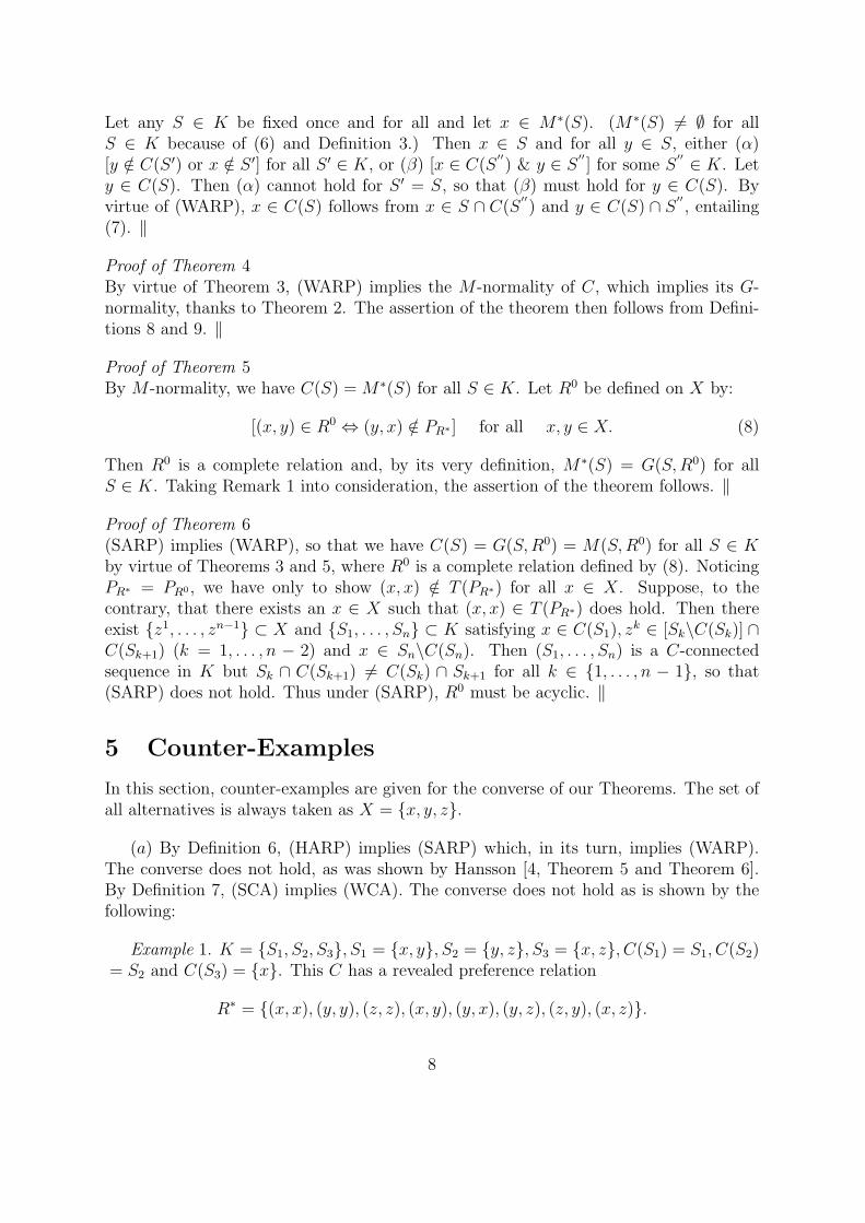
5 Counter-Examples
In this section, counter-examples are given for the converse of our Theorems. The set ofall alternatives is always taken as X = x, y, z.
(a) By Definition 6, (HARP) implies (SARP) which, in its turn, implies (WARP).The converse does not hold, as was shown by Hansson [4, Theorem 5 and Theorem 6].By Definition 7, (SCA) implies (WCA). The converse does not hold as is shown by thefollowing:
Example 1. K = S1, S2, S3, S1 = x, y, S2 = y, z, S3 = x, z, C(S1) = S1, C(S2)= S2 and C(S3) = x. This C has a revealed preference relation
R∗ = (x, x), (y, y), (z, z), (x, y), (y, x), (y, z), (z, y), (x, z).
8

(SCA) is not satisfied, because (z, x) ∈ T (R∗), x ∈ C(S3), z ∈ S3 but z /∈ C(S3). On theother hand, (WCA) is easily seen to be satisfied. ‖
(b) The converse of Theorem 2 does not hold in general; that is to say, there exists aG-normal choice function which is not M -normal.
Example 2. K = S1, S2, S1 = X,S2 = x, z, C(S1) = z, and C(S2) = x, z.In this case, R∗ = (z, z), (z, x), (z, y), (x, z), (x, x), so that we have G∗(S1) = z andG∗(S2) = x, z. Thus C is G-normal. But M∗(S1) = x, z 6= C(S1), so that C is notM -normal. ‖
(c) The converse of Theorem 3 does not hold in general. An example of a choicefunction which is M -rational but does not satisfy (WARP) will do.
Example 3. K = S1, S2, S1 = X,S2 = y, z, C(S1) = x, y and C(S2) = S2. Forthis C, R∗ = (x, x), (y, y), (z, z), (x, y), (x, z), (y, x), (y, z), (z, y). This C is M -normalas can be verified. (WARP) is, however, not satisfied, because S1 ∩ C(S2) = y, z andC(S1) ∩ S2 = y. ‖
(d) The converse of Theorem 4 is not true in general, as is shown by the followingexample.
Example 4. K = S1, S2, S1 = X,S2 = x, y, C(S1) = x and C(S2) = S2.Corresponding to this C, we have R∗ = (x, x), (y, y), (x, y), (x, z), (y, x). Therefore,M∗(S1) = x, y 6= C(S1). This C is not M -normal, hence (WARP) does not hold,thanks to Theorem 3. But we have C(S) = G(S,R1) = M(S,R2) for all S ∈ K, whereR1 = (x, x), (y, y), (x, y), (y, x), (x, z) and R2 = (z, y), (x, z). ‖
(e) The converse of Theorem 5 is falsified by the following example.
Example 5. K = S1, S2, S3, S1 = X,S2 = x, y, S3 = y, z, C(S1) = y, C(S2) =S2 and C(S3) = y. For this C, R∗ = (x, x), (y, y), (x, y), (y, x), (y, z). This C is notM -normal, because M∗(S1) = x, y 6= C(S1). But
R = (x, y), (y, x), (y, z), (z, x), (x, x), (y, y), (z, z)has the property C(S) = G(S,R) for all S ∈ K and R is complete, so that C is completerational. ‖
(f) The converse of Theorem 6 is falsified by the following example.
Example 6. K = S1, S2, S3, S1 = x, y, S2 = y, z, S3 = x, z, C(S1) = x, C(S2)= y and C(S3) = S3. As can be verified,
R = (x, x), (y, y), (z, z), (x, y), (y, z), (z, x), (x, z)
9

is an acyclic and complete relation such that C(S) = G(S, R) for all S ∈ K. (SARP)is, however, not satisfied, because S1 ∩ C(S2) = y, S2 ∩ C(S3) = z, S3 ∩ C(S1) =x, C(S1) ∩ S2 = ∅ and C(S2) ∩ S3 = ∅. ‖
(g) (WARP) is not strong enough to assure the acyclic and complete rationality ofthe choice function.
Example 7. K = S1, S2, S3, S1 = x, y, S2 = y, z, S3 = x, z, C(S1) = x, C(S2)= y and C(S3) = z. In this case, R∗ = (x, y), (y, z), (z, x). We are going to showthat R∗ ⊂ R∗. We have (x, y) ∈ R∗, because x ∈ C(S1), x /∈ S2 and y /∈ C(S3). Simi-larly z /∈ C(S1), y ∈ C(S2) and y /∈ S3 entail (y, z) ∈ R∗, while z /∈ S1, x /∈ C(S2) andz ∈ C(S3) show (z, x) ∈ R∗. Thus, thanks to Theorem 1 (i), this choice function satisfies(WARP). The unique complete rationalization thereof is, however, a cyclic one
R∗ = (x, y), (y, z), (z, x). ‖
6 Concluding Remarks
In conclusion, let us compare our results with Arrow-Sen theory, on the one hand, andthe Richter-Hansson theory, on the other. We are concerned with a choice function Con the family K. The choice mechanism C is said to be G-rational (resp. M -rational) ifthere exists a preference relation R such that the choice set C(S) can be identified withthe set of all R-greatest points (resp. R-maximal points) in S for any possible choicesituation S ∈ K. Note here that the concepts of G-rationality and M -rationality havenothing to do with the transitivity of the rationalization R. If R happens to satisfy theordering axiom of completeness and transitivity, C is said to be regular-rational. Arrow[1] and Sen [13] showed that:
(α) (SCA),(WCA),(SARP) and (WARP) are mutually equivalent necessary and suffi-cient conditions for regular-rationality if K includes all the pairs and all the triples takenfrom the basic set X .
It seems to us that the cost paid for the neat result (α) is rather high. Their as-sumption on the content of K might not generally be admissible, hence depriving theirresult of its general applicability. On the other hand, Richter [9] and Hansson [4] madevirtually no restrictions on the content of K and established that:
(β) (SCA) and (HARP) are mutually equivalent necessary and sufficient conditionsfor regular-rationality .
Later, Richter [10] extended his conceptual framework and established the followingcharacterization of G-rational choice functions.
(γ) G-normality is a necessary and sufficient condition for G-rationality .
10

[Insert Figure 1 around here.]
In this paper, we have systematically examined the structure of G-rational and M -rational choice functions. The domain of the choice function is assumed simply to bea non-empty family of non-empty sets. Thus we may reasonably claim the general ap-plicability of our results. The role of (SARP), (WARP), (WCA) and M -normality areclarified in this general setting.
Our results, together with (β) and (γ), are summarized in Figure 1. An arrow indi-cates implication, and cannot in general be reversed. The contrast with the Arrow-Senresult (α) is clear.
7 Appendix
(a) The Equivalence between (1) and (WARP)[(WARP) ⇒ (1)] Let us assume that (x, y) ∈ R∗∗ and (y, x) ∈ R∗ for some x and y inX. Then there exist S1 and S2 in K such that x ∈ C(S1), y ∈ S1\C(S1), x ∈ S2 andy ∈ C(S2). It follows that (S1, S2) is a C-connected pair in K but y /∈ C(S1) ∩ S2 andy ∈ S1 ∩ C(S2) so that (WARP) does not hold.
[(1)⇒ (WARP)] Let (S1, S2) be a C-connected pair in K such that x ∈ S1∩C(S2) andx /∈ C(S1)∩S2 for some x in X. Then (y, x) ∈ R∗∗ and (x, y) ∈ R∗ for any y ∈ C(S1)∩S2,negating (1).
(b)The Equivalence between (2) and (SARP)[(SARP) ⇒ (2)] Suppose that (x, y) ∈ T (R∗∗) and (y, x) ∈ R∗ for some x and y in X.Then either (x, y) ∈ R∗∗ or (x, z1),(z1, z2), . . . , (zn, y) ∈ R∗∗ for some z1, . . . , zn ∈ X.In view of (a) and Definition 6, we have only to consider the latter case. In this case,there exist S1, . . . , Sn and S in K such that x ∈ C(S1), z1 ∈ S1\C(S1), z1 ∈ C(S2),z2 ∈ S2\C(S2), . . ., zn ∈ C(Sn+1), y ∈ Sn+1\C(Sn+1), y ∈ C(S) and x ∈ S. Then(S1, . . . , Sn+1, S) is a C-connected sequence in K. But
z1 ∈ [S1 ∩ C(S2)]\[C(S1) ∩ S2], z2 ∈ [S2 ∩ C(S3)]\[C(S2) ∩ S3], . . . ,
y ∈ [Sn+1 ∩C(S)]\[C(Sn+1)∩S],
so that (SARP) does not hold.
[(2)⇒(SARP)] Let (S1, . . . , Sn) be any C-connected sequence in K. If
Sn−1 ∩ C(Sn) = C(Sn−1) ∩ Sn,
there remains nothing to be proved. Suppose, then, that Sn−1 ∩ C(Sn) 6= C(Sn−1) ∩ Sn.Firstly, suppose that there exists an x ∈ X such that x ∈ C(Sn−1)∩C(Sn) and x /∈ Sn−1∩C(Sn). In this case, for any y ∈ Sn−1 ∩ C(Sn), we have (x, y) ∈ R∗ and (y, x) ∈ R∗∗ incontradiction to (2). Secondly, suppose that we have x /∈ C(Sn−1)∩Sn, x ∈ Sn−1∩C(Sn)and y ∈ C(Sn−1) ∩ Sn for some x and y in X. Here again we have (x, y) ∈ R∗ and
11

(y, x) ∈ R∗∗ in contradiction to (2). Finally, suppose that C(Sn−1)∩Sn = ∅. (S1, . . . , Sn)being a C-connected sequence in K, x ∈ Sn−1 ∩C(Sn) for some x in X. If x ∈ C(Sn−1),we have x ∈ C(Sn−1) ∩ C(Sn) ⊂ C(Sn−1) ∩ Sn, a contradiction. Thus we obtain x ∈Sn−1\C(Sn−1). If Sn−2∩C(Sn−1) = C(Sn−2)∩Sn−1, there remains nothing to be proved.Otherwise, we repeat the above procedure to obtain a zn−1 ∈ [Sn−2\C(Sn−2)]∩C(Sn−1).This algorithm leads us either to
Sk∩C(Sk+1) = C(Sk)∩Sk+1 for some k ∈ 1, . . . , n−1 . . . (1∗)
or to:There exist z2, . . . , zn−1 such that z2 ∈ [S1\C(S1)] ∩ C(S2),
z3 ∈ [S2\C(S2)] ∩ C(S3), . . . , zn−1 ∈ [Sn−2\C(Sn−2)] ∩ C(Sn−1) . . . (2∗)
In the latter case, take a z1 ∈ C(S1) ∩ Sn. Then we obtain (z1, x) ∈ T (R∗∗) and(x, z1) ∈ R∗, in contradiction to (2). ‖
12
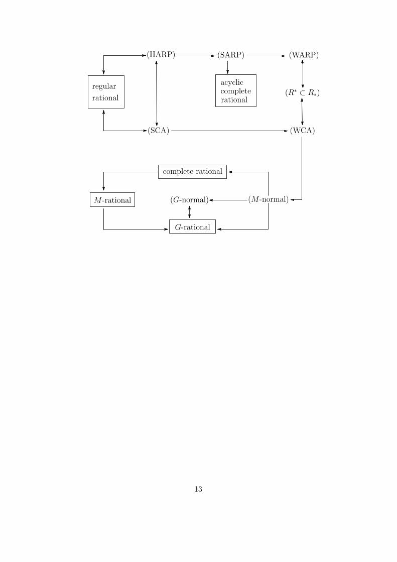
(HARP) (SARP) (WARP)
acycliccompleterational
regular
rational(R∗ ⊂ R∗)
(SCA) (WCA)
(M -normal)(G-normal)
G-rational
M -rational
complete rational
13

References
[1] Arrow, K. J., “Rational Choice Functions and Orderings,” Economica NS 26, 1959,121-127.
[2] Arrow, K. J., Social Choice and Individual Values, 2nd ed., New York: John Wiley& Sons, 1963.
[3] Fishburn, P. C., The Theory of Social Choice, New Jersey: Princeton UniversityPress, 1973.
[4] Hansson, B., “Choice Structures and Preference Relations,” Synthese 18, 1968, 443-458.
[5] Herzberger, H. G., “Ordinal Preference and Rational Choice,” Econometrica 41,1973, 187-237.
[6] Houthakker, H. S., “Revealed Preference and the Utility Function,” Economica NS17, 1950, 159-174.
[7] Jamison, D. T. and L. J. Lau, “Semiorders and the Theory of Choice,” Econometrica41, 1973, 901-912.
[8] Plott, C. R., “Path Independence, Rationality and Social Choice,” Econometrica41, 1973, 1075-1091.
[9] Richter, M. K., “Revealed Preference Theory,” Econometrica 34, 1966, 635-645.
[10] Richter, M. K., “Rational Choice,” in J. S. Chipman et al., eds., Preferences, Utility,and Demand, New York: Harcourt Brace Jovanovich, 1971, 29-58.
[11] Sen, A. K., “Quasi-Transitivity, Rational Choice and Collective Decisions,” Reviewof Economic Studies 36, 1969, 381-393.
[12] Sen, A. K., Collective Choice and Social Welfare, San Francisco: Holden-Day, 1970.
[13] Sen, A. K., “Choice Functions and Revealed Preference,” Review of Economic Stud-ies 38, 1971, 307-317.
[14] Samuelson, P. A., Foundations of Economic Analysis, Cambridge: Harvard Univer-sity Press, 1947.
[15] Suzumura, K., “General Possibility Theorems for Path-Independent Social Choice,”Kyoto Institute of Economic Research, Kyoto University, Discussion Paper 77, 1974.
[16] Wilson, R. B., “The Finer Structure of Revealed Preference,” Journal of EconomicTheory 2, 1970, 348-353.
14

Chapter 2Houthakker’s Axiom in the Theory of
Rational Choice∗
1 Introduction
In his celebrated classic paper [4], Houthakker strengthened Samuelson’s weak axiomof revealed preference [7, 8] into what he called semitransitivity , and showed that theLipschitz-continuous demand function of a competitive consumer satisfying his axiomdoes possess a generating utility function.1 Uzawa [11], Arrow [1], and others extendedthe conceptual framework of revealed preference theory so as to make it applicable toa wider class of problems. Instead of confining our attention to a demand function ofa competitive consumer, we are now concerned with a choice function over a familyof nonempty subsets of a basic nonempty set. A natural question suggests itself: Whatproperty of a choice function guarantees the existence of a generating preference ordering(GPO)? In particular, does Houthakker’s axiom, if suitably reformulated, qualify assuch? It is this problem of the existence of a GPO that constitutes the problem ofrationalizability of a choice function, which is a choice-functional counterpart of theintegrability problem in demand theory.
In the literature we have two answers to this question, depending on the extent ofthe domain of a choice function. On the one hand, if the family over which a choicefunction is defined contains all finite subsets of the whole space, the weak axiom ensuresthe existence of a GPO and that the strong axiom of revealed preference (which was sonamed by Samuelson [8] and attributed to Houthakker) is equivalent to the weak axiom[1, 9]. On the other hand, if we do not impose any such additional assumption on thedomain, the strong axiom is necessary but not sufficient for the existence of a GPO[3, 10].2 Richter [5] and Hansson [3] proposed in this general setting a necessary and
∗First published in Journal of Economic Theory, Vol.14, 1977, pp.284-290. Thanks are due to Pro-fessors W. M. Gorman and A. K. Sen for their comments. However, they should not be held responsiblefor any defects remaining in this chapter.
1Further results on this problem are found in papers collected in [2]. See, especially, Uzawa [2, Chap.1] and Hurwicz-Richter [2, Chap. 3].
2This statement is true for one version of the strong axiom, which is used by Arrow [1], Hansson [3],Sen [9] and Suzumura [10]. More about this in the final section.
15

sufficient condition for the existence of a GPO, which was called the congruence axiomby Richter.
The purpose of this paper is to show that Houthakker’s semitransitivity axiom, if suit-ably formalized in the choice-functional context, is in fact necessary and sufficient for theexistence of a GPO. Therefore it follows that, contrary to the prevailing interpretation,the strong axiom is not a legitimate formalization of Houthakker’s axiom which is equiv-alent to the congruence axiom. In other words, Houthakker’s axiom, unlike the strongaxiom, provides us with the precise restriction on a choice function for the rationalizabil-ity thereof, just as it provided us with the precise restriction on a Lipschitz-continuousdemand function for the integrability thereof.
2 Rationalizability
2.1. Let X be a nonempty set which stands for a fixed universe of alternatives. Weassume that there is a well-specified family K of nonempty subsets of X. The pair(X,K) will be called a choice space. A choice function on a choice space (X,K) is afunction C defined on K which assigns a non-empty subset (choice set) C(S) of S toeach S ∈ K.
A preference relation R on X is a binary relation on X, namely a subset of a Cartesianproduct X × X. Associated with a given preference relation R, an infinite sequence ofbinary relations R(τ)∞τ=1 is defined by R(1) = R, R(τ) = (x, y) ∈ X × X|(x, z) ∈R(τ−1) & (z, y) ∈ R for some z ∈ X(τ ≥ 2). The transitive closure of R is then definedby T (R) = ∪∞τ=1R
(τ).3 The strict preference relation PR corresponding to a preferencerelation R is an asymmetric component of R:
PR = (x, y) ∈ X ×X|(x, y) ∈ R & (y, x) /∈ R. (1)
We say that a preference relation R is transitive if (x, y) ∈ R and (y, z) ∈ R imply(x, z) ∈ R, acyclic if (x, x) /∈ T (PR), and complete if either (x, y) ∈ R or (y, x) ∈ R forall x and y in X. R is said to be an ordering if it is transitive and complete. For everyS ∈ K, we define
G(S, R) = x ∈ X|x ∈ S & (x, y) ∈ R for all y ∈ S, (2)
which is the set of all R-greatest points in S.
2.2. A preference relation R on X is said to rationalize a choice function C on (X, K)if we have
C(S) = G(S, R) for every S ∈ K. (3)
A choice function C is said to be rational if there exists a preference relation R whichrationalizes C. (R is then called a rationalization of C.) If a choice function C is rational
3It is easy to see that T satisfies the axiom of closure operations: (α) R ⊂ T (R) for every R, (β)R ⊂ R′ implies T (R) ⊂ T (R′) for every R and R′, (γ) T [T (R)] = T (R) for every R, and (δ) T (∅) = ∅.
16
with an acyclic rationalization, we say that C is acyclic rational . Similarly, if C is rationalwith an ordering rationalization, we say that C is full rational .
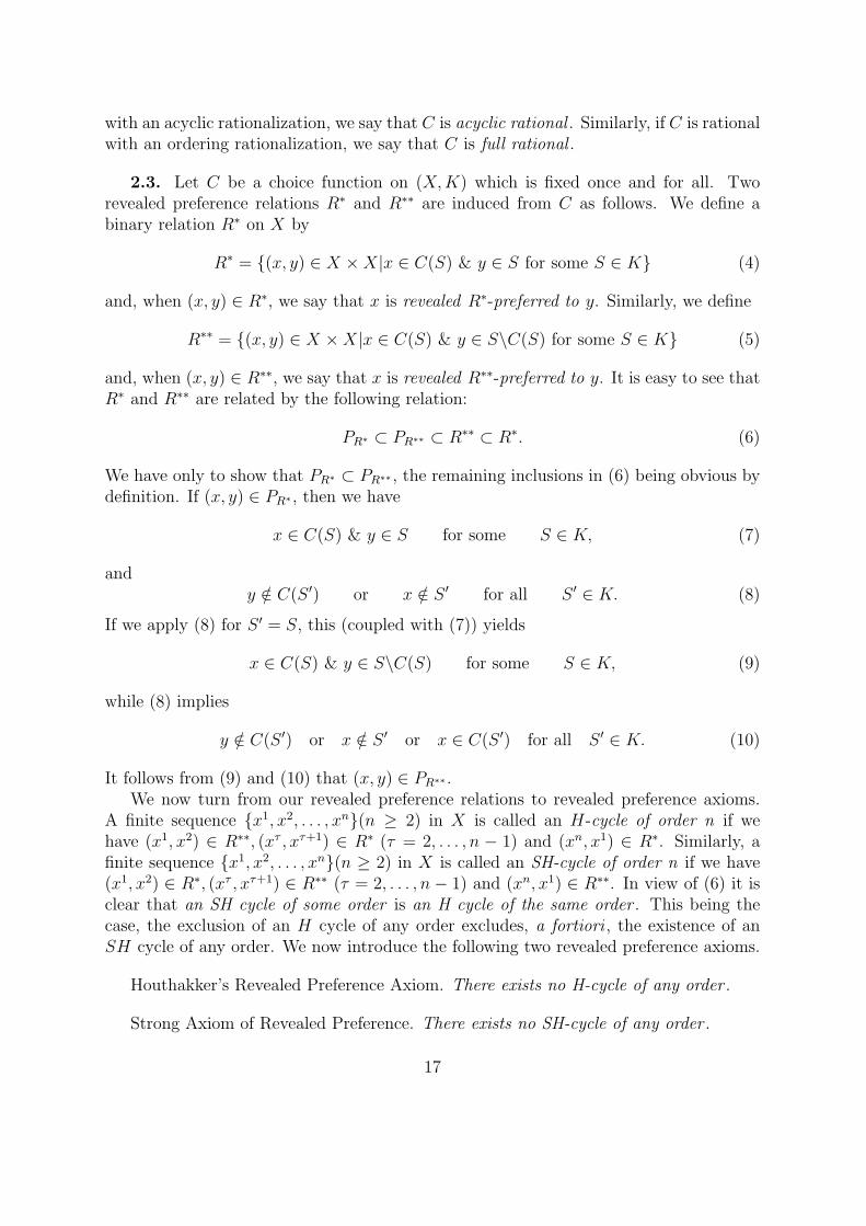
2.3. Let C be a choice function on (X,K) which is fixed once and for all. Tworevealed preference relations R∗ and R∗∗ are induced from C as follows. We define abinary relation R∗ on X by
R∗ = (x, y) ∈ X ×X|x ∈ C(S) & y ∈ S for some S ∈ K (4)
and, when (x, y) ∈ R∗, we say that x is revealed R∗-preferred to y. Similarly, we define
R∗∗ = (x, y) ∈ X ×X|x ∈ C(S) & y ∈ S\C(S) for some S ∈ K (5)
and, when (x, y) ∈ R∗∗, we say that x is revealed R∗∗-preferred to y. It is easy to see thatR∗ and R∗∗ are related by the following relation:
PR∗ ⊂ PR∗∗ ⊂ R∗∗ ⊂ R∗. (6)
We have only to show that PR∗ ⊂ PR∗∗ , the remaining inclusions in (6) being obvious bydefinition. If (x, y) ∈ PR∗ , then we have
x ∈ C(S) & y ∈ S for some S ∈ K, (7)
andy /∈ C(S ′) or x /∈ S ′ for all S ′ ∈ K. (8)
If we apply (8) for S ′ = S, this (coupled with (7)) yields
x ∈ C(S) & y ∈ S\C(S) for some S ∈ K, (9)
while (8) implies
y /∈ C(S ′) or x /∈ S ′ or x ∈ C(S ′) for all S ′ ∈ K. (10)
It follows from (9) and (10) that (x, y) ∈ PR∗∗ .We now turn from our revealed preference relations to revealed preference axioms.
A finite sequence x1, x2, . . . , xn(n ≥ 2) in X is called an H-cycle of order n if wehave (x1, x2) ∈ R∗∗, (xτ , xτ+1) ∈ R∗ (τ = 2, . . . , n − 1) and (xn, x1) ∈ R∗. Similarly, afinite sequence x1, x2, . . . , xn(n ≥ 2) in X is called an SH-cycle of order n if we have(x1, x2) ∈ R∗, (xτ , xτ+1) ∈ R∗∗ (τ = 2, . . . , n− 1) and (xn, x1) ∈ R∗∗. In view of (6) it isclear that an SH cycle of some order is an H cycle of the same order . This being thecase, the exclusion of an H cycle of any order excludes, a fortiori , the existence of anSH cycle of any order. We now introduce the following two revealed preference axioms.
Houthakker’s Revealed Preference Axiom. There exists no H-cycle of any order .
Strong Axiom of Revealed Preference. There exists no SH-cycle of any order .
17

Clearly, Houthakker’s axiom is stronger than the strong axiom. We have shown in [10]that the strong axiom is necessary but not sufficient for full rationality and that it issufficient but not necessary for acyclic rationality. In the final section we will arguethat the above-stated Houthakker’s axiom is a proper choice-functional counterpart ofHouthakker’s semitransitivity in demand theory.
2.4. We are now ready to put forward our theorem.
Rationalizability Theorem. A choice function C is full rational if and only if it satisfiesHouthakker’s axiom of revealed preference.
Proof of Necessity . If C is full rational with an ordering rationalization R, thenwe have (3). Suppose that there exists a sequence x1, x2, . . . , xn(n ≥ 2) such that(x1, x2) ∈ R∗∗ and (xτ , xτ+1) ∈ R∗ (τ = 1, 2, . . . , n − 1). Then there exists a sequenceS1, S2, . . . , Sn−1 in K such that x1 ∈ C(S1), x2 ∈ S1\C(S1), xτ ∈ C(Sτ ), and xτ+1 ∈Sτ (τ = 2, . . . , n−1). Since C is full rational we then have (x1, x2) ∈ PR and (xτ , xτ+1) ∈R (τ = 2, . . . , n − 1), which entails (x1, xn) ∈ PR, thanks to the transitivity of R. Butthis result excludes the possibility that (xn, x1) ∈ R∗, so that there exist no H-cylcle ofany order.
Proof of Sufficiency . Let a diagonal ∆ be defined by
∆ = (x, x) ∈ X ×X|x ∈ X, (11)
and define a binary relation Q by
Q = ∆ ∪ T (R∗). (12)
It is easy to see that Q is transitive and reflexive: (x, x) ∈ Q for all x in X. Thanks to acorollary of Szpilrajn’s theorem [3, Lemma 3] there exists an ordering R which subsumesQ; namely, there exists an ordering R such that
Q ⊂ R, (13)
andPQ ⊂ PR. (14)
We are going to show that this R in fact satisfies
R∗ ⊂ R, (15)
andPR∗ ⊂ PR. (16)
The former is obvious in view of R∗ ⊂ T (R∗), (12), and (13). To prove the latter wehave only to show that PR∗ ⊂ PQ, thanks to (14). Assume (x, y) ∈ PR∗ , which means(x, y) ∈ R∗ and (y, x) /∈ R∗. From (x, y) ∈ R∗ it follows that (x, y) ∈ Q. It only remains
18

to be shown that (y, x) /∈ Q. Assume, therefore, that (y, x) ∈ Q. Clearly, (y, x) /∈ ∆, elsewe cannot have (x, y) ∈ PR∗ . It follows that (y, x) ∈ T (R∗), which, in combination with(x, y) ∈ PR∗ ⊂ R∗∗, implies the existence of an H-cycle of some order, a contradiction.Therefore (15) and (16) are valid.
Let an S ∈ K be chosen and let x ∈ C(S). Then (x, y) ∈ R∗ for all y ∈ S. In viewof (15) we then have x ∈ G(S, R). It follows that
C(S) ⊂ G(S,R). (17)
Next let x ∈ S\C(S) and take y ∈ C(S), so that (y, x) ∈ R∗∗. If we have (x, y) ∈ R∗
it turns out that x, y is an H-cycle of order 2, a contradiction. Therefore we must have(x, y) /∈ R∗, which, in view of (y, x) ∈ R∗∗ ⊂ R∗, implies (y, x) ∈ PR∗ . Thanks to (16) wethen have (y, x) ∈ PR, entailing x ∈ S\G(S, R). Therefore we obtain
G(S, R) ⊂ C(S). (18)
As (17) and (18) are valid for any S ∈ K we have shown that C is full rational with anordering rationalization R. This completes the proof.
3 Comments on the Literature
It only remains to make some comments on the existing literature.(i) Houthakker [4, pp.162-163] introduced his semitransitivity axiom in terms of a
demand function h on the family of competitive budgets. Let Ω, p, and m be the com-modity space, a competitive price vector, and an income. Then h is a function on thefamily of all budget sets
B(p,m) = x ∈ Ω|px ≤ m. (19)
We consider a sequence xτTτ=1 in Ω satisfying
xτ = h(pτ , pτxτ ) for every τ ∈ 1, 2, . . . , T, (20)
xτ+1 ∈ B(pτ , pτxτ ) for every τ ∈ 1, 2, . . . , T − 1, (21)
andxτ+1 6= h(pτ , pτxτ ) for at least one τ ∈ 1, 2, . . . , T − 1. (22)
Houthakker’s semitransitivity then requires that x1 /∈ B(pT , pT xT ). It will be noticedthat what we called Houthakker’s axiom of revealed preference in Section 2.3 is a naturalreformulation of this requirement in terms of a choice function C.
(ii) What Samuelson [8, pp. 370-371] called the strong axiom is the same requirementas Houthakker’s, save for the replacement of (22) by
xτ+1 6= h(pτ , pτxτ ) for every τ ∈ 1, 2, . . . , T − 1. (23)
Our strong axiom of revealed preference in Section 2.3 is, it will be noticed, a naturalextension of Samuelson’s axiom in the context of a choice function.
19

(iii) We have shown in [10] that Hansson’s strong axiom of revealed preference [3] is,despite its apparent difference, equivalent to that of ours in Section 2.3.
(iv) Richter [5, p.637] argued that “the revealed preference notions employed in [theWeak Axiom of Samuelson and the Strong Axiom of Houthakker] are relevant only tothe special case of competitive consumers, so that axioms also have meaning only in thatlimited context.” However, these axioms can be and have been generalized beyond thenarrow confinement of competitive consumers. Besides, Richter himself defined in [6]the weak and the strong axioms for a single-valued choice function. There is no reason,furthermore, that we should not consider these axioms in terms of a set-valued choicefunction.
In conclusion, it is hoped that our result will help to clarify the central role playedby Houthakker’s axiom in the whole spectrum of revealed preference theory.
20

References
[1] Arrow, K. J., “Rational Choice Functions and Orderings,” Economica NS 26, 1959,121-127.
[2] Chipman, J. S., L. Hurwicz, M. K. Richter and H. F. Sonnenschein, eds., Preferences,Utility, and Demand , Harcourt Brace Jovanovich, New York, 1971.
[3] Hansson, B., “Choice Structures and Preference Relations,” Synthese 18, 1968, 443-458.
[4] Houthakker, H. S., “Revealed Preference and the Utility Function,” Economica NS17, 1950, 159-174.
[5] Richter, M. K., “Revealed Preference Theory,” Econometrica 34, 1966, 635-645.
[6] Richter, M. K., “Rational Choice,” in J. S. Chipman et al., eds., Preferences, Utility,and Demand, New York: Harcourt Brace Jovanovich, 1971, 29-58.
[7] Samuelson, P. A., “A Note on the Pure Theory of Consumer’s Behaviour,” Econom-ica NS 5, 1938, 61-71, 353-354.
[8] Samuelson, P. A., “The Problem of Integrability in Utility Theory,” Economica NS17, 1950, 355-385.
[9] Sen, A. K., “Choice Functions and Revealed Preference,” Review of Economic Stud-ies 38, 1971, 307-317.
[10] Suzumura, K., “Rational Choice and Revealed Preference,” Review of EconomicStudies 43, 1976, 149-158. Chapter 1 of this volume.
[11] Uzawa, H., “Note on Preference and Axioms of Choice,” Annals of the Institute ofStatistical Mathematics 8, 1957, 35-40.
21

Chapter 3Consistent Rationalizability∗
1 Introduction
Rationalizability is an important issue in the analysis of economic decisions. It provides ameans to test theories of choice, including — but not limited to — traditional consumerdemand theory. The central question to be addressed is as follows: are the observedchoices of an economic agent compatible with our standard theories of choice as beingmotivated by optimizing behaviour? More precisely, can we find a preference relationwith suitably defined properties that generates the observed choices as the choice ofgreatest or maximal elements according to this relation? This question has its origin inthe theory of consumer demand but has since been explored in more general contexts,including both individual and collective choice. By formulating necessary and sufficientconditions for the existence of a rationalizing relation, testable restrictions on observablechoice behaviour implied by the various theories are established.
Samuelson [12] began his seminal paper on revealed preference theory with a remarkthat “[f]rom its very beginning the theory of consumer’s choice has marched steadilytowards greater generality, sloughing off at successive stages unnecessarily restrictiveconditions” (Samuelson [12, p.61]). Even after Samuelson [12; 13, Chapter V; 14; 15] laidthe foundations of “the theory of consumer’s behaviour freed from any vestigial tracesof the utility concept” (Samuelson [12, p.71]), the exercise of Ockham’s Razor persistedwithin revealed preference theory. Capitalizing on Georgescu-Roegen’s [5, p.125; 15,p.222] observation that the intuitive justification of the axioms of revealed preferencetheory has nothing to do with the special form of budget sets, but instead, is basedon the implicit consideration of choices from two-element sets. Arrow [2] expanded theanalysis of rational choice and revealed preference beyond consumer choice problems.He pointed out that “the demand-function point of view would be greatly simplified ifthe range over which the choice functions are considered to be determined is broadened
∗First published in Economica, Vol.72, 2005, pp.185-200. Joint paper with W. Bossert and Y. Spru-mont. Financial support through grants from the Social Sciences and Humanities Research Council ofCanada, the Fonds pour la Formation de Chercheurs et l’Aide a la Recherche of Quebec, and a Grant-in-Aid for Scientific Research for Priority Areas Number 603 from the Ministry of Education, Culture,Sports, Science and Technology of Japan is gratefully acknowledged. The paper was presented at BocconiUniversity. We thank three referees assigned by Economica for comments and suggestions.
22
to include all finite sets” (Arrow, [2, p.122]). Sen [16, p.312] defended Arrow’s domainassumption by posing two important questions: “why assume the axioms [of revealedpreference] to be true only for ‘budget sets’ and not for others?” and “[a]re there reasonsto expect that some of the rationality axioms will tend to be satisfied in choices over‘budget sets’ but not for other choices?”
While it is certainly desirable to liberate revealed preference theory from the narrowconfinement of budget sets, the admission of all finite subsets of the universal sets intothe domain of a choice function may well be unsuitable for many applications. In thiscontext, two important groups of contributions stand out. In the first place, Richter [10;11], Hansson [7] and Suzumura [17; 19; 20, Chapter 2] developed the theory of rationalchoice and revealed preference for choice functions with general non-empty domains whichdo not impose any extraneous restrictions whatsoever on the class of feasible sets. In thesecond place, Sen [16] showed that Arrow’s results (as well as others with similar features)do not hinge on the full power of the assumption that all finite sets are included in thedomain of a choice function — it suffices if the domain contains all two-element andthree-element sets.
It was in view of this current state of the art that Bossert, Sprumont and Suzumura[3] examined two crucial types of general domain in an analysis of several open questionsin the theory of rational choice. The first is the general domain a la Richter, Hanssonand Suzumura, and the second is the class of base domains which include all singletonsand all two-element subsets of the universal set. The status of the general domain seemsto be impeccable, as the theory developed on this domain is relevant in whatever choicesituations we may care to specify. The base domains also seem to be on safe ground, as theconcept of rational choice as maximizing choice is intrinsically connected with pairwisecomparisons: singletons can be viewed as pairs with identical components, whereas two-element sets represent pairs of distinct alternatives. As Arrow [1, p.16] put it, “one of theconsequences of the assumptions of rational choice is that the choice in any environmentcan be determined by a knowledge of the choices in two-element environments.”
In this chapter, we focus on the rationalizability of choice functions by means ofconsistent relations. The concept of consistency was first introduced by Suzumura [18],and it is a weakening of transitivity requiring that any preference cycle should involveindifference only. As was shown by Suzumura [18; 20, Chapter 1], consistency is necessaryand sufficient for the existence of an ordering extension of a binary relation. For thatreason, consistency is a central property for the analysis of rational choice as well: in orderto obtain a rationalizing relation that is an ordering, an extension procedure is, in general,required in order to ensure that the rationalization is complete. Violations of transitivityare quite likely to be observed in practical choice situations. For instance, Luce’s [9]well-known coffee-sugar example provides a plausible argument against assuming thatindifference is always transitive: the inability of a decision-maker to perceive ‘small’differences in alternatives is bound to lead to intransitivities. As this example illustrates,transitivity frequently is too strong an assumption to impose in the context of individualchoice. In collective choice problems, it is even more evident that the plausibility oftransitivity can be questioned. On the other hand, it is difficult to interpret observed
23

choices as ‘rational’ if they do not possess any coherence property. Because of Suzumura’s[18] result, consistency can be considered a weakening of transitivity that is minimal inthe sense that it cannot be weakened further without abandoning all hope of finding arationalizing ordering extension.
To further underline the importance of consistency, note that this property is preciselywhat is required to prevent the problem of a ‘money pump.’ If consistency is violated,there exists a preference cycle with at least one strict preference. In this case, the agentunder consideration is willing to trade an alternative x0 for another alternative x1 (where‘willingness to trade’ is to be interpreted as being at least as well-off after the trade asbefore), x1 for an alternative x2 and so on until we reach an alternative xK such that theagent strictly prefers getting back x0 to retaining possession of xK . Thus, at the end ofa chain of exchanges, the agent is willing to pay a positive amount in order to get backthe alternative it had in its possession in the first place — a classical example of a moneypump.
We examine consistent rationalizability under two domain assumptions. The first is,again, the general domain assumption where no restrictions whatsoever are imposed, andthe second weakens the base domain hypothesis: we merely require the domain to containall two-element sets but not necessarily all singletons, and we refer to those domains asbinary domains. Thus, our results are applicable in a wide range of choice problems.Unlike many contributions to the theory of rational choice, we do not have to assumethat triples are part of the domain. Especially the first domain assumption — the generaldomain — is highly relevant because it can accommodate any choice situation that arisesin the analysis of both individual and collective choice. For instance, our results areapplicable in traditional demand theory but in more general environments as well.
Depending on the additional properties that can be imposed on rationalizations (re-flexivity and completeness), different notions of consistent rationalizability can be defined.We characterize all but one of those notions in the general case, and all of them in thecase of binary domains. It is worth noting that we obtain full characterization results onbinary domains (in particular, on domains that do not have to contain any triples), eventhough consistency imposes a restriction on possible cycles of any length.
In Section 2, the notation and our basic definitions are presented, along with somepreliminary lemmas. Section 3 develops the theory of consistent rationalizability on gen-eral domains, whereas Section 4 expounds the corresponding theory on binary domains.Some concluding remarks are collected in Section 5.
2 Preliminaries
The set of positive (resp. non-negative) integers is denoted by N (resp. N0). For a setS, |S| is the cardinality of S. Let X be a universal non-empty set of alternatives. X isthe power set of X excluding the empty set. A choice function is a mapping C : Σ → Xsuch that C(S) ⊆ S for all S ∈ Σ, where Σ ⊆ X with Σ 6= ∅ is the domain of C. Notethat C maps Σ into the set of all non-empty subsets of X. Thus, using Richter’s [11]terminology, the choice function C is assumed to be decisive. Let C(Σ) denote the image
24

of Σ under C, that is, C(Σ) = ∪S∈ΣC(S). In addition to arbitrary non-empty domains,to be called general domains, we consider binary domains which are domains Σ ⊆ Xsuch that S ∈ X | |S| = 2 ⊆ Σ.
Let R ⊆ X×X be a (binary) relation on X. The asymmetric factor P (R) of R is givenby (x, y) ∈ P (R) if and only if (x, y) ∈ R and (y, x) 6∈ R for all x, y ∈ X. The symmetricfactor I(R) of R is defined by (x, y) ∈ I(R) if and only if (x, y) ∈ R and (y, x) ∈ R for allx, y ∈ X. The non-comparable factor N(R) of R is given by (x, y) ∈ N(R) if and only if(x, y) 6∈ R and (y, x) 6∈ R for all x, y ∈ X.
A relation R ⊆ X ×X is (i) reflexive if, for all x ∈ X, (x, x) ∈ R; (ii) complete if, forall x, y ∈ X such that x 6= y, (x, y) ∈ R or (y, x) ∈ R; (iii) transitive if, for all x, y, z ∈ X,[(x, y) ∈ R and (y, z) ∈ R] implies (x, z) ∈ R; (iv) consistent if, for all K ∈ N \ 1 andfor all x0, . . . , xK ∈ X, (xk−1, xk) ∈ R for all k ∈ 1, . . . , K implies (xK , x0) 6∈ P (R); (v)P-acyclical if, for all K ∈ N \ 1 and for all x0, . . . , xK ∈ X, (xk−1, xk) ∈ P (R) for allk ∈ 1, . . . , K implies (xK , x0) 6∈ P (R).
The transitive closure of R ⊆ X × X is denoted by R, that is, for all x, y ∈ X,(x, y) ∈ R if there exist K ∈ N and x0, . . . , xK ∈ X such that x = x0, (xk−1, xk) ∈ R forall k ∈ 1, . . . , K and xK = y. Clearly, R is transitive and, because we can set K = 1,it follows that R ⊆ R. For future reference, we state the following well-known result theproof of which is straightforward and thus omitted (see Suzumura [20, pp.11–12]).
Lemma 1 Let R and Q be binary relations on X. If R ⊆ Q, then R ⊆ Q.
The direct revealed preference relation RC ⊆ X ×X of a choice function C with anarbitrary domain Σ is defined as follows. For all x, y ∈ X, (x, y) ∈ RC if there existsS ∈ Σ such that x ∈ C(S) and y ∈ S. The (indirect) revealed preference relation of C isthe transitive closure RC of the direct revealed preference relation RC .
For S ∈ Σ and a relation R ⊆ X ×X, the set of R-greatest elements in S is x ∈ S |(x, y) ∈ R for all y ∈ S, and the set of R-maximal elements in S is x ∈ S | (y, x) 6∈P (R) for all y ∈ S. A choice function C is greatest-element rationalizable if there existsa relation R on X, to be called a G-rationalization, such that C(S) is equal to the setof R-greatest elements in S for all S ∈ Σ. C is maximal-element rationalizable if thereexists a relation R on X, to be called an M-rationalization, such that C(S) is equal tothe set of R-maximal elements in S for all S ∈ Σ. We use the term rationalization ingeneral discussions where it is not specified whether greatest-element rationalizability ormaximal-element rationalizability is considered.
If a rationalization is required to be reflexive and complete, the notions of greatest-element rationalizability and that of maximal-element rationalizability coincide. Withoutthese properties, however, this is not necessarily the case. Greatest-element rationaliz-ability is based on the idea of chosen alternative weakly dominating all alternatives inthe feasible set under consideration, whereas maximal-element rationalizability requireschosen elements not to be strictly dominated by any other feasible alternative. Specificexamples illustrating the differences between those two concepts will be discussed later.
Depending on the properties that we might want to impose on a rationalization,different notions of rationalizability can be defined. For simplicity of presentation, we
25

use the following notation. G (resp. RG; CG; RCG) stands for greatest-element ra-tionalizability by means of a consistent (resp. reflexive and consistent; complete andconsistent; reflexive, complete and consistent) G-rationalization. Analogously, M (resp.RM; CM; RCM) is maximal-element rationalizability by means of a consistent (resp.reflexive and consistent; complete and consistent; reflexive, complete and consistent) M-rationalization. Note that we do not identify consistency explicitly in these acronymseven though it is assumed to be satisfied by the rationalization in question. This is be-cause consistency is required in all of the theorems presented in this paper, so that the useof another piece of notation would be redundant and likely increase the complexity of ourexposition. However, note that the two lemmas stated below do not require consistency.In particular, the implication of part (i) of Lemma 3 does not apply to rationalizabilityby a consistent relation; see also Theorem 1.
We conclude this section with two further preliminary results. We first present thefollowing lemma, the first part of which is due to Samuelson [12; 14]; see also Richter[11]. It states that the direct revealed preference relation must be contained in any G-rationalization and, moreover, that if an alternative x is directly revealed preferred to analternative y, then y cannot be strictly preferred to x by any M-rationalization.
Lemma 2 (i) If R is a G-rationalization of C, then RC ⊆ R.(ii) If R is an M-rationalization of C, then RC ⊆ R ∪N(R).
Proof. (i) Suppose that R is a G-rationalization of C and x, y ∈ X are such that(x, y) ∈ RC . By definition of RC , there exists S ∈ Σ such that x ∈ C(S) and y ∈ S.Because R is a G-rationalization of C, we obtain (x, y) ∈ R.
(ii) Suppose R is an M-rationalization of C and x, y ∈ X are such that (x, y) ∈ RC .By way of contradiction, suppose (x, y) 6∈ R ∪N(R). Therefore, (y, x) ∈ P (R). BecauseR maximal-element rationalizes C, this implies x 6∈ C(S) for all S ∈ Σ such that y ∈ S.But this contradicts the hypothesis (x, y) ∈ RC .
Our final preliminary observation concerns the relationship between maximal-elementrationalizability and greatest-element rationalizability when no further restrictions areimposed on a rationalization. This applies, in particular, when consistency is not im-posed. Moreover, an axiom that is necessary for either form of rationalizability is pre-sented. This requirement is referred to as the V-axiom in Richter [11]; we call it direct-revelation coherence in order to have a systematic terminology throughout this chapter.
Direct-Revelation Coherence: For all S ∈ Σ, for all x ∈ S, if (x, y) ∈ RC for ally ∈ S, then x ∈ C(S).
Suzumura [17] establishes that, in the absence of any requirements on a rationaliza-tion, maximal-element rationalizability implies greatest-element rationalizability. Fur-thermore, Richter [11] shows that direct-revelation coherence is necessary for greatest-element rationalizability by an arbitrary G-rationalization on an arbitrary domain. Wesummarize these observations in the following lemma. For completeness, we provide aproof.
26

Lemma 3 (i) If C is maximal-element rationalizable, then C is greatest-element ratio-nalizable.
(ii) If C is greatest-element rationalizable, then C satisfies direct-revelation coherence.
Proof. (i) Suppose R is an M-rationalization of C. It is straightforward to verify thatR′ = (x, y) | (y, x) 6∈ P (R) is a G-rationalization of C.
(ii) Suppose R is a G-rationalization of C, and let S ∈ Σ and x ∈ S be such that(x, y) ∈ RC for all y ∈ S. By part (i) of Lemma 2, (x, y) ∈ R for all y ∈ S. Because R isa G-rationalization of C, this implies x ∈ C(S).
There are alternative notions of rationality such as that of Kim and Richter [8] whoproposed the concept of motivated choice: C is a motivated choice if there exist a relationR on X, which is to be called a motivation of C, such that
C(S) = x ∈ S | (y, x) 6∈ R for all y ∈ S
for all S ∈ Σ. This property is implied by maximal-element rationalizability but theconverse implication is not true. Moreover, C is a motivated choice if and only if C isgreatest-element rationalizable. Indeed, R greatest-element rationalizes C if and only ifits dual Rd, which is defined by
(x, y) ∈ Rd ⇔ (y, x) 6∈ R
for all x, y ∈ X, is a motivation of C.Richter [11] shows that direct-revelation coherence is not only necessary but also suf-
ficient for greatest-element rationalizability on an arbitrary domain, without any furtherrestrictions imposed on the G-rationalization. Moreover, the axiom is necessary and suf-ficient for greatest-element rationalizability by a reflexive (but otherwise unrestricted)rationalization on an arbitrary domain. The requirement remains, of course, necessaryfor greatest-element rationalizability if we restrict attention to binary domains. As shownbelow, if we add consistency as a requirement on a rationalization, direct-revelation coher-ence by itself is sufficient for neither greatest-element rationalizability nor for maximal-element rationalizability, even on binary domains.
3 General Domains
In this section, we impose no restrictions on the domain Σ. We begin our analysis byproviding a full description of the logical relationships between the different notions ofrationalizability that can be defined, given our consistency assumption imposed on arationalization. The possible definitions of rationalizability that can be obtained dependon whether reflexivity or completeness are added to consistency. Furthermore, a distinc-tion between greatest-element rationalizability and maximal-element rationalizability ismade. For convenience, a diagrammatic representation is employed: all axioms that are
27

depicted within the same box are equivalent, and an arrow pointing from one box b toanother box b′ indicates that the axioms in b imply those in b′, and no further implicationsare true without additional assumptions regarding the domain of C.
Theorem 1 Suppose Σ is a general domain. Then
RCG, CG, RCM, CM
↓ ↓RG, G RM, M
Proof. We proceed as follows. In Step 1, we prove the equivalence of all axioms thatappear in the same box. In Step 2, we show that all implications depicted in the theoremstatement are valid. In Step 3, we provide examples demonstrating that no furtherimplications are true in general.
Step 1. For each of the three boxes, we show that all axioms listed in the box areequivalent.
1.a. We first prove the equivalence of the axioms in the top box.Clearly, RCG implies CG and RCM implies CM. Moreover, if a relation R is
reflexive and complete, it follows that the set of R-greatest elements in S is equal tothe set of R-maximal elements in S for any S ∈ Σ. Therefore, RCG and RCM areequivalent.
To see that CM implies RCM, suppose R is a consistent and complete M-rationalizationof C. Let
R′ = R ∪ (x, x) | x ∈ X.Clearly, R′ is reflexive. R′ is consistent and complete because R is. That R′ is anM-rationalization of C follows immediately from the observation that R is.
To complete Step 1.a of the proof, it is sufficient to show that CG implies RCG.Suppose R is a consistent and complete G-rationalization of C. Let
R′ = [R ∪∆ ∪ (y, x) | x 6∈ C(Σ) & y ∈ C(Σ)] \ (x, y) | x 6∈ C(Σ) & y ∈ C(Σ),
where ∆ = (x, x)|x ∈ X. Clearly, R′ is reflexive by definition.To show that R′ is complete, let x, y ∈ X be such that x 6= y and (x, y) 6∈ R′. By
definition of R′, this implies
(x, y) 6∈ R and [x 6∈ C(Σ) or y ∈ C(Σ)]
orx 6∈ C(Σ) and y ∈ C(Σ).
28

If the former applies, the completeness of R implies (y, x) ∈ R and, by definition of R′,we obtain (y, x) ∈ R′. If the latter is true, (y, x) ∈ R′ follows immediately from thedefinition of R′.
Next, we show that R′ is consistent. Let K ∈ N \ 1 and x0, . . . , xK ∈ X be suchthat (xk−1, xk) ∈ R′ for all k ∈ 1, . . . , K. Clearly, we can, without loss of generality,assume that xk−1 6= xk for all k ∈ 1, . . . , K. We distinguish two cases.
(i) x0 6∈ C(Σ). In this case, it follows that x1 6∈ C(Σ); otherwise we would have(x1, x0) ∈ P (R′) by definition of R′, contradicting our hypothesis. Successively applyingthis argument to all k ∈ 1, . . . , K, we obtain xk 6∈ C(Σ) for all k ∈ 1, . . . , K. Bydefinition of R′, this implies (xk−1, xk) ∈ R for all k ∈ 1, . . . , K. By the consistency ofR, we must have (xK , x0) 6∈ P (R). Because xK 6∈ C(Σ), this implies, according to thedefinition of R′, (xK , x0) 6∈ P (R′).
(ii) x0 ∈ C(Σ). If xK 6∈ C(Σ), (xK , x0) 6∈ P (R′) follows immediately from the definition ofR′. If xK ∈ C(Σ), it follows that xK−1 ∈ C(Σ); otherwise we would have (xK−1, xK) 6∈ R′
by definition of R′, contradicting our hypothesis. Successively applying this argumentto all k ∈ 1, . . . , K, we obtain xk ∈ C(Σ) for all k ∈ 1, . . . , K. By definition of R′,this implies (xk−1, xk) ∈ R for all k ∈ 1, . . . , K. By the consistency of R, we musthave (xK , x0) 6∈ P (R). Because x0 ∈ C(Σ), this implies, according to the definition ofR′, (xK , x0) 6∈ P (R′).
Finally, we show that R′ is a G-rationalization of C. Let S ∈ Σ and x ∈ S.Suppose first that (x, y) ∈ R′ for all y ∈ S. If |S| = 1, x ∈ C(S) follows immediately
because C(S) is non-empty. If |S| ≥ 2, we obtain x ∈ C(Σ). Because R is a G-rationalization of C, this implies (x, x) ∈ R. By definition of R′, (x, z) ∈ R for allz ∈ C(S). Therefore, (x, z) ∈ R for all z ∈ C(S)∪x. Suppose, by way of contradiction,that x 6∈ C(S). Because R is a G-rationalization of C, it follows that there existsy ∈ S \ (C(S)∪x) such that (x, y) 6∈ R. The completeness of R implies (y, x) ∈ P (R).Let z ∈ C(S). It follows that (z, y) ∈ R because R is a G-rationalization of C and, asestablished earlier, (x, z) ∈ R. This contradicts the consistency of R.
To prove the converse implication, suppose x ∈ C(S). Because R is a G-rationalizationof C, we have (x, y) ∈ R for all y ∈ S. In particular, this implies (x, x) ∈ R and, accordingto the definition of R′, we obtain (x, y) ∈ R′ for all y ∈ S.
1.b. The proof that RM and M are equivalent is analogous to the proof of theequivalence of RCM and CM in Step 1.a.
1.c. Clearly, RG implies G. Conversely, suppose R is a consistent G-rationalizationof C. Let
R′ = (R ∪∆) \ (x, y) | x 6∈ C(Σ) & x 6= y.Clearly, R′ is reflexive.Next, we prove that R′ is consistent. Let K ∈ N \ 1 and x0, . . . , xK ∈ X be such
that (xk−1, xk) ∈ R′ for all k ∈ 1, . . . , K. Again, we can assume that xk−1 6= xk for all
29

k ∈ 1, . . . , K. By definition of R′, x0 ∈ C(Σ). The rest of the proof follows as in part(ii) of the consistency of the relation R′ in Step 1.a.
It remains to be shown that R′ is a G-rationalization of C. Let S ∈ Σ and x ∈ S.First, suppose (x, y) ∈ R′ for all y ∈ S. By definition of R′, (x, y) ∈ R for all
y ∈ S \x. Analogously to the corresponding argument in Step 1.a, the assumption x 6∈C(S) implies the existence of y ∈ S \ (C(S)∪ x) such that (x, y) 6∈ R, a contradiction.
Finally, suppose x ∈ C(S). This implies (x, y) ∈ R for all y ∈ S because R is aG-rationalization of C. Furthermore, because C(S) ⊆ C(Σ), we have x ∈ C(Σ). Bydefinition of R′, this implies (x, y) ∈ R′ for all y ∈ S.
Step 2. The implications corresponding to the arrows in the theorem statement arestraightforward.
Step 3. Given Steps 1 and 2, to prove that no further implications are valid, it issufficient to provide examples showing that (a) M does not imply G; and (b) G does notimply M. Note that this independence of M and G in the presence of consistency doesnot contradict part (i) of Lemma 3—consistency is not required in the lemma.
3.a. M does not imply G.
Example 1 Let X = x, y, z and Σ = x, y, x, z, y, z. For future reference,note that Σ is a binary domain. Define the choice function C by letting C(x, y) =x, y, C(x, z) = x, z and C(y, z) = y. This choice function is maximal-elementrationalizable by the consistent (and reflexive) rationalization
R = (x, x), (y, y), (y, z), (z, z).
Suppose C is greatest-element rationalizable by a consistent rationalization R′. BecauseC(Σ) = X, greatest-element rationalizability implies that R′ is reflexive. Therefore,because y ∈ C(y, z) and z 6∈ C(y, z), we must have (y, z) ∈ R′ and (z, y) 6∈ R′.Therefore, (y, z) ∈ P (R′). Because R′ is a G-rationalization of C, z ∈ C(x, z) implies(z, x) ∈ R′ and x ∈ C(x, y) implies (x, y) ∈ R′. This yields a contradiction to theassumption that R′ is consistent.
3.b. To prove that G does not imply M, we employ an example due to Suzumura[17, pp.151–152].
Example 2 Let X = x, y, z and Σ = x, y, x, z, x, y, z, and define C(x, y) =x, y, C(x, z) = x, z and C(x, y, z) = x. This choice function is greatest-element rationalizable by the consistent (and reflexive) rationalization
R = (x, x), (x, y), (x, z), (y, x), (y, y), (z, x), (z, z).
Suppose R′ is an M-rationalization of C. Because z ∈ C(x, z), maximal-elementrationalizability implies (x, z) 6∈ P (R′) and, consequently, z 6∈ C(x, y, z) implies
30

(y, z) ∈ P (R′). Analogously, y ∈ C(x, y) implies, together with maximal-element ra-tionalizability, (x, y) 6∈ P (R′) and, consequently, y 6∈ C(x, y, z) implies (z, y) ∈ P (R′).But this contradicts the above observation that we must have (y, z) ∈ P (R′). Note thatconsistency (or any other property) of R′ is not invoked in the above argument. More-over, R is reflexive. Thus, RG does not even imply maximal-element rationalizability byan arbitrary rationalization.
We now provide characterizations of two of the three notions of rationalizability iden-tified in the above theorem. The first is a straightforward consequence of Richter’s [10]result and the observation that consistency is equivalent to transitivity in the presence ofreflexivity and completeness. Richter [10] shows that the congruence axiom is necessaryand sufficient for greatest-element rationalizability by a transitive, reflexive and completerationalization. Congruence is defined as follows.
Congruence: For all x, y ∈ X, for all S ∈ Σ, if (x, y) ∈ RC , y ∈ C(S) and x ∈ S, thenx ∈ C(S).
We obtain the following:
Theorem 2 C satisfies RCG if and only if C satisfies congruence.
Proof. As is straightforward to verify, a relation is consistent, reflexive and complete ifand only if it is transitive, reflexive and complete. The result now follows immediatelyfrom the equivalence of congruence and greatest-element rationalizability by a transitive,reflexive and complete rationalization established by Richter [10].
In order to characterize G (and, therefore, RG; see Theorem 1), we employ theconsistent closure of the direct revealed preference relation RC . The consistent closureof a relation R is analogous to the transitive closure: the idea is to add all pairs to therelation R that must be in a G-rationalizing relation due to the requirement that therationalization be consistent. Define the consistent closure R∗ of R by
R∗ = R ∪ (x, y) | (x, y) ∈ R & (y, x) ∈ R.Clearly, R ⊆ R∗. To illustrate the definition of the consistent closure and its relationshipto the transitive closure, consider the following examples.
Example 3 Let X = x, y, z and R = (x, x), (x, y), (y, y), (y, z), (z, x), (z, z). Weobtain R∗ = R = X ×X.
Example 4 Let X = x, y, z and R = (x, y), (y, z). We have R∗ = R and R =(x, y), (y, z), (x, z).In Example 3, the consistent closure coincides with the transitive closure, whereas in Ex-ample 3, the consistent closure is a strict subset of the transitive closure. More generally,R∗ is always a subset of R; see Lemma 4 below. Moreover, the lemma establishes animportant property of R∗: just as R is the smallest transitive relation containing R, R∗
is the smallest consistent relation containing R.
31

Lemma 4 Let R be a binary relation on X.(i) R∗ ⊆ R.(ii) R∗ is the smallest consistent relation containing R.
Proof. (i) Suppose that (x, y) ∈ R∗. By definition,
(x, y) ∈ R or [(x, y) ∈ R & (y, x) ∈ R].
If (x, y) ∈ R, (x, y) ∈ R follows because R ⊆ R. If [(x, y) ∈ R & (y, x) ∈ R], (x, y) ∈ Ris implied trivially.
(ii) We first prove that R∗ is consistent. Suppose K ∈ N \ 1 and x0, . . . , xK ∈ Xare such that (xk−1, xk) ∈ R∗ for all k ∈ 1, . . . , K. We show that (xK , x0) 6∈ P (R∗).By part (i) of the lemma, (xk−1, xk) ∈ R for all k ∈ 1, . . . , K, and the transitivity of Rimplies
(x0, xK) ∈ R. (1)
If (xK , x0) 6∈ R∗, we immediately obtain (xK , x0) 6∈ P (R∗) and we are done. Nowsuppose that (xK , x0) ∈ R∗. By definition of R∗, we must have
(xK , x0) ∈ R or [(xK , x0) ∈ R & (x0, xK) ∈ R].
If (xK , x0) ∈ R, (1) and the definition of R∗ together imply (x0, xK) ∈ R∗ and, thus,(xK , x0) 6∈ P (R∗). If (xK , x0) ∈ R and (x0, xK) ∈ R, (x0, xK) ∈ R∗ follows becauseR ⊆ R∗. Again, this implies (xK , x0) 6∈ P (R∗) and the proof that R∗ is consistent iscomplete.
To show that R∗ is the smallest consistent relation containing R, suppose that Q isan arbitrary consistent relation containing R. To complete the proof, we establish thatR∗ ⊆ Q. Suppose that (x, y) ∈ R∗. By definition of R∗,
(x, y) ∈ R or [(x, y) ∈ R & (y, x) ∈ R].
If (x, y) ∈ R, (x, y) ∈ Q follows because R is contained in Q by assumption. If (x, y) ∈ Rand (y, x) ∈ R, Lemma 1 and the assumption R ⊆ Q together imply that (x, y) ∈ Q and(y, x) ∈ Q. If (x, y) 6∈ Q, we obtain (y, x) ∈ P (Q) in view of (y, x) ∈ Q. Since (x, y) ∈ Q,this contradicts the consistency of Q. Therefore, we must have (x, y) ∈ Q.
Analogously to Lemma 2 (i), we obtain the following:
Lemma 5 If R is a consistent G-rationalization of C, then R∗C ⊆ R.
Proof. Suppose that R is a consistent G-rationalization of C and (x, y) ∈ R∗C . By
definition,(x, y) ∈ RC or [(x, y) ∈ RC & (y, x) ∈ RC ].
If (x, y) ∈ RC , Lemma 2 implies (x, y) ∈ R. If (x, y) ∈ RC and (y, x) ∈ RC , Lemmas 2 and1 together imply (x, y) ∈ R and (y, x) ∈ R. If (x, y) 6∈ R, it follows that (y, x) ∈ P (R) in
32

view of (y, x) ∈ R. Because (x, y) ∈ R, this contradicts the consistency of R. Therefore,(x, y) ∈ R.
Part (ii) of Lemma 2 does not generalize in an analogous fashion. To see this, consideragain Example 1. We have R∗
C = X ×X and, therefore, (z, y) ∈ R∗C . But (y, z) ∈ P (R)
according to the consistent M-rationalization R defined in the example, and it followsthat R∗
C 6⊆ R ∪N(R).The following axiom is a strengthening of direct-revelation coherence which we call
consistent-closure coherence. It is obtained by replacing RC with its consistent closureR∗
C in the definition of direct-revelation coherence.
Consistent-Closure Coherence: For all S ∈ Σ, for all x ∈ S, if (x, y) ∈ R∗C for all
y ∈ S, then x ∈ C(S).
We now obtain the following:
Theorem 3 C satisfies G if and only if C satisfies consistent-closure coherence.
Proof. To prove the only-if part of the theorem, suppose R is a consistent G-rationalizationof C and let S ∈ Σ and x ∈ S be such that (x, y) ∈ R∗
C for all y ∈ S. By Lemma 5,(x, y) ∈ R for all y ∈ S. Thus, because R is a G-rationalization of C, x ∈ C(S).
Now suppose C satisfies consistent-closure coherence. We complete the proof byshowing that R∗
C is a consistent G-rationalization of C. That R∗C is consistent follows
from Lemma 4. To prove that R∗C is a G-rationalization of C, suppose first that S ∈ Σ
and x ∈ S. Suppose (x, y) ∈ R∗C for all y ∈ S. Consistent-closure coherence implies
x ∈ C(S). Conversely, suppose x ∈ C(S). By definition, this implies (x, y) ∈ RC for ally ∈ S and, because RC ⊆ R∗
C , we obtain (x, y) ∈ R∗C for all y ∈ S.
4 Binary Domains
We now turn to the special case of binary domains. These domains are of interest becausethey represent a natural weakening of some domains studied in the earlier literature onrational choice. In particular, the binary-domain assumption is implied by the require-ment that Σ contains all non-empty and finite subsets of X, by the assumption that thedomain contains all pairs and all triples and by the requirement that Σ is a base domain.Moreover, binary domains occur naturally in applications such as tournaments wherea pairwise comparison of all agents is performed; consider, for example, a round-robintournament.
In the case of binary domains, the presence of all two-element sets in Σ guarantees thatevery G-rationalization must be complete and, as a consequence, all rationality require-ments involving greatest-element rationalizability and consistency become equivalent. Incontrast, maximal-element rationalizability by a consistent and complete rationalizationremains a stronger requirement than maximal-element rationalizability by a consistentand reflexive rationalization. These observations are summarized in the following theo-rem.
33

Theorem 4 Suppose Σ is a binary domain. Then
RCG, CG, RCM, CM, RG, G
↓RM, M
Proof. We divide the proof into the same three steps as in Theorem 1.
Step 1. We prove the equivalence of the axioms for each of the two boxes.
1.a. Using Theorem 1, the equivalence of the axioms in the top box follows from theobservation that any consistent G-rationalization of C must be complete, given that Σis binary.
1.b. This part is already proven in Theorem 1.
Step 2. Again, the implication corresponding to the arrow in the theorem statementis straightforward.
Step 3. To prove that the reverse implication is not valid, Example 1 can be em-ployed.
As shown in Theorem 4, there are only two different versions of rationalizability forbinary domains. Consequently, we can restrict attention to the rationalizability axiomsG and M in this case, keeping in mind that, by Theorem 4, all other rationalizabilityrequirements involving consistent rationalizations are covered as well. Although there aresome analogies between the results in this section and some of the theorems establishedin Bossert, Sprumont and Suzumura [3], our characterizations are novel because, unlikethe earlier paper, they employ consistency and they apply to binary domains rather thanbase domains.
First, we show that G (and all other axioms that are equivalent to it accordingto Theorem 4) is characterized by the following weak congruence axiom (see Bossert,Sprumont and Suzumura, [3]).
Weak Congruence: For all x, y, z ∈ X, for all S ∈ Σ, if (x, y) ∈ RC , (y, z) ∈ RC , x ∈ Sand z ∈ C(S), then x ∈ C(S).
In contrast to congruence, weak congruence applies not to chains of direct revealed pref-erence of an arbitrary length, but merely to chains involving three elements. For binarydomains, weak congruence is necessary and sufficient for all forms of greatest-elementrationalizability involving a consistent G-rationalization.
Theorem 5 Suppose Σ is a binary domain. C satisfies G if and only if C satisfies weakcongruence.
34
Proof. By Theorem 4, G is equivalent to RCG given that Σ is a binary domain.Moreover, as mentioned earlier, consistency is equivalent to transitivity in the presenceof reflexivity and completeness. Theorem 3 in Bossert, Sprumont and Suzumura [3] statesthat greatest-element rationalizability by a reflexive, complete and transitive relation isequivalent to weak congruence, provided that Σ is a binary domain. The result followsimmediately as a consequence of this observation.
Finally, we establish that direct-revelation coherence and P-acyclicity of RC togetherare necessary and sufficient for M (and RM) on a binary domain. This result is analogousto the characterization of greatest-element rationalizability by a P-acyclical, reflexive andcomplete rationalization on base domains (domains that contain all singletons in additionto all two-element sets) in Bossert, Sprumont and Suzumura ([3, Theorem 5]).
Theorem 6 Suppose Σ is a binary domain. C satisfies M if and only if C satisfiesdirect-revelation coherence and RC is P-acyclical.
Proof.Step 1. We first show that M implies that RC is P-acyclical (that direct-revelation
coherence is implied follows from Lemma 3). Suppose R is a consistent M-rationalizationof C. By way of contradiction, suppose RC is not P-acyclical. Then there exist K ∈N \ 1 and x0, . . . , xK ∈ X such that (xk−1, xk) ∈ P (RC) for all k ∈ 1, . . . , K and(xK , x0) ∈ P (RC). Because Σ is a binary domain, xk−1, xk ∈ Σ for all k ∈ 1, . . . , Kand x0, xK ∈ Σ. By definition of RC , it follows that xk 6∈ C(xk−1, xk) for all k ∈1, . . . , K and x0 6∈ C(x0, xK). Because R is an M-rationalization of C, it followsthat (xk−1, xk) ∈ P (R) for all k ∈ 1, . . . , K and (xK , x0) ∈ P (R), contradicting theconsistency of R.
Step 2. We show that direct-revelation coherence and the P-acyclicity of RC togetherimply M. Define R = P (RC). Clearly, P (R) = R = P (RC) and, consequently, R isconsistent because RC is P-acyclical.
It remains to be shown that R is an M-rationalization of C. Let S ∈ Σ and x ∈ S.Suppose first that x is R-maximal in S, that is, (y, x) 6∈ P (R) for all y ∈ S. If S = x,x ∈ C(S) follows from the non-emptiness of C(S). Now suppose S 6= x, and lety ∈ S \ x. Because Σ is a binary domain, x, y ∈ Σ. If x ∈ C(x, y), we obtain(x, y) ∈ RC by definition. If x 6∈ C(x, y), it follows that (y, x) ∈ RC and, because(y, x) 6∈ P (R) = P (RC) by assumption, we again obtain (x, y) ∈ RC . By direct-revelationcoherence, it follows that x ∈ C(S).
Now suppose x ∈ C(S). This implies (x, y) ∈ RC for all y ∈ S and, therefore,(y, x) 6∈ P (RC) = P (R) for all y ∈ S. Therefore, x is R-maximal in S.
5 Concluding Remarks
The only notion of consistent rationalizability that is not characterized in this chapter ismaximal-element rationalizability by means of a consistent (and reflexive) rationalization
35

on a general domain. The reason why it is difficult to obtain necessary and sufficientconditions in that case is the existential nature of the requirements for maximal-elementrationalizability. It is immediately apparent that the revealed preference relation mustbe respected by any greatest-element rationalization, whereas this is not the case formaximal-element rationalizability (see Lemma 3). In order to exclude an element from aset of chosen alternatives according to maximal-element rationalizability, it merely is re-quired that there exists (at least) one element in that set which is strictly preferred to thealternative to be excluded. The problem of identifying necessary and sufficient conditionsfor that kind of rationalizability is closely related to the problem of determining the di-mension of a quasi-ordering; see, for example, Dushnik and Miller [4]. Because this is anarea that is still quite unsettled, it is not too surprising that characterizations of maximal-element rationalizability on general domains are difficult to obtain. To the best of ourknowledge, this is a feature that is shared by all notions of maximal-element rationaliz-ability that are not equivalent to one of the notions of greatest-element rationalizabilityon general domains: we are not aware of any characterization results for maximal-elementrationalizability on general domains unless the notion of maximal-element rationalizabil-ity employed happens to coincide with one of the notions of greatest-element rationaliz-ability. Thus, there are important open questions to be addressed in future work in thisarea of research.
36

References
[1] Arrow, K. J., Social Choice and Individual Values, New York: John Wiley & Sons,1951; second ed. 1963.
[2] Arrow, K. J., “Rational Choice Functions and Orderings,” Economica 26, 1959,121–127.
[3] Bossert, W., Y. Sprumont and K. Suzumura, “Rationalizability of Choice Functionson General Domains Without Full Transitivity,” Social Choice and Welfare 27, 2006,435–458.
[4] Dushnik, B. and E. W. Miller, “Partially Ordered Sets,” American Journal of Math-ematics 63, 1941, 600–610.
[5] Georgescu-Roegen, N., “Choice and Revealed Preference,” Southern Economic Jour-nal 21, 1954, 119–130.
[6] Georgescu-Roegen, N., Analytical Economics: Issues and Problems, Cambridge,Mass.: Harvard University Press, 1966.
[7] Hansson, B., “Choice Structures and Preference Relations,” Synthese 18, 1968, 443–458.
[8] Kim, T. and M. K. Richter, “Nontransitive-Nontotal Consumer Theory,” Journal ofEconomic Theory 38, 1986, 324–363.
[9] Luce, R. D., “Semiorders and a Theory of Utility Discrimination,” Econometrica24, 1956, 178–191.
[10] Richter, M. K., “Revealed Preference Theory,” Econometrica 34, 1966, 635–645.
[11] Richter, M. K., “Rational Choice,” in J. Chipman, L. Hurwicz, M. Richter and H.Sonnenschein, eds., Preferences, Utility, and Demand, New York: Harcourt BraceJovanovich, 1971, 29–58.
[12] Samuelson, P. A., “A Note on the Pure Theory of Consumer’s Behaviour,” Econom-ica 5, 1938, 61–71.
[13] Samuelson, P. A., Foundations of Economic Analysis, Cambridge, Mass.: HarvardUniversity Press, 1947.
[14] Samuelson, P. A., “Consumption Theory in Terms of Revealed Preference,” Eco-nomica 15, 1948, 243–253.
[15] Samuelson, P. A., “The Problem of Integrability in Utility Theory,” Economica 17,1950, 355–385.
37

[16] Sen, A. K., “Choice Functions and Revealed Preference,” Review of Economic Stud-ies 38, 1971, 307–317.
[17] Suzumura, K., “Rational Choice and Revealed Preference,” Review of EconomicStudies 43, 1976, 149–158. Chapter 1 of this volume.
[18] Suzumura, K., “Remarks on the Theory of Collective Choice,” Economica 43, 1976,381–390. Chapter 10 of this volume.
[19] Suzumura, K., “Houthakker’s Axiom in the Theory of Rational Choice,” Journal ofEconomic Theory 14, 1977, 284–290. Chapter 2 of this volume.
[20] Suzumura, K., Rational Choice, Collective Decisions and Social Welfare, New York:Cambridge University Press, 1983.
38
Chapter 4
Rationalizability of Choice Functions on
General Domains Without Full Transitivity∗
1 Introduction
The intuitive conception of rational choice as optimizing behaviour, irrespective of the na-
ture of the objective to be optimized (be it by a single agent or by a group of individuals),
has been studied extensively in the literature. Beginning with the revealed preference
theory of consumer demand on competitive markets, which is due to Samuelson [11; 12,
Chapter V; 13; 14] and Houthakker [6], the early phase of the theory of rational choice
was devoted to the analysis of choices from budget sets only.
Uzawa [22] and Arrow [1] freed this theory from this exclusive concern by introducing
the general concept of a choice function defined on the domain of all subsets of a universal
set of alternatives. Following this avenue, Sen [16; 17], Schwartz [15], Bandyopadhyay and
Sengupta [2], and many others succeeded in characterizing optimizing choice correspond-
ing to fine demarcations in the degree of consistency of the objective to be maximized.
Most notably, the theory of rational choice on such full domains was greatly simplified
by the equivalence results between several revealed preference axioms, for example, the
weak axiom of revealed preference and the strong axiom of revealed preference, whose
subtle difference had been regarded as lying at the heart of the integrability problem for
∗First published in Social Choice and Welfare, Vol.27, 2006, pp.435-458 as a joint paper with W.Bossert and Y. Sprumont. Financial support through grants from the Social Sciences and HumanitiesResearch Council of Canada, the Fonds pour la Formation de Chercheurs et l’Aide a la Recherche ofQuebec, and a Grant-in-Aid for Scientific Research for Priority Areas from the Ministry of Education,Culture, Sports, Science and Technology of Japan is gratefully acknowledged. We thank a referee ofSocial Choice and Welfare for comments and suggestions.
39

a competitive consumer. However, this simplification was obtained at a price which some
may think is much too high. Instead of assuming that the domain of a choice function
consists solely of the set of budget sets, it is assumed that “the domain includes all finite
subsets of [the universal set of alternatives for choice] whether or not it includes any other
subset” (Sen [16; 17, p.47]). It deserves emphasis that “it is not necessary that even all
finite sets be included in the domain. All the results and proofs would continue to hold
even if the domain includes all pairs and triples but not all finite sets” (Sen, [16; 17,
pp.48-49]).
Whatever stance one may want to take vis-a-vis Sen’s argument in favor of his domain
assumption, it is interesting to see what we can make of the concept of a rational choice
function irrespective of which assumption we care to specify on its domain, thereby focus-
ing directly on what the logic of rational choice — and nothing else — entails in general.
A crucial step along this line was taken by Richter [9, 10], Hansson [4] and Suzumura [19;
20; 21, Chapter 2] who assumed the domain of a choice function to be an arbitrary family
of non-empty subsets of an arbitrary non-empty universal set of alternatives without any
algebraic or topological structure. These authors succeeded in axiomatizing the concept of
a fully rational choice function, that is, a choice function resulting from the optimization
of an underlying transitive preference ordering. Yet, “cold winds blow through unstruc-
tured sets” (Howard [7, p.xvii]), and there remains a large gap between the theory of
rational choice functions with the Arrow-Sen domain and that with the Richter-Hansson
domain. In more concrete terms, the Richter-Hansson approach has not yet delivered
an axiomatization of rational choice functions where the underlying preference relation is
not fully transitive but possesses weaker properties such as quasi-transitivity or acyclicity.
Such weakenings of transitivity are particularly relevant in the context of social choice.
The purpose of this chapter is to narrow down this gap along two lines.
In the first place, we focus on choice functions defined on what we call base domains,
which contain all singletons and pairs of alternatives included in some universal set. On
these domains, we provide axiomatizations of choice functions rationalized by preference
relations that are not fully transitive. In addition, a new characterization of transitive
rational choice is provided for those domains. The concept of a rational choice as an
optimizing choice is binary in nature in that the choice from any (possibly very large) set
is to be accounted for in terms of a binary relation. In this sense, base domains seem to
be the most natural domains to work with in the theory of rational choice. Triples need
not be included in a base domain even though consistency properties involving three or
more alternatives (namely, quasi-transitivity and acyclicity) are imposed, a feature which
40

distinguishes our approach from the Arrow-Sen framework.
In the second place, we develop new necessary conditions for choice functions defined
on arbitrary domains to be rationalized by preference relations that are merely quasi-
transitive or acyclical. Furthermore, in the acyclical case, we present a new sufficient
condition, and we prove that it is weaker than a set of sufficient conditions in the earlier
literature.
Within the context of the consistency properties of transitivity, quasi-transitivity, and
acyclicity, we also explore the implications of all possible notions of rational choice as
an optimizing choice both on arbitrary domains and on base domains. Furthermore, we
analyze both maximal-element rationalizability and greatest-element rationalizability (see
Sen [18], for example).
The remainder of this chapter is organized as follows. Section 2 introduces the concept
of rationalizability, along with some preliminary observations. Logical relationships are
examined in Section 3. Section 4 contains our characterization results on base domains. In
Section 5, we present sufficient conditions and necessary conditions on arbitrary domains.
Section 6 concludes.
2 Rationalizable Choice Functions
The set of positive (resp. non-negative) integers is denoted by N (resp. N0). For a set S,
|S| is the cardinality of S. Let X be a universal non-empty set of alternatives. X is the
power set of X excluding the empty set. A choice function is a mapping C: Σ → X such
that C(S) ⊆ S for all S ∈ Σ, where Σ ⊆ X with Σ 6= ∅ is the domain of C. In addition
to arbitrary non-empty domains, we consider binary domains which are domains Σ ⊆ Xsuch that S ∈ X | |S| = 2 ⊆ Σ, and base domains which are domains Σ ⊆ X such that
S ∈ X | |S| = 1 or |S| = 2 ⊆ Σ.
Let R ⊆ X ×X be a binary relation on X. The asymmetric factor P (R) of R is given
by (x, y) ∈ P (R) if and only if (x, y) ∈ R and (y, x) 6∈ R for all x, y ∈ X.
A relation R ⊆ X ×X is (i) reflexive if, for all x ∈ X, (x, x) ∈ R; (ii) complete if, for
all x, y ∈ X such that x 6= y, (x, y) ∈ R or (y, x) ∈ R; (iii) transitive if, for all x, y, z ∈ X,
[(x, y) ∈ R and (y, z) ∈ R] implies (x, z) ∈ R; (iv) quasi-transitive if P (R) is transitive;
(v) acyclical if, for all K ∈ N \ 1 and for all x0, . . . , xK ∈ X, (xk−1, xk) ∈ P (R) for all
k ∈ 1, . . . , K implies (xK , x0) 6∈ P (R); (vi) asymmetric if, for all x, y ∈ X, (x, y) ∈ R
implies (y, x) 6∈ R.
The transitive closure of R ⊆ X × X is denoted by R, that is, for all x, y ∈ X,
41

(x, y) ∈ R if there exist K ∈ N and x0, . . . , xK ∈ X such that x0 = x, xK = y and
(xk−1, xk) ∈ R for all k ∈ 1, . . . , K. Clearly, R is transitive and, because we can set
K = 1, it follows that R ⊆ R.
The direct revealed preference relation RC ⊆ X × X of a choice function C with an
arbitrary domain Σ is defined as follows. For all x, y ∈ X, (x, y) ∈ RC if there exists
S ∈ Σ such that x ∈ C(S) and y ∈ S. The (indirect) revealed preference relation of
C is the transitive closure RC of the direct revealed preference relation RC . If Σ is a
base domain, the base relation BC ⊆ X ×X of C is defined by letting, for all x, y ∈ X,
(x, y) ∈ BC if x ∈ C(x, y).For S ∈ Σ and a relation R ⊆ X × X, the set of R-greatest elements in S is
G(S, R) = x ∈ S | (x, y) ∈ R for all y ∈ S, and the set of R-maximal elements in
S is M(S, R) = x ∈ S | (y, x) 6∈ P (R) for all y ∈ S. A choice function C is greatest-
element rationalizable if there exists a relation R on X such that C(S) = G(S, R) for all
S ∈ Σ. C is maximal-element rationalizable if there exists a relation R on X such that
C(S) = M(S, R) for all S ∈ Σ.
Ours is the standard definition of maximal-element rationalizability that is used in the
traditional literature on rational (social and individual) choice. We are aware that there
are interesting alternatives such as that of Kim and Richter [8] who proposed the concept
of motivated choice: C is a motivated choice if there exists a relation R on X, which is to
be called a motivation of C, such that
C(S) = x ∈ S | (y, x) 6∈ R for all y ∈ S
for all S ∈ Σ. This property is implied by maximal-element rationalizability but the
converse implication is not true. Moreover, C is a motivated choice if and only if C is
greatest-element rationalizable. Indeed, R greatest-element rationalizes C if and only if
its dual Rd, defined by
(x, y) ∈ Rd ⇔ (y, x) 6∈ R
for all x, y ∈ X, is a motivation of C. Because our version of maximal-element ratio-
nalizability has been employed extensively in the literature and because we think it has
strong intuitive appeal, we use it in this chapter. In fact, the analysis of the differences
that emerge between the two traditional versions of rationalizability once full transitivity
is no longer required is one of the major purposes of this chapter.
Depending on the properties that we might want to impose on a rationalizing rela-
tion, different notions of rationalizability can be defined. In particular, our focus is on
transitivity, quasi-transitivity, and acyclicity. We refer to those properties as consistency
42

conditions, and we let T,Q,A,R, and C stand for transitivity, quasi-transitivity, acyclicity,
reflexivity, and completeness, respectively. Each notion of rationalizability is identified
by a list of properties assumed to be satisfied by the rationalizing relation, followed by
the type of rationalizability (greatest-element or maximal-element rationalizability). For
example, QC-G means greatest-element rationalizability by a quasi-transitive and com-
plete relation, ARC-M is maximal-element rationalizability by an acyclical, reflexive, and
complete relation, etc.
We conclude this section with some preliminary results. We first present the following
lemma, due to Samuelson [11; 13]; see also Richter [10]. It states that the direct revealed
preference relation must be contained in any greatest-element rationalizing relation.
Lemma 1 (Samuelson [11; 13]) If R greatest-element rationalizes C, then RC ⊆ R.
If R is transitive and greatest-element rationalizes C, it also follows that the strict
preference relation corresponding to RC must be contained in the strict preference relation
of R, that is, P (RC) ⊆ P (R) (see Bossert [3]). On an arbitrary domain, this result is no
longer true if transitivity is weakened to quasi-transitivity.
Example 1 Let X = x, y, Σ = x, y, and C(x, y) = x. The relation R defined
by
R = (x, x), (x, y), (y, x)is quasi-transitive and greatest-element rationalizes C but we have
P (RC) = (x, y) 6⊆ ∅ = P (R).
Even if a greatest-element rationalizing relation R is reflexive and complete, P (RC)
need not be contained in P (R).
Example 2 Let X = x, y, z, w, Σ = x, z, x, y, w, and define C(x, z) = zand C(x, y, w) = x,w. The relation R given by
R = (X ×X) \ (x, z), (y, w)
is quasi-transitive, reflexive, and complete and greatest-element rationalizes C. We have
(x, y) ∈ P (RC) and (x, y) 6∈ P (R) and, hence, P (RC) 6⊆ P (R).
The implication discussed above does hold on a base domain even if no consistency
requirement such as transitivity, quasi-transitivity or acyclicity is imposed.
43

Lemma 2 Suppose Σ is a base domain. If R greatest-element rationalizes C, then
P (RC) ⊆ P (R).
Proof. Suppose (x, y) ∈ P (RC) for some x, y ∈ X. This implies (x, y) ∈ RC and, by
Lemma 1, (x, y) ∈ R. By way of contradiction, suppose (y, x) ∈ R. Because Σ is a base
domain, y ∈ Σ. By the non-emptiness of C(y), y ∈ C(y). Hence, (y, y) ∈ RC
and, using Lemma 1 again, (y, y) ∈ R. Because Σ is a base domain, x, y ∈ Σ. Because
(y, x) ∈ R, (y, y) ∈ R, and R greatest-element rationalizes C, we must have y ∈ C(x, y)and hence (y, x) ∈ RC . But this contradicts the assumption that (x, y) ∈ P (RC).
A final preliminary observation concerns an axiom that is necessary for greatest-
element rationalizability even without any restrictions on a rationalizing relation. This
requirement is referred to as the V-axiom in Richter [10]; we call it D-congruence (D for
“direct revelation”) in order to have a systematic terminology throughout this chapter.
D-Congruence: For all S ∈ Σ, for all x ∈ S, if (x, y) ∈ RC for all y ∈ S, then x ∈ C(S).
We state Richter’s [10] result that D-congruence is necessary for greatest-element ratio-
nalizability by an arbitrary relation on an arbitrary domain.
Lemma 3 (Richter [10]) If C is greatest-element rationalizable, then C satisfies D-
congruence.
Richter [10] shows that D-congruence is not only necessary but also sufficient for
greatest-element rationalizability by an arbitrary binary relation on an arbitrary domain.
Moreover, the axiom is necessary and sufficient for greatest-element rationalizability by a
reflexive (but otherwise unrestricted) relation on an arbitrary domain. The requirement
remains, of course, necessary for rationalizability if we restrict attention to base domains.
However, if we add a consistency requirement such as transitivity, quasi-transitivity, or
acyclicity, D-congruence by itself is not sufficient for rationalizability, even on base do-
mains.
3 Logical Relationships
We provide a full description of the logical relationships between the different notions of
rationalizability that can be defined in this setting. The possible definitions of rationaliz-
ability that can be obtained depend subtly on which consistency requirement is adopted
(namely, transitivity, quasi-transitivity or acyclicity) and on whether reflexivity or com-
pleteness are added. Furthermore, a distinction between greatest-element rationalizability
44

and maximal-element rationalizability is made. Note that, without any additional proper-
ties, maximal-element rationalizability implies greatest-element rationalizability but this
implication is no longer valid if additional properties are imposed on a rationalization; see
Theorem 1 below.
We state all logical relationships between the different notions of rationality analyzed
in this chapter in two theorems — one for arbitrary domains and one for base domains.
For convenience, a diagrammatic representation is employed: all axioms that are depicted
within the same box are equivalent, and an arrow pointing from one box b to another box
b′ indicates that the axioms in b imply those in b′, and the converse implication is not
true. In addition, of course, all implications resulting from chains of arrows depicted in
the diagram are valid.
Theorem 1 Suppose Σ is a general domain. Then
TRC-G, TC-G, TR-G, T-G, TRC-M, TC-M
↓TR-M, T-M, QRC-G, QRC-M, QC-M, QR-M, Q-M
↓ ↓ARC-G, ARC-M, AC-M, AR-M, A-M QC-G
↓ ↓AC-G QR-G
↓ ↓AR-G, A-G ← Q-G
Proof. We proceed as follows. In Step 1, we prove the equivalence of all axioms that
appear in the same box. In Step 2, we show that all implications depicted in the theorem
statement are valid. In Step 3, we demonstrate that no further implications are true other
than those resulting from chains of implications established in Step 2.
Step 1. We prove the equivalence of the axioms for each of the four boxes containing
more than one axiom.
1.a. We first prove the equivalence of the axioms in the top box.
That TRC-G, TC-G, TR-G, and T-G are equivalent follows directly from Richter’s [9;
10] results.
45

Because maximal elements and greatest elements coincide for a reflexive and complete
relation, it follows that TRC-G and TRC-M are equivalent.
Finally, we show that TC-M implies TRC-M. Suppose R is a transitive and complete
relation that maximal-element rationalizes C, that is, C(S) = M(S,R) for all S ∈ Σ. Let
R′ = R ∪ (x, x) | x ∈ X.
It follows immediately that R′ is reflexive, complete, and transitive. Furthermore, P (R′) =
P (R) and, therefore, M(S, R′) = M(S, R) = C(S) for all S ∈ Σ, which implies that R′
maximal-element rationalizes C.
1.b. Next, we prove that the axioms in the second box from the top are equivalent.
That TR-M and T-M are equivalent can be shown using the same construction as in
the proof of the equivalence of TRC-M and TC-M.
Clearly, QRC-G and QRC-M are equivalent because greatest and maximal elements
coincide for a reflexive and complete relation.
Next, we show that Q-M implies QRC-M. Suppose R is a quasi-transitive relation that
maximal-element rationalizes C. Define R′ by
R′ = (x, y) ∈ X ×X | (y, x) 6∈ P (R). (1)
Regardless of the properties possessed by R, R′ is always reflexive and complete and,
furthermore, P (R′) = P (R) and hence
G(S, R′) = M(S, R′) = M(S, R) for all S ∈ Σ. (2)
Since R is quasi-transitive and P (R′) = P (R), R′ is quasi-transitive as well.
That R′ maximal-element rationalizes C follows immediately from (2) and the as-
sumption that R maximal-element rationalizes C.
To complete this part of the proof, it is sufficient to establish the equivalence of T-M
and QRC-G.
First, we show that T-M implies QRC-G. Suppose C is maximal-element rationalizable
by a transitive relation R. Define the relation R′ as in (1). As in the argument proving
the previous implication, R′ is quasi-transitive, reflexive, and complete, and (2) implies
that R′ greatest-element rationalizes C.
To prove that QRC-G implies T-M, suppose R is a quasi-transitive, reflexive, and
complete relation that greatest-element rationalizes C. Define
R′ = P (R).
46

R′ is transitive because R is quasi-transitive. Furthermore, we have P (R′) = P (R) and
hence
M(S,R′) = M(S,R) = G(S, R) for all S ∈ Σ, (3)
where the second equality follows from reflexivity and completeness of R. Since R greatest-
element rationalizes C it follows from (3) that R′ maximal-element rationalizes C.
1.c. We prove that the axioms ARC-G and all axioms involving maximal-element
rationalizability by an acyclical relation are equivalent.
Again, the equivalence of ARC-G and ARC-M follows immediately because the great-
est and maximal elements of a reflexive and complete relation coincide.
Finally, we show that A-M implies ARC-M. Suppose R is an acyclical relation that
maximal-element rationalizes C. Define R′ as in (1). Again, it is clear that R′ is reflexive
and complete. Since R is acyclical and P (R′) = P (R), R′ is acyclical as well. The
argument showing that R′ maximal-element rationalizes C is identical to the one used in
1.b.
1.d. To complete the first part of the proof, it remains to be shown that A-G implies
AR-G. Suppose R is acyclical and greatest-element rationalizes C. Define
R′ = (R ∪ (x, x) | x ∈ X) \ (x, y) ∈ X ×X | (x, x) 6∈ R and y 6= x. (4)
Clearly, R′ is reflexive. Furthermore, by definition of R′, we have
[(x, x) 6∈ R ⇒ (x, y) 6∈ R′] for all x ∈ X, for all y ∈ X \ x. (5)
Now suppose R′ is not acyclical. Then there exist K ∈ N \ 1 and x0, . . . , xK ∈ X
such that (xk−1, xk) ∈ P (R′) for all k ∈ 1, . . . , K and (xK , x0) ∈ P (R′). Clearly, we can,
without loss of generality, assume that the xk are pairwise distinct. By (5), (xk−1, xk−1) ∈R for all k ∈ 1, . . . , K + 1. But this implies that we have (xk−1, xk) ∈ P (R) for all
k ∈ 1, . . . , K and (xK , x0) ∈ P (R) by definition of R′, contradicting the acyclicity of R.
We now prove that R′ greatest-element rationalizes C. For future reference, note that
the argument used in the proof does not depend on any of the properties of R other than
the observation that it greatest-element rationalizes C. Let S ∈ Σ and x ∈ S.
Suppose x ∈ C(S). Because R greatest-element rationalizes C, we have (x, y) ∈ R for
all y ∈ S which, in particular, implies (x, x) ∈ R. Therefore, by (4), (x, y) ∈ R′ for all
y ∈ S and hence x ∈ G(S, R′).
Now suppose x ∈ G(S, R′). Therefore, (x, y) ∈ R′ for all y ∈ S. If S = x, x ∈ C(S)
follows from the non-emptiness of C(S). If there exists y ∈ S such that y 6= x, (5)
47

implies (x, x) ∈ R. Therefore, because (x, y) ∈ R′ implies (x, y) ∈ R for all y ∈ S and R
greatest-element rationalizes C, we immediately obtain x ∈ C(S).
Step 2. The only non-trivial implication is that QC-G implies QR-G. Suppose R is
quasi-transitive and complete and greatest-element rationalizes C. Define the (reflexive)
relation R′ as in (4). Next, we prove that R′ is quasi-transitive. Suppose (x, y) ∈ P (R′)
and (y, z) ∈ P (R′). By (5), (x, x) ∈ R and (y, y) ∈ R. Suppose (x, y) 6∈ P (R). Because
R is complete, we have (y, x) ∈ R. Because (y, y) ∈ R, it follows that (y, x) ∈ R′ by
definition of R′, contradicting (x, y) ∈ P (R′). Therefore, (x, y) ∈ P (R).
We now distinguish two cases.
Case a. (z, z) ∈ R. Analogously to the above proof demonstrating that (x, y) ∈P (R), we obtain (y, z) ∈ P (R) in this case. Because R is quasi-transitive, it follows
that (x, z) ∈ P (R). Because (x, x) ∈ R and (x, z) ∈ P (R), we must have (x, z) ∈ R′
by definition of R′. Furthermore, (z, x) 6∈ R implies (z, x) 6∈ R′ by definition of R′ and,
consequently, we obtain (x, z) ∈ P (R′).
Case b. (z, z) 6∈ R. By (5), we obtain (z, x) 6∈ R′. Suppose (x, z) 6∈ R′. Because
(x, x) ∈ R, this implies (x, z) 6∈ R by definition of R′ and hence (z, x) ∈ P (R) by the
completeness of R. Because R is quasi-transitive, we obtain (z, y) ∈ P (R) and hence
(y, z) 6∈ R. Because (z, z) 6∈ R, the definition of R′ implies (y, z) 6∈ R′, contradicting
(y, z) ∈ P (R′). Therefore, (x, z) ∈ R′ and, because (z, x) 6∈ R′, it follows that (x, z) ∈P (R′).
That R′ greatest-element rationalizes C can be shown using the same proof as in 1.d.
Step 3. To prove that no further implications other than those resulting from Step
2 are valid, it is sufficient to provide examples showing that (a) QRC-G does not imply
T-G; (b) QC-G does not imply ARC-G; (c) ARC-G does not imply Q-G; (d) QR-G does
not imply AC-G; and (e) Q-G does not imply QR-G.
3.a. QRC-G does not imply T-G.
Example 3 Let X = x, y, z and Σ = X \ x, y, z. Define the choice function
C by letting C(t) = t for all t ∈ X, C(x, y) = x, y, C(x, z) = z, and
C(y, z) = y, z. This choice function is greatest-element rationalizable by the quasi-
transitive, reflexive, and complete relation
R = (X ×X) \ (x, z).
Suppose C is greatest-element rationalizable by a transitive relation R′. Because x ∈C(x, y), we must have (x, x) ∈ R′ and (x, y) ∈ R′. Analogously, y ∈ C(y, z) implies
48
(y, z) ∈ R′. By the transitivity of R′, it follows that (x, z) ∈ R′ and, together with
(x, x) ∈ R′, x ∈ C(x, z), contradicting the definition of C.
3.b. QC-G does not imply ARC-G.
Example 4 Let X = x, y, z, w and Σ = x,w, y, z, y, w, x, y, w, y, z, w,and define C(x,w) = w, C(y, z) = y, C(y, w) = y, w, C(x, y, w) = w,and C(y, z, w) = y. This choice function is greatest-element rationalized by the quasi-
transitive and complete relation R given by
(x, y), (x, z), (x,w), (y, y), (y, z), (y, w), (z, x), (z, y), (z, w), (w, x), (w, y), (w,w).
Suppose R′ is acyclical, reflexive, and complete and greatest-element rationalizes C.
Because C(y, z) = y and R′ is reflexive, we obtain (y, z) ∈ P (R′). Analogously,
because C(x,w) = w and R′ is reflexive, we must have (w, x) ∈ P (R′).
Because y ∈ C(y, w) and y 6∈ C(x, y, w), we must have (y, x) 6∈ R′ and, because
R′ is complete, it follows that (x, y) ∈ P (R′). Analogously, because w ∈ C(y, w) and
w 6∈ C(y, z, w), we must have (w, z) 6∈ R′ and, because R′ is complete, it follows that
(z, w) ∈ P (R′).
Therefore, we have established that (x, y) ∈ P (R′), (y, z) ∈ P (R′), (z, w) ∈ P (R′),
and (w, x) ∈ P (R′), contradicting the acyclicity of R′.
3.c. ARC-G does not imply Q-G.
Example 5 Let X = x, y, z and Σ = X \ x, y, z. Define the choice function
C by letting C(t) = t for all t ∈ X, C(x, y) = x, C(x, z) = x, z, and
C(y, z) = y. This choice function is greatest-element rationalizable by the acyclical,
reflexive, and complete relation
R = (x, x), (x, y), (x, z), (y, y), (y, z), (z, x), (z, z).
Suppose C is greatest-element rationalizable by a quasi-transitive relation R′. Because
y ∈ C(y, z), we have (y, y) ∈ R′. Therefore, y 6∈ C(x, y) implies (x, y) ∈ P (R′).
Analogously, z ∈ C(x, z) implies (z, z) ∈ R′ and, therefore, z 6∈ C(y, z) implies
(y, z) ∈ P (R′). Because R′ is quasi-transitive, it follows that (x, z) ∈ P (R′) and hence
(z, x) 6∈ R′. Because R′ greatest-element rationalizes C, this implies z 6∈ C(x, z),contradicting the definition of C.
3.d. QR-G does not imply AC-G.
49

Example 6 Let X = x, y, z and Σ = x, y, x, z, x, y, z. Define the choice
function C by letting C(x, y) = x, y, C(x, z) = x, z, and C(x, y, z) = x. C
is greatest-element rationalizable by the quasi-transitive and reflexive relation
R = (x, x), (x, y), (x, z), (y, x), (y, y), (z, x), (z, z),
but it cannot be greatest-element rationalized by a complete relation. By way of contra-
diction, suppose R′ is such a relation. By completeness, we must have
(y, z) ∈ R′ (6)
or
(z, y) ∈ R′. (7)
Suppose (6) is true. Because R′ greatest-element rationalizes C and y ∈ C(x, y), it
follows that (y, x) ∈ R′ and (y, y) ∈ R′. Together with (6) and the greatest-element
rationalizability of C by R′, we obtain y ∈ C(x, y, z), contradicting the definition of C.
Now suppose (7) is true. Because R′ greatest-element rationalizes C and z ∈ C(x, z),it follows that (z, x) ∈ R′ and (z, z) ∈ R′. Together with (7) and the greatest-element
rationalizability of C by R′, we obtain z ∈ C(x, y, z), contradicting the definition of C.
3.e. Q-G does not imply QR-G.
Example 7 Let X = x, y, z, w and Σ = x, y, y, z, z, w, x, z, w, and define
the choice function C by letting C(x, y) = y, C(y, z) = z, C(z, w) = z, w,and C(x, z, w) = w. This choice function is greatest-element rationalized by the
quasi-transitive relation R given by
(x, y), (y, x), (y, y), (z, y), (z, z), (z, w), (w, x), (w, z), (w, w).
Suppose R′ is quasi-transitive and reflexive and greatest-element rationalizes C. By re-
flexivity, (x, x) ∈ R′ and, because x 6∈ C(x, y), we must have (y, x) ∈ P (R′). Because
y ∈ C(x, y), it follows that (y, y) ∈ R′ and, hence, y 6∈ C(y, z) implies (z, y) ∈ P (R′).
By quasi-transitivity, we obtain (z, x) ∈ P (R′).
Because z ∈ C(z, w), it follows that (z, z) ∈ R′ and (z, w) ∈ R′. Together with
(z, x) ∈ P (R′) and the assumption that R′ greatest-element rationalizes C, we obtain
z ∈ C(x, z, w), which contradicts the definition of C.
50

Regarding the implications presented in the above theorem, it is worth pointing out
some surprising differences between those notions of rationalizability encompassing tran-
sitivity and those that merely require quasi-transitivity or acyclicity. Most strikingly, as
soon as we weaken full transitivity to quasi-transitivity, not even reflexivity is implied as
a property of a greatest-element rationalizing relation. On the other hand, all notions
of maximal-element rationalizability coincide if merely quasi-transitivity rather than full
transitivity is required.
The results regarding the logical relationships between our rationalizability axioms
simplify dramatically when base domains are considered. The presence of all one-element
and two-element sets in Σ guarantees that every greatest-element rationalizing relation
must be reflexive and complete and, as a consequence, all rationality requirements in-
volving greatest-element rationalizability with a given consistency requirement become
equivalent. All implications of Theorem 1 are preserved and, other than those just men-
tioned, there are no additional ones. Those demanding transitivity are stronger than
those where merely quasi-transitivity is required which, in turn, imply (but are not im-
plied by) all axioms where the rationalizing relation is acyclical. These observations are
summarized in the following theorem.
Theorem 2 Suppose Σ is a base domain. Then
TRC-G, TC-G, TR-G, T-G, TRC-M, TC-M
↓TR-M, T-M, QRC-G, QC-G, QR-G, Q-G, QRC-M, QC-M, QR-M, Q-M
↓ARC-G, AC-G, AR-G, A-G, ARC-M, AC-M, AR-M, A-M
The implications and equivalences of the theorem follow immediately from Theorem 1
and the assumption that Σ is a base domain. Furthermore, Examples 3 and 5 can be
employed to demonstrate that the implications between boxes are strict. Thus, no formal
proof is required.
As shown in Theorem 2, there are only three different versions of rationalizability for
base domains. As a consequence, we can restrict attention to the rationalizability axioms
51

TRC-G, QRC-G, and ARC-G in this case, keeping in mind that, by Theorem 2, all other
rationalizability requirements discussed in this chapter are covered as well by our results.
Note that, in the case of transitive greatest-element rationalizability, all definitions
of rationalizability are equivalent even if Σ only contains all two-element sets but not
necessarily the singletons; this is a consequence of the observation that if R is a transitive
(and complete) relation greatest-element rationalizing C, it is always possible to find a
reflexive and transitive (and complete) relation that contains R and rationalizes C as
well; see Richter [9; 10]. Therefore, the equivalence of all axioms involving a transitive
greatest-element rationalization can be established for binary domains as well. We do
not state the corresponding result formally as a separate theorem because our focus is on
quasi-transitive and acyclical rationalizability in this chapter.
4 Characterizations for Binary and Base Domains
If we restrict attention to base domains (that is, domains Σ that contain all one-element
and two-element sets), the analysis of quasi-transitive and acyclical rationalizability is
significantly less complex than in the case of an arbitrary domain, and we obtain “clean”
characterization results. In addition, we formulate a new characterization result regarding
transitive rationalizability for binary domains. The full power of a base domain is not
required in the transitive case because reflexivity can always be added as a property of a
rationalizing relation as long as transitivity is satisfied.
Note that the assumption of having a base domain differs in an important aspect from
the assumption used by Sen [16], which stipulates that not only the sets of cardinality two,
but also those of cardinality three are in Σ. (Sen did not require the singletons to be in
the domain due to the observation that, for transitive greatest-element rationalizability,
reflexivity can always be added as a property of a greatest-element rationalizing relation
— see the discussion at the end of the previous section.) It is interesting to note that, in
order to obtain useful and applicable results for quasi-transitive and acyclical rationalizing
relations, those sets of cardinality three are not required in the domain, even though
these consistency properties impose restrictions on three or more alternatives which may
be distinct. It is not sufficient to assume that we have a binary domain (that is, a
domain containing all two-element sets). The singleton sets are needed if transitivity is
weakened to quasi-transitivity or acyclicity because, without full transitivity, reflexivity
of a rationalizing relation can no longer be guaranteed. Base domains have also been used
by Herzberger [5] but he did not pursue the same questions we address in this chapter.
52

4.1 Transitive Rationalizability
In the case of binary domains, we obtain a new characterization of TRC-G that employs a
weaker axiom than Richter’s [9] congruence axiom to be defined in Section 5. This axiom
— which we call T-congruence — is defined as follows.
T-Congruence: For all x, y, z ∈ X, for all S ∈ Σ, if (x, y) ∈ RC , (y, z) ∈ RC , x ∈ S and
z ∈ C(S), then x ∈ C(S).
Note that, in contrast to congruence, T-congruence does not apply to chains of direct
revealed preference of an arbitrary length but merely to chains involving three elements.
For binary domains, T-congruence is necessary and sufficient for TRC-G. Of course, T-
congruence is necessary for greatest-element rationalizability by a transitive relation on
an arbitrary domain but it is not sufficient unless specific domain assumptions are made.
Example 8 Let X = x, y, z, w, Σ = x, y, y, z, z, w, x,w, and define C by
C(x, y) = x, C(y, z) = y), C(z, w) = z, and C(x, w) = w. This choice
function satisfies T-congruence but it is not greatest-element rationalizable by a transitive
relation. To see this, suppose R is transitive and greatest-element rationalizes C. The
definition of C yields (x, y) ∈ RC, (y, z) ∈ RC, (z, w) ∈ RC, and (x, x) ∈ RC. By Lemma
1, (x, y) ∈ R, (y, z) ∈ R, (z, w) ∈ R, and (x, x) ∈ R. Because R is transitive, we
must have (x,w) ∈ R. By definition of greatest-element rationalizability, it follows that
x ∈ C(x,w), a contradiction.
It is an interesting observation that binary domains are sufficient to obtain results of
that nature involving transitivity, even though those domains do not necessarily contain
all triples. This is in contrast to Sen’s [16] results which crucially depend on having all
triples available in the domain. We obtain
Theorem 3 Suppose Σ is a binary domain. C satisfies TRC-G if and only if C satisfies
T-congruence.
Proof. Let Σ be a binary domain. This implies that RC is complete—see the proof of
Theorem 2.
Step 1. That TRC-G implies T-congruence follows immediately from Richter’s [9]
result and the observation that T-congruence is weaker than his congruence axiom.
Step 2. We show that T-congruence implies TRC-G. Let
R = RC ∪ (x, x) | x ∈ X.
53

Clearly, R is reflexive by definition, and R is complete because RC is complete. Next, we
prove that R is transitive. Suppose (x, y) ∈ R and (y, z) ∈ R for some x, y, z ∈ X. If
x = z, (x, z) ∈ R follows from the reflexivity of R. If x 6= z, it follows that x, z ∈ Σ
because Σ is a binary domain. By T-congruence, x ∈ C(x, z) and hence (x, z) ∈ RC
which, by Lemma 1, implies (x, z) ∈ R.
Finally, we show that R greatest-element rationalizes C. Let S ∈ Σ and x ∈ S.
Suppose x ∈ C(S). This implies (x, y) ∈ RC for all y ∈ S and hence (x, y) ∈ R for all
y ∈ S. Hence, x ∈ G(S, R).
Now suppose x ∈ G(S, R), that is, (x, y) ∈ R for all y ∈ S. If S = x, we have
C(S) = x because C(S) is non-empty and hence (x, x) ∈ RC . If there exists y ∈ S
such that y 6= x, it follows that (x, y) ∈ RC and, by definition of RC , x must be chosen
for some feasible set in Σ. Thus, again, (x, x) ∈ RC . Therefore, (x, y) ∈ RC for all y ∈ S.
Let z ∈ C(S). This implies (z, z) ∈ RC . Because z ∈ S, (x, z) ∈ RC . Letting y = z in
the definition of T-congruence, the axiom implies x ∈ C(S).
Clearly, if Σ is a base domain rather than merely a binary domain, RC is reflexive and
can be used as the rationalizing relation in the above theorem. A corollary of Theorem 3
is that, on a base domain, T-congruence and congruence are equivalent. In general, this
need not be the case: congruence always implies T-congruence but the reverse implication
is not true on all domains.
4.2 Quasi-Transitive Rationalizability
To obtain a set of necessary and sufficient conditions for QRC-G in the case of a base
domain, we add the following Q-congruence axiom to the D-congruence axiom introduced
in Section 2.
Q-Congruence: For all x, y, z ∈ X, for all S ∈ Σ, if (x, y) ∈ P (RC), (y, z) ∈ P (RC) and
x ∈ S, then z 6∈ C(S).
Together with D-congruence, Q-congruence guarantees that the direct revealed preference
relation RC is quasi-transitive. Note, again, that we do not need to impose a restriction
regarding chains of (strict) revealed preferences of arbitrary length. We obtain
Theorem 4 Suppose Σ is a base domain. C satisfies QRC-G if and only if C satisfies
D-congruence and Q-congruence.
Proof. Let Σ be a base domain. Therefore, RC is reflexive and complete — see the proof
of Theorem 2.
54

Step 1. We first show that QRC-G implies Q-congruence (that D-congruence is
implied follows from Lemma 3). Suppose R is a quasi-transitive relation that greatest-
element rationalizes C. Let x, y, z ∈ X and S ∈ Σ be such that (x, y) ∈ P (RC), (y, z) ∈P (RC), and x ∈ S. By Lemma 2, (x, y) ∈ P (R) and (y, z) ∈ P (R) and, because R is
quasi-transitive, (x, z) ∈ P (R). This implies (z, x) 6∈ R and because R greatest-element
rationalizes C, we have z 6∈ C(S).
Step 2. We show that D-congruence and Q-congruence together imply QRC-G. First,
we prove that RC is quasi-transitive. Suppose (x, y) ∈ P (RC) and (y, z) ∈ P (RC) for some
x, y, z ∈ X. Because Σ is a base domain, x, z ∈ Σ. By Q-congruence, z 6∈ C(x, z)and hence x ∈ C(x, z) which implies (x, z) ∈ RC . Since RC is reflexive, (z, z) ∈ RC .
If (z, x) ∈ RC , D-congruence implies z ∈ C(x, z), a contradiction. Therefore, (x, z) ∈P (RC).
The rest of the proof proceeds as in Richter [10] by showing that RC greatest-element
rationalizes C, given D-congruence. Let S ∈ Σ and x ∈ S. Suppose x ∈ C(S). This
implies (x, y) ∈ RC for all y ∈ S and hence x ∈ G(S,RC). Now suppose x ∈ G(S,RC),
that is, (x, y) ∈ RC for all y ∈ S. By D-congruence, x ∈ C(S).
D-congruence and Q-congruence are independent on base domains, as shown by means
of the following examples.
Example 9 Let X = x, y, z and Σ = X \ x, y, z, and define C(t) = t for all
t ∈ X, C(x, y) = x, C(y, z) = y, and C(x, z) = z. This choice function
satisfies D-congruence but violates Q-congruence.
Example 10 Let X = x, y, z and Σ = X , and define C(t) = t for all t ∈ X,
C(x, y) = x, y, C(y, z) = y, z, C(x, z) = x, z, and C(x, y, z) = y, z.This choice function satisfies Q-congruence but violates D-congruence.
Q-congruence is a weaker axiom than the quasi-transitivity of RC ; it is only in con-
junction with D-congruence that it implies that the revealed preference relation is quasi-
transitive. Strengthening Q-congruence to the quasi-transitivity of RC does not allow us
to drop D-congruence in the above characterization. Note that the above example show-
ing that Q-congruence does not imply D-congruence is such that RC is quasi-transitive,
and recall that D-congruence is necessary for greatest-element rationalizability on any
domain (Lemma 3).
Given that we employ a base domain, it is natural to ask whether the base relation
BC could be used in place of the revealed preference relation RC in the formulation of
D-congruence and Q-congruence. This is not the case.
55

Example 11 Let X = x, y, x and Σ = X , and define C(t) = t for all t ∈ X,
C(x, y) = y, C(x, z) = z, C(y, z) = y, z, and C(x, y, z) = x, y, z. This
choice function satisfies the modifications of D-congruence and Q-congruence where RC
is replaced with BC but it does not satisfy D-congruence (and, thus, fails to be greatest-
element rationalizable by any binary relation). Note that replacing RC with BC leads to
a weakening of D-congruence but to a strengthening of Q-congruence.
4.3 Acyclical Rationalizability
If quasi-transitivity is weakened to acyclicity, it seems natural to replace Q-congruence by
the following A-congruence axiom in order to obtain a characterization of the respective
rationalizability property on a base domain.
A-Congruence: For all x, y ∈ X, for all S ∈ Σ, if (x, y) ∈ P (RC), x ∈ S and y ∈ C(S),
then x ∈ C(S).
It is indeed the case that D-congruence and A-congruence together are necessary and
sufficient for ARC-G on base domains. However, A-congruence by itself is stronger than
the acyclicity of RC and, thus, a stronger characterization result can be obtained by
employing acyclicity instead of A-congruence.
Theorem 5 Suppose Σ is a base domain. C satisfies ARC-G if and only if C satisfies
D-congruence and RC is acyclical.
Proof. Let Σ be a base domain. Again, it follows that RC is reflexive and complete.
Step 1. We first show that ARC-G implies that RC is acyclical (again, that D-
congruence is implied follows from Lemma 3).
Suppose R is an acyclical, reflexive, and complete relation that greatest-element ra-
tionalizes C. Let K ∈ N \ 1 and x0, . . . , xK ∈ X be such that (xk−1, xk) ∈ P (RC) for
all k ∈ 1, . . . , K. By Lemma 2, (xk−1, xk) ∈ P (R) for all k ∈ 1, . . . , K. Because R is
acyclical, we have (xK , x0) 6∈ P (R) and, since R is reflexive and complete, (x0, xK) ∈ R.
Because R is reflexive, (xK , xK) ∈ R. Because Σ is a base domain, x0, xK ∈ Σ. Because
R greatest-element rationalizes C, x0 ∈ C(x0, xK) and hence (x0, xK) ∈ RC , which
implies (xK , x0) 6∈ P (RC).
Step 2. D-congruence and the acyclicity of RC together imply ARC-G because D-
congruence implies that RC greatest-element rationalizes C, as was shown in the last
paragraph of the proof of Theorem 4.
56

That D-congruence and the acyclicity of RC are independent is shown by Examples 9
and 10. Analogously, D-congruence cannot be replaced with an axiom that merely applies
to the base relation BC instead of RC .
5 Conditions for Arbitrary Domains
In this section, we examine greatest-element rationalizability and maximal-element ra-
tionalizability on completely arbitrary domains under various assumptions regarding the
properties of a rationalizing relation. Because Richter’s [9] and Suzumura’s [20; 21, p. 48]
results characterizing TRC-G for arbitrary domains are well-known, we only discuss the
quasi-transitive and asymmetric cases.
5.1 Quasi-Transitive Rationalizability
If we move from a base domain to an arbitrary domain, the conjunction of Q-congruence
and D-congruence ceases to be sufficient for QRC-G, as can be seen from Example 4.
Moreover, Q-congruence is not a necessary condition for QRC-G either, as demonstrated
by the following example.
Example 12 Let X = x, y, z, u, v, w, Σ = x, y, u, x, z, w, y, z, v, and define
C(x, y, u) = x, u, C(x, z, w) = z, w, and C(y, z, v) = y, v. This choice
function is greatest-element rationalizable by the quasi-transitive, reflexive, and complete
relation R given by
(x, t) | t ∈ X \ w ∪ (y, t) | t ∈ X \ u ∪ (z, t) | t ∈ X \ v∪ (u, t) | t ∈ X ∪ (v, t) | t ∈ X ∪ (w, t) | t ∈ X.
Since (x, y) ∈ P (RC) and (y, z) ∈ P (RC), Q-congruence requires z 6∈ C(x, z, w), con-
tradicting the definition of C.
The formulation of necessary and sufficient conditions for greatest-element or maximal-
element rationalizability by a quasi-transitive relation is a complex task. Suzumura [21, p.
50] shows that the strong axiom of revealed preference is a sufficient (but not a necessary)
condition for QRC-G. Now we present a condition that is necessary (but not sufficient,
even if combined with D-congruence) for QRC-G.
The axiom we employ involves a recursive construction. The idea is to identify circum-
stances that force a strict preference between two elements of X and impose a condition
57

ensuring that this forced strict preference is transitive, as required by the quasi-transitivity
of a rationalizing relation.
Suppose C is greatest-element rationalizable by a quasi-transitive, reflexive, and com-
plete relation R. Consider a feasible set S ∈ Σ and distinct elements x, y ∈ S such that
y is not chosen in S but y is directly revealed preferred to all z ∈ S \ x, y. By Lemma
1, (y, z) ∈ R for all z ∈ S \ x, y and, together with the reflexivity and completeness of
R, y ∈ S \ C(S) requires that x be declared strictly preferred to y according to R and,
by quasi-transitivity, all chains of strict preference thus established must be respected as
well. Moreover, once it is implied that x is declared strictly preferred to y according to
the above argument (or, more generally, according to the transitive closure of the rela-
tion thus obtained), this strict preference may have further implications: there may exist
another set T ∈ Σ such that x, y ∈ T , x is declared preferred to all z ∈ T \ x, y, w for
some w ∈ S \ x, y, and x is not chosen in T . In that case, we must declare a strict
preference for w over x according to R. This procedure can be repeated recursively, and
we now present a formal definition of this recursion, followed by a necessary condition
for QRC-G based on this recursive construction. This recursion is analogous to the one
employed in Bossert [3].
Define the relation F 0C on X as follows. For all x, y ∈ X, (x, y) ∈ F 0
C if there exists
S ∈ Σ such that x ∈ S \ y, y ∈ S \ C(S), and (y, z) ∈ RC for all z ∈ S \ x, y.Now let i ∈ N. Let J i−1
C = RC ∪F i−1C , and define the relation F i
C on X as follows. For
all x, y ∈ X, (x, y) ∈ F iC if
[(x, y) ∈ F i−1C ] or [there exists S ∈ Σ such that x ∈ S \ y, y ∈ S \ C(S),
and (y, z) ∈ J i−1C for all z ∈ S \ x, y].
Finally, let J∞C = ∪i∈N0JiC and F∞
C = ∪i∈N0FiC . The following axiom turns out to be
necessary for QRC-G.
Recursive Q-Congruence: For all x, y ∈ X, if (x, y) ∈ F∞C , then (y, x) 6∈ J∞C .
We obtain
Theorem 6 If C satisfies QRC-G, then C satisfies recursive Q-congruence. The converse
implication is not true.
Proof. Suppose R is a quasi-transitive, reflexive, and complete relation that greatest-
element rationalizes C. We first prove that
F∞C ⊆ P (R). (8)
58

Clearly, by definition of F∞C , it is sufficient to prove that F i
C ⊆ P (R) for all i ∈ N0. We
proceed by induction.
Step 1. i = 0. We first show that F 0C ⊆ P (R). Suppose (x, y) ∈ F 0
C for some x, y ∈ X.
By definition, there exists S ∈ Σ such that (y, z) ∈ RC for all z ∈ S \ x, y, x ∈ S \ y,and y ∈ S \ C(S). By Lemma 1, (y, z) ∈ R for all z ∈ S \ x, y and, because R is
reflexive, (y, y) ∈ R. Because y ∈ S \ C(S) and R greatest-element rationalizes C, we
must have (y, x) 6∈ R. Hence, because R is complete, (x, y) ∈ P (R).
Because R is quasi-transitive (that is, P (R) is transitive) and F 0C is the transitive
closure of F 0C , it follows that F 0
C ⊆ P (R).
Step 2. Let i ∈ N and suppose F jC ⊆ P (R) for all j ∈ 0, . . . , i− 1. Let (x, y) ∈ F i
C
for some x, y ∈ X. By definition, there are two cases.
2.a. (x, y) ∈ F i−1C . In this case, (x, y) ∈ P (R) follows from the induction hypothesis.
2.b. There exists S ∈ Σ such that (y, z) ∈ J i−1C for all z ∈ S \ x, y, x ∈ S \ y,
and y ∈ S \ C(S). Let z ∈ S \ x, y. By definition of J i−1C we have (y, z) ∈ RC or
(y, z) ∈ F i−1C . If (y, z) ∈ RC , Lemma 1 implies (y, z) ∈ R. If (y, z) ∈ F i−1
C , (y, z) ∈ R
follows from the induction hypothesis. Therefore, (y, z) ∈ R for all z ∈ S \ x, y and,
using the same argument as in Step 1, we obtain F iC ⊆ P (R) and, by the quasi-transitivity
of R, F iC ⊆ P (R). This completes the proof of (8).
Next, we prove that
J∞C ⊆ R. (9)
Again, it is sufficient to prove that J iC ⊆ R for all i ∈ N0. Let (x, y) ∈ J i
C for some
x, y ∈ X. By definition, (x, y) ∈ RC or (x, y) ∈ F iC . If (x, y) ∈ RC , (x, y) ∈ R follows
from Lemma 1. If (x, y) ∈ F iC , (x, y) ∈ R follows from the proof of (8). Therefore, (9) is
true.
To complete the proof that QRC-G implies recursive Q-congruence, we proceed by
contradiction. Suppose recursive Q-congruence is violated. Then there exists x, y ∈ X
such that (x, y) ∈ F∞C and (y, x) ∈ J∞C . By (8) and (9), we have (x, y) ∈ P (R) and
(y, x) ∈ R, a contradiction.
To see that the converse implication is not true, consider the following example.
Example 13 Let X = x, y, z, u, v, w and Σ = x, y, u, y, z, v, x, z, w and define
C by letting C(x, y, u) = x, C(y, z, v) = y, and C(x, z, w) = z. It is
straightforward to check that F 0C = ∅. It follows that J0
C = RC, J iC = J0
C = RC for all
i ∈ N, and F∞C = F i
C = F 0C = ∅ for all i ∈ N. Thus, recursive Q-congruence is trivially
satisfied. Because we will use this example in the following subsection as well, we show that
59

C cannot be greatest-element rationalized by an acyclical, reflexive, and complete relation
(and, thus, it cannot be greatest-element rationalized by a quasi-transitive, reflexive, and
complete relation). Suppose, by way of contradiction, that R is acyclical, reflexive, and
complete and greatest-element rationalizes C. Because y, u ∈ x, y, u \ C(x, y, u) and
R is reflexive and complete, we must have
1.a. (x, y) ∈ P (R) or 1.b. [(x, u) ∈ P (R) and (u, y) ∈ P (R)].
Analogously, because z, v ∈ y, z, v \ C(y, z, v) and x,w ∈ x, z, w \ C(x, z, w), we
have
2.a. (y, z) ∈ P (R) or 2.b. [(y, v) ∈ P (R) and (v, z) ∈ P (R)]
and
3.a. (z, x) ∈ P (R) or 3.b. [(z, w) ∈ P (R) and (w, x) ∈ P (R)].
If 1.a, 2.a, and 3.a are true, we immediately obtain a contradiction to the acyclicity
of R.
If 1.a, 2.a, and 3.b are true, we have (x, y) ∈ P (R), (y, z) ∈ P (R), (z, w) ∈ P (R), and
(w, x) ∈ P (R), contradicting the acyclicity of R. Because of the symmetric role played by
x, y, and z, analogous contradictions are obtained whenever statements i.a, j.a, and k.b
are true for any distinct values of i, j, k ∈ 1, 2, 3.If 1.a, 2.b, and 3.b are true, we obtain (x, y) ∈ P (R), (y, v) ∈ P (R), (v, z) ∈ P (R),
(z, w) ∈ P (R), and (w, x) ∈ P (R), again a violation of acyclicity. Using the symmetric
role of x, y, and z again, analogous contradictions are obtained whenever statements i.a,
j.b, and k.b are true for any distinct values of i, j, k ∈ 1, 2, 3.Finally, if 1.b, 2.b, and 2.c are true, we obtain (x, u) ∈ P (R), (u, y) ∈ P (R), (y, v) ∈
P (R), (v, z) ∈ P (R), (z, w) ∈ P (R), and (w, x) ∈ P (R), and acyclicity is violated again.
We noted in Lemma 3 that D-congruence is a necessary condition for greatest-element
rationalizability by any relation. This raises the question whether recursive Q-congruence
implies D-congruence. To see that this is indeed the case, suppose D-congruence is vio-
lated. Then there exist S ∈ Σ and x ∈ S such that (x, y) ∈ RC for all y ∈ S and x 6∈ C(S).
By definition, this implies (y, x) ∈ F 0C ⊆ F∞
C for all y ∈ S \ x. Because C(S) ⊆ S is
non-empty and x ∈ S \ C(S), S \ x is non-empty. Consider any y ∈ S \ x. Because
(x, y) ∈ RC we have (x, y) ∈ J∞C . Therefore, we obtain (y, x) ∈ F∞C and (x, y) ∈ J∞C ,
contradicting recursive Q-congruence.
60

Furthermore, recursive Q-congruence and Q-congruence are independent. The choice
function in Example 12 satisfies recursive Q-congruence (by Theorem 6; note that it
satisfies QRC-G) but violates Q-congruence. Conversely, the choice function in Example
4 satisfies Q-congruence but violates recursive Q-congruence. To see this, note first that
RC = (y, y), (y, z), (y, w), (w, x), (w, y), (w,w). In view of the definition of C, it follows
that F 0C = (x, y), (y, z), (z, w), (w, x), and the transitive closure of F 0
C is therefore given
by F 0C = X × X. It follows that F∞
C = J∞C = X × X, a contradiction to recursive
Q-congruence.
Because no particular assumptions are formulated regarding the domain of the choice
function, it seems that conditions that are both necessary and sufficient cannot be formu-
lated without invoking existential clauses. Moreover, contrary to the transitive case,
quasi-transitivity of a greatest-element rationalizing relation does not imply that the
asymmetric factor of the revealed preference relation must be contained in this ratio-
nalizing relation—see the discussion regarding Lemma 2 in Section 2. These observations
appear to be an important part of the reason why there does not exist much literature
on the subject of quasi-transitive rational choice on arbitrary domains. Rather than con-
structing the relation F∞C one pair of alternatives at a time, a tighter necessary condition
would be to establish the existence of an alternative x ∈ S such that x can be declared
better than y if y is feasible but not chosen in S. This kind of condition involves an
existential clause, and conditions of that nature are difficult to verify in practice and,
therefore, are of limited interest.
5.2 Acyclical Rationalizability
A-congruence (and, thus, the acyclicity of RC) fails to be sufficient for ARC-G even
in the presence of D-congruence, as Example 4 shows. Moreover, the acyclicity of RC
(and, thus, A-congruence) is not necessary for ARC-G in the case of a general domain.
This is established by Example 12; note that, in Example 12, we have (x, y) ∈ P (RC),
(y, z) ∈ P (RC), and (z, x) ∈ P (RC).
As is the case for quasi-transitivity, the formulation of necessary and sufficient con-
ditions for acyclical rationalizability appears to necessitate the use of axioms involving
existential clauses. We provide a discussion analogous to the one for quasi-transitivity to
illustrate the issues involved. First, we present a new sufficient condition for ARC-G. To
do so, we employ the relation EC introduced in Suzumura [19]. It is defined as follows.
For all x, y ∈ X, (x, y) ∈ EC if there exists S ∈ Σ such that x ∈ C(S) and y ∈ S \ C(S).
61

Strong A-Congruence: For all x, y ∈ X, for all S ∈ Σ, if (x, y) ∈ EC ∪ RC , x ∈ S and
y ∈ C(S), then x ∈ C(S).
We obtain
Theorem 7 If C satisfies strong A-congruence, then C satisfies ARC-G. The converse
implication is not true.
Proof. Suppose C satisfies strong A-congruence. First, we prove that EC is asymmetric.
Suppose, by way of contradiction, that there exist x, y ∈ X such that (x, y) ∈ EC and
(y, x) ∈ EC . Therefore, there exist K,K ′ ∈ N, x0, . . . , xK ∈ X, and z0, . . . , zK′ ∈ X
such that x0 = zK′= x, xK = z0 = y, (xk−1, xk) ∈ EC for all k ∈ 1, . . . , K, and
(zk−1, zk) ∈ EC for all k ∈ 1, . . . , K ′. Hence, (x, zK′−1) ∈ EC and (zK′−1, x) ∈ EC .
By definition of EC , there exists S ∈ Σ such that zK′−1 ∈ C(S) and x ∈ S \ C(S),
contradicting strong A-congruence.
Now define
R = (x, y) ∈ X ×X | (y, x) 6∈ EC ∪RC .
Clearly, R is reflexive and complete by the asymmetry of EC . To prove that R is acyclical,
we first derive the asymmetric factor of R. By definition, (x, y) ∈ P (R) if
[(y, x) 6∈ EC or (x, y) ∈ RC ] and [(x, y) ∈ EC and (y, x) 6∈ RC ]
which is equivalent to
[(y, x) 6∈ EC and (x, y) ∈ EC and (y, x) 6∈ RC ] or
[(x, y) ∈ RC and (x, y) ∈ EC and (y, x) 6∈ RC ].
Using the asymmetry of EC , this is equivalent to
[(x, y) ∈ EC and (y, x) 6∈ RC ] or [(x, y) ∈ EC and (x, y) ∈ P (RC)]
or, equivalently,
[(x, y) ∈ EC and (y, x) 6∈ RC ]. (10)
Now we establish the acyclicity of R. Suppose there exist K ∈ N\1 and x0, . . . , xK ∈X such that x0 = x, xK = y, (xk−1, xk) ∈ EC and (xk, xk−1) 6∈ RC for all k ∈ 1, . . . , K.Because EC is transitive, we have (x, y) ∈ EC and, by the asymmetry of EC , (y, x) 6∈ EC .
By (10), this implies (y, x) 6∈ P (R).
Finally, we show that R greatest-element rationalizes C. Let S ∈ Σ and x ∈ S.
62

Suppose first that x ∈ C(S). This implies (x, y) ∈ RC for all y ∈ S and hence
(x, y) ∈ R for all y ∈ S, and we have x ∈ G(S, R).
Now suppose x ∈ G(S, R). This implies
[(y, x) 6∈ EC or (x, y) ∈ RC ] for all y ∈ S. (11)
Let z ∈ C(S) ⊆ S. This implies (z, x) ∈ RC . Because z ∈ S, (11) implies
(z, x) 6∈ EC (12)
or
(x, z) ∈ RC . (13)
If (12) is true, we must have x ∈ C(S) because otherwise (z, x) ∈ EC by definition
and hence (z, x) ∈ EC .
If (13) is true, x ∈ C(S) follows from strong A-congruence.
To show that strong A-congruence is not implied by ARC-G, note that Example 12 can
be employed here as well: QRC-G (and, thus, ARC-G) is satisfied but we have (x, z) ∈ EC
and z ∈ C(x, z, w) and x ∈ x, z, w \C(x, z, w), contradicting strong A-congruence.
Strong A-congruence is a tighter sufficient condition for ARC-G than the set of suffi-
cient conditions established in Suzumura [21, p. 51]. The conditions used in this earlier
contribution are the following.
Weak Axiom of Revealed Preference: For all x, y ∈ X, for all S ∈ Σ, if (x, y) ∈ EC
and x ∈ S, then y 6∈ C(S).
No EC-Cycles: For all x, y ∈ X, for all S ∈ Σ, if (x, y) ∈ EC , x ∈ S and y ∈ C(S), then
x ∈ C(S).
We obtain
Theorem 8 If C satisfies the weak axiom of revealed preference and no EC-cycles, then
C satisfies strong A-congruence. The converse implication is not true.
Proof. Suppose strong A-congruence is violated. Then there exist x, y ∈ X such that
(x, y) ∈ EC ∪ RC and (y, x) ∈ EC . If the weak axiom of revealed preference is satisfied,
it follows that (x, y) 6∈ RC . Therefore, we must have (x, y) ∈ EC , and we obtain an
EC-cycle.
To see that the converse implication is not true, consider the following example.
63

Example 14 Let X = x, y, z and Σ = x, y, x, y, z and define C by letting
C(x, y) = x, y and C(x, y, z) = x. It is straightforward to verify that C sat-
isfies strong A-congruence but violates the weak axiom of revealed preference.
To obtain a necessary condition for ARC-G, we employ a recursive construction as in
the previous subsection. Let H0C = F 0
C and, for i ∈ N, let Li−1C = RC ∪ H i−1
C and define
the relation H iC as follows. For all x, y ∈ X, (x, y) ∈ H i
C if
[(x, y) ∈ H i−1C ] or [there exists S ∈ Σ such that x ∈ S \ y, y ∈ S \ C(S),
and (y, z) ∈ Li−1C for all z ∈ S \ x, y].
Furthermore, let L∞C = ∪i∈N0LiC and H∞
C = ∪i∈N0HiC .
Analogously to recursive Q-congruence, the following condition is necessary for ARC-
G.
Recursive A-Congruence: For all x, y ∈ X, if (x, y) ∈ H∞C , then (y, x) 6∈ L∞C .
We now obtain
Theorem 9 If C satisfies ARC-G, then C satisfies recursive A-congruence. The converse
implication is not true.
Proof. Suppose R is an acyclical, reflexive, and complete relation that greatest-element
rationalizes C. To demonstrate that A-congruence is implied, we first prove
H∞C ⊆ P (R). (14)
Again, by definition of H∞C , it is sufficient to prove that H i
C ⊆ P (R) for all i ∈ N0. We
proceed by induction.
Step 1. i = 0. Because H0C = F 0
C , Step 1 of the proof of Theorem 6 can be employed
to conclude that H0C ⊆ P (R).
Step 2. Let i ∈ N and suppose HjC ⊆ P (R) for all j ∈ 0, . . . , i− 1. Let (x, y) ∈ H i
C
for some x, y ∈ X. By definition, there are two cases.
2.a. (x, y) ∈ H i−1C . In this case, (x, y) ∈ P (R) follows from the induction hypothesis.
2.b. There exists S ∈ Σ such that (y, z) ∈ Li−1C for all z ∈ S \ x, y, x ∈ S \ y,
and y ∈ S \ C(S). Let z ∈ S \ x, y. By definition of Li−1C we have (y, z) ∈ RC or
(y, z) ∈ H i−1C . If (y, z) ∈ RC , Lemma 1 implies (y, z) ∈ R. If (y, z) ∈ H i−1
C , there exist
K ∈ N and x0, . . . , xK ∈ X such that x0 = y, xK = z and (xk−1, xk) ∈ H i−1C for all
64

k ∈ 1, . . . , K. By the induction hypothesis, (xk−1, xk) ∈ P (R) for all k ∈ 1, . . . , K,and the acyclicity and the completeness of R together imply (y, z) ∈ R. Therefore,
(y, z) ∈ R for all z ∈ S \ x, y and, using the same argument as in Step 1 of the proof of
Theorem 6, we obtain H iC ⊆ P (R). This completes the proof of (14).
Furthermore, we have
L∞C ⊆ R; (15)
the proof of this claim is analogous to the proof of (9).
To complete the proof that recursive A-congruence is satisfied, the same argument as
in the proof of Theorem 6 can be employed, where F∞C and J∞C are replaced with H∞
C
and L∞C , and (8) and (9) are replaced with (14) and (15).
To see that the converse implication is not true, note that the choice function in
Example 13 satisfies recursive A-congruence (trivially because H∞C = ∅) but it cannot be
greatest-element rationalized by an acyclical relation.
Recursive A-congruence implies D-congruence; the proof is analogous to the proof
establishing that recursive Q-congruence implies D-congruence.
Furthermore, recursive A-congruence does not imply the acyclicity of RC (and, thus,
fails to imply A-congruence). This is shown by Example 13. Conversely, recursive A-
congruence is not implied by A-congruence (and, thus, it is not implied by the acyclicity
of RC ; Example 4 establishes this claim.
6 Concluding Remarks
We conclude this chapter with a brief discussion of some open problems. As mentioned
in the text, it seems very difficult to obtain useful necessary and sufficient conditions for
QRC-G or for ARC-G on general domains. Given that very indirect implications of prefer-
ence maximization have to be taken into consideration, the nature of the problem suggests
that existential clauses have to be invoked in order to arrive at full characterizations. See
also Bossert [3] for analogous difficulties in a different framework.
If the formulation of clean necessary and sufficient conditions for QRC-G and for
ARC-G turns out to be too complex a task, the following more modest objective might
be an issue to be addressed in future work. Note that the strong axiom of revealed
preference, a sufficient condition for QRC-G, is not implied by TRC-G and, analogously,
strong A-congruence is not implied by QRC-G. Likewise, recursive Q-congruence does
not imply ARC-G. One direction in which the results of this chapter could be extended is
65

to find a condition that is intermediate in strength between TRC-G and QRC-G, and a
condition that is implied by QRC-G and implies ARC-G in order to obtain tighter bounds
on possible characterizations.
We conclude by remarking that the strong axiom of revealed preference cannot be
weakened to strong A-congruence to get a tighter sufficient condition for QRC-G (this
is established by Example 5). Similarly, recursive A-congruence cannot be strengthened
to recursive Q-congruence to get a tighter necessary condition for ARC-G (again, this is
established by Example 5).
66

References
[1] Arrow, K. J., “Rational Choice Functions and Orderings,” Economica 26, 1959,
121-127.
[2] Bandyopadhyay, T. and K. Sengupta, “Revealed Preference Axioms for Rational
Choice,” Economic Journal 101, 1991, 202-213.
[3] Bossert, W., “Choices, Consequences, and Rationality,” Synthese 129, 2001, 343-
369.
[4] Hansson, B., “Choice Structures and Preference Relations,” Synthese 18, 1968,
443-458.
[5] Herzberger, H., “Ordinal Preference and Rational Choice,” Econometrica 41, 1973,
187-237.
[6] Houthakker, H. S., “Revealed Preference and the Utility Function,” Economica 17,
1950, 159-174.
[7] Howard, N., Paradoxes of Rationality: Theory of Metagames and Political Behavior,
Cambridge, Mass.: The MIT Press, 1971.
[8] Kim, T. and M. K. Richter, “Nontransitive-Nontotal Consumer Theory,” Journal
of Economic Theory 38, 1986, 324-363.
[9] Richter, M. K., “Revealed Preference Theory,” Econometrica 34, 1966, 635-645.
[10] Richter, M. K., “Rational Choice,” in J. Chipman, L. Hurwicz, M. Richter and H.
Sonnenschein, eds., Preferences, Utility, and Demand, New York: Harcourt Brace
Jovanovich, 1971, 29-58.
[11] Samuelson, P. A., “A Note on the Pure Theory of Consumer’s Behaviour,” Econom-
ica 5, 1938, 61-71.
[12] Samuelson, P. A., Foundations of Economic Analysis, Cambrige, Mass.: Harvard
University Press, 1947.
[13] Samuelson, P. A., “Consumption Theory in Terms of Revealed Preference,” Eco-
nomica 15, 1948, 243-253.
67

[14] Samuelson, P. A., “The Problem of Integrability in Utility Theory,” Economica 17,
1950, 355-385.
[15] Schwartz, T., “Choice Functions, ‘Rationality’ Conditions, and Variations on the
Weak Axiom of Revealed Preference,” Journal of Economic Theory 13, 1976, 414-
427.
[16] Sen, A. K., “Choice Functions and Revealed Preference,” Review of Economic Stud-
ies 38, 1971, 307-317.
[17] Sen, A. K., Choice, Welfare and Measurement, Oxford: Basil Blackwell, 1982.
[18] Sen, A. K., “Maximization and the Act of Choice,” Econometrica 65, 1997, 745-779.
[19] Suzumura, K., “Rational Choice and Revealed Preference,” Review of Economic
Studies 43, 1976, 149-158.
[20] Suzumura, K., “Houthakker’s Axiom in the Theory of Rational Choice,” Journal of
Economic Theory 14, 1977, 284-290.
[21] Suzumura, K., Rational Choice, Collective Decisions and Social Welfare, New York:
Cambridge University Press, 1983.
[22] Uzawa, H., “Note on Preference and Axioms of Choice,” Annals of the Institute of
Statistical Mathematics 8, 1957, 35-40.
68