coexistence in the face of uncertainty · and stochastic rock-paper-scissor communities. ... models...
TRANSCRIPT

Coexistence in the Face of Uncertainty
Sebastian J. Schreiber
Lest men believe your tale untrue, keep probabilityin view.
—John Gay
Abstract Over the past century, nonlinear difference and differential equationshave been used to understand conditions for coexistence of interacting populations.However, these models fail to account for random fluctuations due to demographicand environmental stochasticity which are experienced by all populations. I reviewsome recent mathematical results about persistence and coexistence for modelsaccounting for each of these forms of stochasticity. Demographic stochasticity stemsfrom populations and communities consisting of a finite number of interactingindividuals, and often are represented by Markovian models with a countablenumber of states. For closed populations in a bounded world, extinction occursin finite time but may be preceded by long-term transients. Quasi-stationarydistributions (QSDs) of these Markov models characterize this meta-stable behavior.For sufficiently large “habitat sizes”, QSDs are shown to concentrate on thepositive attractors of deterministic models. Moreover, the probability extinctiondecreases exponentially with habitat size. Alternatively, environmental stochasticitystems from fluctuations in environmental conditions which influence survival,growth, and reproduction. Stochastic difference equations can be used to modelthe effects of environmental stochasticity on population and community dynamics.For these models, stochastic persistence corresponds to empirical measures placingarbitrarily little weight on arbitrarily low population densities. Sufficient andnecessary conditions for stochastic persistence are reviewed. These conditionsinvolve weighted combinations of Lyapunov exponents corresponding to “average”per-capita growth rates of rare species. The results are illustrated with how climaticvariability influenced the dynamics of Bay checkerspot butterflies, the persistence
S.J. Schreiber (�)Department of Evolution and Ecology, University of California, Davis, CA 95616, USAe-mail: [email protected]
© Springer Science+Business Media LLC 2017R. Melnik et al. (eds.), Recent Progress and Modern Challenges in AppliedMathematics, Modeling and Computational Science, Fields InstituteCommunications 79, DOI 10.1007/978-1-4939-6969-2_12
349
350 S.J. Schreiber
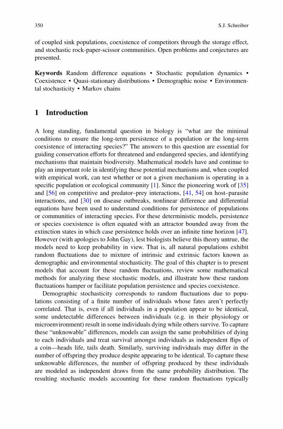
of coupled sink populations, coexistence of competitors through the storage effect,and stochastic rock-paper-scissor communities. Open problems and conjectures arepresented.
Keywords Random difference equations • Stochastic population dynamics •Coexistence • Quasi-stationary distributions • Demographic noise • Environmen-tal stochasticity • Markov chains
1 Introduction
A long standing, fundamental question in biology is “what are the minimalconditions to ensure the long-term persistence of a population or the long-termcoexistence of interacting species?” The answers to this question are essential forguiding conservation efforts for threatened and endangered species, and identifyingmechanisms that maintain biodiversity. Mathematical models have and continue toplay an important role in identifying these potential mechanisms and, when coupledwith empirical work, can test whether or not a given mechanism is operating in aspecific population or ecological community [1]. Since the pioneering work of [35]and [56] on competitive and predator–prey interactions, [41, 54] on host–parasiteinteractions, and [30] on disease outbreaks, nonlinear difference and differentialequations have been used to understand conditions for persistence of populationsor communities of interacting species. For these deterministic models, persistenceor species coexistence is often equated with an attractor bounded away from theextinction states in which case persistence holds over an infinite time horizon [47].However (with apologies to John Gay), lest biologists believe this theory untrue, themodels need to keep probability in view. That is, all natural populations exhibitrandom fluctuations due to mixture of intrinsic and extrinsic factors known asdemographic and environmental stochasticity. The goal of this chapter is to presentmodels that account for these random fluctuations, review some mathematicalmethods for analyzing these stochastic models, and illustrate how these randomfluctuations hamper or facilitate population persistence and species coexistence.
Demographic stochasticity corresponds to random fluctuations due to popu-lations consisting of a finite number of individuals whose fates aren’t perfectlycorrelated. That is, even if all individuals in a population appear to be identical,some undetectable differences between individuals (e.g. in their physiology ormicroenvironment) result in some individuals dying while others survive. To capturethese “unknowable” differences, models can assign the same probabilities of dyingto each individuals and treat survival amongst individuals as independent flips ofa coin—heads life, tails death. Similarly, surviving individuals may differ in thenumber of offspring they produce despite appearing to be identical. To capture theseunknowable differences, the number of offspring produced by these individualsare modeled as independent draws from the same probability distribution. Theresulting stochastic models accounting for these random fluctuations typically
Coexistence in the Face of Uncertainty 351
correspond to Markov chains on a finite or countable state space1 e.g. the numbers ofindividuals, 0; 1; 2; 3; : : : , in a population. When these models represent populationsor communities whose numbers tend to stay bounded and have no immigration,the populations in these models always go extinct in finite time [10]. Hence,unlike deterministic models, the asymptotic behavior of these stochastic modelsis trivial: eventually no one is left. This raises the following basic question aboutthe relationship between models accounting for demographic stochasticity and theirdeterministic counterparts:
“Any population allowing individual variation in reproduction, ultimately dies out–unlessit grows beyond all limits, an impossibility in a bounded world. Deterministic populationmathematics on the contrary allows stable asymptotics. Are these artifacts or do they tellus something interesting about quasi-stationary stages of real or stochastic populations?”—Peter [29]
As it turns out, there is a strong correspondence between the quasi-stationarybehavior of the stochastic models and the attractors of an appropriately definedmean-field model. Moreover, this correspondence highlights a universal scalingrelationship between extinction times and the size of the habitat where the specieslive. These results and their applications are the focus of the first half of this review.
While demographic stochasticity affects individuals independently, environ-mental stochasticity concerns correlated demographic responses (e.g. increasedsurvival, growth or reproduction) among individuals. These correlations often stemfrom individuals experiencing similar fluctuations in environmental conditions(e.g. temperature, precipitation, winds) which impact their survival, growth, orreproduction. Models driven by randomly fluctuating parameters or Brownianmotions, such as random difference equations or stochastic differential equations,can capture these sources of random fluctuations. Unlike models for demographicstochasticity, these Markov chains always live on uncountable state spaces wherethe non-negative reals represent densities of populations of sufficiently large sizethat one can ignore the effects of being discrete and finite. Consequently, like theirdeterministic counterparts, extinction in these random difference equations onlyoccurs asymptotically, and persistence is equated with tendency to stay away fromlow densities [11]. Understanding what this exactly means, reviewing methods forverifying this stochastic form of persistence, and applying these methods to gaininsights about population persistence and species coexistence are the focus of thesecond half of this review.
Of course, all population systems experience a mixture of demographic andenvironmental stochasticity. While the theoretical biology literature is replete withmodels accounting for each of these forms of noise separately, I know of no studiesthat rigorously blend the results presented in this review. Hence, I conclude bydiscussing some open problems and future challenges at this mathematical interface.
1See, however, the discussion for biologically motivated uncountable state spaces.

352 S.J. Schreiber
2 Demographic Stochasticity
To model finite populations and account for demographic stochasticity, we considerMarkov chains on a countable state space which usually is the non-negative cone ofthe integer lattice. Many of these stochastic models have a deterministic counterpart,sometimes called the “deterministic skeleton” or the “mean field model”. As Idiscuss below, these deterministic models can provide some useful insights about thetransient behavior of the stochastic models and when coupled with large deviationtheory provide insights into the length of these transients.
To get a flavor of the types of models being considered, lets begin with astochastic counterpart to the discrete-time Lotka-Volterra equations. This examplemotivates the main results and will illustrate their applicability.
Example 1 (Poisson Lotka-Volterra Processes) The continuous time Lotka-Volterra equations form the bedrock for much of community ecology theory. Whilethere are various formulations of their discrete-time counterparts, a particularlypleasing one that retains several key dynamical features of the continuous-timemodels was studied by [26]. These models keep track of the densities xt D.x1;t; : : : ; xk;t/ of k interacting species, where the subscripts denote the speciesidentity i and time t (e.g. year or day). As with the classical continuous timeequations, there is a matrix A D .aij/i;j where aij corresponds to the “per-capita”effect of species j on species i and a vector r D .r1; : : : ; rk/ of the “intrinsic per-capita growth rates” for all of the species. With this notation, the equations take onthe form:
xi;tC1 D xi;t exp
0@ri C
Xj
aijxj;t
1A DW Fi.xt/ with i D 1; 2; : : : ; k: (1)
The state space for these dynamics are given by the non-negative orthant
RkC D fx 2 R
k W xi � 0 for all ig
of the k-dimensional Euclidean space Rk.
To define the Poisson Lotka-Volterra process, let 1=" be the size of the habitatin which the species live. Let N"
t D .N"1;t; : : : ; N"
k;t/ denote the vector of speciesabundances which are integer-valued. Then the density of species i is X"
i;t D "N"i;t.
Over the next time step, each individual replaces itself with a Poisson number ofindividuals with mean
exp
0@ri C
Xj
aijX"j;t
1A :
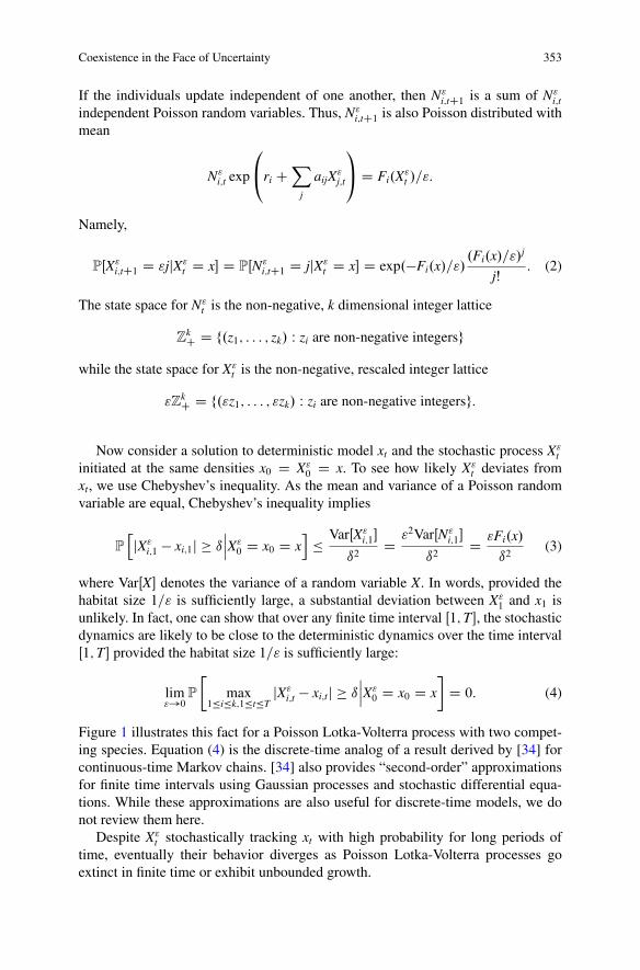
Coexistence in the Face of Uncertainty 353
If the individuals update independent of one another, then N"i;tC1 is a sum of N"
i;tindependent Poisson random variables. Thus, N"
i;tC1 is also Poisson distributed withmean
N"i;t exp
0@ri C
Xj
aijX"j;t
1A D Fi.X
"t /=":
Namely,
PŒX"i;tC1 D "jjX"
t D x� D PŒN"i;tC1 D jjX"
t D x� D exp.�Fi.x/="/.Fi.x/="/j
jŠ: (2)
The state space for N"t is the non-negative, k dimensional integer lattice
ZkC D f.z1; : : : ; zk/ W zi are non-negative integersg
while the state space for X"t is the non-negative, rescaled integer lattice
"ZkC D f."z1; : : : ; "zk/ W zi are non-negative integersg:
Now consider a solution to deterministic model xt and the stochastic process X"t
initiated at the same densities x0 D X"0 D x. To see how likely X"
t deviates fromxt, we use Chebyshev’s inequality. As the mean and variance of a Poisson randomvariable are equal, Chebyshev’s inequality implies
P
hjX"
i;1 � xi;1j � ıˇˇX"
0 D x0 D xi
� VarŒX"i;1�
ı2D "2VarŒN"
i;1�
ı2D "Fi.x/
ı2(3)
where VarŒX� denotes the variance of a random variable X. In words, provided thehabitat size 1=" is sufficiently large, a substantial deviation between X"
1 and x1 isunlikely. In fact, one can show that over any finite time interval Œ1; T�, the stochasticdynamics are likely to be close to the deterministic dynamics over the time intervalŒ1; T� provided the habitat size 1=" is sufficiently large:
lim"!0
P
�max
1�i�k;1�t�TjX"
i;t � xi;tj � ıˇˇX"
0 D x0 D x
�D 0: (4)
Figure 1 illustrates this fact for a Poisson Lotka-Volterra process with two compet-ing species. Equation (4) is the discrete-time analog of a result derived by [34] forcontinuous-time Markov chains. [34] also provides “second-order” approximationsfor finite time intervals using Gaussian processes and stochastic differential equa-tions. While these approximations are also useful for discrete-time models, we donot review them here.
Despite X"t stochastically tracking xt with high probability for long periods of
time, eventually their behavior diverges as Poisson Lotka-Volterra processes goextinct in finite time or exhibit unbounded growth.
354 S.J. Schreiber
020
40l
l
l l l l l l l l l l l l l l l l l l l l l l l l l l l l
l
l
l l l l l l l l l l l l l l l l l l l l l l l l l l l l
ε = 0.5
020
40
l
l
ll
l
ll
l
l
l
l
ll
l
l
l
l
l
l
l
l
l
ll
l
l
l
l
l
l
dens
ity
l
l
l l
l
ll
l
l l
l
l l
l
l
l
l
ll
l
l
l
l l l l l l l l
ε = 0.02
020
l
l
l
l
l
ll
l
ll
l
ll
l
ll
l
ll
l
l
l
l
l
l
l
ll
l
l
0 5 10 15 20 25 30
l
l
l l
l
l l
l
l l
l
l l
l
l l
l
l l
l
ll
l
ll
l
ll
l
l
ε = 0.001
0 5 10 15 20 25 30
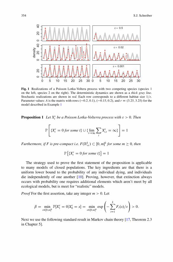
Fig. 1 Realizations of a Poisson Lotka-Voltera process with two competing species (species 1
on the left, species 2 on the right). The deterministic dynamics are shown as a thick gray line.Stochastic realizations are shown in red. Each row corresponds to a different habitat size 1=".Parameter values: A is the matrix with rows .�0:2; 0:1/, .�0:15; 0:2/, and r D .3:25; 3:25/ for themodel described in Example 1
Proposition 1 Let X"t be a Poisson Lotka-Volterra process with " > 0. Then
P
"fX"
t D 0 for some tg [ f limt!1
Xi
X"i;t D 1g
#D 1
Furthermore, if F is pre-compact i.e. F.RkC/ � Œ0; m�k for some m � 0, then
P�fX"
t D 0 for some tg� D 1
The strategy used to prove the first statement of the proposition is applicableto many models of closed populations. The key ingredients are that there is auniform lower bound to the probability of any individual dying, and individualsdie independently of one another [10]. Proving, however, that extinction alwaysoccurs with probability one requires additional elements which aren’t meet by allecological models, but is meet for “realistic” models.
Proof For the first assertion, take any integer m > 0. Let
ˇ D minx2Œ0;m�k
PŒX"1 D 0jX"
0 D x� D minx2Œ0;m�k
exp
�
kXiD1
Fi.x/="
!> 0:
Next we use the following standard result in Markov chain theory [17, Theorem 2.3in Chapter 5].

Coexistence in the Face of Uncertainty 355
Proposition 2 Let X be a Markov chain and suppose that
P
" 1[sD1
fXtCs 2 CgˇˇXt
#� ˇ > 0 on fXt 2 Bg:
Then
P ŒfXt enters B infinitely ofteng n fXt enters C infinitely ofteng� D 0:
Let Bm D fX"t enters Œ0; m�k infinitely ofteng and E D fX"
t D 0 for some tg.Proposition 2 with B D Œ0; m�k and C D f0g implies that
P ŒBm n E � D 0: (5)
The complement of the event [mBm equals the event A D flimt!1P
i X"i;t D 1g.
As Bm is an increasing sequence of events,
1 D P ŒA [ f[mBmg�D lim
m!1P ŒA [ Bm�
� limm!1P ŒA [ E �
where the final inequality follows from (5). This completes the proof of the firstassertion.
To prove the second assertion, assume that there exists m > 0 such that F.x/ 2Œ0; m�k for all x 2 R
kC i.e. F is pre-compact. Define
ˇ D infx2Rk
C
PŒX"tC1 D 0jXt D x�
D infx2Rk
C
exp
�X
i
Fi.x/="
!
� exp.�k m="/
Applying Proposition 2 with B D RkC and C D f0g completes the proof of the
second assertion. utEquation (4) and Proposition 1 raise two fundamental questions about these
stochastic, finite population models: How long before extinction occurs? Priorto extinction what can one say about the transient population dynamics? To getsome insights into both of these questions, we build on the work of [21] and[31] on random perturbations of dynamical systems, and [3] on quasi-stationarydistributions.

356 S.J. Schreiber
2.1 Random Perturbations and Quasi-Stationary Distributions
The Poisson Lotka-Volterra process (Example 1) illustrates how Markovian modelscan be viewed as random perturbations of a deterministic model. To generalize thisidea, consider a continuous, precompact2 map F W S ! S , where S is a closedsubset of Rk. F will be the deterministic skeleton of our stochastic models. A randomperturbation of F is a family of Markov chains fX"g">0 on S whose transitionkernels
p".x; � / D P�X"
tC1 2 � j X"t D x
�for all x 2 S and Borel sets � � S
enjoy the following hypothesis:
Hypothesis 2.1 For any ı > 0,
lim"!0
supx2S
p"�x;S n Nı.F.x//
� D 0
where Nı.y/ WD fx 2 S W ky � xk < ıg denotes the ı-neighborhood of a pointy 2 S .
Hypothesis 2.1 implies that the Markov chains X" converge to the deterministiclimit as " # 0 i.e. the probability of X"
1 being arbitrarily close to F.x/ given X"0 D x
is arbitrarily close to one for " sufficiently small. Hence, one can view F as the“deterministic skeleton” which gets clothed by the stochastic dynamic X". The nextexample illustrates how to verify the Poisson Lotka-Volterra process is a randomperturbation of the Lotka-Volterra difference equations.
Example 2 (The Poisson Lotka-Volterra Processes Revisited) Consider the PoissonLotka-Volterra processes from Example 1 where F.x/ D .F1.x/; : : : ; Fk.x// andFi.x/ D xi exp.ri CP
j aijxj/ and S D RkC. For many natural choices of ri and aij,
[26] have shown there exists C > 0 such that F.S / � Œ0; C�k i.e. F is pre-compact.While the corresponding Lotka-Volterra process X" lives on "ZkC, the process canbe extended to all of S by allowing X"
0 to be any point in S and update with thetransition probabilities of (2). With this extension, X"
1 always lies in "ZkC and p" ischaracterized by the following probabilities
p�.x; fyg/ DkY
iD1
exp.�Fi.x/="/.Fi.x/="/ji
jiŠfor y D ".j1; : : : ; jk/ 2 "ZkC; x 2 S
and 0 otherwise. With this extension, Hypothesis 1 for the Lotka-Volterra processfollows from equation (3).
2Namely, there exists C > 0 such that F.S / lies in Œ0; C�k.
Coexistence in the Face of Uncertainty 357
As with the Poisson Lotka-Volterra process, stochastic models of interacting pop-ulations without immigration always have absorbing states S0 � S correspondingto the loss of one or more populations. Hence, we restrict our attention to modelswhich satisfy the following standing hypothesis:
Hypothesis 2.2 The state space S can be written S D S0 [ SC, where
• S0 is a closed subset of S ;• S0 and SC are positively F-invariant, i.e F.S0/ � S0 and F.SC/ � SC;• the set S0 is assumed to be absorbing for the random perturbations:
p".x;SC/ D 0; for all " > 0; x 2 S0: (6)
� absorption occurs in finite time with probability one:
P�X"
t 2 S0 for some t � 1jX"0 D x
� D 1
for all x 2 S and " > 0.
The final bullet point implies that extinction of one or more species is inevitable infinite time. For example, Proposition 1 implies this hypothesis for Poisson Lotka-Volterra processes whenever F is pre-compact.
Despite this eventual absorption, the process X" may spend exceptionally longperiods of time in the set SC of transient states provided that " > 0 is sufficientlysmall. This “metastable” behavior may correspond to long-term persistence of anendemic disease, long-term coexistence of interacting species as in the case of thePoisson Lotka-Volterra process, or maintenance of a genetic polymorphism. Oneapproach to examining these metastable behaviors are quasi-stationary distributionswhich are invariant distributions when the process is conditioned on non-absorption.
Definition 1 A probability measure �" on SC is a quasi-stationary distribution(QSD) for p" provided there exists �" 2 .0; 1/ such that
ZSC
p".x; � /�".dx/ D �"�".� / for all Borel sets � � SC:
Equivalently, dropping the " superscript and subscripts, a QSD � satisfies theidentity
�.� / D P� ŒXt 2 � j Xt 2 SC� for all t;
where P� denotes the law of the Markov chain fXtg1tD0, conditional to X0 being
distributed according to �.In the case that the Markov chain has a finite number of states and P is the
transition matrix (i.e. Pij D p.i; fjg/), [15] showed that the QSD is given by�.fig/ D �i where � is the normalized, dominant left eigenvector of the matrixQ given by removing the rows and columns of P corresponding to extinction
358 S.J. Schreiber
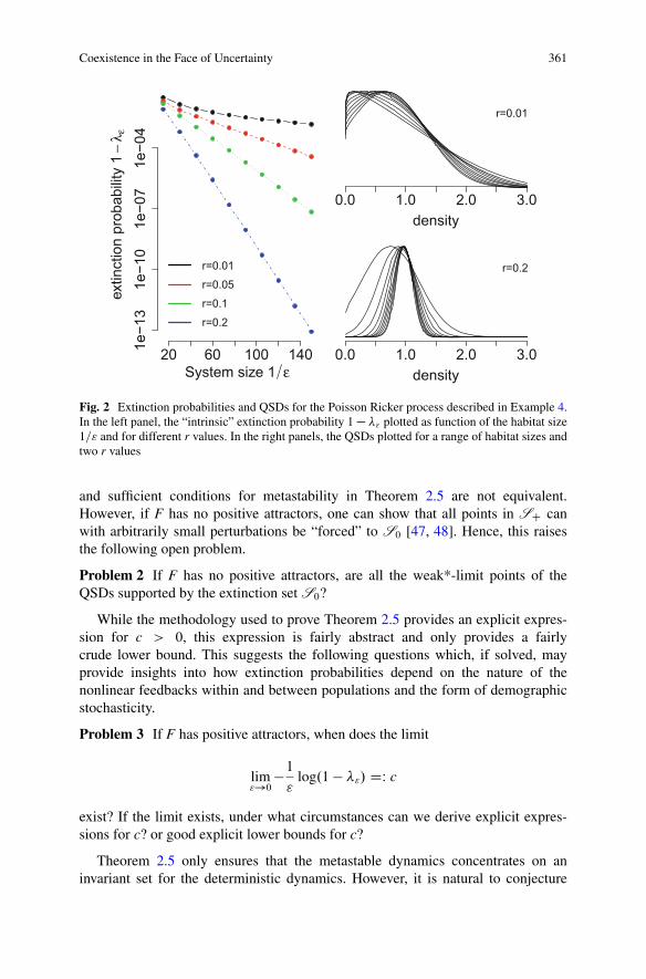
states in S0. In this case, � is the corresponding eigenvalue of this eigenvector.For the Poisson Lotka-Volterra processes in which the unperturbed dynamic F ispre-compact, Proposition 6.1 from [20] implies the existence of QSDs for theseprocesses. Examples of these QSDs for these processes are shown in Figs. 2, 3,and 4. More generally, the existence of QSDs has been studied extensively by manyauthors as reviewed by [39].
What do these QSD’s and � tell us about the behavior of the stochastic process?From the perspective of metastability, QSDs often exhibit the following property:
�.� / D limt!C1P ŒXt 2 � j Xt 2 SC; X0 D x�
where the limit exists and is independent of the initial state x 2 SC. In words, theQSD describes the probability distribution of Xt, conditioned on non-extinction, farinto the future. Hence, the QSD provides a statistical description of the meta-stablebehavior of the process. The eigenvalue, � provides information about the length ofthe metastable behavior of Xt. Specifically, given that the process is following theQSD (e.g. X0 is distributed like �), and � equals the probability of persisting in thenext time step. Thus, the mean time to extinction is 1
1��. [22] call 1
1��, the “intrinsic
mean time to extinction” and, convincingly, argue that it is a fundamental statisticfor comparing extinction risk across stochastic models.
2.2 Positive Attractors, Intrinsic Extinction Risk, andMetastability
When the habitat size is sufficiently large i.e. " is small, there is a strongrelationship between the existence of attractors in SC (i.e. “positive” attractors)for the unperturbed system F and the quasi-stationary distributions of X". Thisrelationship simultaneously provides information about the metastable behavior ofthe stochastic model and intrinsic probability of extinction, 1 � �". To make thisrelationship mathematically rigorous, we need to strengthen Hypotheses 2.1 and 2.2.[20] presents two ways to strengthen these hypothesis. We focus on their largedeviation approach as it is most easily verified. This approach requires identifying arate function � W S �S ! Œ0; 1� that describes the probability of a large deviationbetween F and X". That is, for a sufficiently small neighborhood U of a point y, therate function should have the property
PŒX"tC1 2 UjX"
t D x� exp.��.x; y/="/:
Hypothesis 2.3 provides the precise definition and desired properties of �.
Hypothesis 2.3 There exists a rate function � W S � S ! Œ0; C1� such that
(i) � is continuous on SC � S ,
Coexistence in the Face of Uncertainty 359
(ii) �.x; y/ D 0 if and only if y D F.x/,(iii) for any ˇ > 0,
inf f�.x; y/ W x 2 S ; y 2 S ; kF.x/ � yk > ˇg > 0; (7)
(iv) for any open set U, there is the lower bound
lim inf"!0
" log p".x; U/ � � infy2U
�.x; y/ (8)
that holds uniformly for x in compact subsets of SC whenever U is an openball in S . Additionally, for any closed set C, there is the uniform upper bound
lim sup"!0
supx2S
" log p".x; C/ � � infy2C
�.x; y/: (9)
Equations (7) and (9), in particular, imply that Hypothesis 2.1 holds. Furthermore,as S0 is absorbing, equation (8) implies that �.x; y/ D C1 for all x 2 S0, y 2 SC.Identifying the rate function � typically requires making use of the Gärtner-Ellistheorem [16, Theorem 2.3.6] which provides large deviation estimates for sums ofindependent random variables. Example 3 below describes how this theorem wasused for the Poisson Lotka-Volterra processes.
We strengthen Hypothesis 2.2 as follows:
Hypothesis 2.4 For any c > 0, there exists an open neighborhood V0 of S0 suchthat
lim"!0
infx2V0
" log p".x;S0/ � �c: (10)
Equation (10) implies that
PŒX"tC1 2 S0jXt 2 V0� � exp.�c="/
for " > 0 sufficiently small. Namely, the probability of absorption near theboundary, at most, decays exponentially with habitat size. The following examplediscusses why these stronger hypotheses hold for the Poisson Lotka-Volterraprocess.
Example 3 (Return of the Poisson Lotka-Volterra Process) Using the Gärtner-Ellistheorem [16, Theorem 2.3.6], Faure and Schreiber [20, Proposition 6.4] showed that�.x; y/ D P
i yi log yiFi.x/
�yi is the rate function for any Poisson processes with mean
F W RkC ! RkC including the Poisson Lotka-Volterra Process of Example 1. To see
why Hypothesis 4 holds for the Poisson Lotka-Volterra process, assume x is suchthat xi � ı for some ı > 0 and i. Then
" logPŒX"tC1 2 S0jXt D x� � " logPŒX"
i;tC1 D 0jXt D x�
D " log exp.�Fi.x/="/ D �Fi.x/

360 S.J. Schreiber
Hence, for any c > 0, choose ı > 0 sufficiently small to ensure that for all i,Fi.x/ � c whenever xi � ı. In which case, choosing V0 D fx 2 R
kC W xi � ı forsome ig satisfies (10).
As many discrete distributions are used in models with demographic stochas-ticity (e.g. negative binomial, mixtures of Bernoullis and negative binomials), animportant open problem is the following:
Problem 1 For which types of random perturbations of an ecological model F doHypotheses 3 and 4 hold?
To relate QSDs to the attractors of the deterministic dynamics, we recall thedefinition of an attractor and weak* convergence of probability measures. Acompact set A � S is an attractor for F if there exists a neighborhood U of Asuch that (i) \n�1Fn.U/ D A and (ii) for any open set V containing A, Fn.U/ � Vfor some n � 1. A weak* limit point of a family of probability measures f�"g">0 onS is a probability measure �0 such that there exists a sequence "n # 0 satisfying
limn!1
Zh.x/�"n.dx/ D
Zh.x/�0.dx/
for all continuous functions h W S ! R. Namely, the expectation of any continuousfunction with respect to �"n converges to its expectation with respect to �0 asn ! 1. The following theorem follows from [20, Lemma 3.9 and Theorem 3.12].
Theorem 2.5 Assume Hypotheses 2.3 and 2.4 hold. Assume for each " > 0, thereexists a QSD �" for X". If there exists a positive attractor A � SC, then
• there exists a neighborhood V0 of S0 such that all weak* limit points �0 off�"g">0 are F-invariant and �0.V0/ D 0, and
• there exists c > 0 such that
�" � 1 � e�c=" for all " > 0: (11)
Alternatively, assume that S0 is a global attractor for the dynamics of F. Then anyweak*-limit point of f�"g">0 is supported by S0.
Theorem 2.5 implies the existence of a positive attractor of the deterministicdynamics ensures the stochastic process exhibits metastable behavior for largehabitat size, and the probability of extinction 1 � �" decreases exponentiallywith habitat size. Equivalently, the mean time to extinction 1=.1 � �"/ increasesexponential with habitat size. These conclusions are illustrated in Fig. 2 with a one-dimensional Poisson Lotka-Volterra process (the Poisson Ricker process describedbelow in Example 4).
Even if F has no positive attractors, S0 may not be a global attractor as theremight be an unstable invariant set in SC. For example, single species models withpositive feedbacks can have an uncountable number of unstable periodic orbitsdespite almost every initial condition going to extinction [46]. Hence, the necessary
Coexistence in the Face of Uncertainty 361
20 60 100 1401e−1
31e
−10
1e−0
71e
−04
System size 1 ε
extin
ctio
n pr
obab
ility
1−
λ ε
r=0.01
r=0.05
r=0.1
r=0.2
0.0 1.0 2.0 3.0density
r=0.2
0.0 1.0 2.0 3.0density
r=0.01
Fig. 2 Extinction probabilities and QSDs for the Poisson Ricker process described in Example 4.In the left panel, the “intrinsic” extinction probability 1 � �" plotted as function of the habitat size1=" and for different r values. In the right panels, the QSDs plotted for a range of habitat sizes andtwo r values
and sufficient conditions for metastability in Theorem 2.5 are not equivalent.However, if F has no positive attractors, one can show that all points in SC canwith arbitrarily small perturbations be “forced” to S0 [47, 48]. Hence, this raisesthe following open problem.
Problem 2 If F has no positive attractors, are all the weak*-limit points of theQSDs supported by the extinction set S0?
While the methodology used to prove Theorem 2.5 provides an explicit expres-sion for c > 0, this expression is fairly abstract and only provides a fairlycrude lower bound. This suggests the following questions which, if solved, mayprovide insights into how extinction probabilities depend on the nature of thenonlinear feedbacks within and between populations and the form of demographicstochasticity.
Problem 3 If F has positive attractors, when does the limit
lim"!0
�1
"log.1 � �"/ DW c
exist? If the limit exists, under what circumstances can we derive explicit expres-sions for c? or good explicit lower bounds for c?
Theorem 2.5 only ensures that the metastable dynamics concentrates on aninvariant set for the deterministic dynamics. However, it is natural to conjecture
362 S.J. Schreiber
0.0 0.5 1.0 1.5 2.0 2.5 3.0density
r=1.9
0.0 0.5 1.0 1.5 2.0 2.5 3.0density
r=2.1
0.0 0.5 1.0 1.5 2.0 2.5 3.0density
r=2.6
0.0 0.5 1.0 1.5 2.0 2.5 3.0density
r=3.15
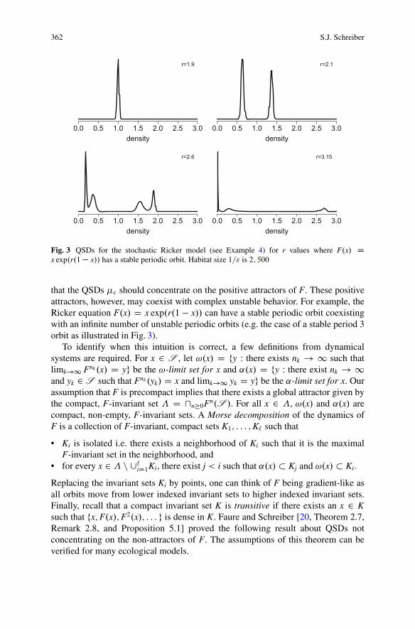
Fig. 3 QSDs for the stochastic Ricker model (see Example 4) for r values where F.x/ Dx exp.r.1 � x// has a stable periodic orbit. Habitat size 1=" is 2; 500
that the QSDs �" should concentrate on the positive attractors of F. These positiveattractors, however, may coexist with complex unstable behavior. For example, theRicker equation F.x/ D x exp.r.1 � x// can have a stable periodic orbit coexistingwith an infinite number of unstable periodic orbits (e.g. the case of a stable period 3
orbit as illustrated in Fig. 3).To identify when this intuition is correct, a few definitions from dynamical
systems are required. For x 2 S , let !.x/ D fy W there exists nk ! 1 such thatlimk!1 Fnk .x/ D yg be the !-limit set for x and ˛.x/ D fy W there exist nk ! 1and yk 2 S such that Fnk .yk/ D x and limk!1 yk D yg be the ˛-limit set for x. Ourassumption that F is precompact implies that there exists a global attractor given bythe compact, F-invariant set D \n�0Fn.S /. For all x 2 , !.x/ and ˛.x/ arecompact, non-empty, F-invariant sets. A Morse decomposition of the dynamics ofF is a collection of F-invariant, compact sets K1; : : : ; K` such that
• Ki is isolated i.e. there exists a neighborhood of Ki such that it is the maximalF-invariant set in the neighborhood, and
• for every x 2 n [`iD1Ki, there exist j < i such that ˛.x/ � Kj and !.x/ � Ki.
Replacing the invariant sets Ki by points, one can think of F being gradient-like asall orbits move from lower indexed invariant sets to higher indexed invariant sets.Finally, recall that a compact invariant set K is transitive if there exists an x 2 Ksuch that fx; F.x/; F2.x/; : : : g is dense in K. Faure and Schreiber [20, Theorem 2.7,Remark 2.8, and Proposition 5.1] proved the following result about QSDs notconcentrating on the non-attractors of F. The assumptions of this theorem can beverified for many ecological models.
Coexistence in the Face of Uncertainty 363
Theorem 2.6 Assume Hypotheses 2.3 and 2.4 hold. Let K1; : : : ; K` be a Morsedecomposition for F such Kj; : : : ; K` are attractors. If
• Ki � SC or Ki � S0 for each i,• Ki � SC for some i � j, and• Ki with i � j � 1 is transitive whenever Ki � SC,
then any weak*-limit point of f�"g">0 is F-invariant and is supported by the unionof attractors in SC.
For random perturbations of deterministic models without absorbing states (e.g.models accounting for immigration or mutations between genotypes), the work of[31] and [21] can be used to show that the stationary distributions often concentrateon a unique attractor. However, due to the singularity of the rate function � alongthe extinction set S0, the approach used by these authors doesn’t readily extend tothe stochastic models considered here. This raises the following open problem:
Problem 4 If F has multiple, positive attractors, under what conditions do theQSDs �" concentrate on a unique one of these positive attractors as " # 0?
Lets apply some of these results to the Poisson Lotka-Volterra processes fromExample 1.
Example 4 (The Ricker Model) The simplest of Poisson Lotka-Volterra processesis the stochastic Ricker model for a single species where F.x/ D x exp.r.1 � x//
with r > 0. [33] proved that for an open and dense set of r > 0 values, theRicker map has a Morse decomposition consisting of a finite number of unstable,intransitive sets (more specifically, hyperbolic sets) and a unique stable period orbitfp; F.p/; : : : ; FT.p/g. As the stable periodic orbit is the only attractor, Theorem 2.6implies the following result.
Corollary 1 Consider the Ricker process with r > 0 such that F.x/ D x exp.r.1�x// has the aforementioned Morse decomposition. Then any weak*-limit pointof f�"g">0 is supported by the unique stable periodic orbit fp; F.p/; : : : ; FT.p/g.
Figure 3 illustrates this corollary: QSDs concentrating on the stable periodic orbitof period 1 for r D 1:9, period 2 for r D 2:1, period 4 for r D 2:6, and period 3
for r D 3:15. Remarkably, in the case of the stable orbit of period 3, there exists aninfinite number of unstable periodic orbits which the QSDs do not concentrate on.We note that [27, 32, 42] proved similar results to Corollary 1 using inherently onedimensional methods.
Example 5 (Revenge of the Poisson Lotka-Volterra Processes) For higher dimen-sional Lotka-Volterra processes, we can use properties of Lotka-Volterra differenceequations in conjunctions with Theorems 2.5 and 2.6 to derive two algebraicallyverifiable results for the stochastic models. First, if the deterministic map F D.F1; : : : ; Fk/ with Fi.x/ D xi exp.
Pj Aijxj C ri/ is pre-compact and there is no
internal fixed point (i.e. there is no strictly positive solution to Ax D �r), then[26] proved that the boundary of the positive orthant is a global attractor. Hence,Theorem 2.5 implies the following corollary.

364 S.J. Schreiber
Corollary 2 Let X" be a Poisson Lotka-Volterra process such that F is pre-compactand admits no positive fixed point. Then any weak*-limit point of f�"g">0 issupported by S0, the boundary of the positive orthant of RkC.
On the other hand, [26] derived a simple algebraic condition which ensures thatthe deterministic dynamics of F has a positive attractor. Namely, there exist pi > 0
such that
Xi
pi
0@X
j
Aijx�j C ri
1A > 0 (12)
for any fixed point x� on the boundary of the positive orthant. Hence, Theorem 2.5implies the following corollary.
Corollary 3 Assume F D .F1; : : : ; Fk/ with Fi.x/ D xi exp.P
j Aijxj C ri/ is pre-compact and satisfies (12) for some choice of pi > 0. If X" is the correspondingPoisson Lotka-Volterra process, then any weak*-limit point of f�"g">0 is supportedby A where A � SC is the global, positive attractor for F. Moreover, there existsc > 0 such that �" � 1 � exp.c="/ for all " > 0 sufficiently small.
Figure 4 illustrates the convergence of the QSDs to the attractor of F for a Lotka-Volterra process of two competing species. Even for populations of only hundredsof individuals (" D 0:01), this figure illustrates that species can coexist for tens ofthousands of generations despite oscillating between low and high densities, a keysignature of the underlying deterministic dynamics. However, only at much largerhabitat sizes (e.g. 1=" D 1; 000; 000) do the metastable behaviors clearly articulatethe underlying deterministic complexities.
3 Environmental Stochasticity
To understand how environmental fluctuations, in and of themselves, influencepopulation dynamics, we shift our attention to models for which the habitat sizeis sufficiently large that one can approximate the population state by a continuousvariable. Specifically, let Xt 2 R
kC denote the state of the population or communityat time t. The components of Xt D .X1;t; X2;t; : : : ; Xk;t/ corresponds to densitiesor frequencies of subpopulations. To account for environmental fluctuations, letE � R
m (for some m) be a compact set representing all possible environmentalstates e.g. all possible precipitation and temperature values. I assume that EtC1 2 Erepresents the environmental state of the system over the time interval .t; t C 1�
that determines how the community state changes over that time interval. If thepopulation or community state XtC1 depends continuously on EtC1 and Xt, then
XtC1 D F.Xt; EtC1/ (13)

Coexistence in the Face of Uncertainty 365
ε = 0.01 ε = 1e−04
ε = 1e−06 deterministic F
Fig. 4 Numerically estimated QSDs for a Poisson Lotka-Volterra process with two competingspecies, and the global attractor of the deterministic map Fi.x/ D xi exp.
Pj Aijxjx C ri/. The
stochastic and deterministic processes were simulated for 50; 000 time steps and the last 17,500time steps are plotted in the x1–x2 plane. Parameters: A is the matrix with rows .�0:2; �0:01/,.�0:01; �0:2/ and r D .2:71; 2:71/
for a continuous map F W RkC �E ! RkC. If the Et are random variables, then (13) is
known as a continuous, random dynamical system. [2] provides a thorough overviewof the general theory of these random dynamical systems.
To state the main hypotheses about (13), recall that a sequence of randomvariables, E1; E2; : : : ; is stationary if for every pair of non-negative integers t and s,E1; : : : ; Et and E1Cs; : : : ; EtCs have the same distribution. The sequence is ergodicif with probability one all realizations of the sequence have the same asymptoticstatistical properties e.g. time averages (see, e.g., [17] for a more precise definition).
Hypothesis 3.7 E1; E2; : : : are an ergodic and stationary sequence of randomvariables taking value in E . Let � be the stationary distribution of this sequencei.e. the probability measure � on E such that PŒEt 2 B� D �.B/ for all Borelsets B � E .
This hypothesis is satisfied for a diversity of models of environmental dynamics.For example, Et could be given by a finite state Markov chain on a finite number
366 S.J. Schreiber
of environmental states, say e1; e2; : : : ; em 2 E (e.g. wet and cool, wet and hot,dry and cool, dry and hot) with transition probabilities pij D PŒEtC1 D ejjEt Dei�. If the transition matrix P D .pij/i;j is aperiodic and irreducible, then Et isasymptotically ergodic and stationary. Alternatively, Et could be given by a sequenceof independent and identically distributed random variables or, more generally, anautoregressive process.
Our second hypothesis simply assumes that population densities remain boundedand allows for the possibility of extinction.
Hypothesis 3.8 There are compact sets S � RkC and S0 � fx 2 S W Qi xi D 0g
such that F W S � E ! S , F W S0 � E ! S0, and F W SC � E ! SC whereSC D S n S0.
For example, S may equal Œ0; M�k where M is the maximal density of a speciesor S may be the probability simplex D fx 2 R
kC W Pi xi D 1g where x 2 Scorresponds to the vector of genotypic frequencies. As in the case of demographicstochasticity, S0 corresponds to the set where one or more populations have goneextinct. Invariance of S0 implies that once the population has gone extinct itremains extinct i.e. the “no cats, no kittens” principle. Invariance of SC implies thatpopulations can not go extinct in one time step but only asymptotically. This latterassumption is met by most (but not all) models in the population biology literature.
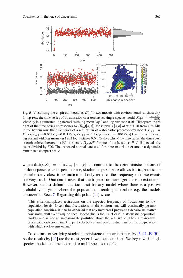
For these stochastic difference equations, there are several concepts of “per-sistence” which are reviewed in [49]. Here, we focus on the “typical trajectory”perspective. Namely, “how frequently does the typical population trajectory visita particular configuration of the population state space far into the future?” Theanswer to this question is characterized by empirical measures for Xt:
˘ xt .A/ D #f0 � s � t W Xs 2 Ag
t C 1
where X0 D x and A is a Borel subset of S . ˘t.A/ equals the fraction of time thatXs spends in the set A over the time interval Œ0; t�. Provided the limit exists, the long-term frequency that Xt enters A is given by limt!1 ˘ x
t .A/. It is important to notethat these empirical measures are random measures as they depend on the particularrealization of the stochastic process. Figure 5 provides graphical illustrations ofempirical measures for a single species model (top row) and a two species model(bottom row). For both models, the empirical measure at time t can be approximatedby a histogram describing the frequency Xt spends in different parts (e.g. intervalsor hexagons) of the population state space S .
Stochastic persistence corresponds to the typical trajectory spending arbitrarilylittle time, arbitrarily near the extinction set S0. More precisely, for all " > 0 thereexists a ı > 0 such that
lim supt!1
˘ xt .fx 2 S W dist.x;S0/ � ıg/ � " with probability one for all x 2 SC
Coexistence in the Face of Uncertainty 367
lllll
l
l
l
l
l
ll
ll
ll
lll
l
lll
l
llll
ll
ll
l
ll
l
l
llllll
l
lllll
l
l
l
l
lllllll
l
l
l
lll
ll
l
llll
l
ll
l
ll
ll
llllll
lll
ll
lll
lllllllll
l
l
lllllll
lll
l
ll
lllllll
ll
llll
l
lll
lll
l
ll
llll
lll
l
l
ll
llllll
l
ll
l
llllllllll
l
lll
lllll
l
ll
ll
ll
ll
lll
l
l
lll
lll
l
l
l
l
l
llll
l
l
ll
ll
l
llll
ll
l
l
llllllllll
ll
l
llll
llll
ll
lll
llll
l
llllll
l
l
llll
l
l
l
l
ll
l
llllllllll
l
llll
lllll
l
l
l
l
l
lllllll
ll
l
l
ll
lllll
l
lllll
ll
l
llll
l
l
ll
ll
ll
l
ll
l
l
l
l
ll
l
lllll
l
ll
ll
ll
l
lll
l
l
ll
l
lll
llllllllllll
l
l
lllll
l
llll
l
lll
lllllll
l
l
ll
ll
ll
lll
l
l
l
ll
l
l
l
l
lll
lllllll
ll
l
ll
ll
lllll
l
lll
lll
lll
l
l
ll
l
lll
lllll
l
llll
l
ll
l
lll
ll
lll
l
lll
l
llll
0 100 200 300 400 500
040
8012
0
time
abun
danc
e
llllll
l
l
l
ll
l
l
l
ll
l
ll
l
lll
l
l
ll
llll
l
ll
l
l
l
l
l
l
llllll
l
ll
ll
l
lllllll
l
llll
lll
ll
lll
l
l
llll
ll
ll
l
lll
l
l
l
l
lll
l
l
ll
l
l
l
l
l
l
l
l
ll
l
l
ll
l
ll
ll
l
l
l
ll
l
l
l
l
l
ll
l
l
l
l
ll
l
l
l
l
l
l
lll
llllll
l
l
l
ll
ll
lll
l
ll
l
ll
l
l
l
l
l
ll
l
ll
l
l
l
ll
l
l
ll
l
l
l
lll
l
l
ll
l
l
llllll
l
l
ll
l
l
l
l
l
l
l
l
lll
l
lll
l
l
ll
lllll
l
l
l
l
l
lll
ll
l
l
ll
lll
ll
l
l
l
l
l
l
l
l
ll
ll
l
l
l
l
lll
l
l
lll
l
l
l
l
ll
l
lll
llll
l
ll
l
l
ll
l
l
l
lll
l
ll
lll
l
l
l
ll
l
l
l
l
llll
ll
ll
l
l
llllll
ll
l
l
l
l
l
l
l
l
l
l
l
l
l
l
l
l
l
l
l
l
l
lllll
l
l
l
l
l
ll
l
ll
ll
l
ll
l
l
l
ll
lll
ll
l
l
l
l
l
ll
l
lll
ll
ll
llll
l
l
ll
l
l
l
lll
l
l
l
l
l
lll
l
ll
l
l
l
lll
l
ll
l
l
l
l
l
l
llll
ll
l
ll
l
lll
l
ll
l
ll
ll
ll
l
ll
l
l
l
l
l
l
ll
ll
l
l
lll
l
ll
lll
l
l
l
l
l
l
l
l
l
l
l
lll
lllll
l
ll
l
ll
l
l
ll
l
l
l
l
l
l
ll
l
0 100 200 300 400 500
020
060
010
00
time
abun
danc
e
Abundance of species 1A
bund
ance
of s
peci
es 2
100
200
300
400
200 400 600 800 1000
Counts
124477094117140163186209232255278302325348371
Fig. 5 Visualizing the empirical measures ˘ xt for two models with environmental stochasticity.
In top row, the time series of a realization of a stochastic, single species model XtC1 D �tC1Xt
1C0:01Xtwhere �t is a truncated log normal with log-mean log 2 and log-variance 0:01. Histogram to theright of the time series corresponds to ˘ x
500.Œa; b�/ for intervals Œa; b� of width 10 from 0 to 140.In the bottom row, the time series of a realization of a stochastic predator-prey model X1;tC1 DX1;t exp.�tC1�0:001X1;t �0:001X2;t/, X2;tC1 D 0:5X1;t.1�exp.�0:001X2;t// here �t is a truncatedlog normal with log-mean log 2 and log-variance 0:04. To the right of the time series, the time spentin each colored hexagon in R
2C
is shown. ˘ x500.H/ for one of the hexagons H � R
2C
equals thecount divided by 500. The truncated normals are used for these models to ensure that dynamicsremain in a compact set S
where dist.x; S0/ D miny2S0 kx � yk. In contrast to the deterministic notions ofuniform persistence or permanence, stochastic persistence allows for trajectories toget arbitrarily close to extinction and only requires the frequency of these eventsare very small. One could insist that the trajectories never get close to extinction.However, such a definition is too strict for any model where there is a positiveprobability of years where the population is tending to decline e.g. the modelsdiscussed in Sect. 7. Regarding this point, [11] wrote
“This criterion. . . places restrictions on the expected frequency of fluctuations to lowpopulation levels. Given that fluctuations in the environment will continually perturbpopulation densities, it is to be expected that any nominated population density, no matterhow small, will eventually be seen. Indeed this is the usual case in stochastic populationmodels and is not an unreasonable postulate about the real world. Thus a reasonablepersistence criterion cannot hope to do better than place restrictions on the frequencieswith which such events occur.”
Conditions for verifying stochastic persistence appear in papers by [5, 44, 49, 50].As the results by [44] are the most general, we focus on them. We begin with singlespecies models and then expand to multi-species models.

368 S.J. Schreiber
3.1 Single Species Models
Consider a single species for which an individual can be in one of k states.For example, these states may correspond to age where k is the maximal age,living in one of k spatial locations or “patches”, discrete behavioral states thatan individual can move between, different genotypes in an asexual populationcoupled by mutation, or finite number of developmental stages or size classes. Xi;t
corresponds to population density of individuals in state i and Xt D .X1;t; : : : ; Xk;t/
is the population state. The population state is updated by multiplication by a k � kmatrix A.Xt; EtC1/ dependent on the population and environmental state:
XtC1 D A.Xt; EtC1/Xt DW F.Xt; EtC1/: (14)
Assume A.X; E/ satisfies the following hypothesis.
Hypothesis 3.9 A is a continuous mapping from S � E to non-negative k � kmatrices. Furthermore, there exists a non-negative, primitive matrix B such thatA.x; E/ has the same sign structure as B for all x; E i.e. the i–j-th entry of A.x; E/ ispositive if and only if the i–j-th entry of B is positive.
The primitivity assumption implies that there is a time, T , such that after Ttime steps, individuals in every state contribute to individuals in all other states.Specifically, A.XT�1; ET/A.XT�2; ET�1/ : : : A.X0; E1/ has only positive entries forany X0; : : : ; XT�1 2 S and E1; : : : ; ET 2 E . This assumption is met for mostmodels.
To determine whether or not the population has a tendency to increase or decreasewhen rare, we can approximate the dynamics of (14) when X0 0 by the linearizedsystem
ZtC1 D BtC1Zt where Z0 D X0 and BtC1 D A.0; EtC1/: (15)
Iterating this matrix equation gives
Zt D BtBt�1Bt�2 : : : B2B1Z0:
Proposition 3.2 from [45] and Birkhoff’s ergodic theorem implies there is a quantityr, the dominant Lyapunov exponent, such that
limt!1
1
tlog kZtk D r with probability one
whenever Z0 2 RkC n f0g. Following [7–9], we call r the low-density per-capita
growth of the population. When r > 0, Zt with probability one grows exponentiallyand we would expect the population state Xt to increase when rare. Conversely whenr < 0, Zt with probability one converges to 0. Consistent with these predictionsfrom the linear approximation, Roth and Schreiber [44, Theorems 3.1,5.1] provedthe following result.
Coexistence in the Face of Uncertainty 369
Theorem 3.10 Assume Hypotheses 3.7 through 3.9 hold with S0 D f0g. If r > 0,then (14) is stochastically persistent. If r < 0 and A.0; E/ � A.X; E/ for all X; E,then
limt!1 Xt D 0 with probability one.
The assumption in the partial converse is a weak form of negative-densitydependence as it requires that the best conditions (in terms of magnitude of theentries of A) occurs at low densities. There are cases where this might not be true e.g.models accounting for positive density-dependence, size structured models wheregrowth to the next stage is maximal at low densities.
Example 6 (The Case of the Bay Checkerspot Butterflies) The simplest case forwhich Theorem 3.10 applies are unstructured models where k D 1. In this case,Bt D A.0; Et/ are scalars and
r D EŒlog Bt�:
The exponential er corresponds to the geometric mean of the Bt. By Jensen’sinequality, the arithmetic mean EŒBt� is greater than or equal to this geometric meaner, with equality only if Bt is constant with probability one. Hence, environmentalfluctuations in the low-density fitnesses Bt reduce r and have a detrimental effect onpopulation persistence.
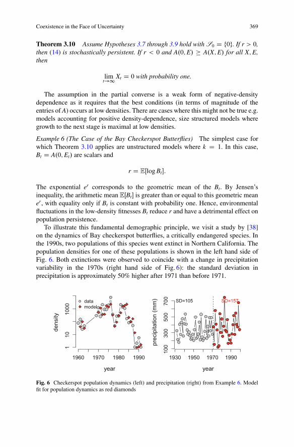
To illustrate this fundamental demographic principle, we visit a study by [38]on the dynamics of Bay checkerspot butterflies, a critically endangered species. Inthe 1990s, two populations of this species went extinct in Northern California. Thepopulation densities for one of these populations is shown in the left hand side ofFig. 6. Both extinctions were observed to coincide with a change in precipitationvariability in the 1970s (right hand side of Fig. 6): the standard deviation inprecipitation is approximately 50% higher after 1971 than before 1971.
1960 1970 1980 1990
110
1000
year
dens
ity
datamodel
1930 1950 1970 1990
100
300
500
700
year
prec
ipita
tion
(mm
) SD=105 SD=157
Fig. 6 Checkerspot population dynamics (left) and precipitation (right) from Example 6. Modelfit for population dynamics as red diamonds
370 S.J. Schreiber
0 50 150
110
0
pre−1971 rainfall
year
dens
ity
0 50 150
110
0
post−1971 rainfall
year
dens
ity
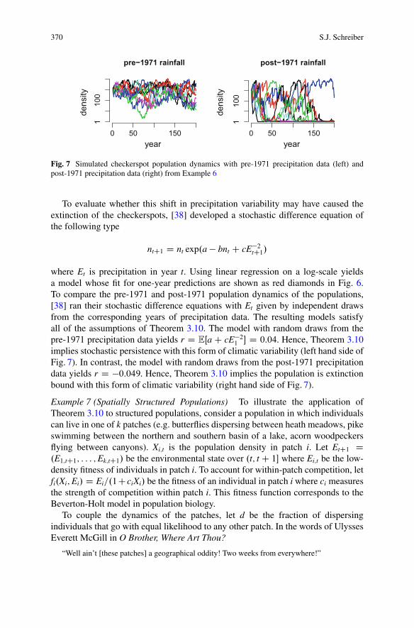
Fig. 7 Simulated checkerspot population dynamics with pre-1971 precipitation data (left) andpost-1971 precipitation data (right) from Example 6
To evaluate whether this shift in precipitation variability may have caused theextinction of the checkerspots, [38] developed a stochastic difference equation ofthe following type
ntC1 D nt exp.a � bnt C cE�2tC1/
where Et is precipitation in year t. Using linear regression on a log-scale yieldsa model whose fit for one-year predictions are shown as red diamonds in Fig. 6.To compare the pre-1971 and post-1971 population dynamics of the populations,[38] ran their stochastic difference equations with Et given by independent drawsfrom the corresponding years of precipitation data. The resulting models satisfyall of the assumptions of Theorem 3.10. The model with random draws from thepre-1971 precipitation data yields r D EŒa C cE�2
1 � D 0:04. Hence, Theorem 3.10implies stochastic persistence with this form of climatic variability (left hand side ofFig. 7). In contrast, the model with random draws from the post-1971 precipitationdata yields r D �0:049. Hence, Theorem 3.10 implies the population is extinctionbound with this form of climatic variability (right hand side of Fig. 7).
Example 7 (Spatially Structured Populations) To illustrate the application ofTheorem 3.10 to structured populations, consider a population in which individualscan live in one of k patches (e.g. butterflies dispersing between heath meadows, pikeswimming between the northern and southern basin of a lake, acorn woodpeckersflying between canyons). Xi;t is the population density in patch i. Let EtC1 D.E1;tC1; : : : ; Ek;tC1/ be the environmental state over .t; t C 1� where Ei;t be the low-density fitness of individuals in patch i. To account for within-patch competition, letfi.Xi; Ei/ D Ei=.1CciXi/ be the fitness of an individual in patch i where ci measuresthe strength of competition within patch i. This fitness function corresponds to theBeverton-Holt model in population biology.
To couple the dynamics of the patches, let d be the fraction of dispersingindividuals that go with equal likelihood to any other patch. In the words of UlyssesEverett McGill in O Brother, Where Art Thou?
“Well ain’t [these patches] a geographical oddity! Two weeks from everywhere!”

Coexistence in the Face of Uncertainty 371
Despite this odd geographic regularity, these all-to-all coupling models have provenvaluable to understanding spatial population dynamics. Under these assumptions,we get a spatially structured model of the form
Xi;tC1 D .1 � d/fi.Xi;t; Ei;tC1/Xi;t C d
k � 1
Xj¤i
fj.Xj;t; Ej;tC1/Xj;t: (16)
For this model, A.X; E/ is the matrix whose i–j-th entry equals dk�1
fj.Xj;t; Ej;tC1/ forj ¤ i and .1 � d/fi.Xi;t; Ei;tC1/ for j D i.
The low density per-capita growth rate r is the dominant Lyapunov exponent ofthe random product of the matrices Bt D A.0; Et/. Theorem 3.10 implies this modelexhibits stochastic persistence if r > 0 and asymptotic extinction with probabilityone if r < 0. In fact, as this spatial model has some special properties (monotonicityand sublinearity), work of Benaïm and Schreiber [5, Theorem 1] implies if r > 0,then there is a probability measure m on SC such that
limT!1
1
T
TXtD1
h.Xt/ DZ
h.x/ m.dx/ with probability one
for any x 2 SC and any continuous function h W S ! R. Namely, for allpositive initial conditions, the long-term behavior is statistically characterized by theprobability measure m that places no weight on the extinction set. When this occurs,running the model once for sufficiently long describes the long-term statisticalbehavior for all runs with probability one. The probability measure m correspondsto the marginal of an invariant measure for the stochastic model.
But when is r > 0? Finding explicit, tractable formulas for r, in general, appearsimpossible. However, for sedentary populations (d 0) and perfectly mixingpopulations (d D 1 � 1=k), one has explicit expressions for r. In the limit of d D 0,
r D maxi
EŒlog Ei;t�
as fi.0; Ei/ D Ei. As r varies continuously with d (cf. Benaïm and Schreiber[5, Proposition 3]), it follows that persistence for small d (i.e. mostly sedentarypopulations) only occurs if EŒlog Ei;t� > 0. Equivalently, the geometric meanexp.EŒlog Ei;t�/ of the low-density fitnesses Ei;t is greater than one in at least onepatch.
When d D 1 � 1=k, the fraction of individuals going from any one patch to anyother patch is 1=k. In this case, the model reduces to a scalar model for which
r D E
"log
1
k
kXiD1
Ei;t
!#:
372 S.J. Schreiber
Namely, er is equal to the geometric mean of the spatial means [40]. ApplyingJensen’s inequality to the outer and inner expressions of r, one gets
log
1
k
kXiD1
EŒEi;t�
!> r >
1
k
kXiD1
EŒlog Ei;t�:
Hence, persistence requires that the expected fitness in one patch is greater thanone (i.e. EŒEi;t� > 1 for some i in the left hand side), but can occur even if all thepatches are unable to sustain the population (i.e. EŒlog Ei;t� < 0 for all i on theright hand side). Hence, local populations which are tending toward extinction (i.e.EŒlog Ei;t� < 0 in all patches) can persist if they are coupled by dispersal. Evenmore surprising, [51] shows that stochastic persistence is possible in temporallyautocorrelated environments even if EŒEi;t� < 1 for all patches.
To better understand how r depends on d, I make raise the following problemwhich has been proven have an affirmative answer for two-patch stochastic differ-ential equation models by [18].
Problem 5 If Ei;t are independent and identically distributed in time and space,then is r an increasing function of d on the interval .0; 1 � 1=k/? In particular, ifEŒlog Ei;t� < 0 < EŒlog 1
k
Pi Ei;t�, then does there exists a d� 2 .0; 1�1=k/ such that
the population stochastically persists for d 2 .d�; 1 � 1=k� and goes asymptoticallyextinct with probability one for d 2 .0; d�/?
3.2 Multi-Species Communities
No species is an island as species regularly interact with other species. To accountfor these interactions, lets extend (14) to account for n species. Within species i,there are ki states for individuals and Xi;t D .Xi1;t; : : : ; Xiki;t/ is the vector of thedensities of individuals in these different states. Then Xt D .X1;t; : : : ; Xn;t/ is thedensities of all species in all of their states and corresponds to the community stateat time t. Multiplication by a ki �ki matrix Ai.Xt; EtC1/ updates the state of species i:
Xi;tC1 D Ai.Xt; EtC1/Xi;t DW Fi.Xt; EtC1/ with i D 1; 2; : : : ; n: (17)
Assume that each of the Ai satisfy Hypothesis 3.9.To determine whether each species can increase when rare, consider the scenario
where a subset of species are absent from the community (i.e. rare) and theremaining species coexist at an ergodic, stationary distribution � for (17). Then,as in the single species case, we ask: do the rare species have a tendency to increaseor decrease in this community context? Before pursuing this agenda, recall thatstationarity means that � is a probability measure on S �E such that (i) the marginalof � on E is � i.e. �.B/ D �.S � B/ for all B � E and (ii) if X0; E0 are drawnrandomly from this distribution, then Et; Xt follows this distribution for all time i.e.
Coexistence in the Face of Uncertainty 373
PŒ.Xt; Et/ 2 B� D �.B/ for all t and Borel sets B � S �E . Furthermore, ergodicitymeans that � is indecomposable i.e. it can not be written as a convex combinationof two other stationary distributions. Due to compactness of E � S , stationarydistributions always exist see, e.g., Arnold [2, Theorem 1.5.8].
By ergodicity, there exists a set of species I � f1; 2; : : : ; ng such that � is onlysupported by these species i.e. �.fx 2 S W kxik > 0 if and only if i 2 Ig � E / D 1.Suppose i … I is one of the species not supported by � and the sub-communityI follows the stationary dynamics i.e. X0; E0 is randomly chosen with respect to�. To determine whether or not species i has a tendency to increase or decreasewhen introduced at small densities xi D .xi1; : : : ; xiki/ 0, we can approximate thedynamics of species i with the linearized system
ZtC1 D BtC1Zt where Z0 D xi and BtC1 D Ai.Xt; EtC1/ (18)
where Xt; Et is following the stationary distribution given by �. Iterating this matrixequation gives
Zt D BtBt�1Bt�2 : : : B2B1Z0
As before, Proposition 3.2 from [45] and Birkhoff’s ergodic theorem implies thereis a quantity ri.�/ such that
limt!1
1
tlog kZtk D ri.�/ with probability one.
Lets call ri.�/ the per-capita growth rate of species i when the community is in thestationary state given by �. For species i 2 I in the sub-community I,ri.�/ can bedefined in the same manner, but it will always equal zero [44, Proposition 8.19].Intuitively for species not going extinct or growing without bound, the average per-capita growth rate is zero. In the words of [24],
“a finite world can support only a finite population; therefore, population growth musteventually equal zero.”
Using these per-capita growth rates, [44] proved the following theorem.
Theorem 3.11 Let S0 D fx 2 S W Q kxik D 0g. If there exist p1; : : : ; pn > 0 suchthat
Xi
piri.�/ > 0 (19)
for all ergodic stationary distributions � supported by S0, then (17) is stochasti-cally persistent.
The stochastic persistence condition is the stochastic analog of a conditionintroduced by [25] for ordinary differential equation models. The sum in (19) iseffectively only over the missing species as ri.�/ D 0 for all the species supported

374 S.J. Schreiber
by �. As the reverse of this condition implies that the extinction set S0 is an attractorfor deterministic models, it is natural to raise the following question:
Problem 6 Let S0 D fx 2 S W Q kxik D 0g. If there exist p1; : : : ; pn > 0 suchthat
Xi
piri.�/ < 0
for all ergodic stationary distributions � supported by S0, then does it follow thatfor all " > 0 there exists ı > 0 such that
PŒ limt!1 dist.Xt;S0/ D 0jX0 D x� � 1 � "
whenever dist.x;S0/ � ı?
For stochastic differential equations on the simplex, Benaïm et al. [6, Theorems4.2,5.1] proved affirmative answers to this problem for systems with small or largelevels of noise. In their case, S0 was shown to be a global attractor with probabilityone. This stronger conclusion will not hold in general.
We illustrate Theorem 3.11 with applications to competing species and stochasticLotka-Volterra differences equations. In both examples, the interacting species areunstructured i.e. ki D 1.
Example 8 (Competing Species and the Storage Effect) One of the fundamentalprinciple in ecology is the competitive exclusion principle which asserts that twospecies competing for a single limiting resource (e.g. space, nutrients) can notcoexist at equilibrium. However, many species which appear to be competing for asingle resource do coexist. One resolution to this paradox for competing planktonicspecies was suggested by [28] who wrote
“The diversity of the plankton [is] explicable primarily by a permanent failure to achieveequilibrium as the relevant external factors changes.”
Intuitively, if environmental conditions vary such that each species has a periodin which it does better than its competitors, then coexistence should be possible.Understanding exactly when this occurs is the focus of a series of papers by PeterChesson and his collaborators [7, 11–14]. We illustrate one of the main conclusionsfrom this work using a model from [12].
Consider two competing species with densities Xt D .X1t ; X2
t / in year t. Let Ei;t bethe low-density per-capita reproductive output of species i, si 2 .0; 1/ the probabilityof adults surviving to the next year, and f W Œ0; 1/ ! .0; 1/ a continuouslydifferentiable, decreasing function accounting for negative effects of competitionon reproduction. If Ct D E1;tX1;t C E2;tX2;t represents the “intensity of competitionamong the offspring”, then we have the following model of competitive interactions
Xi;tC1 D Xi;t .Ei;tC1f .Ct/ C si/„ ƒ‚ …Ai.Xt ;EtC1/
where Ct D E1;tX1;t C E2;tX2;t: (20)

Coexistence in the Face of Uncertainty 375
To ensure that stochastic dynamics eventually enter a compact set S , assume thatlimx!1 f .x/ D 0 and there exists M > 0 such that Ei;t 2 Œ0; M� for all i and t.The first assumption is satisfied for many models in population biology e.g. f .x/ Dexp.�cx/ or 1
1Ccxb with c > 0; b > 0.To apply Theorem 3.11, we need p1; p2 > 0 such that p1r1.�/ C p1r2.�/ > 0 for
all ergodic stationary distributions � supported by S0 D fx 2 S W x1x2 D 0g. Thereare three types of � to consider: � supports no species (i.e. I D ;), � only supportsspecies 1 (i.e. I D f1g), or � only supports species 2 (i.e. I D f2g). For � supportedon f.0; 0/g � E i.e. no species are supported, the persistence condition demands
Xi
piri.�/ DX
i
piEŒlog.Ei;tf .0/ C si/� > 0: (21)
For � supported by f.x1; 0/ W x1 > 0g � E , r1.�/ D 0 and the persistence criterionrequires
Xi
piri.�/ D p2r2.�/ D p2
Zlog.E2f .E1X1/ C s2/�.dXdE/ > 0: (22)
As f is a decreasing function, this condition being satisfied implies
Zlog.E2f .0/ C s2/�.dXdE/ D EŒlog.E2;tf .0/ C s2/� > 0:
Similarly, for � supported by f.0; x2/ W x2 > 0g � E , we need
Xi
piri.�/ D p1r1.�/ D p1
Zlog.E1f .E2X2/ C s1/�.dXdE/ > 0: (23)
which implies
Zlog.E1f .0/ C s1/�.dXdE/ D EŒlog.E1;tf .0/ C s1/� > 0:
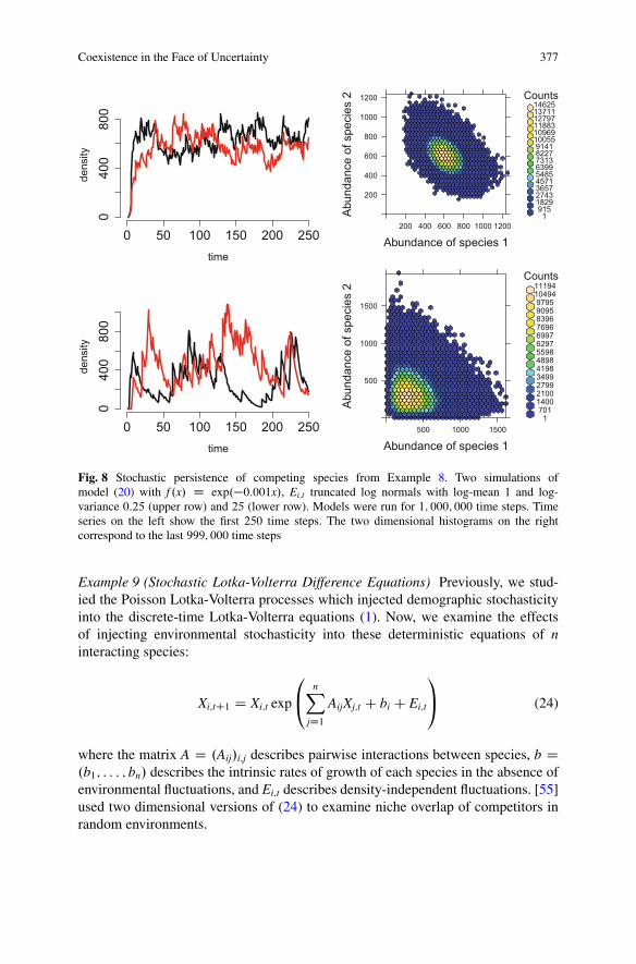
As inequalities (22) and (23) imply inequality (21) for any p1; p2 > 0, inequali-ties (22) and (23) imply stochastic persistence. These inequalities correspond to theclassical mutual invasibility criterion [55]: if each of the species can increase whenrare, the competing species coexist.
To verify whether or not these conditions are satisfied is, in general, a challengingissue. However, [12] developed a formula for the ri.�/ when the competition issymmetric. Namely, s1 D s2 DW s, Et are independent and identically distributed,and E1;t; E2;t are exchangeable i.e. PŒ.E1;t; E2;t/ 2 B� D PŒ.E2;t; E1;t/ 2 B� for anyBorel B � E � E . Before describing Chesson’s formula, lets examine the dynamicsof the deterministic case. Exchangeability and determinism imply there exists a

376 S.J. Schreiber
constant E > 0 such that E1;t D E2;t D E for all t. Hence, the deterministic modelis given by
xi;tC1 D xi;t .Ef .Ex1;t C Ex2;t/ C s/ with i D 1; 2:
As x1;tC1=x2;tC1 D x1;t=x2;t for all t, all radial lines in the positive orthant areinvariant. Provided Ef .0/ C s > 1 (i.e. each species persists in the absence ofcompetition), there exists a line of equilibria connecting the two axes. Regardingthese neutral dynamics, [12] wrote
“Classically, when faced with a deterministic model of this sort ecologists have concludedthat only one species can persist when the likely effects a stochastic environment aretaken into account. The reason for this conclusion is the argument that environmentalperturbations will cause a random walk to take place in which eventually all but one speciesbecomes extinct.”
Dispelling this faulty expectation, [12] derived a formula for the ri.�/. Todescribe this formula, assume inequality (21) holds and � is an ergodic, stationarydistribution supporting species 1. As the Et are independent in time, � can be writtenas a product measure m � � on S � E where � is given by Hypothesis 3.7. Define
h.E1; E2/ DZ
log .E2f .x1E1/ C s/ m.dx/:
[12] showed that
r2.�/ D �1
2E
"Z E2;t
E1;t
Z E2;t
E1;t
@2h
@E1@E2
.E1; E2/dE1dE2
#:
As f is a decreasing function,
@2h
@E1@E2
.E1; E2/ D f 0.x1E1/x1s
.E2f .x1E1/ C s/2< 0
whenever s > 0. Hence, r2.�/ > 0 provided that PŒE1;t > E2;t� > 0 (i.e. there issome variation) and s > 0. As this holds for any ergodic � supporting species 1
and a similar argument yields r1.�/ > 0 for any ergodic � supporting species 2, itfollows that this symmetric version of the model is stochastically persistent (Fig. 8).
The analysis of this model highlights three key ingredients required for environ-mental fluctuations to mediate coexistence. First, there must periods of time suchthat each species has a higher birth rate i.e. E1;t and E2;t vary and are not perfectlycorrelated. Second, year to year survivorship needs to be sufficiently positive (i.e.s > 0 in the model) to ensure species can “store” the gains from one favorable periodto the next favorable period. Finally, the increase in fitness due to good conditionsfor one species is greater in years when those conditions are worse for its competitori.e. @2h
@[email protected]; E2/ < 0. These are the key ingredients of the “storage effect” as
introduced by [14].
Coexistence in the Face of Uncertainty 377
0 50 100 150 200 250
040
080
0
time
dens
ity
Abundance of species 1
Abu
ndan
ce o
f spe
cies
2
200
400
600
800
1000
1200
200 400 600 800 1000 1200
Counts
1915182927433657457154856399731382279141100551096911883127971371114625
0 50 100 150 200 250
040
080
0
time
dens
ity
Abundance of species 1
Abu
ndan
ce o
f spe
cies
2
500
1000
1500
500 1000 1500
Counts
1701
14002100279934994198489855986297699776968396909597951049411194
Fig. 8 Stochastic persistence of competing species from Example 8. Two simulations ofmodel (20) with f .x/ D exp.�0:001x/, Ei;t truncated log normals with log-mean 1 and log-variance 0:25 (upper row) and 25 (lower row). Models were run for 1; 000; 000 time steps. Timeseries on the left show the first 250 time steps. The two dimensional histograms on the rightcorrespond to the last 999; 000 time steps
Example 9 (Stochastic Lotka-Volterra Difference Equations) Previously, we stud-ied the Poisson Lotka-Volterra processes which injected demographic stochasticityinto the discrete-time Lotka-Volterra equations (1). Now, we examine the effectsof injecting environmental stochasticity into these deterministic equations of ninteracting species:
Xi;tC1 D Xi;t exp
0@
nXjD1
AijXj;t C bi C Ei;t
1A (24)
where the matrix A D .Aij/i;j describes pairwise interactions between species, b D.b1; : : : ; bn/ describes the intrinsic rates of growth of each species in the absence ofenvironmental fluctuations, and Ei;t describes density-independent fluctuations. [55]used two dimensional versions of (24) to examine niche overlap of competitors inrandom environments.
378 S.J. Schreiber
The following lemma shows that verifying persistence for these equationsreduces to a linear algebra problem. In particular, this lemma implies that thepermanence criteria developed by [26] extend to these stochastically perturbedLotka-Volterra systems.
Lemma 3.1 Let � be an ergodic stationary distribution for (24) and I � f1; : : : ; kgbe the species supported by � i.e. �.fx 2 S W xi > 0 iff i 2 Ig � E / D 1. Defineˇi D bi C EŒEi;t�. If there exists a unique solution Ox to
Xj2I
Aij Oxj C ˇi D 0 for i 2 I and Oxi D 0 for i … I (25)
then
ri.�/ D(
0 if i 2 IPj2I Aij Oxj C ˇi otherwise.
The following proof of this lemma is nearly identical to the proof given by [50] forthe case Et are independent and identically distributed in time.
Proof Let � and I be as assumed in the statement of the lemma. We have
ri.�/ DXj2I
Aij
Zxj �.dxdE/ C ˇi
for all i. As ri.�/ D 0 for all i 2 I,
0 DXj2I
Aij
Zxj �.dxdE/ C ˇi
for all i 2 I. Since we have assumed there is a unique solution Ox to this system oflinear equations, it follows that
Rxi�.dxdE/ D Oxi for all i and the lemma follows.
utThis lemma implies that verifying the stochastic persistence condition reduces to
finding p1; : : : ; pn > 0 such that
Xi…I
pi
Xj2I
Aij Oxj C ˇi > 0
for every I � f1; : : : ; ng and Ox 2 S0 satisfying equation (25). The next exampleillustrates the utility of this criterion.
Example 10 (Rock-Paper-Scissor Dynamics) The Lotka-Volterra model of rock-paper-scissor dynamics is a prototype for understanding intransitive ecologicaloutcomes [37, 52]. Here, a simple stochastic version of this dynamic is given
Coexistence in the Face of Uncertainty 379
by (24) with X1; X2; X3 corresponding to the densities of the rock, paper, and scissorspopulations, and the matrixes A and b given by
A D �1 C0@
0 �`2 w3
w1 0 �`3
�`1 w2 0
1A and b D
0@
1
1
1
1A
with 1 > wi > 0 and `i > 0. The �`i correspond to a reduction in the per-capitagrowth rate of the population losing against population i, and wi corresponds to theincrease in the per-capita growth rate of the population winning against populationi. Assume that the Ei;t in (24) are compactly supported random variables with zeroexpectation. Under this assumption, ˇi as defined in Lemma 3.1 equal 1.
Our assumptions about A and b imply that in pairwise interactions population 1 isexcluded by population 2, population 2 is excluded by population 3, and population3 is excluded by population 1. Hence, there are only four solutions of (25) that needto be considered: Ox D .0; 0; 0/, Ox D .1; 0; 0/, Ox D .0; 1; 0/, and Ox D .0; 0; 1/. Hence,verifying stochastic persistence reduces to determining whether there exist positivereals p1; p2; p3 such that
p1 C p2 C p3 > 0
p1 0 C p2w1 � p3`1 > 0
�p1`2 C p2 0 C p3w2 > 0
p1w3 � p2`3 C p3 0 > 0
where these equation come from evaluatingP
i piri.�/ at ergodic measures corre-sponding to .0; 0; 0/, .1; 0; 0/, .0; 1; 0/, and .0; 0; 1/. Solving these linear inequali-ties implies that there is the desired choice of pi if and only if w1w2w3 > `1`2`3 i.e.the geometric mean of the fitness payoffs to the winners exceeds the geometric meanof the fitness losses of the losers. Figure 9 illustrates the dynamics of coexistencewhen w1w2w3 > `1`2`3 and exclusion when w1w2w3 < `1`2`3.
4 Parting Thoughts and Future Challenges
The results reviewed here provide some ways to think about species coexistenceor population persistence in the face of uncertainty. In the face of demographicuncertainty, species may coexist for exceptionally long periods of time prior to goingextinct. I discussed how this metastable behavior may be predicted by the existenceof positive attractors for the underlying deterministic dynamics, in which case thetimes to extinction increase exponentially with habitat size. Alternatively, in the face

380 S.J. Schreiber
0 200 400
0.2
0.4
0.6
0.8
time
dens
ities
0 200 400
0.0
0.4
0.8
1.2
time
dens
ities
Fig. 9 Stochastic rock-paper-scissor dynamics (Example 10) with stochastic persistence in theleft hand panel (wi D 0:3 > 0:2 D `i for all i) and stochastic exclusion in the right hand panel(wi D 0:2 < 0:3 D `i for all i)
of environmental stochasticity, species may coexist in the sense of rarely visiting lowdensities. I discussed how this form of stochastic persistence can be identified byexamining species’ per-capita growth rates ri.�/ when rare. Weighted combinationsof these per-capita growth rates can measure to what extent communities move awayextinction as one or more species become rare. Despite this progress, many excitingchallenges lie ahead.
Many demographic processes and environmental conditions vary continuouslyin time and are better represented by continuous time models. For continuous-time Markov chains accounting for demographic stochasticity, [36] proved resultssimilar to Theorems 2.5 and 2.6 discussed here. For stochastic differential equationsof interacting, unstructured populations in fluctuating environments, there existsome results similar to Theorem 3.11 by [6, 50] and [19]. These stochasticdifferential equations, however, fail to account for population structure or correlatedenvironmental fluctuations. One step toward temporally correlated environmentswas recently taken by [4]. They characterized stochastic persistence for continuous-time models of competing species experiencing a finite number of environmentalstates driven by a continuous-time Markov chain. Generalizing these results tohigher dimensional communities and structured populations remains an impor-tant challenge. Another exciting possibility is studying stochastic persistence forcontinuous-time models with stochastic birth or mortality impulses, as oftenobserved in nature.
Biologists often measure continuous traits (e.g. body size or geographical loca-tion of an individual) that have important demographic consequences (e.g. largerindividuals may produce more offspring and be more likely to survive). Unlikemodels accounting for discrete traits as considered here, models with continuoustraits are infinite-dimensional and, consequently, even stochastic counterparts onlyaccounting for demographic stochasticity correspond to Markov chains on uncount-
Coexistence in the Face of Uncertainty 381
able state spaces (see, e.g., [53]). One form of these models, integral projectionmodels (IPMs), have become exceptionally popular in the ecological literature inthe past decade as they interface well with demographic data sets (see, e.g., [43]for a recent discussion). Consequently, there is a need for the development of theinfinite-dimensional counterparts to the results presented here (see [23] for resultsfor structured populations facing uncorrelated, environmental stochasticity).
For both forms of stochasticity, there are few results for demonstrating thatpopulations are “extinction-prone” (e.g. limiting QSDs being supported by theextinction set in Theorem 2.5 or Benaïm et al. [6, Theorems 4.2,5.1] for stochasticdifferential equations). No study of persistence or coexistence is complete withoutunderstanding this complementary outcome. Hopefully, answers to Problems 2and 6 will narrow our gap in understanding these outcomes. Furthermore, evenwhen populations aren’t extinction prone in the aforementioned sense, extinctionis inevitable as all real population are finite. Answers to Problem 3 and theirapplications to specific models could provide new insights about how feedbacksbetween nonlinearities and noise determine the “intrinsic” extinction probabilities,quantities of particular importance for conservation biology.
Finally, there is the elephant in the review: what can one say for modelsaccounting for both forms of stochasticity? At this point, all I have to offer is anatural conjecture which combines the results presented here. Namely, let xtC1 DF.xt; EtC1/ be a random difference equation and fX"
t g">0 be a family of Markovchains satisfying the environmental dependent versions of Hypotheses 2.3 and 2.4e.g. the rate function � in Hypothesis 2.3 depends on E 2 E as well as x; y 2 S .In light of the results presented here, these models lead to the following challengingproblem:
Problem 7 Is it true that stochastic persistence of xtC1 D F.xt; EtC1/ implies theweak* limit points of the QSDS of fX"
t g">0 are supported by SC and �" � 1 �exp.�c="/ for some c > 0?
I believe there should be an affirmative answer to this question. Namely, stochasticpersistence in the face of environmental fluctuations implies long-term, persistent,metastable behavior for communities of interacting populations of finite size, andthe extinction probabilities decay exponentially with community “size.” Hopefully,this review will inspire work to address this problem as well as for the otherchallenges posed here.
Acknowledgements Many thanks to Swati Patel, William Cuello, and two anonymous reviews forproviding extensive comments on an earlier version of this manuscript. This work was supportedin part by US NSF Grant DMS-1313418 to the author.

382 S.J. Schreiber
References
1. P.B. Adler, S.P. Ellner, and J.M. Levine. Coexistence of perennial plants: an embarrassment ofniches. Ecology letters, 13:1019–1029, 2010.
2. L. Arnold. Random dynamical systems. Springer Monographs in Mathematics. Springer-Verlag, Berlin, 1998. ISBN 3-540-63758-3.
3. A.D. Barbour. Quasi-Stationary Distributions in Markov Population Processes. Advances inApplied Probability, 8:296–314, 1976.
4. M. Benaïm and C. Lobry. Lotka Volterra in fluctuating environment or “how good can be bad”.arXiv preprint arXiv:1412.1107, 2014.
5. M. Benaïm and S.J. Schreiber. Persistence of structured populations in random environments.Theoretical Population Biology, 76:19–34, 2009.
6. M. Benaïm, J. Hofbauer, and W. Sandholm. Robust permanence and impermanence for thestochastic replicator dynamics. Journal of Biological Dynamics, 2:180–195, 2008.
7. P. Chesson. Multispecies competition in variable environments. Theoretical Population Biol-ogy, 45(3):227–276, 1994.
8. P. Chesson. General theory of competitive coexistence in spatially-varying environments.Theoretical Population Biology, 58:211–237, 2000.
9. P. Chesson. Mechanisms of maintenance of species diversity. Annual Review of Ecology andSystematics, 31:343–366, 2000. ISSN 00664162.
10. P. L. Chesson. Predator-prey theory and variability. Annu. Rev. Ecol. Syst., 9:323–347, 1978.11. P. L. Chesson. The stabilizing effect of a random environment. J. Math. Biol., 15(1):1–36,
1982.12. P.L. Chesson. Interactions between environment and competition: how environmental fluc-
tuations mediate coexistence and competitive exclusion. Lecture Notes in Biomathematics,77:51–71, 1988.
13. P.L. Chesson and S. Ellner. Invasibility and stochastic boundedness in monotonic competitionmodels. Journal of Mathematical Biology, 27:117–138, 1989.
14. P.L. Chesson and R.R. Warner. Environmental variability promotes coexistence in lotterycompetitive systems. The American Naturalist, 117(6):923, 1981.
15. J.N. Darroch and E. Seneta. On quasi-stationary distributions in absorbing discrete-time finitemarkov chains. Journal of Applied Probability, 2:88–100, 1965.
16. A. Dembo and O. Zeitouni. Large Deviation Techniques and Applications. Applications ofMathematics: Stochastic Modelling and Applied Probability. Springer, 1993.
17. R. Durrett. Probability: Theory and examples. Duxbury Press, Belmont, CA, 1996.18. S.N. Evans, P. Ralph, S.J. Schreiber, and A. Sen. Stochastic growth rates in spatio-temporal
heterogeneous environments. Journal of Mathematical Biology, 66:423–476, 2013.19. S.N. Evans, A Hening, and S.J. Schreiber. Protected polymorphisms and evolutionary stability
of patch-selection strategies in stochastic environments. Journal of Mathematical Biology,71:325–359, 2015.
20. M. Faure and S. J. Schreiber. Quasi-stationary distributions for randomly perturbed dynamicalsystems. Annals of Applied Probability, 24:553–598, 2014.
21. M. I. Freidlin and A. D. Wentzell. Random perturbations of dynamical systems, volume 260 ofGrundlehren der Mathematischen Wissenschaften [Fundamental Principles of MathematicalSciences]. Springer-Verlag, New York, second edition, 1998. ISBN 0-387-98362-7. Translatedfrom the 1979 Russian original by Joseph Szücs.
22. V. Grimm and C. Wissel. The intrinsic mean time to extinction: a unifying approach toanalysing persistence and viability of populations. Oikos, 105:501–511, 2004.
23. D. P. Hardin, P. Takác, and G. F. Webb. Asymptotic properties of a continuous-space discrete-time population model in a random environment. Journal of Mathematical Biology, 26:361–374, 1988a. ISSN 0303-6812.
24. G. Hardin. The tragedy of the commons. Science, 162:1243–1248, 1968.
Coexistence in the Face of Uncertainty 383
25. J. Hofbauer. A general cooperation theorem for hypercycles. Monatshefte für Mathematik,91:233–240, 1981.
26. J. Hofbauer, V. Hutson, and W. Jansen. Coexistence for systems governed by differenceequations of Lotka-Volterra type. Journal of Mathematical Biology, 25:553–570, 1987.
27. G. Högnäs. On the quasi-stationary distribution of a stochastic Ricker model. StochasticProcesses and their Applications, 70:243–263, 1997.
28. G.E. Hutchinson. The paradox of the plankton. The American Naturalist, 95:137–145, 1961.29. P. Jagers. A plea for stochastic population dynamics. Journal of Mathematical Biology,
60:761–764, 2010.30. W. O. Kermack and A. G. McKendrick. A contribution to the mathematical theory of
epidemics. Proceedings of the Royal society of London. Series A, 115:700–721, 1927.31. Y. Kifer. Random perturbations of dynamical systems. Birkhauser, New York, 1988.32. F.C. Klebaner, J. Lazar, and O. Zeitouni. On the quasi-stationary distribution for some
randomly perturbed transformations of an interval. Annals of Applied Probability, 8:300–315,1998. ISSN 1050-5164.
33. O. S. Kozlovski. Axiom A maps are dense in the space of unimodal maps in the Ck topology.Annals of Mathematics, 157:1–43, 2003. ISSN 0003-486X.
34. Thomas G. Kurtz. Approximation of population processes, volume 36 of CBMS-NSF RegionalConference Series in Applied Mathematics. Society for Industrial and Applied Mathematics(SIAM), Philadelphia, Pa., 1981. ISBN 0-89871-169-X.
35. A. J. Lotka. Elements of Physical Biology. Williams and Witkins, Baltimore, 1925.36. B. Marmet. Quasi-stationary distributions for stochastic approximation algorithms with con-
stant step size. arXiv preprint arXiv:1303.7081, 2013.37. R. M. May and W. Leonard. Nonlinear aspects of competition between three species. SIAM
Journal of Applied Mathematics, 29:243–252, 1975.38. J. F. McLaughlin, J. J. Hellmann, C. L. Boggs, and P. R. Ehrlich. Climate change hastens
population extinctions. Proceeding of the National Academy of Sciences USA, 99:6070–6074,2002.
39. S. Méléard and D. Villemonais. Quasi-stationary distributions and population processes.Probability Surveys, 9:340–410, 2012.
40. J.A.J. Metz, T.J. de Jong, and P.G.L. Klinkhamer. What are the advantages of dispersing; apaper by Kuno extended. Oecologia, 57:166–169, 1983.
41. A. J. Nicholson and V. A. Bailey. The balance of animal populations. Proceedings of theZoological Society of London, pages 551–598, 1935.
42. K. Ramanan and O. Zeitouni. The quasi-stationary distribution for small random perturbationsof certain one-dimensional maps. Stochastic Processes and Applications, 84:25–51, 1999.ISSN 0304-4149.
43. M. Rees, D.Z. Childs, and S.P. Ellner. Building integral projection models: a user’s guide.Journal of Animal Ecology, 83:528–545, 2014.
44. G. Roth and S.J. Schreiber. Persistence in fluctuating environments for interacting structuredpopulations. Journal of Mathematical Biology, 68:1267–1317, 2014.
45. D. Ruelle. Analycity properties of the characteristic exponents of random matrix products.Advances in Mathematics, 32:68–80, 1979. ISSN 0001-8708.
46. S. J. Schreiber. Allee effects, chaotic transients, and unexpected extinctions. TheoreticalPopulation Biology, 2003.
47. S. J. Schreiber. Persistence despite perturbations for interacting populations. Journal ofTheoretical Biology, 242:844–52, 2006.
48. S. J. Schreiber. On persistence and extinction of randomly perturbed dynamical systems.Discrete and Continous Dynamical Systems B, 7:457–463, 2007.
49. S. J. Schreiber. Persistence for stochastic difference equations: a mini-review. Journal ofDifference Equations and Applications, 18:1381–1403, 2012.
50. S. J. Schreiber, M. Benaïm, and K. A. S. Atchadé. Persistence in fluctuating environments.Journal of Mathematical Biology, 62:655–683, 2011.

384 S.J. Schreiber
51. S.J. Schreiber. Interactive effects of temporal correlations, spatial heterogeneity and dis-persal on population persistence. Proceedings of the Royal Society B: Biological Sciences,277:1907–1914, 2010.
52. S.J. Schreiber and T.P. Killingback. Cycling in space: Persistence of rock-paper-scissormetacommunities. Theoretical Population Biology, 86:1–11, 2013.
53. S.J. Schreiber and N. Ross. Individual-based integral projection models: The role of size-structure on extinction risk and establishment success. Methods in Ecology and Evolution,in press. URL http://onlinelibrary.wiley.com/doi/10.1111/2041-210X.12537/abstract.
54. W. R. Thompson. La théorie mathématique de l’action des parasites entomophages et le facteurdu hassard. Annales Faculte des Sciences de Marseille, 2:69–89, 1924.
55. M. Turelli. Niche overlap and invasion of competitors in random environments i. modelswithout demographic stochasticity. Theoretical Population Biology, 20:1–56, 1981.
56. V. Volterra. Fluctuations in the abundance of a species considered mathematically. Nature,118:558–560, 1926.