coffee cultivation in a changing climate

COFFEE CULTIVATION IN A CHANGING CLIMATE

BACHELOR PROJECT

1

Hannah ter Steege S3421406 Bachelor Spatial Planning and Design Bachelor Project – Assignment 7, Final version Supervisor: Gunnar Mallon Date: 15th of January, 2021

2

Table of Contents Tables and Figures ..................................................................................................................... 3

1. Summary ............................................................................................................................. 4

2. Introduction ........................................................................................................................ 5

2.1 Background ....................................................................................................................... 5

2.2 Research problem ............................................................................................................. 5

2.3 Structure of thesis ............................................................................................................. 6

3. Theoretical Framework ....................................................................................................... 6

4. Methodology ....................................................................................................................... 8

5. Results ............................................................................................................................... 10

5.1 Locations for coffee cultivation ................................................................................. 10

5.2 Suitability current locations for coffee cultivation ..................................................... 11

5.3 Climate projections and future sustainability ............................................................ 13

5.3.1 The Americas .............................................................................................................14

5.3.2 Africa .........................................................................................................................16

5.3.3 South-East Asia .........................................................................................................19

6. Conclusions ....................................................................................................................... 22

7. Discussion ......................................................................................................................... 23

References ................................................................................................................................ 24

Appendix 1 – Precipitation projections – script ...................................................................... 26

Appendix 2 – Temperature Projections – script ...................................................................... 28

Appendix 3 – Suitability calculations water – script ............................................................... 30

Appendix 4 – Configuration file PCR-GLOBWB model .......................................................... 32

3

Tables and Figures Figure 1 – Conceptual model ..................................................................................................... 8

Figure 2 - Coffee producing countries ...................................................................................... 10

Figure 3 - Legend Suitability coffee cultivation ........................................................................ 11

Figure 4 - Suitability for coffee cultivation in the Americas (2020) .........................................12

Figure 5 - Suitability for coffee cultivation in Africa (2020) .....................................................12

Figure 6 - Suitability for coffee cultivation in South-East Asia (2020) ....................................12

Figure 7 - Legend precipitation projections .............................................................................. 13

Figure 8 - Legend temperature projections .............................................................................. 13

Figure 9 - Precipitation projections for the Americas ...............................................................14

Figure 10 - Temperature projections for the Americas .............................................................14

Figure 11 - Sustainability coffee cultivation RCP 2.6 - The Americas ....................................... 15

Figure 12 - Sustainability coffee cultivation RCP 4.5 - The Americas ....................................... 15

Figure 13 - Sustainability coffee cultivation RCP 6.0 - The Americas ......................................16

Figure 14 - Sustainability coffee cultivation RCP 8.5 ................................................................16

Figure 15 - Precipitation projections for Africa ......................................................................... 17

Figure 16 - Temperature projections for Africa ........................................................................ 17

Figure 17 - Sustainability coffee cultivation RCP 2.6 - Africa .................................................. 18

Figure 18 - Sustainability coffee cultivation RCP 4.5 – Africa ................................................. 18

Figure 19 -Sustainability coffee cultivation RCP 6.0 - Africa ....................................................19

Figure 20 - Sustainability coffee cultivation RCP 8.5 - Africa .................................................19

Figure 21 - Precipitation projections for South-East Asia ....................................................... 20

Figure 22 - Temperature projections for South-East Asia ....................................................... 20

Figure 23 - Sustainability coffee cultivation RCP 2.6 - South-East Asia ..................................21

Figure 24 - Sustainability coffee cultivation RCP 4.5 - South-East Asia..................................21

Figure 25 - Sustainability coffee cultivation RCP 6.0 - South-East Asia ................................. 22

Figure 26 - Sustainability coffee cultivation RCP 8.5 - South-East Asia ................................. 22

Table 1 - Agrometeorological parameters .................................................................................. 9

4

1. Summary About a 100 million people are dependent on the cultivation of coffee (Bunn et al., 2015). The

process of coffee production is one with a very high water footprint. Most of the water

consumed is green water, but as a result of a changing climate it is suspected that there will be

more blue water involved in the process of coffee production (Chapagain and Hoekstra, 2007).

The aim of this research was to investigate how the water footprint of coffee production is

affected by climate change. This is done by answering the research question “How does climate

change influence the water footprint of coffee production and what are the implications for

future coffee production?” By the use of different spatial and statistical analyses, it is

concluded that the areas in which coffee cultivation can be executed will decrease significantly.

Another process is that these areas are moving outside of the current coffee cultivating

countries. The result is that many plantations will suffer from the changing climate, and that

there should be looked into smart methods for coffee cultivation regarding water consumption

and heat stress. This, to ensure the water footprint of coffee cultivation and production is

brought down. Next to this, awareness should be raised about the water footprint of every cup

coffee consumers consume.

5

2. Introduction 2.1 Background A 100 million people are dependent on coffee production (Bunn et al., 2015). The coffee crop

is one of the crops that consumes the most water. It is calculated that for a cup of coffee in the

Netherlands, on average 140 L water is consumed. The largest share of this water is not

consumed in the Netherlands, but in the countries where the coffee is cultivated and produced,

such as Brazil or Mexico (Chapagain and Hoekstra, 2007; Mekonnen and Hoekstra, 2011). A

virtual water flow emerges when in some part of the world, there is a demand for water

consumption somewhere else in that same world. Of the total water consumption, about 16%

is covered by virtual water flows. Of this 16%, about 76% is related to agriculture, and mainly

to crop production (Hoekstra and Mekonnen, 2012). Virtual water trade can either increase or

decrease the global water consumption depending on the efficiency of the trade. This is related

to the fact that countries with a low water productivity often are dependent on countries with

a high water productivity. When there is a high water availability in a country with a high water

productivity, this is efficient. With a low water availability in a country that has a high water

productivity, one might wonder if this can be done more efficiently (Chapagain and Hoekstra,

2008; Hoekstra and Mekonnen, 2012).

2.2 Research problem As stated before, a 100 million people are dependent on coffee and its production process and

the livelihood of these people will very likely be negatively affected by the process of climate

change. Where Arabica coffee already suffers from higher temperatures itself, also coffee pests

will be able to spread quicker. The production of Robusta coffee will be harmed by larger

variations in temperature, and a changing pattern in precipitation will influence the

possibilities for coffee production, as of that there is a lot of water involved in the process of

producing coffee. It is expected that less, or more extreme patterns in, precipitation will ensure

that the blue water footprint increases, where the green decreases. The areas that are suitable

for coffee production will probably change in the coming years, and therefore this research will

look into the effects of climate change on the water footprint of coffee production, and the

implications of this in coffee production in the future. The central question that this research

aims to answer is: “How does climate change influence the water footprint of coffee

production and what are the implications for future coffee production?”

To find an answer to this question, several aspects are investigated. To begin with, a picture of

the locations of current coffee plantations is essential to start with the research. Sub-question

1 (S1) is derived from this: “What are current locations for coffee production?” It is also

interesting to see whether there are, at this moment, locations for coffee productions which are

not sustainable anymore. Therefore, sub-question 2 (S2) is the following: “Which current

locations for coffee production are not suitable for sustainable coffee production?”. Next to

this, sub-question 3 (S3) is relevant for the climate projections: regional climate projections of

the current coffee-producing areas are necessary to be known to make an analysis on the

sustainability of coffee production in the future. Thus, sub-question 3 is: “What are climate

projections for the current coffee-producing areas?” From the first sub-question, a final sub-

question can be constructed (S4): “Which areas are likely to experience a decline in the

sustainability of coffee production in the (near) future?”

The research was focused on the cultivation of the crop, as it isn’t be feasible in the given

amount of time to include other parts of the coffee production process as well. There is looked

into the climatic stressors that indicate whether or not coffee cultivation is sustainable in

certain areas.

6

2.3 Structure of thesis When reading this thesis, one will find a clear structure on the research and its process. In

Chapter 2, a theoretical framework is created to create the basis for the research. Key terms are

explained, and a conceptual model is created to show the connections between the different

key terms. In the end of this chapter, hypotheses are drawn up. Chapter 3 will describe the

methodological approach for this research. It will explain this research had a quantitative

approach, the reasons for this approach, and the process of data collection and analysis.

Chapter 4, the results, will be split up in multiple sub-chapters, each finding the main results

for the different sub-questions and the main question that are composed in the Research

Problem per area. In Chapter 5, conclusions will be drawn, and in Chapter 7 there will be a

discussion on the shortcomings of the research, the findings are compared with existing

literature, and recommendations for further research are given.

3. Theoretical Framework The water footprint is a tool that can be used to quantify the amount of fresh water consumed

in the production of a good. For an even better insight, a subdivision is created with three main

components: the green, blue and grey water footprint. The green and the blue water footprint

are related directly to freshwater consumption, where the grey water footprint is related to

pollution of the water as a result of production processes. The green water footprint is the

amount of rainwater consumed (or evaporated) in a production process. The blue water

footprint is the amount of ground and surface water that is consumed (evaporated) in the

production process. The blue water footprint tends to be higher in areas where there is a higher

water scarcity. This can be related to the fact that in those areas, there is less green water

available for consumption. The grey water footprint is the amount of fresh water that is needed

to bring down the concentrations of pollutants in waste waters to acceptable levels. The use of

fertilizers increases the grey water footprint, as it causes pollution of the ground and waste

water (Mekonnen and Hoekstra, 2011; Hoekstra et al., 2012).

Most of the water that is consumed for coffee production is rain water, or green water.

However, after the harvesting of the berries, there are two production processes: a dry and a

wet one. In the wet production process, the grey and the blue water footprint of coffee

production increases significantly (Chapagain and Hoekstra, 2007). It is visible that in areas

where the green water supply is smaller, blue water consumption increases significantly. In

areas with a lower water productivity, the result of less precipitation is that ground and surface

water becomes necessary for production. In the largest part of the cases, groundwater aquifers

are already being overexploited by humans, and thus it is necessary to find ways in producing

for which the blue water footprint is lower (Mekonnen and Hoekstra, 2011; Gleeson et al.,

2012). The blue water footprint might be decreased by investing in new technology in for

example storing green water, or using smart methods in irrigation (Hoekstra and Chapagain,

2007). The same article suggests to shift production processes from areas where water scarcity

is a major problem to areas where this problem is less prominent. Economic welfare and water

consumption are related: water consumption tends to increase with an increasing economic

welfare. An increase of demand for goods and thus an increase of virtual water flows is a cause

for this (Hoekstra and Chapagain, 2007).

A virtual water flow emerges when demand for certain goods in one part of the world influences

the water consumption in another part of the world. It turns out that as a result of the

globalization of trade, the ‘real’ water flows in a region are often dependent on the demand for

goods somewhere else in the world (Chapagain and Hoekstra, 2008; Carr et al., 2013). A

concept closely related to this is the virtual water content that is described by Chapagain and

Hoekstra (2007). The virtual water content seems to be more or less the same as the water

footprint of a product, but it looks into the different phases of the production process. It thus

7

indicates the amount of water necessary per unit of the good in a certain phase of the

production process.

As mentioned before, the water footprint is impacted by economic growth, but also by

population growth, production/trade patterns, consumption patterns and technological

development (Ercin and Hoekstra, 2014). The availability of the same water is also determined

for a large part by human factors. Climatic factors of course play an important role as well, but

climate change is amplified by humans (Steinfeld et al., 2020). Contrary to the positive relation

between economic welfare and water consumption, is the relation between economic welfare

and the negative effects of climate change. The largest effects of climate change are often found

in less wealthy countries. Water related problems belong to this category: water security

problems often tend to impact both ecological and economic activities at the same time. The

most vulnerable areas are the areas that have fewer economic means to invest in a higher water

security, and wealthy countries can get away with symptom treatments regarding water

security. This causes that existing problems aren’t solved fundamentally (Vörösmarty et al.,

2010).

Not only water is one of the climatic stressors that has a high influence on the production of

coffee, temperature also is of high influence (Gay et al., 2006). The coffee plants itself are

dependent on the height of the temperature, and fluctuations in temperature, but also the

different coffee pests depend on the temperature. For example the most frequent occurring

pest for coffee, the coffee berry borer (Hypothenemus hampei), appears to do well in warmer

climates. When this pest will be able to increase its geographical spread as a result of a warming

climate, mainly the production of the Arabica coffee (coffea arabica or c. arabica) will be heavily

impacted (Jaramillo et al., 2011).

In different parts of the world, different methods for coffee cultivation are found. In regions

such as Brazil, the largest parts of the coffee plantations are in full sunlight. Advantages of this

are a higher production per plant, and there are more possibilities for mechanization. The

downside of this is a higher risk for hydric stress, heat stress, and a higher vulnerability to for

example a high variability in temperature. In other parts of the world, such as Central America

and in Indonesia, there are shaded plantations, often in the form of agroforest systems (Vieira,

2008; Siles et al., 2010). An agroforest system is a method for agriculture in which coffee is

grown under trees. Trees provide for shade, and can function as a temperature buffer for coffee,

so heat stress will be less problematic, and the evaporation from the coffee plants will be lower.

The water consumption of the agroforest systems is however higher than in monoculture

systems (Lin, 2007; Siles et al., 2010)

Agroforestry systems have various advantages for the production and growth of coffee (Siles et

al., 2010). For example, as the trees provide shade for the coffee, some sort of a temperature

buffer is created, and this reduces the stress caused by large temperature variations. This is

only useful when there is an urgent need for shade, such as in locations with a warm and dry

climate and the different coffee species would experience different effects. For example,

Arabica coffee is more vulnerable to higher temperatures, where Robusta coffee will suffer

more from a higher variability in temperatures (Beer et al., 1998; Bunn et al., 2015). The

average life span of a coffee plantation is around 30 years, and thus, most coffee plantations

will suffer from climate change. In the near future, the suitability for coffee production of areas

such as Mexico and the Southeast of Africa might decrease significantly (Bunn et al., 2015).

The water footprint of a single catchment area is determined by many factors. These factors

are indicated in the Water Footprint Assessment Manual that was developed by Hoekstra et

al. (2012). In Figure 1, figure 3.1 of the Water Footprint Assessment Manual is simplified and

adjusted to the needs of this research. This conceptual model serves as a basis for calculating

the water footprint. The factors indicated in the model should be taken into account when a

8

model is developed that determines the change in water footprint of coffee production. The

sum of the water footprints of every single step in the production process is the total water

footprint of the production process. The sum of the water footprints of all production processes

in an area is the water footprint of a geographical delineated area (Hoekstra et al., 2012). The

water footprint of a product is expressed as water volume per unit of the product. As mass is

best applicable for the case of coffee, the water footprint will be given as water volume per unit

of mass. In this research, the specific water footprint of coffee for different areas is modelled.

Figure 1 – Conceptual model

4. Methodology In the research, there is chosen for a global, quantitative approach. An analysis of secondary

data is executed. Most variables used in the research are ratio variables, which enabled for

many numerical and spatial analyses. The data on de coffee production provided for a basis

when starting the spatial analyses. Spatial locations can be seen as numerical values: every

point on the earth has been assigned a coordinate. Thus, the coffee producing locations served

as a framework to start the rest of the analyses.

To answer sub-question 1, “What are current locations for coffee production?” the data

provided by the International Coffee Organization (ICO) gives an overview of the current coffee

producing countries. The ICO provides data on coffee production, and this data is openly

accessible. The dataset begins in the year 1990. For the research, mainly recent coffee

production is necessary. The dataset only contains data on all coffee exporting countries, and

will thus not include all coffee producing countries. However, it contains data on most

countries, and these will be the countries that produce most coffee. Therefore, this dataset is

deemed sufficient to provide for a rough picture on where coffee is being produced. For the

research, it is expected to cover enough of the current coffee producing areas to be able to do

analyses. The coffee producing countries in itself are nominal variables, and those served as a

basis for spatial analyses, as are made before in courses such as Geographical Information

Systems, and Environment and Engineering. By using GIS-software, in this case a combination

of ArcGIS Pro and QGIS, the coffee producing countries are visualized on a map. This was as a

basis to be able to use the results of research questions 2, 3, and 4 and translate this to a useful

whole.

9

For sub-question 2, several aspects are taken into account. To answer the question in which

parts of the world coffee cultivation is already losing its sustainability, a spatial analysis was

done by the use of QGIS. The different components precipitation, temperature, evaporation

and frost probability were used to execute a raster calculation which shows the suitability of

the current coffee producing areas. The regional data on temperature and precipitation

projections are provided by the IPCC. The different climate scenarios that they have provided,

are available for use as ArcGIS Feature Services through the portal of ArcGIS online. Thus, the

shapefiles are provided by the IPCC, via ESRI. As the IPCC is the authority regarding climate

change, and ESRI is one of the main authorities regarding Geographical Information Systems,

the data provided is judged to be of a trustworthy quality. There is a chance that the data has

lost some of its quality in the process of converting the IPCC data to shapefiles, but this would

happen as well when executing this task as part of the research. As there is limited time, there

is chosen to use this data. The PCR-GLOBWB model that is developed by the University of

Utrecht is perfectly suitable to provide for maps regarding evaporation. The raster data is

provided on a level of detail of 30x30 arcmin (Sutanudjaja et al., 2018). See Appendix 4 for the

configuration file that was used for running this model.

As a more often used method is to use the model by Sutanudjaja et al. (2018), and it is an

internationally acknowledged model, it is argued that this model, and the data provided

together with the model, are suitable for this research. To finally answer the question, the

agrometeorological parameters mentioned in Table 1 are found to be necessary for coffee

production, and thus a division can be made based on these parameters (Zullo et al., 2011).

For all spatial analyses, raster data was used. This data was all converted to be the same raster

format. The files are in a GeoTIFF format, and the all the raster files have, or are converted to

a raster with, the following characteristics:

CRS = EPSG:4326 – WGS84

Range = X [-180,180], Y [-90,90]

Columns: 720

Rows = 360

Cell size X = 0,5 Cell size Y = 0,5

Table 1 - Agrometeorological parameters

Climatic risk Agrometeorological parameter Annual mean temperature

Annual water deficit Frost probability

Low risks (no restrictions)

≥ 18 𝑎𝑛𝑑 ≤ 22 ≥ 0 𝑎𝑛𝑑 ≤ 100 𝑚𝑚 ≤ 25%

Risk of high temperatures

≥ 22 𝑎𝑛𝑑 ≤ 23 ≥ 0 𝑎𝑛𝑑 ≤ 100 𝑚𝑚 ≤ 25%

Risk of frosts ≥ 18 𝑎𝑛𝑑 ≤ 22 ≥ 0 𝑎𝑛𝑑 ≤ 100 𝑚𝑚 > 25% High risks ≤ 18 𝑎𝑛𝑑 ≥ 23 ≥ 150 𝑚𝑚 > 25%

To answer sub-question 3, ‘what are climate projections for the current coffee producing

areas?’ the different projections as provided by the IPCC were used. These are accessible as

ESRI Feature services through the ArcGIS Online portal. To use this data for further analysis,

it should be in the same format as the climatic data calculated by the PCR-GLOBWB model.

Therefore, there is chosen for the earlier mentioned characteristics for the datasets. As the

PCR-GLOBWB model provides for mesh layers on a resolution of 30x30 arcmin, the resolution

10

of the raster layers concerning temperature and precipitation provided by the WorldClim data

should be of the same resolution of 30x30 arcmin (Fick and Hijmans, 2017). Therefore, those

datasets that were not in this resolution yet, were converted to another.

By the combination of the data of sub-questions 2 and 3, sub-question 4 could be answered:

“Which areas are likely to experience a decline in the sustainability of coffee production in the

(near) future?” By using the raster calculation tools in QGIS, several scripts were written to

calculate which areas will be losing their sustainability in for coffee production in the (near)

future (Appendix 1-3). The different climate scenarios provided by the IPCC all give different

outcomes, and thus as a final step, the way in which an area is affected by the climate change

was calculated per climate scenario.

5. Results The results for the different research questions are given and described in this chapter. Per

sub-question, one sub-chapter is given, and at the end of the chapter, the results for the main

research question are provided. For sub-question 3 and 4, a regional approach is used to

structure the results section: it makes more sense to bundle the results per area, than per sub-

question here.

5.1 Locations for coffee cultivation Sub-question 1, “What are current locations for coffee cultivation?”, is answered by an

analysis of the data provided by the International Coffee Organization (ICO). At this moment,

there are according to the data provided by the ICO 56 countries that export and produce

coffee. Of these countries, the largest part produces both the Arabica and the Robusta berry

Figure 2Fout! Verwijzingsbron niet gevonden.. Of the total coffee consumption, about

70% is Arabica coffee (Vieira, 2008; Magrach and Ghazoul, 2015). The Arabica berry has a

higher market value, and grows better in milder climates, such as found on higher altitudes.

The Robusta however, is better weaponed against hydric deficit, but it is more susceptible to

for example the earlier mentioned berry borer. Fout! Verwijzingsbron niet

gevonden.Fout! Verwijzingsbron niet gevonden. gives an overview of the coffee

producing and exporting countries. It is visible that coffee production mainly takes place in

tropical areas around the equator (Vieira, 2008). This is consistent with the fact that for coffee

production, an ideal annual average temperature lies between 18 and 22 °C (Zullo et al., 2011).

11

Figure 2 - Coffee producing countries

The approach to for example shade management varies between the different coffee producing

regions: in Brazil for example, coffee plantations are in full sun, whereas in Central America

and Asia the largest part of the coffee plantations are shaded. Both have advantages and

disadvantages: the plantations in full sunlight have a higher productivity per plant/area, but

these plantations are more vulnerable to hydric stress and pests such as the berry borer. The

shaded plantations have a lower productivity, but are less vulnerable to pests and hydric stress.

Also, there is less environmental disturbance, and the need for advanced technology is smaller.

Agroforestry systems, or shaded systems seems to be more able to prevent for extremes in the

microclimates that occur in coffee plantations (Beer et al., 1998; Moguel and Toledo, 1999; Lin,

2007; Vieira, 2008; Aerts et al., 2017).

5.2 Suitability current locations for coffee cultivation To find an answer to the second sub-question, “Which current locations for coffee production

are not suitable for sustainable coffee production?”, it is necessary to know that there are three

main factors contributing to the suitability of a location for coffee cultivation. These are

temperature, frost probability, and the availability of water. These factors are called

agrometeorological parameters. For the production of Arabica coffee, the ideal annual mean

temperature is found between 18°C and 22°C. For crop production, an annual mean

temperature of 23°C can be seen as the maximum, but in this case, yields will be less. The frost

probability should be below 25%. The annual water deficit should be less than 100 mm (Zullo

et al., 2011). When the annual evapotranspiration exceeds the annual rainfall, blue water will

need to be used for coffee production. In this research, there is a main focus on the temperature

and the availability of water. As visible in Figure 4, 5 and 6, of the areas in which coffee is

cultivated, only small parts score sufficient on both temperature and the availability of water.

The parts of the maps that are coloured green, are regions in which the cultivation of coffee can

be seen as sustainable. The yellow parts indicate a temperature which is on average slightly too

high, but not too high for the coffee cultivation. The orange parts score sufficient regarding

temperature, but in these areas, there are issues concerning water consumption: where

evapotranspiration exceeds numbers of precipitation, blue water is needed for agriculture.

Figure 3 shows the legend for all suitability maps.

12

Figure 3 - Legend Suitability coffee cultivation

Figure 4 - Suitability for coffee cultivation in the Americas (2020)

Figure 5 - Suitability for coffee cultivation in Africa (2020)

13

Figure 6 - Suitability for coffee cultivation in South-East Asia (2020)

5.3 Climate projections and future sustainability For the answer on sub-question 3, “what are climate projections for the current coffee-

producing areas?” the different climate projections as provided by the IPCC are used. The

different climate projections by the IPCC are found as ArcGIS feature services, provided by

ESRI. The different scenarios that are used for the analysis are RCP 2.6, RCP 4.5, RCP 6.0 and

RCP 8.5. The scenarios contain data on both temperature and precipitation. This data is used

for answering sub-question 4: “Which areas are likely to experience a decline in the

sustainability of coffee production in the (near) future?” In the next chapter, there is made a

subdivision per area and per climate projection. A short discussion will follow on temperature

and precipitation, and this is followed by a discussion on the effects on the sustainability of

coffee production. The legends on all temperature and precipitation maps are given below in

Figure 7 and 8.

Figure 7 - Legend precipitation projections Figure 8 - Legend temperature projections

14

5.3.1 The Americas

Figure 9 - Precipitation projections for the Americas

Figure 10 - Temperature projections for the Americas

RCP 2.6

When looking at climate scenario RCP2.6, different elements are visible. One of these is that

there will be a small increase in rainfall in the south of Brazil and along the west coast of South-

America (Figure 9). Large parts of Mexico and Brazil will experience no difference, or a

decrease in precipitation. Next to this, the whole of this area will see a slight increase in

temperature, as visible in Figure 10.

The effects of the climate projections on the sustainability of coffee cultivation for the Americas

are visualized in Figure 1111. The first thing is that there seems to be a decrease in areas that

have the highest score concerning sustainability in the Americas. Where an increase in rainfall

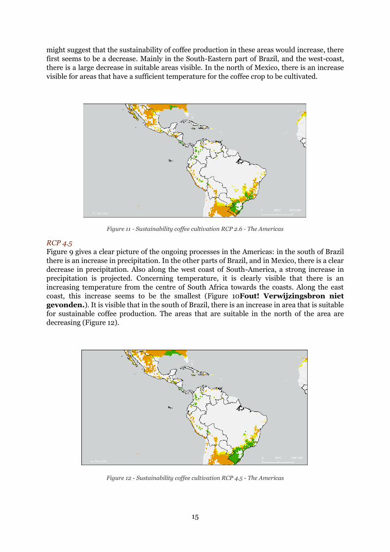
15

might suggest that the sustainability of coffee production in these areas would increase, there

first seems to be a decrease. Mainly in the South-Eastern part of Brazil, and the west-coast,

there is a large decrease in suitable areas visible. In the north of Mexico, there is an increase

visible for areas that have a sufficient temperature for the coffee crop to be cultivated.

Figure 11 - Sustainability coffee cultivation RCP 2.6 - The Americas

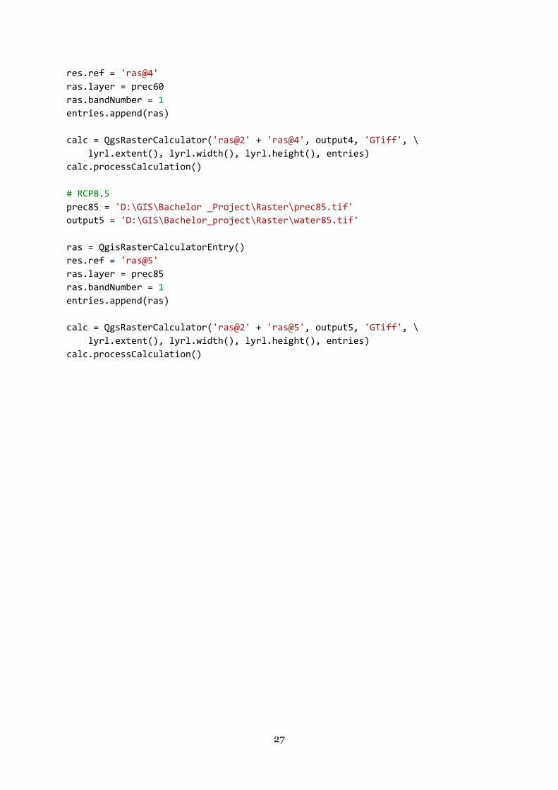
RCP 4.5

Figure 9 gives a clear picture of the ongoing processes in the Americas: in the south of Brazil

there is an increase in precipitation. In the other parts of Brazil, and in Mexico, there is a clear

decrease in precipitation. Also along the west coast of South-America, a strong increase in

precipitation is projected. Concerning temperature, it is clearly visible that there is an

increasing temperature from the centre of South Africa towards the coasts. Along the east

coast, this increase seems to be the smallest (Figure 10Fout! Verwijzingsbron niet

gevonden.). It is visible that in the south of Brazil, there is an increase in area that is suitable

for sustainable coffee production. The areas that are suitable in the north of the area are

decreasing (Figure 12).


16

RCP 6.0

In climate scenario RCP 6.0, it is still clearly visible that the area in which coffee can be

cultivated in a sustainable manner increases in the south of Brazil (Figure 13). That this process

doesn’t occur along the west coast of South America might be caused by the fact that here,

there is not only an increase of precipitation, but also a stronger increase of temperature than

along the east coast (Figure 9, Figure 10). A difference compared towards RCP 4.5 is that in

RCP 6.0 the increase in precipitation is mostly visible in the north east of Brazil, instead of the

south.


RCP 8.5

For climate scenario RCP 8.5, there is a strong increase in temperature projected (Figure

10)Fout! Verwijzingsbron niet gevonden.. Next to this, large parts of Brazil, Mexico and

Venezuela will experience a significant decrease in rainfall (Figure 9). This causes that there

are areas that were suitable for coffee cultivation, tend to become less suitable. The total area

that is suitable for coffee production will decrease, as visible in Figure 14.

Figure 14 - Sustainability coffee cultivation RCP 8.5

5.3.2 Africa The climate projections for Africa cause that there is little variation in the outcomes of the

calculations. Therefore, the results per climate projection are not discussed separately. The

different climate projections on precipitation and temperature are visualized in Figure 15 and

16 respectively.

17

Figure 15 - Precipitation projections for Africa

Figure 16 - Temperature projections for Africa

What follows, is Figure 17Figure 17 that indicates the sustainability of coffee production in

Africa when following climate scenario RCP 2.6. In this area, mainly in south-eastern Africa, it

is already clearly visible what the influence of increasing temperatures (Figure 16), and

increasing drought is on the suitability of this area for coffee production (Figure 15). Where at

the starting point in 2020 there are areas that are noted as areas in which coffee can be

18

cultivated in a sustainable manner, these areas rapidly decrease as a result of a changing

climate.

Figure 17 - Sustainability coffee cultivation RCP 2.6 - Africa

Compared to RCP 2.6, RCP 4.5 brings little surprising elements. The largest parts of the area

will experience more drought (Figure 15), higher temperatures (Figure 15) and less area that

might be suitable for sustainable coffee cultivation (Figure 18).

Figure 18 - Sustainability coffee cultivation RCP 4.5 – Africa

When looking at the other climate scenarios and its possible outcomes, one clear trend is

visible: temperature increases, precipitation decreases, and the area that is suitable for

sustainable coffee cultivation decreases dramatically. This is visualized in Figure 19 and Figure

20 below.

19

Figure 19 -Sustainability coffee cultivation RCP 6.0 - Africa

Figure 20 - Sustainability coffee cultivation RCP 8.5 - Africa

5.3.3 South-East Asia South-East Asia shows a slightly different pattern than Africa and the Americas. Again,

temperature increases in the whole of the area for all climate scenarios (Figure 22). However,

in this area, there are large differences visible in terms of precipitation. In nearly the whole

region, the amount of precipitation will increase as a result of climate change. The only

exceptions for this are found in the north of India, and Java. Only Java shows a significant

decrease in precipitation (Figure 21). 2

20

Figure 21 - Precipitation projections for South-East Asia

Figure 22 - Temperature projections for South-East Asia

The initial change in surface that is suitable for sustainable coffee production seems to decrease

when following climate projection RCP 2.6 (Figure 23) . However, when looking at the other

climate scenarios 4.5 to 8.5, another pattern is visible (Figure 24-26). The area that would be

suitable for sustainable coffee production is found to be increasing. This area is however

shifting to the north. The result is that the areas that are suitable for sustainable coffee

cultivation will be moving outside of the current coffee producing countries.

21

Figure 23 - Sustainability coffee cultivation RCP 2.6 - South-East Asia


22



6. Conclusions To answer the main research question, “How does climate change influence the water

footprint of coffee production and what are the implications for future coffee production?”

the different sub-questions all have been answered. The most obvious conclusion that can be

drawn from this research is that the topic of sustainable coffee production will be one that

becomes more and more relevant in the coming years. As was discovered during the analyses,

clear differences are found in between the regions in which at this moment coffee is cultivated.

Compared to the amount of countries that produce and export coffee, the area that is suitable

for sustainable coffee production is very small, as results from sub-questions 1 and 2. This area

is very likely to decrease in the near future, as for all climate scenarios, a significant decrease

of this area is also visible. Few areas will experience an increase for the suitability of sustainable

coffee production, and these areas will most probably be moving outside of the current areas

of where coffee cultivation takes place.

23

7. Discussion The research into the sustainability of coffee cultivation has its downsides and weak points. To

start off, different problems occurred when working with the PCR-GLOBWB Model, which

caused that there was a need to search for a different approach on the spatial analysis. The

different datasets all were of different formats, and thus needed to be converted to the same

format. A loss of data is here unavoidable. Furthermore, there are many more variables

determining the suitability of an area than only temperature and water availability. However,

due to the scope of this research, there is chosen to make an analysis based on these criteria. A

difference that is found when comparing this research to for example that of Bunn et al. (2015)

is the fact that the area that is ideal for coffee production is larger in the research of Bunn et al.

(2015). This might be caused by the fact that the temperature range that is used by Bunn et al.

(2015) differs from the temperature range used in this research. The research by Bunn et al.

(2015) uses slightly different criteria, as it for example uses more climatic variables.

Nevertheless, a comparable trend is visible. This is in accordance with the more general trend

in literature regarding coffee cultivation in a changing climate. The general trend in literature

regarding the impact of climate change on coffee cultivation is that a large impact is expected

for the coffee cultivation (Gay et al., 2006; Schroth et al., 2009; Jaramillo et al., 2011; Waha

et al., 2013; Craparo et al., 2015). Those involved in the process of coffee cultivation, will most

likely suffer a lot from the expected climate change. This will not only be on the scale of one

plantation, but also on the scale of a country, and thus the effects will be visible on a global

scale (Craparo et al., 2015).

The lifespan of a coffee plantation is about 30 years, and major geographical shifts regarding

the sustainability of locations for coffee cultivation are expected. This is strengthened by the

fact that also Bunn et al. (2015) find a decreasing area that is suitable for the Arabica coffee,

and a shifting area for the Robusta coffee. This will effect in plantation owners losing their

plantations as yields go down, or there is too much irrigation needed for the process of

cultivation to be economically feasible. There is an urge to investigate what implications are

for the different systems for coffee cultivation. Earlier was the distinction between agroforestry

and full-sun plantations made. The different systems, combined with different political and

economic situations and choices will see different effects of the climate change.

To be able to make a better analysis, and to draw more accurate conclusions, it will be necessary

to have a more extensive investigation. In this investigation, there should also be looked into

the differences between Arabica and Robusta coffee, and the irrigation needs per plantation or

region. Future evapotranspiration should be estimated using more complex models and data.

As the water footprint of coffee cultivation is high, it is wise to look into methods which

decrease the water footprint of coffee cultivation: it is advised to investigate methods to store

green water to be prepared for a fluctuating precipitation pattern. It would be wise to look into

smart methods of irrigation, in which less water would be used. When this is successful, the

many persons who are dependent on the production and cultivation of coffee would be helped.

24

References Aerts, R. et al. (2017) ‘Conserving wild Arabica coffee: Emerging threats and opportunities’, Agriculture, Ecosystems and Environment. Elsevier B.V., 237, pp. 75–79. doi: 10.1016/j.agee.2016.12.023.

Beer, J. et al. (1998) ‘Shade management in coffee and cacao plantations’, pp. 139–164. doi: 10.1007/978-94-015-9008-2_6.

Bunn, C. et al. (2015) ‘A bitter cup: climate change profile of global production of Arabica and Robusta coffee’, Climatic Change, 129(1–2), pp. 89–101. doi: 10.1007/s10584-014-1306-x.

Carr, J. A. et al. (2013) ‘Recent History and Geography of Virtual Water Trade’, PLoS ONE, 8(2), pp. 1–10. doi: 10.1371/journal.pone.0055825.

Chapagain, A. K. and Hoekstra, A. Y. (2007) ‘The water footprint of coffee and tea consumption in the Netherlands’, Ecological Economics, 64(1), pp. 109–118. doi: 10.1016/j.ecolecon.2007.02.022.

Chapagain, A. K. and Hoekstra, A. Y. (2008) ‘The global component of freshwater demand and supply: An assessment of virtual water flows between nations as a result of trade in agricultural and industrial products’, Water International, 33(1), pp. 19–32. doi: 10.1080/02508060801927812.

Craparo, A. C. W. et al. (2015) ‘Coffea arabica yields decline in Tanzania due to climate change: Global implications’, Agricultural and Forest Meteorology, 207, pp. 1–10. doi: 10.1016/j.agrformet.2015.03.005.

Ercin, A. E. and Hoekstra, A. Y. (2014) ‘Water footprint scenarios for 2050: A global analysis’, Environment International. Elsevier Ltd, 64, pp. 71–82. doi: 10.1016/j.envint.2013.11.019.

Gay, C. et al. (2006) ‘Potential impacts of climate change on agriculture: A case of study of coffee production in Veracruz, Mexico’, Climatic Change, 79(3–4), pp. 259–288. doi: 10.1007/s10584-006-9066-x.

Gleeson, T. et al. (2012) ‘Water balance of global aquifers revealed by groundwater footprint’, Nature, 488(7410), pp. 197–200. doi: 10.1038/nature11295.

Hoekstra, A. Y. et al. (2012) ‘The Water Footprint Assessment Manual’, The Water Footprint Assessment Manual. doi: 10.4324/9781849775526.

Hoekstra, A. Y. and Chapagain, A. K. (2007) ‘Water footprints of nations: Water use by people as a function of their consumption pattern’, Water Resources Management, 21(1), pp. 35–48. doi: 10.1007/s11269-006-9039-x.

Hoekstra, A. Y. and Mekonnen, M. M. (2012) ‘The water footprint of humanity’, Proceedings of the National Academy of Sciences of the United States of America, 109(9), pp. 3232–3237. doi: 10.1073/pnas.1109936109.

Jaramillo, J. et al. (2011) ‘Some like it hot: The influence and implications of climate change on coffee berry borer (Hypothenemus hampei) and coffee production in East Africa’, PLoS ONE, 6(9). doi: 10.1371/journal.pone.0024528.

Lin, B. B. (2007) ‘Agroforestry management as an adaptive strategy against potential microclimate extremes in coffee agriculture’, Agricultural and Forest Meteorology, 144(1–2), pp. 85–94. doi: 10.1016/j.agrformet.2006.12.009.

Magrach, A. and Ghazoul, J. (2015) ‘Climate and pest-driven geographic shifts in global coffee production: Implications for forest cover, biodiversity and carbon storage’, PLoS ONE, 10(7), pp. 1–15. doi: 10.1371/journal.pone.0133071.

Mekonnen, M. M. and Hoekstra, A. Y. (2011) ‘The green, blue and grey water footprint of

25

crops and derived crop products’, Hydrology and Earth System Sciences, 15(5), pp. 1577–1600. doi: 10.5194/hess-15-1577-2011.

Moguel, P. and Toledo, V. M. (1999) ‘Biodiversity conservation in traditional coffee systems of Mexico’, Conservation Biology, 13(1), pp. 11–21. doi: 10.1046/j.1523-1739.1999.97153.x.

Schroth, G. et al. (2009) ‘Towards a climate change adaptation strategy for coffee communities and ecosystems in the Sierra Madre de Chiapas, Mexico’, Mitigation and Adaptation Strategies for Global Change, 14(7), pp. 605–625. doi: 10.1007/s11027-009-9186-5.

Siles, P. et al. (2010) ‘Rainfall partitioning into throughfall, stemflow and interception loss in a coffee (Coffea arabica L.) monoculture compared to an agroforestry system with Inga densiflora’, Journal of Hydrology. Elsevier B.V., 395(1–2), pp. 39–48. doi: 10.1016/j.jhydrol.2010.10.005.

Steinfeld, C. M. M. et al. (2020) ‘The human dimension of water availability: Influence of management rules on water supply for irrigated agriculture and the environment’, Journal of Hydrology. Elsevier, 588(April), p. 125009. doi: 10.1016/j.jhydrol.2020.125009.

Sutanudjaja, E. H. et al. (2018) ‘PCR-GLOBWB 2: A 5 arcmin global hydrological and water resources model’, Geoscientific Model Development, 11(6), pp. 2429–2453. doi: 10.5194/gmd-11-2429-2018.

Vieira, H. D. (2008) ‘Coffee: The Plant and its Cultivation’, in Souza, R. M. (ed.) Plant-Parasitic Nematodes of Coffee. 1st edn. Campos dos Goytacazes (RJ): Springer, pp. 3–18. doi: 10.1007/978-1-4020-8720-2_8.

Vörösmarty, C. J. et al. (2010) ‘Global threats to human water security and river biodiversity’, Nature, 467(7315), pp. 555–561. doi: 10.1038/nature09440.

Waha, K. et al. (2013) ‘Adaptation to climate change through the choice of cropping system and sowing date in sub-Saharan Africa’, Global Environmental Change, 23(1), pp. 130–143. doi: 10.1016/j.gloenvcha.2012.11.001.

Zullo, J. et al. (2011) ‘Potential for growing Arabica coffee in the extreme south of Brazil in a warmer world’, Climatic Change, 109(3–4), pp. 535–548. doi: 10.1007/s10584-011-0058-0.

26

Appendix 1 – Precipitation projections – script The steps are all executed separately.

# precipitation projections

# RCP2.6

prec26 = 'D:\GIS\Bachelor _Project\Raster\prec26.tif'

output = 'D:\GIS\Bachelor_project\Raster\water26.tif'

entries = []

ras = QgisRasterCalculatorEntry()

res.ref = 'ras@1'

ras.layer = prec26

ras.bandNumber = 1

entries.append(ras)

# annual precipitation

bio12 = 'D:\GIS\Bachelor_Project\Data\Rasters\Precipitation.tif'

output2= 'D:\GIS\Bachelor_Project\Data\Rasters\Precipitation2.tif'


res.ref = 'ras@2'

ras.layer = bio12

ras.bandNumber = 1

entries.append(ras)

calc = QgsRasterCalculator('ras@1' + 'ras@2' , output, 'GTiff', \

lyrl.extent (), lyrl.width(), lyrl.height(), entries)

calc.processCalculation()

# RCP4.5


output3 = 'D:\GIS\Bachelor_project\Raster\water45.tif'


res.ref = 'ras@3'

ras.layer = prec45

ras.bandNumber = 1

entries.append(ras)

calc = QgsRasterCalculator('ras@2'+ 'ras@3', output3, 'GTiff', \

lyrl.extent(), lyrl.width(), lyrl.height(), entries)


# RCP6.0




27

res.ref = 'ras@4'

ras.layer = prec60

ras.bandNumber = 1

entries.append(ras)

calc = QgsRasterCalculator('ras@2' + 'ras@4', output4, 'GTiff', \



# RCP8.5




res.ref = 'ras@5'

ras.layer = prec85

ras.bandNumber = 1

entries.append(ras)




28

Appendix 2 – Temperature Projections – script The steps are all executed separately.

# temperature projections

# RCP2.6

temp26 = 'D:\GIS\Bachelor _Project\Raster\temp26.tif'

output = 'D:\GIS\Bachelor_project\Raster\tottemp26.tif'

entries = []


res.ref = 'ras@1'

ras.layer = temp26

ras.bandNumber = 1

entries.append(ras)

# annual temperature

bio1 = 'D:\GIS\Bachelor_Project\Data\Rasters\temperature.tif'

output2 = 'D:\GIS\Bachelor_Project\Data\Rasters\temperature2.tif'


res.ref = 'ras@2'

ras.layer = bio1

ras.bandNumber = 1

entries.append(ras)

calc = QgsRasterCalculator('ras@1' + 'ras@2' , output, 'GTiff', \



# RCP4.5


output3 = 'D:\GIS\Bachelor_project\Raster\tottemp45.tif'


res.ref = 'ras@3'

ras.layer = temp45

ras.bandNumber = 1

entries.append(ras)

calc = QgsRasterCalculator('ras@2'+ 'ras@3', output3, 'GTiff', \



# RCP6.0



29


res.ref = 'ras@4'

ras.layer = tempc60

ras.bandNumber = 1

entries.append(ras)




# RCP8.5




res.ref = 'ras@5'

ras.layer = temp85

ras.bandNumber = 1

entries.append(ras)




30

Appendix 3 – Suitability calculations water – script The steps are all executed separately.

# calculate water deficit

# RCP2.6

water26 = 'D:\GIS\Bachelor _Project\Raster\water26.tif'

output = 'D:\GIS\Bachelor_project\Raster\deficit26.tif'


res.ref = 'ras@1'

ras.layer = water26

ras.bandNumber = 1

entries.append(ras)

#ET0

ET0 = 'D:\GIS\Bachelor_Project\Maps\Temperature_precipitation_analysis\ET0.tif

'


res.ref = 'ras@2'

ras.layer = ET0

ras.bandNumber = 1

entries.append(ras)

calc = QgsRasterCalculator('ras@1' - 'ras@2' , output, 'GTiff', \



# RCP4.5

water45 = 'D:\GIS\Bachelor_project\Raster\water45.tif'



res.ref = 'ras@3'

ras.layer = water45

ras.bandNumber = 1

entries.append(ras)

calc = QgsRasterCalculator('ras@3'-'ras@2', output, 'GTiff', \



# RCP6.0

prec60 = 'D:\GIS\Bachelor _Project\Raster\water60.tif'



res.ref = 'ras@4'

31

ras.layer = water60

ras.bandNumber = 1

entries.append(ras)

calc = QgsRasterCalculator('ras@4'-'ras@2', output, 'GTiff', \



# RCP8.5

prec85 = 'D:\GIS\Bachelor _Project\Raster\water85.tif'



res.ref = 'ras@5'

ras.layer = water85

ras.bandNumber = 1

entries.append(ras)

calc = QgsRasterCalculator('ras@5' - 'ras@2', output, 'GTiff', \



32

Appendix 4 – Configuration file PCR-GLOBWB model [globalOptions]

# Please set the pcrglobwb output directory (outputDir) in an absolute path.

# - Please make sure that you have access to it.

#~ outputDir = /scratch/depfg/sutan101/pcrglobwb2_output/30min/

outputDir = D:\Python\PCR-GLOBWB_model\Output

# Please set the clone map file (cloneMap), which defines the spatial resoluti

on and extent of your study area.

# - Please make sure that the file is stored locally in your computing machine

.

# - The file must be in the pcraster format.

#~ cloneMap = /quanta1/home/hydrowld/data/hydroworld/pcrglobwb2_input_release/

version_2019_11_beta/pcrglobwb2_input/global_30min/cloneMaps/clone_global_30mi

n.map

#~ cloneMap = /quanta1/home/hydrowld/data/hydroworld/pcrglobwb2_input_release/

version_2019_11_beta/pcrglobwb2_input/global_30min/cloneMaps/RhineMeuse30min.c

lone.map

cloneMap = D:\Python\Model_Thesis\30arcmin\landmask_global_30min.map

# Set the input directory map in an absolute path. The input forcing and param

eter directories and files will be relative to this.

# - The following is an example using files from the opendap server.

inputDir = https://opendap.4tu.nl/thredds/dodsC/data2/pcrglobwb/version_201

9_11_beta/pcrglobwb2_input/

#~ # - The following is an example using input files stored locally in your co

mputing machine.

#~ inputDir = /quanta1/home/hydrowld/data/hydroworld/pcrglobwb2_input_release/

version_2019_11_beta/pcrglobwb2_input/

# The area/landmask of interest:

# If None, area/landmask is limited for cells with ldd value.

landmask = None

#~ landmask = /quanta1/home/hydrowld/data/hydroworld/pcrglobwb2_input_release/

version_2019_11_beta/pcrglobwb2_input/global_30min/cloneMaps/RhineMeuse30min.l

andmask.map

# netcdf attributes for output files:

title = PCR-GLOBWB 2 output, with human factors (non-natural)

description = PCR-GLOBWB run with human factors (non-

natural) at 30 arcmin resolution

startTime = 2000-01-01

endTime = 2010-12-31

# Format: YYYY-MM-DD ; The model runs on daily time step.

33

# spinning up options:

maxSpinUpsInYears = 0

minConvForSoilSto = 0.0

minConvForGwatSto = 0.0

minConvForChanSto = 0.0

minConvForTotlSto = 0.0

[meteoOptions]

# Set the forcing temperature and precipitation files (relative to inputDir)

precipitationNC = global_30min/meteo/forcing/daily_precipitation_cru_era-

interim_1979_to_2010.nc

temperatureNC = global_30min/meteo/forcing/daily_temperature_cru_era-


# Method to calculate referencePotETP (reference potential evaporation+transpi

ration)

# options are "Hamon" and "Input" ; If "Input", the netcdf input file must be

given:

referenceETPotMethod = Input

refETPotFileNC = global_30min/meteo/forcing/daily_referencePotET_cru_era-


[landSurfaceOptions]

debugWaterBalance = True

numberOfUpperSoilLayers = 2

# soil and parameters

# - they are used for all land cover types, unless they are are defined in cer

tain land cover type options

# (e.g. different/various soil types for agriculture areas)

topographyNC = global_30min/landSurface/topography/topography_parameters_3

0_arcmin_october_2015.nc

soilPropertiesNC = global_30min/landSurface/soil/soilProperties.nc

includeIrrigation = True

# netcdf time series for historical expansion of irrigation areas (unit: hecta

res).

# Note: The resolution of this map must be consisten with the resolution of ce

llArea.

historicalIrrigationArea = global_30min/waterUse/irrigation/irrigated_areas/ir

rigationArea30ArcMin.nc

34

# a pcraster map/value defining irrigation efficiency (dimensionless) - option

al

irrigationEfficiency = global_30min/waterUse/irrigation/irrigation_efficie

ncy/efficiency.nc

includeDomesticWaterDemand = True

includeIndustryWaterDemand = True

includeLivestockWaterDemand = True

# domestic, industrial and livestock water demand data (unit must be in m.day-

1)

domesticWaterDemandFile = global_30min/waterUse/waterDemand/domestic_water_de

mand_version_october_2014.nc

industryWaterDemandFile = global_30min/waterUse/waterDemand/industrial_water_

demand_version_october_2014.nc

livestockWaterDemandFile = global_30min/waterUse/waterDemand/livestock_water_d

emand_1960-2012.nc

# desalination water supply (maximum/potential/capacity)

desalinationWater = global_30min/waterUse/desalination/desalination_water_use_

version_october_2014.nc

# zone IDs (scale) at which allocations of groundwater and surface water (as w

ell as desalinated water) are performed

allocationSegmentsForGroundSurfaceWater = global_30min/waterUse/abstraction_zo

nes/abstraction_zones_60min_30min.nc

# pcraster maps defining the partitioning of groundwater - surface water sourc

e

#

# - predefined surface water - groundwater partitioning for irrigation demand

(e.g. based on Siebert, Global Map of Irrigation Areas version 5)

irrigationSurfaceWaterAbstractionFractionData = global_30min/waterUs

e/source_partitioning/surface_water_fraction_for_irrigation/AEI_SWFRAC.nc

# -- quality map

irrigationSurfaceWaterAbstractionFractionDataQuality = global_30min/waterUs

e/source_partitioning/surface_water_fraction_for_irrigation/AEI_QUAL.nc

#

# - threshold values defining the preference for surface water source for irri

gation purpose

# -

- treshold to maximize surface water irrigation use (cells with irrSurfaceWate

rAbstractionFraction above this will prioritize irrigation surface water use)

treshold_to_maximize_irrigation_surface_water = 0.50

# -

- treshold to minimize fossil water withdrawal for irrigation (cells with irrS

35

urfaceWaterAbstractionFraction below this have no fossil withdrawal for irriga

tion)

treshold_to_minimize_fossil_groundwater_irrigation = 0.70

#

# - predefined surface water - groundwater partitioning for non irrigation dem

and (e.g. based on McDonald, 2014)

maximumNonIrrigationSurfaceWaterAbstractionFractionData = global_30min/waterUs

e/source_partitioning/surface_water_fraction_for_non_irrigation/max_city_sw_fr

action.nc

[forestOptions]

name = forest


# snow module properties

snowModuleType = Simple

freezingT = 0.0

degreeDayFactor = 0.0025

snowWaterHoldingCap = 0.1

refreezingCoeff = 0.05

# other paramater values

minTopWaterLayer = 0.0

minCropKC = 0.2

cropCoefficientNC = global_30min/landSurface/landCover/naturalTall/Global_Crop

CoefficientKc-Forest_30min.nc

interceptCapNC = global_30min/landSurface/landCover/naturalTall/interceptCa

pInputForest366days.nc

coverFractionNC = global_30min/landSurface/landCover/naturalTall/coverFracti

onInputForest366days.nc

landCoverMapsNC = global_30min/landSurface/landCover/naturalTall/forestPrope

rties.nc

# initial conditions:

interceptStorIni = global_30min/initialConditions/non-

natural/consistent_run_201903XX/1999/interceptStor_forest_1999-12-31.nc

snowCoverSWEIni = global_30min/initialConditions/non-

natural/consistent_run_201903XX/1999/snowCoverSWE_forest_1999-12-31.nc

snowFreeWaterIni = global_30min/initialConditions/non-

natural/consistent_run_201903XX/1999/snowFreeWater_forest_1999-12-31.nc

topWaterLayerIni = global_30min/initialConditions/non-

natural/consistent_run_201903XX/1999/topWaterLayer_forest_1999-12-31.nc

storUppIni = global_30min/initialConditions/non-

natural/consistent_run_201903XX/1999/storUpp_forest_1999-12-31.nc

36

storLowIni = global_30min/initialConditions/non-

natural/consistent_run_201903XX/1999/storLow_forest_1999-12-31.nc

interflowIni = global_30min/initialConditions/non-

natural/consistent_run_201903XX/1999/interflow_forest_1999-12-31.nc

[grasslandOptions]

name = grassland




freezingT = 0.0






minCropKC = 0.2

cropCoefficientNC = global_30min/landSurface/landCover/naturalShort/Global_Cro

pCoefficientKc-Grassland_30min.nc

interceptCapNC = global_30min/landSurface/landCover/naturalShort/interceptC

apInputGrassland366days.nc

coverFractionNC = global_30min/landSurface/landCover/naturalShort/coverFract

ionInputGrassland366days.nc

landCoverMapsNC = global_30min/landSurface/landCover/naturalShort/grasslandPr

operties.nc



natural/consistent_run_201903XX/1999/interceptStor_grassland_1999-12-31.nc


natural/consistent_run_201903XX/1999/snowCoverSWE_grassland_1999-12-31.nc


natural/consistent_run_201903XX/1999/snowFreeWater_grassland_1999-12-31.nc


natural/consistent_run_201903XX/1999/topWaterLayer_grassland_1999-12-31.nc


natural/consistent_run_201903XX/1999/storUpp_grassland_1999-12-31.nc


natural/consistent_run_201903XX/1999/storLow_grassland_1999-12-31.nc


natural/consistent_run_201903XX/1999/interflow_grassland_1999-12-31.nc

37

[irrPaddyOptions]

name = irrPaddy




freezingT = 0.0




landCoverMapsNC = global_30min/landSurface/landCover/irrPaddy/paddyProperties

.nc

#



minCropKC = 0.2

cropDeplFactor = 0.2

minInterceptCap = 0.0002

cropCoefficientNC = global_30min/landSurface/landCover/irrPaddy/Global_CropCoe

fficientKc-IrrPaddy_30min.nc



natural/consistent_run_201903XX/1999/interceptStor_irrPaddy_1999-12-31.nc


natural/consistent_run_201903XX/1999/snowCoverSWE_irrPaddy_1999-12-31.nc


natural/consistent_run_201903XX/1999/snowFreeWater_irrPaddy_1999-12-31.nc


natural/consistent_run_201903XX/1999/topWaterLayer_irrPaddy_1999-12-31.nc


natural/consistent_run_201903XX/1999/storUpp_irrPaddy_1999-12-31.nc


natural/consistent_run_201903XX/1999/storLow_irrPaddy_1999-12-31.nc


natural/consistent_run_201903XX/1999/interflow_irrPaddy_1999-12-31.nc

[irrNonPaddyOptions]

name = irrNonPaddy




freezingT = 0.0

38




landCoverMapsNC = global_30min/landSurface/landCover/irrNonPaddy/nonPaddyProp

erties.nc

#



minCropKC = 0.2

cropDeplFactor = 0.5

minInterceptCap = 0.0002

cropCoefficientNC = global_30min/landSurface/landCover/irrNonPaddy/Global_Crop

CoefficientKc-IrrNonPaddy_30min.nc



natural/consistent_run_201903XX/1999/interceptStor_irrNonPaddy_1999-12-31.nc


natural/consistent_run_201903XX/1999/snowCoverSWE_irrNonPaddy_1999-12-31.nc


natural/consistent_run_201903XX/1999/snowFreeWater_irrNonPaddy_1999-12-31.nc


natural/consistent_run_201903XX/1999/topWaterLayer_irrNonPaddy_1999-12-31.nc


natural/consistent_run_201903XX/1999/storUpp_irrNonPaddy_1999-12-31.nc


natural/consistent_run_201903XX/1999/storLow_irrNonPaddy_1999-12-31.nc


natural/consistent_run_201903XX/1999/interflow_irrNonPaddy_1999-12-31.nc

[groundwaterOptions]


groundwaterPropertiesNC = global_30min/groundwater/properties/groundwaterPrope

rties.nc

# The file will containspecificYield (m3.m-3), kSatAquifer (m.day-

1), recessionCoeff (day-1)

#

# - minimum value for groundwater recession coefficient (day-1)

minRecessionCoeff = 1.0e-4

# some options for constraining groundwater abstraction

limitFossilGroundWaterAbstraction = True

39

estimateOfRenewableGroundwaterCapacity = 0.0

estimateOfTotalGroundwaterThickness = global_30min/groundwater/aquifer_thic

kness_estimate/thickness_30min.nc

# minimum and maximum total groundwater thickness

minimumTotalGroundwaterThickness = 100.

maximumTotalGroundwaterThickness = None

# annual pumping capacity for each region (unit: billion cubic meter per year)

, should be given in a netcdf file

pumpingCapacityNC = global_30min/waterUse/groundwater_pumping_capacity/regiona

l_abstraction_limit.nc


storGroundwaterIni = global_30min/initialConditions/non

-natural/consistent_run_201903XX/1999/storGroundwater_1999-12-31.nc

storGroundwaterFossilIni = global_30min/initialConditions/non

-natural/consistent_run_201903XX/1999/storGroundwaterFossil_1999-12-31.nc

#

# additional initial conditions for pumping behaviors

avgNonFossilGroundwaterAllocationLongIni = global_30min/initialConditions/non

-

natural/consistent_run_201903XX/1999/avgNonFossilGroundwaterAllocationLong_199

9-12-31.nc

avgNonFossilGroundwaterAllocationShortIni = global_30min/initialConditions/non

-

natural/consistent_run_201903XX/1999/avgNonFossilGroundwaterAllocationShort_19

99-12-31.nc

avgTotalGroundwaterAbstractionIni = global_30min/initialConditions/non

-natural/consistent_run_201903XX/1999/avgTotalGroundwaterAbstraction_1999-12-

31.nc

avgTotalGroundwaterAllocationLongIni = global_30min/initialConditions/non

-natural/consistent_run_201903XX/1999/avgTotalGroundwaterAllocationLong_1999-

12-31.nc

avgTotalGroundwaterAllocationShortIni = global_30min/initialConditions/non

-natural/consistent_run_201903XX/1999/avgTotalGroundwaterAllocationShort_1999-

12-31.nc

#

# additional initial conditions (needed only for MODFLOW run)

relativeGroundwaterHeadIni = global_30min/initialConditions/non

-natural/consistent_run_201903XX/1999/relativeGroundwaterHead_1999-12-31.nc

baseflowIni = global_30min/initialConditions/non

-natural/consistent_run_201903XX/1999/baseflow_1999-12-31.nc

# zonal IDs (scale) at which zonal allocation of groundwater is performed

allocationSegmentsForGroundwater = global_30min/waterUse/abstraction_zones/abs

traction_zones_30min_30min.nc

40

[routingOptions]


# drainage direction map

lddMap = global_30min/routing/ldd_and_cell_area/lddsound_30min.nc

# cell area (unit: m2)

cellAreaMap = global_30min/routing/ldd_and_cell_area/cellarea30min.nc

# routing method:

routingMethod = accuTravelTime

#~ routingMethod = kinematicWave

# manning coefficient

manningsN = 0.04

# Option for flood plain simulation

dynamicFloodPlain = True

# manning coefficient for floodplain

floodplainManningsN = 0.07

# channel gradient

gradient = global_30min/routing/channel_properties/channel_gradien

t.nc

# constant channel depth

constantChannelDepth = global_30min/routing/channel_properties/bankfull_depth.

nc

# constant channel width (optional)

constantChannelWidth = global_30min/routing/channel_properties/bankfull_width.

nc

# minimum channel width (optional)

minimumChannelWidth = global_30min/routing/channel_properties/bankfull_width.

nc

# channel properties for flooding

bankfullCapacity = None

# - If None, it will be estimated from (bankfull) channel depth (m) and width

(m)

# files for relative elevation (above minimum dem)

relativeElevationFiles = global_30min/routing/channel_properties/dzRel%04d.nc

41

relativeElevationLevels = 0.0, 0.01, 0.05, 0.10, 0.20, 0.30, 0.40, 0.50, 0.60,

0.70, 0.80, 0.90, 1.00

# composite crop factors for WaterBodies:

cropCoefficientWaterNC = global_30min/routing/kc_surface_water/cropCoefficient

ForOpenWater.nc

minCropWaterKC = 1.00

# lake and reservoir parameters

waterBodyInputNC = global_30min/routing/surface_water_bodies/waterBodies

30min.nc

onlyNaturalWaterBodies = False


waterBodyStorageIni = global_30min/initialConditions/non-

natural/consistent_run_201903XX/1999/waterBodyStorage_1999-12-31.nc

channelStorageIni = global_30min/initialConditions/non-

natural/consistent_run_201903XX/1999/channelStorage_1999-12-31.nc

readAvlChannelStorageIni = global_30min/initialConditions/non-

natural/consistent_run_201903XX/1999/readAvlChannelStorage_1999-12-31.nc

avgDischargeLongIni = global_30min/initialConditions/non-

natural/consistent_run_201903XX/1999/avgDischargeLong_1999-12-31.nc

avgDischargeShortIni = global_30min/initialConditions/non-

natural/consistent_run_201903XX/1999/avgDischargeShort_1999-12-31.nc

m2tDischargeLongIni = global_30min/initialConditions/non-

natural/consistent_run_201903XX/1999/m2tDischargeLong_1999-12-31.nc

avgBaseflowLongIni = global_30min/initialConditions/non-

natural/consistent_run_201903XX/1999/avgBaseflowLong_1999-12-31.nc

riverbedExchangeIni = global_30min/initialConditions/non-

natural/consistent_run_201903XX/1999/riverbedExchange_1999-12-31.nc

#

# initial condition of sub-

time step discharge (needed for estimating number of time steps in kinematic w

ave methods)

subDischargeIni = global_30min/initialConditions/non-

natural/consistent_run_201903XX/1999/subDischarge_1999-12-31.nc

#

avgLakeReservoirInflowShortIni = global_30min/initialConditions/non-

natural/consistent_run_201903XX/1999/avgLakeReservoirInflowShort_1999-12-31.nc

avgLakeReservoirOutflowLongIni = global_30min/initialConditions/non-

natural/consistent_run_201903XX/1999/avgLakeReservoirOutflowLong_1999-12-31.nc

#

# number of days (timesteps) that have been performed for spinning up initial

conditions in the routing module (i.e. channelStorageIni, avgDischargeLongIni,

avgDischargeShortIni, etc.)

42

timestepsToAvgDischargeIni = global_30min/initialConditions/non-

natural/consistent_run_201903XX/1999/timestepsToAvgDischarge_1999-12-31.nc

# Note that:

# - maximum number of days (timesteps) to calculate long term average flow val

ues (default: 5 years = 5 * 365 days = 1825)

# - maximum number of days (timesteps) to calculate short term average values

(default: 1 month = 1 * 30 days = 30)

[reportingOptions]

# output files that will be written in the disk in netcdf files:

# - annual resolution

outAnnuaTotNC = totalEvaporation, actualET, evaporation_from_irrigation,transp

iration_from_irrigation,referencePotET

# netcdf format and zlib setup

formatNetCDF = NETCDF4

zlib = True

coffee cultivation in a changing climate

Documents